PROJECT2–DYNAMICSOFMACHINES 41514 …vibration problems, ... stability threshold and unbalance...
15
• PROJECT 2 – DYNAMICS OF MACHINES 41514 Dynamics of Rotor-Bearing System – Lateral Vibrations and Stability Threshold of Rotors Supported On Hydrodynamic Bearing and Ball Bearing. Ilmar Ferreira Santos, Prof. Dr.-Ing. dr. techn. Section of Solid Mechanics Department of Mechanical Engineering Technical University of Denmark 2800 Lyngby, Denmark e-mail: [email protected] phone: +45 45256269 1
-
Upload
truongphuc -
Category
Documents
-
view
231 -
download
4
Transcript of PROJECT2–DYNAMICSOFMACHINES 41514 …vibration problems, ... stability threshold and unbalance...
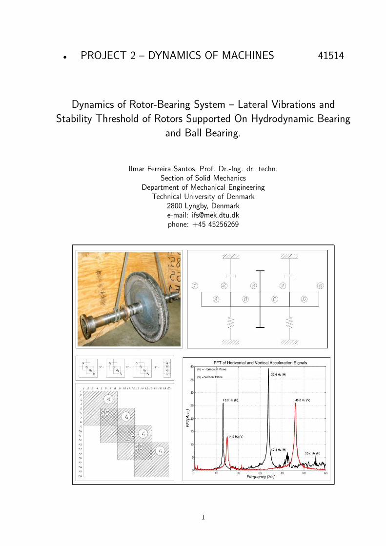
• PROJECT 2 – DYNAMICS OF MACHINES 41514
Dynamics of Rotor-Bearing System – Lateral Vibrations and
Stability Threshold of Rotors Supported On Hydrodynamic Bearing
and Ball Bearing.
Ilmar Ferreira Santos, Prof. Dr.-Ing. dr. techn.
Section of Solid Mechanics
Department of Mechanical Engineering
Technical University of Denmark
2800 Lyngby, Denmark
e-mail: [email protected]
phone: +45 45256269
1

1 Introduction
The occurrence of instability in rotating machines is a very typical problem in high speed machinesand may be caused by fluid-structure interactions due to oil film forces presented in hydrodynamicbearings or aerodynamic forces resulting from sealing, among others. A machine designer normallywants to know the range of angular velocity in which the machine will operate stable and withoutvibration problems, i.e. maximum angular velocity and distance from the unstable operational range.
The aim of this second project in the discipline is to make you familiar with the prediction of criticalspeeds in rotating machines, stability threshold and unbalance response and maximum vibrationamplitude while crossing critical speed ranges.
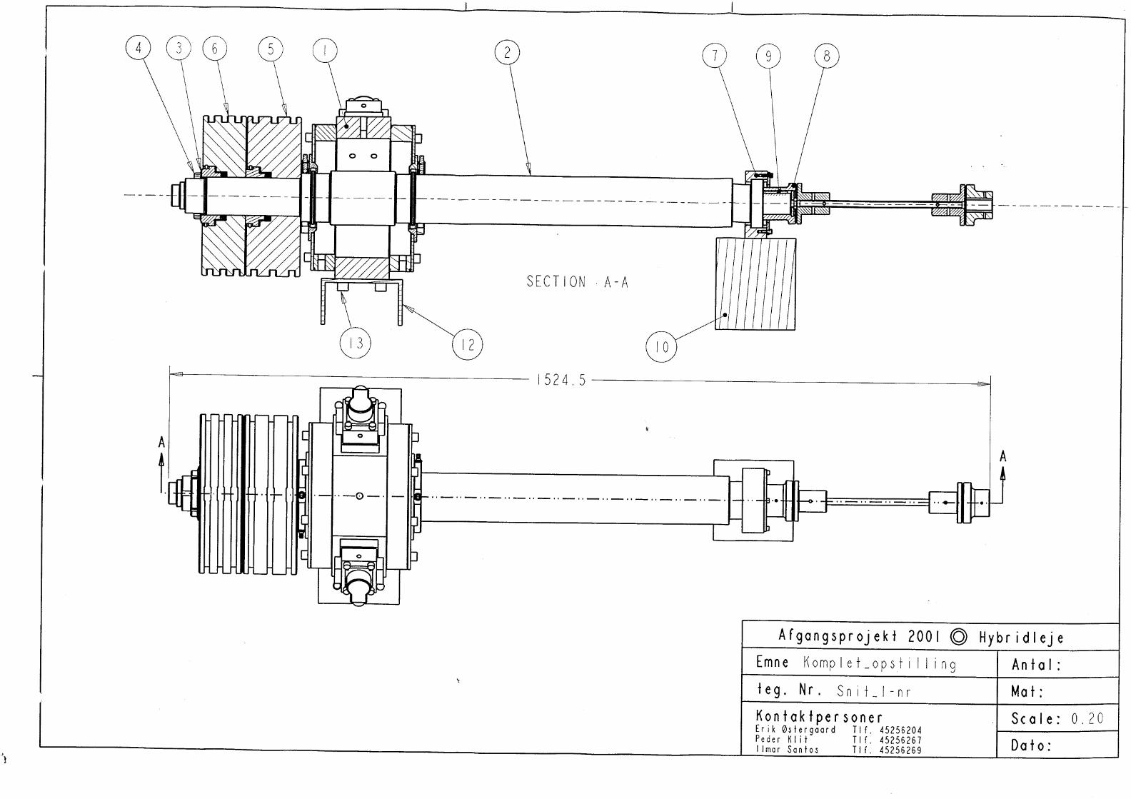
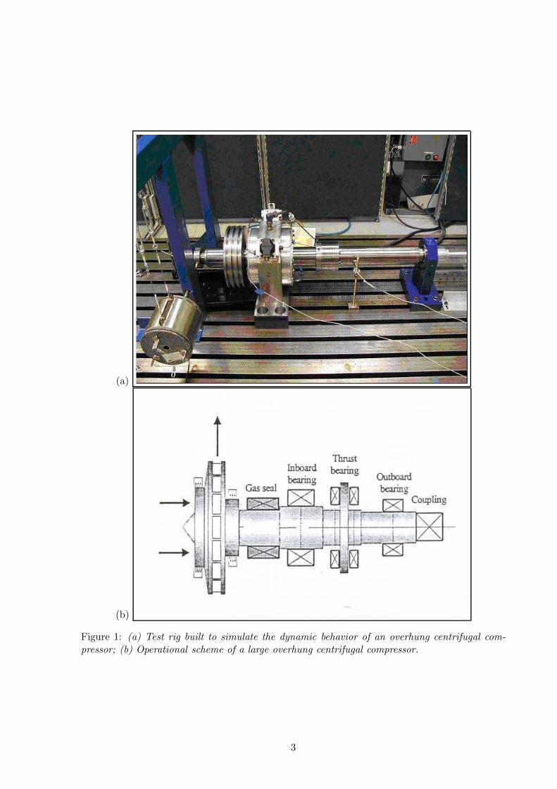
Aiming at dealing with a real rotor-bearing problem, the test rig illustrated in figure 1(a) will be usedas example of rotating machine. It will facilitate the visualization of the problem and aid the studentsto link the theoretical results to practical problems and experimental results. The test rig shown infigure 1(a) simulates a large overhung centrifugal compressor. The scheme of a large overhungcentrifugal compressor can be seen in figure 1(b). The test rig as well as the overhung centrifugalcompressor is composed of one flexible shaft, discs or impellers positioned at the end of the shaft.The shaft is laterally supported by two bearings. In the test rig the bearing closest to the coupling willoperate as thrust bearing as well. The sealing effect can be generated by an active magnetic bearingused as electromagnetic shaker without contact instead of active bearing, as illustrated in figure1(a). Nevertheless, the sealing effect will be disregarded in this educational project. All technicalinformation you need to carry out the project is put together in different drawings and in this projectdescription. By using all theoretical and experimental tools related to Rotor Dynamics obtainedduring the classes, you will hopefully win a very solid overview and understanding about how realand imaginary parts of eigenvalues – and consequently also eigenvectors – change as a function ofthe operational speeds.
The steps of the project are summarized following:
• Firstly you have to obtain mechanical and mathematical models of the flexible shaft element usingFinite Element Method (FEM). The first question you will face is the number of finite elements tobe used. Remember though that such models can be verified later using experimental modal analysiswhen the shaft is hanging in a free-free condition as you can see in figure 2(a). The model can beadjusted using the theoretical and experimental natural frequencies.
• Secondly the disc (impeller) shall be mounted onto the shaft. Mechanical and mathematicalmodels shall be expanded to cope with the dynamics of the disc. The model can be adjusted usingthe theoretical and experimental natural frequencies obtained from the experimental modal analysis,as it can be seen in figure figure 2(b) and figure 2(c).
• Finally, the flexible shaft connected to the rigid disc is mounted onto a ball bearing and a journalbearing, as it is shown in figure 1(a). The eigenvalues and eigenvectors will be calculated forthe global rotor-bearing-system. Damped natural frequencies (imaginary parts of the eigenvalues)will be obtained and their associated modes shapes will be visualized. Analyzing the real part of theeigenvalues insights into the stability of the rotor-bearing-system will be obtained. This will allow youto predict stable operational range. Two different types of hydrodynamic bearings will be simulatedduring the project in order to find out the bearing with the best dynamic properties, i.e. the bearingwhich provides the largest stable operational range.
2
(a)
(b)
Figure 1: (a) Test rig built to simulate the dynamic behavior of an overhung centrifugal com-pressor; (b) Operational scheme of a large overhung centrifugal compressor.
3
(a) (b)
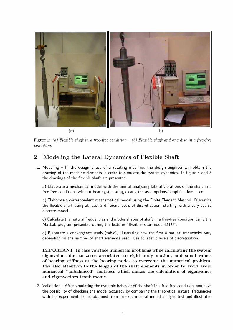
Figure 2: (a) Flexible shaft in a free-free condition – (b) Flexible shaft and one disc in a free-freecondition.
2 Modeling the Lateral Dynamics of Flexible Shaft
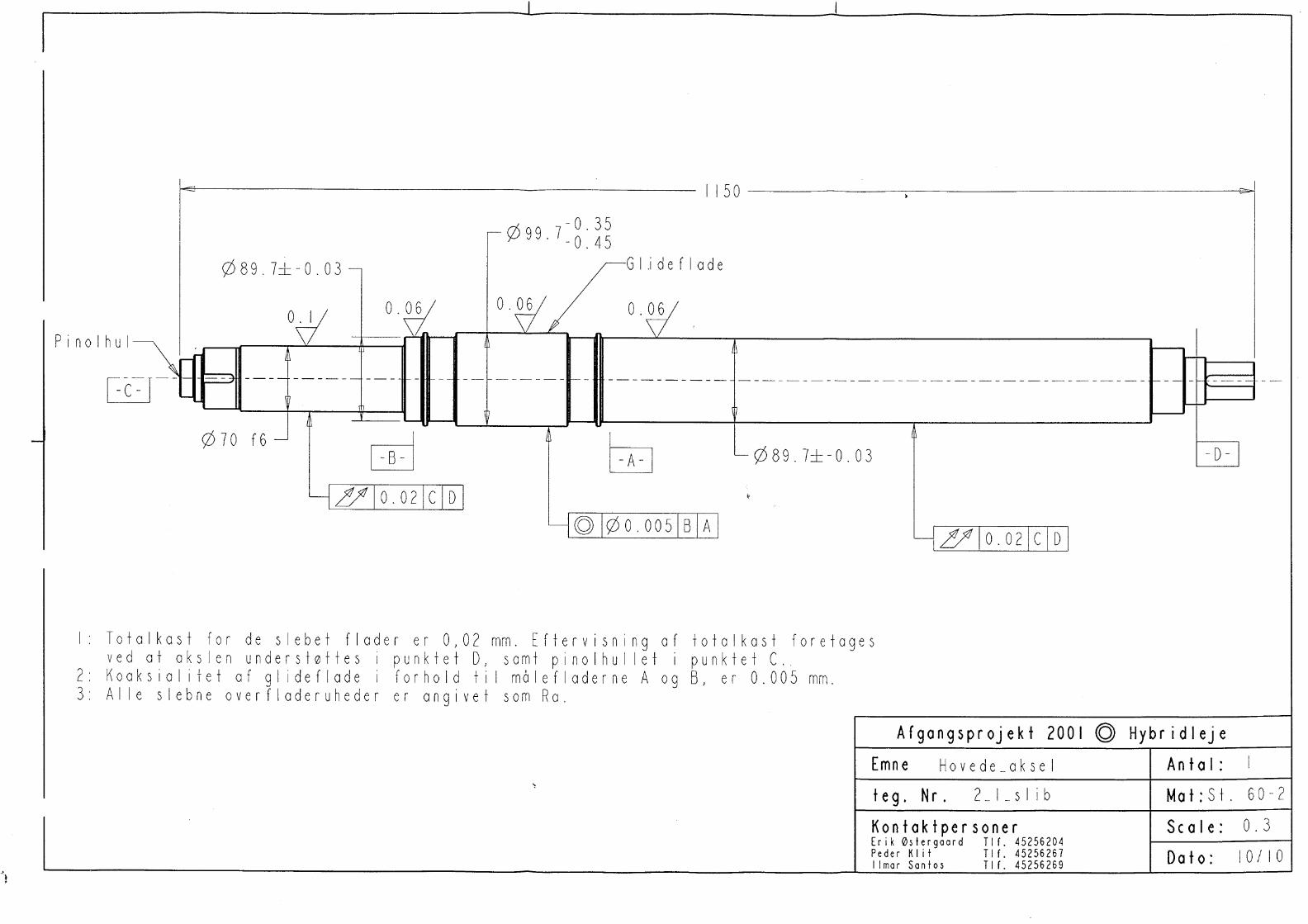
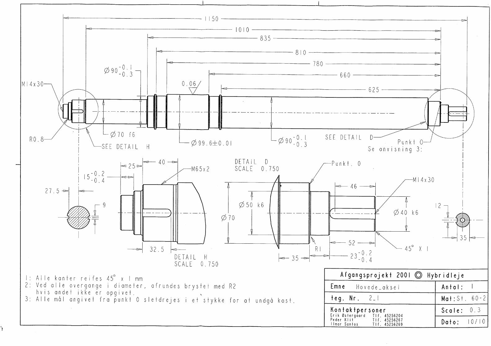
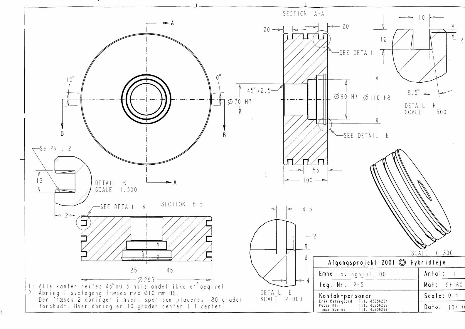
1. Modeling – In the design phase of a rotating machine, the design engineer will obtain thedrawing of the machine elements in order to simulate the system dynamics. In figure 4 and 5the drawings of the flexible shaft are presented.
a) Elaborate a mechanical model with the aim of analyzing lateral vibrations of the shaft in afree-free condition (without bearings), stating clearly the assumptions/simplifications used.
b) Elaborate a correspondent mathematical model using the Finite Element Method. Discretizethe flexible shaft using at least 3 different levels of discretization, starting with a very coarsediscrete model.
c) Calculate the natural frequencies and modes shapes of shaft in a free-free condition using theMatLab program presented during the lectures ”flexible-rotor-modal-DTU”.
d) Elaborate a convergence study (table), illustrating how the first 8 natural frequencies varydepending on the number of shaft elements used. Use at least 3 levels of discretization.
IMPORTANT: In case you face numerical problems while calculating the systemeigenvalues due to zeros associated to rigid body motion, add small valuesof bearing stiffness at the bearing nodes to overcome the numerical problem.Pay also attention to the length of the shaft elements in order to avoid avoidnumerical ”unbalanced” matrices which makes the calculation of eigenvaluesand eigenvectors troublesome.
2. Validation – After simulating the dynamic behavior of the shaft in a free-free condition, you havethe possibility of checking the model accuracy by comparing the theoretical natural frequencieswith the experimental ones obtained from an experimental modal analysis test and illustrated
4
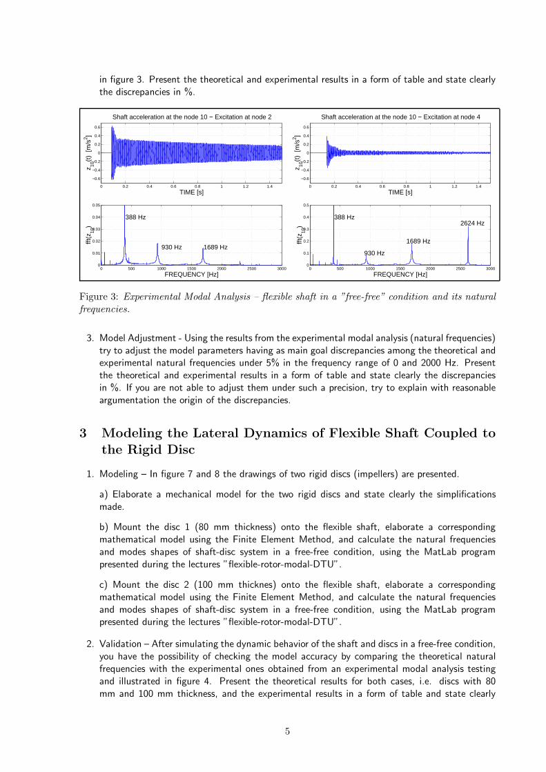
in figure 3. Present the theoretical and experimental results in a form of table and state clearlythe discrepancies in %.
0 0.2 0.4 0.6 0.8 1 1.2 1.4
−0.6
−0.4
−0.2
0
0.2
0.4
0.6
Shaft acceleration at the node 10 − Excitation at node 2
TIME [s]
z 10(t
) [m
/s2 ]
0 500 1000 1500 2000 2500 30000
0.01
0.02
0.03
0.04
0.05
FREQUENCY [Hz]
fft(z
10)
388 Hz
930 Hz 1689 Hz
0 0.2 0.4 0.6 0.8 1 1.2 1.4
−0.6
−0.4
−0.2
0
0.2
0.4
0.6
Shaft acceleration at the node 10 − Excitation at node 4
TIME [s]
z 10(t
) [m
/s2 ]
0 500 1000 1500 2000 2500 30000
0.1
0.2
0.3
0.4
0.5
FREQUENCY [Hz]
fft(z
10)
388 Hz
930 Hz
1689 Hz
2624 Hz
Figure 3: Experimental Modal Analysis – flexible shaft in a ”free-free” condition and its naturalfrequencies.
3. Model Adjustment - Using the results from the experimental modal analysis (natural frequencies)try to adjust the model parameters having as main goal discrepancies among the theoretical andexperimental natural frequencies under 5% in the frequency range of 0 and 2000 Hz. Presentthe theoretical and experimental results in a form of table and state clearly the discrepanciesin %. If you are not able to adjust them under such a precision, try to explain with reasonableargumentation the origin of the discrepancies.
3 Modeling the Lateral Dynamics of Flexible Shaft Coupled to
the Rigid Disc
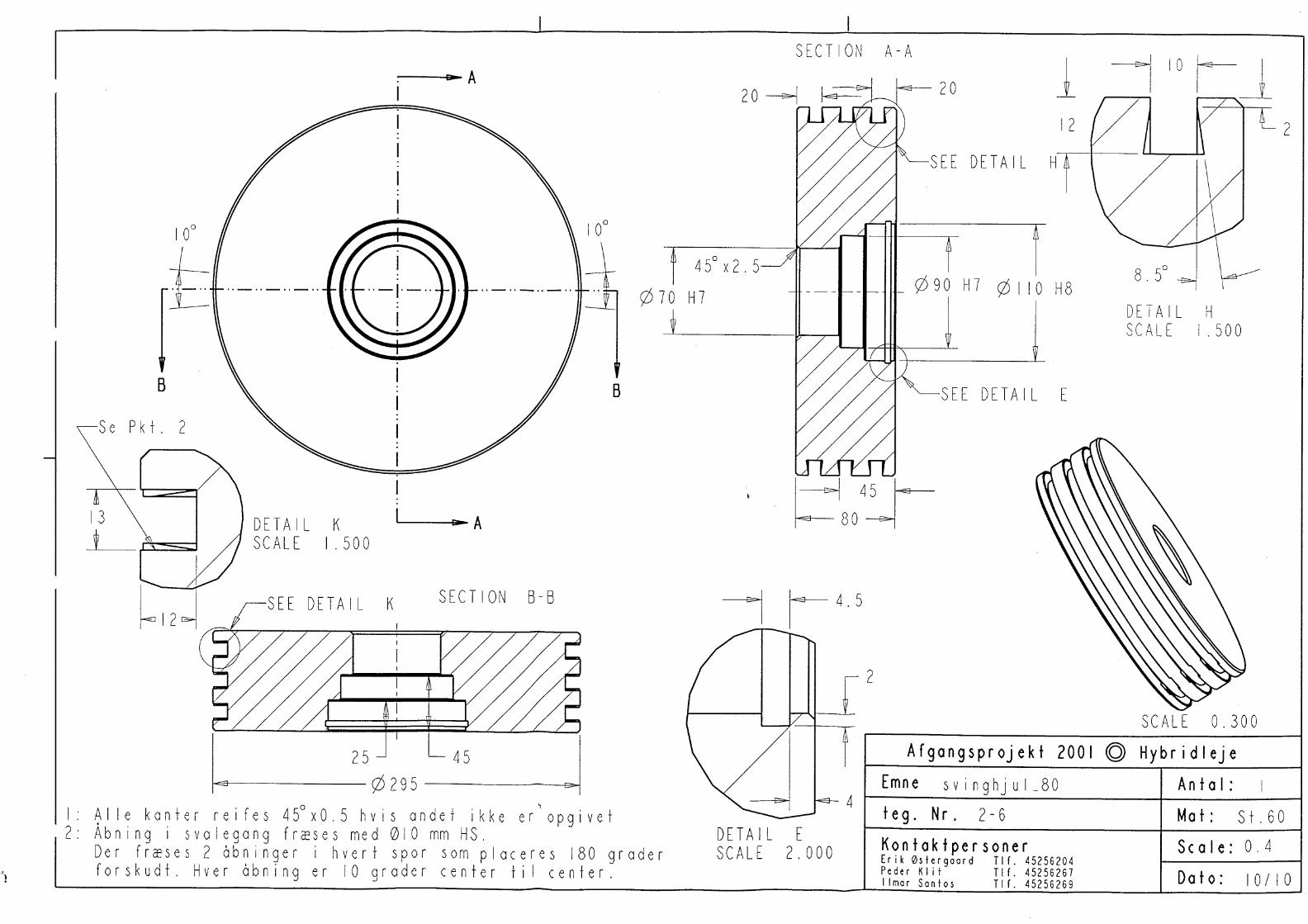
1. Modeling – In figure 7 and 8 the drawings of two rigid discs (impellers) are presented.
a) Elaborate a mechanical model for the two rigid discs and state clearly the simplificationsmade.
b) Mount the disc 1 (80 mm thickness) onto the flexible shaft, elaborate a correspondingmathematical model using the Finite Element Method, and calculate the natural frequenciesand modes shapes of shaft-disc system in a free-free condition, using the MatLab programpresented during the lectures ”flexible-rotor-modal-DTU”.
c) Mount the disc 2 (100 mm thicknes) onto the flexible shaft, elaborate a correspondingmathematical model using the Finite Element Method, and calculate the natural frequenciesand modes shapes of shaft-disc system in a free-free condition, using the MatLab programpresented during the lectures ”flexible-rotor-modal-DTU”.
2. Validation – After simulating the dynamic behavior of the shaft and discs in a free-free condition,you have the possibility of checking the model accuracy by comparing the theoretical naturalfrequencies with the experimental ones obtained from an experimental modal analysis testingand illustrated in figure 4. Present the theoretical results for both cases, i.e. discs with 80mm and 100 mm thickness, and the experimental results in a form of table and state clearly
5
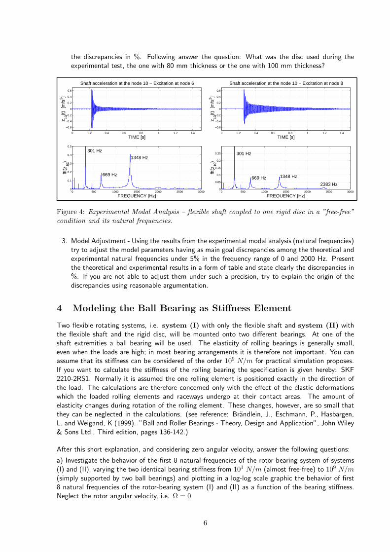
the discrepancies in %. Following answer the question: What was the disc used during theexperimental test, the one with 80 mm thickness or the one with 100 mm thickness?
0 0.2 0.4 0.6 0.8 1 1.2 1.4
−0.6
−0.4
−0.2
0
0.2
0.4
0.6
Shaft acceleration at the node 10 − Excitation at node 6
TIME [s]
z 10(t
) [m
/s2 ]
0 500 1000 1500 2000 2500 30000
0.1
0.2
0.3
0.4
0.5
FREQUENCY [Hz]
fft(z
10)
301 Hz
669 Hz
1348 Hz
0 0.2 0.4 0.6 0.8 1 1.2 1.4
−0.6
−0.4
−0.2
0
0.2
0.4
0.6
Shaft acceleration at the node 10 − Excitation at node 8
TIME [s]
z 10(t
) [m
/s2 ]
0 500 1000 1500 2000 2500 30000
0.05
0.1
0.15
0.2
0.25
FREQUENCY [Hz]
fft(z
10)
301 Hz
669 Hz 1348 Hz
2383 Hz
Figure 4: Experimental Modal Analysis – flexible shaft coupled to one rigid disc in a ”free-free”condition and its natural frequencies.
3. Model Adjustment - Using the results from the experimental modal analysis (natural frequencies)try to adjust the model parameters having as main goal discrepancies among the theoretical andexperimental natural frequencies under 5% in the frequency range of 0 and 2000 Hz. Presentthe theoretical and experimental results in a form of table and state clearly the discrepancies in%. If you are not able to adjust them under such a precision, try to explain the origin of thediscrepancies using reasonable argumentation.
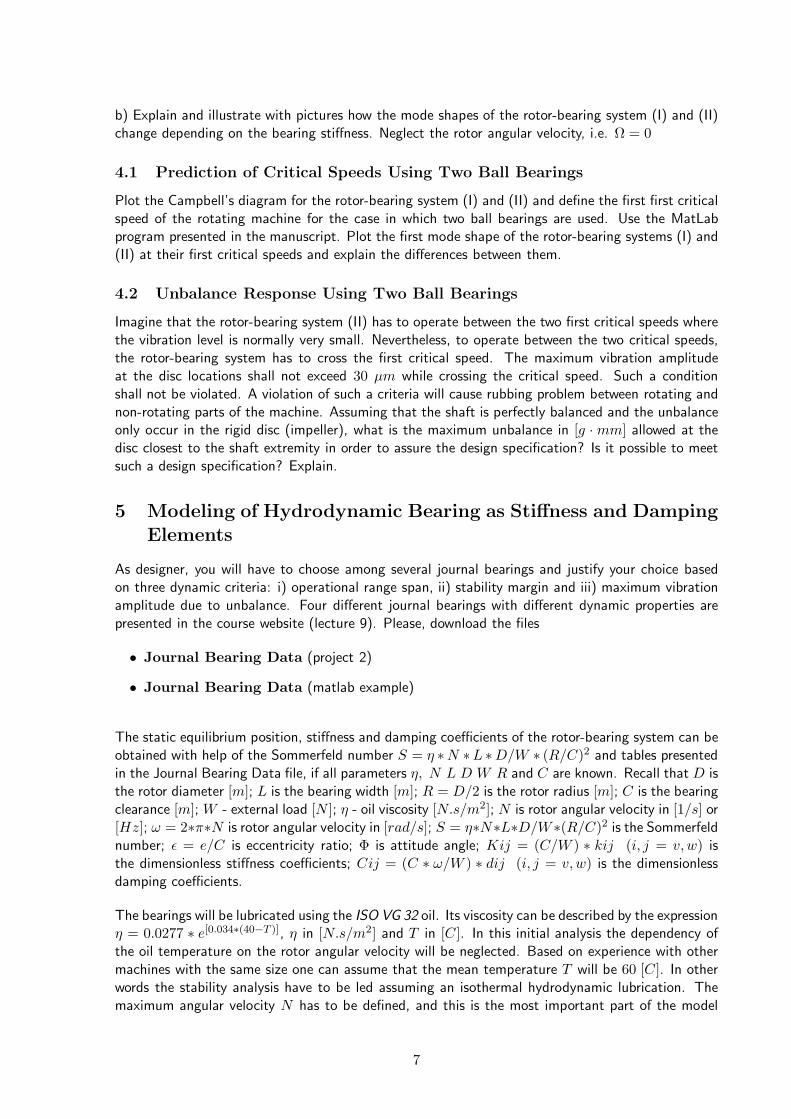
4 Modeling the Ball Bearing as Stiffness Element
Two flexible rotating systems, i.e. system (I) with only the flexible shaft and system (II) withthe flexible shaft and the rigid disc, will be mounted onto two different bearings. At one of theshaft extremities a ball bearing will be used. The elasticity of rolling bearings is generally small,even when the loads are high; in most bearing arrangements it is therefore not important. You canassume that its stiffness can be considered of the order 109 N/m for practical simulation proposes.If you want to calculate the stiffness of the rolling bearing the specification is given hereby: SKF2210-2RS1. Normally it is assumed the one rolling element is positioned exactly in the direction ofthe load. The calculations are therefore concerned only with the effect of the elastic deformationswhich the loaded rolling elements and raceways undergo at their contact areas. The amount ofelasticity changes during rotation of the rolling element. These changes, however, are so small thatthey can be neglected in the calculations. (see reference: Brandlein, J., Eschmann, P., Hasbargen,L. and Weigand, K (1999). ”Ball and Roller Bearings - Theory, Design and Application”, John Wiley& Sons Ltd., Third edition, pages 136-142.)
After this short explanation, and considering zero angular velocity, answer the following questions:
a) Investigate the behavior of the first 8 natural frequencies of the rotor-bearing system of systems(I) and (II), varying the two identical bearing stiffness from 101 N/m (almost free-free) to 109 N/m(simply supported by two ball bearings) and plotting in a log-log scale graphic the behavior of first8 natural frequencies of the rotor-bearing system (I) and (II) as a function of the bearing stiffness.Neglect the rotor angular velocity, i.e. Ω = 0
6
b) Explain and illustrate with pictures how the mode shapes of the rotor-bearing system (I) and (II)change depending on the bearing stiffness. Neglect the rotor angular velocity, i.e. Ω = 0
4.1 Prediction of Critical Speeds Using Two Ball Bearings
Plot the Campbell’s diagram for the rotor-bearing system (I) and (II) and define the first first criticalspeed of the rotating machine for the case in which two ball bearings are used. Use the MatLabprogram presented in the manuscript. Plot the first mode shape of the rotor-bearing systems (I) and(II) at their first critical speeds and explain the differences between them.
4.2 Unbalance Response Using Two Ball Bearings
Imagine that the rotor-bearing system (II) has to operate between the two first critical speeds wherethe vibration level is normally very small. Nevertheless, to operate between the two critical speeds,the rotor-bearing system has to cross the first critical speed. The maximum vibration amplitudeat the disc locations shall not exceed 30 µm while crossing the critical speed. Such a conditionshall not be violated. A violation of such a criteria will cause rubbing problem between rotating andnon-rotating parts of the machine. Assuming that the shaft is perfectly balanced and the unbalanceonly occur in the rigid disc (impeller), what is the maximum unbalance in [g · mm] allowed at thedisc closest to the shaft extremity in order to assure the design specification? Is it possible to meetsuch a design specification? Explain.
5 Modeling of Hydrodynamic Bearing as Stiffness and Damping
Elements
As designer, you will have to choose among several journal bearings and justify your choice basedon three dynamic criteria: i) operational range span, ii) stability margin and iii) maximum vibrationamplitude due to unbalance. Four different journal bearings with different dynamic properties arepresented in the course website (lecture 9). Please, download the files
• Journal Bearing Data (project 2)
• Journal Bearing Data (matlab example)
The static equilibrium position, stiffness and damping coefficients of the rotor-bearing system can beobtained with help of the Sommerfeld number S = η ∗N ∗L ∗D/W ∗ (R/C)2 and tables presentedin the Journal Bearing Data file, if all parameters η, N L D W R and C are known. Recall that D isthe rotor diameter [m]; L is the bearing width [m]; R = D/2 is the rotor radius [m]; C is the bearingclearance [m]; W - external load [N ]; η - oil viscosity [N.s/m2]; N is rotor angular velocity in [1/s] or[Hz]; ω = 2∗π∗N is rotor angular velocity in [rad/s]; S = η∗N∗L∗D/W∗(R/C)2 is the Sommerfeldnumber; ǫ = e/C is eccentricity ratio; Φ is attitude angle; Kij = (C/W ) ∗ kij (i, j = v,w) isthe dimensionless stiffness coefficients; Cij = (C ∗ ω/W ) ∗ dij (i, j = v,w) is the dimensionlessdamping coefficients.
The bearings will be lubricated using the ISO VG 32 oil. Its viscosity can be described by the expressionη = 0.0277 ∗ e[0.034∗(40−T )], η in [N.s/m2] and T in [C]. In this initial analysis the dependency ofthe oil temperature on the rotor angular velocity will be neglected. Based on experience with othermachines with the same size one can assume that the mean temperature T will be 60 [C]. In otherwords the stability analysis have to be led assuming an isothermal hydrodynamic lubrication. Themaximum angular velocity N has to be defined, and this is the most important part of the model
7
application. The rotor diameter D [m] can be obtained from the technical drawings. The relationshipR = D/2 and the bearing clearance C = 100 [µm] are pre-defined parameters. The relation L/Dwill be dependent on the bearing type used and is specified in the journal bearing data tables.
1. Before using/applying any kind of theoretical results, i.e. journal bearing data, a good engineerwill always try to clearly understand the theoretical assumptions/simplifications made in orderto obtain the theoretical results, in our case the tables. This engineering practice is very impor-tant and avoids engineers to use wrongly and inappropriately theoretical data, in ranges wherethe data should not be used. Violation of the theoretical assumptions leads consequently towrong analysis. In this framework, answer the following questions: what are the main assump-tions/simplifications made in order to obtain the Reynolds equation, foundation for building thejournal bearing data?
2. Calculate the external load due to the weight acting on the bearing W [N ]. For this purpose,please, use the geometry of the shaft elements and rigid discs elements . The Sommerfeldnumber will be a function of the angular speed of the machine N .
3. Using the journal bearing data tables illustrate graphically the behavior of the oil film thicknessin [µm] as function of the angular velocity N in [Hz] for the different types of journal bearings.Analyze the results.
4. a) Plot the values of stiffness coefficients [N/m] and damping coefficients [N/(m/s)] as afunction of the angular velocity N in [Hz] for the different types of journal bearings. Rememberthat the stiffness coefficients kij given in [N/m] are calculated as a function of kij = (W/C) ∗Kij (i, j = v,w), where Kij are the dimensionless stiffness coefficients obtained from thejournal bearing data tables. The damping coefficients dij given in [N/(m/s)] are calculated asa function of kij = W/(C ∗ ω) ∗ Cij (i, j = v,w), where Cij are the dimensionless dampingcoefficients obtained from the journal bearing data tables.
b) interpolate piecewise functions, for example splines or linear functions, to describe the be-havior of the stiffness and damping coefficients as a function of the angular velocity. Plot thestiffness and damping coefficients and the interpolated functions.
c) Write some conclusions about direct stiffness coefficients, cross coupling stiffness coefficientsand direct damping coefficients.
5.1 Prediction of Critical Speeds
1. Define the two first critical speeds of the rotor-journal bearing system (II) based on the Camp-bell’s diagram considering the four different hydrodynamic bearing types. Write the two firstcritical speeds for each of the four cases in a table, specifying bearing type, first critical speedand second critical speed.
2. Imagine that the rotor-bearing system has to operate between the two first critical speeds wherethe vibration level is normally very small. What is the bearing type which allows for the largestoperational velocity range?
5.2 Prediction of Rotor Bearing Stability Limit
1. Based on the stability maps of each of the four rotor-bearing systems (II), calculate the maximumangular speed N that the system can operate without instability problems resulting from theinteraction with the oil film forces? Write in a table, bearing type and maximum angular speed(instability threshold).
8
2. What is the best journal bearing from the viewpoint of stability threshold?
3. When the rotor-bearing system becomes unstable, the system vibration amplitude increases.What is the frequency of such an unstable vibration for the four different cases?
4. What is the relationship between the unstable frequency [Hz] and the rotor angular velocity Ω[Hz] in the stability threshold for the four different cases?
5.3 Unbalance Response
The maximum vibration amplitude at the disc locations shall not exceed 30 µm along the wholeoperational speed range. Such a condition shall not be violated. A violation of such a criteria willcause rubbing problem between rotating and non-rotating parts of the machine. Assuming that theshaft is perfectly balanced and the unbalance only occur in the rigid disc (impeller), what is themaximum unbalance in [g ·mm] allowed at the disc in order to assure the design specification.
1. Write in a table, bearing type and maximum unbalance in [g ·mm] allowed.
2. What is the best journal bearing from the viewpoint of unbalance response and maximumunbalance allowed?
5.4 Engineering Design – Application1
1. Bearing Design – The relationship R = D/2 and the bearing clearance C = 110 [µm] wereup to now pre-defined parameters and the relation L/D will be dependent on the bearing typeused and specified in the journal bearing data tables. As design engineer, chose one of thehydrodynamics bearings, and answer the following questions:
a) How variations in the bearing clearance C [µm] can influence the critical speeds?
b) How variations in the bearing clearance C [µm] can influence the limit of stability?
c) How variations in the bearing clearance C [µm] can influence the unbalance response?
2. Rotor Design – In the beginning of the project two rigid discs were presented with differentthickness, i.e. 80 mm and 100 mm. If you would use the other rigid disc with different mass andinertia properties, how the stability margin of the new rotor-bearing system would be affected?In other words, would the rotor-bearing system be able to be driven faster without instabilityproblems?
1For the students who want to fight for a 12 grade
9
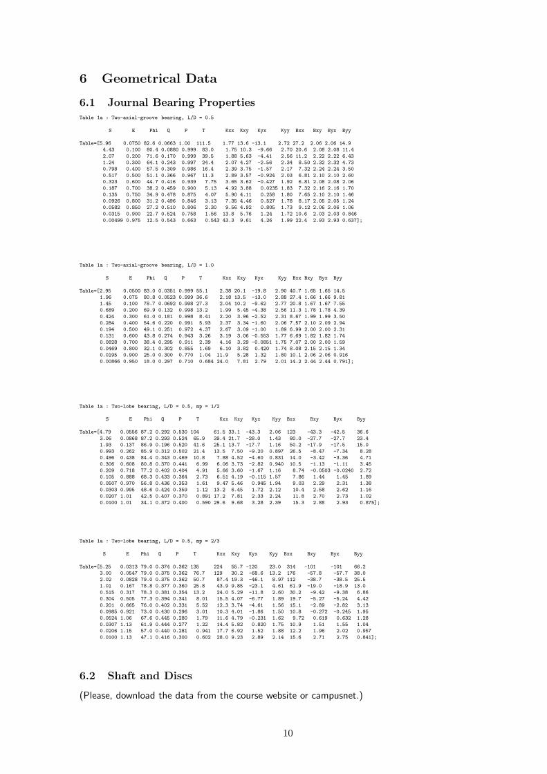
6 Geometrical Data
6.1 Journal Bearing Properties
Table 1a : Two-axial-groove bearing, L/D = 0.5
S E Phi Q P T Kxx Kxy Kyx Kyy Bxx Bxy Byx Byy
Table=[5.96 0.0750 82.6 0.0663 1.00 111.5 1.77 13.6 -13.1 2.72 27.2 2.06 2.06 14.9
4.43 0.100 80.4 0.0880 0.999 83.0 1.75 10.3 -9.66 2.70 20.6 2.08 2.08 11.4
2.07 0.200 71.6 0.170 0.999 39.5 1.88 5.63 -4.41 2.56 11.2 2.22 2.22 6.43
1.24 0.300 64.1 0.243 0.997 24.4 2.07 4.27 -2.56 2.34 8.50 2.32 2.32 4.73
0.798 0.400 57.5 0.309 0.986 16.4 2.39 3.75 -1.57 2.17 7.32 2.24 2.24 3.50
0.517 0.500 51.1 0.366 0.967 11.3 2.89 3.57 -0.924 2.03 6.81 2.10 2.10 2.60
0.323 0.600 44.7 0.416 0.939 7.75 3.65 3.62 -0.427 1.92 6.81 2.08 2.08 2.06
0.187 0.700 38.2 0.459 0.900 5.13 4.92 3.88 0.0235 1.83 7.32 2.16 2.16 1.70
0.135 0.750 34.9 0.478 0.875 4.07 5.90 4.11 0.258 1.80 7.65 2.10 2.10 1.46
0.0926 0.800 31.2 0.496 0.846 3.13 7.35 4.46 0.527 1.78 8.17 2.05 2.05 1.24
0.0582 0.850 27.2 0.510 0.806 2.30 9.56 4.92 0.805 1.73 9.12 2.06 2.06 1.06
0.0315 0.900 22.7 0.524 0.758 1.56 13.8 5.76 1.24 1.72 10.6 2.03 2.03 0.846
0.00499 0.975 12.5 0.543 0.663 0.543 43.3 9.61 4.26 1.99 22.4 2.93 2.93 0.637];
Table 1a : Two-axial-groove bearing, L/D = 1.0
S E Phi Q P T Kxx Kxy Kyx Kyy Bxx Bxy Byx Byy
Table=[2.95 0.0500 83.0 0.0351 0.999 55.1 2.38 20.1 -19.8 2.90 40.7 1.65 1.65 14.5
1.96 0.075 80.8 0.0523 0.999 36.6 2.18 13.5 -13.0 2.88 27.4 1.66 1.66 9.81
1.45 0.100 78.7 0.0692 0.998 27.3 2.04 10.2 -9.62 2.77 20.8 1.67 1.67 7.55
0.689 0.200 69.9 0.132 0.998 13.2 1.99 5.45 -4.38 2.56 11.3 1.78 1.78 4.39
0.424 0.300 61.0 0.181 0.998 8.41 2.20 3.96 -2.52 2.31 8.67 1.99 1.99 3.50
0.284 0.400 54.6 0.220 0.991 5.93 2.37 3.34 -1.60 2.06 7.57 2.10 2.09 2.94
0.194 0.500 49.1 0.251 0.972 4.37 2.67 3.09 -1.00 1.89 6.99 2.00 2.00 2.31
0.131 0.600 43.8 0.274 0.943 3.26 3.19 3.06 -0.553 1.77 6.69 1.82 1.82 1.74
0.0828 0.700 38.4 0.295 0.911 2.39 4.16 3.29 -0.0851 1.75 7.07 2.00 2.00 1.59
0.0469 0.800 32.1 0.302 0.855 1.69 6.10 3.82 0.420 1.74 8.08 2.15 2.15 1.34
0.0195 0.900 25.0 0.300 0.770 1.04 11.9 5.28 1.32 1.80 10.1 2.06 2.06 0.916
0.00866 0.950 18.0 0.297 0.710 0.684 24.0 7.81 2.79 2.01 14.2 2.44 2.44 0.791];
Table 1a : Two-lobe bearing, L/D = 0.5, mp = 1/2
S E Phi Q P T Kxx Kxy Kyx Kyy Bxx Bxy Byx Byy
Table=[4.79 0.0556 87.2 0.292 0.530 104 61.5 33.1 -43.3 2.06 123 -43.3 -42.5 36.6
3.06 0.0868 87.2 0.293 0.524 65.9 39.4 21.7 -28.0 1.43 80.0 -27.7 -27.7 23.4
1.93 0.137 86.9 0.196 0.520 41.6 25.1 13.7 -17.7 1.16 50.2 -17.9 -17.5 15.0
0.993 0.262 85.9 0.312 0.502 21.4 13.5 7.50 -9.20 0.897 26.5 -8.47 -7.34 8.28
0.496 0.438 84.4 0.343 0.469 10.8 7.88 4.52 -4.60 0.831 14.0 -3.42 -3.36 4.71
0.306 0.608 80.8 0.370 0.441 6.99 6.06 3.73 -2.82 0.940 10.5 -1.13 -1.11 3.45
0.209 0.718 77.2 0.402 0.404 4.91 5.66 3.60 -1.67 1.16 8.74 -0.0503 -0.0240 2.72
0.105 0.888 68.3 0.433 0.364 2.73 6.51 4.19 -0.115 1.57 7.86 1.44 1.45 1.89
0.0507 0.970 56.8 0.436 0.353 1.61 9.47 5.46 0.945 1.94 9.03 2.29 2.31 1.38
0.0303 0.995 48.6 0.424 0.359 1.12 13.2 6.45 1.72 2.12 10.4 2.58 2.62 1.16
0.0207 1.01 42.5 0.407 0.370 0.891 17.2 7.81 2.33 2.24 11.8 2.70 2.73 1.02
0.0100 1.01 34.1 0.372 0.400 0.590 29.6 9.68 3.28 2.39 15.3 2.88 2.93 0.875];
Table 1a : Two-lobe bearing, L/D = 0.5, mp = 2/3
S E Phi Q P T Kxx Kxy Kyx Kyy Bxx Bxy Byx Byy
Table=[5.25 0.0313 79.0 0.374 0.362 135 224 55.7 -120 23.0 314 -101 -101 66.2
3.00 0.0547 79.0 0.375 0.362 76.7 129 30.2 -68.6 13.2 176 -57.8 -57.7 38.0
2.02 0.0828 79.0 0.375 0.362 50.7 87.4 19.3 -46.1 8.97 112 -38.7 -38.5 25.5
1.01 0.167 78.8 0.377 0.360 25.8 43.9 9.85 -23.1 4.61 61.9 -19.0 -18.9 13.0
0.515 0.317 78.3 0.381 0.354 13.2 24.0 5.29 -11.8 2.60 30.2 -9.42 -9.38 6.86
0.304 0.505 77.3 0.394 0.341 8.01 15.5 4.07 -6.77 1.89 19.7 -5.27 -5.24 4.42
0.201 0.665 76.0 0.402 0.331 5.52 12.3 3.74 -4.61 1.56 15.1 -2.89 -2.82 3.13
0.0985 0.921 73.0 0.430 0.296 3.01 10.3 4.01 -1.86 1.50 10.8 -0.272 -0.245 1.95
0.0524 1.06 67.6 0.445 0.280 1.79 11.6 4.79 -0.231 1.62 9.72 0.619 0.632 1.28
0.0307 1.13 61.9 0.444 0.277 1.22 14.4 5.82 0.820 1.75 10.9 1.51 1.55 1.04
0.0206 1.15 57.0 0.440 0.281 0.941 17.7 6.92 1.52 1.88 12.2 1.96 2.02 0.957
0.0100 1.13 47.1 0.416 0.300 0.602 28.0 9.23 2.89 2.14 15.6 2.71 2.75 0.841];
6.2 Shaft and Discs
(Please, download the data from the course website or campusnet.)
10