PROJECT DURATION FORECASTING: A COMPARISON OF … · TABEL OF CONTENTS . ... EVA calculations (May...
101
PROJECT DURATION FORECASTING: A COMPARISON OF EARNED VALUE ANALYSIS METHOD TO EARNED SCEHEDULE AS OF TIME DURATION A Master Thesis Submitted to the Faculty of The WORCESTER POLYTECNIC INSTITUITE Civil and Environmental Engineering In partial fulfillment of the requirement for the DEGREE OF MASTER OF SCIENCE IN Interdisciplinary Construction Project Management By Mumtaz Abdullah Abdulahad April 30, 2015 Approved by Prof. Guillermo Salazar PhD, Major Advisor. ---------------------- Prof. Leonard Albano PhD, Thesis Committee ----------------------- Prof. Tahar El-Korchi PhD, Head of Department. ---------------------- 1
Transcript of PROJECT DURATION FORECASTING: A COMPARISON OF … · TABEL OF CONTENTS . ... EVA calculations (May...

PROJECT DURATION FORECASTING:
A COMPARISON OF EARNED VALUE ANALYSIS
METHOD TO EARNED SCEHEDULE AS OF TIME DURATION
A Master Thesis
Submitted to the Faculty of The
WORCESTER POLYTECNIC INSTITUITE
Civil and Environmental Engineering In partial fulfillment of the requirement for the
DEGREE OF MASTER OF SCIENCE
IN
Interdisciplinary Construction Project Management
By
Mumtaz Abdullah Abdulahad
April 30, 2015
Approved by
Prof. Guillermo Salazar PhD, Major Advisor. ----------------------
Prof. Leonard Albano PhD, Thesis Committee -----------------------
Prof. Tahar El-Korchi PhD, Head of Department. ----------------------
1

ABSTRACT
Earned Value Analysis (EVA) is a well- known planning and control management system that
integrates cost, schedule and technical performance. It allows for the calculation of cost and
schedule variances, performance indices as well as for the forecasting of project final cost and
schedule duration. The Earned Value Analysis method provides timely assessment of project
performance highlighting the need for eventual corrective action. EVA was originally
developed for cost management and has not been widely used for forecasting project duration.
EVA typically calculates the Schedule Efficiency through the Schedule Performance Index
(SPI) based on budgeted cost and not on the time of work accomplished. Therefore, it may not
accurately determine the time – base schedule efficiency, particularly for late completion
projects, and it makes it difficult to correlate the final duration with project planned duration
determined through Critical Path Method (CPM) network calculations. Earned Schedule (ES)
is a method based on EVA but it develops a set of time dependent schedule indicators which
perform consistently over the entire period of project performance and improve the accuracy
of forecasting the duration of the project and its completion date.
The purpose of this study is to compare the classic EVA performance indicators with the time
dependent ES performance indicators in order to help project managers to estimate and/or
predict a more realistic and reliable time duration of project that can better correlate with
CPM. It also explores how Building Information Modeling (BIM) simulation tools could be
incorporated into EVA to visually communicate and quantify the timely phased physical
progress during the development of project as opposed to the traditional use of cash flow
analysis.
2

ACKNOWLEDGMENTS
The author would like to express his thanks and gratitude to his advisor Dr. Guillermo Salazar
for his useful comments, remarks and engagement through the learning process of this Master
Thesis. Furthermore, I would like to thank Dr. Tahar El- Korchi Head of Civil &
Environmental Department at WPI who has willingly supported me.
I would like to thank Prof. Leonard Albano, a thesis committee member for his precious time
and for providing valuable insight during the review process.
At the end, I would like to thank and express appreciation to my loved wife Ban Atto and my
children Maryam & Abdullah for their support and keeping me harmonious in the moments
when there was no one to answer my queries.
Special thanks and respect to my deceased parents who had put me on the path.
Mumtaz A. Abdulahad
3

TABEL OF CONTENTS
Contents
Chapter 1 Introduction ................................................................................................. 8 Objectives of this Study ......................................................................................................................................... 9
Chapter 2. Earned Value Analysis ............................................................................... 11 2.1 Earned Value Analysis Parameters ......................................................................................................... 12 2.2 Establishing Performance Management Baseline (PMB) .............................................................. 14
2.2.1 Performance Management Baseline Characteristics ..................................................................... 15 2.2.2 Performance Management Baseline Data Relationships ............................................................. 16 2.2.3 Control Accounts Plan (CAP) ..................................................................................................................... 18
2.3 Objectives of creating an Organization Breakdown Structure .................................................... 19 2.4 Critical Path Method (CPM) ........................................................................................................................ 20 2.5 Measuring Options of Earned Value Analysis ..................................................................................... 23 2.6 Project Status Indicators (Metrics), ........................................................................................................ 26
2.6.1 PP – Percentage Planned. ........................................................................................................................... 26 2.6.2 PA – Percentage Actual. ............................................................................................................................ 27 2.6.3 PC – Percentage Complete ........................................................................................................................ 27 2.6.4 To Complete Cost Performance Indicator (TCPI) .......................................................................... 29 2.6.5 Schedule Variance (SV) ................................................................................................................................ 29 2.6.6 Schedule Performance Indicator (SPI). ................................................................................................ 30 2.6.7 To Complete Schedule Performance Index (Indicator) (TSPI) .................................................. 31 2.6.8 Estimate To Complete (ETC) ..................................................................................................................... 32 2.6.9 Estimate At Completion (EAC) ................................................................................................................. 32
2.7 Variance At Completion (VAC). ................................................................................................................. 37 2.8 Implementation Requirements for EVA ................................................................................................ 43 2.9 Project Control ................................................................................................................................................. 45
2.9.1 Scaling EVA to fit varying situations ..................................................................................................... 46 2.10 Benefits of Earned Value Analysis (EVA) ........................................................................................... 47
2.10.1 Limitations of Earned Value Analysis (EVA) ................................................................................... 49
Chapter 3. Earned Schedule ........................................................................................ 50 3.1 Earned Schedule Concepts and Calculations ....................................................................................... 51 3.2 Earned Schedule Measures and Indicators .......................................................................................... 55
Example 1 ...................................................................................................................................................................... 60 Example 2 ...................................................................................................................................................................... 61 Example 3 ..................................................................................................................................................................... 66
Chapter 4 CASE STUDY ................................................................................................ 72 4.1 Earned Value Analysis, Earned Schedule and Building Information Modeling (BIM) ....... 72
4
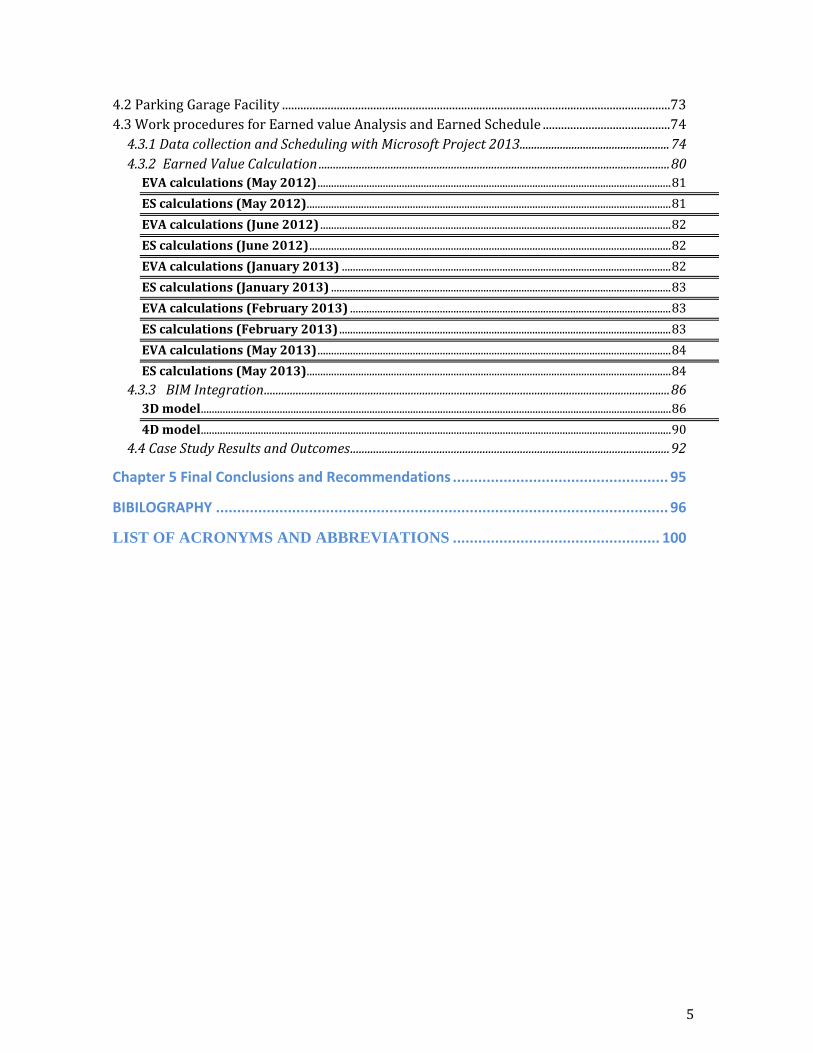
4.2 Parking Garage Facility ................................................................................................................................ 73 4.3 Work procedures for Earned value Analysis and Earned Schedule .......................................... 74
4.3.1 Data collection and Scheduling with Microsoft Project 2013 .................................................... 74 4.3.2 Earned Value Calculation .......................................................................................................................... 80
EVA calculations (May 2012) .................................................................................................................................. 81 ES calculations (May 2012) ...................................................................................................................................... 81 EVA calculations (June 2012) ................................................................................................................................. 82 ES calculations (June 2012) ..................................................................................................................................... 82 EVA calculations (January 2013) ......................................................................................................................... 82 ES calculations (January 2013) ............................................................................................................................. 83 EVA calculations (February 2013) ...................................................................................................................... 83 ES calculations (February 2013) .......................................................................................................................... 83 EVA calculations (May 2013) .................................................................................................................................. 84 ES calculations (May 2013) ...................................................................................................................................... 84
4.3.3 BIM Integration ............................................................................................................................................. 86 3D model ............................................................................................................................................................................. 86 4D model ............................................................................................................................................................................. 90
4.4 Case Study Results and Outcomes ............................................................................................................... 92
Chapter 5 Final Conclusions and Recommendations ................................................... 95
BIBILOGRAPHY ........................................................................................................... 96
LIST OF ACRONYMS AND ABBREVIATIONS ................................................. 100
5
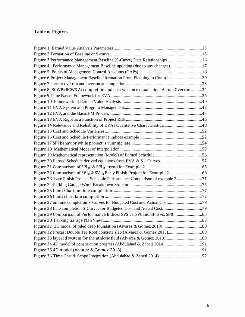
Table of Figures Figure 1 Earned Value Analysis Parameters ................................................................................................. 13 Figure 2 Formation of Baseline or S-curve. ................................................................................................... 15 Figure 3 Performance Management Baseline (S-Curve) Data Relationships ...................................... 16 Figure 4 Performance Management Baseline updating (due to any changes) ................................... 17 Figure 5 Points of Management Control Accounts (CAPs) ..................................................................... 18 Figure 6 Project Management Baseline formation From Planning to Control .................................... 20 Figure 7 current overrun and overrun at completion ................................................................................... 33 Figure 8 BCWP=BCWS At completion and cost variance equals final Actual Overrun. ........... 34 Figure 9 Time Basics Framework for EVA .................................................................................................... 36 Figure 10 Framework of Earned Value Analysis ........................................................................................ 40 Figure 11 EVA System and Program Management ..................................................................................... 42 Figure 12 EVA and the Basic PM Process ..................................................................................................... 45 Figure 13 EVA Rigor as a Function of Project Risk ................................................................................... 46 Figure 14 Relevance and Reliability of EVAs Qualitative Characteristics. ......................................... 48 Figure 15 Cost and Schedule Variances .......................................................................................................... 52 Figure 16 Cost and Schedule Performance indices example .................................................................... 52 Figure 17 SPI behavior while project is running late .............................................................................. 54 Figure 18 Mathematical Model of Interpolation .......................................................................................... 55 Figure 19 Mathematical representation (Model) of Earned Schedule ................................................... 56 Figure 20 Earned Schedule derived equations from EVA & S – Curves. ............................................ 57 Figure 21 Comparison of SPI (t) & SPI ($) trend for Example 2 .............................................................. 65 Figure 22 Comparison of SV (t) & SV ($) Early Finish Project for Example 2 .................................... 66 Figure 23 Late Finish Project, Schedule Performance Comparison of example 3 ........................... 71 Figure 24 Parking Garage Work Breakdown Structure .............................................................................. 75 Figure 25 Gantt Chart on time completion .................................................................................................. 77 Figure 26 Gantt chart late completion .......................................................................................................... 77 Figure 27 on time completion S-Curves for Budgeted Cost and Actual Cost ..................................... 78 Figure 28 Late completion S-Curves for Budgeted Cost and Actual Cost. .......................................... 79 Figure 29 Comparison of Performance Indices SV$ vs. SVt and SPI$ vs. SPIt ............................... 85 Figure 30 Parking Garage Plan View ............................................................................................................ 87 Figure 31 3D model of piled deep foundation (Alvarez & Gomez 2013) ........................................... 88 Figure 32 Precast Double Tee Roof concrete slab (Alvarez & Gomez 2013) ..................................... 89 Figure 33 layered system for the athletic field (Alvarez & Gomez 2013) ........................................ 89 Figure 34 4D model of construction progress (Abdulahad & Zabeti 2014) ......................................... 91 Figure 35 4D model (Alvarez & Gomez 2013) ........................................................................................ 91 Figure 36 Time Cost & Scope Integration (Abdulahad & Zabeti 2014) ............................................... 92
6

List of Tables
Table 1 EV Measurement Techniques ............................................................................................................ 26 Table 2 Prediction Table for meeting the budget and planned time. ..................................................... 31 Table 3 Earned Value Analysis Terms. ........................................................................................................... 38 Table 4 Earned Value Analysis Formulas ....................................................................................................... 39 Table 5 Interpretation of Basic EVA Performance Measures ................................................................... 41 Table 6 Summary of EVA and ES Performance Metrics ........................................................................... 59 Table 7 Early Finish Project Example 2 ........................................................................................................... 65 Table 8 Late Finish Project Example 3 ............................................................................................................ 70 Table 9 Parking Garage Data for EVA & ES Analysis ............................................................................. 76 Table 10 Comparison between EVA final duration forecast vs. ES final duration forecast. .......... 84
List of Equations
Equation 1 ................................................................................................................................................................. 13 Equation 2 ................................................................................................................................................................. 13 Equation 3 ................................................................................................................................................................. 21 Equation 4 ................................................................................................................................................................. 22 Equation 5 ................................................................................................................................................................. 22 Equation 6 ................................................................................................................................................................. 23 Equation 7 ................................................................................................................................................................. 27 Equation 8 ................................................................................................................................................................. 28 Equation 9 ................................................................................................................................................................. 28 Equation 10 .............................................................................................................................................................. 30 Equation 11 .............................................................................................................................................................. 56 Equation 12 .............................................................................................................................................................. 57
7

Chapter 1 Introduction
Earned Value Analysis (EVA) was taken from industrial engineering in factories where
planned standards and earned standard were linked primarily to labor hours (Lanner
2004). In the mid 1960’s,the United States Air force started setting standards to oversee
Department of Defense (DoD) contractors performance. The resulting system was DoD
Cost / Schedule Control System Criteria C/SCSC issued in 1991 revision which included
35 detailed criteria for performance reporting that were later reduced to 32 (Abba 1995),
Abba 1999 ).
EVA has shown to be a reliable tool for monitoring project progress when sufficient
information regarding the project work to be done can be linked to specific scope
deliverables and to the organization’s resources needed to perform the work (Lanner
PMP 2004). EVA also provides reliable performance measurement of time progress as
early as the 15% percent completion point of a project (Fleming and Koppelman 2002).
However its ability to predict schedule delays has come into question as it does not take
into account the time value of money (Fleming & Koppelman 2003 & 1994 C), which
makes project managers less confident and depend on their intuitions to assess the final
completion time of late completion projects.
The Earned Schedule (ES) is an extension of the EVA method. It is an emerging practice
in project management (Lipke 2003), (Lipke 2012). It determines the time at which the
Earned Value accrued should have been occurred according to the original plan and
calculates the time variance in terms of time and not in terms of cost. It also focus
8

significantly on monitoring and forecasting project schedule performance using the
standard Earned Value Analysis (EVA) technique, i.e., performance indicators, Budgeted
Cost of Work Scheduled ((BCWS), Budgeted Cost of Work Performed (BCWP), Actual
Cost of Work Performed (ACWP), and Budget at Completion (BAC). This concept
improves time metrics accuracy in latter periods of project performance and overcomes
the major limitation of EVA for late completion projects by providing meaningful time
metrics for the entire period of project performance.
Building Information Modeling (BIM) is an enabling technology that promotes
collaboration among parties and allows to visualize in 3D different design options
helping clients and designers to better understand different options. It can be used to
check cost estimates by quantifying the material from 3D model and helping to detect the
clashes of different building components. It can also be used to track the project
milestones in phases to foresee the progress of project throughout construction. A 5D
model combines the 3D view of the model plus its time and cost implications and
explicitly displays dynamic correlation among the three variables scope – time and cost
in clear visual fashion facilitating the understanding of the impact that each variable has
on the other two as well as on the communication among the project participants.
Objectives of this Study
It is the purpose of this study to:
• Compare EV performance Indicators with time dependent ES Indicators to
determine a more realistic time duration that can be correlated with CPM.
9

• Demonstrate that by using the ES concept, the project managers do not need to
depend only upon their intuition to forecast the final duration of “late completion
projects” when they can rely on a robust method for determining the entire time
duration or earned schedule of project tasks that better correlate with CPM and
stakeholders expectations.
• Explore how Building Information Modeling (BIM) simulation tools could be
incorporated into EVA to visually communicate and quantify the timely phased
physical progress during the development of project as opposed to the traditional
use of cash flow analysis.
The above objectives are attained by conducting a exhaustive review of Earned Value
Analysis (EVA), and Earned Schedule (ES) concepts and procedures and by developing a
Case Study based on the design and construction of the recently built WPI Parking
Garage with Rooftop Athletic fields. This case study compares the results generated by
the use of EVA and ES and explores the use of BIM in conjunction with ES through the
creation of 4D and 5D simulations.
10

Chapter 2. Earned Value Analysis
This study involves the utilization of Earned Value Analysis concept (EVA), which is a
performance management tool that integrates cost, schedule and technical performance to
facilitate graphic presentation of Schedule and Cost Performance compared to plan. (Lipke
2003), (Wilkens 1993). Before going deeply in the subject, the following definitions and
meanings existing in Earned Value Analysis (EVA) terminology are introduced:
1. Earned Value Analysis (EVA): is a quantitative project management technique for
evaluating project performance and predicting final project results, based on comparing
the progress and budget of work packages to planned work and actual costs.
2. Earned Value Management (EVM): is a project management methodology for controlling
a project which relies on measuring the performance of work using a Work Breakdown
Structure (WBS) and includes an integrated schedule and budget based on the project
WBS.
3. Earned Value Management System (EVMS): is the process, procedures, tools and
templates used by an organization to conduct Earned Value Management (Lukas 2008).
The Earned Value Analysis (EVA) was developed as a tool to facilitate project control. It is
used for determining a project’s status with regards to cost and schedule. It uses cost variance
and schedule variance to determine the amount of deviations from the plan as early as
possible, so that enough time is made available for project managers to assess whether the
deviation may have potential negative impact, and to take corrective actions. Moreover, it
allows project managers to make inferences on the final effect of the project in terms of cost
11

to and some extent, in terms of duration, by extrapolating from current trends (Brake 2006),
(Czarnigowska 2008), (Rose 2011).
2.1 Earned Value Analysis Parameters Earned Value Analysis parameters are used to track the progress of projects and to compare
deviations (if any) against the planned performance also known as Budgeted Costs of Works
Scheduled (BCWS) that both the contracted parties (owner and the contractor) have agreed
upon in the contract. These parameters require definition of the following inputs or elements
as follow:
At = Actual Time of work in progress at the reporting date.
PD = Planned Duration of the project Baseline (days, weeks, months, years).
t = Reporting Date
T’= Actual Completion Date.
Figure (1) below shows the general representation of how Earned Value Analysis (EVA)
parameters cover the whole aspects of project performance and how they contribute to set
mathematical relationship for each metric. This happens for any project regardless of its size
and cost.
12

Figure 1 Earned Value Analysis Parameters
As one can see, the Earned Value Analysis concept mainly consists of three curves: Budgeted
Costs of Works Scheduled (BCWS), which is the baseline for the analysis is a function that
links cumulated planned costs with time of their time occurrence (PMBOK, 2008), (PMBOK
2013). It represents the sum of budgets for all work packages scheduled to be accomplished
within a given time. This is calculated as
BCWS = Hourly Rate* total hours planned for any given time (t)
Or, the cumulative summation of the cost of all time-related work packages. As shown in
Equation (2) below
Equation 2
Equation 1
13

This curve (BCWS) is also known as Performance Management Baseline (PMB), which will
be thoroughly explained in the following pages due to its significant value in determining the
feasibility degree of Earned Value Analysis metrics in the management of projects. Budgeted
Cost of Work Scheduled (BCWS) is sometimes defined as Planned Value (PV) curve, or
sometimes called the “Baseline” or S-curve only. So,
BCWS = PV = PMB = S- curve
2.2 Establishing Performance Management Baseline (PMB)
The Work Breakdown Structure (WBS) is a deliverable-oriented grouping of project elements
(granularity) that organize and defines the total scope of the project. Each descending
hierarchical structure represents an increasing detailed definition of project work.
Figure (2) below displays the process of establishing PMB based on the WBS. It includes
three main elements: definition of work, schedule the work, and allocation of budget which
are derived from the Work Breakdown Structure (WBS). Therefore, costs, schedule and
responsibilities are consistently associated to each of the tasks. For a large project, it will be a
tedious task to calculate these elements manually, therefore one can rely on scheduling
software like Microsoft Project, Primavera P6 that could be used to calculate and associate
these three elements.
14

Figure 2 Formation of Baseline or S-curve.
Source: http://www.humphreys-assoc.com/evms/basic-concepts-earned-value-management-evm-ta-a-74.html
2.2.1 Performance Management Baseline Characteristics
The Performance Management Baseline has the following characteristics (EVMIG 2006):
1. It accurately represents only authorized work on the contract.
2. It includes a realistic network schedule baseline.
3. It includes a realistic time phased spread of budget/resources to the baseline schedule.
It is worth to mention that besides the above mentioned points, Building Information
Modeling (BIM) tools can be used effectively in the creation of Performance Management
Baseline due to the accurate quantification of project elements as well as other time saving
functionalities such as clash detection, and coordinating ability for updating of last minute
negotiation changes. These are significant factors which have contributed to make the Earned
Value Analysis concept more rigorous and vital in controlling the project performance.
15

2.2.2 Performance Management Baseline Data Relationships
Figure (3) below shows the relationship between the “Work Breakdown Structure” (WBS
representing the scope of work) and a time-phased schedule of work to be done with realistic
cost estimates for each of the “Work Packages” in the project.
Figure 3 Performance Management Baseline (S-Curve) Data Relationships
Source: http://www.leaderelper.com/pdf-files/LCSI-EV6111-4-Hour-EarnedValue-KeySlides.pdf
As changes to the WBS, cost estimate and/or schedules are approved, the Baseline should
be updated as shown in Figure (4), and performance is compared to the new Baseline.
16
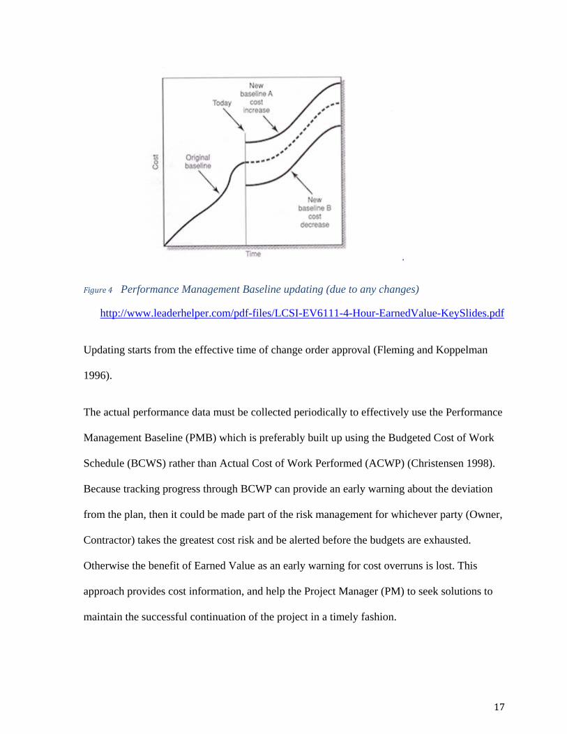
Figure 4 Performance Management Baseline updating (due to any changes)
http://www.leaderhelper.com/pdf-files/LCSI-EV6111-4-Hour-EarnedValue-KeySlides.pdf
Updating starts from the effective time of change order approval (Fleming and Koppelman
1996).
The actual performance data must be collected periodically to effectively use the Performance
Management Baseline (PMB) which is preferably built up using the Budgeted Cost of Work
Schedule (BCWS) rather than Actual Cost of Work Performed (ACWP) (Christensen 1998).
Because tracking progress through BCWP can provide an early warning about the deviation
from the plan, then it could be made part of the risk management for whichever party (Owner,
Contractor) takes the greatest cost risk and be alerted before the budgets are exhausted.
Otherwise the benefit of Earned Value as an early warning for cost overruns is lost. This
approach provides cost information, and help the Project Manager (PM) to seek solutions to
maintain the successful continuation of the project in a timely fashion.
17

2.2.3 Control Accounts Plan (CAP) Figure (5) below, shows a Management Control Diagram, known as the Control Accounts
Plan (CAPs), where the management control is maintained through the (CAP). CAPs are used
to measure the Earned Value at the most basic level of formation.
(
Figure 5 Points of Management Control Accounts (CAPs)
Source: www.humphreys-assoc.com) basic concepts of Earned Value Analysis
The elements that are necessary to create a Control Accounts Plan (CAPs) include :
1- Establishing the Scope of work (WBS).
The Work Breakdown Structure (WBS) is a deliverable-oriented grouping of project
elements that organizes and defines the total scope of the project. Each hierarchical
structure represents an increasingly detailed definition of the project work.
2- Creating a Schedule of Activities.
18

By using an updated project management software planner such as Microsoft Project
it is possible to create sequential series of interrelated activities.
3- Establishing a Budgeted Cost of activities.
This could be done with the help of previous historical documents of similar activities
that the firm has accomplished.
4- Assigning a Team Leader to manage the planning and lifecycle of project.
This could be done through a Responsibility Assignment Matrix (RAM) which
depicts the relationship between Work Breakdown Structure (WBS) elements and
Organization Breakdown Structure (OBS) elements that assigned responsibility for
ensuring accomplishment of the project work.
5- Creating large homogenous WBS levels.
6- Determine multiple functions integrated with WBS.
2.3 Objectives of creating an Organization Breakdown Structure An Organizational Breakdown Structure (OBS) is created in order to establish a clear picture
of the total project work scope, and to assign responsibilities to the right people. The
organizational process includes the following:
1. Create a WBS by decomposing the work into manageable work packages.
2. Define the Organization Breakdown Structure.
3. Assign a single work package to single party in the Organizational Breakdown
Structure.
4. Create Control Account Plans (CAPs) as indicated, implies to create the controlling
aspects for interrelated Schedule and Budget. (Humphreys 2001).
19

Figure (6) below shows how “Work Packages” with their associated detailed information for
planning and tracking are consolidated by period to create an S- Curve / Baseline Schedule
against which the amount of Budgeted Cost of Work Performed (BCWP) is expected to be
completed each planning period.
Figure 6 Project Management Baseline formation From Planning to Control
Source: http://www.humphrevs-assoc.com/evms/basic-concepts-earned-value-management-evm-ta-a74.html
2.4 Critical Path Method (CPM) The Critical Path Method is a network analysis technique used to predict project duration by
analyzing which sequence of activities (which path) has the least amount of scheduling
flexibility the least amount of Total Float or the amount of time that a task in a project
network can be delayed without causing a delay to subsequent tasks thus delaying project
completion date. The Critical Path is also defined as the largest path duration of interrelated
20
sequenced activities on project network of a program which is the BCWS Planned Duration
(PD) itself also.
Total Float can be measured by subtracting the early dates from late dates of path completion.
T.F = L F of current task – E F of current task
The Free Float (F.F) is the amount of time that an activity can be delayed without delaying the
early start of its successor activity.
F.F = ES next task – EF current task
The following are some of the essential EVA parameters:
Budget At Completion (BAC) is the total planned cumulative cost of all work packages in
the project, it equals BCWS at Planned Duration (PD). It could also be defined as a
cumulative summation of a specific dollar of work scope (tasks) of a BCWS when all work
packages have been phased, the cumulative BCWS = BAC. It could also be the “Total
Budget” allocated to the project, plotted over time, say like periods of reporting (weekly,
monthly, yearly…etc.). BAC is used to compute the following EVA metrics:
• “Estimate At Completion” (EAC)
• To complete the Cost Index (TCPI)
• To Complete The Schedule Index (TSPI).
BAC is calculated using the following formulas:
BAC = (BCWS Efforts-hrs.)* (hourly Rate)
Equation 3
21

It is also calculated as the Cumulative Summation of all Time-phased Budgets of work
packages / BCWS, where work packages incorporate direct cost of construction material, and
equipment only.
Equation 4
In addition to Budgeted Cost of Work Schedule (BCWS), there is generally an amount of
Management Reserve (MR), which is a portion of the total program budget not allocated to
specific work packages and withheld for management control process. Thus, Budget At
Completion (BAC) consists of the BCWS plus all the Management Reserve (MR) amount.
Budgeted Cost of Work Performed (BCWP) or Earned Value (EV) (PMBOK 2008). It is a
measure of physical progress of work expressed by cumulated planned cost of work actually
done related to the date of reporting. It is also the total cost of work completed/performed as
of reporting date. It can also be seen as the sum of completed work packages and completed
portions of open work packages. Essentially it is the value of work earned.
This is calculated as:
BCWP = Budget At completion * % Complete
Equation 5
Where % Completed or PC = (Budgeted units) - (Units to complete) / Budgeted units.
It is worth to mention that on early completion or on time completion (on budget) the
Budgeted cost of work performed (BCWP) = (BCWS) = BAC.
22

Actual Cost of Work Performed (ACWP) or Actual Cost (AC), (PMBOK 2008) is the
cumulative actual cost of the work completed as of reported date. It is also the amount of
money (cost) or resources expended in order to accomplish the amount of work achieved for
the reporting period.
ACWP = (Hourly Rate) * (Total hours spent)
Equation 6
ACWP is the cumulative summation of actual cost spent for material, equipment and labor for
accomplished work over time.
2.5 Measuring Options of Earned Value Analysis Each control account manifests at a work package level the overall project plan for activities
to produce project deliverables (i.e., the schedule), the use of resources (i.e., the resource and
procurement plans), and the commitment and expenditure of funds (i.e., the cost budget).
Physical progress against each of these plan elements is measured to support Earned Value
Analysis and forecasting.
Some options might be adopted are: (Lanners 2004)
1. Milestones with weighted values. (These can be complex to set up). The weighted
milestone technique divides the work to be completed into segments, each ending with
an observable milestone; it then assigns a value to the achievement of each milestone.
The weighted milestone technique is more suitable for longer duration tasks having
intermediate, tangible outcomes. (limits over-estimating)
2. Fixed Formula (25/75; 50/50; 75/25), A typical example of fixed formula is the 50/50
technique. With this method, 50% of the work is credited as complete for the
23
measurement period in which the work begins, regardless of how much work has
actually been accomplished. The remaining 50% is credited when the work is
completed. Other variations of the fixed formula method include 25/75 and 0/100.
Fixed formula techniques are most effectively used on small, short-duration tasks.
3. Percent-Complete Estimate: the percent complete technique is among the simplest and
easiest, but can be the most subjective of the Earned Value measurement techniques if
there are no objective indicators to back it up. This is the case when, at each
measurement period, the responsible worker or manager makes an estimate of the
percentage of the work complete. These estimates are usually for the cumulative
progress made against the plan for each task. However, if there are objective indicators
that can be used to arrive at the percent complete (for example, number of units of
product completed divided by the total number of units to be completed), then this can
be a more useful technique. (Commonly used)
4. Percent-complete with Milestones Gate: this method is satisfactory if based on
objective metrics.
5. Equivalent Units: One man-hour works for eight hours is equivalent to eight men
working for one hour. Or converting the units of measurement used to quantify
different elements of work package into one “equivalent” unit. For example Tons of
Steel.
6. Earned Standards or Units Complete: It is good for longer work packages are being
done.
7. Apportioned Relationship to Discrete Work. (i.e., “burden”) for work that is not easily
measured like “soft” costs, but which is proportional to a measurable effort. Avoid
24

using an apportioned measure for a large value work package where the basis for the
apportioning is a significantly smaller value work package.
8. Level of Efforts (LOE). Work of general or supportive nature (such as coordination,
follow up, liaison) that doesn’t result in a definitive end product or outcome. It is not
recommended, as it does not measure the task schedule performance (SV), is based on
setting the Budgeted Cost of Work Performed (BCWP) equal to the Budgeted Cost of
Work Schedule (BCWS) for each performance reporting period. Thus, the schedule
performance (SV) is always zero. It does, however, provide early cost variance (CV)
visibility to a potential overrun on the (LOE) tasks. Level of Efforts (LOE) is
applicable for management, measuring Earned Value for the Management Reserve
(MR), and administrative tasks as being unmeasurable tasks. Accordingly, some
authors advise not to use it as much as possible as it distort the overall project’s earned
value as portion of the Earned Value derived from (LOE) work packages grow relative
to the total project planned value.
Recommended usage of options:
a. Options from No. 1 to No. 4 are typically used for non-recurring tasks.
b. Options from No. 5 to No. 6 are used for either non-recurring or recurring tasks.
c. Option No. 7 could be used for any points from 1 to 6.
d. Option No. 8 is not recommended for use.
The guidelines for selecting of BCWP Measurement Techniques are outlined in the
following Table (1) below.
25

Product of Work Duration of Work Effort
1-3 Measurement Periods > 3 Measurement Periods
Tangible Fixed formula Weighted Milestone, Percent
Complete
Intangible Apportioned Effort, Level of effort.
Table 1 EV Measurement Techniques
2.6 Project Status Indicators (Metrics), Earned Value Analysis has large number of metrics used to track and monitor the progress of
work in the project, the most important and basic metrics are listed as follows:
2.6.1 PP – Percentage Planned. It is the percentage of work which was planned to be completed by the reporting date. This is
calculated using the following formula:
PP = BCWS/BAC*100
The range of this metric for 0 ~ 100%
26

2.6.2 PA – Percentage Actual. It is the percentage of work was actually completed by the reporting date, sometimes defined
as Percent Spent. This is calculated using the following formula:
PA = ACWP/BAC x 100
The range of this metric is from 0 ~ ∞. (due to cost overrun in late completion project).
2.6.3 PC – Percentage Complete It is the percent of work earned by the work completed as of reporting date.
This is calculated using the following formula
PC = BCWP/BAC x 100
The range of this metric is from 0 ~ 100%.
Cost Variance (CV) is a very important factor (Metric) to measure project performance. Cost
Variance indicates how much over or under budget the project is by the reporting date. Cost
Variance represents the gap between Budgeted Cost of Work Performed (BCWP) versus
Actual Cost incurred (ACWP) as of reported date.
Cost Variance can be calculated using the following formula,
CV = BCWP – ACWP
Equation 7
The formula above gives the variance in terms of cost which indicates how less or how much
more has been used to complete the work as of date.
• Positive Cost Variance indicates the project is under the budget.
• Negative Cost Variance indicates the project is over budget.
27

Cost Variance Percentage (CV%) it is an indicator of cost that shows how much over or
under budget the project is in terms of percentage. Cost Variance Percentage can be calculated
using the following formula:
CV % = (BCWP – ACWP) / BCWP (as of reporting date) x 100
Equation 8
The above equation determines the variance (gap) in terms of percentage which will indicate
how much less or how much more money has been used to complete the work as planned in
terms of percentage.
• Positive variance %, Indicates %, under budget,
• Negative %, Indicates % over budget.
Cost Performance Indicator (CPI). It is an Index value showing the efficiency of utilizing
the “resources” on the project. Cost Performance Index (metric) can be calculated using the
following formula:
CPI = BCWP/ACWP
Equation 9
It measures the efficiency of the project team in utilizing the resources allocated to the
project team, and can be used to predict the final range of costs.
• CPI value above (1) indicates efficiency in utilizing the resources allocated to the
project.
28

• CPI value below (1) indicates deficiency in utilizing the resources allocated to the
project. So, CPI is a metric of a project team efficiency in utilizing the resource
allocated for the project as of reported date.
2.6.4 To Complete Cost Performance Indicator (TCPI) To Complete Performance Index (Indicator): It is a forecasting indicator or metric
showing the efficiency at which the resources on the project should be used for the
remainder of the work to meet the planned Budget At Completion (BAC). Or is a portion
between the remaining work and the money left from the Budget. (Czarnigowska 2008).
This metric can be calculated using the following formula.
TPCI = (BAC – BCWP) / (BAC- ACWP)
• TCPI value above (1) indicates utilizing of the project team resources for the
remainder of the project can be stringent.
• TCPI value less under (1) indicates utilization of the project team resources for the
remainder of the project can be lenient.
2.6.5 Schedule Variance (SV) Schedule Variance indicates how much time in terms of cost/ volume of the work (i.e. $ 1.0 =
one unit volume of work) is the project ahead or behind schedule. It shows the gap between
the work performed versus the planned work. Schedule variance can be calculated as using the
following formula.
Schedule Variance (SV) = BCWP - BCWS
Schedule Variance Percentage (SV%). Indicates how much time ahead or behind schedule
the project is in terms of percentage of time. It can be calculated using the following formula
29

SV% = Schedule variance (SV) *100
BCWS as of reported date
Equation 10
So, it is an indicator (metric) of time consumed for the accomplished work.
The aforesaid formula gives the variance in terms of monetary value as percentage, which will
indicate how much percentage of work (cost) is yet to be completed as per the schedule or
how much percentage of work has been completed over and above the scheduled cost.
• Positive variance %, indicates % ahead of schedule
• Negative variance %, indicates % behind the schedule
2.6.6 Schedule Performance Indicator (SPI). Schedule Performance Indicator (SPI). It is an Index showing the efficiency of the "time"
utilized on the project. Schedule Performance Indicator can be calculated using the following
formula,
SPI = BCWP / BCWS
The formula above shows efficiency of the project team in utilizing the time allocated for the
project. And can be used to assess how much work has been accomplished to date?
• SPI value above (1) indicates the project team is efficiently in utilizing the time
allocated to the project.
• SPI value below (1) indicates the project team is not efficient in utilizing the time
allocated to the project.
• SPI ratio equal (1) indicates the project team efficiency of time is as planned.
30

2.6.7 To Complete Schedule Performance Index (Indicator) (TSPI) To Complete Schedule Performance Index, is a forecasting metric showing the efficiency at
which the remaining time on the project should be utilized. This can be calculated using the
following formula
TSPI = [BAC - BCWP] / [BAC - BCWS]
The formula mentioned above gives the efficiency at which the resources should be utilized
the "remaining time" allocated for the project.
• TSPI value below (1) indicates project team can be lenient in utilizing the remaining
time allocated to the project.
• TSPI value above (1) indicates project team needs to work harder in utilizing the
remaining time allocated to the project.
The following prediction table (2) provides information concerning whether to attempt
corrective action or negotiate a change with the customer.
TSPI Predicted action
Less or equal 1 Achievable
More than 1.1 Non-achievable
Table 2 Prediction Table for meeting the budget and planned time.
31

2.6.8 Estimate To Complete (ETC) Estimate To Complete (ETC), is the estimated cost/funds required to complete the remainder
of the project (work) at any point in time. This indicator is calculated and applied when the
past estimating assumption due to program halt became invalid and a need for fresh estimates
arise. Estimate To Complete (ETC) is used to complete the Estimate At Completion (EAC).
ETC is determined using the following formula:
ETC= BAC – ACWP
Where, ACWP is the actual cost to date and BAC is the budget at completion.
ETC is also the difference between estimate at completion (EAC) and Actual Cost of Work
Performed (ACWP). This is the estimated additional cost/funds required to complete the
remaining work on the task (s) from any given time.
2.6.9 Estimate At Completion (EAC) Estimate At Completion (EAC), is a forecast defining the most likely total estimated cost &
time based on project performance and risk quantification. At the start of the project, BAC
and EAC will be equal. EAC will vary from BAC only when the ACWP vary from the BCWS
(Nagrecha 2002). Moreover, it is observed that one of the more beneficial aspects of Earned
Value concept is its ability to provide an independent forecast for the total funds required at
the end of the project (Fleming & Koppelman 1994C).
EAC is the cost allocated to the work to date plus the Estimated Cost to Complete for
authorized work remaining (Nguyen 1993). It is observed that the Estimate At Completion
(EAC), is an important number and is very controversial, largely because there is literally an
infinite number of possible EAC formulas (Christensen 1998). During a project, the cost
control process focuses on cost overruns, of which there are two kinds:
32

1. Current Cost Overrun being presently experience (as of date), i.e., cost variance.
2. Forecasted Cost Overrun at completion, based on EAC.
These two kinds are shown in Fig (7) below
Figure 7 current overrun and overrun at completion
Therefore at any point of time in the project’s development, there is always a need to forecast
cost at completion. This information is often requested from project managers by anxious
senior management and is vital to the project cash flow, the viability of project, and
sometimes whether to cancel the project after it has started (Harrison 1981). It is worth noting
that at the end of the project, BCWP equals BCWS and cost variance equals the final actual
overrun, provided the scope does not change (see Figure 8 below)
33
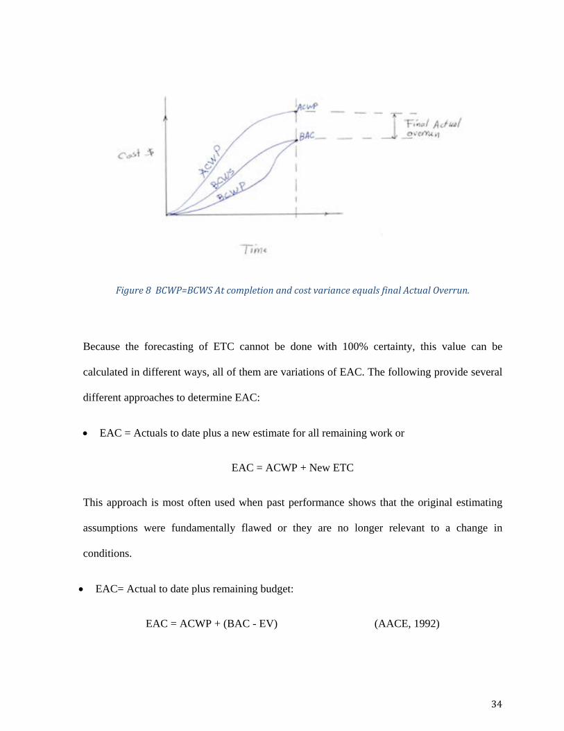
Figure 8 BCWP=BCWS At completion and cost variance equals final Actual Overrun.
Because the forecasting of ETC cannot be done with 100% certainty, this value can be
calculated in different ways, all of them are variations of EAC. The following provide several
different approaches to determine EAC:
• EAC = Actuals to date plus a new estimate for all remaining work or
EAC = ACWP + New ETC
This approach is most often used when past performance shows that the original estimating
assumptions were fundamentally flawed or they are no longer relevant to a change in
conditions.
• EAC= Actual to date plus remaining budget:
EAC = ACWP + (BAC - EV) (AACE, 1992)
34

This approach is most often used when current variance are seen as "Typical" and the project
management team expectations are that similar variances will "not" occur in future.
• EAC = Actuals to date plus the remaining budget modified by a performance factor (PF)
often the Cumulative Cost Performance Index (CPI). This approach is most often used
when current variances are seen as "typical" of future variances (Turner 1993), (Fleming &
Koppelman 1996).
EAC = ACWP + (BAC- BCWP) / CPI cum. to date
• EAC = Budget At Completion (BAC) modified by a performance factor, cumulative Cost
Performance Index (CPI) (AACE 1992)
EAC = BAC / CPI cum to date.
This approach is often used when no variance from BAC has occurred or when future cost
performance will be the same as all past cost performance (measure of lower bound).
• When future cost performance will be the same as the last three measurement periods (i j
k), EAC can be calculated as follow:
EAC = ACWP+ [ (BAC- BCWP) / [(BCWPi +BCWPj + BCWPk) / (ACWPi+ ACWPj+ ACWPk)]
• When future cost performance will be influenced additionally by past schedule
performance, EAC can be calculated as follow:
EAC = ACWP + [ ( BAC – BCWP ) / ( CPI * SPI)] measure of upper bound
35

• When future cost performance will be influenced jointly in same proportion by both
indices. The following formula is most suitable (PMI - Practice Standard for Earned Value
Management).
EAC = ACWP+ [(BAC- BCWP) / (0.8 CPI + 0.2 SPI)]
The other EACt is the Estimated Finish Time or sometimes called “Actual Completion” as
shown in fig (9) where the suffix (t) represents the time duration expected to complete the
project. This Indicator is calculated by the following formula,
EACt = BAC / SPI / BAC / PD = PD / SPI
Where PD is the planned duration of the project.
Figure 9 Time Basics Framework for EVA
36

However this method generates a fairly rough estimate and must always be compared with the
statistics reflected by the time based schedule method such as Critical Path Method (CPM).
(Fleming and Koppelman, 2009).
2.7 Variance At Completion (VAC). This is another important metric in Earned Value Analysis Control System, which is defined
as the difference between what the total job is supposed to cost,i.e., BAC, and what the total
job is now expected to cost. This matric is calculated using the following formula (Refer to
Figure 1).
VAC = BAC - EAC
The importance of this metric as a Control System for contractor(s) and owner(s) can be better
understood by looking at how the positive or negative consequences on VAC impact each
party as follows.
Variation at completion (VAC) vs. Contractor loss on fixed price lump sum contract.
If VAC is positive:
EAC < BAC
If VAC is Negative:
EAC > BAC
Some practical recommendation for the owner can be derived from the calculation of EAC
metric.
Under run budget Contractor gain
Share area Contractor Partial loss
Over run Contractor loss 100% EAC> Ceiling
37

a) The owner should develop top level EAC for comparison
b) The owner will limit progress payment if EAC is greater than ceiling price.
c) The owner needs forecast of fund requirement. (Christensen, 1993).
Actual performance at 15% complete point can be used to predict final performance (Fleming
and Koppelman 1999). Thus when the EAC and VAC results are substantially different from
contractor's estimate BAC more than likely the project manager (PM) may question the
discrepancy.
The Project Manager (PM) can also use the Independent Estimate At Completion IEAC or
Estimate At Completion EAC to justify continuation of the project for upper management by
the EAC & VAC for reaching implications (Lipke, 2012). Table 3 below provides a summary
of Earned Value Analysis Terms
Table 3 Earned Value Analysis Terms.
Term Variable(Metric) Description
PV (BCWS) Planned Value What is the estimated value of the
work planned to be done.
EV (BCWP) Earned Value What is the estimated value of the work actually accomplished?
AC (ACWP) Actual Cost What is the actual cost incurred?
BAC Budget at Completion
How much did you BUDGET for the TOTAL JOB?
EAC
Estimate at Completion
What do we currently expect the TOTAL project to cost?
ETC Estimate to Complete
From this point on, how much MORE do we expect it to cost to finish the job?
VAC
Variance at Completion
How much over or under budget do we expect to be?
38

Table 4 summarizes Earned Value Analysis Formulas and their interpretation
Name Formula Interpretation
Cost Variance (CV) EV – AC NEGATIVE is over budget, POSITIVE is under budget.
Schedule Variance (SV) EV – PV NEGATIVE is behind
schedule, POSITIVE is ahead of schedule
Cost Performance Index (CPI) EV/AC I am {only} getting ____ cents
out of every $1.
Schedule Performance Index (SPI) EV/PV
I am {only} progressing at ____% of the rate originally
planned.
Estimate At Completion (EAC)
Note: There are many ways to calculate EAC
BAC/ CPI
AC+ETC
AC+BAC=EV
(BAC-EV)/CPI
As of now how much do we expect the total project to cost
$_____. Used if no variance from the BAC have occurred and
give lower boundary. Actual plus a new estimate
for remaining work. Used when original estimate was
fundamentally flawed. Actual to date plus
remaining budget. Used when current variances are atypical.
Actual to date plus remaining budget modified by
performance. when current variances are typical
Estimate To Complete (ETC) EAC- AC How much more will the
project cost?
Variance At Completion (VAC) BAC - EAC
How much over budget will we be at the end of the
project?
Table 4 Earned Value Analysis Formulas
39

After exploring and discussing the Earned Value Analysis terms and metrics, Figure (10)
shows how the EVA metrics relationships are set to form a framework.
Figure 10 Framework of Earned Value Analysis
40

Table (5) shows “at-a-glance” what EVA performance measures indicate about a project in
regard to its planned work schedule and resource budget.
Performance measures SV & SPI
> 0 & >1.0 (=)o & (=)1.0 < 0 & < 1.0
CV & CPI
> 0 & >1.0
Ahead of schedule ; under budget
On schedule ; under budget
Behind schedule; under budget
(=)o & (=)1.0
Ahead of schedule ; on budget
On schedule ; on budget
Behind schedule ; on budget
< 0 & < 1.0
Ahead of schedule ; over budget
On schedule; over budget
Behind schedule; over budget
Table 5 Interpretation of Basic EVA Performance Measures
SPACE LEFT BLANK INTENTIONALLY
41

Figure (11) below shows the relation between program management elements and general
program components
Figure 11 EVA System and Program Management
Proj
ect M
anag
emen
t Cyc
le
Initiate
Plan
Control
Close Out
Execute
Program manager needs
Organize the work and the team
Develop a realistic plan of the work scope, the budget and the schedule
Control Changes
Performance reporting
Understand variances
Authorize work properly
Corrective actions
Forecast of final cost & schedule
42
2.8 Implementation Requirements for EVA The following are requirements established by Fleming & Koppelman, for the
implementation of Earned Value Analysis in all projects (Fleming & Koppelman, 1996):
• Define work scope
You must define 100% of the work scope using a Work Breakdown Structure (WBS).
If you do not define 100% the constituents of the project, how can you measure the project
performance in definite way?
• Create an Integrated Bottom up Plan
By combining the critical process including defined work scope, schedule and estimated
resources into an integrated bottom up of detailed measurement cells called "control account
plans" [CAPs]
• Formally Schedule Control Account Plan (CAPs)
Each of the defined CAPs must be planned and scheduled with a formal scheduling system.
• Assign each CAP to an organizational unit for performance
Each of the defined CAPs must be assigned to a permanent functional responsible for
performance. This assignment effectively commits the executive to oversee the performance
of each CAP.
• Establish a Baseline that summarize CAPs
43

A total project performance measurement baseline must be established which represents the
summation of the detailed CAPs. Baseline must include all defined CAPs plus any
management (Contingency) reserve that may be held by the project manager.
If the management reserves (MR) are not given to the project manager but are instead
controlled by a senior management committee they should be excluded from the Project
Performance Baseline.
• Measurement Performance against Schedule
Periodically, the projects schedule performance against the planned master project schedule
must be measured.
The difference between the work accomplished and work planned constitute the (SV) in terms of Earned Value.
• Measure cost efficiency against cost incurred
Periodically, measure the project cost performance efficiency rate which represents the
relationship between the project's BCWP performed against Cost incurred (ACWP) to achieve
the Earned Value (EV).
• Forecast final cost based on performance
Periodically, forecast the project’s final cost requirements (EAC) based on its performance against plan.
• Managing Remaining Works
Continuously manage the project’s remaining works.
• Manage BCWS Changes
Continuously, maintain the project’s BCWS by managing all changes to the Budgeted Cost of
Work Packages (BCWS). Any performance BCWS quickly becomes invalid if it fails to
44

incorporate changes onto the approved BCWS either by the addition to or elimination of
added work scope.
2.9 Project Control Project Control focuses mostly on monitoring and reporting the execution of project plans
related to scope, schedule and cost, along with quality and risk (to keep the performance
results within acceptable range).
As a performance management methodology, EVA adds some critical practices to the project
management process. These practices occur primarily in the areas of project planning and
control and are related to the goal of measuring, analyzing, forecasting and reporting cost and
schedule performance data for evaluation and action by workers, managers and other
stakeholders as shown in the Figure (12).
Figure 12 EVA and the Basic PM Process
During the project planning process group, EVA requires that BCWS be established. This
requirement amplifies the importance of project planning principles, especially those related
to Scope, Schedule and Cost. EVA elevates the need for project work to be executable and
Plan:
Scope
Schedule
Cost
Execute
Work
Record
Control
Measure
Analyze
Report
45

manageable, and for the workers and managers to be held responsible and accountable for its
performance.
2.9.1 Scaling EVA to fit varying situations Project situation can and do vary in numerous ways. EVA, as well as project management,
needs to be tailored to fit the specific situations if it is to be effective and efficient. Project
situations vary along two fundamental dimensions: The significance and the uncertainty of the
project. The first has to do with the impact of success or failure and the second has to do with
the likelihood of success or failure. Factors that affect the significance include financial,
political and environmental considerations, while factors thus contribute to project uncertainty
include the size, complexity and duration.
Figure (13) indicates as the project significance and uncertainty increases the rigor with
which EVA is applied also needs to increase. As shown in the hypothetical model of the “risk-
rigor” relationship.
Figure 13 EVA Rigor as a Function of Project Risk
Therefore, there are two basic dimensions related to the application of EVA, the granularity
and the frequency of the measurement of project performance.
Granularity, is defined as the level of details to which the project work scope is broken down
using a WBS. Frequency, is defined as the time interval at which project performance is
obsessed, analyzed and reported, ranging from weakly to monthly or longer. EVA can be
High Low
High
Low Low
High
Risk
Rigor
Frequency
Significance Granularity
Uncertainty
High Low
46

scaled along these two dimensions (granularity & frequency) to achieve the degree of rigor
requires by the significance and the uncertainty of the project.
2.10 Benefits of Earned Value Analysis (EVA) The benefits of EVA are outlined in the following: (Christensen 1998) (Fleming &
Koppelman 1999) .
1. Provides single management control system to provide accurately/reliable and timely
performance data.
2. Provides integrated scope of Work, Schedule and Cost using a Work Breakdown
Structure (WBS).
3. Actual performance at the 15% complete point can be used to predict final
performance. (Comparative analysis).
4. Cumulative Cost Performance Index (CPIc) measures efficiency of teams using
resources and can be used to predict the final range of costs, (as an early warning
signal).
5. The Scheduled Performance Index (SPI) is useful in assessing how much work has
been accomplished, (measure teams efficiency in measuring the program as well as
early warning signal).
6. The cumulative Cost Performance Index (CPIc) provides a statistical basis for a “best
case” final estimate.
7. The CPI and SPI indices may be combined to statically forecast the “most likely” final
estimate.
8. The Periodic Cost Performance Index for Performance (CPIp) calculated by actual and
Earned Value, may be used to monitor weekly or periodic production progress.
47

9. Management should use “Management by Exception” to focus on significant
variances to the plan and apply timely corrective actions (reduce information
overload).
It’s a quantitative characteristics.
Figure (14) identifies qualitative characteristics that a report should possess to be useful for
decision making.
Figure 14 Relevance and Reliability of EVAs Qualitative Characteristics.
48

2.10.1 Limitations of Earned Value Analysis (EVA)
1. The EVA schedule indicators (SV & SPI) are contrary to expectations of project team
and project manager as they are reported in units of cost rather than time. Because cost
is the unit of measure, the schedule indicators are counterintuitive and require a period
familiarization before EVA users and project stakeholders become familiar with them.
(Kym Henderson).
2. Because EVA schedule indicators are expressed in units of cost, comparison with time
based network schedule indicators (e.g., the Critical Path Method (CPM) calculated
date) is very difficult.
3. The much more serious issue where by the EVA Schedule Indicator (SPI) always
returns to “One” at project completion.
The BCWP always equals the final BCWS, the BAC. Therefore, the SV always
returns to “Zero” and SPI always return to “One” irrespective of duration based project
delay.
The schedule indicators also fail for projects which continue to execution beyond the
planned completion date. (Henderson 2004).
* At last 1 / 3 completion, the indicator SPI loses its management value and becomes
misleading “gray time area” for the rest of project. (it shows improvement while
project reporting late ).
4. It gives rough forecast of final time duration indicators (EAC) when calculated beyond
15% completion. (Fleming and Koppelman,1999
49
Chapter 3. Earned Schedule
Earned Schedule (ES), is a relatively new method for analyzing schedule performance. It is a
derived application of Earned Value Analysis (EVA). It was developed 11 years ago, by
Walter Lipke in 2003. It focuses significantly on monitoring and forecasting project schedule
performance in terms of units of time and not on cost. This facilitates the ability to identify
constraints, impediments and the possibility of re-work at the task level which is very useful
for management purposes, Earned Schedule can be applied at different levels of project
planning and control. Using this concept, the project manager can analyze schedule
performance at virtually any level desired – control accounts, work packages and path
activities.
The concept behind Earned Schedule (ES), is to “identify the time at which the amount of
Earned Value accrued should have been earned” (Lipke, 2003). By determining this time,
time based indicators can be formed to provide more reliable schedule variance and
performance efficiency management information.
Earned Schedule (ES) is not limited to only the total project duration, but its application can
be extended to different intervals of project life-cycle (Lipke, 2011). All that is required is to
view the subject of the analysis as if it is the total project.
The creation of ES and the derivative time –based Schedule Performance Efficiency, i.e., SPIt,
facilitate forecasting the duration of the project and its completion date more realistically than
EVA does.
50
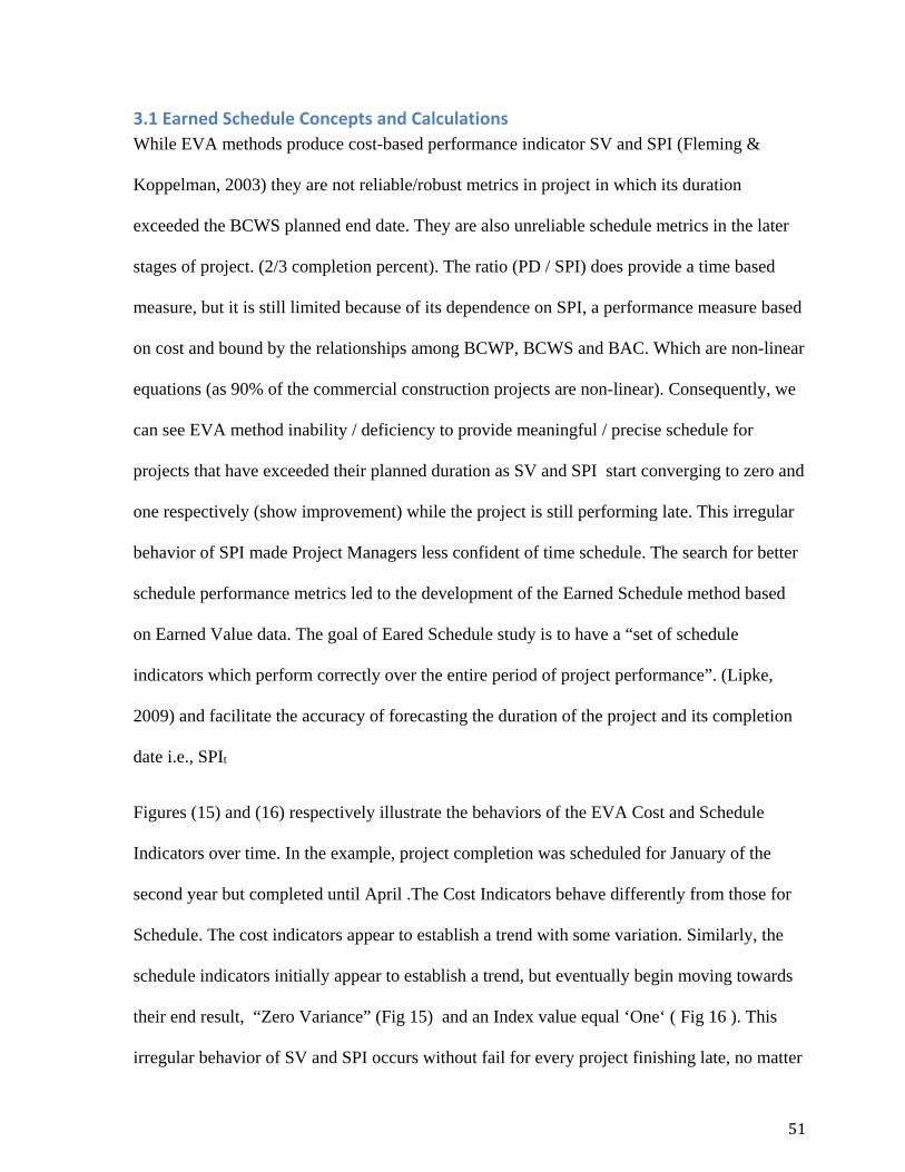
3.1 Earned Schedule Concepts and Calculations While EVA methods produce cost-based performance indicator SV and SPI (Fleming &
Koppelman, 2003) they are not reliable/robust metrics in project in which its duration
exceeded the BCWS planned end date. They are also unreliable schedule metrics in the later
stages of project. (2/3 completion percent). The ratio (PD / SPI) does provide a time based
measure, but it is still limited because of its dependence on SPI, a performance measure based
on cost and bound by the relationships among BCWP, BCWS and BAC. Which are non-linear
equations (as 90% of the commercial construction projects are non-linear). Consequently, we
can see EVA method inability / deficiency to provide meaningful / precise schedule for
projects that have exceeded their planned duration as SV and SPI start converging to zero and
one respectively (show improvement) while the project is still performing late. This irregular
behavior of SPI made Project Managers less confident of time schedule. The search for better
schedule performance metrics led to the development of the Earned Schedule method based
on Earned Value data. The goal of Eared Schedule study is to have a “set of schedule
indicators which perform correctly over the entire period of project performance”. (Lipke,
2009) and facilitate the accuracy of forecasting the duration of the project and its completion
date i.e., SPIt
Figures (15) and (16) respectively illustrate the behaviors of the EVA Cost and Schedule
Indicators over time. In the example, project completion was scheduled for January of the
second year but completed until April .The Cost Indicators behave differently from those for
Schedule. The cost indicators appear to establish a trend with some variation. Similarly, the
schedule indicators initially appear to establish a trend, but eventually begin moving towards
their end result, “Zero Variance” (Fig 15) and an Index value equal ‘One‘ ( Fig 16 ). This
irregular behavior of SV and SPI occurs without fail for every project finishing late, no matter
51

how late. This abnormal behavior of the schedule indicators with its misinterpretations and
misunderstandings weakens the initiative to broaden the acceptance and application of EVA.
Figure 15 Cost and Schedule Variances
Figure 16 Cost and Schedule Performance indices example
52
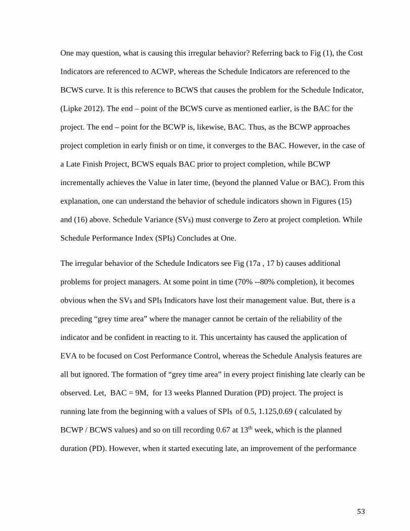
One may question, what is causing this irregular behavior? Referring back to Fig (1), the Cost
Indicators are referenced to ACWP, whereas the Schedule Indicators are referenced to the
BCWS curve. It is this reference to BCWS that causes the problem for the Schedule Indicator,
(Lipke 2012). The end – point of the BCWS curve as mentioned earlier, is the BAC for the
project. The end – point for the BCWP is, likewise, BAC. Thus, as the BCWP approaches
project completion in early finish or on time, it converges to the BAC. However, in the case of
a Late Finish Project, BCWS equals BAC prior to project completion, while BCWP
incrementally achieves the Value in later time, (beyond the planned Value or BAC). From this
explanation, one can understand the behavior of schedule indicators shown in Figures (15)
and (16) above. Schedule Variance (SV$) must converge to Zero at project completion. While
Schedule Performance Index (SPI$) Concludes at One.
The irregular behavior of the Schedule Indicators see Fig (17a , 17 b) causes additional
problems for project managers. At some point in time (70% --80% completion), it becomes
obvious when the SV$ and SPI$ Indicators have lost their management value. But, there is a
preceding “grey time area” where the manager cannot be certain of the reliability of the
indicator and be confident in reacting to it. This uncertainty has caused the application of
EVA to be focused on Cost Performance Control, whereas the Schedule Analysis features are
all but ignored. The formation of “grey time area” in every project finishing late clearly can be
observed. Let, BAC = 9M, for 13 weeks Planned Duration (PD) project. The project is
running late from the beginning with a values of SPI$ of 0.5, 1.125,0.69 ( calculated by
BCWP / BCWS values) and so on till recording 0.67 at 13th week, which is the planned
duration (PD). However, when it started executing late, an improvement of the performance
53
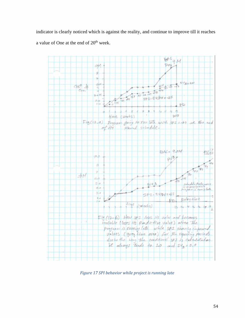
indicator is clearly noticed which is against the reality, and continue to improve till it reaches
a value of One at the end of 20th week.
Figure 17 SPI behavior while project is running late
54

3.2 Earned Schedule Measures and Indicators The concept of Earned Schedule (ES) is analogous to the concept of Earned Value. However,
instead of using cost for measuring Schedule Performance, the unit is “Time.” The
fundamental concept of ES is to determine the time at which the BCWP accrued should have
occurred; i.e., the time associated with point on the BCWS curve where PCWS equals BCWP.
The significance of the Earned Schedule Concept is that the associated schedule indicators
behave reliably throughout the entire period of project performance. Figure (18) below shows
the mathematical model of interpolation, and Figure (19) shows mathematical representation
Earned Schedule into Earned Value Analysis graphs.
Figure 18 Mathematical Model of Interpolation
55
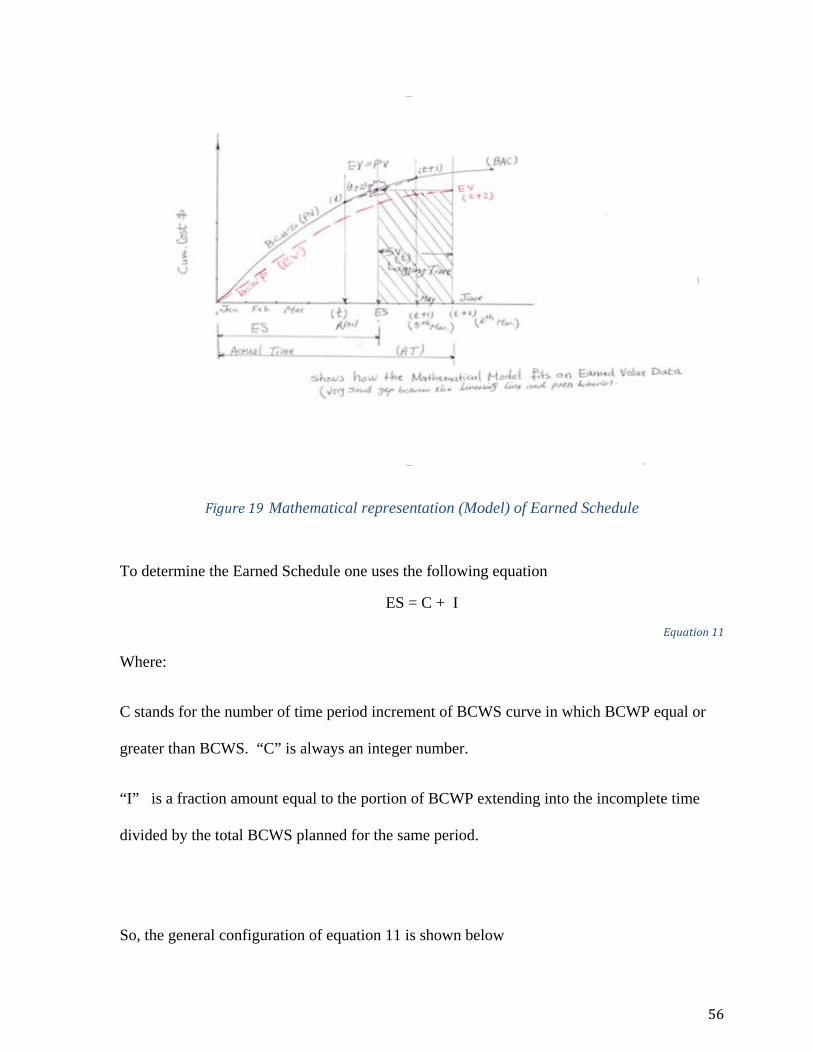
Figure 19 Mathematical representation (Model) of Earned Schedule
To determine the Earned Schedule one uses the following equation
ES = C + I
Equation 11
Where:
C stands for the number of time period increment of BCWS curve in which BCWP equal or
greater than BCWS. “C” is always an integer number.
“I” is a fraction amount equal to the portion of BCWP extending into the incomplete time
divided by the total BCWS planned for the same period.
So, the general configuration of equation 11 is shown below
56

ES = C + [ ( BCWP( t+2) - BCWS ( t) ) / ( BCWS ( t+1 ) – BCWS ( t ) ) ]…… ..
Equation 12
ES is computed as an interpolation process a shown in graphic representation in Fig (20).
Figure 20 Earned Schedule derived equations from EVA & S – Curves.
The value of time incremental (C ) is easily determined by counting the number of time
increments of the PMB that satisfy the condition, BCWP ≥ BCWS. The value of (I) is
calculated by employing the linear interpolation method for the (C+ 1 ) period of the BCWS
curve. The amount of BCWP extending into the (C+1) period is equal to the difference of
(BCWP) minus (BCWS), where (BCWS) is determined from the BCWS value associated with
period (C). The periodic amount of BCWS for period (C+1) is the difference BCWSc+1 minus
BCWS. The fraction (I) is calculated from the quotient of these two values as follow:
I = (BCWPt+2 – BCWSt ) / ( BCWS c+1 - BCWSt )
Equation 13
57

When determined, the two values (C and I) are added to become the value of ES.
So, ES = C + I
Where the units are in time periods, commonly months or weeks.
Using the ES measure, indicators are established which behave appropriately and analogously
to the cost indicators (CV and SPI):
Schedule Variance SVt = ES - AT
Equation 14
Schedule Performance Index SPIt = ES / AT
Equation 15
Where AT is the actual time, (referring to Fig 20 ) .
The Schedule Variance, SVt, is positive when the ES exceeds AT, and of course, is negative
when it lags. The Schedule Performance Index, SPIt, is greater than 1.0 when ES exceeds AT,
and is less than 1.0 when ES is less than AT. These proposed indicators are completely
analogous to the EVA Cost Indicators, CV and CPI. The proposed Schedule Indicators are
referenced to AT, similarly to the EVA Cost Indicators referenced to ACWP.
Referring back to Fig (20), the performance portrayed is of a project having schedule
performance lagging its plan. It can be observed that the vertical dashed line from the point on
the BCWS curve where BCWS = BCWP intersects the time axis at a point occurring
sometime in the month of “May “. The inset of the figure shows the calculation of ES and the
value for AT. The time period at which the BCWP accrued is reported, is the end of June,
58

AT = 6. The whole number component of ES, i.e, C, is associated with BCWS at the end of
April or month (4) the interpolated portion of ES, I, is spelled out in the inset of the Figure as:
I = [EV projected – PV April] / [PV May – PV April]
Where BCWP is larger than the BCES value for April, but smaller than the BCWS value for
May. Thus, the interpolation is made for May. Table 6 summarizes all these expressions
Method SPI IEACt
EVM BCWP (EV) /BCWS ( PV ) 1. AT+[ (BAC – EV) / BCWS avg. WR]
2. PD / SPI
3. AT + [(BAC – EV ) / EV avg. WR ]
ES ES / AT
Where ES = C + I
1. PD / SPIt
2. AT + ETC
ETC t =( TD – ES) / SPIt
Table 6 Summary of EVA and ES Performance Metrics
• AT: Actual time where PV and E V are reported
• WR: work rate that converts work into time.
• BCWS avg.: value is used when the program is expected to progress according to plan
BCWS avg. = BCWS cum / n
• BCWP avg. is used to depict performance that is expected to follow the current SPI
trend, BCWP / n.
• n: is the total number of time increments within AT.
• C: is the total number of time increment in which BCWP has been accomplished.
• I: partial time in which partial BCWP has been occurred within AT.
59

Now, let us check the viability of ES equation by assigning some hypothetical numerical
values and working out the calculations as shown in the following example.
Example 1 Assume we are reporting on the end of June in Fig (20). So, AT = June (6), with a
Corresponding BCWP of ($1000) assumed at reporting date. Which is the same value after
being projected horizontally on BCWS curve i.e., = $ 1000. So,
BCWS on April = $ 900;
BCWS May = $ 1100 and
PD = 7.0 Month. (Planned end).
Solving for I = [ 1000 -- 900 ] / [ 1100 -- 900 ] = 0.50 Month. EV has taken to accrue. So,
ES = 4 + 0.5 = 4.5 Month (total time)
SPIt = ES / AT ; 4.5 / 6 = 0.75
ETCt = ( 7 – 4.5 ) / 0.75 = 3.333 Month for work remaining, and
EACt = 4 + 3.33 = 7.33 Month
Now, using the same example but this time using EVA parameters,
We have BCWP = $ 1000 (As of reporting date), and BCWS = $ 1100 (as already
assumed). So,
SV = BCWP – BCWS
Using terms of volume of work or cost $1 =1 unit volume of work one gets:
60

SV = 1000 – 1100 = - 100
SV % = SV / PV as of date will be
SV% = 100 / 1100 * 100 = - 9 % decrease
Reporting date is June, which is 6th month. So,
0 .09 * 6 = 0.54 mon. late;
SV% = (0.54 – 0.5 ) / 0.54 * 100 = 7.407 % more time
SPI = BCWP / BCWS , 1000 / 1100 = 0.909
So, EAC = PD / SPI = 7 / 0.909 = 7.70 Month
The difference is ( 7.70 – 7.33 ) / 7.33 * 100 = 5 % more than ES est. time.
To demonstrate the concept of Earned Schedule further, let us consider the following example
Example 2 Considering the hypothetical data created for BCWS and BCWP. The data, along with the
calculated results for ES, i.e., SVt and SPIt are tabulated in table (7) below for early finish
project, and table (8) for late finish project respectively.
EVA method (January)
BCWS for month (Jan) = $ 106
BCWP for month (Jan) = $ 116
SV$ = BCWP – BCWS or SV$ = 116 – 106 = $ 10
A positive sign indicate progress ahead of planned.
61

SPI$= BCWP / BCWS, or SPI$= 116 / 106 = 1.095
A ratio over 1 indicates the project ahead of plan, good efficiency of time, the project team is
achieving. So,
IEAC = PD / SPI$, or IEAC = 12 / 1.095 = 10 .968
This imply a month less than planned.
ES method (January)
I = ( BCWP Jan – BCWS) / ( BCWS Jan – BCWS) ,
I= (116 – 0 ) / ( 106 – 0 ) = 1.094
ES = C + I,
ES = 0 + 1.094 = 1.094 Month.
SV t = ES – AT
SV t = 1.094 – 1 = 0.94 Month. ( project ahead of plan ).
SPI t = ES / AT, 1.094 / 1 = 1.094
So,* IEACt = PD / SPI t, IEACt = 12 / 1.094 = 10.968 mon. less than planned.
The forecasts obtained by either method are the same since the percent completion is less than
15%, and project is progress ahead of planned.
The star (*) above indicates the indicator IEAC t = PD /SPI t, has been used as the project is
progressing as planned. For more details, refer to table (6).
62
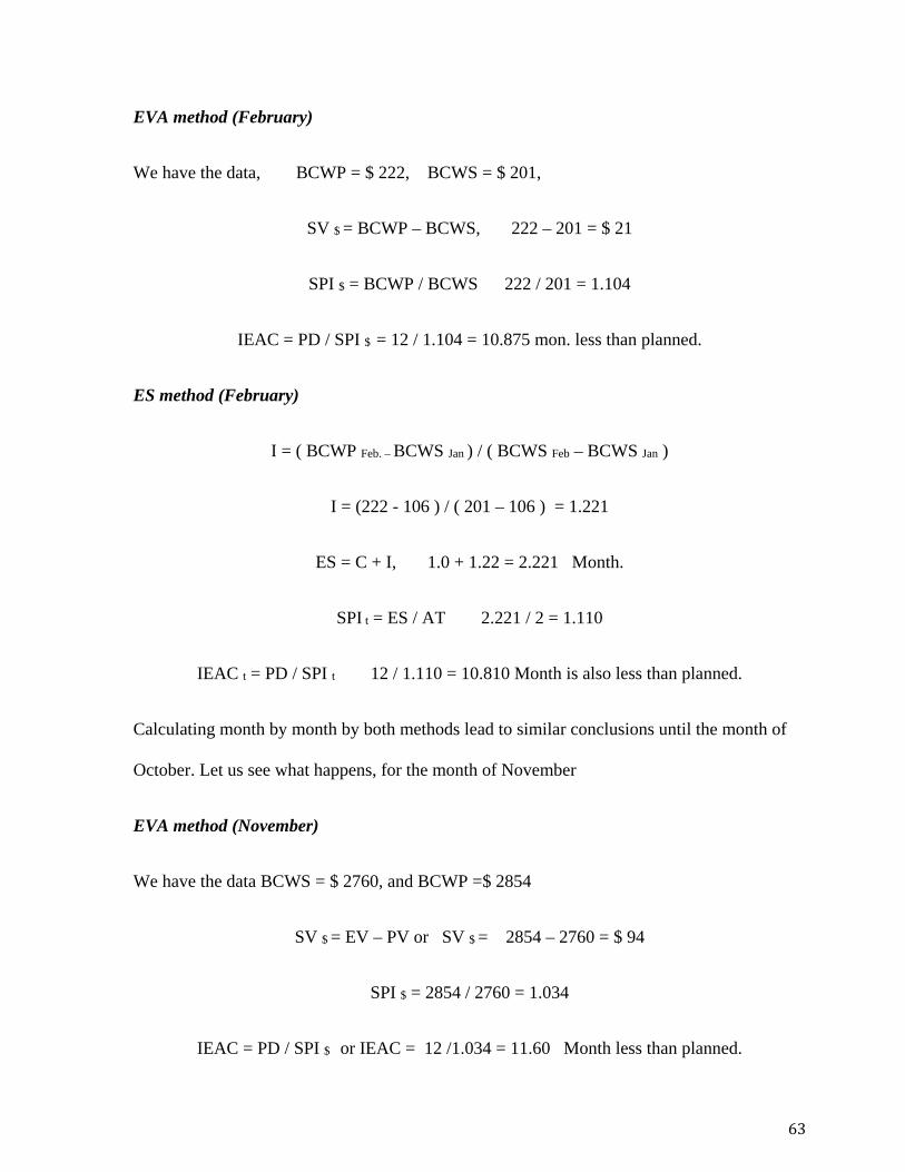
EVA method (February)
We have the data, BCWP = $ 222, BCWS = $ 201,
SV $ = BCWP – BCWS, 222 – 201 = $ 21
SPI $ = BCWP / BCWS 222 / 201 = 1.104
IEAC = PD / SPI $ = 12 / 1.104 = 10.875 mon. less than planned.
ES method (February)
I = ( BCWP Feb. – BCWS Jan ) / ( BCWS Feb – BCWS Jan )
I = (222 - 106 ) / ( 201 – 106 ) = 1.221
ES = C + I, 1.0 + 1.22 = 2.221 Month.
SPI t = ES / AT 2.221 / 2 = 1.110
IEAC t = PD / SPI t 12 / 1.110 = 10.810 Month is also less than planned.
Calculating month by month by both methods lead to similar conclusions until the month of
October. Let us see what happens, for the month of November
EVA method (November)
We have the data BCWS = $ 2760, and BCWP =$ 2854
SV $ = EV – PV or SV $ = 2854 – 2760 = $ 94
SPI $ = 2854 / 2760 = 1.034
IEAC = PD / SPI $ or IEAC = 12 /1.034 = 11.60 Month less than planned.
63

ES method (November)
I = (BCWP Nov. – BCWS Oct. ) / ( BCWS NOV – BCWS Oct. ),
I = (2854 – 2666 ) / ( 2760 – 2666 ) = 2
ES = 10 + 2 = 12 month
This means that Earned Schedule of 12 months’ work has been occurred in 11 months only.
SV t = ES – AT, or SV t = 12 – 11 = 1.0 Month less than planned.
SPI t = ES / AT, 12 / 11 = 1.091
IEAC t = PD / SPI t, or IEAC t = 12 / 1.091 = 11.0 Month, the job has been done!
The difference between two methods is for ES and EVA is
SV% = (11.6 – 11) / 11 * 100 = 5.45% less than EVA forecast.
Therefore, ES yields a more realistic and accurate time forecast than EVA
The resulting SVt and SPIt for each month are tabulated in table (7) and plotted in Figure (21)
below for early finish project. The resulting SV$ and SPI$ for each month plotted in Figure
(22) below for early finish project
64

Table 7 Early Finish Project Example 2
Figure 21 Comparison of SPI (t) & SPI ($) trend for Example 2
65
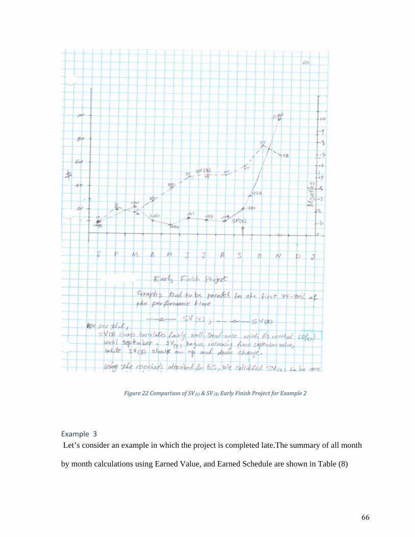
Figure 22 Comparison of SV (t) & SV ($) Early Finish Project for Example 2
Example 3 Let’s consider an example in which the project is completed late.The summary of all month
by month calculations using Earned Value, and Earned Schedule are shown in Table (8)
66

EVA method (January)
Considering (January) as beginning of the project, the data are,
BCWP cum = $100, and BCWS cum =$110,
SV$ = 100 – 110 = - $ 10 (minus sign indicates late progress).
SPI $ = BCWP / BCWS 100 / 110 = 0.9090
IEAC = PD / SPI $ 12 / 0.9090 = 13.20 Month.
EVA method (January)
I = ( BCWP Jan – 0 ) / ( BCWS Jan - 0 ) , ( 100 - 0 ) / ( 110 – 0 ) = 0.9090
ES = C+ I, 0+ 0.9090 = 0.9090 Month.
SV t = ES – AT, 0.9090 – 1 = - 0.09 Month late
SPI t = ES / AT, 0.9090 / 1 = 0.9090
So, IEAC = PD / SPI t, 12 / 0.9090 = 13.20 month.
Same values are expected to be identical for 15% completion only.
EVA method (February)
BCWP = $ 185, and BCWS = $ 205
SV $ = BCWP – BCWS, 185 – 205 = - $ 20
SPI $ = BCWP / BCWS, 185 / 205 = 0.900
IEAC = PD / SPI $, 12 / 0.900 = 13.34 Month.
EVA method (February)
I = (BCWP Feb – BCWS Jan) / (BCWS Feb – BCWS Jan),
I = (185 – 110) / (205 – 110) = 0.789
ES = C + I, 1+ 0.789 = 1.789 Month.
SV t = ES – AT, 1.789 – 2 = - 0.210 month delay in EV to occur as planned.
SPI t = ES / AT, 1.789 / 2 = 0.894
So, IEAC t = PD / SPI t, 12 / 0.894 = 13.420 Month. More than EVA method
67

Calculating month by month by both methods lead to similar conclusions until the month of November. Let us see what happens, for the month of December
In Dec. the last month of scheduled duration, the calculations of time duration are as follow:
EVA method (December)
EV = $ 2690 and PV = BAC = $ 2854
SV $ = BCWP – BCWS, 2690 – 2854 = - $ 164
SPI $ = BCWP / BCWS, 2690 / 2854 = 0.942
And IEAC = PD / SPI $ 12 / 0.942 = 12. 731 Month.
ES method (December)
BCWP Dec = $2690, and BCWS Nov = $2765
I = ( 2690 – 2765 ) / ( 2854 – 2765 ) = - 0.442
ES = 11 – 0.442 = 10.60 Month.
SV t = ES – AT, 10.6 – 12 = - 1.84 Month.
SPI t = ES / AT, 10.60 / 12 = 0.846
So, IEAC t = PD / SPI t, 12 / 0.846 = 13.60 Month which is more realistic than EVA forecast.
Now, solving for the delayed time the project undergoing, which starts on January of next year, say (2002), we have the following data,
EVA method (January 2002)
BCWP cum = $2695, and BCWS cum = BAC = $2854,
SV $ = BCWP – BCWS, 2695 – 2854 = - $159
SPI $ = BCWP / BCWS, 2695/2854 = 0.944
IEAC = PD / SPI $ 12 / 0.944 = 12.701 Month.
ES method (January 2002)
Here, we have no planned value yet to be used in the Baseline, as PV has already reached the BAC much earlier than BCWP reaches BCWS at the end of project.
So, using the Percent Complete ratio = Work done / Total work
68

BCWP = % complete * BAC,
So, ES = BCWP / BAC * PD , 2695 / 2854 * 12 = 11.45 Month.
SV t = ES – AT, 11.45 – 13 = - 1.5 Month, late from planned.
SPI t = ES / AT, 11.45 / 13 = 0.880
So, IEAC t = PD / SPI t, 12 / 0.880 = 13.636 Month.
EVA method (February 2002 delayed time)
The data are, EV =$ 2770, and PV = BAC =$ 2854,
SV $ = BCWP – BCWS, 2770 – 2854 = - $ 84
SPI $ = BCWP / BCWS, 2770 / 2854 = 0.970
IEAC = PD / SPI $ 12 /0.970 = 12.37 Month.
ES method (February 2002 delayed time)
ES = 2770 /2854 *12 = 11.64 Month.
SV t = 11.64 – 14 = - 2.35 Month. late
SPI t = ES / AT, 11.64 / 14 = 0.831
And IEAC t = PD / SPI t, 12 / 0.831 = 14.44 Month.
Considering the March the last month
EVA method (March 2002 delayed time)
The data are as follow;
BCWP cum = $ 2854, BCWS cum =BAC = $ 2854
SV $ = $ 0,
SPI $ = 1
IEAC = 12 /1 = 12 Month. meaningless ?
ES method (March 2002 delayed time)
ES = 2854 / 2854 *12 = 12 Month.
69
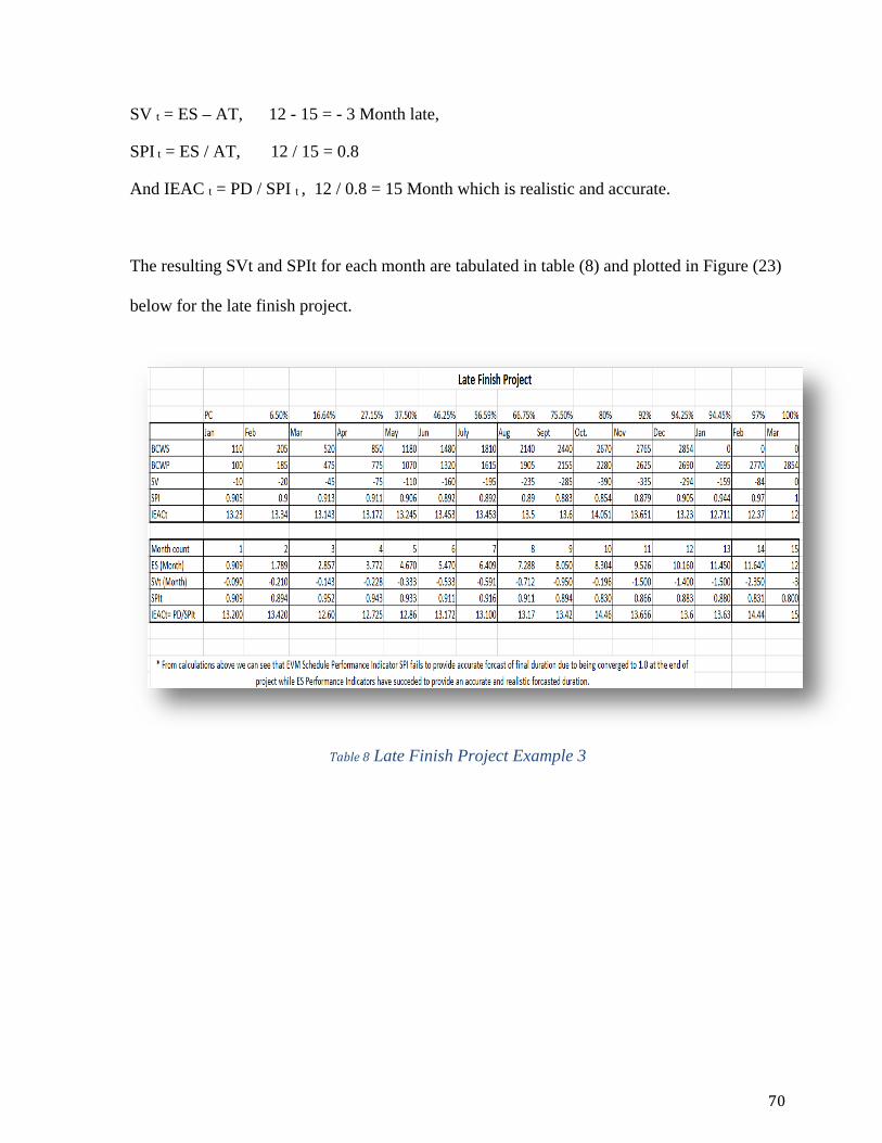
SV t = ES – AT, 12 - 15 = - 3 Month late,
SPI t = ES / AT, 12 / 15 = 0.8
And IEAC t = PD / SPI t , 12 / 0.8 = 15 Month which is realistic and accurate.
The resulting SVt and SPIt for each month are tabulated in table (8) and plotted in Figure (23)
below for the late finish project.
Table 8 Late Finish Project Example 3
70

Figure 23 Late Finish Project, Schedule Performance Comparison of example 3
71

Chapter 4 CASE STUDY
4.1 Earned Value Analysis, Earned Schedule and Building Information Modeling (BIM) Worcester Polytechnic Institute (WPI) is one of the US earliest technical universities. It was
founded in 1865 to create and convoy the latest science and engineering knowledge in ways
that are most beneficial to society. WPI’s founding motto for Lehr und Kuntz (Theory and
Practice) underlines its academic programs. for several years now, faculty and students in the
Civil and Environmental Engineering Department and in particular those involved in the
construction project management program, have been working together with college
administration through WPI’S project-oriented educational system to identify efficient uses
and implementation of Information Technology as a two-way avenue that enhances the
institution’s management information system for new and existing facilities .This activity is
now focusing on the use of Building Information Modeling (BIM ) as enabler for information
integration and more collaborative design, construction and operational process which has
been in the industry system since the early 1980s.The following is an overview concise
narrative of BIM and project management software process utilized in this mission.
The 3D model is useful for visualizing the shape instead of imagining it, quantifying the
construction materials, performing clash detection, creation of cost and time –phased 4D and
5D models in addition to calculating total cost of whole project components with 90%
accuracy to be incorporated with EVA and ES “S- curve”. Microsoft Project Planner 2013
software is useful for scheduling the work packages (including their assigned Budgeted Costs
of work packages along with Actual Spending amounts(ACWP) obtained from the project
records) after tabulating them with the same logical task precedencies and interrelationships to
72

be similar to what were used by the prime contractor in order to generate the Gantt chart,
critical path, network diagram, ending with S-curve diagram displaying cost time relationships
of the scheduled activities so that the EVA and its extension ES data (cumulative cost - time
values) would be captured from the S-curve. After this stage, it is possible/suitable to connect
the work with BIM tools, such as Navisworks software, and by phasing and integrating the
structural components of 3D model to their assigned construction time periods and costs 4D
and 5D models are created to reflect the physical progression of time- cost milestones to be
incorporated on S-curve. The 4D modeling helps the sub-contractors to detect visually any
error or discrepancy on the drawings prior to any phase extension, and to monitor the schedule
adherence during the construction phase, while 5D reflects the dynamic relation among the
three variables cost- time and scope and shows how a change of one variable affect the other
two variables in digital representations.
4.2 Parking Garage Facility In order to check the applicability/reliability of EVA and ES Schedule Performance Indicators
and time forecast duration metrics along with BIM 3D, 4D and 5D simulations on a real
project, a Parking Garage with Rooftop Athletic Fields with Synthetics Turf for Soccer at WPI
campus was chosen for this study as being of late completion projects.
Description of Facility
In late October 2011, WPI made a decision to build a $20M dollars, 536 cars one-way Parking
Garage Project with a rooftop Athletic Field with Synthetics Turf for Soccer, field Hokey,
Lacrosse, Rugby and Softball uses at WPI campus. The project includes a small section for
restrooms locker rooms, field storage and concession stands. The project was delivered under
a contractor-led Design Build System (DB – GMP contract). By Gilbane Building Company
73

(GBC) with guaranteed maximum price contract $ 20.0 M. to cover the cost of all materials,
design, labor, equipment, supervision, insurance and all other aspects considered necessary to
construct the facility within nine months only. Construction was started as scheduled on late
May, 2012. The Parking and was completed and delivered /occupied in late January 2013,
whereas the playing fields were substantially completed in early summer (May, 28, 2013)
because the owner’s approval to defer the installment of Synthetic Turf after the severe
winter months when better weather condition (Temperature and Humidity) allow for
Synthetic Turf to be installed as recommended by manufacture.
4.3 Work procedures for Earned value Analysis and Earned Schedule This section shows how data was collected and processed.
4.3.1 Data collection and Scheduling with Microsoft Project 2013 The extraction of input data and scheduling took considerable time as the records of (budgeted
costs and actual spending costs) where recorded three years ago and were not easily
referenced in the format for direct EVS and ES calculations. Therefore the original
information as collected needed to be processed carefully and judicially to allow for its valid
use for this study. Then the first step is composing the main activities (work packages) in such
a way to be of analogous order to that used by the prime contractor records, and referring their
pertinent sub-activities to each of them as well (See Table 9). The way to configure the Work
Breakdown Structure (WBS) is shown in Figure (24) which represents a reference of planning
and scope of work making it clear and tangible..
74

Figure 24 Parking Garage Work Breakdown Structure
75

Table 9 Parking Garage Data for EVA & ES Analysis
After WBS was set, the scheduling of activities (work packages) was conducted using
Microsoft Project 2013 software Figures 25 and 26 show Gantt charts for on time and late
completions respectively.
76

Figure 25 Gantt Chart on time completion
Figure 26 Gantt chart late completion
Figures 27 & 28 display the S-curves for BCWS and ACWP for the on time completion and
late completion respectively
77

Figure 27 on time completion S-Curves for Budgeted Cost and Actual Cost
78

Figure 28 Late completion S-Curves for Budgeted Cost and Actual Cost.
The above curves were generated by Microsoft Project 2013
79

4.3.2 Earned Value Calculation The target is to quantify the earned value of work done for each month of work progress
represented in figure (28) of late completion of the same schedule. The Budgeted Cost of
Work Performed (BCWP) is usually calculated by one of the previously mentioned BCWP
equations listed in Chapter 2 such as;
BCWP = % complete x BAC
Where: Percent complete = (Budgeted units – Units to complete) / Budgeted units.
By this Equation, the BCWP is measured as milestones. However, by examining the behavior
of S-curves for Budgeted cost and Actual cost Figure (28) and reading the projected values of
cumulative monthly cash flows on vertical axis on any interval of time, one can find that the
progressive curve of ACWP is almost identical to the BCWS curve (with a very small gap)
which means the work (or the payments were made as projected) was progressing as budgeted
costs. So, that gap (time difference in terms of money) could be considered having no
influence, and could be ignored in project management, (Mubarak 2010).This means that the
(BCWP) of work in progress is the same as (ACWP) indicating to the owner that the
budgeting is adequate.
So, one can infer that BCWP = ACWP. This embodies the essence of GMP contract
implementation by both the contractor and the owner, i.e., (no savings made from hard cost).
Now, we have two sets of values:
1. Cumulative Budgeted Costs as of BCWS.
80

2. Cumulative Cost (ACWP) as a (BCWP) for each time interval of project Planned Duration
(PD).
From these two sets of values, the EVA and its extension ES parameters (Indicators and cost
variances) are derived / calculated as shown in the following table 10. By comparing the
calculated or forecasted IEAC resulted from both methods [EVA and ES] with basic CPM
duration or the Baseline Planned Duration (PD), a range of time variations from these two
methods visually and quantitatively are noticed. The realistic one that better represents the
actual time consumed by the project to get completed would be considered as the true total
project duration. It also shows which indicator is more reliable to be adopted for tracking and
calculating (forecasting) the IEAC of the project. (has no convergence to One at the end of the
project, and behaves analogous to CPI trend). Keeping in mind that the CPM course of
activities has not been changed during the construction phase.
Below is the actual numerical values used in determination of Earned Value and Earned
Schedule indicators of case study project lifecycle.
EVA calculations (May 2012) Considering Month (May 2012), the data is PV cum = $ 500,000 and EV cum = $ 480,000
% Complete = 480000 / 15196721 * 100 = 3.15 %
SV $ = BCWP – BCWS, 480000 – 500000 = - $ 20000
SV$ % = SV / BCWP, - 20000 / 480000 = - 0.004 %
SPI$ = BCWP / BCWS = 0.960
IEAC = PD / SPI $, 9/ 0.960 = 9.375 Month.
ES calculations (May 2012) I = ( BCWP May – BCWS ) / ( BCWS May- BCWS ) , ( 480000 – 0 ) / ( 500000 – 0 ) = 0.96
81
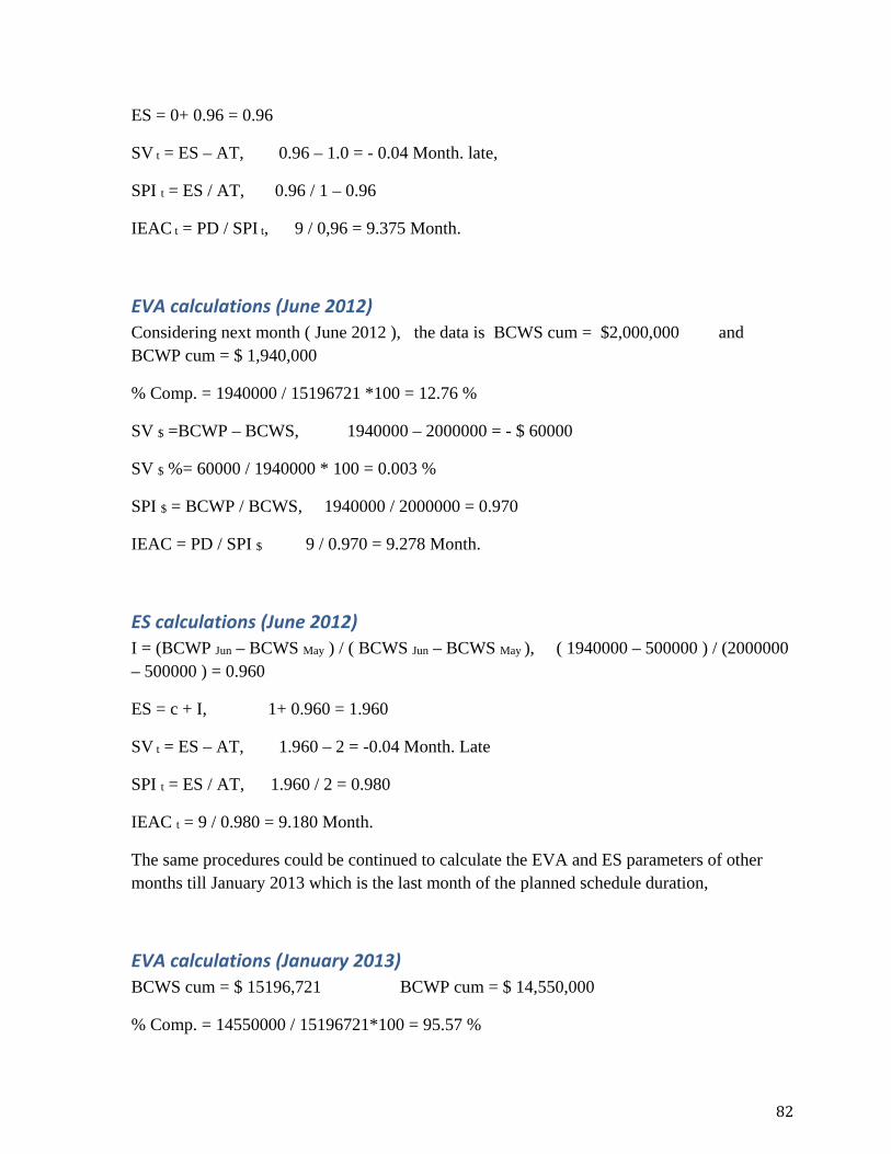
ES = 0+ 0.96 = 0.96
SV t = ES – AT, 0.96 – 1.0 = - 0.04 Month. late,
SPI t = ES / AT, 0.96 / 1 – 0.96
IEAC t = PD / SPI t, 9 / 0,96 = 9.375 Month.
EVA calculations (June 2012) Considering next month ( June 2012 ), the data is BCWS cum = $2,000,000 and BCWP cum = $ 1,940,000
% Comp. = 1940000 / 15196721 *100 = 12.76 %
SV $ =BCWP – BCWS, 1940000 – 2000000 = - $ 60000
SV $ %= 60000 / 1940000 * 100 = 0.003 %
SPI $ = BCWP / BCWS, 1940000 / 2000000 = 0.970
IEAC = PD / SPI $ 9 / 0.970 = 9.278 Month.
ES calculations (June 2012) I = (BCWP Jun – BCWS May ) / ( BCWS Jun – BCWS May ), ( 1940000 – 500000 ) / (2000000 – 500000 ) = 0.960
ES = c + I, 1+ 0.960 = 1.960
SV t = ES – AT, 1.960 – 2 = -0.04 Month. Late
SPI t = ES / AT, 1.960 / 2 = 0.980
IEAC t = 9 / 0.980 = 9.180 Month.
The same procedures could be continued to calculate the EVA and ES parameters of other months till January 2013 which is the last month of the planned schedule duration,
EVA calculations (January 2013) BCWS cum = $ 15196,721 BCWP cum = $ 14,550,000
% Comp. = 14550000 / 15196721*100 = 95.57 %
82

SV $ = BCWP – BCWS, 14550000 – 15196721 = - $ 646,721
SV $ % = - 646,721 / 14,550,000 *100 = - 4.5 %
SPI $ = BCWP/ BCWS, 14550000 / 15196721 = 0.957
IEAC = PD / SPI $ 9 / 0.957 = 9.4 MON.
ES calculations (January 2013) I = (BCWP Jan – BCWS Dec ) / ( BCWS Jan – BCWS Dec ),
I= (14550000 – 14300000) / (15196721 – 14300000) = 0.278
ES = C + I, 8 + 0.278 = 8.278 Month.
SPI t = ES / AT, 8.278 / 9 = 0.9197
IEAC t = PD / SPI t , 9 / 0.9197 = 9.785 Month.
The Calculation continues for delayed time execution considering Feb. 2013
EVA calculations (February 2013) Here BCWS ~ BAC much earlier than BCWP approaches BCWS on the Baseline, and we have no more BCWS cum values on the Baseline planned duration while BCWP cum still achieving incremental values with time from work remaining.
So, using % Comp. equation to calculate the performance of project during the late completion time.
BCWS cum = $ 15,196,721 BCWP cum = $ 14,711,680
% Comp. = 14711680 / 15196721 *100 = 96.80 %
SV $ = BCWP – BCWS 14711680 – 15196721 = - $485,041
SV % = - 485041 / 14711680*100 = - 3.2 % ( Deviation)
SPI $ = BCWP / BCWS, 14711680 /15196721 = 0.968
IEAC = PD / SPI $ 9 / 0.968 = 9.300
ES calculations (February 2013) ES = 96.8 / 100 * 9 = 8.712 Month.
83

SV t = ES – AT, 8.712 – 10 = - 1.287 Month. late
SPI t =ES / AT, 8.712 / 10 = 0.871
IEAC = PD / SPI t 9 / 0.871 = 10.33 Month.
The calculation procedure is similar for the next months March and April 2013. For the month of May 2013
EVA calculations (May 2013) BCWS cum = BAC = $ 15,196,721
BCWP cum = BCWS cum = BAC = $ 15,196,721
% comp. = 100 %
SV $ = 0, SPI $ = 1, IEAC = PD /SPI $, 9 / 1 = 9 Month. ( meaningless)
ES calculations (May 2013) ES = 9 ( mon)
SV t = ES – AT, 9 – 13 = -4 Month. late
SPI t = ES / AT, 9 / 13 = 0.692
IEAC t = PD / SPI t, 9 / 0.692 = 13 mon. which is realistic, meets the Baseline/ (CPM).
The calculations for the entire project under both methods are summarized in Table 10
Table 10 Comparison between EVA final duration forecast vs. ES final duration forecast.
84

The resulting SVt and SPIt for each month are plotted in Figure (29) below
Figure 29 Comparison of Performance Indices SV$ vs. SVt and SPI$ vs. SPIt
85

4.3.3 BIM Integration The BIM model was created with Revit 15 Architectural and Structural tool. This software
program allows to accurately create a 3D model of the structure of the parking garage. The
model was The model was created using: 1) the precast structural subcontractor BIM model,
2) 2D construction shop drawings and sketches, 3) information and documentation provided
by the design-builder for this project. The Model was developed at a level of development
(LOD) 300 in which Model elements are modeled as specific assemblies which are accurate in
terms of quantity, size, shape, location. This level is similar to Design Development. It
included objects for the majority of the bid packages. The time schedule was provided by the
contractor in pdf format and it served as a guide to create a new time schedule using critical
path method software (Microsoft project 2013).
3D model The Revit Structural model started by setting up the different levels and grid lines. The grid
lines, which mimicked the structural drawings gridlines, were used to help provide a reference
for the different aspects of the structure. The attached 2D drawing, Figure (30) shows the
plan view of the garage level of the model with grid lines. Levels depict each different floor in
the structure. The levels included the subfloor or soil level. Level one which is the garage
level, and the second level which shows the athletic fields. These boundaries set up the basis
for creating the structural components of the building. As there are varying soil conditions
throughout the base of the garage, both deep and shallow foundations had to be used (size and
shape chosen identical to 2D drawings provided by the prime contractor). The piles were
inserted at each gridline intersection, similar to the architectural drawings. In areas where
there was bedrock closer to the surface, footings with a smaller surface area were used. While
86

pressure Injected Footings (PIFFs) had been used to reach the deeper depths where the soil
layers had a lower bearing capacity. The foundation was then finished by adding a foundation
wall on the perimeter to help support the interior structural shearing walls. A compacted
backfill and a two-binder asphalt layer were laid down on the top of the footing. Fig. (31)
shows 3D rendered image of a deep foundation piles under the foundation floor from the BIM
model. After the foundation was solidly built, the main components of the garage were added.
This started by putting columns on the garage level. For maximum ventilation, much of the
garage level was left open and walls were erected in only two of the four sides of the parking
garage. On the other side of the structure, steel girders were placed up against the edge of the
garage to support the upper level. Then precast concrete I beams were inserted and double Tee
beams as well as the girder to support the roof structure of the garage ending the
superstructure construction main components
.
Figure 30 Parking Garage Plan View
87

Figure 31 3D model of piled deep foundation (Alvarez & Gomez 2013)
Later on, in the project certain circumstances came into play. The school expected the project
to be completed in early January 2013 without getting deep into the winter months weather.
The main problem with cold weather was that the synthetic turf could not be sewn on the field
if the temperature was less than 45 degree Fahrenheit. This was a major challenge since it is a
five week process that was originally scheduled to take place in early December. As
construction progressed into the latter part of the schedule, it was determined that the most
practical option was to have parking garage completed by the early January, 2013 as
originally planned but the athletic turf should be executed in late in the spring under warmer
weather conditions and complete the project As of January 2013 until May 29, 2013. (Actual
completion date) .So, the project has recorded four months delay upon the pre- approval of the
owner.
88

Figure 32 Precast Double Tee Roof concrete slab (Alvarez & Gomez 2013)
The athletic field was built with a combined set of layered materials including cement screed
mortar reinforced with steel mesh was put in place as a base. Then followed with water proof
membranes and two layers of graded gravel to work as water drainage under the synthetic turf.
These layers were modeled by adding a floor with multiple layers. These layers included a sub
base, filter fabric gravel, sand and a top layer of grass as seen in the Figure 33. Outside the
turf there were two sidewalks that run the length of the field
Figure 33 layered system for the athletic field (Alvarez & Gomez 2013)
89
4D model A 3D model can be phased to display the gradual progress of construction. A 4D model list
generated when each phase is combined with the actual dates of execution of that phase where
the complete shape, materials, and quantification are made available at that phase. This 4D
model is created by integrating Microsoft Project 2013 modified scheduled work packages
with the 3D BIM model components (sub-structure and super structure) that was originally
scheduled to handing over in early January 2013. But as mentioned earlier, due to bad weather
condition encountered the layout of synthetic turf, the schedule has been modified to end on
May 2013. Therefore, by inputting the modified project schedule (Finish-Start relationships)
for late completion, we can view each major construction milestone in the form of time
phased - cost as it was being built. Figures (35 & 36) below represent different phases of the
4D model. This action helps the subcontractors to check their models before/during
construction course for clashes if any. Moreover, the owners need to visualize the changes
happened at site and track the progress of work with associated cash flow and to arrange
mitigating any risks may arise with financial institution funding the project. Now each viewed
specific phase could be superimposed to the Project Management Baseline or S-curve of
project that was developed by EVA and ES as shown in Figure (37) to get the full integrated
benefit of utilizing BIM with EVA and ES method for involved stakeholders to track the time
and cash flow performance of project. This is the missing link through which the owners,
contractors and all stakeholders can make effective implementation of how BIM tools could
be merged with EVA and ES to track the progress of project.
90

Figure 34 4D model of construction progress (Abdulahad & Zabeti 2014)
Figure 35 4D model (Alvarez & Gomez 2013)
91

Figure 36 Time Cost & Scope Integration (Abdulahad & Zabeti 2014)
4.4 Case Study Results and Outcomes The following are the main results and outcomes derived from this case study
1. The research shows that the Schedule Variance SVt ( -4 ) which means (4) months late
is realistic, while EVA Schedule Variance SV$ = 0, and Schedule Performance Index
SPI $ converges to 1.0 . The SPIt = 0.692 (at month 13) means a deviation of 30%
from planned schedule had been taken place.
2. Earned Schedule shows that total project forecasted duration Indicator IEACt is (13)
months while Earned Value Indicator IEAC still shows (9) months only. Which is
unrealistic, thus misleading the owner expectations as to the date of completion and
preventing early discussion about the impact of a delay.
92
3. Earned Schedule (ES) Indicator IEACt for total duration is found to be identical to the
critical path method (CPM) duration or Baseline Planned Duration (PD), more
accurate than EVA, and directly correlated to it.
4. When two values of SPI$ and SPIt are found equal to each other exactly, planned and
actual performance of work progress are also equal on that period of time. (This is
happened only one time).
5. Earned Schedule (ES) measures the time in units of time (days, weeks, months), while
EVA makes assessment of time performance based on dollar value or cost value,
which makes it difficult to interpret, and match the variance with CPM of the project.
6. Earned Schedule (ES) could be applied on any time interval of project life-cycle, and
not only to the whole project duration which makes it very effective to track the
schedule performance of the project.
7. Earned Schedule (ES) more often eliminates the formation of gray time area at 70 -80
% completion (assessment distortion).
8. The work presented in this study allowed the researcher to explore the practical and
educational implications of using BIM models incorporated with Earned Value
Management Method in different aspects of design and construction process at WPI.
The researcher found that ;
BIM is a great way to visualize different design options .These models should be
used more often in design –build projects to help the client understand what the
different options will look like instead of trying to imagine them.
BIM can be used as a way to check estimates by quantifying the material from the
model.
93

BIM can track the project milestones in phases to help foresee the progress of
project throughout construction.
5D model explicitly displays the dynamic correlation among the three variables
Scope- Time and Cost in a clear visual fashion facilitating the understanding of the
impact that each variable has on the other two variables as well as on the
communication among the project participants.
The creation of the LOD 300 model brought out several modeling issues mainly with
regards to ;
- Interoperability.
- Extraction of information from 2D drawings design implications.
- Construction simulation.
- Fully integrated 5D and 6D modeling
- Better understanding and control of granularity (LOD) in the modeling.
- Granular Contains Transference of Experience to course and project work
(Construction Project Management and BIM courses).
94

Chapter 5 Final Conclusions and Recommendations
The following overall conclusions are derived from this study
1. Earned Schedule (ES) could be applied at any stage to assess the progress of work at
any time interval and not only to forecast the entire project duration, in units of time.
2. Earned Schedule (ES) uses the same data of Earned Value Analysis ( EVA) concept,
so it could be considered as an extension of EVA.
3. Earned Value Analysis (EVA) fails to give accurate / reliable Schedule Performance
terms for late completion projects, while it is accurate only for Cost performance
terms, (CV and CPI ).
4. Due to its accuracy, and realistic results, ES should always be used in conjunction with
EVA to assess Schedule Performance in order to protect the rights of owners to claim
for unjustified delay by the contractor(s) if any, and to seek the fair allocation when
“liquidated damages” clauses exit in the contract.
5. Recommendation; Specific to this study, SPI$ was figured to be already floated from
the beginning of the project and not a correct indicator(forecaster) up to 15%
completion, which need to be verified by further study.
6. Further BIM research need to be conducted using BIM such as Navisworks software to
solve the very congested fast track schedule to create more realistic 4D simulation.
95

BIBILOGRAPHY “A Guide to the Project Management” Project Management Institute (PMI, 2000).Project
Management Institute Publications.
Abba, W.F. (1999), “Beyond communication With Earned Value”. Project Management Institute Annual Seminar/symposium. New Orleans,16-18th oct. pp.2-6
Abba,W.F (1995) “ How Earned Value go to prime time, a short look back and a glance ahead ”. www.pmi-cpm.org Retrieved 2006
Abdulahad, M. and Zabeti,M. Term Project,( Fall 2014)WPI Parking Garage &BIM Integration. Term project presented to Professor Salazar, Guillermo.
Alukas, J. (2008), ACCE International Transactions “Earned Value analysis- why it does not work for Schedule Performance”.
Bruchey, W., (September 2012). “A Comparison of Earned Value and Earned Schedule Duration Forecast Methods on Department of Defense Major Defense Acquisition programs. http://calhoun.nps.edu/handle/10945/17329
Christensen D. S (Dec.2011), “ The Costs and Benefits of the Earned value Management process”.
http://www.tandfonline.com/doi/abs/10.1080/10157891.1998.10462568?journalCode=uzpa20#
Crumrine, Kevin T. Captain, U.SAF. A Comparison of Earned Value Management and Earned Schedule As Schedule Predictors on DoD ACAT I Programs. The Measurable News, 2013, http://earnedschedule.com/Docs/Crumrine%20Article%20-%20Measurable%20News%20(May%202013).pdf
Czarnigowska, A.’ ( 2008), “ Earned Value Method as a Tool for Project Control,” Lublin university of Technology,20 -618
Earned Value Management Implementation Guide, DoD Oct, 2006 http://acqnotes.com/acqnote/tasks/dod-earned-value-management-guide
Fleming and Koppelman ( 2002), “Earned Value Project Management” PMI (Earned Value Body Of Knowledge), PM network.
Fleming and Koppleman , “Earned Value Project Management” (2nd Edition) Project Management Institute, Newton Square, PA Pennsylvania, 2000
Fleming and Koppelman (1994c). “The Essence of Evolution of Earned Value” Cost Engineering. Vol. 36 No.11 November.pp21-27
Fleming and Koppelman , (June 2009),”The Two Most Useful Earned Value Metrics,” the CPI and TCPI. PM World Today. 2nd edition.
96

http://static1.1.sqspcdn.com/static/f/702523/9242593/1288743398867/200812-Fleming.pdf?token=QL7U4g9hJCRMtj6lQhYQ0%2FoPkRc%3D
Fleming and Koppelman, ( 1996), “ The Earned Value Body of Knowledge”. PMNET Work. Vol. 10 No. 5 May. “ Cost /Schedule Techniques for Building Projects in Australia”. http://webcache.googleusercontent.com/search?q=cache:PHtsopb_2QkJ:www.dtic.mil/cgi-bin/GetTRDoc%3FAD%3DADA402982+&cd=2&hl=en&ct=clnk&gl=us
Fleming and Koppelman, ( July 1998), “ Earned Value Project Management”. The Journal of Defense Software Engineering. http://admindeproyectos2do2011.googlecode.com/svn/trunk/Templates/Earned%20Value%20-%20A%20powerful%20tool.pdf
Fleming, Q.W.(1999). Cost/Schedule control System criteria. The management Guide to C/SCSC. Probus, Chicago http://www.stsc.hill.af.mil/crosstalk/frames.asp?uri=1998/07/value.asp
Harrison, F. and Lock, D. (4th edition, 2004) “ Advanced Project Management”. Gower Publishing Limited, Aldershot, UK.
Hecht, L. (2007/8). “ A Case Study of Earned Schedule to do Prediction,” The Measurable News, pp 16- 18, Winter.
Henderson, K. (2004). “Further Development in Earned Schedule,” The Measureable News, pp 15 – 22, Spring2004.. http://www.microplanning.com.au/wp-content/uploads/downloads/2011/10/Further-Developments-in-Earned-Schedule.pdf
http://www.baz.com/kjordan/swse625/htm/tp-py.htm
Humphreys, G., (2001), Earned Value Analysis , ISBN 0-9708614-0-0
Lanner, D., 2004 “ Earned Value For Project Managers” http://www.leaderhelper.com/Tools/EarnedValueManagement-Binder.pdf
Lipke, W. (2003), “Explanation of Earned Schedule” www.earnedschedule.com and
http:Sydney.pmichapters-australia.org.au/
Lipke, W. (2013). “Schedule Is Different”. The Measurable News, Summer, 2003 pp. 31-34
Lipke, W. (January 2011), “Earned Schedule performance Analysis from EVA Measures”. Second Edition 2011. Mc Grow Hill Professional Publishers.
Lipke, W.,. (2012). “Applying Earned Schedule to Critical Path analysis and More”. PM World Journal Sept. www.earnedschedule.com
Marshall, R. A 2007, “ The contribution of Earned Value management to project success of contracted efforts. Journal of contract management 2007. http://www.ncmahq.org/files/articles/jcm07_pp21-33.pdf
97

Mowery, B. MPM, PMP ( paper 2012), CSC, “ Earned Schedule; From Emerging Practice to Practical Application,” www.billymowery.com/Publications.htm
Mubarak, Saleh. “Construction Project Scheduling and Control”. John Wiley & Sons. 2010. 2nd edition.
Nagrecha, S., 2002, “ An Introduction To Earned Value Analysis,”. March 16 http://www.pmiglc.org/comm/articles/0410_nagrecha_eva-3.pdf
Nguyen, N.M. (1993). “Cost/Schedule Control in Project Management: A Canadian Approach” Project Management Annual Seminar/Symposium San Diego, 1-7th October. Pp178-186.
Paula, A., and Sylvestre, C.,( April 25th ,2013) Major Qualifying Project Report,( WPI), Construction Management and Foundation Design for WPI Athletic Rooftop parking Garage.
Project Management Book Of Knowledge (PMBOK 4th edition , December 2008 PMI).
Project Management Book Of Knowledge (PMBOK 5th edition, May, 2013 PMI).
Project Management Institute (2011) “ The Earned Value Management “ ( 2nd edition)
Rodrigues, Alexandre ( October 2010), “ Effective Measurement of Time Performance using Earned Value Management,” A proposed modified version for SPI tested across various industries and project types.. https://pmqlinkedin.files.wordpress.com/2011/05/effective-measurement-of-time-performance-using-earned.pdf
Rose, Kenneth H. ( Mar,1,2011 ), “Earned Value Project Management 4th edition p. 103” Project Management Journal, Vol. 42 Issue 3 page 103 Apr. 2011
Salazar G., Conron, C, “ Introduction of Objected Software into Civil Engineering Curriculum through Undergraduate Projects at WPI,” proceedings of the ASEE, Engineering Design Graphics Division 65th . Midyear conference, Berkely,CA, January 5, 2009.s
Salazar, G., Álvarez, S., Gomez, M., 2013,” Development of a 5D Case Study on The Design and Construction of Parking Garage with a Rooftop Athletic Fields at the WPI Campus, Worcester, MA”. 5D Conference Konztanz, Germany
Vandevoorde, S., Vanhoucke, M., “A Comparison of Different Project Duration Forecasting Methods Using Earned Value Metrics”. Project Management Publications . www.elsevier.com/locate/ijproman.
Turner, J.R. (2008, 3rd edition). “The Handbook of Project-Based Management – Improving the
Process for Achieving Strategic Objectives”. McGraw-Hill, London. Wilkens, T.T. (1993). “ An Effective Model for Applying Earned Value to any Project” San Diego,
1-7th October. Pp 170-177.
98

Young P.E. (April 1997), “Use of Earned Value management to Mitigate Software Development Risk” (online 2003) available.
99

LIST OF ACRONYMS AND ABBREVIATIONS ACWP ACTUAL COST OF WORK PERFORMED
ANSI AMERICAN NATIONAL STANDARD INSTITUTE
AT ACTUAL TIME
AT&L ACQUISITION, TECHNOLOGY AND LOGISTICS
ATE ACTUAL TIME EXPENDED
BIM BUILING INFORMATION MODELING
BAC BUDGET AT COMPLETION
BCWP BUDGETED COST OF WORK PERFORMED
BCWS BUDGETED COST OF WORK SCHEDULED
BCWSav AVERAGE COST OF WORK SCHEDULED
BCWSCum CUMULATIVE COST OF WORK SCHEDULED
CPM CRITICAL PATH METHOD
CPR CONTRACT PERFORMANCE REPORT
C/SCSC COST/SCHEDULE CONTROL SYSTEM CRITERIA
DID DATA ITEM DESCRIPTION
DoD DEPARTMENT OF DEFENCE
ES EARNED SCHEDULE
EVA EARNED VALUE ANALYSIS
EVav AVERAGE EARNED VALUE Evcum CUMULATIVE EARNED VALUE
100

EVM EARNED VALUE MANAGEMENT
EVMIG EARNED VALUE MANAGEMENT IMPLEMENTATION GUIDE
EVMS EARNED VALUE MANAGEMENT SYSTEM
FD ACTUAL FINAL DURATION
IEAC(t) EV INDEPENDENT ESTIMATE AT COMPLETION - EV method
IEAC(t) ES INDEPENDENT ESTIMATE AT COMPLETION - ES method
IMS INTEGRATED MASTER SCHEDULE
PD PLANNED DURATION
PMB PERFORMANCE MANAGEMENT BASELINE
PV PLANNED VALUE
SPI EVA SCHEDULE PERFORMANCE INDEX
SPI(t) Earned SCHEDULE PERFORMANCE INDEX
WBS WORK BREAKDOWN STRUCTURE
WR WORK RATE
101