Project Duration Forecasting … A Comparison of …earnedschedule.com/Docs/Project Duration...

2009, Issue 224 The Measurable News

Project Duration Forecasting … A Comparison of Earned Value Management Methods to Earned Schedule

By Walt Lipke, Member of Oklahoma City Chapter, Project Management Institute (USA)

AbstractEarned value management (EVM) methods for forecasting project duration have been taught in training courses and used by project managers for four decades. These EVM methods are generally considered to be accepted practice, yet they have not been well studied and researched as to their pre-dictive capability. Using real project data, this article examines and compares the duration forecasts from four EVM methods to the earned schedule prediction technique.

During Spring 2003, the concept of earned schedule (ES) was introduced, dem-onstrating the possibility of describing schedule performance in units of time

(Lipke, 2003). ES facilitates time-based analysis of the schedule employing uniquely the earned value management (EVM) measures of cost. One year subsequent to the publication of ES, the concept was extended to include project duration forecasting (Henderson, 2004). Henderson put forth two equa-tions for forecasting the final duration for a project; one of which is used in this study.

From 2004 to 2007, two independent papers were published investigating the capability of the ES fore-casting method. One article written by Lew Hecht describes, positively, the usefulness of ES in a case study of a single US Navy project (Hecht, 2007–2008). The second article is a comprehensive exami-nation of the capability of ES. The research team of Vanhoucke and Vandevoorde applied a simulation method for assessing the performance of two EVM-based methods and ES in forecasting project dura-tion (Vanhoucke and Vandevoorde, 2007). A portion of the Vanhoucke and Vandevoorde paper has been updated and published in the Winter 2007–2008 is-sue of The Measurable News (MN) (Vanhoucke and Vandevoorde, 2007–2008). The conclusion from the MN paper and its parent indicates “The results …confirm…that the Earned Schedule method outper-forms, on average, the other forecasting methods.”

Although the results of the research performed by Vanhoucke and Vandevoorde are well regarded, there remains the question of whether the simula-

tion technique is truly representative of real project circumstances. Likewise, the case study testimonial, while strongly supportive of the use of ES indicators and forecasting, is inconclusive in broadly validating the concept. Beyond the recognized shortcomings of the aforementioned studies, it has recently been rec-ognized that four frequently used EVM-based meth-ods of duration forecasting have not been compared to ES. This research is focused to overcome the gaps identified. Real data from 16 projects are used to analyze the respective forecasting capabilities of the overlooked EVM methods along with ES.

The paper begins by defining the pertinent ele-ments of the EVM and ES methods. Building on this foundation, the forecasting equations are presented. Next, the hypothesis of the analysis is described. Then the computations, needed to perform the analysis and evaluation, are outlined. The project data is charac-terized and results from the computations and analy-sis are discussed. Finally, conclusions are drawn.

Earned Value Management Duration ForecastingAn understanding of EVM and its terminology is as-sumed in this paper. For convenience, the EVM ter-minology used to portray project status and forecast final duration is tabulated below:PV .........Planned valueEV .........Earned valueBAC Budget at completion (the planned cost of the project)PMB Performance measurement baseline (the cumulative PV over time)

25The Measurable News 2009, Issue 2

IEAC(t) ....Independent estimate at completion (the forecast final duration)Four EVM duration forecasting techniques have

been commonly applied over the last 40 years to pre-dict project completion dates. These methods have the following basic form:

Duration Forecast = Elapsed Time + Forecast for Work Remaining

IEAC(t) = AT + (BAC – EV) / Work Rate

whereAT = Actual time (the duration elapsed to the

time at which PV and EV are measured)BAC – EV is commonly termed the work

remainingWork Rate is a factor which converts the work

remaining to time, the duration forecast for the remaining work

The four Work Rates commonly applied are defined as follows:

1) Average Planned Value: PVav = PVcum / n2) Average Earned Value: EVav = EVcum / n3) Current Period Planned Value: PVlp4) Current Period Earned Value: EVlp

wherePVcum = cumulative value of PVEVcum = cumulative value of EVn = total number of periodic

time increments of project execution within AT

The EVM forecasts of final duration, IEAC(t), are associated with the Work Rate employed and identified in the remainder of the paper as follows:

1) PVav: IEAC(t)PVav2) EVav: IEAC(t)EVav3) PVlp: IEAC(t)PVlp4) EVlp: IEAC(t)EVlp

Earned Schedule Duration ForecastingA recent extension to EVM, ES has emerged, which provides reliable, useful schedule perfor-mance management information.

In brief, the method yields time-based indicators, unlike the cost-based indicators for schedule perfor-mance offered by EVM.

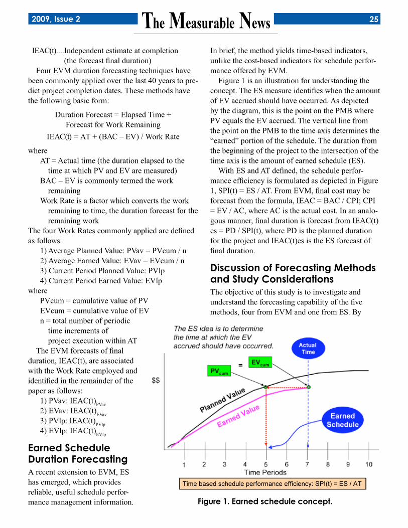
Figure 1 is an illustration for understanding the concept. The ES measure identifies when the amount of EV accrued should have occurred. As depicted by the diagram, this is the point on the PMB where PV equals the EV accrued. The vertical line from the point on the PMB to the time axis determines the “earned” portion of the schedule. The duration from the beginning of the project to the intersection of the time axis is the amount of earned schedule (ES).

With ES and AT defined, the schedule perfor-mance efficiency is formulated as depicted in Figure 1, SPI(t) = ES / AT. From EVM, final cost may be forecast from the formula, IEAC = BAC / CPI; CPI = EV / AC, where AC is the actual cost. In an analo-gous manner, final duration is forecast from IEAC(t)es = PD / SPI(t), where PD is the planned duration for the project and IEAC(t)es is the ES forecast of final duration.

Discussion of Forecasting Methods and Study ConsiderationsThe objective of this study is to investigate and understand the forecasting capability of the five methods, four from EVM and one from ES. By

Figure 1. Earned schedule concept.


website: www.CBTWorkshop.com phone: 888•644•5613

Let The CBT Workshop Assist You!

Staff Augmentation

Tools Implementation and Training

Skilled EVMS Planners, Schedulers, Program Control Analysts, Estimators, and EVMS Consultants

Short or Long Term Assignments Contract-to-hire personnel

We have EVMS tools experts who can implement, train, integrate, and migrate EVMS data in the following tools:

Microsoft Project and Project Server Deltek MPM, wInsight, Cobra, Open Plan Primavera

Everyone is Looking for Skilled EVMS Resources…We Have Them

EVMS Services

Web Based EVMS Training

EVMS Gap Analysis System Description Design and Development Desktop Operating Procedures IBR Preparation and Dispositioning CAM Training and Mock Interviews

EVMS Fundamentals and EVMS Advanced training, testing, and certification.

Call UsToday!

inspection, it can be deduced that the EVM Work Rates have mathematical failings that affect their performance.

When the project executes past its planned dura-tion, PVcum is equal to its maximum value, BAC, and is invariant thereafter. Thus the PVav Work Rate becomes PVav = BAC / m, where m is a number larger than the planned number of time periods for the project. Obviously as m becomes larger PVav is decreasingly smaller, thereby causing the work re-maining forecast to be longer than its planned time.

The situation for the PVlp Work Rate is more se-vere. After the planned project duration has passed, there are no periodic values of PV, thereby making the computation of IEAC(t)PVlp indeterminate. These observations are excluded from the study because it may be that IEAC(t)PVlp is a good predictor other-wise. A tenet of the study is to provide each method reasonable opportunity to show well, despite the known limitations.

The two Work Rates, EVav and EVlp, normally do not have indeterminate calculation conditions. There

is, however, one exception of when a period elapses with no EV accrued; this condition may occur for smaller projects that assess their status weekly. When EVlp is equal to zero, IEAC(t)EVlp cannot be calculated. Just as for PVlp, the condition is accommodated in the study so as to not discredit the overall forecasting performance of EVlp. When an anomalous instance is encountered, the forecast for the previous valid obser-vation is used.

The forecasting from ES does not experience inde-terminate calculation conditions. A common positive characteristic of all of the methods with the exception of IEAC(t)PVlp is they converge to the actual duration. The predictive capability of the four EVM-based meth-ods in this study may be superior to the two tested by Vanhoucke and Vandevoorde (2007, 2007–2008); those methods did not necessarily correctly calculate the ac-tual outcome duration at completion.

Study Hypothesis and MethodologyThe conjecture to be examined in the study is ES provides a better forecasting method of final proj-


ect duration than the four methods cited previously for EVM. To make a determination concerning this conjecture, the extreme case will be examined and tested. The test is constructed to show that the EVM methods as an aggregate produce better forecasts than does ES. If the EVM methods are shown to be superior to ES it will not be known which one of the EVM methods is better. Thus, if this is the deter-mination, further examination will be necessary to understand the circumstances for selecting the ap-propriate EVM forecasting method.

The hypothesis from the preceding discussion is formally defined as follows:

Ho: EVM methods produce the better forecast of final project duration

Ha: ES method produces the better forecast of final project duration

where Ho is the null hypothesis (i.e., the statement to be validated) and Ha is the alternate hypothesis (Wagner, 1992).

The statistical testing is performed using the Sign Test applied at 0.05 level of significance (National Institue of Standards and Technology Data Plot, 2005). Assuming each of the five methods has an equal probability of success, the probability for each trial is 0.8.

Data from 16 projects is used for generating the forecasts from each of the methods. These forecasts are then tested and analyzed. The test statistic for the hypothesis test is computed from the number of times the EVM methods are observed to yield the better forecast. Thus, for each testing condition applied the maximum number of successes for the EVM methods is 16. When the EVM methods suc-cesses are fewer than 10, the test statistic has a value in the critical region (< 0.05). A value in the critical region indicates there is enough evidence to reject the null hypothesis. In clearer language, this test result shows that the EVM methods do not produce duration forecasts better than those from ES. A test statistic value outside of the critical region is the converse, i.e., there is not enough evidence to reject the null hypothesis.

The test statistic is determined from the ranking of the standard deviations for each of the forecasting

methods for each project. The standard deviation is calculated from the differences between the forecast values computed at the project status points and the actual final duration as follows:

σm = [Σ (FVm(i) – FD)2 / (n-1)]0.5

whereσm = the standard deviation for forecasting method mFVm(i) = forecast value for method m at status

point (i)FD = actual final durationn = number of status pointsΣ = summation over a specific set of status points

The smallest value for the standard deviation in-dicates the best forecast produced. There are five forecasting methods, thus the ranking will be from 1 to 5; the rank of 1 is associated with the lowest value of standard deviation and 5 the highest. The ranking of the methods is performed for the 16 sets of proj-ect data. The number of times the rank of 1 occurs (without ties between the EVM methods) determines the test statistic value. By using the ranking approach, the unit for the periods (e.g., months, weeks) can be different between projects; the ranking of the five methods is performed separately for each project.

To understand whether a particular method is bet-ter for early, middle, late, or overall forecasting the projects are analyzed and tested for specific regions of performance. Seven groupings are formed us-ing the observations within various percent complete ranges to make the determinations: early (10% – 40%), middle (40% – 70%), late (70% – 100%), overall (10% – 100%). Additionally, other ranges are used to deter-mine if one of the methods converges to the actual final duration more rapidly than the others and thus is better for a portion of the forecast, but is not necessarily supe-rior overall. The ranges used for this purpose are: 25% – 100%, 50% – 100%, and 75% – 100%.

Data DiscussionA total of sixteen projects are included in the study. Twelve (1 through 12) are from one source with four (13 through 16) from a second. The output of the twelve projects is high-technology products. The remaining four projects are associated with informa-tion technology (IT) products.


The primary data requirement is that the proj-ects used in the study have not undergone any re-planning. The requirement is necessary to be able to discern the ability of the forecasting methods without having outside influence. All sixteen proj-

ects performed from beginning to completion with-out having baseline changes.Table 1 illustrates the schedule performance of the projects in the data set. The twelve high technology projects are measured in monthly periods whereas the four IT projects are

measured weekly. Two projects completed early, three on time and the remaining eleven deliv-ered later than planned.

Results AnalysisTo begin the analysis, it is in-structive to view the graphs from a single project (Project #13). The first graph, Figure 2, portrays the forecasting performance of all five methods along with the horizontal line for the actual fi-nal duration. It is observed that the prediction using the PVav and EVav Work Rates behave in a much less erratic manner than do the forecasts from the current period rates, PVlp and EVlp. The forecast from ES is seen to be much better than any of the EVM predictions, especially after the project completion point of 40%.

The next graph, Figure 3, por-trays similar information. It con-tains plots of the standard deviation versus percent complete for each of the EVM and ES methods. The behavior seen in Figure 2 is amplified by viewing the stan-dard deviation. As described for Figure 2, the average work rates are less volatile, while the current rates have large changes from one observation to the next. Again, the ES forecast is observed to be much more stable than any of the other methods. The standard deviation of the ES forecast is noticeably small-er than any of the other methods between 50 and 100% complete.

Table 1. Schedule performance.

Figure 2. Final duration forecasting comparisons (Project #13).

Figure 3. Standard Deviation Comparisons (Project 13).


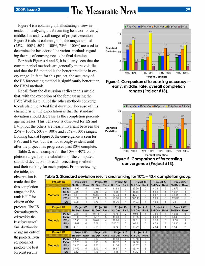
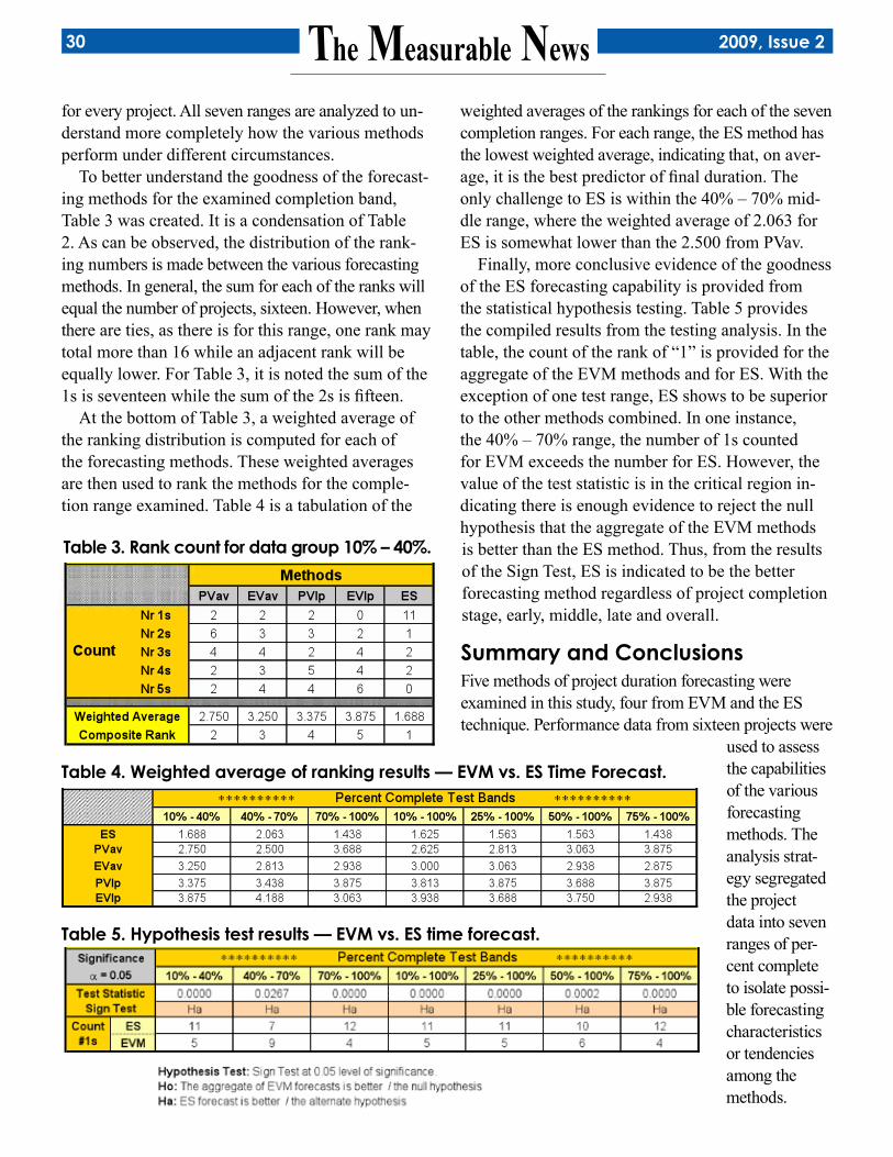
Figure 4 is a column graph illustrating a view in-tended for analyzing the forecasting behavior for early, middle, late and overall ranges of project execution. Figure 5 is also a column graph; the ranges applied (25% – 100%, 50% – 100%, 75% – 100%) are used to determine the behavior of the various methods regard-ing the rate of convergence to the final duration.

For both Figures 4 and 5, it is clearly seen that the current period methods are generally more volatile and that the ES method is the better predictor in ev-ery range. In fact, for this project, the accuracy of the ES forecasting method is significantly better than the EVM methods.

Recall from the discussion earlier in this article that, with the exception of the forecast using the PVlp Work Rate, all of the other methods converge to calculate the actual final duration. Because of this characteristic, the expectation is that the standard deviation should decrease as the completion percent-age increases. This behavior is observed for ES and EVlp, but the others are nearly invariant between the 25% – 100%, 50% – 100% and 75% – 100% ranges. Looking back at Figure 3, the convergence is seen for PVav and EVav, but it is not strongly evident until after the project has progressed past 80% complete.

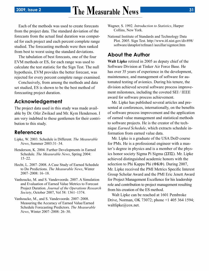
Table 2, is an example for the 10% – 40% com-pletion range. It is the tabulation of the computed standard deviations for each forecasting method and their ranking for each project. From reviewing the table, an observation is made that for this completion range, the ES rank is “1” for eleven of the projects. The ES forecasting meth-od provides the best forecasts of final duration for a large majority of the projects. Even so, it does not produce the best forecast results

Figure 4. Comparison of forecasting accuracy — early, middle, late, overall completion

ranges (Project #13).

Figure 5. Comparison of forecasting convergence (Project #13).

Table 2. Standard deviation results and ranking for 10% – 40% completion group.


for every project. All seven ranges are analyzed to un-derstand more completely how the various methods perform under different circumstances.

To better understand the goodness of the forecast-ing methods for the examined completion band, Table 3 was created. It is a condensation of Table 2. As can be observed, the distribution of the rank-ing numbers is made between the various forecasting methods. In general, the sum for each of the ranks will equal the number of projects, sixteen. However, when there are ties, as there is for this range, one rank may total more than 16 while an adjacent rank will be equally lower. For Table 3, it is noted the sum of the 1s is seventeen while the sum of the 2s is fifteen.

At the bottom of Table 3, a weighted average of the ranking distribution is computed for each of the forecasting methods. These weighted averages are then used to rank the methods for the comple-tion range examined. Table 4 is a tabulation of the

weighted averages of the rankings for each of the seven completion ranges. For each range, the ES method has the lowest weighted average, indicating that, on aver-age, it is the best predictor of final duration. The only challenge to ES is within the 40% – 70% mid-dle range, where the weighted average of 2.063 for ES is somewhat lower than the 2.500 from PVav.

Finally, more conclusive evidence of the goodness of the ES forecasting capability is provided from the statistical hypothesis testing. Table 5 provides the compiled results from the testing analysis. In the table, the count of the rank of “1” is provided for the aggregate of the EVM methods and for ES. With the exception of one test range, ES shows to be superior to the other methods combined. In one instance, the 40% – 70% range, the number of 1s counted for EVM exceeds the number for ES. However, the value of the test statistic is in the critical region in-dicating there is enough evidence to reject the null hypothesis that the aggregate of the EVM methods is better than the ES method. Thus, from the results of the Sign Test, ES is indicated to be the better forecasting method regardless of project completion stage, early, middle, late and overall.

Summary and ConclusionsFive methods of project duration forecasting were examined in this study, four from EVM and the ES technique. Performance data from sixteen projects were

used to assess the capabilities of the various forecasting methods. The analysis strat-egy segregated the project data into seven ranges of per-cent complete to isolate possi-ble forecasting characteristics or tendencies among the methods.

Table 3. Rank count for data group 10% – 40%.

Table 4. Weighted average of ranking results — EVM vs. ES Time Forecast.

Table 5. Hypothesis test results — EVM vs. ES time forecast.


Each of the methods was used to create forecasts from the project data. The standard deviation of the forecasts from the actual final duration was comput-ed for each project and each percent complete range studied. The forecasting methods were then ranked from best to worst using the standard deviations.

The tabulation of best forecasts, one of the four EVM methods or ES, for each range was used to calculate the test statistic for the Sign Test. The null hypothesis, EVM provides the better forecast, was rejected for every percent complete range examined.

Conclusively, from among the methods and data set studied, ES is shown to be the best method of forecasting project duration.

AcknowledgementThe project data used in this study was made avail-able by Dr. Ofer Zwikael and Mr. Kym Henderson. I am very indebted to these gentlemen for their contri-bution to this study.

ReferencesLipke, W. 2003. Schedule is Different. The Measurable

News, Summer 2003:31–34.

Henderson, K. 2004. Further Developments in Earned Schedule. The Measurable News, Spring 2004: 15–22.

Hecht, L. 2007–2008. A Case Study of Earned Schedule to Do Predictions. The Measurable News, Winter 2007–2008: 16–18.

Vanhoucke, M. and S. Vandevoorde. 2007. A Simulation and Evaluation of Earned Value Metrics to Forecast Project Duration. Journal of the Operations Research Society, October 2007, Vol 58: 1361–1374.

Vanhoucke, M., and S. Vandevoorde. 2007–2008. Measuring the Accuracy of Earned Value/Earned Schedule Forecasting Predictors. The Measurable News, Winter 2007–2008: 26–30.

Wagner, S. 1992. Introduction to Statistics, Harper Collins, New York.

National Institute of Standards and Technology Data Plot. 2005. Sign Test. http://www.itl.nist.gov/div898/software/dataplot/refman1/auxillar/signtest.htm

About the AuthorWalt Lipke retired in 2005 as deputy chief of the Software Division at Tinker Air Force Base. He has over 35 years of experience in the development, maintenance, and management of software for au-tomated testing of avionics. During his tenure, the division achieved several software process improve-ment milestones, including the coveted SEI / IEEE award for software process achievement.

Mr. Lipke has published several articles and pre-sented at conferences, internationally, on the benefits of software process improvement and the application of earned value management and statistical methods to software projects. He is the creator of the tech-nique Earned Schedule, which extracts schedule in-formation from earned value data.

Mr. Lipke is a graduate of the USA DoD course for PMs. He is a professional engineer with a mas-ter’s degree in physics and is a member of the phys-ics honor society Sigma Pi Sigma (ΣΠΣ). Mr. Lipke achieved distinguished academic honors with the selection to Phi Kappa Phi (ΦΚΦ). During 2007, Mr. Lipke received the PMI Metrics Specific Interest Group Scholar Award and the PMI Eric Jenett Award for Project Management Excellence for his leadership role and contribution to project management resulting from his creation of the ES method.

Walt Lipke can be reached at 1601 Pembroke Drive, Norman, OK 73072; phone +1 405 364 1594; [email protected].

Project Duration Forecasting … A Comparison of …earnedschedule.com/Docs/Project Duration...

Documents

Transcript of Project Duration Forecasting … A Comparison of …earnedschedule.com/Docs/Project Duration...