Progress Report for Thesis Research - …zadorlab.cshl.edu/asari/thesis/TCM06apr-hiro.pdfProgress...
14
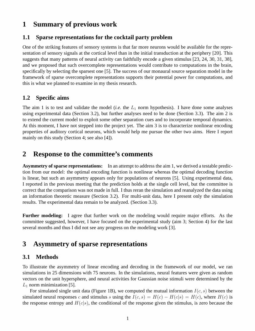
Progress Report for Thesis Research Sparse overcomplete representations as a principle for computation in the brain Hiroki Asari [email protected] April 20, 2006 Thesis committee members Carlos D. Brody (Chair) Alexei A. Koulakov Eero P. Simoncelli (NYU) Z. Josh Huang (academic mentor) Anthony M. Zador (research mentor)
Transcript of Progress Report for Thesis Research - …zadorlab.cshl.edu/asari/thesis/TCM06apr-hiro.pdfProgress...
Progress Report for Thesis Research
Sparse overcomplete representationsas a principle for computation in the brain
Hiroki Asari
April 20, 2006
Thesis committee members
Carlos D. Brody (Chair)Alexei A. KoulakovEero P. Simoncelli (NYU)Z. Josh Huang (academic mentor)Anthony M. Zador (research mentor)
1 Summary of previous work
1.1 Sparse representations for the cocktail party problem
One of the striking features of sensory systems is that far more neurons would be available for the repre-sentation of sensory signals at the cortical level than in the initial transduction at the periphery [20]. Thissuggests that many patterns of neural activity can faithfully encode a given stimulus [23, 24, 30, 31, 38],and we proposed that such overcomplete representations would contribute to computations in the brain,specifically by selecting the sparsest one [5]. The success of our monaural source separation model in theframework of sparse overcomplete representations supports their potential power for computations, andthis is what we planned to examine in my thesis research.
1.2 Specific aims
The aim 1 is to test and validate the model (i.e. the L1 norm hypothesis). I have done some analysesusing experimental data (Section 3.2), but further analyses need to be done (Section 3.3). The aim 2 isto extend the current model to exploit some other separation cues and to incorporate temporal dynamics.At this moment, I have not stepped into the project yet. The aim 3 is to characterize nonlinear encodingproperties of auditory cortical neurons, which would help me pursue the other two aims. Here I reportmainly on this study (Section 4; see also [4]).
2 Response to the committee’s comments
Asymmetry of sparse representations: In an attempt to address the aim 1, we derived a testable predic-tion from our model: the optimal encoding function is nonlinear whereas the optimal decoding functionis linear, but such an asymmetry appears only for populations of neurons [5]. Using experimental data,I reported in the previous meeting that the prediction holds at the single cell level, but the committee iscorrect that the comparison was not made in full. I thus reran the simulation and reanalyzed the data usingan information theoretic measure (Section 3.2). For multi-unit data, here I present only the simulationresults. The experimental data remain to be analyzed. (Section 3.3).
Further modeling: I agree that further work on the modeling would require major efforts. As thecommittee suggested, however, I have focused on the experimental study (aim 3; Section 4) for the lastseveral months and thus I did not see any progress on the modeling work [3].
3 Asymmetry of sparse representations
3.1 Methods
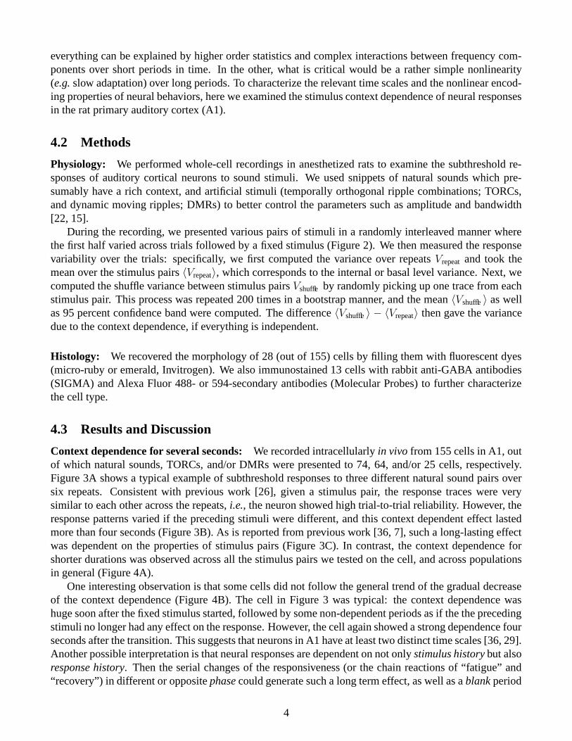
To illustrate the asymmetry of linear encoding and decoding in the framework of our model, we ransimulations in 25 dimensions with 75 neurons. In the simulations, neural features were given as randomvectors on the unit hypersphere, and neural activities for Gaussian noise stimuli were determined by theL1 norm minimization [5].
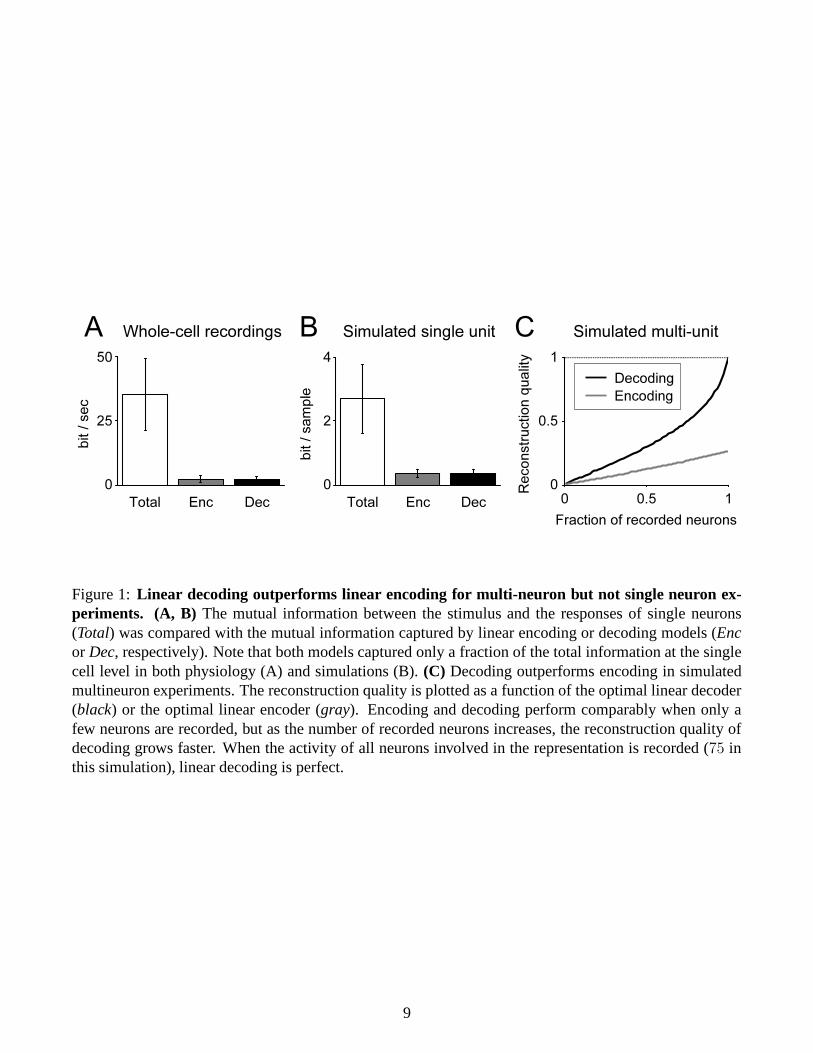
For simulated single unit data (Figure 1B), we computed the mutual information I(c, s) between thesimulated neural responses c and stimulus s using the I(c, s) = H(c) − H(c|s) = H(c), where H(c) isthe response entropy and H(c|s), the conditional of the response given the stimulus, is zero because the
1

relation between stimuli and responses was deterministic. Thus the mutual information between the singleneuron and the stimulus was just equal to the response entropy, which we estimated by direct binning fromthe histogram of neural responses (total information). We compared this information to either I(c, c) orI(s, s), the mutual information captured by linear encoding or decoding models, respectively, where the“hat” indicates the linear estimates. We used the Gaussian approximation for these information estimations[33].
For simulated multi-unit data (Figure 1C), the computation of the full mutual information was compu-tationally intractable. We therefore measured the following reconstruction quality of the models:
1 −
⟨
‖reconstruction error‖2
‖response or signal‖2
⟩
= 1 −
⟨
1
SNR
⟩
,
where ‖·‖2 denotes the L2 (Euclidean) norm and 〈·〉 the mean over data. Note that the measure is basedon the relative length (standard deviation) of the model errors, and that it gives zero for pure noise and onefor perfect reconstruction.
For experimental data (Figure 1A), a subset of data in the previous work was analyzed [26]. Specif-ically, we used whole-cell recording data for primary auditory cortical (A1) neurons in anesthetized ratsresponding to natural sounds. In a first data set (7 cells), a fixed subset of natural sounds were repeatedlypresented up to 20 times. These data were used to estimate total information using the direct method [8].In a second data set (8 cells), as many natural sounds as possible were tested, each once or twice. Both thefirst and the second sets of data were used to examine the performance of linear encoding and decodingmodels, in a similar manner to the analyses of simulated single unit data.
3.2 Results
Sparse overcomplete representations predict that linear models fail in both decoding and encoding direc-tions at the single cell level (Figure 1B), whereas decoding outperforms encoding at the multiple cell level(Figure 1C). Consistent with the first half of the prediction, neither linear encoding nor linear decodingworked at the single cell level for the rat auditory system (Figure 1A). I am now planning to test the secondhalf of the prediction under the assumption that multiple single-unit recordings from multiple animals canbe considered as equivalent as multi-unit recordings from single animals (Section 3.3).
3.3 Future directions
Linear models for populations of neurons: The regression methods to estimate linear filters can beeasily extended from single neurons to populations of neurons. As for physiological data, however, itwould be difficult to record simultaneous activities of multiple neurons in vivo (but see below). I wouldthus assume that neural responses to a given stimulus are deterministic in general, and that single-unitrecordings from multiple animals can be considered as equivalent as multi-unit recordings from singleanimals. Thus far, I have recorded from more than a hundred of neurons (Section 4), out of which a fixedset of natural sound stimuli was used for 48 neurons. This is by far less than the number of neurons in theauditory cortex, but I will use these data to examine if the asymmetry appears for populations of neurons. Itwould also be interesting to examine the difference, if any, between the subthreshold (membrane potential)and suprathreshold (spikes) responses.
Test sparseness: We claimed that sparse overcomplete representations would be very useful for com-putation in the brain. Based on the whole-cell recording data (Section 4), the spontaneous and evokedfiring rates in A1 were 0.35 ± 0.73 Hz and 0.37 ± 0.66 Hz (median ± interquartile range; n = 155),
2

respectively, and they were not significantly different (Wilcoxon matched-pairs signed-rank test). Thissuggests that most stimuli should elicit only modest firing in most neurons, indirectly supporting the ideaof sparse representations. But why not directly test the sparseness? With modern techniques (e.g. tetrodes,two-photon imaging, or molecular markers), it is not impossible to simultaneously record the activities ofmultiple neurons from single animals. However, I should think more because these techniques have prosand cons, and because such a project would require a huge investment of time and efforts.
Extended linear models: Up to now, linear filters were estimated in the sense of finite impulse re-sponses:
yt =
N∑
i=1
at−ixt−i, (1)
where xt−i and at−i are the input and the corresponding coefficient at time t−i, and yt is the linear estimateof the output at time t. Note the causality and that the performance of Eq.(1) can depend on the parameterN , the window length. To alleviate the dependence, we can extend Eq.(1) to infinite impulse responses,which is equivalent to introducing a feedback term:
yt =∞
∑
i=1
at−ixt−i ≈N
∑
i=1
a′
t−ixt−i +
M∑
i=1
bt−iyt−i. (2)
Furthermore, we can introduce an error correction term to make an adaptive model:
yt =
N∑
i=1
a′
t−ixt−i +
M∑
i=1
bt−iyt−i + et. (3)
The Eq.(3) can be implemented by a well-known method called the Kalman filters [19], which is optimalif all noise is Gaussian.
I will apply Eqs. (2)–(3) to the data set I have, and test if linear encoding models really fail to explainneural responses. I may also try the particle filters1 [2] or some other nonlinear and/or adaptive methods.For this type of regression analyses, however, a model should be chosen very carefully because the modelinterpretability as well as the fitness to data is very important. It would then be interesting to examinelinear-in-the-parameter models using local or radial basis functions [14, 17] since the L1 norm hypothesisimplies piecewise linear encoding functions [5].
4 Context dependence of auditory cortical neurons
4.1 Background and Motivation
How do past events influence auditory cortical responses? Psychophysical studies have demonstrated thatstimulus context strongly affects perception and auditory scene analysis in humans [9]. Physiologicalstudies on the effects of stimulus context (e.g. forward masking, background and foreground represen-tations) suggest that the responses of auditory cortical neurons are highly dependent on stimulus history[1, 18, 32, 6, 7, 10, 11, 37]. However, the responses cannot be fully explained by linear encoding (spectro-temporal receptive field; STRF) models despite their high trial-to-trial reliability [25, 26], and little isknown about the details of the underlying neuronal dynamics. In one extreme, we could imagine that
1A non-parametric model that can deal with non-Gaussian noise and nonlinearities.
3
everything can be explained by higher order statistics and complex interactions between frequency com-ponents over short periods in time. In the other, what is critical would be a rather simple nonlinearity(e.g. slow adaptation) over long periods. To characterize the relevant time scales and the nonlinear encod-ing properties of neural behaviors, here we examined the stimulus context dependence of neural responsesin the rat primary auditory cortex (A1).
4.2 Methods
Physiology: We performed whole-cell recordings in anesthetized rats to examine the subthreshold re-sponses of auditory cortical neurons to sound stimuli. We used snippets of natural sounds which pre-sumably have a rich context, and artificial stimuli (temporally orthogonal ripple combinations; TORCs,and dynamic moving ripples; DMRs) to better control the parameters such as amplitude and bandwidth[22, 15].
During the recording, we presented various pairs of stimuli in a randomly interleaved manner wherethe first half varied across trials followed by a fixed stimulus (Figure 2). We then measured the responsevariability over the trials: specifically, we first computed the variance over repeats Vrepeat and took themean over the stimulus pairs 〈Vrepeat〉, which corresponds to the internal or basal level variance. Next, wecomputed the shuffle variance between stimulus pairs Vshuffle by randomly picking up one trace from eachstimulus pair. This process was repeated 200 times in a bootstrap manner, and the mean 〈Vshuffle 〉 as wellas 95 percent confidence band were computed. The difference 〈Vshuffle 〉 − 〈Vrepeat〉 then gave the variancedue to the context dependence, if everything is independent.
Histology: We recovered the morphology of 28 (out of 155) cells by filling them with fluorescent dyes(micro-ruby or emerald, Invitrogen). We also immunostained 13 cells with rabbit anti-GABA antibodies(SIGMA) and Alexa Fluor 488- or 594-secondary antibodies (Molecular Probes) to further characterizethe cell type.
4.3 Results and Discussion
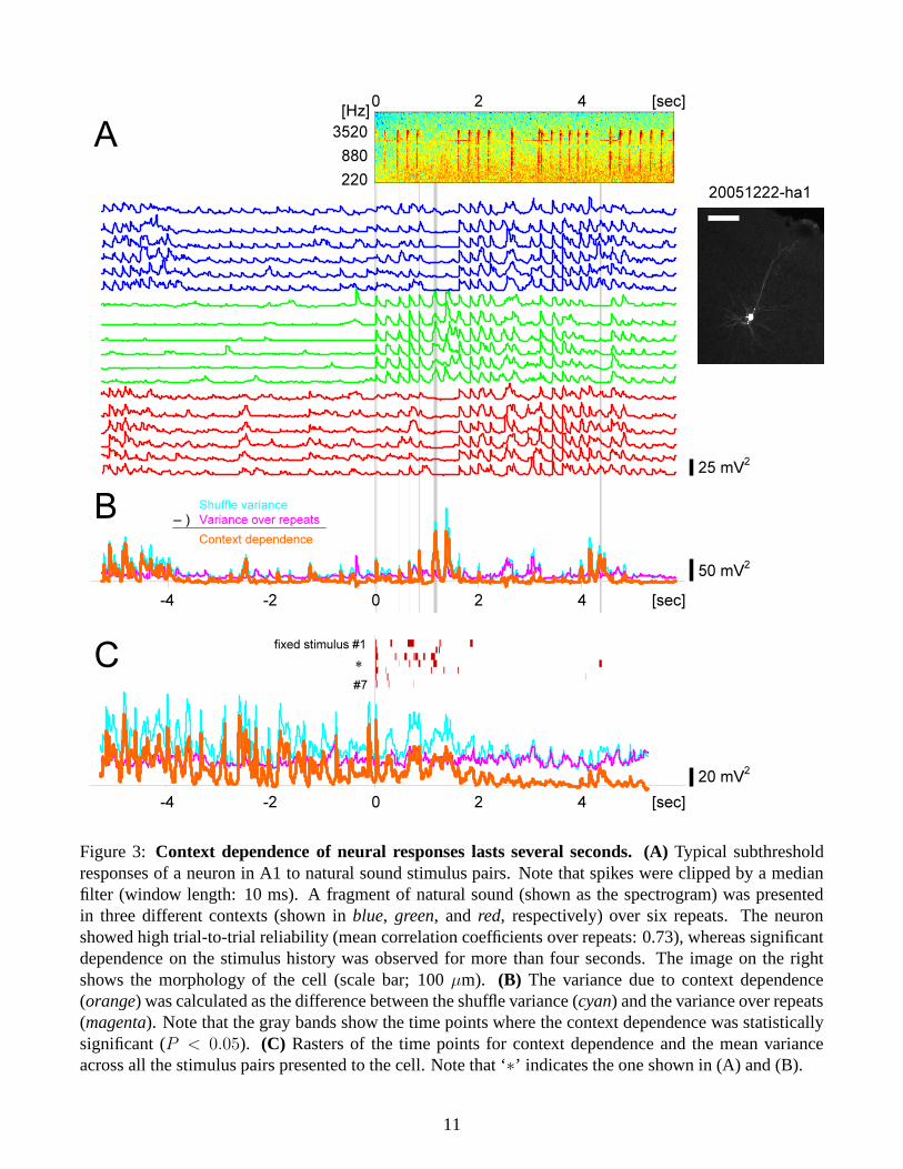
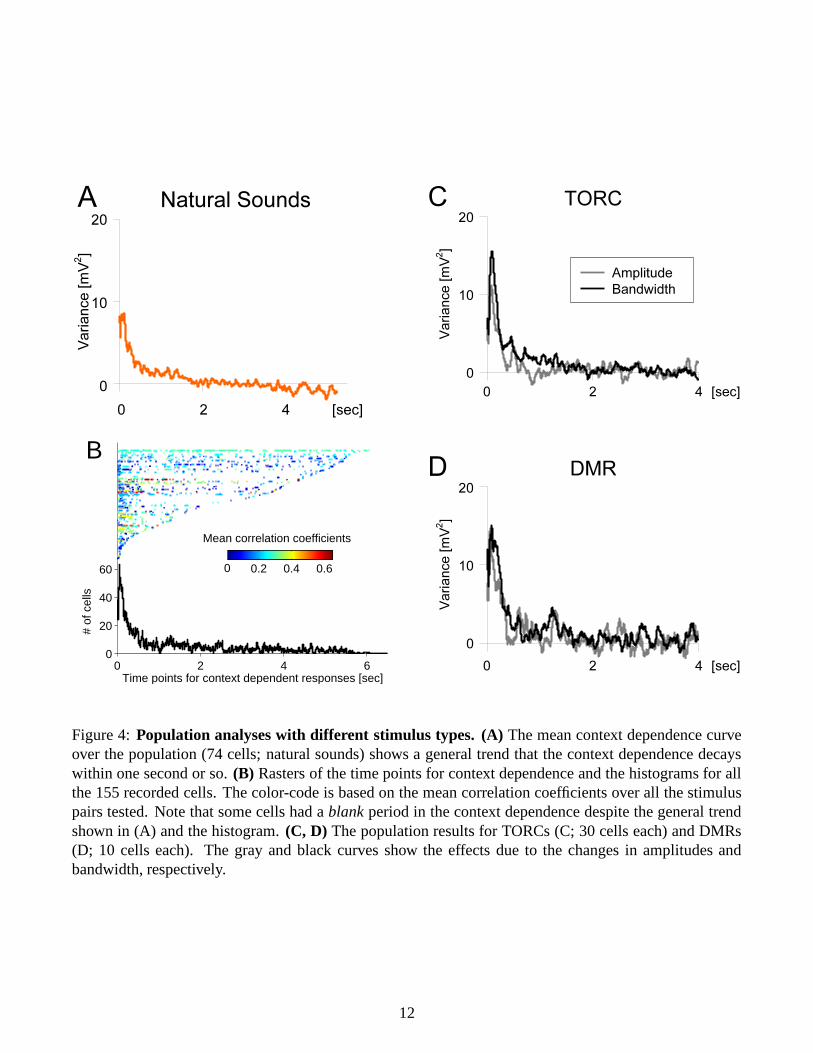
Context dependence for several seconds: We recorded intracellularly in vivo from 155 cells in A1, outof which natural sounds, TORCs, and/or DMRs were presented to 74, 64, and/or 25 cells, respectively.Figure 3A shows a typical example of subthreshold responses to three different natural sound pairs oversix repeats. Consistent with previous work [26], given a stimulus pair, the response traces were verysimilar to each other across the repeats, i.e., the neuron showed high trial-to-trial reliability. However, theresponse patterns varied if the preceding stimuli were different, and this context dependent effect lastedmore than four seconds (Figure 3B). As is reported from previous work [36, 7], such a long-lasting effectwas dependent on the properties of stimulus pairs (Figure 3C). In contrast, the context dependence forshorter durations was observed across all the stimulus pairs we tested on the cell, and across populationsin general (Figure 4A).
One interesting observation is that some cells did not follow the general trend of the gradual decreaseof the context dependence (Figure 4B). The cell in Figure 3 was typical: the context dependence washuge soon after the fixed stimulus started, followed by some non-dependent periods as if the the precedingstimuli no longer had any effect on the response. However, the cell again showed a strong dependence fourseconds after the transition. This suggests that neurons in A1 have at least two distinct time scales [36, 29].Another possible interpretation is that neural responses are dependent on not only stimulus history but alsoresponse history. Then the serial changes of the responsiveness (or the chain reactions of “fatigue” and“recovery”) in different or opposite phase could generate such a long term effect, as well as a blank period
4

in the context dependence simply due to the coincidence of the transition periods between responsive andnon-responsive states.
No difference between amplitude and bandwidth effects: We then used artificial stimuli to study whatstimulus factors contribute to the context dependence. In one case we systematically changed amplitudes(over 30 dB attenuations) of the preceding stimuli with a fixed bandwidth, whereas in the other we variedbandwidth (within the range of 8 octaves) with a fixed amplitude. However, we did not see any differencein the context dependence curves (Figures 4C and 4D), and it is not clear yet what is critical to determinethe neural behaviors. We also examined the relation between the longest context dependence observed andthe cortical layers (or the depth from the surface), but there was no apparent correlation (data not shown).
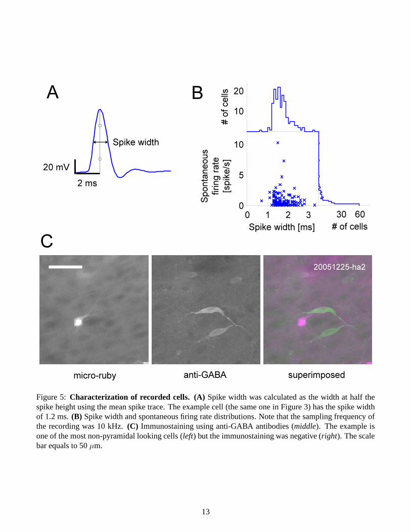
Characterization of recorded cells: To further analyze the data, we tried to characterize the cell types,specifically to identify whether the cells were inhibitory or excitatory. We first looked at spike width andfiring rates, but the distributions were unimodal (Figure 5B) and we did not find any “thin- or fast-spiking”cell [28, 34], which is a characteristic of a subclass of interneurons [12, 16, 27]. We then performedimmunostaining using anti-GABA antibodies, but none of the cells we tested was positive (Figure 5C).Note that it could be false-negative since the sections were thick2 (100 µm) and thus the antibodies couldnot reach the middle of the sections. But these results raise the possibility that we recorded mostly frompyramidal (or “principal”) cells in A1 in somewhat biased manner.
4.4 Future directions
I will record some more neurons in A1 and characterize the cell types by the immunostaining. This isworth doing (1) to remove the concern for the false-negative (Section 4.3), and (2) to collect more datafor the population analyses (Section 3.3). In the meantime, I will look deeply at the data and think aboutbetter analysis methods. For example, I mentioned in Section 4.3 that some cells had a blank period in thecontext dependence (Figure 4B). However, the current analysis method does not tell whether this is true3
or simply because cells did not respond well to the input stimuli during the period. A better quantitativemeasure will be required to address this question.
It is also interesting to think about the mechanisms. The existence of multiple time scales suggeststhat the stimulus history might be stored not only in the cells but also somewhere in the network. Thiscould be examined by pharmacology, or by recording different brain areas (e.g. thalamus). We could alsosimultaneously record the nearby local field potential (LFP) to test the relation to the “cortical state” [13].However, I would rather take computational approaches to study the underlying mechanisms in details(Section 3.3): e.g. the feedback and error correction terms in shorter and longer time scales, respectively, inEq.(3). Also note that a′ and b in Eqs. (2)–(3) correspond to the stimulus- and response-history dependenteffects, respectively.
2Slices are often much thinner for the immunocytochemistry; e.g. 60 µm in [21], 40 µm in [35].3I believe this is true at least for the typical cell shown in Figure 3.
5
References
[1] Abeles, M. and Goldstein, M. H. (1972). Responses of single units in the primary auditory cortex ofthe cat to tones and to tone pairs. Brain Res 42(2): 337–352.
[2] Arulampalam, S., Maskell, S. R., Gordon, N. J., and Clapp, T. (2002). A tutorial on particle filtersfor online nonlinear/non-gaussian bayesian tracking. IEEE Transactions on Signal Processing 50:174–188.
[3] Asari, H. (2005). Estimation of the optimal neural features in the context of sparse overcompleterepresentations. (http://zadorlab.cshl.edu/asari/pdf/BasisEst.pdf).
[4] Asari, H., Oviedo, H., and Zador, A. M. (2006). Context dependence of neural responsesin rat primary auditory cortex. Poster, Computational and Systems Neuroscience meeting(http://zadorlab.cshl.edu/asari/pdf/cosyne2006p.pdf).
[5] Asari, H., Pearlmutter, B. A., and Zador, A. M. (2006). Sparse representations for the cocktail partyproblem. Submitted (http://zadorlab.cshl.edu/asari/pdf/hrtfsource.pdf).
[6] Bar-Yosef, O., Rotman, Y., and Nelken, I. (2002). Responses of neurons in cat primary auditorycortex to bird chirps: effects of temporal and spectral context. J Neurosci 22(19): 8619–32.
[7] Bartlett, E. L. and Wang, X. (2005). Long-lasting modulation by stimulus context in primate auditorycortex. J Neurophysiol 94(1): 83–104.
[8] Borst, A. and Theunissen, F. E. (1999). Information theory and neural coding. Nat Neurosci. 2(11):947–957.
[9] Bregman, A. S. (1990). Auditory Scene Analysis: The Perceptual Organization of Sound. MIT Press,Cambridge, Massachusetts.
[10] Brosch, M. and Schreiner, C. (1997). Time course of forward masking tuning curves in cat primaryauditory cortex. J Neurophysiol 77(2): 923–43.
[11] Brosch, M. and Schreiner, C. (2000). Sequence sensitivity of neurons in cat primary auditory cortex.Cereb Cortex 10(12): 1155–67.
[12] Connors, B. W. and Gutnick, M. J. (1990). Intrinsic firing patterns of diverse neocortical neurons.Trends Neurosci 13(3): 99–104.
[13] Deweese, M. R. and Zador, A. M. (2004). Shared and private variability in the auditory cortex. JNeurophysiol 92(3): 1840–1855.
[14] Duda, R., Hart, P., and Stork, D. (2001). Pattern Classification (2nd ed.). Wiley Interscience.
[15] Escabi, M. A. and Schreiner, C. E. (2002). Nonlinear spectrotemporal sound analysis by neurons inthe auditory midbrain. J Neurosci 22(10): 4114–4131.
[16] Freund, T. F. and Buzsaki, G. (1996). Interneurons of the hippocampus. Hippocampus 6(4): 347–470.
[17] Hastie, T., Tibshirani, R., and Friedman, J. (2001). The elements of statistical learning theory.Springer, New York.
6
[18] Hocherman, S. and Gilat, E. (1981). Dependence of auditory cortex evoked unit activity on inter-stimulus interval in the cat. J Neurophysiol 45(6): 987–997.
[19] Kalman, R. E. (1960). A new approach to linear filtering and prediction problems. Transactions ofthe ASME–Journal of Basic Engineering 82(Series D): 35–45.
[20] Kandel, E. R., Schwartz, J. H., and Jessel, T. M. (2000). Principles of Neural Science, 4th ed.McGraw-Hill.
[21] Klausberger, T., Magill, P. J., Marton, L. F., Roberts, J. D. B., Cobden, P. M., Buzsaki, G., andSomogyi, P. (2003). Brain-state- and cell-type-specific firing of hippocampal interneurons in vivo.Nature 421: 844–848.
[22] Klein, D. J., Depireux, D. A., Simon, J. Z., and Shamma, S. A. (2000). Robust spectrotemporalreverse correlation for the auditory system: optimizing stimulus design. J Comput Neurosci 9(1):85–111.
[23] Lee, T. W., Lewicki, M. S., and Sejnowski, T. J. (2000). ICA mixture models for unsupervisedclassification of non-gaussian classes and automatic context switching in blind signal separation.IEEE Transactions on Pattern Analysis and Machine Intelligence 22(10): 1078–1089.
[24] Lewicki, M. S. and Sejnowski, T. J. (2000). Learning overcomplete representations. Neural Comput.12(2): 337–365.
[25] Linden, J. F., Liu, R. C., Sahani, M., Schreiner, C. E., and Merzenich, M. M. (2003). Spectrotemporalstructure of receptive fields in areas AI and AAF of mouse auditory cortex. J. Neurophysiol. 90(4):2660–2675.
[26] Machens, C. K., Wehr, M. S., and Zador, A. M. (2004). Linearity of cortical receptive fields measuredwith natural sounds. J. Neurosci. 24(5): 1089–1100.
[27] McBain, C. J. and Fisahn, A. (2001). Interneurons unbound. Nat Rev Neurosci 2(1): 11–23.
[28] Mountcastle, V. B., Talbot, W. H., Sakata, H., and Hyvarinen, J. (1969). Cortical neuronal mech-anisms in flutter-vibration studied in unanesthetized monkeys. Neuronal periodicity and frequencydiscrimination. J Neurophysiol 32(3): 452–484.
[29] Nelken, I. (2004). Processing of complex stimuli and natural scenes in the auditory cortex. Curr OpinNeurobiol 14(4): 474–480.
[30] Olshausen, B. A. and Field, D. J. (1996). Emergence of simple-cell receptive field properties bylearning a sparse code for natural images. Nature 381: 607–609.
[31] Olshausen, B. A. and Field, D. J. (1997). Sparse coding with an overcomplete basis set: A strategyemployed by V1?. Vision Research 37(23): 3311–3325.
[32] Phillips, D. P. (1985). Temporal response features of cat auditory cortex neurons contributing tosensitivity to tones delivered in the presence of continuous noise. Hear Res 19(3): 253–268.
[33] Rieke, F., Warland, D., de Ruyter van Steveninck, R., and Bialek, W. (1997). Spikes: Exploring theNeural Code. MIT Press, Cambridge, Massachusetts.
7

[34] Simons, D. J. (1978). Response properties of vibrissa units in rat SI somatosensory neocortex. JNeurophysiol 41(3): 798–820.
[35] Tseng, K. Y., Mallet, N., Toreson, K. L., Moine, C. L., Gonon, F., and O’donnell, P. (2006). Excita-tory response of prefrontal cortical fast-spiking interneurons to ventral tegmental area stimulation invivo.. Synapse 59(7): 412–417.
[36] Ulanovsky, N., Las, L., Farkas, D., and Nelken, I. (2004). Multiple time scales of adaptation inauditory cortex neurons. J Neurosci 24(46): 10440–53.
[37] Wehr, M. and Zador, A. M. (2005). Synaptic mechanisms of forward suppression in rat auditorycortex. Neuron 47(3): 437–45.
[38] Zibulevsky, M. and Pearlmutter, B. A. (2001). Blind source separation by sparse decomposition in asignal dictionary. Neural Comput. 13(4): 863–882.
8
B1
0. 5
0Reco
nstru
ction
quali
ty
CSimulated single unit
0 0. 5 1
E ncodingD ecoding
T otal E nc D ec
4
2
0
bit / s
ample
Simulated multi-unit
Fraction of recorded neurons
A
T otal E nc D ec
5 0
25
0
bit / s
ec
W h o le-c ell r ec o r dings
Figure 1: Linear decoding outperforms linear encoding for multi-neuron but not single neuron ex-periments. (A, B) The mutual information between the stimulus and the responses of single neurons(Total) was compared with the mutual information captured by linear encoding or decoding models (Encor Dec, respectively). Note that both models captured only a fraction of the total information at the singlecell level in both physiology (A) and simulations (B). (C) Decoding outperforms encoding in simulatedmultineuron experiments. The reconstruction quality is plotted as a function of the optimal linear decoder(black) or the optimal linear encoder (gray). Encoding and decoding perform comparably when only afew neurons are recorded, but as the number of recorded neurons increases, the reconstruction quality ofdecoding grows faster. When the activity of all neurons involved in the representation is recorded (75 inthis simulation), linear decoding is perfect.
9

Response v a r i a b i l i t y
T i m e
T r i a l sV a r i a b l e st i m u l i
Rel ev a nt t i m e sc a l e
F i x ed st i m u l i
Vshuffle VrepeatVshuffle Vrepeat
Figure 2: Experimental design to examine context dependence. In this example, various instrumentalsounds (flute, horn, and violin) are followed by a fixed piano melody. Neural responses to the piano melodycan be different depending on the preceding sounds, and the variability is measured as the differencebetween the shuffle variance 〈Vshuffle 〉 and the variance over repeats 〈Vrepeat〉, which is generally high in thefirst half and gradually decreases after the transition towards the basal level as the fixed stimulus continues.
10
A
B Shuffle varianceV ariance o ver rep eat s– )C o nt ex t d ep end ence
-4 -2 0 2 4 [ s e c ]
0 2 4 [ s e c ]3 5 208 8 0220
[ H z ]
5 0 m V 2
25 m V 2
2005 1222-ha1
fix ed s t im ulus # 1
# 7*C
20 m V 2
-4 -2 0 2 4 [ s e c ]
Figure 3: Context dependence of neural responses lasts several seconds. (A) Typical subthresholdresponses of a neuron in A1 to natural sound stimulus pairs. Note that spikes were clipped by a medianfilter (window length: 10 ms). A fragment of natural sound (shown as the spectrogram) was presentedin three different contexts (shown in blue, green, and red, respectively) over six repeats. The neuronshowed high trial-to-trial reliability (mean correlation coefficients over repeats: 0.73), whereas significantdependence on the stimulus history was observed for more than four seconds. The image on the rightshows the morphology of the cell (scale bar; 100 µm). (B) The variance due to context dependence(orange) was calculated as the difference between the shuffle variance (cyan) and the variance over repeats(magenta). Note that the gray bands show the time points where the context dependence was statisticallysignificant (P < 0.05). (C) Rasters of the time points for context dependence and the mean varianceacross all the stimulus pairs presented to the cell. Note that ‘∗’ indicates the one shown in (A) and (B).
11
0 2 4 [sec]
20
1 0
0
Natural SoundsA
Varia
nce [
mV2 ]
0 2 4 60
20
40
60
Time points for context dependent responses [sec]
# of
cel
ls
0.2 0.4 0.6
Mean correlation coefficients
0
B
AmplitudeB a n dw idth
0 2 4 [ s ec ]
TORC
2 0
1 0
0
D M RD
0 2 4 [ s ec ]
2 0
1 0
0
Varia
nce [
mV2 ]
Varia
nce [
mV2 ]
C
Figure 4: Population analyses with different stimulus types. (A) The mean context dependence curveover the population (74 cells; natural sounds) shows a general trend that the context dependence decayswithin one second or so. (B) Rasters of the time points for context dependence and the histograms for allthe 155 recorded cells. The color-code is based on the mean correlation coefficients over all the stimuluspairs tested. Note that some cells had a blank period in the context dependence despite the general trendshown in (A) and the histogram. (C, D) The population results for TORCs (C; 30 cells each) and DMRs(D; 10 cells each). The gray and black curves show the effects due to the changes in amplitudes andbandwidth, respectively.
12
2 ms
S p i k e w i d t h
20 mV
A
S p i k e w i d t h [ ms]0 1 2 3
Spon
taneo
us
firing
rate
[spike
/s]
1 0
5
0
B 201 0
# of c
ells
# of cells3 0 6 0
C
mi cr o-r u b y a n t i -G A B A su p er i mp osed
20051225-ha2
Figure 5: Characterization of recorded cells. (A) Spike width was calculated as the width at half thespike height using the mean spike trace. The example cell (the same one in Figure 3) has the spike widthof 1.2 ms. (B) Spike width and spontaneous firing rate distributions. Note that the sampling frequency ofthe recording was 10 kHz. (C) Immunostaining using anti-GABA antibodies (middle). The example isone of the most non-pyramidal looking cells (left) but the immunostaining was negative (right). The scalebar equals to 50 µm.
13