Program for two-dimensional interpretation of data ...

1

Zond geophysical software

Saint-Petersburg 2001-2016

Program for two-dimensional interpretation of data

obtained by magnetotelluric sounding

(МТ, АМТ, RМТ)

ZONDMT2D

Program functionality ........................................................................................................ 3

System requirements ........................................................................................................... 5

Program installation and deinstallation ............................................................................ 5

Program registration .......................................................................................................... 5

Adopted definitions ............................................................................................................. 5

Starting working and basic options .................................................................................... 6

Working guidelines ..................................................................................................................... 6

Creation and opening of data file .............................................................................................. 7

Main Window Toolbar ............................................................................................................... 9

Main Menu Functions ................................................................................................................ 9

“Hot” keys ................................................................................................................................. 15

Status bar .................................................................................................................................. 15

Adjusting starting model mesh settings .................................................................................. 15

Main data file format ........................................................................................................ 18

Preparing data for inversion ............................................................................................ 19

Options for data measurements editing .................................................................................. 19

Module of quality control and data editing ............................................................................ 24

Static shift correction ............................................................................................................... 29

Apparent parameters visualization .................................................................................. 31

Graphics plot ............................................................................................................................. 31

Pseudosection ............................................................................................................................ 33

Input and editing topographic information ..................................................................... 34

Data inversion ................................................................................................................... 36

Calibration of model mesh and operations with relief .......................................................... 36

Program parameters setup dialog ........................................................................................... 36

Inversion in layered medium ................................................................................................... 43

Incorporating a priori information in the inversion ............................................................. 45

2



Set boundaries dialog ............................................................................................................... 46

Model visualization modes and parameters ..................................................................... 47

Interpretation results saving ............................................................................................ 50

Modeling and working with model .................................................................................. 51

Survey layout definition ........................................................................................................... 51

Model building in ZondMT2D ................................................................................................ 52

Model editor .............................................................................................................................. 52

Working with block model ....................................................................................................... 52

Cell summarization dialog ....................................................................................................... 55

Polygonal modeling .................................................................................................................. 57

Working with multiple model in a single project ............................................................. 60

Data import and export ..................................................................................................... 62

Additional information visualization ...................................................................................... 62

Text (tabular) data files – import and export ........................................................................ 66

Exporting image setup dialog .................................................................................................. 66

Borehole columns and logging data visualization .................................................................. 67

Window of geological-geophysical model builder ........................................................... 72

Geoelectric models volumetric visualization using several profiles ............................... 73

Appendix 1: Graphics editor ............................................................................................ 77

Appendix 2: Graphics set editor ....................................................................................... 79

Appendix 3: Graphic’s legend editor ............................................................................... 80

Appendix 4: Pseudosection (contour section) parameters setup dialog ......................... 81

Appendix 5: Axes editor ................................................................................................... 83

Appendix 6: Dialog of Model visualization parameters .................................................. 86

Appendix 7: Pseudosection points editor ......................................................................... 88

Appendix 8. Zdconvert program ...................................................................................... 88

3



Program functionality

«ZONDMT2D» is computer program for 2D interpretation of profile data obtained by

magnetotelluric sounding. Friendly interface and ample opportunities for data presentation

allows solving assigned problem with maximum efficiency.

Basic feature of magnetotelluric field in two-dimensionally heterogeneous medium is its

division into two independent parts called polarizations or modes. The main difference between

E-polarized and H-polarized fields consists in the fact that in the former anomalies have

inductive origin while in the latter - galvanic. In case of E-polarization, electric field is polarized

along structures and for this reason it does not cross boundaries of areas with different resistivity.

Anomalies are caused by excess currents induced in conductive heterogeneities or by low

number of excess currents induced in nonconducting heterogeneities. In case of H-polarization,

currents flow transversely to structures. Thereby they cross boundaries of heterogeneities and

anomalies are caused by galvanic current flow inside them (for low-resistivity heterogeneities) or

around them (for high-resistivity heterogeneities).

Problem of studying 2D fields comes to separate consideration of two tasks: for E-

polarization and for H-polarization. Solution of these tasks is much easier than Maxwell

equations system solution.

Maxwell equations for electric polarization Te are given below:

y

1

i

Exy

z

1

i

Exz

Ex (1)

where - field oscillation circular frequency, 0 - permeability of free space.

In this case medium in point neighborhood is supposed to be homogeneous with

electrical conductance . Solution of this equation gives Ex distribution in modeling area. Two

components of magnetic field can be found using Ex:

Hy 1

i

Exz

Hz 1

i

Exy (2)

Apparent resistivity and phase for Ex and Hy are calculated using the following formulas:

xy 1

i

ExHy

2

xy argEx

Hy

(3)

In case of magnetic polarization Tm Maxwell equation has the following form.

4



y

1

Hxy

z

1

Hxz

iH x

. (4)

Solution of this equation gives Ex distribution in modeling area. Two components of

electric field can be found using Hx:

Ey 1

Hxz

Ez 1

Hxy . (5)

Apparent resistivity and phase for magnetic polarization can be calculated in the same

way.

Finite-element method as mathematical apparatus is used to solve forward and inverse

problems. It gives best results in comparison with mesh methods.

For plane-wave electromagnetic field modeling medium is divided into triangle cells grid

with different resistivity. Field behavior inside grid cell is approximated by linear basis function.

A

czbxazxN

2),(

(6)

Least squares method with regularization is used for inverse problem solution

(inversion). Regularization increases solution stability and allows receiving smoother resistivity

distribution.

RCmCfWAmRCCWAWA TTTTTT (7)

where A – the Jacobian matrix of partial derivatives, C – smoothing operator, W – relative

error matrix, m – section parameters vector, μ - regularizing parameter, Δf – discrepancy vector

between observed and calculated values, R – focusing operator.

During inverse problem solution development special attention was devoted to a priori

information accounting (data weights, parameters turndown).

«ZONDMT2D» has powerful system of profile data visualization, data editor, and system

of sensitivity and method resolution analysis.

Two types of graphics are used to display observed and calculated data, their discrepancy

or measurement weights in the program. They are graphics plan and pseudosection.

User can find measurements’ parameters, set data weights (relevance) and correct

measured values in data editor. It is possible to set data weights in accordance with noise level

and by total sensitivity of current measurement to medium parameters or fix those cells of the

model which have parameters that almost do not influence measuring results.

In resolution analysis system user can study model sensitivity function that is level of cell

influence on measuring result.

5



)( AAdiagS T (8)

Research of sensitivity allows choosing optimal selection of frequencies and

measurement interval in order to solve assigned geologic task.

«ZONDMT2D» uses simple and clear data file format. Apparent resistivity and phase for

two types of polarization can be used as measured characteristics. Program allows importing and

visualizing data using other methods which makes data interpretation process more integrated.

«ZONDMT2D» has modeling system that allows user to specify frequency set and

positions of measuring points.

«ZONDMTD» is easy-to-use instrument for automatic and interactive interpretation of

profile magnetotelluric sounding data and can be used on IBM-PC compatible PC with Windows

system.

System requirements

«ZONDMT2D» can be installed on PC with OS Windows 98 and higher. Recommended

system parameters are processor P IV-2 GHz, memory 512 Mb, screen resolution 1024 X 768,

color mode – True color (screen resolution change is not recommended while working with

data).

Program installation and deinstallation

«ZONDMT2D» program is supplied on CD or by internet. Current manual is included in

the delivery set. Latest updates of the program can be downloaded from website: www.zond-

geo.ru.

To install the program copy it from CD to necessary directory (e.g., Zond). To install

updates rewrite previous version of the program with the new one.

Secure key SenseLock driver must be installed before starting the program. To do that

open SenseLock folder (the driver can be downloaded from CD or website) and run

InstWiz3.exe file. After installation of the driver insert key. If everything is all right, a message

announcing that the key is detected will appear in the lower system panel.

To uninstall the program delete work directory of the program.

Program registration

For registration click “Registration file” item of the main menu of the program. When a

dialog appears, select registration file name, and save it. Created file is transmitted to specified in

the contract address. After that user receives unique password which depends on HDD serial

number. Input this password in “Registration” field. The second option is to use the program

with supplied SenseLock key inserted in USB-port while working.

Adopted definitions

Ro_a – apparent resistivity, Om*m.

6



Phi - impedance phase, degrees. Positive number. Should be specified in quadrant from 0

to 90 degrees.

Frequency in Hz.

Period is inverse value of measurement frequency, seconds.

Pseudodepth – approximate depth of investigation connected with scin-layer thickness.

All geometric values are specified in kilometers.

Starting working and basic options

Working guidelines

This section briefly describes how to work with the program «ZONDMT2D». To get

started after the first program run it is necessary to register the program by one of the methods

specified in Program registration: using a registration file, or the key SenseLock.

To take a geoelectric section (inversion mode), open the data file in the main menu

File/Open file.

To create a data file is recommended to use a helper program Zdconvert (more details in

Appendix 8). The program also supports REBOCC file format and EDI data format (more details

in «Opening REBOCC and EDI data files format»).

After opening a data file, starting model settings dialog window will appear (Mesh

constructor). Mesh parameters of the resulting geoelectric model are determined in the dialog

window. This dialog is described in details in «Adjusting starting model mesh settings». Usually

default settings can be used. After configuring the mesh press Apply button, and the program

goes on to working mode.

The program main window consists of three parts. The upper - is section or graphics of

measured parameters, the middle – section or graphs of calculated parameters. The bottom - a

model environment.

The next step is data processing and editing, including filtering, coordinate system

rotation, input correction to compensate for static shift etc. This option is implemented by the

tool Options/MT Editor and is described in «Module of quality control and data editing».

Before starting inversion it is necessary to set inversion parameters, using dialog Program

Setup. It is available in the Main Menu Options/Program setup or using the button on the

toolbar. More information about setting inversion parameters in the "Program parameters setup

dialog".

To start the inversion it is necessary to press the button on the toolbar. After the

calculation, it is possible to estimate values of relative discrepancy on the program status bar. It

is also possible to visually compare observed and calculated data using dialog of viewing

sounding curves (more in «Sounding curves view and edit dialog»), and displaying data as

Pseudosection or Graphics.

After obtaining the model (the lower section of the program main window) it is necessary

to save the calculation results in a ZondMT2D project format and/or one of the proposed

graphical and tabular formats (more details in «Interpretation results saving»).

If the work is being carried out in the modeling mode, it is not necessary to load the data

file, but create a synthetic observation system with any parameters, specify medium geometry

7



and properties. After calculating the forward problem, results can be saved. Read more about

ZondMT2D mathematical modeling in «Modeling and working with model».

Creation and opening of data file

To start up «ZONDMT2D» it is necessary to create data file of certain format which

contains information about sounding locations and measuring results. Text data files created in

the program «ZONDMT2D» have «*.m2d» extension. More details about data file format in

«Main data file format». A single file usually contains data of a single profile.

«ZONDMT2D» also supports most popular data formats: REBOCC (*.shc), EDI, Mackie

(*.inp), ZondMT1D (*.mdf), J format, StrataGem, IPI2WinMT, Zonge AVG files.

«ZONDMT2D» supports REBOCC (*.shc) and Mackie (*.inp) data file format. It is also

possible to open raw data file in EDI format. To do that select «Other data file» in the data type

window. When opening REBOCC (*.shc) or Mackie (*.inp) data file format, after selecting file,

working algorithm is similar to work with standard files ZondMT format.

When opening data file, Survey plane dialog window (fig. 1) appears. Sounding sites

location are displayed in it. It is possible to create profile lines by using dialog window tools. It

is useful when working with areal data.

After setting a profile and selecting points along it, all points included in the profile will

be displayed in blue. It is possible to exclude/include a point in the profile by pressing the left

mouse button. If profile line does not go directly through points, the position of the sounding

point projection on the profile will be displayed in green. After setting the profile it is necessary

to press the button to start inversion mode. The window of creation starting model Mesh

constructor appears. Further actions do not depend on the format of the input file.

It is also possible to import data from a user-created text (table) files

(Options/Import/Export/Load model/data).

An alternative to using a data file is to create a synthetic observation system, allowing to

model different geological situations (more details in «Modeling and working with model»).

8



The window main panel contains the following features:

Load background file (file with *.bmp or *.sec). When selecting file with *.bmp

extension, dialog window for input of rectangular coordinates appears. The coordinates

correspond to image boundaries.

Load Google maps image. When working with WGS84 UTM rectangular coordinates,

it is necessary to set zone number in appeared window.

Add profile line. Press left mouse button to set profile points, use right button to set the

latest point.

Delete profile.

Include sounding stations (located within rectangular area around selected line) in

profile automatically.

Open table to manually input or edit sounding points coordinates.

Recalculate geographical coordinates to rectangular. When EDI files are loaded they

are recalculated automatically. If beforehand file is known to contain geographical

coordinates (latitude and longitude) then prior to interpretation they must be

recalculated to rectangular coordinates using this button.

Fig. 1 Survey plane dialog window for working with areal data in EDI format

9



Frq:

Min-

Max

Set minimum and maximum sounding frequency respectively. Out-of-range

measurements are not loaded to the program.

Select image scale: equiaxial or maximum window filling.

Perc Set size of sounding station automatic selection domain for profile.

Start data inversion for selected profile.

Main Window Toolbar

The toolbar serves to quick run of the most frequently used functions. It contains the

following functional buttons:

Open data file (it is possible to load several files).

Save data.

Run inversion parameters setup dialog

Run data editor (table).

Run window to work with separate sounding curves.

Run window to reduce static shift.

Turn ON/OFF mode of working with block model.

Turn ON/OFF mode of working with layered model.

Turn ON/OFF mode of polygonal modeling.

Run forward modeling process.

Start (one click) or cancel (second click) inversion process.

Run one-dimensional inversion.

Cancel previous step of model changing.

Turn on magnetic polarization mode.

Turn on electric polarization mode.

Go to work with the impedance tensor determinant.

Main Menu Functions

Below the following menu functions and their meaning are described:

File/Open file Open data file (it is possible to load several files).

File/Create synthetic

survey

Run synthetic measurement system generation dialog. This dialog runs

modeling mode.

File/Save file Save data.

File/Edit file Open current data file in Notepad editor.

10



File/Print preview Run printing dialog of model and data.

File/Run ZondMT 1D Run current project in 1D interpretation program.

File/Recent Open one of recently used projects.

File/Reg file Create registration file to take temporary code (license). Administrator

privileges are required.

File/Registration Enter registration key of the program.

File/Exit Exit program.

Options/ MT Editor Run module of quality control and data editing.

Options/Mesh

constructor

Run starting model setup dialog.

Options/Project

information

Display information about loaded project.

Options/Inversion setup Run inversion parameters setup dialog.

Options/Data editor Run measurements editor.

Options/Geological

editor

Run geological interpretation window.

Options/3D sections

plot

Run geoelectric models volumetric visualization.

Options/Inversion/Set

boundaries

Setting geological boundaries dialog. This dialog allows setting

boundaries based on a prior data. This option helps inversion create

geological model taking into account boundaries geometry.

Options/Inversion/Lon

g-line inversion

Inversion in “moving window” (for big data set)

Options/Inversion/

Optimization

Optimization settings.

Options/Inversion/

Resolution

Model resolution settings.

Options/Inversion/ FM

interpolation

Frequency interpolation for forward problem acceleration.

Options/Inversion/

Smoothness

Smoothing settings in inversion. Options for working with smoothness,

starting model, external focusing filter.

Options/Inversion/

Data errors

Select used data weights (all the unit weights, the absolute values or a

relative from a file - given to the unit).

Options/Inversion/

Invert with static shift

+-3

Select a static shift in the inversion. The parameter sets the maximum

deviation limit of the curve on a logarithmic scale.

Options/Data/Apparent

resistivity

Display apparent resistivity values.

Options/Data/Phase,

Deg

Display impedance phases.

Options/Data/Z

impedance

Display impedance values.

Options/Data/Tipper.r Display real part of the tipper.

11



Options/Data/Tipper.i Display imaginary part of the tipper.

Options/Data/HMT.r Display the real part of the horizontal magnetic tensor.

Options/Data/Pseudo-

section

Display observed and calculated data as

pseudosection.

Options/Data/Graphics-

plot

Display observed and calculated data as graphics plan.

Options/Data/Calculate

d data

Display calculated pseudosection in second part of window.

Options/Data/Data

misfit

Display misfit pseudosection in second part of window.

Options/Data/Data

weights

Display measurement weights pseudosection in the second part of

window.

Options/Model/Block

section

Display model editor (model as blocks).

Options/Model/Smooth

section

Display model in smooth interpolated graphic palette.

Options/Model/Contou

r section

Display model as contour section.

Options/Model/Resistiv

ity

Display resistivity model.

Options/Model/Sensitiv

ity

Display sensitivity function model as contour section.

Options/Model/Model

quality

Display function of the model quality (the sensitivity normalized to

residual model selection).

Options/Model/DOI

index

Display research depth index as a contour section (to calculate use two-

cycle inversion).

Options/Model/X=Z

scale

Set horizontal and vertical scales equal.

Options/Model/ModelE

ditor toolbar

Display toolbar for working with block model.

Options/Topography/

Topo coefficient

Set coefficient of relief distortion with depth.

Options/Topography/

Import topography

Load profile topography data.

Options/Topography/

Remove topography

Delete profile topography data.

Options/Topography/

Restore topography

Restore profile topography data.

Options/Topography/

Edit topography

Edit profile topography data.

Options/Topography/

Smooth topography

Turn on mode of relief points smooth interpolation (spline

interpolation). When this option is ON linear interpolation is used.

Options/Topography/ Smooth topography information.

12



Splined intermediate

Options/Topography/

Absolute coordinates

Display profile altitude, not the height.

Options/Cutting/Cuttin

g angle

Specify cutting angle for left and right corner of the model.

Options/Cutting/No

cutting

Do not cut the model.

Options/Cutting/Cut by

angle

Cut the model by specified angle.

Options/Model/Bound

by stations

Merge horizontal cells behind observation points (to left from the first

and to right from the latter).

Options/Model/Extend

bottom

If relief is present this option extends bottom cells to maximum depth.

Options/Borehole/Crea

te/Edit borehole data

Add (edit) borehole data (lithologic columns)

Options/Borehole/Load

borehole data

Open and display file with logging data and lithologic columns, and

also files *.mod1d extension (1D interpretation files).

Options/Borehole/Rem

ove boreholes

Delete logging data and lithologic columns from the project.

Options/Borehole/Set

column width

Set a width of lithologic column displaying on the section.

Options/Extra/Model

smooth/rough

Run dialog of section cells merge (roughing or smoothing section).

Options/Extra/Data

distribution

Run graph window of dependence on the measurements number and

the frequency (histogram). It allows removing the frequencies at which

few measurements were obtained, and thus speed up interpretation

(more).

Options/Extra/Model

histogram

Display model parameters distribution plot. Minimum and maximum

values of parameter’s color scale can be specified in the dialog

window.

Options/Extra/Open in

modeling mode (On

load)

Open data file in modeling mode (option must be turned on before file

is opened).

Options/Extra/Include

extended nodes

Add the cells at the edges of the model (switched on before file is

opened)

Options/Extra/Units Select units for geometrical axes labels. Kilometers are usually used

but meters can be more convenient for PMT survey.

Options/Extra/Referenc

e point HMT

Select base point (from data file points) to calculate horizontal

magnetic tensor.

Options/Import/Export

/Import model/data

Import arbitrary data or model.

Options/Import/Export/ Delete graph obtained from imported data.

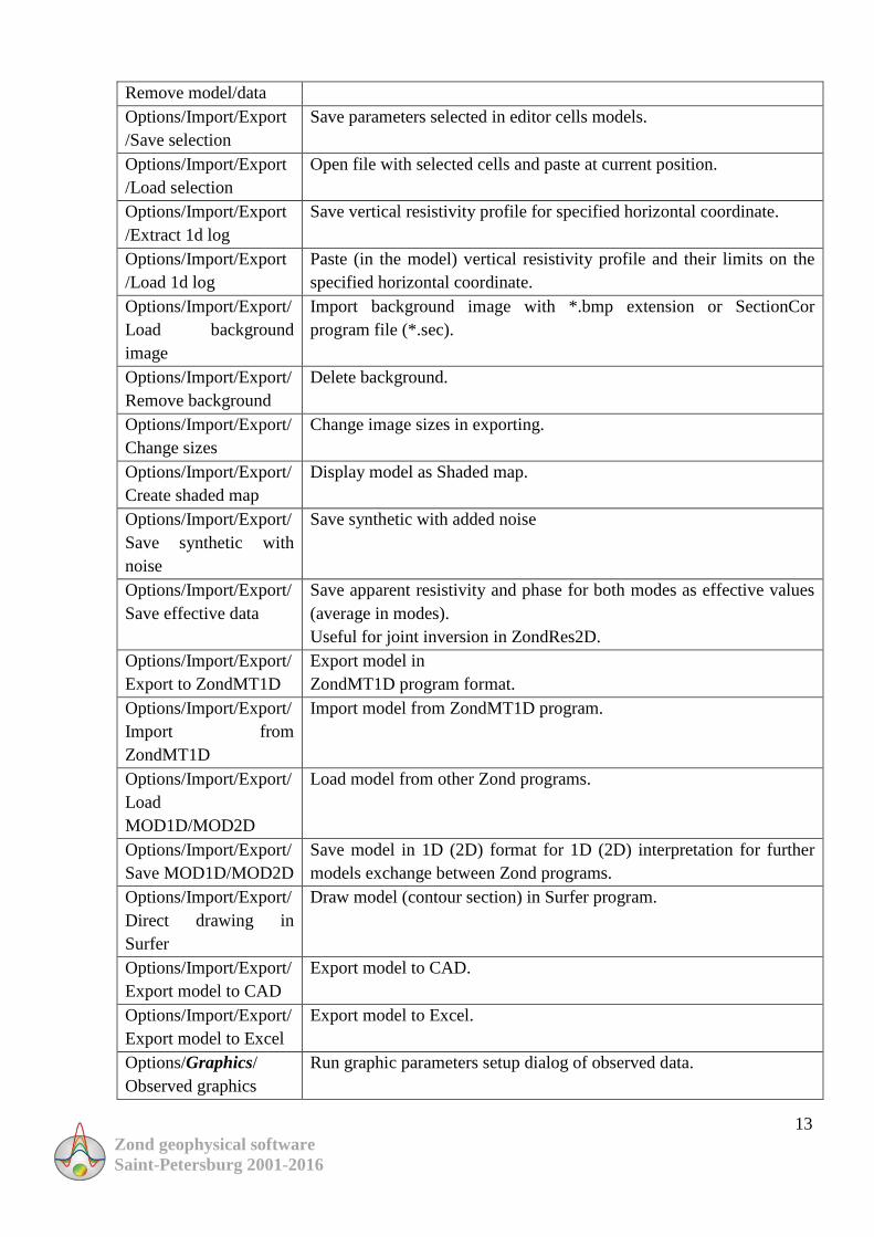
13



Remove model/data


/Save selection

Save parameters selected in editor cells models.


/Load selection

Open file with selected cells and paste at current position.


/Extract 1d log

Save vertical resistivity profile for specified horizontal coordinate.


/Load 1d log

Paste (in the model) vertical resistivity profile and their limits on the

specified horizontal coordinate.

Options/Import/Export/

Load background

image

Import background image with *.bmp extension or SectionCor

program file (*.sec).


Remove background

Delete background.


Change sizes

Change image sizes in exporting.


Create shaded map

Display model as Shaded map.


Save synthetic with

noise

Save synthetic with added noise


Save effective data

Save apparent resistivity and phase for both modes as effective values

(average in modes).

Useful for joint inversion in ZondRes2D.


Export to ZondMT1D

Export model in

ZondMT1D program format.


Import from

ZondMT1D

Import model from ZondMT1D program.


Load

MOD1D/MOD2D

Load model from other Zond programs.


Save MOD1D/MOD2D

Save model in 1D (2D) format for 1D (2D) interpretation for further

models exchange between Zond programs.


Direct drawing in

Surfer

Draw model (contour section) in Surfer program.


Export model to CAD

Export model to CAD.


Export model to Excel

Export model to Excel.

Options/Graphics/

Observed graphics

Run graphic parameters setup dialog of observed data.

14



Options/Graphics/

Calculated graphics

Run graphic parameters setup dialog of calculated data.

Options/Graphics/

Colorscale from PS

Copy pseudosection color scale.

Options/Graphics/

Smooth contours

Smooth model contours in the corresponding displaying mode

(Contour section).

Options/Graphics/

Smoothness

Set model smoothing degree in displaying (when working in Contour

section mode).

Options/Graphics/

Display every n point

The frequency of points displaying on apparent parameters sections.

Options/Graphics/

Bitmap output settings

Export image settings.

Options/Buffer/Model Save model in buffer or paste from it.

Options/Buffer/Open Display all buffer models.

When going into the polygonal modeling window (toolbar button of the main

window) the following options are available:

Modeling/Load background Import background image from *.bmp file or SectionCor program

document (*.sec).

Modeling/Show

background

Display background.

Modeling/Remove

background

Hide background.

Modeling/Get values from

background

Set polygon parameters (resistivity, polarisability) values of

corresponding block model cells (from results of preliminary

inversion or modeling).

Modeling/Set values to

background

Set polygon parameters (resistivity, polarisability) to

corresponding block model cells.

Modeling/Remove all

polygons

Delete all polygons.

Modeling/Save polygons Save polygonal model as *.poly file.

Modeling/Load polygons Load polygon model (*.poly file).

Modeling/Export to CAD Export polygonal model as DXF (AutoCAD) file.

Modeling/GraviMagnetic/

Load new data

Load measurements of magnetic and (or) gravity field.


Add new data

Add new data of magnetic and (or) gravity field measurements.


Field settings

Set parameters of normal magnetic (gravity) field, survey

parameters.


Substract median grav

Substract median from the set values of the gravity field, it means

to lead to the anomalous field values.

Modeling/GraviMagnetic/ Substract median from the set values of the magnetic field, it

15



Substract median mag means to lead to the anomalous field values.


Inversion

Start polygonal inversion of gravity\magnetic data (parameters

inversion for specified parameters).


Display GM window

Open window of displaying gravity\magnetic field measurements.

Modeling/Display color

scale

Display color scale of resistivity\polarisability.

Modeling/Colors from color

scale

Assign colors to polygons corresponding to a color scale

(alternative to set colors manually).

Modeling/Exit from

modeling mode

Exit from polygonal modeling mode.

“Hot” keys

Cursor pad /cursor in model editor Change active cell of the model.

Delete / cursor in model editor Clear active cell.

Insert / cursor in model editor Insert current value to active cell.

F / cursor in model editor Fix active cell value.

X / cursor in model editor Use “magic wand” tool to select domain (domain with

specified parameter value will be highlighted)

V / cursor in model editor Delete selected.

Up/down / cursor in model editor Change current value.

Space Calculate forward problem.

Status bar

Status bar is divided into a few sections which contain different information:

Cursor and active cell coordinates.

Active cell parameters.

Model editor mode.

Process indicator.

Relative misfit.

Additional information.

Misfit is the most important parameter from the list. Averaged relative misfit (in

percents) is calculated taking into account all measurements of current model. Other misfit type

is used for inversion; it includes data of model smoothness. It can be seen during inversion.

Adjusting starting model mesh settings

16



When file is successfully loaded, starting model setting dialog appears (Fig. 2), in which

it is possible to choose the mesh parameters and the resistivity of the starting model.

Vertical nodes field contains options which set vertical grid parameters of the model.

Program automatically selects these parameters using the following rules:

• Depth of bottom layer is equal to half of maximal pseudo-depth for used measurement

system.

• Number of layers is equal to double quantity of unique measurement periods but does

not exceed 40.

• Thickness of the next layer is 1.2 times more than the previous one.

Interpreter can change these parameters due to his concept of depth and details of

investigation.

Start height – sets thickness of first layer. This value must be approximately equal to the

width of the cell and necessary model resolution.

Maximal depth – sets depth of bottom layer. It should be remembered that the maximal

depth value must not be too large because influence of geoelectrical section parameters decreases

with depth. Maximum depth should specified proceeding from effective field penetration depth.

Layers number – sets number of model’s layers. Usually 12-14 layers are enough for

model description. It is not advisable to specify large values for this parameter because

computation speed will decrease.

Incremental number – sets ratio between thicknesses of adjacent layers. This parameter value

usually ranges from 1 to 2.

Horizontal nodes field contains options which set horizontal grid parameters

Fig. 2 Starting model setup dialog

17



Minimum – sets minimal coordinate of the profile.

Maximum - sets maximum coordinate of the profile.

Intermediate nodes – sets number of complementary nodes between two adjacent sounding

points on profile (0 – 4). It is recommended to specify 1 or 2 complementary nodes between

adjacent stations.

Half-space resistivity – sets resistivity of starting model.

Regular mesh – starts horizontal mesh construction algorithm, and complementary nodes are

selected from condition of split uniformity. This option should be used if distance between

adjacent stations is very different (It is advantageous for the accuracy of forward and inverse

problem solutions).

Press Apply button when mesh setup is finished, and the program starts work mode.

Model editor functions can also be used to correct mesh: add or delete intermediate

nodes, level cell height and width (more details in «Model editor»).

18



Main data file format

Program presents universal data format which contains information about coordinates and

relative elevations (in kilometers) of sounding sites.

Data format of the program.

First line contains sequence of periods (in seconds) during which measurements where

conducted (in increasing order).

It is followed by information about every sounding site on profile, divided in blocks

described below.

Block of sounding location description

First line indicates start of sounding site description (must contain «{» symbol).

Second line contains complementary sounding parameters.

First record is sounding site coordinate on profile, second is relief excess.

Third to sixth lines contain field measurements.

Each line must start with code-key which shows to the program what type of data follows

this key. Code-keys which control type of data have the following values:

First option of setting keys:

«Ro_a» – apparent resistivity.

«Phi» – impedance phase (in degrees, positive value).

In this case polarization type is unknown. Such data can be used to work in magnetic

and/or electric polarizability modes. Example-file sample_with_unidata.

«_w» – measurement weight.

Second option of setting keys:

«Ro_a_tm» – apparent resistivity for magnetic polarizability.

«Phi_tm» – impedance phase for magnetic polarizability (in degrees, positive value).

«Tm_w» – measurement weight for magnetic polarizability. If measurement errors are

not known, program automatically sets weight “1” for every measurement. Example-file

sample_with_tmdata.

Third option of setting keys:

«Ro_a_te» – apparent resistivity for electric polarizability.

«Phi_te» – impedance phase for electric polarizability (in degrees, positive value).

«Te_w» – measurement weight for electric polarizability. If measurement errors are not

known, program automatically sets weight “1” for every measurement. Example-file

sample_with_tedata.

Number and order of records in lines must strictly correspond to acquisition geometry

described in the first line of the file. If measurements at some periods are missing, their values

are replaced by «*» symbol. If there are no data about impedance phase, the whole line is

excluded.

Last line indicates end of sounding site description (must contain «}» symbol)

Column of complementary horizontal grid nodes can be added after description block if

necessary. Coordinate of every new node is entered after *** symbol. Complementary nodes are

usually added for model extension over last stations or if there is sharp relief beyond profile.

Example-file sample_with_ext_nodes.

19



It is preferable to record stations in the same order as on profile (in increasing order of

coordinate).

For correct work of the program data file must not contain:

incorrect symbols of records separator (TAB and SPACE use only);

absurd data values (for example, negative values of apparent resistivity).

It is recommended total record number should be no more than 5000 in one file.

Data file can be created using Zdconvert program supplied with inversion program.

Procedures of work with this program are described in Appendix 8.

Preparing data for inversion

Processing magnetotelluric data is divided into three phases: viewing and editing of

recorded electromagnetic field time series, obtaining transfer functions, post-processing. The

first two stages are generally done in software supplied with the MT equipment. ZondMT2D

allows performing the post-processing.

Post-processing (the final stage of data preparation for inversion) includes the following

set of procedures (where appropriate): viewing, estimation of quality, editing, transfer functions

smoothing, impedance polar diagrams building, the rotation of the impedance tensor,

suppression of static shift effect.

These procedures are implemented in the program in the form of individual functions,

which can be used in the process, and as a part of module of quality control and data editing MT

Editor, which is a collected in single window complete tools set for post-processing of the MT

data.

Options for data measurements editing

Measurements editor

To view and edit of individual measurement values of apparent resistivity, phase and

weight in a table use measurements editor. Measurements editor run by tab Options/Data

Editor, or by pressing the button on the toolbar. The tab includes a table that allows setting

each measurement (Fig. 3).

20



The table contains 9 columns:

ID Measurement index

X,km Location of sounding sense.

T,s Measurement period.

ρα Calculated value of apparent resistivity for magnetic polarizability.

φ Calculated value of impedance phase for magnetic polarizability.

Weight Measurement weight for magnetic polarizability.

ρα Calculated value of apparent resistivity for electric polarizability.

φ Calculated value of impedance phase for electric polarizability.

Weight Measurement weight for electric polarizability.

The last six columns, if it is necessary, can be edited using the keyboard. Absurd values

for the apparent resistivity or phase should not be entered. Measurements weights are specified

in the range from 0 to 1.

When moving the cursor in the table, the position of the active measurement is displayed

on pseudosections or graphics plane.

Sounding curves view and edit dialog (Sounding curves)

Press button in the toolbar of the main program window to run sounding curves view

dialog (fig. 4). This dialog allows browsing measured (continuous line) and calculated (dashed

line) sounding curves for TM and TE modes for each sounding site. The dialog also allows

browsing calculation results of 1D forward problem for local model of active station.

Fig. 3 Table of measurements editor

21



Toolbar of Sounding curves dialog contains the following buttons:

Start browsing sounding curves of previous point.

Start browsing sounding curves of next point.

Calculate 1D forward problem for current point of local model (1D layered model directly

under sounding site). Modeling can be useful if it is necessary to estimate degree of

medium “two-dimensionality”. Sometimes it helps to find out if phase is correctly

specified (in necessary quadrant).

Fix minimum and maximum values on axes. After fixing axes limits do not vary when

changing points. Axes limits can be also specified in axis parameters setup dialog.

Open list of advanced options

Advanced options are:

Invert this station Sets use or not current point in inversion. If data at the point has intense

noise, it can be ignored in inversion.

With static shift Draw theoretical Rho apparent curve taking into account fitted p-effect

value. This option is necessary for displaying curves after inversion, if

static effect was to be found for each curve.

BI-logarithmic Set bi-logarithmic scale.

Phase axis [0-90] Set phase range from 0 to 90.

Error gates Display weights.

Fig. 4 Sounding curves view and edit dialog Sounding curves

22



Remove mode Turn on the option of removing points.

Select mode Turn on the option of selecting points.

Process together Take action for resistivity and phase simultaneously (when selecting or

deleting point on a curve, the corresponding point is selected or deleted on

another curve).

Calculated-

Observed

Replace measured values to calculated values.

1D local field Calculate 1D forward problem at the current point for the local model (one-

dimensional layered model directly under the sounding point). Modeling

can be useful when it is necessary to estimate the degree to which curves

are "two-dimensionality" rather than 1D. Sometimes it helps to determine

whether the phase is correctly set (in the required quadrant).

Original data Return to raw data.

As can be seen from the additional options, window allows also data editing. To do it, use

the “circle” tool. To run it, turn on Select mode option (to select) or Remove mode (to remove).

Circle radius can be changed by the mouse wheel. Using the circle, it is possible to remove a

point (the center button), to increase (right button) and decrease (left button) point weight in

inversion. Point weight – is the reciprocal of the measurement dispersion and it is indicated in

the program in the statistical goal form. The larger the bandwidth, the less influence this point

has for the resulting model.

It is possible to edit the vertical and horizontal axes. To run parameters axes settings

dialog right-click the mouse while holding the SHIFT button on the selected axis (see the part

Axes editor).

Editing data dialog Data distribution

Data distribution dialog allows rejecting frequencies with low number of measurements

and thus quickening interpretation process. Dialog is accessible in the main program menu

Options/Advanced/Data distribution.

Using this option allows estimating number of sounding points on the profile, on which

data of specified period exist.

Figure 5 shows an example of using Data distribution function for rejection of

frequencies with small amount of data. There is a table in the left part of function dialog window

(fig. 5 B) which contains the following columns: N – order number of period, T – period, nTM –

number of points on current period for TM mode, nTE - number of points on current period for

TE mode, X – select/deselect period. Data distribution for each period is displayed as bar charts

in the right part of the window.

In this example several points have data on low frequencies (fig. 5 A). These data lead to

calculation time increase. In order to delete periods and decrease calculation time select them in

the table and press button in the left upper corner of the bar chart. The example (fig. 5 B)

shows that low-frequency measurements observed only in several profile points were rejected.

23



This dialog is an analog of Distribution mode tab MT Editor.

Fig. 5 Example of Data distribution function usage for rejecting unreliable data. A-B –

pseudosections of apparent resistivity before and after usage of Data distribution function

respectively, B – Data distribution dialog window

Б

24



Module of quality control and data editing

For quality control and data editing a special module is available in the ZondMT2D

program. To run it, select in the menu Options/MT Editor. The module allows performing all

basic post-processing operations of MT data.

Tab Data of MT Editor module consists of two parts (Fig. 6): the top and the bottom. The left

side of them contains graphs of the selected parameter distribution along profile, the right side

displays the curve for the selected parameter at the point indicated on graphs by red dotted

vertical line. Parameters displayed on the top and the bottom of the window are selected,

respectively, by buttons and .

In the example shown in fig. 6 in the upper window part graphs of apparent resistivity for

TM mode on the profile are displayed. Each graph corresponds to an individual frequency. List

of graphs is located in the right part of the window and allows disabling or adding various

frequencies curves. The red vertical line defines the current point for which on the right side of

the window (in the example - Station 14, 28_130) apparent resistivity curve is displayed. The

points list in the right window part allows attaching graphs to other selected points. To move

between the profile points, use the buttons and or just click on the graph point. When the

option Settings/Plots/P1 (P2) Multigraphics is turned on, curves for all points selected with the

Fig. 6 Data main window of MT Editor module

25



mouse on the graph, are displayed in the corresponding curves window (alternative way of

selecting curves in the list).

To display "gates" weights on the graphs, use option Settings/Display gates (Fig. 6).

Use the menu options Settings/Background data to display initial data graphs (before

editing) - Original data, calculated data - Calculated data or synthetic data for the model of

one-dimensional inversion - 1D inversion.

Parameters of lines and points are configured using the menu options Settings/Graphics.

To select points for editing on the curves and graphs, use tools or . Afterwards,

selected points can be further edited using the menu option Settings/Mode or :

Select/deselect Turn on/off mode of points editing

Edit points Allow editing points (moving)

Shift curve Turn on the mode of moving the whole curve (graph). Turn on the tool

when selecting the curve.

Shift selected Move all selected points

Edit gates Edit weights of measurements (gates)

Remove points Delete points

Smooth points Smooth

Interpolate Replace selected points by interpolation

Denoise Suppress noise

The other editing operations are made using menu items Operations:

Return to start data Return to the data before editing.

Return to original

data

Return to raw data

Remove selection Deselect

TM 1D smoothing Run 1D smoothing for TM mode data

TE 1D smoothing Run 1D smoothing for TE mode data

Fig. 7 Dialog of displayed parameters selection

26



TM smoothing

strong

Run strong smoothing for TM mode

TE smoothing

strong

Run strong smoothing for TE mode

P1 remove invisible Don’t display curve points, for which corresponding graphs are turned off

(in P1 window)

P2 remove invisible Don’t display curve points, for which corresponding graphs are turned off

(in P2 window)

TM correct phases

(0..90)

Reduce TM phase to 0-90 range

TE correct phases

(0..90)

Reduce TE phase to range 0-90

TM suppress shifts Suppress static shift of TM mode

TE suppress shifts Suppress static shift of TE mode

Apply inverted

shifts

Apply correction of static shift obtained by inversion results (after

performing inversion)

Exchange TM-TE Replace TM mode data to TE mode data (and vice versa)

Rotate dataset Rotate the coordinate system

Convert2impedance

s

Convert to impedance

Apply and close Apply changes and exit from editor

When not working with MT-field invariants, two-dimensional model coordinate system

should be oriented according to the longitudinal and transverse directions relative to the

structures strike. If the profile orientation does not satisfy this condition, during data file

opening, the program will report that it is necessary to rotate the coordinate system. This rotation

may also be needed when selecting areal data points for interpreted profile, or if significant

three-dimensional distortions exist. Appropriate assessments are based on the polar diagrams

analysis (tab Polar is described below), and the coordinate system rotation is carried out with the

option Operations/Rotate dataset. The rotation parameters are set in the appeared dialog (Fig.

8). It is possible determine rotation type, using Rotation tab (in a user-defined angle, according

to tensor main axes directions, maximum Zxy or phase tensor), on the Options tab - select a

frequencies range for which the turn with the specified parameters is made.

27



Tab Distribution allows estimating the distribution of data on the frequency in a

convenient way (Fig. 9). If there are too few data at any frequency, the data of the frequency can

be removed. It will accelerate the inversion process and help avoid additional errors. Each group

of columns of different colors corresponds to the period number (frequency). Each color

corresponds to the parameter specified in the legend on the right part of window. To delete data

for selected frequency, run menu by right-clicking on the appropriate column.

Tab Polar (Fig. 10) is performed to create impedance tensor and tensor phase polar

diagrams, needed to determine the dimensions of the studying medium and the needed to rotate

the coordinate system, the separation of regional and local effects etc. Polar diagrams are

constructed for each point and for each frequency. Different frequencies are displayed on the

Fig. 9 Tab Distribution of MT Editor module

Fig. 8 Dialog of selection of coordinate system rotation parameters

28



polar diagrams in different colors, as shown in the list on the left window part (if it is necessary

frequencies can be turned on and off).

To run menu of parameter selection, displaying in tab Polar, right-click in the upper

window part (in the header Impedance diagrams in Fig. 10):

Impedance

diagrams

Display impedance tensor polar diagrams

Phase tensor

diagrams

Display phasing tensor polar diagrams

Strike Display effective strike

Ind arrow Display induction arrows (tippers)

No norming Do not normalize values (diagrams radius)

Norming for frq Normalize by frequency

Norming for

frq/st

Normalize by frequency and reduce to unit (for all frequencies radius

values are equal)

Stations marks Display points locations

Frequency range Set frequencies range, for which diagrams will be created

Fig. 10 Tab Polar of MT Editor window

29



Determination of the selected processing parameters effectiveness often can be assessed

only by comparing them with each other. It is possible to store in a single project several data

processing variants in the ZondMT2D. This allows carrying out the data inversion using

different processing parameters, as well as returning to the saved variant or continue processing

from the saved phase in a single project. Saving of the data processing results is carried out using

the option Buffer of MT Editor window.

One can save the current processing results in four possible buffers in the pulldown list. If the

selected buffer already contains data (in this case, its name will be displayed with tick), the

program will ask about loading data from the buffer or rewrite the content of the current data.

It is possible to return to the raw data in the editing process (Operations/Return to start

data) or to the data taken from the buffer before they were changed (Options/Return to

original data).

Using the option Buffer of MT Editor window is similar to the procedure of working

with models based on the inversion results (Working with several models in a single project).

Static shift correction

Static shift caused by near-surface inhomogeneities, considerably complicate the

interpretation of the apparent resistivity curves, creating false geoelectric structures. The

reliability of data interpretation depends significantly on the quality of the static shift removal.

There are several features (instruments) for the detection and correction of static shift in

ZondMT2D program. In practice, the most efficient is to use all of these instruments, or at least

to compare their efficiency on real data.

Identification and manual correction of the static shift is carried out in the MT Editor.

Displaying a single window with several neighboring resistivity and phase curves allows visual

inspection of data for static shift effects. Using MT Editor tools, one can change the curve level

or its segments, with reference to the adjacent curves, calculated curves obtained by one-

dimensional inversion results or the calculated curves of the model obtained by the two-

dimensional inversion.

An alternative to manual correction in MT Editor module is a static shift correction by

averaging the apparent resistivity, with following filtration (module MT Editor, options TM

suppress shifts and TE suppress shifts). This method is effective in a dense observation grid.

The most reliable way to correct static shift is to use TDEM sounding data. TDEM data is

imported with the option Options/TDEM data/Load TDEM data (supporting formats are

ZondTDEM1D and UFS) in the ZondMT2D program. Also, it is possible to use for correction

VES data (imported into the project with the option Options/VES data/Load VES data. After

data importing, it is necessary to press the main menu button and go to the window of

determining the corrections for each point (Fig. 11). In the upper left window part displays

graphs of apparent resistivity on MT and TDEM, in the lower left - phase (observed and

calculated), in the upper right - depth curve (observed and calculated), in the bottom right -

geoelectric model of one-dimensional joint inversion.

30



The buttons and allow proceeding to the next or previous point. The button

runs the joint inversion process of MT and TDEM (MT and VES or MT, TDEM and VES). The

button determines the selection of TDEM points for the considered MT point and produced

action:

Rebuild Model Reset model

Any near

TDEM/VES point

Select any near TDEM point (for example, if there is only one or two

points on the profile)

Nearest TDEM/VES

point

Select nearest TDEM point

Invert only visible Include to inversion only visible parameters (selected by “tick” under

each graph)

Invert thicknesses Run thickness inversion

Apply static shift

TM

Apply static shift correction for TM mode

Apply static shift TE Apply static shift correction for TE mode

Phase correction TM TM phase correction

Phase correction TE TE phase correction

Auto correction When option is turned off, program ask user confirmation

After clicking the option Apply static shift TM and Apply static shift TE the

corresponding corrections will be entered in the data.

Fig. 11 Window of static shift correction based on of the TDEM and VES data

31



The button allows copying the model to the resistivity section. This allows setting the

model obtained by one-dimensional joint inversion of MT, TEM and VES results as a starting

model.

Apparent parameters visualization

In the main window the observed and calculated parameters can be displayed as

pseudosection Options/Data/Pseudo-section, and as graphics plot Options/Data/Graphics-plot.

Graphics plot

The graphics plot displays parameter values along the profile, in the graphs form (Fig.

12). Use mouse to work with graphics plot: Zooming in or moving part is performed with button

pressed (the tool - "rubber rectangle"). To select an area, which you want to zoom in, move the

cursor down and to the right, with the left button pressed (Fig. 13A). To return to the original

scale, do the same actions, but the mouse is moving up and to the left (Fig. 13B). To move

(scroll) graphic, move the mouse with the pressed right mouse button.

By pressing the left mouse button on the graph point makes the following actions: hiding

the rest graphics and displaying the electrodes position for the active point (until releasing the

mouse button). Editing the measured values is done by moving the graph point with the right

mouse button pressed.

Dialog of graphs plot settings is called from the Main Menu Options/

Graphics/Observed graphics Calculated graphics (described in Appendix 1). To run Graphics

editor click the right mouse button with pressed SHIFT key on the graph (described in Appendix

2). To run the axes editor right-click while holding down the SHIFT key on the axis (described

in Appendix 5). To run legend editor click the right mouse button while holding down the SHIFT

key on the legend to the right of the graph (described in Appendix 3).

32



To select one and, accordingly, the removal the other graphics click on the legend while

pressing SHIFT. Two click for inverse action.

To scroll through the graphs use the mouse wheel. Select several adjacent plots (in the

legend) and scroll the mouse wheel, moving the cursor to the legend. Activity graphs indexes

will vary. When right-clicking on the graph point measurement will be highlighted in the table.

It is possible to exclude some measurements from processing specifying 0 as the weight

in the mode of graphs data displaying. A separate measurement can be deleted by pressing the

ALT key and the left mouse button on the graph point. Click the right mouse button and ALT in

the graph to specify weight 0 for all graph measurements.

If the measurement weight values are specified in the input data file, it is possible to

display an appropriate range of the resistivity values in the graphs (confidence interval) using the

Fig. 13 The direction of mouse movement when zooming

Fig. 12 The main program window. Displaying data as graphics plot

Б

33



option Options/Data/Display/Error gates. Confidence intervals (weights) can be adjusted in the

graphics mode by pressing the left or right mouse button while holding down ALT.

Pseudosection

Pseudosection visualizes parameter distribution along profile with depth (fig. 14).

Plotting in form of contour lines has axes: measurement coordinate along profile,

pseudodepth. The color scale sets ratio between the displaying value and color.

Double click next to object axes runs context menu which contains the following options:

Log data scale Use logarithmic scale on colour bar.

Smooth mode Use smoothing interpolating palette/contour section.

Display grid point Display measurement point ticks.

Display ColorBar Display colour scale.

Setup Run pseudosection parameters setup dialog.

Print preview Print pseudosection.

Save picture Save pseudosection as *.emf graphic file.

Save XYZ file Save pseudosection as *.dat text file.

Default Set pseudosection parameters on default.

Pseudosection parameters setup dialog is described in Appendix 4 Appendix 1: Graphics

editor. Axes editor is called by right-clicking while holding down the SHIFT key on the axis

Fig. 14 The main program window. Displaying data as pseudosection

34



described in Appendix 5. Editor pseudosection points can be called by clicking the right mouse

button while holding down the SHIFT key at the point (described in Appendix 7).

When displaying data as pseudosection it is possible to view the data of the individual

settings using the menu Options/Data/Display/. When there are large measurement volumes it is

possible to thin pseudosection points using the option Display every N point. By default, this

option is turned on when loading a data file that contains more than 3000 measurements.

To display measurement weights as pseudosection in the middle program graphic section

use the option Options/Data/Data Weights and after the inversion process relative error for

each measurement by Options/Data/Data Misfit.

Input and editing topographic information

There are two ways to input relief - through the information in the input data file or by

using the option of topographic information import of the main menu

Options/Topography/Import topography. Importing topographical information is done from a

text file that contains two columns: the distance on the profile and elevation. Option

Options/Topography/Import topography creates a table with information from the selected

text file is loaded (Fig. 15). X and Alt must be selected in names of the corresponding columns

(to do it make active the cell with column name, press the left button to appear a list of columns

names). To end the topographic information input press the button .

Menu item Options/Topography/Edit topography calls a dialog that allows editing

topographic information (contained in the source data file or importing to the project) using the

table.

Use the menu items Options/Topography/Restore topography and

Options/Topography/Remove topography to recover and remove, respectively, topography

data.

When working with data obtained in the rugged area, it is recommended to use the option

of topography smoothing (Options/Topography/Smooth topography). Turn the option on

before opening a data file.

Fig. 15 Table of topographic information import

35



If it is necessary to take into account the relief forms outside the area, it is possible to add

additional nodes to the model edges using the option Options/Extra/Extended nodes. Turn the

option on before opening a data file.

When working with data it is sometimes convenient to disable the relief – by using the

option Options/Topography/Remove topography. To restore the relief use the option

Options/Topography/Restore topography.

To edit topography data use option Options/Topography/Edit topography.

By default, relief heights are displayed relative to zero in the model window, when the

option Options/Topography/Absolute coordinates is turned on. Specified in the file relief

heighs are displayed.

When saving Grid file with real heighs in the exported file option Absolute coordinates

must be turned off.

Relief distortion factor with the depth (0-5) can be set in menu

Option/Topography/Topo coefficient. 0 - the relief of each next layer repeats the previous one.

1 - relief flattens with depth, the last layer - flat (Fig. 16). Distorted depth is calculated as

follows:

Tcoeff

z

xTopoTopozxTopozxz

)max(

)max(1,* ,

where Topo - relief excess, z - depth from the surface.

Fig. 16 Model layers distortion with Topo coefficient parameter values of 1 to 5

36



Data inversion

After loading the data file, setting the starting model, data editing and input topographical

information it is necessary to select the inversion type and set inversion parameters. Also, if it is

necessary, it is possible to calibrate the model grid, its editing and changing of the starting model

resistivity values (described in the model creation). The program supports two basic modes of

inversion: in the block model (if this option is turned on), and in layered medium model (if

this option is turned on). To run inversion parameters setup dialog click the button or use

menu item Option/Program setup.

Rapid assessment of the inversion results can be given by the value of the relative

discrepancy in the program status bar. As a rule, the "average" as the data value must not exceed

5%.

Convergence of each measurement between the observed and calculated values can be

evaluated by displaying pseudosection of relative discrepancy with the option Options/Data /

Data Misfit.

Calibration of model mesh and operations with relief

One of the most important aspects of successful forward and inverse modeling is correct

selection of model mesh. Mesh must ensure exact solution for each frequency. Forward

modeling is calculated on conditions that electromagnetic field in every cell of the section

changes linearly. It is known that field nonlinearity degree decreases with depth but in different

ways for each frequency. Geoelectric contrast of objects is an important factor that influences

field behavior. That is the reason why mesh needs to be more concentrated within the bounds of

these objects to receive more precise modeling results. But for discretization parameters model

quality also depends on how far “infinite” boundaries that ensure fulfillment of conditions at

infinite are moved away. And in its turn this depends on size of visible region of the model. In

other words external mesh is set on the basis of parameters of inner, specified by user mesh.

In order to raise reliability of received data model mesh calibration should be performed.

Calibration is carried out for half-space model without relief. When starting model is created,

press button of forward modeling in the toolbar. A criterion of proper mesh selection is

closeness of all calculated apparent resistivity values (for both modes on each frequency) to

resistivity of half-space and closeness of phases to 45 degrees.

If strongly variable topography is present, it is helpful to add 1-2 complementary nodes in

the upper part of vertical grid (more details in Model editor). If forward solution does not change

much because of this, it means that mesh is created properly.

Program parameters setup dialog

This dialog serves to specify parameters of inverse modeling. Use Options/Program

setup option in the main menu or button in the toolbar to run it (fig. 17).

First tab Inversion serves for inversion parameters adjustment.

37



Inversion option selects algorithm of inverse modeling. Let us consider inversion

algorithms by example of subsurface model that consists of several blocks (fig. 18). For

algorithm testing theoretical response should be calculated and 5 percent Gaussian noise

superimposed.

Smoothness constrained is inversion by least-square method with use of smoothing

operator. As a result of this algorithm smooth (without sharp boundaries) and stable parameter

distribution is received (fig. 19). This type of inversion is recommended in the majority of cases.

Matrix equation for this kind of inversion is the following:

fWAmCCWAWA TTTTT (9)

Fig. 18 Test subsurface model

Fig. 17 Inversion parameters setup dialog, Inversion tab

38



Occam is inversion by least-square method with use of smoothing operator and

additional contrast minimization. As a result of this algorithm the smoothest parameter

distribution is received (fig. 20). Matrix equation for this kind of inversion is the following:

CmCfWAmCCWAWA TTTTTT (10)

Marquardt – classic inversion algorithm by least-square method with regularization by

damping parameter. This algorithm allows receiving model with sharp boundaries (fig. 21).

Unwise usage of this inversion method modification can lead to receiving unstable results and

increasing of RMS deviation that is algorithm discrepancy. The best option is to use Marquardt

method as specializing after Smoothness constrained or Occam inversion is performed. Matrix

equation for this kind of inversion is the following:

fWAmIWAWA TTTT (11)

Fig. 20 Regenerated model as a result of Occam inversion

Fig. 19 Regenerated model as a result of Smoothness constrained inversion

39



Blocks – fits parameters for certain domains which differ in resistivity. Domains with

equal resistivity consider as single blocks (fig. 22). It is preferable to use this algorithm for

specifying results of previous methods when necessary blocks are have already been selected.

Focused is inversion by least-square method with use of smoothing operator and

additional contrast focusing. As a result of this algorithm piecewise smooth parameters

distribution (that is model which consists of blocks with constant resistivity) can be received (fig.

23). This algorithm is sensitive to threshold parameter. In other words this parameter defines if

adjacent cells are unified or not. If contrast of adjacent cells is higher than specified value then

cells parameters are averaged weakly, if lower – strongly. Matrix equation for this kind of

inversion is the following:

RCmCfWAmRCCWAWA TTTTTT (12)

Stop criteria field contains inversion stopping criterion.

Fig. 23 Regenerated model as a result of Focused inversion

Fig. 22 Regenerated model as a result of Blocks inversion

Fig. 21 Regenerated model as a result of Marquardt inversion

40



Iterations – if this function is ON inversion process stops as soon as specified iteration

number is reached.

RMS error – if this function is ON inversion process stops as soon as specified RMS

level is reached.

Reduction – if this function is ON inversion process stops as soon as RMS error

increases repeatedly for two sequential iterations (on selected value, in percents).

Model field common limits (Min resistivity, Max resistivity) – set model parameters

limits of variation for inversion. It is very important to constrict parameters range of variation. It

makes resultant model more stable, on one hand, and allows receiving more adequate results

from geological point of view, on the other.

Tab Model (fig. 24) contains additional inversion settings

Option Smoothing factor – Smoothing factor sets dependence of measurement misfit

minimization on model misfit. In case of noisy environment or in order to receive smoother and

more stable parameters distribution quite high smoothing parameter value is chosen: 0.5 – 2.0;

0.005 – 0.1 values are used for high quality data. High smoothing parameter values mostly lead

to high data misfits (fig. 25). Smoothing factor is used in Occam and Focused inversion

algorithms. But for model smoothness this parameter also allows stabilizing inversion process

which is very important if data has considerable component of noise.

Depth smoothing - sets the attenuation factor (smoothing) with depth. The parameter

value also depends on the noise level - at a high level and the appearance of the inversion

Fig. 24 Inversion parameters setup dialog. Tab Model

41



"ungeological" objects this parameter should be increased in the lower part of this section. The

value is chosen empirically.

Smoothness ratio – specifies smoothness ratio in horizontal and vertical direction. Set

this parameter larger than 1 for vertically-layered subsurface and smaller than 1 for horizontally

stratified earth. Usually this parameter value ranges from 0.2 to 1 (fig. 25).

Option Focused Threshold – defines threshold contrast value for adjacent cells, and if it

is reached adjacent cells parameters are not averaged (it is considered that there is a boundary

between these cells). This parameter value is chosen empirically (0.001-1). Small parameter

value can cause algorithm discrepancy (in this case it needs increasing). Large value leads to

receiving smooth distribution (fig. 26).

Number of surface layers (0-2) – sets number of layers in which strong variation of

parameters is possible. Use 1 or 2 layers if near-surface section is very heterogeneous and it has

negative effect on the whole section. If this option is used the majority of heterogeneities are

concentrated in hear-surface layer and bottom part of the section is smooth after inversion.

Fig. 26 Geoelectric models as a result of Focused inversion with Threshold parameter: 0.01

(A) and 0.1 (B)

Fig. 25 Geoelectric models as a result of “smooth” inversion with Smoothness ratio parameter: 1

(A) and 0.3 (B)

B

42



Cell grouping – use this function for big models (when opening files with large number

of data values, program automatically offers to use this function). It activates table that allows

merging adjacent cells and receiving less number of determinate parameters for inversion. When

using this option, the cells number for the direct problem solution remains the same, while the

number of cells for the inversion is reduced. Ideally, the amount of adjustment parameters should

be close to the amount of data.

The table contains three columns. Number of initial model layer is specified in the first

column (Layer). Number of inversion mesh layer is contained in the third column (New layer).

Number of cells (in horizontal direction) that contain in every cell of inversion mesh for current

layer is set in the second column (Width). Inversion mesh is displayed in model editor during

setup. Double left click on cell in Width column to merge cells in horizontal direction for

current layer, right click – to run dialog to set layers number for merging. It is applied for current

and all lower layers. Merging cells in the vertical direction is carried out in a similar way when

working with the column New Layer.

There are three examples of inversion meshes below: in the first picture inversion mesh

corresponds to model one (fig. 27A); in fig. 27 B cells starting from the second layer merge by

two in horizontal direction; in the third picture cells starting from the sixth layer merge by two,

but from the twelfth by four in horizontal direction (fig. 27C).

The similar functions are run by the option Options/Cutting. If the Cell grouping is

created to merge cells in the "middle" profile part, then Options/Cutting angle allows doing this

for the edge section fields (Fig. 27 shows active cutting option for all models).

Options located in the tab Data (Fig. 28), allow choosing which data should be used in the

inversion, set the data types weight and type of data normalization.

Fig. 27 Examples of inversion meshes

B

C

43



The table on the tab Data contains the columns, corresponding to the data type name (#),

a field that indicates taken into account or not data in the inversion (Invert), the data weight

(Weight), minimum and maximum frequency (minfq and maxfq).

Option ABS allows using the parameter module in the inversion.

When the option Effective impedance (D) is activated, effective impedance inversion will be

made.

Robust weighting scheme – this option should be turned on if there are individual high

deviations caused by systematic measurement errors. It is important to note that this algorithm

should be used iа there is no more than 30 % of rejected data. If noise constitutes the most part of

data this algorithm is hardly helpful.

Data type – sets type of data normalization for inversion. Log(rho)&linlog(phase) is

recommended. It usually leads to the best inversion algorithm convergence.

The program supports two basic modes of inversion: in the block model (if the option

is turned on, the examples are shown above), and in random-layered medium (if the option is

turned on, described below). It is possible to do joint inversion of MT data and the data of

transient electromagnetics (Options/TDEM data/Invert TDEM data), as well as set results of

the joint one-dimensional inversion of MT, TEM and VES as a starting model for the inversion

(produced in the SSC). Option on the main program window toolbar allows making

conventional one-dimensional inversion.

Inversion in layered medium

Option of the main program window toolbar allows making inversion in arbitrarily-

layered medium model. In this mode, user determines layers number in the resulting model and

Fig. 28 Dialog of inversion settings. Tab Data

44



sets parameters that determine the rate of boundaries position changing and defined layers

properties.

To run starting model setup, use option Options/Mesh constructor, as in the grid mode

(Fig. 29).

Start thickness parameter determines the first layer thickness, Layers number - the

number of layers, Thickness factor - magnification factor of the underlying layer thickness.

Geometry nodes specifies the number of points, which are contained boundary. During the

inversion program will change the boundary form due to the vertical shift of these points.

Accordingly, the more points, the more "smooth" boundary will be available as a result of

inversion.

Par value defines the resistivity value of the first layer. Parameter Par nodes 1 layer defines the

boundary nodes (points) number, in which selecting parameter (resistivity) can be changed. If set

to one, the resistivity will be the same for all layers. If the value is two, the resistivity will vary

linearly from the left layer boundary to the right. The same parameter for other layers is set in the

field Par nodes 2-n layers. To apply described above parameters changes to the model, press the

button .

Table of starting model setup window is used to display and modify parameters for each

layer separately. Activate option for Z to jump thickness values to the depth values.

Example of inversion results in the layered model is shown in Fig. 30 and Fig. 14.

Fig. 29 Starting model setup dialog window in the mode of working in layered model

45



Incorporating a priori information in the inversion

Inversion can be carried out without a priori information (pure transformation) and taking

into account prior information (in this case interpretation element is added to the transformation).

The incorporation of a priori information in the inversion is most often performed in two ways:

by specifying the starting model (hypothetical choice of resistivity section) or by the tear

boundaries position.

By default, the starting model for the inversion is the current ZondMT2D model, which is

displayed in the model editor. It will be changed in the inversion. Model obtained in the

inversion depends from the model type of starting model. The similarity degree is determined by

the parameter Smoothing factor in the inversion settings window. The higher the Smoothing

factor value, the less the result will be different from the prior model.

Contrasting boundaries position, obtained by borehole and other geophysical methods is

set by using the toolbar, called by the menu item Options/Inversion/Set boundaries.

Boundaries editing and accounting in the inversion is made when the button is pressed. To

add the boundary points left-click mouse button while pressing the button . To end adding

boundary points right-click. Then it is possible to start adding the next boundary or starting

inversion. When defining boundaries it is recommended that they, whenever possible, do not

cross cell edges. To remove the boundary right-click with the button being pressed.

Boundaries can be saved and loaded.

Example of models obtained by inversion without and with taking into account

boundaries shown in Fig. 32.

Fig. 30 Inversion results in the layered model

46



Movies showing the process of taking a priori boundaries in inversion are available on

page http://zond-geo.ru/examples/video-lessons/ (http://zond-geo.ru/zmovies/Boundaries.exe

and http://zond-geo.ru/zmovies/BoundaryInversion.exe.

Program allows displaying a priori information on the section, which significantly

facilitates the creation of a resistivity reference model or boundaries setting. A priori information

displaying process is described in "Visualization of additional information"

Set boundaries dialog

Set boundaries dialog can be run using Options/Advanced function of the main menu.

It allows taking into account a priori geological information for inversion. When this tab is

selected, menu with the following buttons appears:

Enable/Disable editing boundaries mode Turn on/off editing boundaries mode

Add new boundary Add new boundary

Delete boundary Delete all boundaries

Save boundaries to file Save boundaries to file

Load boundaries from file Load boundaries from file

One of the most important ways to improve interpretation quality is implementation of a

priori geological boundaries to inverse problem. It increases problem stability, on one hand, and

decreases equivalence domain and allows receiving more consistent structure, on the other. In

these domains of the model where parameters are not sensitive this is almost the only way to

receive acceptable result.

It is preferable to use Occam algorithm if boundaries are implemented. Usually 1 or 2

boundaries are used, and it should be remembered that geological boundaries do not often

coincide with petrophysical ones.

It is recommended to perform inversion using Occam algorithm before setting

boundaries; then plot present borehole data on received geoelectric section. See details of

logging and lithology data file creation in «Borehole columns and logging data visualization».

Boundaries should be plotted on received geoelectric section with account of borehole

data and on the basis of a priori concepts of geological structure. Boundaries are set by left

mouse click with enabled editing boundaries mode. Right click to close the line. It is

recommended not to use many nodes when plotting the boundaries. It is advisable to plot the

smoothest boundaries close to inversion mesh modes.

Inversion should be run again when boundaries are plotted to take into account specified

boundaries (fig. 31).

http://zond-geo.ru/examples/video-lessons/

http://zond-geo.ru/zmovies/Boundaries.exe

http://zond-geo.ru/zmovies/BoundaryInversion.exe

47



Model visualization modes and parameters

The model can be displayed as cells Options/Model/Block-section (Fig. 32 A), in

a smooth interpolation palette Options/Model/Smooth-section (Fig. 32 B), and as a contour

section Options/Model/Contour-section (Fig. 32 C).

Fig. 32 Versions of displaying model: Block-section (A), Smooth-section (B), Contour-

section (C)

Fig. 31 Example of Set boundaries function usage. The middle section – geoelectric section

received using Occam algorithm without plotting boundaries, the button – geoelectric section

calculated after plotting boundaries

B

C

48



When you right-click in different areas of the model editor context menu appears with

the following options:

Top area near

«Resistivity block-

section»

Display model mesh Enable/disable model mesh display.

Display objects

border

Enable/disable objects border display.

Display color bar Enable/disable color bar display.

Setup Run model parameters setup dialog.

Zoom&Scroll Enable zoom and scroll mode.

Print preview Print model.

Color bar Set minimum Set minimum value of colour bar.

Set maximum Set maximum value of colour bar.

Set incremental factor Set minimum and maximum values of color bar

relative to host medium value.

Automatic Automatically set minimum and maximum value

of colour bar.

Log scale Set logarithmic scale for colour bar.

Set halfspace value Set host medium parameter value.

Set cursor value Set current parameter value.

Colors as histogram Set colors based on the distribution of the cell

model resistivity.

Section area Working with model

context menu

Described in «Working with block model»

Axes area Model editor Described in «Model editor»

When moving the mouse cursor within working windows, local window coordinates are

shown in the left section of the main window status bar.

Appendix 6: Dialog of model parameters displaying describes model parameters setup

dialog Setup (color scale, line thickness, etc.) when working in Block-section and the Smooth-

section modes. Work in the mode Contour-section is described in Appendix 4: Pseudosection

(contour section) parameters setup dialog (contour section).

Program additional features depend on the selected display mode of the model.

Mathematical modeling is more convenient to carry out in Block-section mode. Distribution of

integral sensitivity is displayed in the contour section (Contour-section) - option

Option/Model/Sensitivity. The potential distribution and the sensitivity function is displayed in

(Block-section) or in interpolation palette (Smooth-section).

The edges of the model have generally worse resolution. Very often the inversion results

in these areas contain many false anomalies. Option Options/Cutting allows hiding model edges

by setting the value (in degrees) of the trim angle (Cut by angle, Fig. 33) or sensitivity level

(Cut by sensitivity).

Option Options/Cutting/Extend bottom enables or disables the stretching of the lower

model cell.

49



Option Options/Import/Export/Create shaded map allows displaying model as a

shaded map (shaded map, Fig. 34).

Fig. 34 The main program window with the model image in shaded maps mode (shaded map)

Fig. 33 Models comparison with different cut angles (Options/Cutting/Cutting angle): A - no

trimming, B -angle of 30°, C - angle of 55°

50



Dialog Options/Extra/Model&Data histograms allows to display the plot of apparent

resistivity distribution in the data and distribution of the real resistivity in the model (Fig. 35).

Changing of the vertical line position allows specifying the minimum and maximum of

parameter color scale.

Interpretation results saving

Profile interpretation result is hold in « ZONDMT2D » file format (extension *. m2d).

Field data, relative measurement weights, and current subsurface model are saved in this file.

Data from the file are used for further load and subsurface model creation.

Use button in the toolbar or corresponding menu option File/Save file to save

interpretation result. This dialog also allows choosing file format to save observed (Observed)

and calculated for current model (Calculated) apparent resistivity values and images (Model,

WorkSheet) in *.BMP format (more details in «Exporting image setup dialog»). There a few

options to save data:

Zond MT project data Save observed data and current subsurface model.

Zond MT calculated data Save calculated data.

Zond MT observed data Save observed data.

Zond MT Model with

calculated

Save calculated data as observed data and current model.

Worksheet Save three graphic section of the window in BMP format.

Model Save bottom graphic section of the window in BMP format.

Program configuration Save program parameters.

Grid file Save current model as grid-file in DAT format. In addition for

further convenience bln file which contains characteristic relief

points is saved.

Section file Save current model in Section format.

Fig. 35 Window Histogram - the histogram of the data values and models

А

В

51



Modeling and working with model

Modeling is an important process that precedes the field work. It allows determining

feasibility to solve a geological problem with geophysical methods, as well as to select the

optimal survey layout parameters for it, to assess the signal level and the resolution of the

selected survey layout. Using a priori information the interpreter can model different geological

scenarios, planning geophysical work.

The program ZondMT2D allows modeling numerous practical applications of MT-

method in two dimensions, taking into account the profile relief (any applying practically

frequency ranges, an arbitrary profile step, block structure arbitrary model setting, polygonal

models creation).

Parameters of the survey layout and environment model are the necessary input data for

modeling. ZondMT2D allows creating observation systems and environment models in the

program as well as use the survey layout saved using other formats and create geoelectric models

based on other Zond programs and geological sections, defined as a background.

Survey layout definition

Observation (measurement) system or survey layout can be set in two ways: create it

directly in the program or load from the data (measurements) file.

Creating the survey layout in the program comes with the option File/Create synthetic

survey (Fig. 36).

Point number determines the number of observation points on the profile, Point

separation - the distance between the observation points in kilometers, Period number - the

number of frequencies (periods) of the sounding signal, Start period and End period -

respectively, the smallest and the largest period of the sounding signal.

After setting the parameters and clicking the button , dialog of grid settings Mesh

constructor appears (more details in «Starting model setup»).

Fig. 36 Dialog of synthetic survey layout creating

52



An alternative to creating measurement configuration directly in ZondMT2D is its

loading from a data file with various supporting formats. To do this, simply open the data file via

the main menu File/Open file. This option allows modeling for the measurement configuration,

which is used in field research, as well as set the survey layout with all sorts of settings.

For the further parameters changing of the observing system before opening the

measurements file it is necessary to go to the modeling mode: Options/Extra/Open in modeling

mode.

Model building in ZondMT2D

Geoelectric medium creation produced in the model editor - lower section of the

graphical window. The program ZondMT2D has two modes to create a model: block

(Options/Model/Block-section) and polygon (toolbar button ). The block mode is performed

for directly model cells editing (the width or thickness of the selected row of cells and cell

properties). Polygon mode is used to set the environment consisting of a set of related or

unrelated to each other bodies.

When working in block mode, it is also possible to edit some grid parameters created in

the dialog Options/Mesh constructor. They are described in the «Model editor».

It should be noted that any mode of creating models has developed work settings with a priori

information: loading of borehole and logging data, background as a raster file, models from other

ZondMT2D programs. These tools are described in the «Data import and export».

Model editor

Right-click on the vertical and horizontal axes in the model editor field options to edit the

grid created when working with dialog Mesh constructor appears.

Vertical axe

Log scale Set logarithmic scale to the vertical axe.

Set maximum Set bottom layer depth value.

Redivide Set equal thickness for all model layers (in current scale)

Thick mesh Delete every second node of vertical axe

Thin mesh Add intermediate nodes in vertical grid

Horizontal

axe

Redivide Set equal width of cells situated between unique positions of

sounding sites

Thick mesh Delete every second node of horizontal grid (if there is no

sounding site in this node)

Thin mesh Add intermediate nodes in horizontal grid

Working with block model

Block model editor is used to change the parameters of individual model cells using a

mouse. Working with model cells is like editing of raster image in graphics editors. When

moving the cursor in the model, the status bar at the bottom of the main window displays the

53



coordinates and parameters of the active cell in which the cursor is located. The currently active

cell is surrounded by a rectangle - the cursor. The selected or fixed cell is hatched with white or

black points.

To work with the block model, there are two tools sets in the program: the context menu

(right-click in the editing model), external toolbar (Options/Model/ModelEditor toolbar) and

color scale. The functions of context menu and external toolbar largely duplicate each other:

Context menu Model

tools Option

Zooming, scaling of a model

Display cell setup Run cell parameters setup dialog.

Cell to cursor

value

Use active cell parameter as current value

Edit mode

Run Edit mode

Selection\Free

form selection Highlight set of cells within edit region using mouse. Field is

limited by user.

Selection\Rectangu

lar selection Highlight set of cells within edit region using mouse. Field has

rectangular form.

Highlight set of cells within edit region using mouse. Field has

elliptic form.

Selection\Magic

wand

Highlight set of cells within edit region using mouse. Active cell

and adjacent cells whose parameters are close to its parameter are

highlighted. Proximity is specified in model parameters setup

dialog.

Selection\Remove

selection Delete selected

Mesh options\add

column /row Add new vertical or horizontal boundary. Click in necessary

point to creat new boundary there.

Mesh

options\remove

column /row

Delete selected vertical or horizantal axis

Mesh

options\resize

column /row

Change row or column thickness using mouse

Clear model Clear current model parameters

Clear parameters Clear resistivity values of the current model

The color scale, linking the color value with the value of the resistivity is on the right of

the model editing area. To select the current value left-click on the scale, and the value is

displayed below of the color scale. To change the cell parameter value left-click on the cell to

change its parameter to the current one.

The program has several modes of selecting cells to create a model quickly: by a

rectangle, by an ellipse, by free form and by for a specific parameter value. To the options use

54



the context menu by pressing the right mouse button in the editing model area, or as a separate

remote toolbar (Options/Model/ModelEditor toolbar). If a certain section area is highlighted,

then press the left mouse button anywhere in the selection area to set for all cells in the field the

current parameter value.

For example, to set certain resistivity value to rectangular area section, select this area

section using the tools described above, the left-click on the color bar (select the required

resistivity), and left-click in any point of the selection area, which then gets assigned the selected

resistivity value.

Zoom-in or moving of a section part is carried out in the mode Zoom&Scroll (is turned

on in the context menu of model parameters setup by right-clicking near the Resistivity block-

section in the model window) or after pressing the button on the panel Model tools. To

select the area to zoom in, the cursor moves down and to the right with the pressed left button.

To return to the original scale, the same actions, but the mouse is moving up and to the left.

To increase the cell parameter left-click the while holding SHIFT on the cell or cells

group. Right-click on the cell while holding SHIFT to decrease the cell or cells group parameter.

Percentage of parameter value changing sets in the dialog of model parameters setup. If the

active cell is selected, then all the above described operations are applied to the all selection.

Clicking the mouse while pressing CTRL allows moving selected cells set within the editing area

using the mouse. When moving the selection with pressing the left mouse button the contents of

the selected cells are copied to the new location. When moving the selection with pressing the

right mouse button the contents of the selected cells is cut and copied to the new location.

It is also possible to set the parameter value to the selected cells using the cell parameters setup

dialog Cell setup (Fig. 37).

Dialog is intended for selection or choosing the cell parameters.

Value - sets cell parameter value.

Fixed - fixes or frees cell parameter.

Min value, Max value – sets cell parameter size of changing.

The selected area is saved when going from the resistivity mode to the polarizability

mode.

55



To calculate the response of apparent parameters from a given geoelectric model (to solve

the forward problem), press the button on the toolbar.

To restore the original model, that is, to solve the inverse problem for the calculated from

the given model data, save the theoretical signals with filter Zond calculated data, and then

open as observed. To compare the restored and original models use the option

Options/Import/Export/Import model/data (Data import and export part), before it save the

original model by selecting the filter Zond model with calculated. A simpler way to compare

models is using the tool Bufer, it allows working with several models at the same time «Working

with several models in a single project» part).

Cell summarization dialog

Cell summarization (Options/Advanced) option serves to smooth (divide it into

blocks)or roughen current model. Block model can be used for inversion of Blocks type.

Selection of parameters for each block is performed then. Roughening process represents a

peculiar kind of rasterization of smooth model, in other words dividing blocks into domains with

constant parameters. Result of focusing inversion is the most convenient for rasterization.

In Blocks mode (fig. 38) cells with similar parameters in constant value domain merge

depending on Contrast factor. Start layers option sets layer number starting from which this

operation is performed.

Fig. 37 Dialog window of cells parameter setup Cell setup

56



In Smooth mode (fig. 39) cell parameters are averaged (in other words the model is

smoothed) depending on Smooth factor. End layers option sets layer number in which this

operation stops.

Fig. 39 Field data (А), inverted model (C) and an example of smoothing model in Smooth mode

(B)

Fig. 38 Field data (А) and example of dividing geolectric model (C) into blocks (B)

A

B

C

A

B

C

57



Press button in the left upper corner of Cell summarization dialog window to copy

smoothed or roughened model to geoelectric section.

Polygonal modeling

Instead of setting model using blocks, it is more practical to define geological bodies,

which have their resistivity values. Polygonal modeling mode provides this functionality within

ZondMT2D. To run it, press the button , after that the toolbar for creating a polygonal model

appears on the top left window corner. If polygonal model is created in the current project, it will

be displayed in the model window.

Polygonal models creation in ZondMT2D is similar to the process of creating closed

polygons in vector graphic editors.

Polygonal modeling mode allows describing individual polygons (bodies) in a

homogeneous environment and the system of connected to each other polygons (bodies). To

create a polygon and edit it select the tool from the polygonal modeling toolbar:

Tool Option

Create polygon. Left-click to add a new node to a polyline – polygon boundary.

Description of the polygon boundaries is completed by right-clicking, after that

the polyline closes automatically.

Remove polygon. After selecting the tool press the right mouse button on the

polygon to delete it.

Create polygon adjacent to the existing one or to modeling boundary. After

selecting this tool, it is necessary to specify boundary, not adjacent to the

existing polygon. The first and the last point of defined boundary must belong to

either the boundary of the adjoining body or the boundary of the modeling area.

To finish boundary setting press the right mouse button. Adjoining boundary

program will select automatically or ask to select by dialog.

Separation of adjacent polygons. If using the previous tool, a model with

adjacent polygons was created, this tool allows dividing them, to be able to

change the boundaries, move or delete polygon. After selecting the tool select

polygon (which it is necessary to separate) by left mouse button, (single click

anywhere in the polygon, with its boundaries change color). Right-click to end

the separation process.

Divide polygon by a straight line (to create a single polygon from two). Left-

click to set the first point and right-click to set the second line point. Both points

must be on the boundary of dividing polygon.

Move polygon. Select polygon by pressing the left mouse button. When moving

the mouse polygon moves. Polygon position is fixed by right-clicking.

Move a part of polygon

Add node. Right-click on the boundary point where it is necessary to add a node.

58



Remove node. Right-click on the node, which it is necessary to delete a node.

Move node. Left-click to select a node, to move - move the mouse, to end

moving – right-click.

It allows zooming in models.

When using polygonal modeling tools, remember that all operations are completed by

pressing the right mouse button.

To change the resistivity, polarizability of polygon and visualization properties double-

click the left mouse button at any point inside it. Dialog window Body parameters appears (Fig.

40).

Resistivity, polarizability, density and magnetic susceptibility values are set in the fields

ρ, η, σ, χ. Buttons Color, Pen, Brush, Gradient run dialogs of polygon color settings (different

from model color bar), polygon boundaries colors, type of hatching and gradient method. The

appearing list contains the polygon signature – resistivity, polarizability values or any text that

can be entered in the below text field.

The association between the polygonal model resistivity values and block model is used

by the menu Modeling/Get values from background and Modeling/Set values to

background. The first option sets block model resistivities to polygons (from the results of

preliminary inversion or modeling), the second one - the polygon resistivity to block model. The

transition between the block/polygonal modes is done by pressing the button on the main

toolbar.

An example of model created by using polygonal modeling tools is presented in Fig. 41.

Fig. 40 Dialog window Body parameters

59



Polygonal models can be saved and loaded by the option Save polygons and Load

polygons of menu Modeling main toolbar. Use the option Export to CAD to export polygon

model to Autocad dxf file.

Click the button on the toolbar or press Spacebar to solve the forward problem with

created model.

To improve the calculation accuracy of the forward problem it is recommended to set a

finer grid. When creating a polygonal model, you can go to the block mode (by using the button

) and use the option Thin mesh in the each axis properties, and then return to the polygonal

modeling mode, and click Modeling/Set values to background. After that, the calculation of

the forward problem will be done already using the finer grid.

Fig. 41 An example of a polygonal model created in ZondMT2D

60



Working with multiple model in a single project

It is often necessary to store several models and to compare them in a single project. For

example, when determining the optimum inversion parameters it is more convenient to not create

a separate project for each parameters set, but rather store all inversion results obtained in the

same project and be able to compare them in a single window simultaneously. Also in the

modeling mode when calculating the forward problem from several related models it is

convenient to store and compare them in a single project.

Described functions are implemented by option Buffer of the main menu. Buttons Model

1 - Model 5 correspond to the five buffer models that can be stored in a single project.

To record the current model to the buffer press one of the buttons corresponding to the

buffer models. If the selected buffer model is empty, the current model will be written into it.

Appearing dialog allows imputing the buffer model name, which will be displayed on the

corresponding button in the Buffer list and as the title – when displaying model.

Fig. 42 Window with several models from Buffer/Open. Example of inversion of the same

data using different parameters

61



After the first buffer model was set, one can clear the current model and create the next

one and write it in the following buffer model.

If the selected buffer model is not empty, the program will ask open this buffer model

(From Buffer), or write the current in its place (To buffer). When selecting From Buffer model

from buffer will be put in current active model place to the section editor. Button Buffer/Open

allows displaying all created models in a single window to compare them (Fig. 42).

62



Data import and export

The most effective methods of data interpretation quality improving is interconnecting of

geophysical exploration methods and the account of a priori information. ZondMT2D program

has advanced functions to solve this problem. They are the possibility of TEM and VES data

inversion, additional information visualization in the program: the borehole columns, logging

data, graphs of observed geophysical fields and any other graphs, models from to other methods,

obtained in the Zond programs, as well as any information, defined as a bitmap - geophysical or

geological sections.

The program also has advanced tools for data import and export to work with the

apparent resistivity, geoelectric models.

Additional information visualization

There are several modes to visualize a priori information in the program. Using the option

Options/Import/Export it is possible to load geological and geophysical information:

lithological columns, logging data, profile measurements as graphs, models from projects of

other Zond programs, a graphic image as background for the geoelectric section (for example,

geological or seismic sections).

To load logging measurements or lithological columns into the model window use the

option Options/Borehole/Load borehole data, or, in the absence of source file to create the

corresponding file in the program. Working with the lithological columns and logging data is

described in «Borehole columns and logging data visualization».

Option Options/Import/Export/Import model/data allows loading environmental

models from other ZOND programs projects (Fig. 46). The option can be useful in comparing

the interpretation results on adjacent profiles or complex interpretation of the various methods.

During the cursor movement in the model editor it will be displayed in all other importing

sections, according to the size of the current cell when displaying model as blocks (Fig. 44).

Fig. 43 Working window with importing high-speed model

63



When importing two-column file with *.dat extension, graph associated with the

right axis appears in the window with the calculated data (in the graphics-plot mode) (Fig. 45).

Horizontal coordinates of measurement point on the profile set in the first column of the *.dat

file, in the second - measured values. Thus it is possible to display the graphs of any physical

quantities changing along a profile.

When right-clicking with the SHIFT button pressed on the axis or the graph, a pop-up

window appears and allows running object parameters setup dialog. To save or load a model

fragment, use the option Save/Load selection. To save the fragment, when turning on the mode

Fig. 45 Working window with importing graphics of anomalous magnetic field

Fig. 44 Models of electrical resistivity, working, and importing as blocks with illuminated

cursor

64



of displaying model as blocks (Blocks-section), using the section Selection options highlight

fragment, and click Save selection (Selection options are described in the «Model editor»).

To load model fragment it is necessary, select a small area of the current model. The

upper-left edge will be considered as the place from which will be embedded fragment. Run

option Load selection and select the file name. If the selection is not available, then the fragment

is inserted from the top left edge of the model.

To save or load parameter vertical profile for the given horizontal coordinate use the

option Extract 1d log/Load 1d log. When saving the vertical profile it is necessary to specify X

coordinate in the dialog box. When loading the vertical profile it is required to specify the range

of the X axis. This option can be used, for example, for logging data inputting, or when

intersections profiles places researching.

If there is a priori information, you can use it (as a background under the model editor)

with the option Options/Import/Export/Background image. This may be, for example,

geological, electrical or seismic section of adjacent profile. There are two background formats in

the program: the graphic *.bmp file and the *.sec file, containing graphic information and the

image binding information.

After selecting *.bmp file the dialog of image coordinates settings (Fig. 46), in which the

image boundaries coordinates in the section coordinate system specifies.

To make the image transparent in the model settings dialog (right-click next to Resistivity

block-section in the model window, the option Setup) the half-space transparency mode shoul be

selected.

File * .sec (Example in the directory – sample_with_exported_graphic) has the following

structure:

1st row - image file name;

2nd row - four coordinates of the upper left and lower right corner of the image X1 Y1 X2 Y2

are specified consistently through the SPACE.

sect.emf

0 0 152.4 53.3

The Blocks section mode displays those cells whose values are different from the host

medium. Thus, it is possible to model anomalous objects on top of the background (Fig. 47).

Fig. 46 Dialog of background parameters settings

65



In the Smooth section mode it is possible to see the features of the two sections at the

same time, because colors of background and current model will be mixed (Fig. 48).

Using background allows taking into account the results of other profile geophysical

research methods (e.g. seismic) and geological sections of the profile when carrying out the

interpretation (setting boundaries on inversion, the creation of a priori models). Figure 49 shows

an example of working with background when using geoelectric model in the mode Smooth-

section.

Fig. 49 Model in the mode Smooth-section with background

Fig. 48 Model in the mode Smooth-section with background

Fig. 47 Model in the mode Block-section with background

66



Text (tabular) data files – import and export

ZondST2D program has advanced tools for import from text (tabular) files and export to

the text (tabular) files. It is possible to import measurement data from a text or tabular file and to

export measurement data and current geoelectric model.

Data import from text (tabular) file

Import data from text file with *.txt extension or tabular Excel file is carried out by using

the menu item Options/Import/Export/Import data from text/excel. After selecting the file, a

dialog of data import appears. Use the Start and End buttons at the top of the dialog box, to

specify respectively, the first line, from which data import are made, and the last line, by which

import is completed.

Each cell of the top table row of the dialog box contains a drop-down parameters list. For

each importing column, it is necessary to select the appropriate parameter. To finish working

with the data import window press the button .

Geoelectric model export to Excel tabular file

Export geoelectric model to Excel tabular file is carried out by using option

Options/Import/Export to Excel/Model. In the creating Excel file geoelectric model is written

as a matrix whose rows correspond to the horizontal coordinates of cells and columns - vertical

(Fig. 54).

The left column contains the vertically block levels (centers) value; row starting with the

«X» cell - the horizontal coordinates of the cell centers; row starting with the «Elev» cell - the

relief value at the corresponding points.

Exporting image setup dialog

One way to export the image is using the option File/Save file/Model * .bmp.

Dialog Picture settings (Fig. 50) allows adjusting the vertical scale Vertical scale (in

meters per centimeter), horizontal scale Horizontal scale (in meters per centimeter), the

resolution of the exporting image Print resolution (in DPI) and font size Font size.

67



These settings apply to model (Model) saved in BMP format , if the option Automatic

is turned off. Otherwise, the image is saved in the same form as displayed in the screen.

Borehole columns and logging data visualization

Borehole columns and logging data visualization

To create lithology data files it is recommended to use the module called by a main menu

item Options/Borehole/Create/Edit borehole data (Fig. 51). The module allows creating

borehole lithological column along the observation profile, save files with created lithologic

information, load and edit previously saved files, and perform these operations with the logging

data.

To activate the mode of working with lithological columns press the button , to load

logging data press the button .

To create (delete) boreholes press the buttons and . Text field, which indicates the

borehole position in the profile coordinates is located to the right of the buttons group on the

toolbar. To jump between boreholes to edit them use the buttons . The current borehole

coordinate on the profile, the name of the borehole and its angle are specified on the right from

keys.

Fig. 50 Picture settings dialog window

68



After jumping to editing borehole (borehole, planned position which is specified in the

field) using the buttons and new layers can be added or removed while editing. Created

layers thickness are specified in the left column of the table (H). In the right column (Z) is

automatically displayed layer bottom depth from the surface at each observation point.

Column C contains the image of the layer hatching. Choosing a hatch is done in the

window called up by clicking on the appropriate column C cell.

As a rule, boreholes, which locate along the profile, contain common lithological layers.

Therefore, for comfortable setting hatching to each time not to look right, it is possible to

moving the selected hatching to the hatch panel at the window top (to the right of indicating the

borehole position), and then taking the hatches for a layer from toolbar. If select a cell with hatch

in C column and right-click on panel cell, the hatch is copied to the panel cell. By left-clicking

on the panel cell, the hatch from panel is copied to the table cell. The column width (in percents

from the total section length) is set in the menu Set borehole width, called by pressing the button

. This option is available from the main window (Options/Borehole/Set column width).

Toolbar buttons of lithology data setting mode are duplicated in the menu Options. The

function Remove background is at same place. It allows removing background - resistivity

model when setting borehole data.

When creating or editing borehole data using described module the result is saved by

program to a file of internal format with the *.bth extension.

Borehole columns description and logging data file format

Logging data and lithological columns are stored in the files in a specific format. The

first files type with the txt extension - is the actual logging and lithology data file. When creating

a logging data file, use the following structure: The first column contains the recording point

depth (from the surface), the second column contains the logging measurement. The third and

fourth columns contain zeros.

Below is an example of logging data file (Fig. 52):

0.5 118.3035394 0 0

1 126.9002384 0 0

Fig. 51 Working window of working with lithological columns and logging data module

69



1.5 123.4170888 0 0

2 116.1519574 0 0

2.5 117.240884 0 0

3 111.9424174 0 0

3.5 142.0405875 0 0

4 125.3686538 0 0

4.5 521.0730567 0 0

5 735.5232592 0 0

5.5 707.7315998 0 0

6 706.3561614 0 0

6.5 725.9945623 0 0

7 722.433627 0 0

7.5 717.0991126 0 0

8 716.9836552 0 0

8.5 725.5024012 0 0

9 722.3551713 0 0

9.5 731.5717173 0 0

10 723.5097884 0 0

10.5 726.8844987 0 0

11 725.962034 0 0

11.5 743.2485878 0 0

12 726.4061156 0 0

12.5 734.399887 0 0

13 727.9166309 0 0

13.5 116.1921851 0 0

14 517.9613065 0 0

14.5 125.3706264 0 0

15 111.2952478 0 0

15.5 131.911879 0 0

16 107.9217309 0 0

16.5 114.9327361 0 0

17 134.0939196 0 0

17.5 138.4457143 0 0

18 129.1165104 0 0

70



When creating a file with lithologic information, use the following file structure: the first

column contains the depth (from the surface) of lithological horizon, the second column should

be filled by zeros, the third column - the layer color on the lithological column, the fourth

column – hatch type on lithological column. An example of a model with lithological column is

shown in Fig. 53.

Below is a list of the first 23 hatch, which can be used to create a lithological column

(Fig. 54).

Below is an example of a lithologic data file.

0 1 0 13 Top of layer 1

Fig. 54 Versions of lithological column hatching

Fig. 53 Model with lithological column

Fig. 52 Model with logging data

71



4 1 0 13 Bottom of layer 1





The second file type (extension *.crt) – is control file indicating the data type and

visualization regime. The following describes the CRT file structure for displaying lithologic or

logging data for any number of boreholes.

2280.txt First line – file name with logging or lithology data

brhl2280 Second line – Borehole name (is displayed on borehole)

18 2 2 1 0 1 0 0 Third line contains control parameters -

Data record 18 – borehole coordinate on profile.

2 – image width (in percents to profile length, usually 1 - 20).

2 – type of data visualization 0 - 3.

0 - logging data (as graph); File-example - carot1.crt

1 - logging data (interpolated color column), section color scale is used for visualization;

File-example - carot2.crt

2 - lithologic column; File-example - strati.crt

3 - logging data (color column), colors for data visualization correspond to model color

scale, column colors are selected in compliance with model color scale;;

1 - Logging data normalization parameter 0 - 2.

0,1 – the same minimum and maximum is used for all data;

1,2 - subtract average value from every borehole log;

0 - Logging method index (if different logging methods are displayed indices of all

methods should be specified) 0 – n-1, where n – number of methods.

1 – Plot color.

0 – Data scale is logarithmic 0 or linear 1.

0 – Vertical borehole shift relative to ground surface.

3246.txt Description of the next borehole on profile

72



Window of geological-geophysical model builder

To create the geological-geophysical model (to carry out geological interpretation) use the

editor of the geological model Geological editor, run it by using the menu Options/Geological

editor. The editor allows interactively creating a geological model based on the current project

model, borehole data, data from other Zond programs, a priori and raster information, print

obtained sections in a given scale, save and export the interpretation results.

When running the geological model editor, it displays the current project model (Fig. 55).

To load a priori information in *.sec format use the menu item File/Open section, to load

borehole data – use Options/Load borehole data.

To carry out geological interpretation on the toolbar, there are two button sets: one for

creating polygonal bodies (with the possibility of editing hatches, fills, boundary style, etc.), and

the other - to draw individual lines on the section. They can be used to indicate certain elements

of the geological structure (for example, tectonic discontinuities) or generally improve the

visualization of the section interpretation.

Working with tools for creating bodies is the same of polygonal modeling tools (more

details in Section «Polygonal modeling»). Tools of creating lines is, in principle, similar in their

functions:

Create line Move node

Remove line Close polyline

Move line Close polyline

Add node Save changes

Remove node Override

Example of created geoelectric section and created on the basis of its geological model is

shown in Fig. 56. The menu item File/Remove picture allows removing background - the

parameter section, based on which the interpretation is carried out (Fig. 57).

Using the menu item File/Save section, it is possible to save the results in *.sec format to

work in other Zond programs or as a raster image. Menu Item Options/Output settings allows

setting image scale to export or print (File/Print preview).

Fig. 55 Model editor window before starting work

73



Geoelectric models volumetric visualization using several profiles

If several closely spaced profiles were measured, it is advisable to carry out their joint

interpretation. It enables investigation of structures along strike and also facilitates the

interpretation of each profile separately, simplifying the validation of the most reliable features of

the model.

To run joint visualization of geoelectric models and polarizability models obtained by

several profiles use the 3D section viewer module. Run it from the menu item Options/3D

sections plot. It allows displaying the obtained models in the extent (accounting relief), and also

building the selected parameter distributions in plan for a user-specified depth or absolute height.

Volume visualization window consists of three tabs - Lines (to set profile coordinates),

3D View (to display model), Options (image settings), and the toolbar (provides access to

additional parameters and the ability to load, save and export the created three-dimensional

model).

Fig. 57 Model editor window: geological-geophysical section based on the interpretation

results

Fig. 56 Model editor window: the resistivity section and geological interpretation

74



To add profiles and set coordinates use the tab Lines (Fig. 58). Each profile corresponds to

a row in the table. To add a profile to the table, right-click on an empty cell of the first column

and select the desired file. For volume visualization program uses the file with extension

*.mod2d, which is created automatically when saving the main project in the format ZondMT2D.

To add an empty row to the table, or remove unnecessary file from it, use the buttons and on

the toolbar. Table columns X0, Y0, X1, Y1 contain rectangular coordinates of the beginning and

end of the corresponding profile. It should be noted that it permits arbitrary mutual profiles

orientations - they can be parallel, non-parallel, intersecting or non-intersecting. Profiles plan is

displayed as coordinates are being input in the right part of tab Lines. The last table column

allows to disable visibility of some profiles.

Tab Options allows setting visualization parameters - color scale and limits of axes. The

ratio of the scale can also be set using the field on the toolbar. The field contains

also scales of displaying of each axis. Press the button to go to the maximum scale for an area

bounded by axes.

The volume model is displayed in the tab 3D View (Fig. 59).

Fig. 58 Tab Lines of the 3D section viewer

75



Axes setting (individually) is carried out by dialogs ran with toolbar button . The

corresponding dialog allows changing the axis label properties, set the plot grid, set an axis

header, etc.

Access to settings related to the three-dimensional model visualization (projection types,

scales, rotation, translate the whole model in screen coordinates, etc.) is done by pressing the

button .

Working with the created model is also possible using the mouse. When pressing left

button, it is possible to rotate the model, using the mouse wheel zoom is reached. When pressing

the button the model automatically rotates around its geometric centre.

A useful option is to create a map of parameter distribution. To access the corresponding option

use the toolbar tools set . If checkbox is inactive, absolute altitude is input for which

the map will be created. If the tick is set, the depth from the surface should be input in the

numerical box. An example of mapping for the model is shown in Fig. 59 and Fig. 60.

Fig. 59 Tab 3D View of 3D section viewer window. Volume visualization

76



The results of working with the module 3D section viewer can be saved, exported and

printed. To save and export use toolbar button . If the selected file type is Project file, the

program will create a file with the extension *.prj, which will contain absolute paths to files -

profiles and their coordinates. Further when opening this file using the button , the program

reads the data and re-builds a three-dimensional model. If in the saving dialog XY plane is

selected, the program will create *.dat text file, containing the data for parameter map at the

selected depth. This file can be further used in other programs, such as Surfer. When saving in

Voxler 3d grid format, program creates *.dat text file, containing data for all model.

To print model window press the button on the toolbar.

Fig. 60 Tab View 3D of window 3D section viewer. Resistivity map at a given depth from the

surface

77



Appendix 1: Graphics editor

Graphics editor serves for graphic interface adjustment. Right click with SHIFT button

pressed on necessary graphic to run it.

Tab Format contains connecting line settings.

Button Border runs connecting line parameters setup dialog.

Button Color runs color setup dialog.

Button Pattern runs pattern parameters setup dialog.

Button Outline runs graphic’s connecting line setup dialog.

Button Shadow runs shadows setup dialog.

Tab Point contains plot point settings.

Option Visible is used to show/hide plot points.

Option Style sets point shape.

Option Width sets point width in display units.

Option Height sets point height in display units.

Option Inflate margins defines if image size is zoomed in according to point size or not.

Button Pattern runs point’s colour fill setup dialog.

Button Border runs point’s outline parameters setup dialog.

Button Gradient runs point’s gradient colour fill setup dialog.

Tab Marks contains settings of graphic’s point marking.

Tab Style.

Option Visible is used to show/hide plot point marking.

Option Draw every allows plotting every second, third and so on marking depending on

selected value.

Option Angle sets point marking rotation angle.

78



Option Clipped defines whether point marking is plotted or not if it is located beyond

graphic borders.

Tab Arrows allows adjusting arrow from marking to point.

Button Border runs arrow line parameters setup dialog.

Button Pointer runs arrowhead shape setup dialog (options in tab Point).

Option Length sets arrow length.

Option Distance sets distance between arrowhead and plot point.

Option Arrow head sets type of arrowhead. None – arrowhead specified by Pointer

button is used. Line – classic thin arrowhead is used. Solid - classic thick arrowhead is used.

Option Size sets arrowhead size if classic arrow is used.

Tab Format contains graphic settings of marking frame.

Button Color runs frame background color selection dialog.

Button Frame runs frame line setup dialog.

Button Pattern runs background parameters setup dialog.

Option Bevel sets frame type: usual, elevated or submerged.

Option Size sets elevation or submergence level.

Option Size rounds frame corners.

Options Transparent and Transparency sets frame seamlessness degree.

Tab Text:

Button Font runs marking font setup dialog.

Button Outline runs marking letter outline setup dialog.

Option Inter-char spacing sets letter spacing for marking text.

Button Gradient runs gradient fill for marking text setup dialog.

Option Outline gradient specifies if gradient fill is used in outline or interior of letters.

Button Shadow runs marking text shadow setup dialog.

Tab Gradient contains gradient fill settings for frame around markings

Tab Shadow contains shadow settings of frame around marking.

79



Appendix 2: Graphics set editor

Graphics set editor serves for color adjustment of graphics set.

Option Style defines algorithm of graphic’s colour palette specification.

Interpolated palette is used if Interpolate is selected. It is created using colors specified

in fields min color, 1/3 color, 2/3 color и max color. Value const sets the same color (option

color) for all graphics. Value random assigns random colors for all graphics.

Option Line sets color for graphic’s connecting lines. If this function is OFF palette color

is used otherwise specified in Line field color is used.

Option Pointer sets color for graphic point’s colour fill. If this function is OFF palette

color is used otherwise specified in Pointer field color is used.

Option Border sets graphic point’s outline color. If this function is OFF palette color is

used otherwise specified in Border field color is used.

Button Options runs graphics setup dialog (see «Graphics editor» for details).

Button Default returns graphics default settings.

80



Appendix 3: Graphic’s legend editor

Editor allows adjusting graphic and legend interface. Right click with SHIFT button

pressed on legend to the right of the graph to run it. Pop-up window with set of tabs will appear.

Tab Style contains settings of legend display, allows choosing data label format and

showing boundaries between legend labels and so on.

Tab Position serves for choosing legend position relative to graphics plan.

Tab Symbols sets legend symbols display parameters.

Tab Title specifies legend name and allows adjusting its format.

Tab Text serves for adjusting legend label format.

Tabs Format, Gradient and Shadow contain settings of legend window, its gradient fill,

and shadow.

81



Appendix 4: Pseudosection (contour section) parameters setup dialog

This dialog serves for pseudosection parameters adjustment.

Field Box margins

Left margin – sets image indent (in pixels) from window left edge.

Right margin – sets image indent (in pixels) from window right edge.

Top margin – sets image indent (in pixels) from window top edge.

Bottom margin – sets image indent (in pixels) from window bottom edge.

Field User data limits

Option User limits specifies whether minimum or maximum data values or values from

Minimum and Maximum filed are used for setting isoline sections.

Field Minimum sets minimum value to specify isoline sections.

Field Color scale

Settings – sets color palette

82



Dialog allows editing colors, isoline parameters, parameter values, displaying the color. It

is possible to load and save color palette in *.lvl format of Surfer program.

Field Num levels defines number of isoline sections. Isoline section is set in uniform

linear or logarithmic step depending on data type.

Option Isolines specifies whether isolines are created or not.

Button Font runs dialog of label font settings.

83



Appendix 5: Axes editor

Many program objects contain coordinate axes. Editor is used to adjust graphic and scale

axes parameters. Right click on necessary axis with SHIFT button pressed to run it.

Pop-up menu with two fields (Options and Default) appears. The first one runs dialog, the

second sets values on default.

First tab of Scales dialog contains options for axes scale parameters setup.

Option Auto defines how minimum and maximum axis values are chosen. If this option

is ON axis limits are set automatically otherwise values from Minimum and Maximum filed

specified by user are selected.

Option Visible shows/hides selected axis.

Option Inverted defines axis orientation.

Button Increment change runs dialog for axis label step definition.

Option Logarithmic selects logarithmic or linear axis scale. In case of sign-changing

scale additionally use options from LinLog options field.

Option Base sets logarithm base for logarithmic axis.

Field LinLog options contains options for linear-logarithmic axis adjustment. Linear-

logarithmic scale allows representing sign-changing or zero containing data in logarithmic scale.

Option Dec Shift sets indent (in logarithmic decades) relative to maximum axis limit

modulo to zero. Minimum decade (prezero) has linear scale, others have logarithmic.

Option Min dec sets and fixes minimum (prezero) decade value if option is ON.

Option Rounded limits defines whether it is necessary to round minimum and maximum

axis values or not.

Fields Minimum and Maximum contain options for axis limits adjustment.

Option Auto defines whether axis limit is selected automatically or using Change button.

Option Offset sets percentage axis limit shift relative to its actual value.

84



Tab Title contains options for axis header adjustment.

Tab Style:

Option Title sets axis header text.

Option Angle sets header text rotation angle.

Option Size sets header text indent. If 0 value is specified it is selected automatically.

Option Visible shows/hides axis header.

Tab Text:

Button Font runs header font setup dialog.

Button Outline runs dialog for header letters’ outline adjustment.

Option Inter-char spacing sets letter spacing in axis header.

Button Gradient runs gradient fill setup dialog for header text.

Option Outline gradient specifies if gradient fill is used in outline or interior of letters.

Button Shadow runs axis header shadow setup dialog.

Tab Labels contains options for axis label adjustment.

Tab Style:

Option Visible shows/hides axes labels.

Option Multiline is used for setting multiline axes labels.

Option Round first rounds first axis label.

Option Label on axis hides labels that go beyond axis.

Option Alternate arranges labels in two lines.

Option Size sets axis label indent. If 0 value is specified it is selected automatically.

Option Angle sets label rotation angle.

Option Min separation % sets minimum percentage label spacing.

Tab Text:

Button Font runs label font setup dialog.

Button Outline runs dialog for label letters’ outline adjustment.

Option Inter-char spacing sets letter spacing in label text.

Button Gradient runs label gradient fill setup dialog.

Option Outline gradient specifies whether gradient fill is used in outline or interior of

letters.

Button Shadow runs label shadow setup dialog.

Tab Ticks contains options for axis main ticks adjustment.

Button Axis runs axis line setup dialog.

Button Grid runs line setup dialog for main ticks’ grid.

Button Ticks runs external main axis tick setup dialog. Option Len sets its length.

Button Inner runs internal main axis tick setup dialog. Option Len sets its length.

Option Centered centers grid of axis ticks.

Option At labels only displays main axis ticks only if axis labels are present.

Tab Minor contains options for axis intermediate ticks adjustment.

Button Grid runs line setup dialog for intermediate ticks grid.

Button Ticks runs external intermediate axis tick line setup dialog. Option Len sets its

length.

85



Button Minor runs internal intermediate axis tick line setup dialog. Option Len sets its

length

Option Count sets number of intermediate ticks between main ones.

Tab Position defines axis size and position.

Option Position % sets axis indent relative to its standard position on graph (in percent to

graph size or in screen units depending on selected option Units).

Option Start % sets axis start indent relative to its standard position on graph (in percent

to graph size).

Option End % sets axis end indent relative to its standard position on graph (in percent

to graph size).

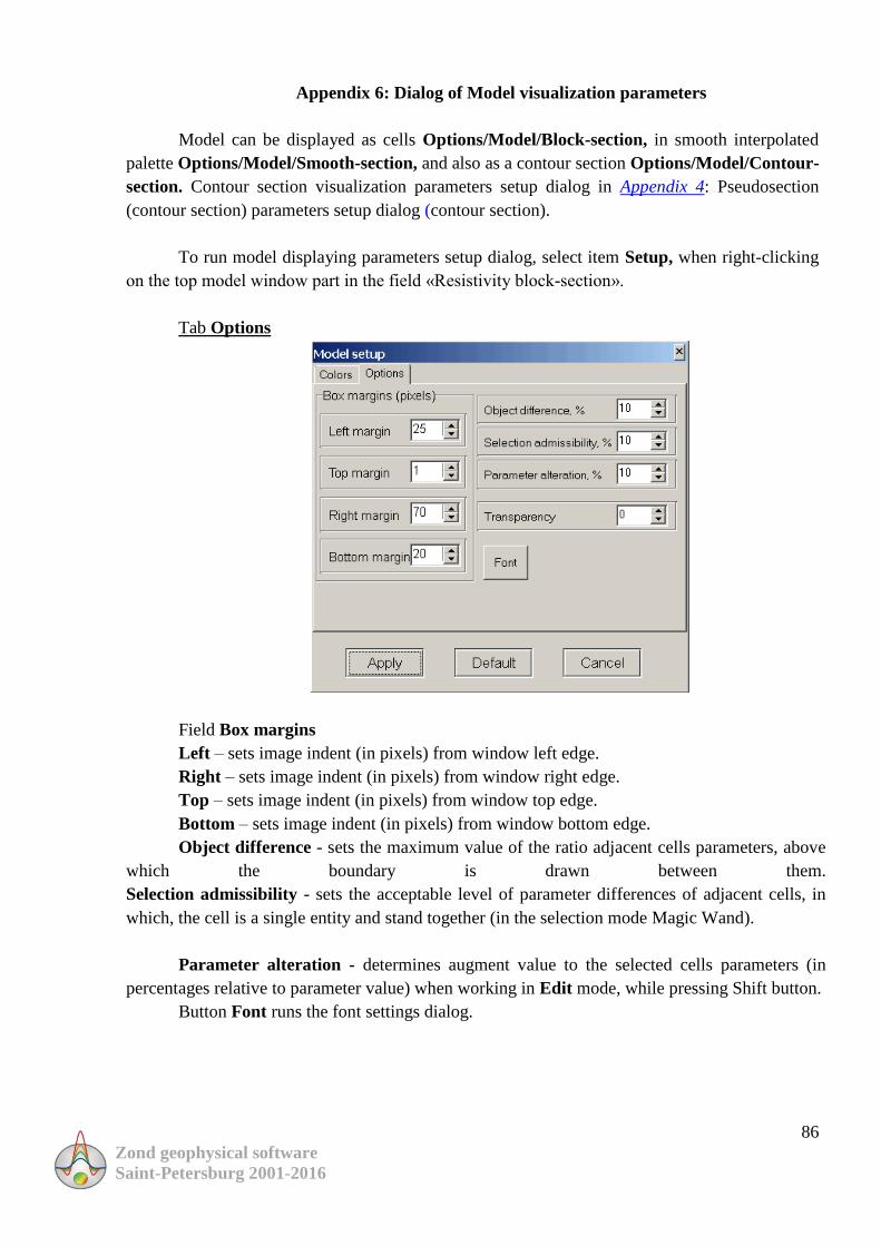
86



Appendix 6: Dialog of Model visualization parameters

Model can be displayed as cells Options/Model/Block-section, in smooth interpolated

palette Options/Model/Smooth-section, and also as a contour section Options/Model/Contour-

section. Contour section visualization parameters setup dialog in Appendix 4: Pseudosection

(contour section) parameters setup dialog (contour section).

To run model displaying parameters setup dialog, select item Setup, when right-clicking

on the top model window part in the field «Resistivity block-section».

Tab Options

Field Box margins

Left – sets image indent (in pixels) from window left edge.

Right – sets image indent (in pixels) from window right edge.

Top – sets image indent (in pixels) from window top edge.

Bottom – sets image indent (in pixels) from window bottom edge.

Object difference - sets the maximum value of the ratio adjacent cells parameters, above

which the boundary is drawn between them.

Selection admissibility - sets the acceptable level of parameter differences of adjacent cells, in

which, the cell is a single entity and stand together (in the selection mode Magic Wand).

Parameter alteration - determines augment value to the selected cells parameters (in

percentages relative to parameter value) when working in Edit mode, while pressing Shift button.

Button Font runs the font settings dialog.

87



Tab Colors

Palette - sets the color palette:

The palette can be changed, edited, loaded from a file and saved to file with extension *.clr of

Surfer program.

A convenient tool for selecting the maximum and minimum resistivity values is to specify

them using vertical line positions on the resistivity distribution diagram

(Options/Extra/Model&Data histograms).

Field Other

Body border - allows specifying the boundaries color between adjacent cells, if the

difference degree between them is greater than the set one in the option Parameter alteration.

Grid - sets the grid color.

Selection - sets the label color of the selected cell.

Fixed - sets the label color of the fixed cell.

When editing the model as a contour section the setting dialog is similar to pseudosection

parameters setup dialog (Appendix 4: Pseudosection (contour section) parameters setup dialog).

88



Appendix 7: Pseudosection points editor

Editor allows adjusting pseudosection points, electrode position points and their labels. It

is called by right-clicking with SHIFT button pressing on the point.

Tab Format contains interface settings of pseudosection points and electrode position

points. Tab Marks contains signatures settings. These tabs options are described in details in

Appendix 1: graphics set editor.

Appendix 8. Zdconvert program

Zdconvert program serves to create data files for «ZONDMT1D» and «ZONDMT2D»

programs. Table files in txt or dat format which contain frequency, apparent resistivity, and

impedance phase values are necessary to work with the program. The program has three main

windows (fig. A8). List of sounding sites organized as 5-column table is located in the top right

window: Filename – name of source file, Name – assigned name of the station, Used –

include/exclude station data from new file, pozX – distance from the beginning of profile, pozZ –

elevation of measuring point. The former four columns can be edited.

Observed and smoothed curves of apparent resistivity and phase impedance for selected

station are displayed in the left window of the program. Double left click on necessary axis to

run setup dialog of vertical and horizontal axes.

Main program window with three tabs is located in the bottom right corner.

Tab Files:

Field Data files – contains information about directory that contains source data files and

name of resultant ZondMT1D file.

Input DIR – open directory that contains source data files.

89



Output File – set outbound ZondMT1D (*.mdf) file name.

Filed File type – specifies type of outbound file.

Create Zond1D file – create file of 1D inversion program ZondMT1D.

Create XYZ file – this option is used to export data of parameters (apparent resistivity

and phase impedance) distribution on certain frequency that is set in pop-up window. Additional

column pozY, that can be edited, also appears in data window. It allows receiving areal

parameters distribution.

Depending on selected type of outbound file Create Zond1D or Create XYZ button is

located in the bottom area. After pressing this button corresponding file is created in the directory

where Zdconvert program is saved.

Window of auxiliary program Zdconvert

Tab Converter:

Field Range dividing – specifies type of filling outbound curves with points. Automatic

filling (Automatic) or filling in logarithmic frequency mesh (Equal log-step) is possible.

Include boundary frequencies – sets whether end points are included to outbound

curves or not.

Smoothing – enable/disable smoothing curve options.

Frequencies number – number of points on resultant curve.

Press Process button to accept all specifications.

Three bottom fields serve to integrate two files of 1D inversion program for different

polarizations in one 2D inversion file. Select 1D inversion files which correspond to TM and TE

90



modes in two left windows, specify file name in the right window, and press button . 2D

inversion file (*.m2d) will be created in the directory that contains source 1D inversion files.

Tab Config is used for source files parameters setup. Specify number of columns in data

file, number of column with apparent resistivity, impedance phases and frequency values in

Columns number, Rho column index, Phase column index и Frequency column index fields

respectively.

Specify extensions of source data files (e.g., dat or txt) in the right window.

Turn log_rho option on if source data file contains decimal logarithm values of apparent

resistivity.

Use button to open list of *.prd files. This list should be saved in the folder with initial

data and should contain three columns: PozX, PozZ and File name (distance along profile,

excess and file name respectively).

Button is used to create list from already opened files.

Window Step sets step along profile between stakes in kilometers.

Program for two-dimensional interpretation of data ...

Documents

Transcript of Program for two-dimensional interpretation of data ...