Prognostics-based Scheduling to Extend a Platform Useful Life...

Prognostics-based Scheduling to Extend a PlatformUseful Life under Service Constraint

Stéphane Chrétien*, Nathalie Herr**, Jean-Marc Nicod** and ChristopheVarnier**

* Laboratoire de Mathématiques de Besançon (LMB) – UFC** FEMTO-ST Institute – Besançon – France

July 2nd, 2014

1. Context and State of the art

Production scheduling• Heterogeneous, independant, parallel machines• Production based on a customer demand

Maintenance

Operating conditions⇒ Consideration of many running profiles

Prognostics and Health Management (PHM)

9th Scheduling for Large Scale Systems Workshop, Lyon 2014 – [email protected] 2 / 20



Maintenance• Wear and tear on machines• Only one global maintenance allowed

⇒ Production horizon maximization before maintenance






Maintenance⇒ Production horizon maximization








⇒ Taking real wear and tear into consideration (and not average life)

Prognostics and Health Management (PHM)• Machine monitoring• Remaining Useful Life (RUL) value depending on past and future usage



Prognostics and Health Management (PHM)• Maintenance scheduling based on actual health state

◊ Haddad et al.: maintenance optimization under availability requirement[“A real options optimization model to meet availability requirements for offshore wind turbines”, MFPT,

Virginia, 2011]

◊ Vieira et al.: maintenance scheduling based on health limits[“New variable health threshold based on the life observed for improving the scheduled maintenance of a

wind turbine”, 2nd IFAC Workshop on Advanced Maintenance Engineering, 2012]

• Maintenance scheduling and mission reconfiguration

◊ Balaban et al.: rover maintenance optimization and mission durationextension[“A mobile robot testbed for prognostic-enabled autonomous decision making”, Annual Conference of the

Prognostics and Health Management Society, 2011]



Operating conditions• Variable-speed machines: control of time used by jobs on machines

◊ Trick: single and multiple machine variable-speed scheduling[“Scheduling multiple variable-speed machines”, Operations Research, 1994, 42, p.234-248]

◊ Dietl et al.: derating of cutting tools by reducing the cutting speed[“An operating strategy for high-availability multi-station transfer lines”, Int. J. of Automation and Computing,

2006, 2, p.125 - 130]

• Voltage/Frequency scaling

◊ Kimura et al.: energy consumption reducing without impactingperformance[“Empirical study on reducing energy of parallel programs using slack reclamation by dvfs in a power-scalable

high performance cluster”, IEEE Int. Conf. on Cluster Computing, Barcelona, 2006]

◊ Semeraro et al.: microprocessor’s performance and energy efficiencymaximization[“Energy-efficient processor design using multiple clock domains with dynamic voltage and frequency

scaling”, HPCA, Cambridge, 2002]






⇒ Taking real wear and tear into consideration (and not average life)

Prognostics and Health Management (PHM)⇒ Use of prognostics results: RUL

⇒ Prognostics-based scheduling


Outline

1. State of the art

2. Scheduling with running profiles in a discrete throughput domainProblem statementComplexity resultsOptimal approachSub-optimal resolutionResultsSummary

3. Scheduling with running profiles in a continuous throughput domainProblem statementConvex optimizationSummary

4. Conclusion


2.1. Problem statement

Problem data• m independant machines (Mj )• n running profiles (Ni )• PHM monitoring→ (ρi,j ,RULi,j )




ρ0,j

ρ1,j

ρ2,j 100%

use

timeRUL0,j RUL1,j RUL2,j

reliability

End Of Life




Constraints• No RUL overrun• Mission fulfillment: constant demand in terms of throughput (σ)

Objective• To fulfill total throughput requirements as long as possible

MAXK(σ | ρi,j | RULi,j )

• Time discretization (T = K ×∆T , 1 ≤ k ≤ K )



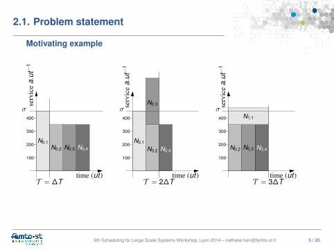
Motivating example

M3

N0,3 = (ρ0,3 = 350W ,RUL0,3 = 1u.t .)N1,3 = (ρ1,3 = 100W ,RUL1,3 = 2u.t .)

M2N0,2 = (ρ0,2 = 350W ,RUL0,2 = 1u.t .)N1,2 = (ρ1,2 = 100W ,RUL1,2 = 2u.t .)

M1N0,1 = (ρ0,1 = 450W ,RUL0,1 = 1u.t .)N1,1 = (ρ1,1 = 125W ,RUL1,1 = 3u.t .)

M4

N0,4 = (ρ0,4 = 350W ,RUL0,4 = 1u.t .)N1,4 = (ρ1,4 = 100W ,RUL1,4 = 2u.t .)



Motivating example

300

200

100

400

N0,1N0,4N0,3

serv

ice

a.ut−

1

T = ∆Ttime (ut)

σ

N0,2

300

200

100

400

N0,1

N0,4

N0,3

N0,2

serv

ice

a.ut−

1

T = 2∆Ttime (ut)

σ

300

200

100

400

N0,2 N0,4N0,3

serv

ice

a.ut−

1

T = 3∆T

σ

time (ut)

N1,1


2.2. Complexity results

Complexity map

Homogeneous machines Heterogeneous machines

ρi,j = ρ ρi,j = ρj

MAXK(σ | ρ |RULj ) MAXK(σ | ρj |RULj )1 running profile

⇒ polynomial ⇒ NP-complete

ρi,j = ρi ρi,j = ρi,j

MAXK(σ | ρi |RULi,j ) MAXK(σ | ρi,j |RULi,j )n running profiles

⇒? ⇒ NP-complete


2.3. Optimal approach

Binary Integer Linear Program (BILP)ai,j,k = 1 if machine Mj is used with running profile Ni during period k ,

0 otherwise

∀k , ∀j,n−1∑i=0

ai,j,k ≤ 1 (machines)

∀j,n−1∑i=0

∑Kk=1 ai,j,k ×∆T

RULi,j≤ 1 (RUL)

∀k ,m∑

j=1

n−1∑i=0

ai,j,k × ρi,j ≥ σ (service)

• Binary search to find maximal value of k

⇒ Limited to small instances: ≈ 5 machines, 2 running profiles, 20 timeperiods


2.4. Sub-optimal resolution

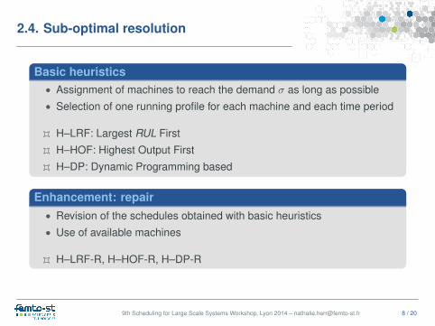
Basic heuristics• Assignment of machines to reach the demand σ as long as possible• Selection of one running profile for each machine and each time period

◊ H–LRF: Largest RUL First

◊ H–HOF: Highest Output First

◊ H–DP: Dynamic Programming based

Enhancement: repair• Revision of the schedules obtained with basic heuristics• Use of available machines

◊ H–LRF-R, H–HOF-R, H–DP-R



• H–DP schedule

K = 4

σ

time

Remaining potential

M1 M1 M1 M1

M2M2M2M2

N0 N0 N0 N0

N0N0N0N0M3 M3 M3 M3N0 N0 N0 N0

serv

ice

• H–DP-R Step 1σ

time

Remaining potential

K = 5

M1 M1 M1 M1M3

M2M2M2M2

M3N0

N0 N0 N0N0

N0N0N0N0N0

M3 M3N0 N0

serv

ice

• H–DP-R Step 2σ

time

Remaining potential

K = 6

M3

M1 M1

M3M2 M2

M2 M2

M3M3M1M1

N0 N0N0 N0

N0 N0

N0N0N0N0N0N0

serv

ice



Basic heuristics• Assignment of machines to reach the demand σ as long as possible• Selection of one running profile for each machine and each time period

◊ H–LRF: Largest RUL First

◊ H–HOF: Highest Output First

◊ H–DP: Dynamic Programming based

Enhancement: repair• Revision of the schedules obtained with basic heuristics• Use of available machines

◊ H–LRF-R, H–HOF-R, H–DP-R


2.5. Results

Simulations

• Validation of heuristics on random problem instances• Consideration of an increasing output Qi,j = ρi,j ×RULi,j with ρ such that:

Q0,j > Q1,j > . . . > Qn−1,j

with ρ0,j > ρ1,j > . . . > ρn−1,j

and RUL0,j < RUL1,j < . . . < RULn−1,j

• Constant demand σk = σ, with:

σ = α×∑

1≤j≤mρmaxj

with 30% ≤ σ ≤ 90%

• Average value of 20 instances with same parameters values


2.5. Results

Comparison to an upper bound(n=5, m=25)

KMAX =

⌊∑jmax

i(ρi,j × RULi,j ) / σ

⌋

40

50

60

70

80

90

100

30 40 50 60 70 80 90

dis

t-K

MA

X (

%)

Load (%)

H-LRFH-HOF

H-DP


2.5. Results

Comparison to an upper bound(n=5, m=25)

KMAX =

⌊∑jmax

i(ρi,j × RULi,j ) / σ

⌋

40

50

60

70

80

90

100

30 40 50 60 70 80 90

dis

t-K

MA

X (

%)

Load (%)

H-LRFH-HOF

H-DPH-LRF-RH-HOF-R

H-DP-R


2.6. Summary

Adressed problem: maximizing the production horizon under serviceconstraint

• Scheduling using prognostics results (RUL)• Choose of running profiles in a discrete throughput domain• Extension of a platform operational time• Efficient sub-optimal heuristics (6% from upper bound)

[MIM2013], [PHM2014*], [CASE2014]

⇒ Application on wind turbines, cutting tools

Second adressed problem• Choose of running profiles in a continuous throughput domain

⇒ Application on fuel cells

• Continuous use of machines

* Best Paper Award


Outline

1. State of the art

2. Scheduling with running profiles in a discrete throughput domainProblem statementComplexity resultsOptimal approachSub-optimal resolutionResultsSummary

3. Scheduling with running profiles in a continuous throughput domainProblem statementConvex optimizationSummary

4. Conclusion



Problem data• m independant machines (Mj )• Running profiles in a continuous throughput domain

(ρminj ≤ ρj (t) ≤ ρmaxj (t))• PHM monitoring→ (ρj (t),RULj (ρj (t), t))• Constant minimal throughput (ρminj )• Maximal throughput decreasing with time (ρmaxj (t))





ρj

time

ρmaxj (0)

100%

ρnomj 70%

RUL(ρnomj )

20%

ρmaxj (t) = aj t + ρmaxj (0)

ρmaxj (0)

ρminj 10%

RUL(ρminj )





Constraints• No RUL overrun• Mission fulfillment: constant demand in terms of throughput (σ)• Avoid temporary machine shutdowns

Objective• To fulfill total throughput requirements as long as possible

MAXK(σ | ρj (t) | RULj (ρj (t), t))


3.2. Convex optimization – Model

Problem statement Model

• Machine throughput fj(t)= ρj(t) if the machine is used

during the period t,

= 0 otherwise

∀j = 1, . . . ,m and ∀t = 0, . . . , T

• Solution: schedule F =

f1(0)f2(0)

...fm(0)

...f1(T )

...fm(T )


3.2. Convex optimization – Model

Problem statement Model• Continuous running profiles fj(t) = f1,j(t) + f2,j(t)

∀j = 1, . . . ,m and ∀t = 0, . . . , T

• Constant minimal throughput fj(t) ≥ fminj

∀j = 1, . . . ,m and ∀t = 0, . . . , T

• Maximal throughput decreasingwith time

fj(t) ≤ fmaxj(t)∀j = 1, . . . ,m and ∀t = 0, . . . , T

• No RUL overrun∑T

t=0Γ(fj(t)) ≤ 1

∀j = 1, . . . ,m

• Mission fulfillment∑m

j=1fj(t) ≥ σ(t)

∀j = 1, . . . ,m and ∀t = 0, . . . , T


3.2. Convex optimization – Constraints

Model Constraint functions

fj (t) = f1,j (t) + f2,j (t)

fj (t) ≥ fminj

∀j = 1, . . . ,m and ∀t = 0, . . . , T

ψ1,j(F)t = f1,j(t)

ψ2,j(F)t = f2,j(t)∀j = 1, . . . ,m

fj(t) ≤ fmaxj(t)∀j = 1, . . . ,m and ∀t = 0, . . . , T

ψ3,j(F)t = fmaxj(t)− fj(t)∀j = 1, . . . ,m

∑T

t=0Γ(fj(t)) ≤ 1

∀j = 1, . . . ,m

ψ4,j(F)t = 1−T∑

t=0

Γ(fj(t))

∀j = 1, . . . ,m

with Γ(fj (t)) =aj ∆T

fj (t)− fmaxj (0)∑m

j=1fj(t) ≥ σ(t)

∀j = 1, . . . ,m and ∀t = 0, . . . , T

ψ0(F)t =m∑

j=1

fj(t)− σ(t)


3.2. Convex optimization – Scheme

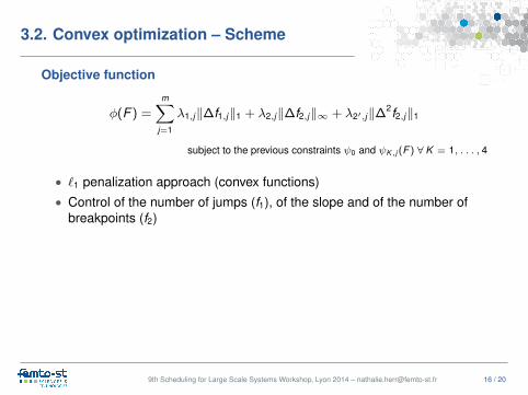
Objective function

φ(F ) =m∑

j=1

λ1,j‖∆f1,j‖1 + λ2,j‖∆f2,j‖∞ + λ2′,j‖∆2f2,j‖1

subject to the previous constraints ψ0 and ψK ,j (F ) ∀K = 1, . . . , 4

• `1 penalization approach (convex functions)• Control of the number of jumps (f1), of the slope and of the number of

breakpoints (f2)


3.2. Convex optimization – Scheme

Objective function

φ(F ) =m∑

j=1

λ1,j‖∆f1,j‖1 + λ2,j‖∆f2,j‖∞ + λ2′,j‖∆2f2,j‖1

subject to the previous constraints ψ0 and ψK ,j (F ) ∀K = 1, . . . , 4

Bregman-proximal method⇒ Minimization of the objective function

⇒ Assures the positivity for each constraint function:ψ0(F ) ≥ 0 and ψK ,j (F ) ≥ 0 ∀K = 1, . . . , 4 and ∀ j = 1, . . . ,m

Lagrange function

L(F , u) = ‖F‖1 + φ(F ) +m∑

j=1

ujψ4,j (F )

such that u ≤ 0, ψ0(F ) ≥ 0 and ψK ,j (F ) ≥ 0 ∀K = 1, . . . , 3


3.2. Convex optimization

Coupled ADMM Bregman-proximal scheme(ADMM: Alternating Direction Method of Multipliers)

Primal step:

F (l+1) = argminF∈R2m(T +1)

(L(F , u(l)) + λ

(Dh(ψ0(F (l)), ψ0(F ))

)+ < V ′(l)

, F − F ′> + < V ′′(l)

, F − F ′′> + < V ′′′(l)

, F − F ′′′>

+ρ

2‖F − F ′‖2

F +ρ

2‖F − F ′′‖2

F +ρ

2‖F − F ′′′‖2

F

)

F ′(l+1) = argminF′∈R2m(T +1)

F=F (l+1)

(λ

( m∑j=1

Dh(ψ1,j (F ′(l)), ψ1,j (F ′))

)+ < V ′(l)

, F − F ′> +

ρ

2‖F − F ′‖2

F

)

F ′′(l+1) = argminF′′∈R2m(T +1)

F=F (l+1)

(λ

( m∑j=1

Dh(ψ2,j (F ′′(l)), ψ2,j (F ′′))

)+ < V ′′(l)

, F − F ′′> +

ρ

2‖F − F ′′‖2

F

)

F ′′′(l+1) = argminF′′′∈R2m(T +1)

F=F (l+1)

(λ

( m∑j=1

Dh(ψ3,j (F ′′′(l)), ψ3,j (F ′′′))

)+ < V ′′′(l)

, F − F ′′′> +

ρ

2‖F − F ′′′‖2

F

)




Primal step: F (l+1), F ′(l+1), F ′′(l+1), F ′′′(l+1)

Dual step:

u(l+1) = argmaxu

(L(F (l+1)

, u) + λDh(u(l), u))

V ′(l+1) = V ′(l) + F (l+1) − F ′(l+1)

V ′′(l+1) = V ′′(l) + F (l+1) − F ′′(l+1)

V ′′′(l+1) = V ′′′(l) + F (l+1) − F ′′′(l+1)




Primal step: F (l+1), F ′(l+1), F ′′(l+1), F ′′′(l+1)

Dual step:

u(l+1) = argmaxu

(L(F (l+1)

, u) + λDh(u(l), u))

V ′(l+1) = V ′(l) + F (l+1) − F ′(l+1)

V ′′(l+1) = V ′′(l) + F (l+1) − F ′′(l+1)

V ′′′(l+1) = V ′′′(l) + F (l+1) − F ′′′(l+1)

Work in progress...


3.3. Summary


• Scheduling using prognostics results (RUL)• Choose of running profiles in a continuous throughput domain• Extension of a platform operational time

⇒ Convergence results of the method...

⇒ Experiment results...


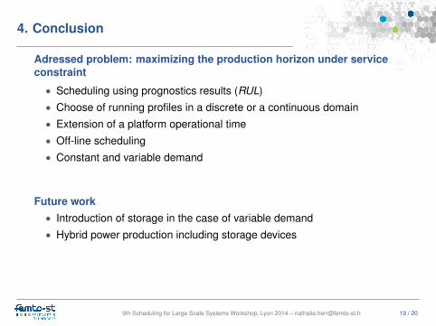
4. Conclusion


• Scheduling using prognostics results (RUL)• Choose of running profiles in a discrete or a continuous domain• Extension of a platform operational time• Off-line scheduling• Constant and variable demand

Future work• Introduction of storage in the case of variable demand• Hybrid power production including storage devices


4. Conclusion

Thank you for your attention

Any questions ?


Prognostics-based Scheduling to Extend a Platform Useful Life...

Documents

Transcript of Prognostics-based Scheduling to Extend a Platform Useful Life...