HAL Id: hal-00798464https://hal.archives-ouvertes.fr/hal-00798464

Submitted on 8 Mar 2013

HAL is a multi-disciplinary open accessarchive for the deposit and dissemination of sci-entific research documents, whether they are pub-lished or not. The documents may come fromteaching and research institutions in France orabroad, or from public or private research centers.

L’archive ouverte pluridisciplinaire HAL, estdestinée au dépôt et à la diffusion de documentsscientifiques de niveau recherche, publiés ou non,émanant des établissements d’enseignement et derecherche français ou étrangers, des laboratoirespublics ou privés.

Feature Evaluation for Effective Bearing Prognostics.Fatih Camci, Kamal Medjaher, Noureddine Zerhouni, Patrick Nectoux

To cite this version:Fatih Camci, Kamal Medjaher, Noureddine Zerhouni, Patrick Nectoux. Feature Evaluation for Ef-fective Bearing Prognostics.. Quality and Reliability Engineering International, Wiley, 2012, pp.1-15.�10.1002/qre.1396�. �hal-00798464�

Feature Evaluation for Effective Bearing Prognostics

F. Camcia, K. Medjaher

b, N. Zerhouni

b, P. Nectoux

b

a IVHM Centre School of Applied Sciences Cranfield University, UK

b FEMTO-ST Institute, UMR CNRS 6174-UFC/ENSMM/UTBM, France

Abstract – Rolling element bearing failure is one of the foremost causes of

breakdown in rotating machinery. It is not uncommon to replace a defected/used

bearing with a new one that has shorter remaining useful life than the defected

one. Thus, prognostics of bearing plays critical role for increased availability and

reduced cost. Effective prognostics highly depend on the quality of the extracted

features. Diagnostics is basically a classification problem, whereas the

prognostics is the process of forecasting the future health states. The quality of the

features for classification has been studied thoroughly. However, evaluation of the

quality of features for prognostics is a relatively new problem. This paper presents

an evaluation method for the goodness of the features for prognostics and presents

results on bearings run until failure in a lab environment.

I. Introduction

Rolling element bearing failure is one of the foremost causes of breakdown in rotating

machinery [1]. Bearing faults account for the 40% of motor faults according to the

research conducted by Electric Power Research Institute (EPRI) [2]. Turbine engine

bearing failures are the leading cause of class-A mechanical failures (loss of aircraft)

[3]. Even one aircraft saved with prognostics would pay its development cost [4].

Bearing faults can be categorized as follows: 1) outer bearing race defects 2) inner

bearing race defect 3) ball defects 4) cage (train) defect. There are also faults such as

imbalance, misalignment, looseness, and debris contamination, which include high

randomness related to environment and human error. Bearings are typically designed to

have a life greater than the subsystem they are in. Failure initiation in bearings includes

high randomness especially for failures related to debris contamination or mishandling.

Currently, defects of size much smaller than 6.25 mm2, which is commonly considered

as a fatal failure size by industry standard [5], can be detected using diagnostics

methods. However, failure detection forces machinery to shut down that causes

tremendous time, productivity and capital loss. In addition, it is not uncommon to

replace a defected/used bearing with a new one that has shorter remaining useful life

than the defected one. For example, remaining useful life of a bearing with a newly

detected defect may be substantially more than its L10 life, which is the life of 90%

bearing population survival [1], [5]. Thus, identification of the most convenient time of

maintenance after failure detection without reducing the safety requirements is crucial,

which is possible with prognostics capability. Thus, bearing prognostics is very critical

for effective operation & management.

Each failure type causes a distinct signature in the vibration frequency [2] and vibration

analysis is considered as the most reliable method in bearing failure detection [6]-[9].

However, it is often difficult to extract the failure signature due to the noise in the data

especially in early stages of the failure [10]-[12]. Thus, several other sensor types such

as current [13] and angular speed [14] have been used for bearing fault detection.

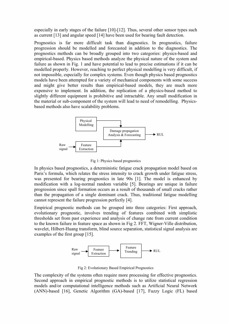
Prognostics is far more difficult task than diagnostics. In prognostics, failure

progression should be modelled and forecasted in addition to the diagnostics. The

prognostics methods can be broadly grouped into two categories: physics-based and

empirical-based. Physics based methods analyze the physical nature of the system and

failure as shown in Fig. 1 and have potential to lead to precise estimations if it can be

modelled properly. However, reaching to perfect physical modelling is very difficult, if

not impossible, especially for complex systems. Even though physics based prognostics

models have been attempted for a variety of mechanical components with some success

and might give better results than empirical-based models, they are much more

expensive to implement. In addition, the replication of a physics-based method to

slightly different equipment is prohibitive and intractable. Any small modification in

the material or sub-component of the system will lead to need of remodelling. Physics-

based methods also have scalability problems.

Fig 1: Physics based prognostics

In physics based prognostics, a deterministic fatigue crack propagation model based on

Paris’s formula, which relates the stress intensity to crack growth under fatigue stress,

was presented for bearing prognostics in late 90s [1]. The model is enhanced by

modification with a log-normal random variable [5]. Bearings are unique in failure

progression since spall formation occurs as a result of thousands of small cracks rather

than the propagation of a single dominant crack. Thus, traditional fatigue modelling

cannot represent the failure progression perfectly [4].

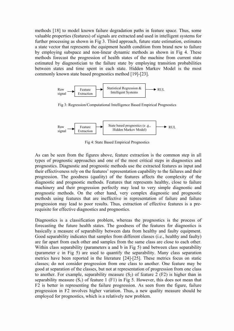
Empirical prognostic methods can be grouped into three categories: First approach,

evolutionary prognostic, involves trending of features combined with simplistic

thresholds set from past experience and analysis of change rate from current condition

to the known failure in feature space as shown in Fig 2. FFT, Wigner-Ville distribution,

wavelet, Hilbert-Huang transform, blind source separation, statistical signal analysis are

examples of the first group [15].

Fig 2: Evolutionary Based Empirical Prognostics

The complexity of the systems often require more processing for effective prognostics.

Second approach in empirical prognostic methods is to utilize statistical regression

models and/or computational intelligence methods such as Artificial Neural Network

(ANN)-based [16], Genetic Algorithm (GA)-based [17], Fuzzy Logic (FL) based

Feature

Trending Feature

Extraction

Raw

signal RUL

Physical

Modelling

Feature

Extraction

Raw

signal

Damage propagation

Analysis & Forecasting RUL

methods [18] to model known failure degradation paths in feature space. Thus, some

valuable properties (features) of signals are extracted and used in intelligent systems for

further processing as shown in Fig 3. Third approach, future state estimation, estimates

a state vector that represents the equipment health condition from brand new to failure

by employing subspace and non-linear dynamic methods as shown in Fig 4. These

methods forecast the progression of health states of the machine from current state

estimated by diagnostician to the failure state by employing transition probabilities

between states and time spent in each state. Hidden Markov Model is the most

commonly known state based prognostics method [19]-[23].

Fig 3: Regression/Computational Intelligence Based Empirical Prognostics

Fig 4: State Based Empirical Prognostics

As can be seen from the figures above, feature extraction is the common step in all

types of prognostic approaches and one of the most critical steps in diagnostics and

prognostics. Diagnostic and prognostic methods use the extracted features as input and

their effectiveness rely on the features’ representation capability to the failures and their

progression. The goodness (quality) of the features affects the complexity of the

diagnostic and prognostic methods. Features that represents healthy, close to failure

machinery and their progression perfectly may lead to very simple diagnostic and

prognostic methods. On the other hand, very complex diagnostic and prognostic

methods using features that are ineffective in representation of failure and failure

progression may lead to poor results. Thus, extraction of effective features is a pre-

requisite for effective diagnostics and prognostics.

Diagnostics is a classification problem, whereas the prognostics is the process of

forecasting the future health states. The goodness of the features for diagnostics is

basically a measure of separability between data from healthy and faulty equipment.

Good separability indicates that samples from different classes (i.e., healthy and faulty)

are far apart from each other and samples from the same class are close to each other.

Within class separability (parameters a and b in Fig 5) and between class separability

(parameter c in Fig 5) are used to quantify the separability. Many class separation

metrics have been reported in the literature [24]-[25]. These metrics focus on static

classes; do not consider progression from one class to another. One feature may be

good at separation of the classes, but not at representation of progression from one class

to another. For example, separability measure (S2) of feature 2 (F2) is higher than in

separability measure (S1) of feature 1 (F1) in Fig 5. However, this does not mean that

F2 is better in representing the failure progression. As seen from the figure, failure

progression in F2 involves higher variation. Thus, a new quality measure should be

employed for prognostics, which is a relatively new problem.

Feature

Extraction

Raw

signal

State based prognostics (e .g.,

Hidden Markov Model) RUL

Feature

Extraction

Raw

signal

Statistical Regression &

Intelligent Systems RUL

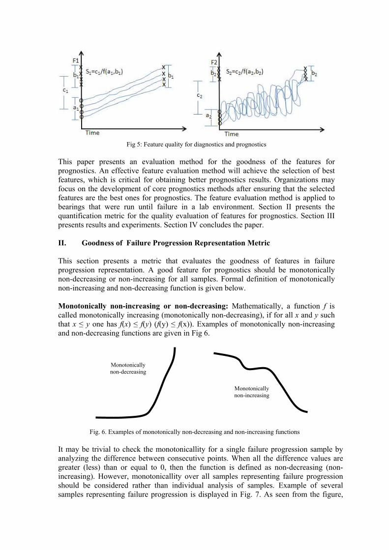
Fig 5: Feature quality for diagnostics and prognostics

This paper presents an evaluation method for the goodness of the features for

prognostics. An effective feature evaluation method will achieve the selection of best

features, which is critical for obtaining better prognostics results. Organizations may

focus on the development of core prognostics methods after ensuring that the selected

features are the best ones for prognostics. The feature evaluation method is applied to

bearings that were run until failure in a lab environment. Section II presents the

quantification metric for the quality evaluation of features for prognostics. Section III

presents results and experiments. Section IV concludes the paper.

II. Goodness of Failure Progression Representation Metric

This section presents a metric that evaluates the goodness of features in failure

progression representation. A good feature for prognostics should be monotonically

non-decreasing or non-increasing for all samples. Formal definition of monotonically

non-increasing and non-decreasing function is given below.

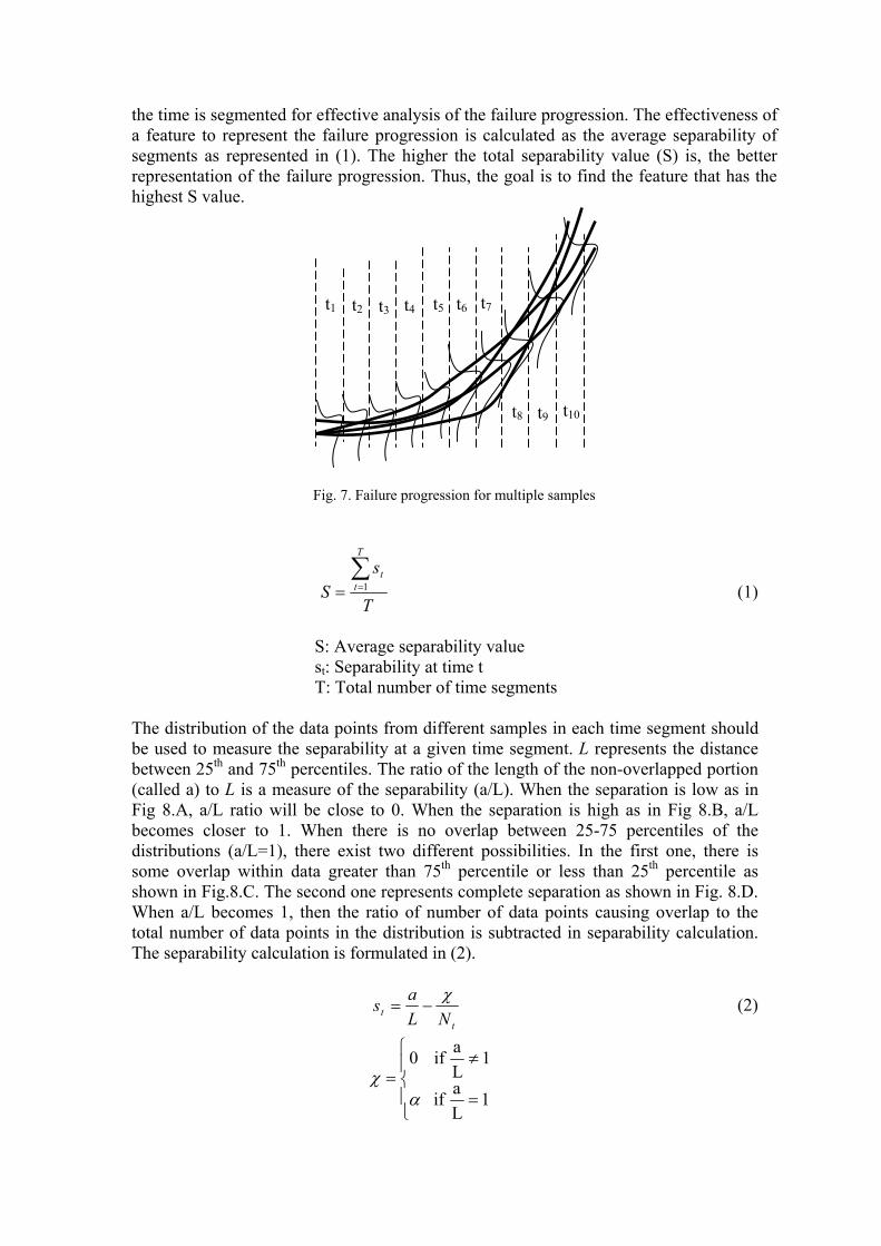
Monotonically non-increasing or non-decreasing: Mathematically, a function f is

called monotonically increasing (monotonically non-decreasing), if for all x and y such

that x ≤ y one has f(x) ≤ f(y) (f(y) ≤ f(x)). Examples of monotonically non-increasing

and non-decreasing functions are given in Fig 6.

Fig. 6. Examples of monotonically non-decreasing and non-increasing functions

It may be trivial to check the monotonicallity for a single failure progression sample by

analyzing the difference between consecutive points. When all the difference values are

greater (less) than or equal to 0, then the function is defined as non-decreasing (non-

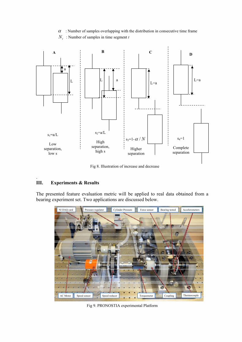
increasing). However, monotonicallity over all samples representing failure progression

should be considered rather than individual analysis of samples. Example of several

samples representing failure progression is displayed in Fig. 7. As seen from the figure,

Monotonically

non-decreasing

Monotonically

non-increasing

the time is segmented for effective analysis of the failure progression. The effectiveness of

a feature to represent the failure progression is calculated as the average separability of

segments as represented in (1). The higher the total separability value (S) is, the better

representation of the failure progression. Thus, the goal is to find the feature that has the

highest S value.

Fig. 7. Failure progression for multiple samples

T

s

S

T

t

t∑== 1 (1)

S: Average separability value

st: Separability at time t

T: Total number of time segments

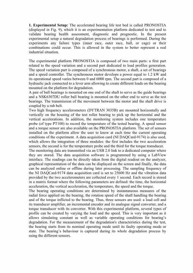
The distribution of the data points from different samples in each time segment should

be used to measure the separability at a given time segment. L represents the distance

between 25th

and 75th

percentiles. The ratio of the length of the non-overlapped portion

(called a) to L is a measure of the separability (a/L). When the separation is low as in

Fig 8.A, a/L ratio will be close to 0. When the separation is high as in Fig 8.B, a/L

becomes closer to 1. When there is no overlap between 25-75 percentiles of the

distributions (a/L=1), there exist two different possibilities. In the first one, there is

some overlap within data greater than 75th

percentile or less than 25th

percentile as

shown in Fig.8.C. The second one represents complete separation as shown in Fig. 8.D.

When a/L becomes 1, then the ratio of number of data points causing overlap to the

total number of data points in the distribution is subtracted in separability calculation.

The separability calculation is formulated in (2).

t

tNL

as

χ−= (2)

⎪⎩⎪⎨⎧

=≠=

1L

a if

1L

a if 0

αχ

t1 t2 t3 t4 t5 t6 t7

t8 t9 t10

α : Number of samples overlapping with the distribution in consecutive time frame

tN : Number of samples in time segment t

Fig 8. Illustration of increase and decrease

.

III. Experiments & Results

The presented feature evaluation metric will be applied to real data obtained from a

bearing experiment set. Two applications are discussed below.

Fig 9. PRONOSTIA experimental Platform

a

L aL L=a

L=a

s1=a/L

Low

separation,

low s

s2=a/L

High

separation,

high s

s3=1- N/α

Higher

separation

s4=1

Complete

separation

A B CD

Bearing tested Accelerometers

TorquemeterSpeed sensorAC Motor

NI DAQ card Pressure regulator

Speed reducer

Force sensor

ThermocoupleCoupling

Cylinder Pressure Bearing tested Accelerometers

TorquemeterSpeed sensorAC Motor

NI DAQ card Pressure regulator

Speed reducer

Force sensor

ThermocoupleCoupling

Cylinder Pressure

1. Experimental Setup: The accelerated bearing life test bed is called PRONOSTIA

(displayed in Fig. 9), which it is an experimentation platform dedicated to test and to

validate bearing health assessment, diagnostic and prognostic. In the present

experimental setup a natural degradation process of bearings is performed. During the

experiments any failure types (inner race, outer race, ball, or cage) or their

combinations could occur. This is allowed in the system to better represent a real

industrial situation.

The experimental platform PRONOSTIA is composed of two main parts: a first part

related to the speed variation and a second part dedicated to load profiles generation.

The speed variation part is composed of a synchronous motor, a shaft, a set of bearings

and a speed controller. The synchronous motor develops a power equal to 1.2 kW and

its operational speed varies between 0 and 6000 rpm. The second part is composed of a

hydraulic jack connected to a lever arm allowing to create different loads on the bearing

mounted on the platform for degradation.

A pair of ball bearings is mounted on one end of the shaft to serve as the guide bearings

and a NSK6307DU roller ball bearing is mounted on the other end to serve as the test

bearings. The transmission of the movement between the motor and the shaft drive is

coupled by a rub belt.

Two high frequency accelerometers (DYTRAN 3035B) are mounted horizontally and

vertically on the housing of the test roller bearing to pick up the horizontal and the

vertical accelerations. In addition, the monitoring system includes one temperature

probe (of type PT100) to record the temperature of the tested bearing. A speed sensor

and a torque sensor are also available on the PRONOSTIA platform. The set of sensors

installed on the platform allow the user to know at each time the current operating

conditions of the experiment. A data acquisition card (NI DAQCard-9174) is also used,

which allows the integration of three modules: the first includes the two acceleration

sensors, the second is for the temperature probe and the third for the torque transducer.

The monitoring data are transmitted via an USB 2.0 link to a dedicated computer where

they are stored. The data acquisition software is programmed by using a LabView

interface. The readings can be directly taken from the digital readout on the analyzer,

graphical representation of the data can be displayed on the screen and finally, the data

can be analyzed online or offline during later processing. The sampling frequency of

the NI DAQCard-9174 data acquisition card is set to 25600 Hz and the vibration data

provided by the two accelerometers are collected every 1 second. Each record is stored

in a matrix format where the following parameters are defined: the time, the horizontal

acceleration, the vertical acceleration, the temperature, the speed and the torque.

The bearing operating conditions are determined by instantaneous measures of the

radial force applied on the bearing, the rotation speed of the shaft handling the bearing

and of the torque inflicted to the bearing. Thus, three sensors are used: a load cell and

its transducer amplifier, an incremental encoder and its analogue signal converter, and a

torque transducer with its converter. With this experimental platform, several types of

profile can be created by varying the load and the speed. This is very important as it

allows simulating constant as well as variable operating conditions for bearing’s

degradation. For the measurement of the degradation's characteristics during the test,

the bearing starts from its nominal operating mode until its faulty operating mode or

state. The bearing’s behaviour is captured during its whole degradation process by

using the different sensors.

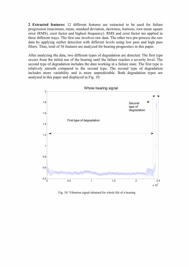
2 Extracted features: 12 different features are extracted to be used for failure

progression (maximum, mean, standard deviation, skewness, kurtosis, root mean square

error (RMS), crest factor and highest frequency). RMS and crest factor are applied in

three different ways. The first one involves raw data. The other two pre-process the raw

data by applying outlier detection with different levels using low pass and high pass

filters. Thus, total of 36 features are analyzed for bearing prognostics in this paper.

After analyzing the data, two different types of degradation are detected. The first type

occurs from the initial use of the bearing until the failure reaches a severity level. The

second type of degradation includes the data working in a failure state. The first type is

relatively smooth compared to the second type. The second type of degradation

includes more variability and is more unpredictable. Both degradation types are

analyzed in this paper and displayed in Fig. 10.

0 0.5 1 1.5 2 2.5

x 104

0.4

0.6

0.8

1

1.2

1.4

1.6

1.8

2

Whole bearing signal

First type of degradation

Secondtype ofdegradation

Fig. 10: Vibration signal obtained for whole life of a bearing

Max Mean Stdev Skew Kurtosis rms CF rms1 rms2 CF1 CF2 freq0

1

2

3

4

5

6

7

Max Mean Stdev Skew Kurtosis rms CF rms1 rms2 CF1 CF2 freq0

1

2

3

4

5

6

7

All data

Highpass

Lowpass

All data

Highpass

Lowpass

Vibration Signal 1

Vibration Signal 2

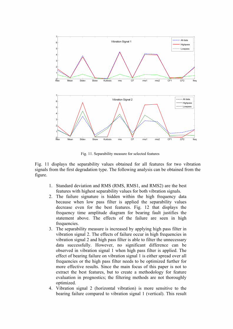
Fig. 11. Separability measure for selected features

Fig. 11 displays the separability values obtained for all features for two vibration

signals from the first degradation type. The following analysis can be obtained from the

figure.

1. Standard deviation and RMS (RMS, RMS1, and RMS2) are the best

features with highest separability values for both vibration signals.

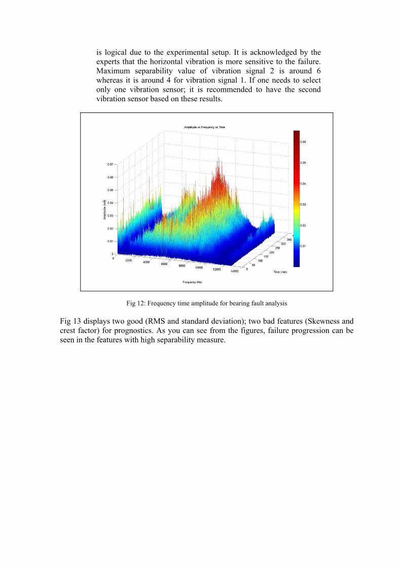
2. The failure signature is hidden within the high frequency data

because when low pass filter is applied the separability values

decrease even for the best features. Fig. 12 that displays the

frequency time amplitude diagram for bearing fault justifies the

statement above. The effects of the failure are seen in high

frequencies.

3. The separability measure is increased by applying high pass filter in

vibration signal 2. The effects of failure occur in high frequencies in

vibration signal 2 and high pass filter is able to filter the unnecessary

data successfully. However, no significant difference can be

observed in vibration signal 1 when high pass filter is applied. The

effect of bearing failure on vibration signal 1 is either spread over all

frequencies or the high pass filter needs to be optimized further for

more effective results. Since the main focus of this paper is not to

extract the best features, but to create a methodology for feature

evaluation in prognostics; the filtering methods are not thoroughly

optimized.

4. Vibration signal 2 (horizontal vibration) is more sensitive to the

bearing failure compared to vibration signal 1 (vertical). This result

is logical due to the experimental setup. It is acknowledged by the

experts that the horizontal vibration is more sensitive to the failure.

Maximum separability value of vibration signal 2 is around 6

whereas it is around 4 for vibration signal 1. If one needs to select

only one vibration sensor; it is recommended to have the second

vibration sensor based on these results.

Fig 12: Frequency time amplitude for bearing fault analysis

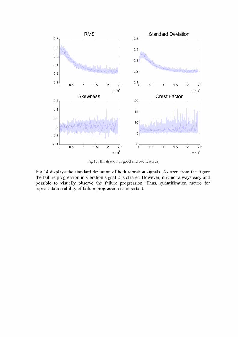
Fig 13 displays two good (RMS and standard deviation); two bad features (Skewness and

crest factor) for prognostics. As you can see from the figures, failure progression can be

seen in the features with high separability measure.

0 0.5 1 1.5 2 2.5

x 104

0.2

0.3

0.4

0.5

0.6

0.7

RMS

0 0.5 1 1.5 2 2.5

x 104

0.1

0.2

0.3

0.4

0.5

Standard Deviation

0 0.5 1 1.5 2 2.5

x 104

-0.4

-0.2

0

0.2

0.4

0.6

Skewness

0 0.5 1 1.5 2 2.5

x 104

0

5

10

15

20

Crest Factor

Fig 13: Illustration of good and bad features

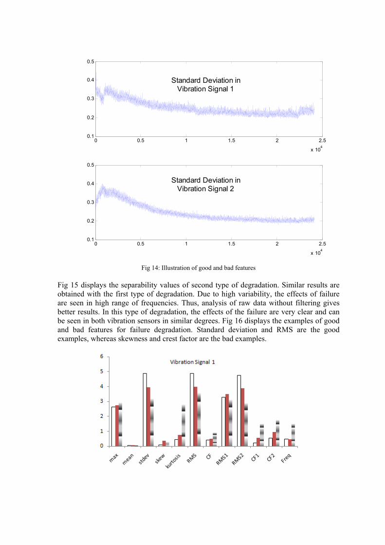
Fig 14 displays the standard deviation of both vibration signals. As seen from the figure

the failure progression in vibration signal 2 is clearer. However, it is not always easy and

possible to visually observe the failure progression. Thus, quantification metric for

representation ability of failure progression is important.

0 0.5 1 1.5 2 2.5

x 104

0.1

0.2

0.3

0.4

0.5

Standard Deviation inVibration Signal 1

0 0.5 1 1.5 2 2.5

x 104

0.1

0.2

0.3

0.4

0.5

Standard Deviation inVibration Signal 2

Fig 14: Illustration of good and bad features

Fig 15 displays the separability values of second type of degradation. Similar results are

obtained with the first type of degradation. Due to high variability, the effects of failure

are seen in high range of frequencies. Thus, analysis of raw data without filtering gives

better results. In this type of degradation, the effects of the failure are very clear and can

be seen in both vibration sensors in similar degrees. Fig 16 displays the examples of good

and bad features for failure degradation. Standard deviation and RMS are the good

examples, whereas skewness and crest factor are the bad examples.

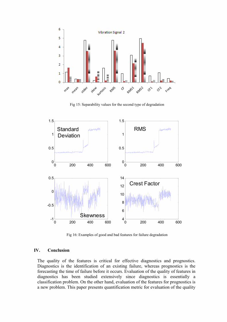
Fig 15: Separability values for the second type of degradation

0 200 400 6000

0.5

1

1.5

Standard Deviation

0 200 400 6000

0.5

1

1.5

RMS

0 200 400 600-1

-0.5

0

0.5

Skewness0 200 400 600

4

6

8

10

12

14

Crest Factor

Fig 16: Examples of good and bad features for failure degradation

IV. Conclusion

The quality of the features is critical for effective diagnostics and prognostics.

Diagnostics is the identification of an existing failure, whereas prognostics is the

forecasting the time of failure before it occurs. Evaluation of the quality of features in

diagnostics has been studied extensively since diagnostics is essentially a

classification problem. On the other hand, evaluation of the features for prognostics is

a new problem. This paper presents quantification metric for evaluation of the quality

of features. The presented metric is applied to features extracted from bearing

vibration data collected. Bearings were run until failure in a lab environment. 12

features are extracted for raw, high pass filtered, and low pass filtered data. The

results obtained from the presented metric are very promising and justified with

analysis of the bearing failure analysis.

References

[1] Li Y., Billington S., Zhang C., Kurfess T., Danyluk S., Liang S., “Adaptive

Prognostics For Rolling Element Bearing Condition”, Mechanical Systems and

Signal Processing 13(1), 103-113, 1999

[2] Enzo C.C. L., Ngan H. W., “Detection of Motor Bearing Outer Raceway Defect

by Wavelet Packet Transformed Motor Current Signature Analysis”, IEEE

Transactions on Instruments and Measurement, 59(10), 2683-2690, 2010

[3] Wade Richard A. “A Need-focused Approach to Air Force Engine Health

Management Research” Health Management Research IEEE Aerospace

Conference Big Sky, Montana, 2005

[4] Marble S., Morton B.P., “Predicting the Remaining Useful Life of Propulsion

System Bearings”, Proceedings of the 2006 IEEE Aerospace Conference, Big

Sky, MT, USA, 2006

[5] Li Y., Kurfess T. R., Liang S. Y., “Stochastic Prognostics For Rolling Element

Bearing”, Mechanical Systems and Signal Processing, 14(5), 747-762, 2000

[6] Zhang B., Sconyers C., Orchard M., Patrick R., Vachtsevanos G., “Fault

Progression Modeling: An Application to Bearing Diagnosis and Prognosis”,

Proceedings of American Control Conference, MD USA, 2010

[7] Davaney M., Eren L., “Detecting Motor Bearing Faults”, IEEE Instrumentation &

Measurement Magazine, 30-50, 2004

[8] McFadden P.D., Smith J. D., “Vibration monitoring of rolling element bearings

by the high frequency resonance technique – a review”, Tribology International,

17, 3-10, 1984

[9] Tandon N., Choudhury A., “A review of vibration and acoustic measurement

methods for the detection of defects in rolling element bearings”, Tribology

International, 32, 469-480, 1999

[10] Su W., Wang F., Zhu H., Zhang Z., Guo Z., “Rolling element bearing faults

diagnosis based on optimal Morlet Wavelet filter and autocorrelation

enhancement”, Mechanical Systems and Signal Processing, 24, 1458-1472, 2010

[11] Bozchalooi I. S., Liang M., “A joint resonance frequency estimation and in-band

noise reduction method for enhancing the detectability of bearing fault signals”,

Mechanical Systems and Signal Processing 22, 915-933, 2008

[12] He W., Jiang Z. N., Feng K., “Bearing fault detection based on optimal wavelet

filter and sparse code shrinkage”, Measurement, 42, 1092-1102, 2009

[13] Immovilli F., Bellini A., Rubini R., Tassoni C., “Diagnosis of Bearing Faults in

Induction Machines by Vibration or Current Signals: A Critical Comparison”,

IEEE Transactions on Industry Applications, 46(4), 1350-1359, 2010

[14] Renaudin L., Bonnardot F., Musy O., Doray J. B., Remond D., “Natural roller

bearing fault detection by angular measurement of true instantaneous angular

speed”, Mechanical Systems and Signal Processing 24, 1998-2011, 2010

[15] Rafiee J., Rafiee M. A., Tse P. W., “Application of mother wavelet functions for

automatic gear and bearing fault diagnosis”, Expert Systems with Applications,

37, 4568-4579, 2010

[16] Paya B.A., Esat I. I., Badi M. N. M., “Artificial neural network based fault

diagnosis for rotating machinery using wavelet transforms as a pre-processor”,

Mechanical Systems and Signal Processing, 11(5), 751-765

[17] Samanta B., Gear fault detection using artificial neural network & support vector

machine with genetic algorithms, Mechanical Systems and Signal Processing,

18(3), 625-644, 2004

[18] Saravanan N., Cholairajan S., Ramachandran K. I., “Vibration-based fault

diagnosis of spur bevel gear box using fuzzy technique”, Expert systems with

applications, 35(3), 1351-1366

[19] Ocak H., Loparo K. A., Discenzo F. M., “Online Tracking of bearing wear using

wavelet packet decomposition and probabilistic modelling: A method for bearing

prognostics”, Journal of Sound and Vibration, 302, 951-961, 2007

[20] R. B. Chinnam, P. Baruah, Autonomous diagnostics and prognostics in machining

processes through competitive learning-driven HMM-based clustering,

International Journal of Production Research, 47 (23), 2009, 6739 – 6758.

[21] M. Dong, D. He, A segmental hidden semi-Markov model (HSMM) -based

diagnostics and prognostics framework and methodology, Mechanical Systems

and Signal Processing, 21, 2007, 2248-2266

[22] Camci, R. B. Chinnam., "Health-State Estimation and Prognostics in Machining

Processes", IEEE Transactions on Automation Science and Engineering, 7(3),

2010, 581-597

[23] P. Baruah and R. B. Chinnam, HMMs for diagnostics and prognostics in

machining processes, “International Journal of Production Research”, 43(6),

2005, 1275–1293

[24] Calinski R. B. and Harabasz J., A Dendrite Method for Cluster Analysis, Comm.

in Statistics, 3, 1974, 1-27

[25] Eker O. F., Camci F, Guclu A., Yilboga H., Sevkli M., Baskan S.,"A Simple

State- based Prognostic Model for Railway Turnout Systems", IEEE Transactions

on Industrial Electronics, Vol. 58, No. 5, May 2011, 1718-1726