BEARING PROGNOSTICS USING NEURAL NETWORK ...ABSTRACT Bearing Prognostics using Neural Network under...

BEARING PROGNOSTICS USING NEURALNETWORK UNDER TIME VARYING CONDITIONS

MUHAMMAD ADNAN KHAN

A THESIS

IN

THE CONCORDIA INSTITUTE

FOR

INFORMATION SYSTEMS ENGINEERING

PRESENTED IN PARTIAL FULFILLMENT OF THE REQUIREMENTS

FOR THE DEGREE OF MASTER OF APPLIED SCIENCE (QUALITY SYSTEM

ENGINEERING) AT CONCORDIA UNIVERSITY

MONTREAL, QUEBEC, CANADA

AUGUST 2010

© MUHAMMAD ADNAN KHAN, 2010

1*1 Library and ArchivesCanada

Published HeritageBranch

395 Wellington StreetOttawa ON K1A 0N4Canada

Bibliothèque etArchives Canada

Direction duPatrimoine de l'édition

395, rue WellingtonOttawa ON K1A 0N4Canada

Your file Votre référenceISBN: 978-0-494-7 1 004-3Our file Notre référenceISBN: 978-0-494-71004-3

NOTICE: AVIS:

The author has granted a non-exclusive license allowing Library andArchives Canada to reproduce,publish, archive, preserve, conserve,communicate to the public bytelecommunication or on the Internet,loan, distribute and sell thesesworldwide, for commercial or non-commercial purposes, in microform,paper, electronic and/or any otherformats.

L'auteur a accordé une licence non exclusivepermettant à la Bibliothèque et ArchivesCanada de reproduire, publier, archiver,sauvegarder, conserver, transmettre au publicpar télécommunication ou par l'Internet, prêter,distribuer et vendre des thèses partout dans lemonde, à des fins commerciales ou autres, sursupport microforme, papier, électronique et/ouautres formats.

The author retains copyrightownership and moral rights in thisthesis. Neither the thesis norsubstantial extracts from it may beprinted or otherwise reproducedwithout the author's permission.

L'auteur conserve la propriété du droit d'auteuret des droits moraux qui protège cette thèse. Nila thèse ni des extraits substantiels de celle-cine doivent être imprimés ou autrementreproduits sans son autorisation.

In compliance with the CanadianPrivacy Act some supporting formsmay have been removed from thisthesis.

Conformément à la loi canadienne sur laprotection de la vie privée, quelquesformulaires secondaires ont été enlevés decette thèse.

While these forms may be includedin the document page count, theirremoval does not represent any lossof content from the thesis.

Bien que ces formulaires aient inclus dansla pagination, il n'y aura aucun contenumanquant.

1+1

Canada

CONCORDIA UNIVERSITY

School of Graduate Studies

This is to certify that the thesis prepared

By: Muhammad Adnan Khan

Entitled: Bearing Prognostics using Neural Network under Time Varying Conditions

and submitted in partial fulfillment of the requirements for the degree of

Master of Applied Science in Quality System Engineering

complies with the regulations of this University and meets the accepted standards with

respect to originality and quality.

Signed by the final examining committee:

___________________________________________________________Chair

___________________________________________________________Examiner

___________________________________________________________Examiner

___________________________________________________________Supervisor

Approved

Chair of Department or Graduate Program Director

_________20

Dr. Robin A.L. Drew, Dean

Faculty of Engineering and Computer Science

ABSTRACT

Bearing Prognostics using Neural Network under TimeVarying Conditions

MUHAMMAD ADNAN KHAN

Condition based maintenance (CBM) aims to schedule maintenance activities based on

condition monitoring data in order to lower the overall maintenance costs and prevent

unexpected failures.

Effective CBM can lead to reduced downtime, less inventory, reduced maintenance costs,

reliable operation and safety of entire system. The key challenge in achieving effective

CBM is the accurate prediction of equipment future health condition and thus the

remaining useful life. Existing prognostics methods mainly focus on constant loading

conditions. However, in many applications, such as some wind turbine, transmission and

engine applications, the load that the equipment is subject to changes over time. It is

critical to incorporate the changing load in order to produce more accurate prognostics

methods. This research is focused on the bearing prognostics, which are key mechanical

components in rotary machines, supporting the entire load imposed on machines. Failure

of these components can stop the operation due to machine down time, thus resulting in

financial losses, which are much higher than the cost ofbearing.

iii

In this thesis, an artificial neural network (ANN) based method is proposed for equipment

health condition prediction under time varying conditions. The proposed method can be

applied to bearing as well as other components under condition monitoring. In the

proposed ANN model, in addition to using the age and condition monitoring

measurement values as an inputs, a new input neuron is introduced to incorporate the

varying loading condition. The output of the ANN model is accumulated life percentage,

based on which the remaining useful life can be calculated once the ANN is trained. Two

sets of simulated degradation data under time varying load are used to demonstrate the

effectiveness of the proposed ANN method, and the results show that fairly accurate

prediction can be achieved using the proposed method.

The other key contribution of this thesis is the experiment validation of the proposed

ANN prediction method. The Bearing Prognostics Simulator, after extensive adjustment

and tuning, is used to perform bearing run-to-failure test under different loading

conditions. Vibration signals are collected using the data acquisition system and the

Labview software. The root mean square (RMS) measurement of the vibration signals is

used as the condition monitoring input for the validation of the proposed ANN prediction

method. Two bearing failure histories are used to train the ANN model and test its

prediction performance. The results demonstrate the effectiveness of the proposed

method in dealing with real-world condition monitoring data for health condition

prediction. The proposed model can greatly benefit industry as well as academia in

condition based maintenance of rotary machines.

iv

Acknowledgments

I am extremely thankful to all peoples who support me during entire thesis work.

First of all, I am deeply thankful to professor, Dr Zhigang (Will) Tian, who is my supervisor

during this research. His encouragement, guidance and support made my task easy and

interesting. He enriched my academic knowledge in this field by sharing valuable knowledge

all the time. He gives me the opportunity to work on real equipments and facilitate me during

my research work, and build a confidence to proceed further in field of System Engineering

Reliability and Maintenance Optimization.

I would like to thank all the Concordia Institute of Information System Engineering (CIISE)

faculty, and people for their support, and providing me the opportunity to take several

courses, during my study period, through which I have gained a lot of knowledge and

exposure that will surely help me in my career.

I would also like to thank and appreciate my research lab members, for their support and help

during experiments.

Last but not the least , I want to thank my family, my mother who prays for me all the time,

my wife for supporting me during my thesis work, and my two lovely kids.

?

Table of Contents

List of Figures ?

List of Tables , xii

Acronyms xiii

1. Introduction 1

1.1. Background 1

1.2. Condition Based Maintenance 2

1.3. Research Motivation 4

1.4. Research Contribution 5

1.5. Thesis Organization 6

2. Literature Review on Bearing Condition Monitoring 7

2.1. Bearing Diagnostics 7

2.1.1. Application of Neural Network for Fault Diagnostics 10

2.1.2. Application of Other Artificial Intelligence Techniques for Diagnostics 14

2.2. Bearing Prognostics 15

2.2.1. Physics Based Prognostics 16

vi

2.2.2. Data Driven Prognostics 17

2.3. Prognostics under Time Variant Conditions 21

3. Data Analysis and Feature Extraction 23

3.1. Time Domain Analysis 24

3.1.1. Root Mean Square Value (RMS) 25

3.1.2. Kurtosis 26

3.1.3. Peak Value 27

3.1.4. Crest Factor 27

3.2. Frequency Domain Analysis 28

3.3. Spectral Analysis with Fast Fourier Transform 29

3.4. Neural Network 30

3.5. Ball Bearings 34

3.6. Bearing Health Parameters for Prognostics 35

3.6.1. Vibration Analysis 35

3.6.2. Causes of Vibration in Bearings 36

4. Neural Network Model for RUL Prediction 38

4.1. Remaining Useful Life Prediction 38

vii

4.2. The Artificial Neural Network Model for RUL Prediction 40

4.2.1 The FeedForward ANN Model 40

4.2.1.1 Transfer Function 45

4.3. Neural Network Training 46

4.3.1. The Neural Network Training Algorithm 46

4.3.2. The Neural Network Validation 47

4.3.2.1. Generation of Simulated Data 48

4.3.2.2. ANN Model Prediction Results for the First Simulation Data Set 49

4.3.2.3. ANN Model Prediction Results for the Second Simulation Data 52

4.4. Summary 54

5. Experiments Setup and Validation of ANN Model 56

5.1. Bearing Prognostics Simulator 56

5.1.1. Load 59

5.1.2. Test Bearings 60

5.2. Data Acquisition and Signal Processing 61

5.2.1. Vibration measuring Sensor 63

5.2.2. Data Acquisition unit 63

viii

5.2.3. Signal Processing Software 64

5.2.4. Sampling 65

5.3. Validation of the Proposed ANN Prediction Approach Using the Experiment Data 66

5.3.1. The First Experiment 67

5.3.2. Second Experiment 69

5.4. Prediction results with Proposed Neural Network Model 70

6. Conclusions and Future Work 73

6.1. Conclusions 73

6.2. Future Work 74

Bibliography 76

IX

List of Figures

Figure 1: CBM process steps 3

Figure 2: Basic structure of neural network with one input, hidden and output layer 32

Figure 3: Ball Bearing 34

Figure 4: Remaining Useful Life Prediction Procedure 39

Figure 5: Architecture of first FFNN model for prognostics of rolling element bearing . 41

Figure 6: Architecture of modified FFNN mode for prognostics of bearing 44

Figure 7: Failure data generated at sigma level of 0.5 at 450 threshold value 50

Figure 8: Predicted life of first simulation 51

Figure 9: Failure data generated at sigma level of 0.9 at 700 threshold value 53

Figure 10: Predicted life of Second simulation 54

Figure 11: Bearing Prognostics simulator 57

Figure 12: Ball Bearing accelerated life failure test 58

Figure 13: Failed ball bearing after test 59

Figure 14: KOYO 62052 Ball Bearing used in the research 60

Figure 15: Proposed approach for bearing prognostics 62

Figure 16: Vibration Sensor 63

?

Figure 17: Data Acquisition unit 64

Figure 1 8 : Vibration amplitude data collection for Prognostics test 65

Figure 19: RMS values of first experiment at 2500 lbs of load 68

Figure 20: RMS values of second experiment at 3000 lbs of load 69

Figure 2 1 : Predicted life of time varying data with neural network model 71

Xl

List of Tables

Table 1: Data Points 66

Table 2: RMS Calculation 67

XIl

Acronyms

CBM Condition Based Maintenance

ANN Artificial Neural Network

FFNN FeedForward Neural Network

RMS Root Mean Square

ALT Accelerated Life Testing

AI Artificial Intelligence

HFRT High Frequency Resonance Technique

MLP Multi Layer Perceptron

RBF Radial Basis Function

SOM Self Organizing Map

GA Genetic Algorithm

SVM Support Vector Machines

RPROP Resilient Back Propagation Algorithm

PPRL Progression-Based Prediction of remaining

IRLS Improved Redundant Lining Scheme

AE Acoustic Emission

DWNN Dynamic Wavelet Neural Network

XlIl

AR Auto Regression Model

ADT Accelerated Degraded Testing

MSE Mean Square Error

XlV

Chapter 1

Introduction

The main objective of this research is to build a prognostic model for bearing under time

varying conditions. Bearings are often subjected to different operating conditions, like

variation in load, temperature, pressure and speed. Less effort has been made in this area,

and normally prognostic work has been done with assumption of no change in working

parameters of bearings. In this work, data generated through accelerated life failure tests

of bearings, under time varying conditions, are used to predict remaining useful life of

bearings.

1.1. Background

Prognosis is the art of presentation of the remaining useful operational life of

component. This can be achieved through analysis of present working condition of

existing systems, through condition monitoring data. The benefit of accurate prognosis

include reduce downtime, less inventory, reduced maintenance costs, reliable operation

and safety of entire system.

Bearings are considered to be a fundamental type of mechanical components. Their safe

and reliable operation is necessary for the operation of whole equipments. Therefore,

manufacturers and system operators always look forward to developing and

implementing condition based maintenance plan, for these components in order to check1

their existing health condition and predict remaining useful life. Unscheduled

maintenance of the equipments, especially due to bearing failure, is an economical

burden for organizations. Losses due to no production, spare wages for workers, or some

times over time payments in order to meet schedule consignments, are much higher than

the cost of bearings.

1.2. Condition Based Maintenance

Condition Based Maintenance (CBM) techniques are approaches for performing

maintenance activities during the operational activities of components subject to their

working conditions, irrespective of the time frame, or accumulation of certain cycles or

hours. It is a type of preventive maintenance. This is a dynamic approach to achieve

production without unnecessary down time. Jardine et al (2006) have given a detail

review on CBM for rotating machinery implementing diagnostics and prognosis. CBM

provides a maintenance process and decision making maintenance schedule by using the

information collected through condition monitoring. It captures the multiple degraded

states of equipments during operation before they get failed. This health monitoring

information can be used for the prediction of optimal maintenance plan that can have

capability to prevent equipment breakdown and minimize total operation and

maintenance costs. Tian et al. (2009) proposed a model for CBM to avoid unnecessary

maintenance tasks by taking maintenance actions only when there are significant

impended failures seen. CBM program is consisted of two approaches, diagnostics and

prognostics. Diagnostics is a fault detection method. If fault occurs and properly detected2

in time, maintenance operations can be effectively done. Diagnostic activities are related

to fault detection, isolation and identification that are to detect a fault, isolate the

defective area, and identify the nature and extent of fault. A prognostic is a prediction of

future health condition of components.

CBM program comprised of three steps: Data acquisition, data processing and

maintenance decision making, as shown in Figure 1 . In data acquisition, operational data

of equipments are collected through sensors. Data processing is the transformation of raw

data into useful information for analysis and feature extraction. Maintenance decision

making is the last step in which all the information are transformed for effective

maintenance policies required to be taken (Jardine et al., 2006).

Data Acquisition Data Processing Maintenance Decision

Making

Figure 1 : CBM process steps

3

1.3. Research Motivation

Modern era is time of competition in terms of reputation, financial growth and survival

for organizations. Every industry wants to have realistic, prolific and dependable

maintenance plan for their entire production. Maintenance of the equipments is vital in

terms of steady operation. Now a day's industries are looking for cost effective

maintenance practices, in order to optimize their maintenance plan. They want to know

the exact threshold figure for their equipments failure, so that necessary actions can be

taken at correct and scheduled time. This practice also benefits the safety for both

humans and equipments and asset availability.

This research focuses on prognostics of bearings under time varying condition. Bearings

are fundamental components of rotary machines. They support the entire load imposed on

machines. If these components get failed, the operation of whole equipment can be

stopped. As they are located in central position of rotating parts, access to them is only

available after stripping the components most of the times.

Remaining useful life (RUL) prediction of bearings under time varying load condition is

itself a challenge as a research work. The existing RUL prediction work is limited to

fixed operating conditions (e.g., pressure, temperature, humidity, rotating speed, and

load). However, in many applications, such as some wind turbine, transmission and

engine applications, the load that the equipment is subject to changes over time. It is

critical to incorporate the changing load in order to produce more accurate prognosticsmethods

4

1.4. Research Contribution

In this thesis, an artificial neural network (ANN) based method is proposed for equipment

health condition prediction under time varying conditions. The proposed method can be



measurement values as inputs, a new input neuron is introduced to incorporate the

varying loading condition. The output of the ANN model is life percentage, based on

which the remaining useful life can be calculated once the ANN is trained. Two sets of

simulated degradation data under time varying load are used to demonstrate the











method in dealing with real-world condition monitoring data for health condition5



1.5. Thesis Organization

The rest of the Thesis is organized as follows:

• In Chapter 2, a detailed literature review is given on bearings and rotary

machines condition monitoring methods. In the last part, some previous work on

RUL prediction under time varying operating conditions is also discussed.

• In chapter 3, we discuss data analysis and feature extraction techniques, like time

domain and frequency domain analysis, basic theory of artificial neural network,

bearings and vibration analysis, and parameter used in this research to collect

bearing operating characteristics for RUL prediction.

• In Chapter 4, we have discussed in details, our proposed neural network approach

for RUL prediction, and validation with simulated data.

• In Chapter 5, experimental setup, data acquisition method and validation of

proposed model are presented, to demonstrate the capability of new method.

• Finally in Chapter 6, we draw conclusions from our research and set out our

future tasks for ongoing research.

6

Chapter 2

Literature Review on Bearing Condition Monitoring

Bearings are considered to be as a fundamental part of mechanical equipments, due to the

widespread application of rolling element bearings, and it is necessary to effectively

monitor their health condition for safe, reliable and cost effective operations. This

literature review is comprised of previous research work on diagnosis and prognosis of

bearings. Diagnostic research work is discussed, along with artificial intelligence

techniques. Two different methods for prognosis, that is, physics based and data driven

methods, are briefly discussed with previous work. In the last section of this literature

review, remaining useful life of components under time varying condition is also

discussed.

2.1. Bearing Diagnostics

Bearings play an important role for the integrity of machines as they are imposed to the

most severe working condition. Despite the fact they are not expensive in comparison

with the whole cost of equipments, their failure can interrupt the production in a plant,

causing unscheduled downtime and production losses. The subject of rolling bearing

diagnostics has been studied over past three decades. With the rapid increase in

technology and increased in manufacturing of equipments, the need of fault detection in

bearings, specifically in industries, has been realized, so that any impended fault if occurs

can be rectified without disruption to entire plant production. The main objective of7

bearing diagnostics is to isolate and identify the different types of defects that occurred in

bearings during operation. It is accomplished with the help of technology, developed

through physical and statistical means, which involve measuring and processing of

defects induced in bearings for any reason.

The most common methods in bearing diagnostics, for the detection of anomalies for

feature extraction, are time domain and frequency domain analysis of raw signals of

bearings, mainly in form of vibration and acoustic emissions through sensors. In time

domain analysis, some statistical features like root-mean-square (RMS), peak, kurtosis,

crest factor, impulse factor, shape factor, and clearance factor of vibration or acoustic

emission signals, are often used for analysis of data, collected from accelerometers or

acoustic emission sensors mounted on the bearing sleeves or machine casings. Kim et al.

(2007) studied time domain features for condition monitoring of low speed rolling

element bearings for incipient fault detection, by using an acoustic emission (AE) sensor

and an accelerometer.

From statistical point of view, kurtosis value of bearing, which is a fourth order

deviation from mean, is a good representation of bearing condition. Dyer and Stewart

(1978) introduced a statistical parameter, Kurtosis, to measure bearing conditions. Mc-

Fadden and Smith (1984) discussed the high-frequency resonance technique (HFRT) to

evaluate the bearing condition by using anti aliasing filters. E.D. Price et al. (2001)

combined both acoustic emission and vibration data with those from the wear debris

analysis to detect impending failure in bearings.

d

Lee and White (1998) used the impulsive sound and vibration signals and passed these

signals to two stage adaptive line enhancer, one to remove tonal and other to remove

broadband noise from the signals. In addition to this sometimes other associated

components of entire system produces noises which can mingle with bearing vibration

signals causing difficulties in interpretation. Khemili and Chouchane (2005) proposed a

classical approach to clean noisy signal by passing it through filters. Zhang et al (2008)

proposed bearing anomaly detection through envelope signal spectrum, and as the fault

dimension increases it shows a monotonie decrease trend. Early failure indication is

usually detectable at higher frequencies. Therefore, waveform analysis and demodulation

at these frequencies can be performed for time/frequency domain processing. Every time

the defect rolls over the race bearings generate an impulse, and the demodulation process

can be used to detect these impulse events.

Tandon and Choudhary (1997) proposed an analytical model for predicting the vibration

frequencies of rolling bearings and the amplitude of significant frequency components

due to localized defects on outer race. Their model can predict a discrete spectrum having

peaks at the characteristic defect frequencies and their harmonics. Yu et al. (2002) used

high-gain displacement transducers, to measure outer race deflection, resulting as a

defected signal spikes in the time based deflection.

A diagnosis system monitors a finite number of fault modes that are conveniently ranked

and selected according to a Failure Modes, Effects, and Criticality Analysis. These

defects could be the reason of improper installation, misalignment of races, or improper

loading of subsequent assemblies. The failures associated with these defects could appear

9

in form of wear, which is a result of indentation on the raceways on the rolling element,

flaking and smearing due to overloading and inadequate lubrication. Corrosion inclusion

of water between bearing elements leads to pitting of the race ways and the surface of the

bearing and cracks propagation for any reasons (Patii et al, 2008). The dominant mode of

failure of rolling element bearings is spalling of the races or the rolling elements, which

is an initiation of fatigue crack below the surface of the metal and propagates towards the

surface until a piece of metal breaks away to leave a small pit or spall. Marble and

Morton (2006) conducted research on the spall growth trajectory and presented a physics-

based model for bearing condition monitoring.

2.1.1. Application of Neural Network for Fault Diagnostics

Artificial intelligence (AI) is the automation of intelligent behavior, in which an

algorithm is made to assist machines while performing cognitive tasks. With the help of

Artificial Intelligence, intelligent agents are designed, which are actually a system itself

that can perceives their existing environment and can take actions that can maximized

their chances of success. Working principle of artificial intelligence is simply learning,

adaption and storage of knowledge and phenomena, and built in capability to use this

information to solve the problem, and acquire new knowledge through experience.

Several AI techniques are applied for rotary machines diagnostics, and some of the

common are expert system, fuzzy logic, neurofuzzy, and neural network techniques.

Artificial Intelligence techniques are getting popular among the researcher for rotating

machines fault diagnosis. In this literature review some of the techniques and10

contribution will be discussed in general and application of neural network is discussed in

particular as this technique is utilized in this research.

Rolling element bearings are important components, therefore fault diagnosis in the

earlier stages is necessary to prevent further damages in future operational work. Neural

network has so far become very promising for fault diagnosis of bearings. Lots of

research has been conducted for fault detection in bearings, through seeded faults and

also real life industrially used bearings data. Comparison has been made through new

ones for pattern recognition and isolation of defective region. For the analysis of spectral

signatures attained from bearing through sensors, neural networks may be used both as

classifying and clustering systems, for classification purpose. It is important to label the

signature at any instantaneous point to the data taken from machine in order to check the

operational state of machine. The input to the network is a spectrum, or its compressed

version, and the output is the class label. The network is trained to identify an arbitrary

pattern as a member of a state among a set of possible states. Clustering involves the

grouping of patterns according to their internal similarity thus requires no labels. The aim

of clustering is to distribute the set of patterns into classes such that the patterns in each

class have similar statistical and geometrical properties (Israel, et al, 1993).

Several researchers have contributed their work for application of neural network to fault

detection and diagnosis of rolling element bearings. Samanta & Balushi (2003) presented

a procedure for bearing fault diagnostics using time domain features and ANN with fast

training capability. They used time domain features like crest factor, kurtosis and peaks

values after normalization, so that even if the signals changes in magnitude due to change

11

in speed or quality of sensor mounting, the diagnostic results are unaffected as long as the

signal patterns remain unchanged. The training speed of ANN is enhanced after using the

relevant features of the signals characterizing the bearing conditions. Paya et al (1997)

studied both bearing and gear faults. They modeled driveline wear consisting of a number

of rotating parts both separately and simultaneously. The vibration signals acquired from

the driveline were first pre-processed using wavelet transform, and then they used ANNs

to differentiate between each fault and established the exact position of the fault

occurring in the driveline.

Li et al (2000) discussed several bearing vibration features in time and frequency

domain. With the help computer aided software they simulated the data to study and

design the neural network for motor bearing fault diagnosis algorithm, and then they used

actual vibration data collected in real time to perform initial testing and validation of

approach and got effective results in the diagnosis of various motor faults through

appropriate measurement and interpretation of motor bearing vibration signals.

Sreejith et al (2008) used feed-forward neural network with back propagation training

algorithms for fault diagnosis rolling element bearing from vibration data. The time

domain parameters, the Weibull negative log-likelihood values, and the normal negative

log-likelihood values of the time domain vibration signals were used as input features.

The proposed procedure used ANN classifier and required data measured from only one

measurement point. The signal was not pre-processed before the feature extraction. The

algorithm used less number of input features resulting in faster training.

12

Samanta et al (2004) presented a procedure for the diagnosis of bearing condition using

three classifiers, namely, MLP, RBF, and PNN with Genetic Algorithm (GA) based

feature selection from time-domain vibration signals. GA is used to optimize the

classifier parameters and performed successfully for six input parameters of time domain

signals. Another important thing they found regarding neural network is that although the

classification performance of MLP was comparable to that of PNN with six features, the

training time of MLP was much higher than PNN.

Subrahmanyam & Sujatha (1997) used time domain features, like RMS, kurtosis, crest

factor etc, along with frequency domain features of bearing like prime spike region and

high frequency region. They trained two neural networks: a multi-layered feed forward

neural network trained with Error Back Propagation (EBP) algorithm, and an

unsupervised Adaptive Resonance Theory-2 (ART2) based single layered competitive

neural network, by knowing the fact that these neural networks have an edge over

conventional monitoring methods in that they can classify the condition of machine

components, even in the absence of explicit input to output relationships. They got better

performance with EBP, but faster learning time around 100% with ATR2 type of neural

work. Taha & Khusnun (2009) used feed forward back propagation neural network to

detect bearing defect through acoustic emission measurements. They used function

approximation and pattern recognition tasks for anomaly detection in bearings.

13

2.1.2. Application of Other Artificial Intelligence Techniques forDiagnostics

Several other artificial intelligence techniques are gaining importance in the field of

rotary machines diagnostics. Fuzzy logic has shown prolific results in this area of

diagnostic research. Fuzzy logic sets along with statistical data assessment and some pre-

defined sets of standards have proven to be effective, but still a question raised is about

the human subjectivity and adaptive learning of this technique.

Mechefske (1998) investigated the use of basic fuzzy logic techniques as a machinery

fault diagnostic technique. He used fuzzy logic technique to classify frequency spectra

according to likely fault condition. He used membership function domain limits that are

linked to the variability of group spectra of particular type of faults. Fuzzy logic optimum

limits were manually adjusted in this work. Zeng & Wang (1991) used fuzzy logic

technique by fault clustering and fault assignment techniques. From the previous failure

history, they developed fault pattern data base for every type of fault, and established set

of classified clusters, with each cluster representing one type of machine fault. Any kind

of fault signature was passed to this cluster for identification of faults.

Another artificial intelligence technique is expert system. Expert Systems are computer

programs, established through domain knowledge and it utilizes logical operators like

"IF-THEN-ELSE". An expert System is a knowledge based system which stores faults in

its data base, but its limitation is that it cannot figure out new problem, which is not

stored in data base. This non learning capability of expert system is its limitation.

14

Another problem associated with expert system is to obtain knowledge from data base.

Shao & Nezu (1996) applied the principle of expert system to perform monitoring and

diagnosis of bearings. They used recurrence tracing method to minimize accidental

variation in monitoring of bearings. They proposed a degree of credibility of parameter

value variation (DCPV) factor, which can tackle the online variation of intrusive

vibration signals. Jack & Nandi (2000) used six input feature to train a genetic algorithm

for bearing vibration diagnostics and found better accuracy after combining it with ANN.

Samanta (2004) presented a procedure for detection of gear condition using ANN and

support vector machines (SVM) with GA-based feature selection from time-domain

vibration signals. With the help of genetic algorithm he optimized the selection of input

features and the appropriate classifier parameters. He collected different vibration signals

under both normal and light loads, and at low and high sampling rates. He showed that

classification accuracy of SVMs is better than of ANNs, without GA. With GA-based

selection, the performance of both classifiers was comparable at nearly 100%, even with

different load conditions and sampling rates.

2.2. Bearing Prognostics

In present days, reliable estimation of bearings remaining useful life presents the most

challenging aspect in maintenance optimization and catastrophic failure avoidance. So far

the two basic methods deployed for prognostics of rotary machines are Physics Based

and Data Driven.

15

2.2.1. Physics Based Prognostics

A physics-based prognostic involves building of mathematical models based on physical

phenomena of operation of equipments and their internal relationship with each other. As

defects grow within the system and lead towards failure, the failure mechanism and

modes are studied to form physics based models, and that can define defect growth

trajectory, stress/strain relationship of the defects. Using these models, remaining useful

life of the system can be predicted.

Bearing prognostics specifically depends upon the nature of anomalies associated with

different types of bearings and their operational characteristics. Fault projection is tracked

in order to develop prognostics algorithm for RUL prediction. Lybeck et al (2007)

developed a prognostics algorithm for remaining life prediction of bearings and validated

their algorithm, with vibration based diagnostic data. In order to check diagnostic severity

metrics, after feeding this information into proposed model for prognosis for future spall

propagation, they calculated the remaining useful life of bearing. David & Bechhoefer

(2007) developed bearing diagnostics and prognostics tools using health and usage

monitoring system (HUMS) condition indicators. In their model, physical damages of

bearings are correlated with condition indicators for fault diagnosis and prognosis like

nearest neighborhood points from real vibration data.

Janjarasjitt et al (2008) analyzed vibration data corresponding to the operation of test

bearing in an accelerated life experiment, and used partial correlation integral computed16

dimensional exponent. They found that this dimensional component was different for

healthy bearing and bearings close to failure, it tended to increase. They also proposed

computational scheme for bearing condition monitoring using the dimensional exponent

integrated with a surrogate data testing technique. Normally the nature of defect growth

does not follow a linear relationship. Noises in the wide spectrum of a bearing's vibration

signal make this task even more difficult. William et al. (2001) presented a signal

processing method, which attempted to emphasize defect signals over background noise

and built a model for defect growth. Li et al. (1999) presented the formulation of a

bearing prognostic methodology based on the in process adaptation of defect propagation

rate with vibration signal analysis. It utilizes a deterministic defect propagation model

and an adaptive algorithm to fine tune the predicted rate of defect propagation in a real-

time manner.

2.2.2. Data Driven Prognostics

Data driven approaches for bearing prognosis relies on condition monitoring data. Instead

of building physical models, only the current and past state features are used to predict

remaining useful life. During the operation of components, whenever characteristics

features like vibration, acoustic emission, temperature and pressure etc are change, their

sequence of points forms some trajectory and data driven methods use these points to

predict remaining useful life. Some of the measure data driven methods are ANN, hidden

Markov method, auto regressive models etc. Gebrael et al (2005) used the reliability

characteristics of a device's population and real-time sensor information from the

17

functioning device to periodically update the distribution of the bearing's residual life.

They developed a Bayesian approach for updating their estimates of the stochastic

parameters in exponential random-coefficient models and then used these models with

their updated parameters to develop residual-life distributions for partially degraded

components.

Neural network is a widely used tool in the application of data driven prognosis for rotary

machines and equipments. It has shown so far prolific results towards prognosis or

prediction of remaining useful life of bearings. For bearing prognosis research work,

normally there are different ways to collect bearings data. Mostly researchers have used

either vibration or acoustic emission data for most of the research works. The data can be

taken from industrial equipments, through computer aided simulation programs at

different set of conditions, or from lab experiments. This information is then used to train

the neural network on predicting bearing operating times. Bearing sensors data from a

set of validation bearings are then applied to these network models, and thus resulting

predictions are then used to estimate the bearing failure times.

Gebraeel et al (2004) investigated the fatigue process for a group of identical bearings to

calculate variation in bearing life. They performed accelerated life testing on identical

bearings and calculated six harmonic frequencies of bearing which are multiple integers

of defective frequency, and fed the vibration magnitude at these frequencies to train a set

of feed forward back propagation neural network. Their approach was to develop two

classes of models, which were single bearing and cluster of bearing networks relying on

18

data base of degradation signals to predict failure time of a partially degraded bearing at

any time during its service life and got satisfactory results.

Tian & Zuo (2009) proposed an extended recurrent neural network (ERNN) for health

prediction of gearbox based on the vibration data collected form gear box. Fulong et al

(1993) proposed a neural network to implement maximum likelihood method. They

developed bearing likelihood estimation algorithm in real time and demonstrated their

results analytically and through simulation as well. Satish & Sarma (2005) developed a

technique for the detection of bearing condition in induction motors, by combining both

ANN and fuzzy logic, to take the advantages of non linear mapping through ANN and

classification of linguistic and ambiguous information through fuzzy logic. They

developed a Fuzzy BP (Back Propagation) in order to avoid the disadvantages of

individual artificial intelligence techniques.

Huang et al (2007) presented a method for the prediction of a ball bearing's remaining

useful life. Their model was based on self-organizing map (SOM) with unsupervised

learning, and back propagation neural network with supervised learning. To identify the

current operating time of a bearing, they used six vibration features and developed a new

degradation index for performance degradation assessment. Wu et al (2007) developed an

integrated neural-network based decision support system for predictive maintenance of

rotational equipment. They developed a vibration data base and trained a feed forward

back propagation neural network to predict remaining useful life of bearing. They also

constructed a cost matrix and probabilistic model to optimize the expected cost per unit

time.

19

Tian (2009) modified the model proposed by Wu et al (2007), and proposed a new ANN

based model for achieving more accurate RUL prediction. He presented the model that

can take the age and multiple condition monitoring measurement values at discrete

inspection points that is at current point and previous point as the inputs and the life

percentage as the output. He used generalized Weibull-FR function to fit "each condition

monitoring measurement series for a failure history. He trained ANN with these fitted

measurement values got better result than Wu' s method of prediction for remaining

useful life.

Tian et al (2009) used ANN for remaining useful life prediction from suspension

histories rather than only from failure histories of equipment. They realized the potential

of suspension history data that is when equipment is removed from service due to any

reason before it gets failed. For each suspension history they determined optimal

predicted life, which can minimize the validation mean square error. Mahamad et al

(2010) used feed forward neural network with Levenberg-Marquardt training algorithm

for the prediction of RUL of bearings. Their model used time and fitted measurements

with Weibull hazard rates of root mean square (RMS) and kurtosis from its present and

previous points as inputs, and presented the normalized life percentage as an output in

order to minimize the noise of degradation signal from target bearings. Vachtsevanos

(2001) used dynamic wavelet neural network (DWNN) for the prediction of bearing

failures and compared their result with auto regression model (AR) to predict RUL.

20

2.3. Prognostics under Time Variant Conditions

Bearings are normally subjected to time variant conditions imposed through either

environment, or the operating condition of equipment in which they are installed. Current

methods for RUL prediction have considered fixed operating environments, like

temperature, pressure humidity, speed and load. Usually load imposed on bearing are

considered to be stationary. Accurate RUL prediction under time varying conditions is a

challenging and critical work. A recommended solution is to figure out the degradation

characteristics of the unit under operation at several varying conditions, and apply

artificial intelligence techniques, such as neural networks and fuzzy logic to predict RUL

prediction under these conditions. Not much research work has been conducted in this

area, but still research is going on to build the good physical models with capability to

predict RUL under time varying conditions.

Shao & Nezu (2000) proposed a new concept called progression-based prediction of

remaining life (PPRL). For accurate prediction of remaining useful life this model used

different prediction methods to different bearing running stages. They used online

measurements to check level of deterioration during run to failure test and apply PPRL

via a compound model of neural computation. They demonstrated that their model has

the capability to automatically adjust varying environmental factors. Lao & Saleh (1993)

used the frequency features of vibration signal, Power Spectral Density (PSD) and

Discrete Fourier Transform (DFT), to analyze a bearings' vibration characteristics under21

unbalance load in common operation conditions. They developed 2-layer neural network

for RUL prediction of bearings. Their model tracked the fault's feature patterns due to

unbalance faults identified by a set of time based vibration frequency spectrum, contained

in the vibration signal.

Zhang, et al( 2002) conducted a research to predict remaining useful life of bearings, by

accelerated fatigue test under a corrosive environment with the application of inverse

power law. Their theory lies under the fact that RUL prediction model can effectively

work under normal or any other accelerated operating conditions, as long as the stress

level fall within the designed range. They performed bearing life tests under several

corrosion stress levels, and for their model verification, they conducted separated test

under normal conditions for validation purpose. Carey and Koenig (1991) conducted an

accelerated data testing at higher operating temperature levels, to check the reliability of

an integrated logic family under normal operating conditions.

Gebraeel and Pan (2008) have recently developed a prognostic approach for updating the

RUL of a single unit under time-varying environment. They used a linear degradation and

the multivariate normal distribution model to utilize a conjugate prior distribution for

updating the model parameters and RUL prediction. But there proposed approach is still

insufficient to handle complex cases, where degradation stress/strain relationship is

nonlinear. Meeker et al. (1998) presented an approximate maximum likelihood method

for their nonlinear mixed-effects ADT model.

22

Chapter 3

Data Analysis and Feature Extraction

Data analysis is the transformation of raw sensor data into useful information for decision

making. Feature extraction is a procedure of handling raw data in way to reduce curse of

dimensionality, as the data collected is normally consisted of several thousand points.

Therefore in order to classify them, we need suitable methods for transformation and at

the same time, we do not want loose the information available in the data. Several data

analysis techniques are used for feature extraction of bearing defects. Most of the

prominent techniques are time domain, frequency domain, and time-frequency domain

analysis. Time domain analysis mainly comprise of statistical analysis of time varying

data, captured through sensors. While frequency domain analysis is the conversion of

time domain signal into its frequency components for the detection of defective

frequencies. Several techniques are available, already used by researchers. Some of the

prominent and promising techniques are high frequency resonance technique (HFRT),

power spectral density, cepstrum analysis, spectrum analysis, and so on. All these

techniques have their own advantages and disadvantages. Therefore on individual basis

each technique can be considered as independent, rather complementing each other in

several ways. The most common techniques discussed in this chapter are time domain

and frequency domain analysis, spectral analysis with Fourier transform and neural

network based methods.

23

3.1. Time Domain Analysis

Time domain analysis is one the prominent approach for both bearing diagnosis and

prognosis. Some of the basic time domain features are root mean square (RMS), Standard

deviation, Kurtosis value, Crest factor, Clearance factor, Impulse factor and Shape factor

etc.

Sreejith et al (2008) utilized time domain features for their research on bearing

diagnostics. Kim et all( 2007) also used time domain feature while conducting research

on low speed bearings by a low speed fault simulation test rig, specially developed to

simulate common machine faults, with shaft speeds as low as 10 rpm under loading

conditions. The simplest method is to measure the overall RMS level of the bearing

vibration, and compare from previous or pre set values for the health monitoring

condition of bearings.

Tandon & Nakra (1993) studied RMS technique along with other techniques to detect

bearing defects through simulation. Another point of consideration for RMS is that, it

never shows appreciable changes in the early stages of bearing life, therefore some time

another measurement called crest factor is used, and it is the ratio of the peak level of the

input signal to the RMS level. Higher peaks in the time series signal will increase the

crest factor. When defect occurs, it increases the peak level of vibration signal resulted in

short burst of high energy. Therefore crest factor is a good indication of faults when it is

generated.

24

Kurtosis is also a common method for signature analysis. It is the statistical indicator

used in time history data of bearings signatures, to calculate impulsive character of the

signals. It is a fourth statistic moment of the distribution of data from mean. Dyer &

Stewart (1978) initially introduced its application to bearing fault detection. Sawalhi &

Randall (2005) presented an algorithm for the optimization of spectral kurtosis that can

help choose the best filter. In another work they also proposed a pre-whitening method

for power spectral density of signal prior to the application of spectral kurtosis.

Another technique shock pulse method is also used. It measures maximum amplitude of

sensor's resonances in the time domain. The shock pulses are produced due to impacts in

the bearings, which initiate damped oscillations in the sensor at its resonant frequency,

condition of bearings is indicated by measuring the maximum value of the damped

transient pulses. Zhen et al (2008) proposed new approach for improved redundant lifting

scheme (IRLS), by adding the normalization factors in time domain features to avoid

error propagation of decomposition results. Some of the basic time domain features were

briefly given with their mathematical representation.

3.1.1. Root Mean Square Value (RMS)

As described earlier, The RMS is the most common statistical tool to evaluate the overall

performance of bearings vibration level its rapid response detection characteristics makes

it more suitable to use in accelerated failure life testing of bearings. During the

experiment for quick judgment, practically for good bearings initially this indicator

remains steady, and starts increasing gradually and then shows rapid increase in last25

hours of experiments till bearing get failed. The RMS value is given by the following

equation:

Signal (RMS) = J^C(S,.)2 (3-1)Where N is the total number of data points captured during sampling in one history of

entire signal and S¡ is the ith member of data set S. We used the above equation for our

calculation of RMS of the data, captured during failure tests through accelerometer and

we processed them in Matlab.

3.1.2. Kurtosis

Kurtosis is a fourth moment of the distribution and measures the relative peakedness or

flatness of a distribution. We can estimate the sharpness of distribution of vibration data

with the help of this function. Normally, vibration signals of healthy bearings follow

Gaussian distribution. It does not depend upon the load and revolutions. Therefore the

value of the kurtosis is close to three for the vibration signals of healthy bearings. As the

propagation of cracks rises, this will increase the kurtosis value a lot more than three. As

damage becomes severe, kurtosis values starts decreasing practically near three.

Therefore, the extent ofbearing damage may be assessed by examining the distribution of

the kurtosis in selected frequency ranges.

26

Mathematically Kurtosis can be expressed as

Kurtosis=^-¿(^^)4 (3.2)Where N is the total numbers of data points captured during sampling in one history of

entire signal, S¡ is the ith member of data set S , s is the standard deviation, and µ is

the mean of all points in data set S

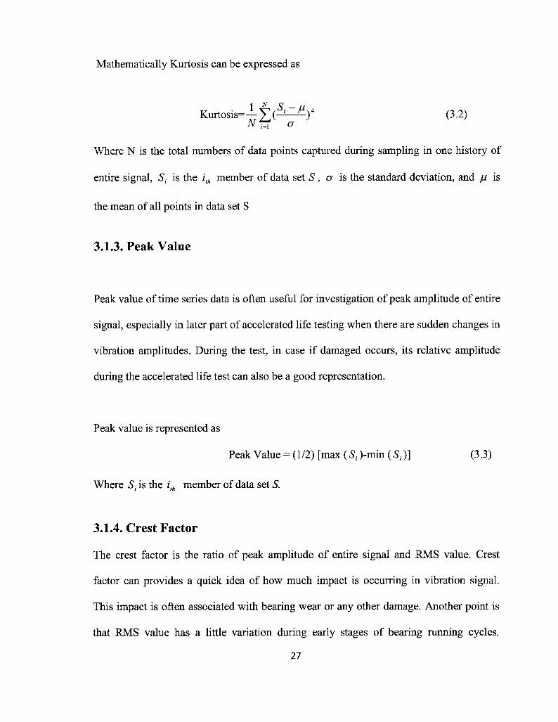
3.1.3. Peak Value

Peak value of time series data is often useful for investigation of peak amplitude of entire

signal, especially in later part of accelerated life testing when there are sudden changes in

vibration amplitudes. During the test, in case if damaged occurs, its relative amplitude

during the accelerated life test can also be a good representation.

Peak value is represented as

Peak Value = (1/2) [max ( S1 )-min ( S, )] (3.3)

Where S¡ is the ith member of data set S.

3.1.4. Crest Factor

The crest factor is the ratio of peak amplitude of entire signal and RMS value. Crest

factor can provides a quick idea of how much impact is occurring in vibration signal.

This impact is often associated with bearing wear or any other damage. Another point is

that RMS value has a little variation during early stages of bearing running cycles.

27

Therefore in case of damages, peak values will increase and eventually crest factor will

increase, which indicates , the running condition of bearing. For normal bearing, its

accepted value is 2 to 6. Values more than 6 can be considered as an indication of

defective bearings.

Mathematically

„. ^ PeakValue ,„ ..Crest Factor= (3.4)RMS

3.2. Frequency Domain Analysis

For bearing fault diagnosis and prognosis, Frequency domain also called Spectral

analysis has become more significant and prolific approach due to its features. In this

technique, characteristics frequencies of rolling element bearing components are

collected in the form of impulses from the wave form of signals. Most prominent

techniques are high frequency resonance technique (HFRT), spectrum analysis, cepstrum

analysis, synchronized averaging, etc.

HFRT is the technique that utilizes envelope detection of bearing signatures. In this

technique, vibration signatures are either attenuated or preamplified, and then these

processed signals are routed to a band pass filter, set for an appropriate carrier frequency.

These filtered signals are then rectified and demodulated to develop the envelope, the

frequencies of this envelop are analyzed through frequency spectrum analyzer. Rolling

element bearing components have their own defective frequencies which appears in this

envelops for any kind fault detection.28

Shiroishi et al (1997) used HFRT along with adaptive line enhancer for fault detection in

bearings. They used two accelerometers and acoustic emission sensors to detect bearing

defects in outer and inner races. Martin and Thorpe (1992) presented the concept of

normalization of the envelope-detected frequency spectra. They compared signal of both

faulty and healthy bearing to give rated numbers, thus ensuring more sensitivity to the

detection of defect frequencies. Ho & Randal (2000) simulated bearing fault signals and

investigated the efficient application of self-adaptive noise cancellation (SANC) in

conjunction with envelope analysis in order to remove discrete frequency masking

signals. They suggested Hilbert transform or either band-pass rectification technique for

combination of these signals. Cepstrum is defined as the spectrum of the logarithmic

power of spectrum. Tandon (1994) used cepstrum along with several time domain

features to detect of different sizes in bearing.

3.3. Spectral Analysis with Fast Fourier Transform

Bearing Vibration signature are captures through mounted sensors or transducers. These

signals are normally captured in time varying conditions or in time domain. Therefore in

order to analyze these signals, it is important to select a proper technique in order to

analyze those signals to conclude the ongoing problem or condition of bearings at the

prevailing stages. Spectral analysis is used to transform a signal from the time domain to

the frequency domain and vice versa. With The application of Fourier Transform

function we can get the spectral content of a periodic function.29

The Fourier transform of function X (t) is given by as follows:

OO

X(J) = jx(t)eiwtdt (3.5)-co

Transformation of X (t) to X (f) is from time to frequency, and the whole transformed

function is the sum of sine and cosine of different frequencies, and w is rotational

component which is equals to 2p?.

FFT or Fast Fourier Transform splits time signals into sub components with amplitude,

a phase, and a frequency. Every associated frequency reflects its characteristics. Its

amplitudes can be useful to work out the problems. Theoretically all waveforms,

irrespective of their complexities can be expressed as sum of sine and cosine waves of

different amplitudes, phase, and frequencies. FFT performs this function by breakdown,

the complex time waveform into components and eliminate time axis, resulting in

demonstration of graph that can represent frequency versus amplitude.

3.4. Neural Network

An artificial neural network (ANN) has now become the more popular for pattern

recognition of mechanical components, especially for rotary machines. Artificial neural

networks map the input data into selected output categories using artificial neurons

similar to biological nervous system. ANN works in a layer pattern, the input layer,

hidden layer, and output layer. Each layer consists of nodes. The lines between the nodes

indicate the flow of information between the nodes. For the feed forward neural

networks, the information flows only from the input to the output. The nodes of the input30

layer are passive, which mean they cannot modify the data. The nodes of the hidden and

output layer are active. The values in a hidden node are multiplied by weights. The

weighted inputs are then added to produce single results. Before leaving the node, this

result is passed through a nonlinear mathematical function called a transfer function. The

active nodes of the output layer combine and modify the data to produce the output

values of the neural network (Sorin, 2001).

Neural networks are designed to classify input patterns in some selected classes or to

create categories that group patterns according to their similarity. They can model

processes and systems from actual data. The neural network is supplied with data and

then "trained" to find the input-output relationship of the process, or system. Neural

networks also have the ability to respond in real time to the changing system state

descriptions provided by continuous inputs. Therefore, when there are lots of inputs or

the system is complex neural network can provide a realistic solution.

Architecture of Neural networks is comprised of simple elements operating in parallel,

similar to biological nervous systems. As in nature, the connections between elements

largely determine the network function. We can train a neural network to perform a

particular function by adjusting the values of the connections (weights) between

elements.

31

Input Parameters

Neurons

Weight

Hidden layer

Output

Input layer Output layer

Figure 2: Basic structure of neural network with one input, hidden and output layer.

The two methods for pattern recognition in neural network training are supervised and

unsupervised learning. A supervised learning scheme can detect, locate damage and

indicate severity of damage. Supervised model defines the effect of input on output of the

trained network. Unsupervised learning can be used for cluster analysis. These clusters

are sets of data which represent meaningful categories, such as damage types. If the

inputs are available, these models are not desired. But in case of missing inputs, it is

impossible to infer anything about output. Unsupervised learning is useful for building

larger and more complex models than with supervised learning. Normally supervised

learning finds the connection between two sets of observations. The difficulty of the32

learning task increases exponentially in the number of steps between the two sets and that

is why supervised learning in practice cannot learn models with deep hierarchies.

The Artificial neural network has gained lot of success in RUL prediction for bearing

prognosis model by virtue of their capability of learning the behavior of nonlinear

systems. Collection of time series data from accelerated of natural life data of bearings

are used as an input to train the neural networks.

For CBM purposes, all the pertaining information are fed to ANN as inputs and ANN

produces a decision result as an output. Therefore feeding of an appropriate data

regarding the condition of data is important while using ANN and the rest of the job is

performed automatically by ANN. ANN has been used fault diagnostic and prognostic

of rotary machines, where the degradation process of the equipments are most of the

times nonlinear, and sometimes statistics based rules are failed to predict the degradation

trajectory. Several kinds of neural networks are now used for bearings prognosis, already

discussed in literature review. The most common types of ANN are feed forward neural

network and recurrent neural network. A feedforward neural network is that type of ANN

in which connections between the units do not form a direct cycle. In this network, the

information moves in only one direction, forward, from the input nodes, through the

hidden nodes, and to the output nodes. There are no cycles or loops for feedback within

in the network. Recurrent neural network are those type of ANN in which output from

the neurons are feed to adjacent neurons, to themselves or may be to neurons on

preceding network layers.

33

3.5. Ball Bearings

Ball bearings are one of the main types of rolling element bearings. They support another

moving machine element, by permitting a relative motion between the contact surfaces of

the members while carrying the load, and at the same time offers less friction, often

termed as antifriction bearings. The main advantages of these bearings are low cost of

maintenance, reliability, easy installation, low starting and running friction.

Ball bearings are normally compact type bearings in installation, but they are also

fabricated in loosed assembled form. Typical ball bearing is comprised of

• Inner race which is mounted on the shaft,

• Outer race which is usually fixed in bearing housing or sleeves

• Balls as rolling elements,

• Cage, for proper location of balls at fixed distance along the periphery,

sometimes also accompanied by retainer to fix the whole assembly.

s

Figure 3: Ball Bearing

34

3.6. Bearing Health Parameters for Prognostics

Different features of bearing prognosis data can be taken, like vibration, acoustic

emission (AE), temperature, and spectrometric oil analysis. Two measure techniques

used are acoustic emission and vibration analysis for bearing fault detections. Acoustic

emission (AE) is the phenomena of transient elastic wave generation due to a rapid

release of strain energy produced by structural components under different kinds of

stresses. Generation and propagation of cracks are among the primary sources of AE in

bearings. It is dependent on the basic deformation of bearing rolling elements. AE

sensors are designed to capture these energies up to 450 KHz. Their normal parameters

are peak amplitude, number of counts, and the main advantage taken by AE is the

detection of sub surface cracks, which cannot be detected by vibration analysis. Among

all of them vibration has become the most widely used tool for the collection of bearing

signatures. This research is focused on vibration signature attained from bearings. In this

research for the prediction of remaining use full life of bearing, we have used vibration

data attained from bearing prognostic simulator.

3.6.1. Vibration Analysis

Vibration analysis can give better information about progressive malfunctions and their

patterns. A defective rolling element generates vibration at different frequency levels

according to their physical behavior, whenever a defect occurs, their individual defective

frequencies can be separately characterized for defect detection. Chaudhary and Tandon

35

(1998) presented a detailed discussion about the calculation of frequencies of different

element of rolling element bearings.

Collection of vibration data is one of the measure tasks. It is usually performed by

acquiring an accurate time-varying signal from vibration transducer (accelerometer).

Normally these signals are in analogue form, with the help of computer aided software

these analogue signals are transformed into digital signals. Theoretically if any type of

damage occurs in bearing, like in accelerated life test for prognosis work, when we are

going to accelerate the bearing failure, the vibration level supposed to be increased,

therefore appropriate methods were needed to compare those signatures from current to

previous ones, in order to detect sign of failure in bearings.

Large variation in data made this comparison even more difficult. Therefore we used

neural network for the extraction of features from vibration signatures for pattern

recognition of bearing failures.

3.6.2. Causes of Vibration in Bearings

Vibration is the mechanical oscillation of equipment subject to loading about a fixed

point. It can either periodic or random. Vibrations are unavoidable in any rotating

component, and cause waste of energies and production of unnecessary noises in the

system. From bearing condition monitoring prospects, vibration analysis is very vital as it

is a useful tool to analyze equipment's health at prevailing condition. Vibration thus

being an integral phenomenon of bearing rotation needs to be specified for its relative

component degradation.

36

Some of the main reasons that can cause undue vibration are typically but not limited to

misalignment of bearing on shafts, unbalancing, bending loads, resonance, internal

defect, aerodynamic and gyroscopic forces, etc. Several researchers have done some

studies to detect causes of vibration in bearings. Volker & Martin (1984) studied the

phenomena of electrical pitting and cracks caused by excessive shock loading in different

types of bearings.

If any defect occurs in bearings, it can severely increase the vibration level. These

defects can be grouped as 'distributed' or sometimes 'local'. Distributed defects are

usually waviness, misaligned races, and off size rolling elements. Meyer (1980) and

Wardle & Poon (1983) have studied some causes of these defects. Sunnersjo (1985) and

Washo (1996) also studied the phenomena of distributed defects caused due to improper

installation, abrasion and manufacturing discrepancies. The other category of defect is

termed as 'local', typically but not limited to pitting, spalling and cracks. These are

usually occurs due to overloading during operation, or at time of installation. One of the

severe categories of defect is spalling in which a layer of metal get break down from

races or rolling element. Marble & Morton (2006) has studied these phenomena in detail

for vibration purposes.

37

Chapter 4

Neural Network Model for RUL Prediction

This chapter presents the RUL prediction model, based on feedforward neural networks.

Neural Networks are data driven prognostic techniques. For CBM purpose, they are

trained by providing input of actual working parameters and condition monitoring data,

analyzed through time domain analysis, frequency domain analysis, or both as illustrated

in Chapter 2. For prognostics purpose, all these features are incorporated with neural

networks to form a degradation trajectory of components. FeedForward neural networks

are considered to be more developed for bearing prognostics.

4.1. Remaining Useful Life Prediction

The RUL prediction schema is given by procedure below in Figure 4. It shows the ball

bearing, and accelerated life test vibration data collection for feature extraction in time

domain analysis, where RMS is chosen as an indicator of overall health condition of

bearing during accelerated life test, under time variant conditions during these tests. A

feedforward neural network (FFNN) model is developed and trained for remaining useful

life prediction of ball bearings under time variant condition.

38

Time Domain Analysis

RMS Values of entire data at predefined intervals

FeedForward Neural Network Model forRUL Prediction

Figure 4: Remaining Useful Life Prediction Procedure

39

4.2. The Artificial Neural Network Model for RUL Prediction

This section presents the ANN model used in this research work. We have used a

feedforward neural network for RUL prediction of rolling element bearing. FeedForward

ANN is preferred for providing better training algorithm, and effective methodology for

the construction of truly nonlinear system degradation processes. Rolling element bearing

degradation process is non linear and most of the physics based models have failed to

predict the exact degradation trajectory. The capability to learn itself with little prior

input knowledge makes them more useful for prognostics works. Training FFNN is a

complex problem and it is essential to verify that network has the capacity of learning

and generalization. Another important consideration is the number of neurons to be used.

More neurons can increase the complexity of network, as more input parameters are

provided for training purposes. This can result in slow training and reduced network

performance.

4.2.1 The FeedForward ANN Model

An example of the architecture of the proposed model is shown in Figure 5. The model is

comprised of one input layer with five neurons, an output layer with one output neuron,

which presents the life percentage of bearings, and two hidden layers. The first hidden

layer is comprised of three nodes and the second layer has two nodes. Initially we used

single hidden layer, but the training results were not satisfactory in terms of prediction

due to randomness of the training algorithm. Therefore, we decided to include the second

layer with less number of processing neurons and found reliable and more accurate

results with the same experimental and simulated data. We propose our neural network in40

two versions. Figure 5 shows the basic architecture of our first model for rolling element

bearing prognostics. Even though three neurons and two neurons are used in Figure 5, the

hidden neurons numbers can actually take any value depending on the size of the

problem.

Load:

Input layer Hidden layers Output layer

Figure 5: Architecture of first FFNN model for prognostics of rolling element bearing

The inputs to this neural network are condition monitoring measurement 'Z ', time 'i'

and the load. This research is based on RUL prediction under time varying conditions,

and the inputs to this network include health monitoring signature of bearing from

vibration sensors. During accelerated life test under load, appearance of defect is shown

41

in the overall vibration amplitude over time. Therefore RMS indicator is selected to

present the condition monitoring parameter of bearing during tests. RMS indicator is

considered to be more effective parameter for degradation trajectory analysis. This

parameter is stable in early hour of test with little variation and slightly increased as the

defect propagates in the bearing. There is a sharp rising when bearing is close to failure.

Detailed of RMS indicator is discussed chapter 3. Second input is the bearing test life in

terms of time. Both this values are given as an input from current and previous points of

accelerated life failure data. RMS\ and t¡ present the values of RMS and time of bearing

life at the current point, and RMS^1 and t¡_x at previous inspection point. Input of data at

two time points can be better to track the rate of change of condition of components from

previous to current point. For the training purposes we can training more robust ANN

with better generalization capability, as the number of input neurons are less which are

resulting in less number of trainable weights. For training purpose we also check the

option of feeding three time points input, but got better result with two points input. The

final input to this network is the load applied during the tests. In previous work of

Tian et al (2009) they considered only condition monitoring and time measurements, but

in this work we introduced a new input neuron of load as time varying factor that can

affect the bearing remaining useful life prediction. With the addition of load input during

the training we can map the performance of ANN according the inclusion of load that

affects the overall vibration of entire system. Theoretically application of load input

occurs in terms of entire RMS value, with more load higher characteristics vibration

induced in the system resulting in higher RMS values and vice versa. Therefore at this

point we can say that entire RMS value of vibration signatures represent the condition of42

equipment at prevailing loading, why we need another input of load to train the neural

network, but problem associated with this is to figure out the relationship between RMS

value and load which is theoretically very complex as with the application of more load,

more vibration from components and other associated structure occurs which can also

increase the noises in RMS value, and changing load factor has no linear relationship

with RMS value, therefore it is reasonable to include load factor as an input to train the

ANN.

Revolution of bearings were kept constant at 2000 during all tests, and the load is the

only time variant factor, affecting the length of experiment. Therefore we decided to use

this factor as input to train the neural network. This model can be used for discrete

inspection points. That is, if the interval of inspection points is not constant, it is

appropriate to use this model as the inputs include the current and previous points. The

advantage of feeding data at current and previous is that, we can train our network by

providing rate change of these parameters from the previous to the current point.

In the second version of our model, we made some changes comparing to the first model,

as during the accelerated life tests all the data is generated at constant intervals using Lab

View software. Therefore it is more appropriate to use the age at current inspection point

only to train the neural network. The reason behind this is data collected at fixed interval

and time factor has no significant impact on degradation trajectory. Figure 6 shows the

modified architecture of our second model for rolling element bearing prognostics.

43

Input layer Hidden layers Output layer

Figure 6: Architecture of modified FFNN mode for prognostics of rolling elementbearing

The output of this model is the accumulated percentage life. In our case, dynamic rated

life of ball bearing is 3000 lbs, which is based on one million revolutions under rated

load. This model presents the life already used in terms of accumulated percentage life,

which gives the remaining useful life of this bearing. Suppose the life of bearing is 800

days, and at inspection point T, is 620 days, then the life percentage at the time of

inspection would be:

44

P=- *100%=77.5% (4.1)' 800

This indicates that 77.5% life is accumulated, and the remaining useful life will be (1-

77.5)%, or 180 days.

4.2.1.1 Transfer Function

Neurons in neural network convert their input to output after processing through some

pre selected logical rules. These rules are often termed as transfer function or activation

functions. We selected hyperbolic tangent sigmoid function for both of the hidden layers

and pure linear function for output layer neuron.

The hyperbolic tangent sigmoid function from hidden layer takes the value of neuron j

" Nj ", and give its output value as " Yj ".

Yj=2/(l + e~2Nj)-\ (4.2)

For the computation ofN. , following equation is used

Nj=ZW^+Sj (4·3)K=I

where

o Y. is the output value of neuron j "Nj ",

o Kj is the number of neurons with output connections to Ny ,

45

o Wq is the weight value of the connection from neuron k to Nj and

? dj is the bias value of Nj .

Linear transfer function is used for output neuron Nj , and gives its output value as

Yj=Nj (4.4)

Where Nj is again computed by Equation (4.3)

Therefore, after determining the values of weight and bias during training, with the

input of accelerated life test data of ball bearings, we can calculate life percentage of

bearings from Equations (4.2), and (4.4).

4.3. Neural Network Training

In this section detailed of training neural network with actual accelerated life data of

failed bearings and its validation with simulated data is discussed.

4.3.1. The Neural Network Training Algorithm

Training of neural network is done by providing input of accelerated life failure data

along with corresponding output values. In this way weights and the bias values of the

ANN model are adjusted to minimize the error between the model outputs and the actual

outputs.

46

During the training it is necessary to minimize the training error which is termed as mean

square error (MSE). This is also called performance function, and it is calculated by

formula as given below

F = MSE = \-f{ekf =±-f{yk-dk)2 (4-5)

where

? N is then number training input and output pairs,

o dk is the actual output,

o yk is the model output. Calculated by using Equations. (4.2), (4.4).

o ek is the corresponding output error.

For RUL prediction we need to use the validation mechanism, or the early stopping

method, during the training process to improve the network generalization. Therefore

appropriate training algorithms required that can handle the training requirements.

Resilient back propagation algorithm (RPROP) is selected for this purpose due to its

reported capability of better handling validation mechanism. This training algorithm is

used to avoid harmful effects of the magnitude of partial derivatives, and the direction of

the weights update is determined by sign of the derivatives (Mathworks).

4.3.2. The Neural Network Validation

Neural network validation is necessary to check the generalization capability of neural

network. Therefore during the training process it is desired to model the mapping

47

between the input vector and the output without modeling the noise in the data. For the

application of RUL prediction, it is very important to ensure the generalization

performance of neural network to avoid "over fitting", which occurs if the error on the

training set is very small, but with the presentation of new data it comes out to be high.

To improve neural network generalization capability, we use network validation method.

In this method we use the validation data set by dividing the available data into the

training set and the validation set. Data in the training set is used to adjust the ANN

weights and bias values, while the data in the validation set is not. In this work, in the

training process, we need a performance measure to indicate how good the trained ANN

is, given a certain set of available data. We divided available data into the training set and

the validation set. In order to check the performance of neural network model, we select

the MSE on the test data set, i.e., the test data MSE which gives better generalization

performance of ANN among a number of networks strained using the same data sets. The

test MSE is the best measure for this purpose. The lower the test MSE, better the trained

network. In order to check the performance of our model, we use physics based generated

data for validation of model in order to ensure that it can predict accurate RUL.

4.3.2.1. Generation of Simulated Data

We use method proposed by (Liao, & Tian) for the simulation of model degradation data.

They developed a linear degradation- stress relationship model in which initial

degradation measure x0 is taken fixed at arbitrary value along with diffusion parameter

sigma ( s? ), which is considered to be a mechanical property of equipment and it is48

considered to be identical for all products of the same type. The drift parameter is a linear

function of stress ' Z '. That is the degradation is considered to be linear with stress.

In this model piece wise constant stress level is considered and it shifts during simulation

after specific hours. This shifting is done by increasing stress level 'Z'. The reason

behind this is the generation of simulated data under varying stress condition, which is a

measure concern in this research. In this model, before simulation a threshold value is

selected and equipment is considered to be failed when the degradation value reaches or

crosses the threshold value. We performed two simulations for the generation of data, and

use the data for the validation of our proposed neural network model. Details of the

simulation and ANN model prediction is given in next section

4.3.2.2. ANN Model Prediction Results for the First Simulation Data Set

In the first simulation of the generation of accelerated life failure data under time varying

condition, we set the threshold value to be 450. That is, a unit is considered failed when

the measurement crosses 450 for this simulation. The diffusion parameter sigma ( s? ) is

set at 0.5, considered identical across all units. As discussed in the previous section, the

load is constant for a few hours of simulation and switched to the next value by

increasing the stress level "Z". The drift parameter which is a linear function of stress

level in this computer based simulation program, switches the stress level to next value

for few hours and again shift to the third value till a unit gets failed. From the simulation,

we find that unit fails at 94 hours. Figure 7 shows the first set of simulated data.

49

Degradation Sinai600

500

400

?-s

I 300Q.E<

200

100

00 10 20 30 40 50 60 70 80 90 100

Time(day)

Figure 7: Failure data generated at sigma level of 0.5 at 450 threshold value

The next step is to use this data to test our proposed model's performance and its

generalization capability. Due to randomness in the training algorithm, we cannot get the

same trained ANN model, and the same prediction results. As previously discussed in

section 4.2.1, the life percentage value at any point is equal to the age value divided by

the failure time of the component. We use 25% of the available data as the validation set,

25% as the testing set, and the other 50% as the training data set. Data distribution is

done in matlab code in such a way that it should be distributed in an even way throughout

the whole data. In a programming loop, we divided all the data points by four, and

segregate them according to the remainder. For zero remainder data is labeled as test50

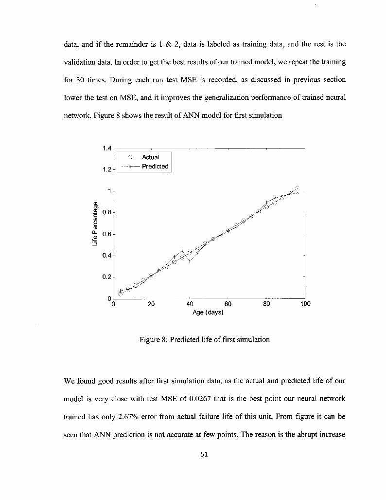
data, and if the remainder is 1 & 2, data is labeled as training data, and the rest is the

validation data. In order to get the best results of our trained model, we repeat the training

for 30 times. During each run test MSE is recorded, as discussed in previous section

lower the test on MSE, and it improves the generalization performance of trained neural

network. Figure 8 shows the result of ANN model for first simulation

1.4

1.2

1

?

I 0.8?

?

% °·6

0.4

0.2

-?— Actual?«— Predicted

40 60

Age (days)

Figure 8: Predicted life of first simulation

We found good results after first simulation data, as the actual and predicted life of our

model is very close with test MSE of 0.0267 that is the best point our neural network

trained has only 2.67% error from actual failure life of this unit. From figure it can be

seen that ANN prediction is not accurate at few points. The reason is the abrupt increase

51

and decrease of the stress level the age point 40 and 80 till it fails. This there is a sudden

shift at point 40, where stress level during simulation is increased, and ANN during

generalization process consider this shift as a sudden change in input parameters and give

short time errors, but soon after it takes successive normalized values it reduces the error,

again on age point 80, where there is decreased in stress level ANN has shown error,

because of same problem.

4.3.2.3. ANN Model Prediction Results for the Second Simulation Data

In the second simulation of the generation of accelerated life failure data under time

varying condition, we set the threshold value at 700. That is a unit is considered failed

when stress level crosses 700 for this simulation. The diffusion parameter sigma ( s? ) is

set at 0.9. Again the stress level is increasing in this simulation the same way as we did in

the first simulation and the unit fails at 99 days. Figure 9 shows the second set of

simulated data. As can be seen, with larger sigma value, the fluctuation of the sigma

becomes larger, and more noise is introduced in the signal.

52

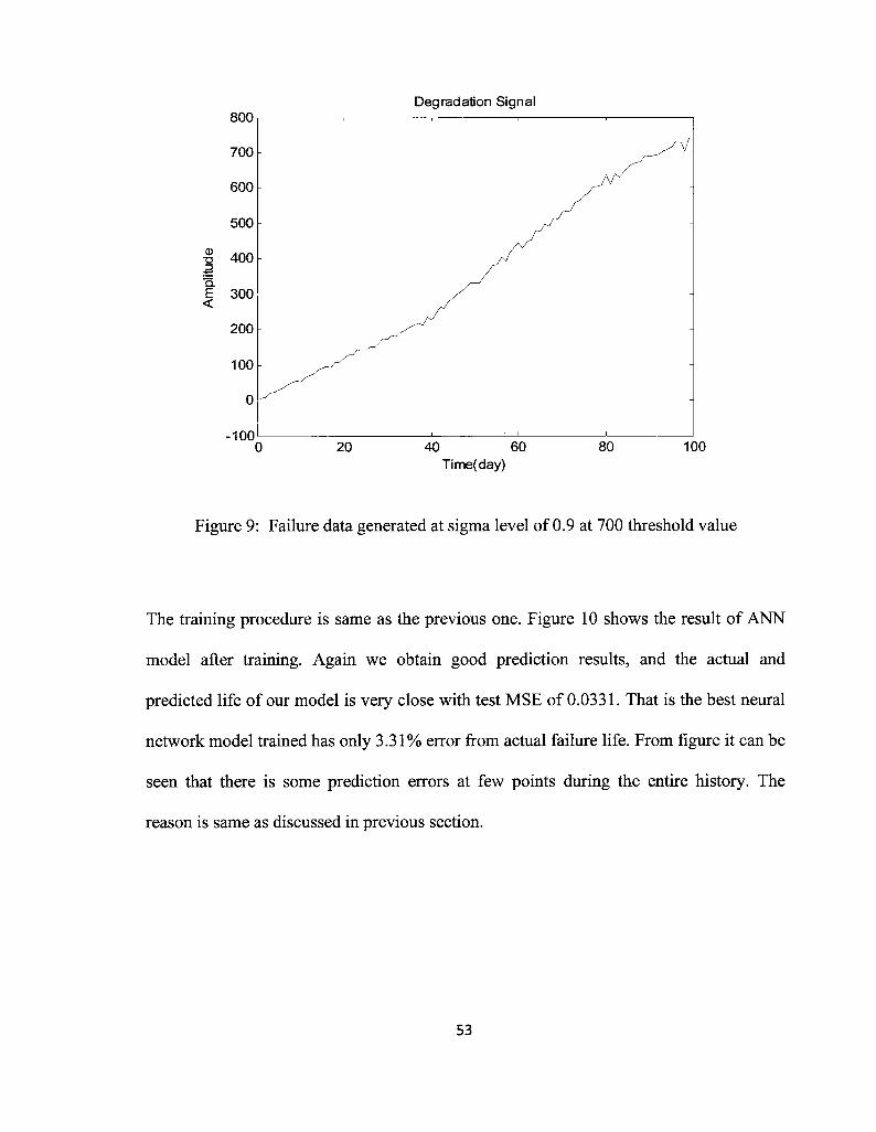
Degradation Signal

E 300

20 40 60Time(day)

100

Figure 9: Failure data generated at sigma level of 0.9 at 700 threshold value

The training procedure is same as the previous one. Figure 10 shows the result of ANN

model after training. Again we obtain good prediction results, and the actual and

predicted life of our model is very close with test MSE of 0.0331. That is the best neural

network model trained has only 3.31% error from actual failure life. From figure it can be

seen that there is some prediction errors at few points during the entire history. The

reason is same as discussed in previous section.

53

Actual* Predicted

S 0.8

20 40 60Age (days)

100

Figure 10: Predicted life of Second simulation

4.4. Summary

In this chapter, we discussed our RUL prediction scheme, and the proposed feedforward

neural network model. We proposed a model with two versions. The first version with

five inputs can handle the discrete data points, where the interval of inspection is not

constant. In the second version, we modify the model. For this research purpose as the

interval of sampling is constant, we do not need to feed previous data time as an input.

Therefore instead of five we feed only four inputs in this model. We discuss the training

of neural network model and its validation with simulated data. This proposed model is

not only applicable to bearings but also it can be applied to other rotary components, like54

gears. The only thing need to be done is the selection of condition health monitoring

parameters, also input of health condition monitoring parameters can also be increased

with less modification and the same model can be used for RUL prediction.

55

Chapter 5

Experiments Setup and Validation ofANN Model

This chapter contains detailed information of our experiment setup for bearing

prognostics, and validation of our neural network model with the data generated through

run to failure tests. We used bearing prognostic simulator for failure tests. Some detailed

are provided for this equipment along with data acquisition system of our research work,

and results of accelerated life failure tests. In the last section we have demonstrate the

results, we validate the proposed ANN prediction approach using the real signals collects

from the experiments.

5.1. Bearing Prognostics Simulator

Bearing prognosis requires bearing failure data at certain interval for the calculation of

remaining useful life. In practices if we take data from industry, it will be a time

consuming process. We decided to conduct our research using Bearing Prognostics

Simulator of Spectra Quest Company, so that we can perform accelerated life testing of

bearings for our research purposes. Figure 1 1 gives the basic picture of our simulator

56

saa·a··«

*ct

aj, ?

te'»"5*

Figure 1 1 : Bearing Prognostics simulator

Spectra Quest's Bearing Prognostics simulator (BPS) is specially designed to conduct

fundamental research in bearing wear, and modeling bearing damages and failures

evolution process. It provides an opportunity to develop a predictive model of bearing

remaining life based condition monitoring measurement. Working phenomena of this

equipment is application of load in radial direction, and this load can be measured by

frictional torque measuring system. This equipment can be driven in either a constant

speed, or purely oscillatory motion and oscillatory excitation superimposed on rotation

through stepper motor.

57

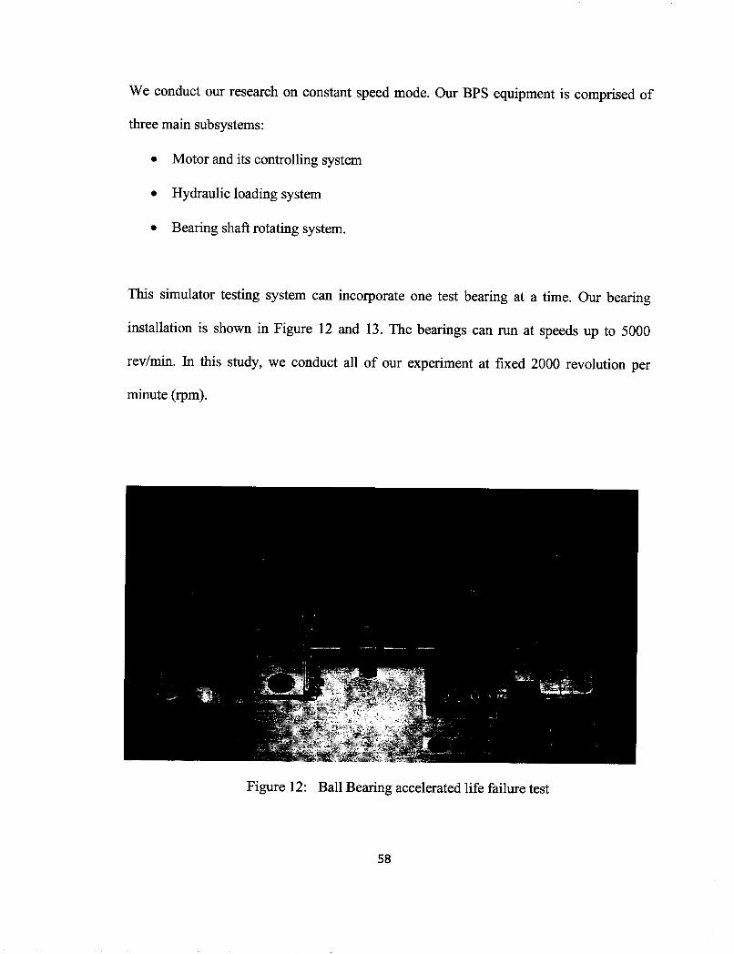
We conduct our research on constant speed mode. Our BPS equipment is comprised ofthree main subsystems:

• Motor and its controlling system

• Hydraulic loading system

• Bearing shaft rotating system.

This simulator testing system can incorporate one test bearing at a time. Our bearinginstallation is shown in Figure 12 and 13. The bearings can run at speeds up to 5000rev/min. In this study, we conduct all of our experiment at fixed 2000 revolution perminute (rpm).

Figure 12: Ball Bearing accelerated life failure test

58

FRI Test BaB Bearne

BW" .

2SW3?.

*.'-

Jf.· '. ,· -

5.1.1. Load

Figure 1 3 : Failed ball bearing after test

We conduct two test at 2500 and 3000 lbs at fixed rpm to investigate the bearing failuretime under varying load conditions. In these tests both load and rpm were fixed from start

to end of the test till bearing get failed. Data is collected for estimation of bearing RULunder time variant conditions.

59

5.1.2. Test Bearings

The test bearings used in our experiments are single groove SKF ball bearings, 62052

RSC3, as shown in Figure 14

Figure 14: KOYO 62052 Ball Bearing used in the research

With the application of load, which is beyond the normal operating condition of bearings,

after only few hours of operation, damage starts with small cracks. These cracks are

located between the surface of the flat track and the rolling elements, usually referred to

as spall propagation, as previously discussed in literature review. The spalls gradually

propagate till the failure of bearing signed is observed and experiment is finished.

60

5.2. Data Acquisition and Signal Processing

Data acquisition is the process of acquiring information of equipment existing health

condition, through method of continuous sampling at selected intervals. Normally data is

collected in an analog form through sensors. Then with the help of special software, it is

converted into digital format for further processing and feature extraction. Signal

detection algorithm for bearing condition monitoring is important part for predictive

maintenance of equipments. Selection of desired features and their relevant features plays

a vital role for both diagnostic and prognostics purposes. Accurate prediction of bearing

impended faults can lead to proper time of adjustment and replacement in order to avoid

catastrophic failures of the whole equipment.

The basic purpose of data acquisition of vibration or any other signals is to measure the

changes in equipments conditions. Whenever structural distress occurs, it appears in form

of relative motion of entire components in the form of vibration. Thus with the help of

sensors, this variation is measured and processed in order to build either the fault

diagnosis models or prognosis models. This research work is dedicated to prognosis of

rolling element bearing under time variant conditions. Figure 15 shows the basic layout

of the work followed in this research. Normally bearings are selected, based on life

calculation as per their industrial application and operating factors, and their actual life is

affected by operation and environmental effects.

61

Vibration Sensor

Actuator ¦¦wmsnMEam

¦SBïetlÎ^SSeï

Vibration Data

Figure 15: Proposed approach for bearing prognostics

62

5.2.1. Vibration measuring Sensor

We use piezoelectric sensor, which is case mounted to our test bearing support housing.

It was an IMI 608 Al 1 model sensor as shown in Figure 11.

Figure 16: Vibration Sensor

5.2.2. Data Acquisition unit

We used National Instrument "High speed USB carrier NSI USB-9162" unit for

collection of data through vibration sensor. The sampling frequency of this unit 25 KHz,

therefore it can sample 25000 data points of vibration amplitude for one second, shown in

Figure 17.

63

HEwmgB&üsi;

wfflfflÈsmmm®

IS 'TÉ¿tWdrfSrun

I51 11%

H

SS C¿.(?a

M ?

¦

tsœiN

Figure 1 7: Data Acquisition unit

5.2.3. Signal Processing Software

We use National Instruments Lab View Signal Express 2009, software for the collection

of vibration data. We utilize its function for capturing time domain data and pre selected

sampling time and interval. The rest of the processing and analysis are performed through

Matlab programs for signal processing and neural network training.

64

S* I* &- I^ «Ig« ®??* lötfr- ö#Quasi» ¦ Um · •',t-niv+.i.mxi *

with m kcc&tmmttm*im%f *#&##*

IfBPS-,M'5I,W»Í MiSKÍSS»» i*vœ-vs>m

fcí.r.-» ?-???»*ft » T^Wr

ÉSnieiï Wife

:-=??;.:·.-: :.-' ¡.-'fe m-tt

* .-.tWaamiifntmnt

»Ol»«»!»»«·!

Figure 18: Vibration amplitude data collection for Prognostics test

5.2.4. Sampling

During accelerated life tests of bearings we collected samples after every four minutes

for the duration of two seconds, in order to get overall amplitude of bearing vibration

signatures at inspection points.

65

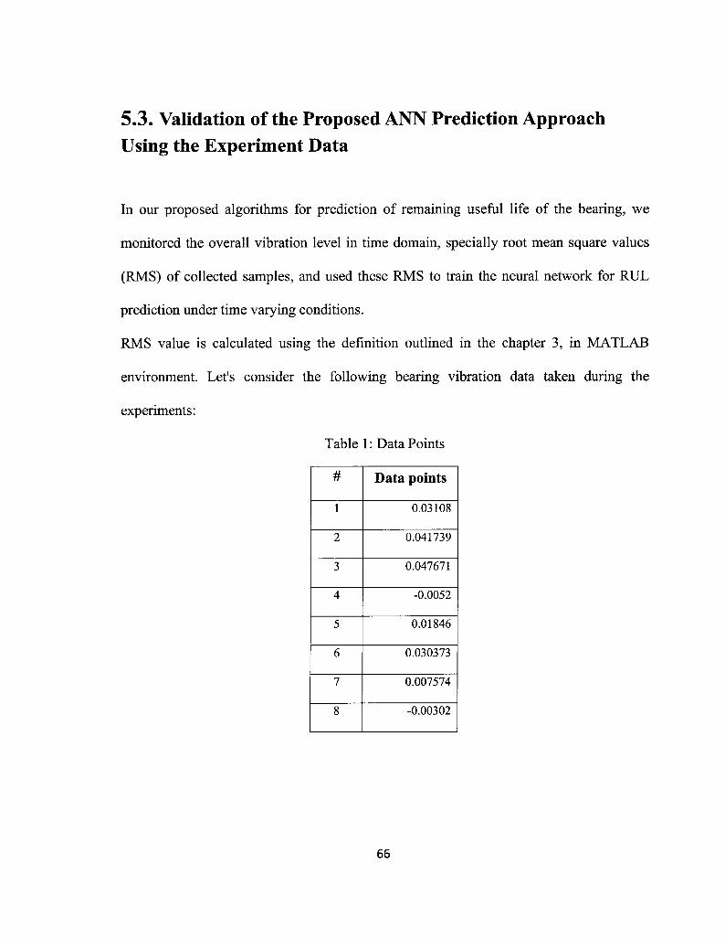
5.3. Validation of the Proposed ANN Prediction ApproachUsing the Experiment Data

In our proposed algorithms for prediction of remaining useful life of the bearing, we

monitored the overall vibration level in time domain, specially root mean square values

(RMS) of collected samples, and used these RMS to train the neural network for RUL

prediction under time varying conditions.

RMS value is calculated using the definition outlined in the chapter 3, in MATLAB

environment. Let's consider the following bearing vibration data taken during the

experiments:

Table 1 : Data Points

# Data points

0.03108

0.041739

0.047671

-0.0052

0.01846

0.030373

0.007574

-0.00302

66

Using the definition:

Signal (RMS) = !±¿(5,)'

Table 2: RMS Calculation

0.03108 0.03108 0.03108 0.03108 0.03108 0.03108 0.03108 0.03108

($f 0.000966 0.000966 0.000966 0.000966 0.000966 0.000966 0.000966 0.000966

S ??/)2 =0.006578i=l

N=8

Signal (RMS) = J- * 0.006578 =0.02867

5.3.1. The First Experiment

First experiment is conducted at the load of 2500 lbs, at 2000 rpm. Data is collected

through vibration sensor and processed in lab view. Theoretically RMS value of bearing

is generally constant when it has no defect and it starts increasing gradually when fault

67

occurs. We practically observed these phenomena during the test. When it is close to fail,

there is sharp increase in overall amplitude of bearing vibration causing RMS value to

increase, till a point where weird noises start and severe vibration show in the equipment.

We set a threshold value of 0.12 RMS for bearing to be considered failed during the

training of our neural network. The total duration of bearing failure under this condition

is 952 minutes. Figure 19 shows the overall RMS value of entire test.

RMS

?

CU

RMS Threshold

0.040 100 200 300 400 500 600 700 800 900 1000

Time(Mitnute)

Figure 19: RMS values of first experiment at 2500 lbs of load

68

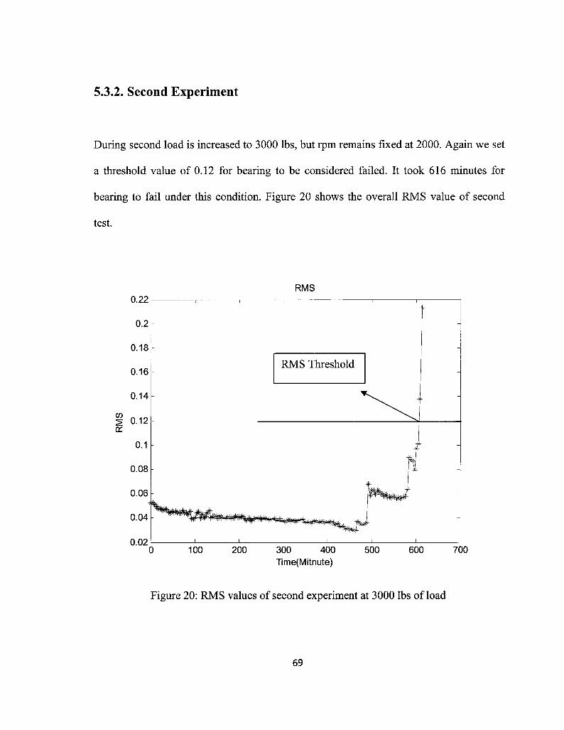
5.3.2. Second Experiment

During second load is increased to 3000 lbs, but rpm remains fixed at 2000. Again we set

a threshold value of 0.12 for bearing to be considered failed. It took 616 minutes for

bearing to fail under this condition. Figure 20 shows the overall RMS value of second

test.

RMS0.22

0.2

0.18

0.16

0.14

i 0.120.1

0.08

0.06

0.04

0.020 100 200 300 400 500 600 700

Time(Mitnute)

Figure 20: RMS values of second experiment at 3000 lbs of load

69

RMS Threshold

5.4. Prediction results with Proposed Neural Network Model

The training method use for experiment data is same as we did with simulation data. That

is to improve neural network generalization capability, we use network validation method

by dividing the available data into the training set and the validation set. Data in the

training set is used to adjust the ANN weights and bias values, while the data in the

validation set is not. For training purpose, we combine the two failure histories of

accelerated life test, and set a threshold RMS value of 0.12. This means in both of the

failure histories under varying time condition, bearing are considered failed if their RMS

values reached 0.12. Therefore in the histories RMS values of the vibration signature are

determined and fed to our neural network model in Matlab. We input 238 inspection

points in the first failure history at 2500 lbs, and 154 inspection points in the second

history at 3000 lbs of load to our neural network model. Failure time for the first history

was 952 minutes and for the second history it was 616 minutes. We check their age

values at the corresponding RMS value of 0.12, and fed these values in our training

model to set a threshold for individual histories with respect to RMS value of 0.12. Again

we divide the available data into the training set, the validation set, and the test set. We

use 25% of the available data as the validation set, 25% as the test set, and the other 50%

as the training data set. In order to check the performance of neural network model, we

select the MSE on the test data set. During training for better generalization performance,

we ran it for 30 times in order to get the best ANN model corresponding to the lower

70

validation. Result of our model with the time varying data of actual bearing accelerated

life failure is shown in figure 21 .

ActualPredicted

B 0.8

0 100 200 300 400 500 600 700 800 900 1000Age (days)

Figure 2 1 : Predicted life of time varying data with neural network model

The result shows a significant progress towards the goal of creating a model of a

prognostic system for bearings. Two sets of failure histories were feed to train the ANN.

Both the failure histories are under different loading conditions, the result demonstrates,

that proposed ANN model, with the input of RMS as a condition monitoring data, time

and load factor has the capability to forecast bearing remaining useful life under time

71

varying condition. As the training criteria were set at lowest test MSE, our proposed

model has predicted the RUL with test MSE of 0.04. This shows the error of only 4%

from actual versus predicted life from our model. Two time points input for training

purpose of ANN has give better generalization performance. Another aspect of this

model is its training algorithm, we use resilient back propagation algorithm for RUL

prediction, and it has shown good results. Our result reflects that this model has good

capability to handle the data for this specific research for RUL prediction under time

varying conditions. Our proposed methodology can handle both linear and non linear

degradation data, to determine the current state bearings in terms of accumulated life, and

a future state of forecasting technique, to predict the time to failure when components are

subjected to different loading conditions during their operation. The results also

demonstrate the effectiveness of the proposed method in dealing with real-world

condition monitoring data for health condition prediction. The application of this model

is not limited to bearings, but it can be applied to any other rotary equipment, once the

health condition indicators are selected.

72

Chapter 6

Conclusions and Future Work

6.1. Conclusions

This research work is done on prognostics of bearings under time varying condition.

Bearings are key mechanical components of rotary machines. Failure of these

components can stop the operation and result in financial losses, which are much higher

than the cost of bearing. Remaining useful life prediction of bearings under time varying

condition is a challenging task as a research work. The existing RUL prediction work

available is limited to fixed operating conditions (e.g., pressure, temperature, humidity,

rotating speed, and load). However, in many applications, such as some wind turbine,

transmission and engine applications, the load that the equipment is subject to changes

over time. It is critical to incorporate the changing load in order to produce more accurate

prognostics methods.

A data-driven life prediction model for rolling element bearings failure under time

varying condition has been developed using neural network. The proposed method can be



measurement values as inputs, a new input neuron is introduced to incorporate the

varying loading condition. The output of the ANN model is life percentage, based on

73

which the remaining useful life can be calculated once the ANN is trained. Two sets of

simulated degradation data under time varying load are used to demonstrate the











method in dealing with real-world condition monitoring data for health condition



6.2. Future Work

Based on the research work in this thesis, we can further explore the following research

topics:

• Conduct more experiments on different types ofbearings for RUL prediction.

• Study remaining useful life prediction of bearings under other time varying

operating condition like speed and temperature.

74

• Investigate the acoustic emission technology for RUL prediction of rolling

element bearings and other equipments.

• Develop other data driven and physic based models for prognostics of rolling

element bearings.

Bibliography

1. Abd, M., Sharifah, S., & Takashi, H. (2010). Predicting Remaining useful Life of

Rotating Machinery based on Artificial Neural Network. Computers and

Mathematics with Applications, Vol.60, 1078-1087

2. Bin, Z., Georgios, G., Marcos, O., Abhinav, S., Douglas, B., George, V., &

Steven, L. (2008). Rolling Element Bearing Feature Extraction and Anomaly

Detection Based on Vibration Monitoring. 16th Mediterranean Conference on

Control and Automation Congress Centre, France.

3. Carey. M., & Koenig. R. (1991).Reliability Assessment Based on Accelerated

Degradation: A Case Study. IEEE Transactions on Reliability, Vol. 40, 499-506.

4. Chaudhary. A. & Tandon.N. (1998). A Theoretical Model to Predict Vibration

Response of Rolling Bearings to Distributed Defects under Radial Load. Journal

of Vibration and Acoustics, Transactions, ASME, Vol. 120, 214-220.

5. David He, Eric, B. (2007). Development and Validation of Bearing Diagnostic

and Prognostic Tools using HUMS Condition Indicators. Aerospace Conference,

pp: 1-8

6. Dyer. D., & Stewart, R. M. (1978). Detection of Rolling Element Bearing

Damage by Statistical Analysis. ASMEJ. Mech. Des, Vol. 100, 229-235.

76

7. Eric Y. Kim., Andy C. C. Tan., Bo-Suk, Y., & Vladis, K. (2007). Experimental

Study on Condition Monitoring of Low Speed Bearings: Time Domain Analysis.

5th Australasian Congress on Applied Mechanics, ACAM, Brisbane, Australia

8. Fulong, Lu., & Hongbing. Ji., & Zhao. X. (1993). The ML Bearing Estimation by

using Neural Network Journal ofElectronics, VoIA, 1-8

9. Gebraeel, N., Lawley, M. A., & Liu, R. (2004). Residual Life Predictions from

Vibration-Based Degradation Signals: A neural network approach. IEEE

Transactions on Industrial Electronics, Vol.5\, 694-700

10. Gebraeel, N., Mark A. Lawley, R., & Jennifer K. Ryan. (2005). Residual-Life

Distributions from Component Degradation Signals: A Bayesian approach. HE

Transactions, Vol. 37, 543-557

11. Gebraeel. N., & Pan J.(2008). Prognostic Degradation Models for Computing and

Updating Residual Life Distributions in a Time-varying Environment. IEEE

Transactions on Reliability, Vol. 57, 539-550.

12. Haitao, 1, & Z, Tian. A General Frame work for remaining useful Life Prediction

for a Single Unit under Time-Varying Operating Conditions.

13. Hongmou, L., & Saleh, Z. (2001). Analysis of Vibration Signal's Time Frequency

Patterns for Prediction of Bearing's remaining useful Life. System Theory,

Proceedings ofthe 33rd South-eastern Symposium, pp 25-29

77

14. Ho. D. & Randall. R. B. (2000). Optimization of Bearings Diagnostic Techniques

using Simulated and Actual Bearing Fault Signals. Mechanical Systems and

Signal Processing, Vol. 14, 763-788

15. Israel, E., & Anna, L., & Robert E. U. (1993). Monitoring and Diagnosis of

Rolling Element Bearings Using Artificial Neural Networks. IEEE Transaction

on Industrial electronics, Vol. 40, 209- 21 7

16. Jack, L.B, & A, K, Nandi. (2000).Genetic Algorithm for Feature Selection in

Machine Condition Monitoring with Vibration Signals. IEEE Proceedings:

Vision, Image and Signal Processing, Vol. 147, 205-212

17. Janjarasjitt. S, Ocak. H., & Loparo, K, A. (2008). Bearing Condition Diagnosis

and Prognosis using Applied Nonlinear Dynamical Analysis of Machine

Vibration Signal. Journal ofSound and vibration, Vol: 317, 112-126

18. Jardine, ?., Lin, D., & Banjevic, D. (2006). A Review on Machinery Diagnostics

and Prognostics Implementing Condition-Based Maintenance. Mechanical System

and Signal Processing, Vol.20, 1483-1510

19. Khemili, L, & M. Chouchane. (2005). Detection of Rolling Element Bearing

Defects by Adaptive Filtering. European Journal ofMechanics A/Solids, Vol. 24,

293-303.

20. Lee, S, K., & P. R. White. (1998). The Enhancement of Impulsive Noise and

Vibration Signals for Fault Detection in Rotating and Reciprocating Machinery.

Journal ofSound and Vibration, Vol. 217,485-50578

21.Li, Bo., Mo-Yuen, C, & James C, H. (2000). Neural-Network- Based Motor

Rolling Bearing Faulty Diagnosis. IEEE Transactions on Industrial Electronics,

Vol Al, 1060-1069

22. Li. Y, Billington, S., C. Zhang, T, Kurfess. S, Danyluk & S, Liang. (1999).

Adaptive Prognostics for Rolling Element Bearing Condition. Mechanical

Systems and Signal Processing, Vol. 13, 103-113.

23. Lybeck. N., Marble, S, & Morton, B. (2007). Validating Prognostic Algorithms:

A Case Study using Comprehensive Bearing Fault Data. IEEE Aerospace

Conference, pp: 1-9

24. Mathworks. The MATLAB Neural Networks toolbox, 2007

25. Marble, S., &. Morton, B.P. (2006). Predicting the Remaining Life of Propulsion

System Bearings. Aerospace Conference, IEEE

26. Martin, KF, & Thorpe, P. (1992) .Normalized Spectra in Monitoring of Rolling

Bearing Elements. Wear, Vol. 159, 153-60.

27. McFadden, P. D., & Smith, J. D. (1984). The Condition Monitoring of Rolling

Element Bearings by the High-Frequency Resonance Technique—A Review.

Tribol Int., Vol. 17, 3-10.

28. Mechefske C, K. (1998). Objective Machinery Fault Diagnosis using Fuzzy

'Logic. Mechanical Systems and Signal Processing, Vol. 12,855-862

79

29. Meeker, W. Q., Escobar, L. ?., & Lu, C. J. (1998).Accelerated Degradation Tests:

Modeling and Analysis. Technometrics, Vol. 40, 89-99.

30. Meyer, LD., Ahlgren, FF., & Weichbrodt, B. (1980). An Analytic Model for Ball

Bearing Vibrations to Predict Vibration Response to Distributed Defects. Trans

ASME, JMech Design, Vol. 102,205-210.

31. Paya, B.A., Esat, LL, & Badi, M.N.M. (1997). ANN Based Fault Diagnostics of

Rotating Machinery using Wavelet Transform as a Pre-processor. Mechanical

Systems and Signal Processing, Vol. 11,751-765

32. Patii, M. S., Jose Mathew, & P, K. R. (2008). Bearing Signature Analysis as a

Medium for Fault Detection: A Review. J. Tribology, Vol. 130, 1-7.

33. Price, E.D, A. W. Lees, & Friswell, M. I. (2001). Application of High Frequency

Monitoring for classification of Rolling Element Bearing Failures. Key

Engineering Materials Vols. 204-205, 173-182

34. R, Huang., Lifeng, Xi., Xinglin, Li., C, R. L., Hai, Q., & Jay, Lee. (2007).

Residual Life Predictions for Ball Bearings Based on Self-Organizing Map and

Back Propagation Neural Network Methods. Mechanical Systems and Signal

Processing, Vol. 21, 193-207

35. Samanta, B. (2004). Gear Fault Detection using Artificial Neural Networks and

Support Vector Machines with Genetic Algorithms. Mechanical Systems and

Signal Processing, Vol. 18, 625-644,

80

36. Samanta, B, Al-Balushi., &.Khamis, R. (2003). Artificial Neural Network Based

Fault Diagnostics of Rolling Element Bearings using Time Domain Features.

Mechanical Systems and Signal Processing, Vol. 17,317—328

37. Samanta. B, Khamis, R., & Saeed A. (2004). Bearing Fault Detection Using

Artificial Neural Networks and Genetic Algorithm. EURASIP Journal on Applied

Signal Processing, Vol. 2004, 366-377

38. Satish, B., & Sarma, N.D.R. (2005). A Fuzzy BP Approach for Diagnosis and

Prognosis of Bearing Faults in Induction Motors, IEEE Power Engineering

Society General Meeting, vol. 3, 2291-2294

39. Sawalhi, N., & Randall, R.B. (2005). Spectral Kurtosis Optimization for Rolling

Element Bearings. Signal Processing and Its Applications, Proceedings of the

Eighth International Symposium, Vol. 2 , 839 - 842

40. Sawalhi, N., & Randall, R.B. (2005). Spectral Kurtosis Enhancement using

Autoregressive Models". ACAM Conference, Melbourne.

41. Shao,Y, & Nezu, K. (1996). An Online Monitoring and Diagnostics Method of

Rolling Element Bearing with AI. Transactions of the Society ofInstrument and

Control Engineers, Vol. 32, 1287-1293

42. Shao,Y., & Nezu, K. (2000). Prognosis of Remaining Bearing Life using Neural

Networks. Proc Instn Mechanical Engineers, Vol. 214, 217-230

81

43. Shiroshi, J., Y, Li., S, Liang., Kurfess, T., & Danyluk, S. (1997).Bearing

Condition Diagnostics via Vibration and Acoustic Emission Measurements.

Mechanical Systems and Signal Processing, Vol. 1,693-705

44. Sreejith, B., Verma, A.K., & Srividya, A. (2008). Fault Diagnosis of Rolling

Element Bearing using Time-Domain Features and Neural Networks. IEEE

Region 10 Colloquium and the Third ICIIS, Kharagpur, INDIA

45. Sorin, Z. (2001). Digital Signal Processing System for Image Pattern Recognition.

Telecommunications in Modern Satellite, Cable and Broadcasting Service, 5th

International Conference, Yugoslavia. Vol.2, 423-425

46. Subrahmanyam. M., & Sujatha, C. (1997). Using Neural Networks for the

Diagnosis of Localized Defects in Ball Bearings. Tribology International, Vol. 30,

739-752

47. Sunnersjo, CS. (1985). Rolling Bearing Vibrations — Geometrical

Imperfections and Wear. Journal ofSound & Vibration, Vol.98, 455-74.

48. Tandon, N. (1994). A Comparison of some Vibration Parameters for the

Condition Monitoring of Rolling Element Bearings. Measurement, Vol.,12, 285-

289.

49. Tandon.N & Choudhary.A. (1997). An Analytical Model for the Prediction of the

Vibration Response of Rolling Element Bearing due to a Localized Defect.

Journal ofsound and vibration, Vol.205, 275-292

82

50. Tandon, N., & Nakra, B. C. (1993). Detection of Defects in Rolling Element

Bearings by Vibration Monitoring. J. Inst. Eng (India), Mechanical Engineering

Division, VoLTi, 271-282.

51. Tian, Z. (2009). An Artificial Neural Network Method for Remaining useful Life

Prediction of Equipment Subject to Condition Monitoring. Journal ofIntelligent

Manufacturing, , pp: 1 -6.

52. Tian, Z., & MJ, Zuo. (2009). Health Condition Prognostics of Gears using a

Recurrent Neural Network Approach. Proceedings of the Reliability and

Maintainability Symposium, Fort Worth, TX, USA

53. Tian, Z., Lin, D., & Wu, B. (2009). Condition Based Maintenance Optimization

Considering Multiple Objectives. International Conference on Industrial

Engineering and System Management. Montreal

54. Tian. Z, Lorna, W, & Nima, S. (2010). A Neural network Approach for

Remaining useful Life Prediction utilizing both Failure and Suspension Histories.

Mechanical Systems and Signal Processing, Vol.24, 1542-1555

55. Vachtsevanos, G, & Wang, P. (2001). Fault Prognosis using Dynamic Wavelet

Neural Networks. Proceedings of IEEE Systems Readiness, Technology

Conference, pp. 857-870.

56. Volker. E, & Martin, HR. (1984). Early Detection of Damage in Rolling Bearings.

ISA Trans, Vol. 23, 27-32.

83

57. Wardle, FP., & Poon, SY. (1983). Rolling Bearing Noise — Cause and Cure.

Chartered Mech Engr pp: 36-40.

58. Washo, MW. (1996). A Quick Method of Determining Root Causes and

Corrective Actions of Failed Ball Bearings. Lubric Eng, Vol. 52, 206-13.

59. Williams, T., Ribadeneira, X., Billington, S., & Kurfess, T. (2001). Rolling

Element Bearing Diagnostics in Run to Failure Life Time Testing. Mechanical

Systems and Signal Processing, Vol. 15,979-993.

60. Wu, S. J., Gebraeel, N., Lawley, M. A., & Yih, Y. (2007). A Neural Network

Integrated Decision Support System for Condition-Based Optimal Predictive

Maintenance Policy. IEEE Transactions on Systems Man and Cybernetics, Vol.

37, 226-236.

61. Yu, JJ, Bently, D.E., Goldman, P., Dayton, K.P., & Van, S.B.G. (2002). Rolling

Element Bearing Defect Detection and Diagnostics Using Displacement

Transducers. Journal ofEngineeringfor Gas Turbines and Power, Vol. 124, 517-

527

62. Zaharí, T & Khusnun, W. (2009). Artificial Neural Network for Bearing Defect

Detection Based on Acoustic Emission. The International Journal of Advanced

Manufacturing Technology, pp 1-8

63. Zhang. X, M. T. Le, Seth, B. B. & Liang, S.Y. (2002). Bearing Life Prognosis

under Environmental Effects Based on Accelerated Life Testing. Journal of

Mechanical Engineering Science, Vol.2 1 6, 509-5 1 684

64. Zeng. L., & Wang, Z. (1991). Machine Fault Classification: A Fuzzy Approach.

The International Journal of Advanced Manufacturing Technology,

Vol. 6, 83-94

65. Zhen, Li., Zhengjia, He, Yanyang, Z., & Chen, X. (2008).Bearing Condition

Monitoring Based on Shock Pulse Method and Improved Redundant Lifting

Scheme Source. Mathematics and Computers in Simulation archive, Vol. 79, 318-

338

85

BEARING PROGNOSTICS USING NEURAL NETWORK ...ABSTRACT Bearing Prognostics using Neural Network under...

Documents

Transcript of BEARING PROGNOSTICS USING NEURAL NETWORK ...ABSTRACT Bearing Prognostics using Neural Network under...