Prof. Dr. Josef Brüderl LMU München April 2015 · – Josef Brüderl, Panel Analysis, April 2015...
293
Applied Panel Data Analysis Using Stata Prof. Dr. Josef Brüderl LMU München April 2015
Transcript of Prof. Dr. Josef Brüderl LMU München April 2015 · – Josef Brüderl, Panel Analysis, April 2015...

Applied Panel Data AnalysisUsing Stata
Prof. Dr. Josef BrüderlLMU München
April 2015

Contents II) Panel Data 06
II) The Basic Idea of Panel Data Analysis 17
III) An Intuitive Introduction to Linear Panel Regression– A Didactic Example 21– Within Estimation (Fixed-Effects Regression) 30– Within Estimation With Control Group 47
IV) The Basics of Linear Panel Regression– Linear Panel Models 51– Fixed- or Random-Effects? 63
V) A Real Data Example: Marriage and Happiness – Preparing Panel Data 70– Describing Panel Data 78– The Results 81– Interpreting Results from Panel Regressions 95
Josef Brüderl, Panel Analysis, April 2015 2

Contents IIVI) Modeling Individual Growth
– Growth Curve Models 117– The Age-Period-Cohort Problem 129– Group Specific Growth Curves 139
VII) Further Linear Panel Models– Alternative Within Estimators 147– The Fixed-Effects Individual-Slopes Model 155– Mixed-Coefficients Panel Models 174– The Hybrid Model 188– Dynamic Panel Models 197– Comparing Models by Simulations 205– Panel Regression with Missing Data 210
Josef Brüderl, Panel Analysis, April 2015 3

Contents IIIVIII) Non-Linear Panel Models: Fixed-Effects Logit 218
IX) Event History Analysis with Repeated Events 225– Example: Duration of Unemployment
X) Limitations of the Within Methodology– Limitations of Scope 237– Violations of Strict Exogeneity 243– Consequences of Panel Attrition 256– Consequences of Panel Conditioning 260– Direction of Causality 262
XI) Final Remarks on Panel Analysis– Panel Regression and Causal Inference 267– The FE Revolution in Social Research 274– Some Critical Remarks on the Literature 284
References 289
Josef Brüderl, Panel Analysis, April 2015 4

What This Lecture Aims For• Introducing basic methods of panel data analysis (PDA)
– Emphasis on fixed-effects and growth curve methods– Complex methods are de-emphasized
• Practical implementation of PDA with Stata– Important Stata commands are on the slides– The lecture is accompanied by Stata do-files (and data), whereby all
computations can be reproduced
• Presenting and interpreting results– The graphical display of regression results is emphasized
- The era of the regression table is over!
• Teaching materials can be found here – Stata Do-Files, Stata Commands for Longitudinal Analysis– www.ls3.soziologie.uni-muenchen.de/teach-materials/index.html
Josef Brüderl, Panel Analysis, April 2015 5

Chapter I: Panel Data
Josef BrüderlApplied Panel Data Analysis

Josef Brüderl, Panel Analysis, April 2015
Hierarchy of Data Structures
Time
State
employed
unemployed
• Cross-sectional data – “Snapshot” at one time point
• Panel data – Repeated measurement
• Event history data – Information on the complete life course
The life courses of three individuals
7
Josef Brüderl, Panel Analysis, April 2015
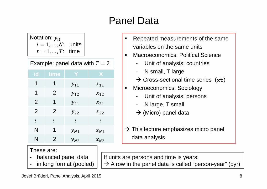
Panel Data Repeated measurements of the same
variables on the same units Macroeconomics, Political Science
- Unit of analysis: countries- N small, T large Cross-sectional time series (xt)
Microeconomics, Sociology- Unit of analysis: persons- N large, T small (Micro) panel data
This lecture emphasizes micro panel data analysis
8
id time Y X1 11 22 12 2⋮ ⋮ ⋮ ⋮N 1N 2
Notation: 1, … , : units1,… , : time
Example: panel data with 2
These are:- balanced panel data- in long format (pooled)
If units are persons and time is years: A row in the panel data is called “person-year” (pyr)

Josef Brüderl, Panel Analysis, April 2015
The Two Major Advantages of Panel Data
• Panel data allow to identify causal effects under weaker assumptions (compared to cross-sectional data)– With panel data we know the time-ordering of events– Thus we can investigate how an event changes the outcome
• Panel data allow to study individual trajectories – Individual growth curves (e.g. wage, materialism, intelligence)
- One can distinguish cohort and age effects– Transitions into and out of states (e.g. poverty)
9

Usage of Panel Data is on the RiseNumber of publications using the SOEP
Josef Brüderl, Panel Analysis, April 2015 10
Source: Schupp, J. (2009) 25 Jahre Sozio-oekonomisches Panel. ZfS 38: 350-357.
According to Young/Johnson (2015) 61% of all empirical articles published in JMF 2010-2014 used panel data. Methods used:
19% event history methods 16% linear regression19% fixed effects models 15% logistic regression22% multilevel models (incl. growth curves) 10% structural equation models

Josef Brüderl, Panel Analysis, April 2015
A Few Remarks on Collecting Panel Data• Cross-sectional survey: retrospective questions
– Problems with recall– Often done for collecting event history data
• Prospective panel survey– Panel data
- Ask for the current status/value– Event history data
- Ask what happened since last interview: between wave retrospective questions (electronic life-history calendar)
- Ideally using dependent interviewing (preloads) to avoid the seam effect
• The advantages of panel data are threatened by two methodological problems (s. Chapter X)
- Panel conditioning (panel effect)- Panel mortality (attrition)
• More on panel methodology can be found in Lynn (2009)11
Important Panel Surveys• Household panels
– Panel Study of Income Dynamics (PSID) [since 1968]- The role model for all household panels
– German Socio-Economic Panel (SOEP) [since 1984]– Understanding Society (UKHLS) [since 1991]
• Cohort panels– British Cohort Studies: children born 1958, 1970, 2000– National Longitudinal Survey of Youth (NLSY79): U.S. cohort born around 1960
• Panels on special populations in Germany recently started– German Family Panel (pairfam), National Educational Panel Study (NEPS),
Survey of Health, Ageing and Retirement in Europe (SHARE), Panel "Arbeitsmarkt und soziale Sicherung" (PASS), TwinLife, Children of Immigrants (CILS4EU), Nationale Kohorte
• Online panel surveys– LISS panel: A Dutch online panel survey– German internet panel (GIP)– GESIS Panel
• Links on German studies you can find here: http://www.ratswd.de/forschungsdaten/fdz
Josef Brüderl, Panel Analysis, April 2015 12
SOEPHousehold Panel Study• Sample of households in Germany• Every person aged 17 or older is interviewed• For persons under 17 proxies are interviewed• When a person moves out of the household, he or she is
followed• Persons, households and original households can be
identified beyond waves• First wave 1984 (subsamples A and B)• Annual interviews (PAPI questionnaire)• Several refreshment subsamples
– Meanwhile about 60,000 persons participated in the SOEP
More information: http://www.diw.de/soepJosef Brüderl, Panel Analysis, April 2015 13

The German Family Panel (pairfam)• Target population
– All German residents, who are able to do an interview in German– Cohort-sequence design: 1971-73, 1981-83, 1991-93
• Sample– Random sample from population registers
- 343 “Gemeinden” were sampled- 42.000 addresses were drawn randomly from the population registers
– Response rate in wave 1: 37 %• Interview mode
– 60 minute CAPI (some parts CASI)• Multi-actor design
– Anchor person (AP) and partner, parents, children• First wave in 2008
– Waves annually, currently wave 7 is in the field– Non-monotonic design: respondents can drop out for one wave
• Data: currently version 5.0 is available– www.pairfam.de
Josef Brüderl, Panel Analysis, April 2015 14

Response Rate Anchor – Panel Stability
Josef Brüderl, Panel Analysis, April 2015 15

Number of Anchors
Josef Brüderl, Panel Analysis, April 2015 16

Chapter II: The Basic Idea of Panel Data Analysis
Josef BrüderlApplied Panel Data Analysis
Josef Brüderl, Panel Analysis, April 2015
Paul Lazarsfeld on Panel Data AnalysisPrinceton „radio project“ (1937-1939)– Research question
Effect of radio ownership on political attitudes:Will the Americans become communist?
– Inference from cross-sectional (control group) or panel data?
“Most of the control groups available for social research are ‘self-selected’.”
“If we give radios to a number of farmers and then notice considerable differences without any great external changes occurring at the same time, it is safer to assume that these differences are caused by radio than it would be, if we were to compare radio owners with non-owners.”
Lazarsfeld/Fiske (1938) The “panel” as a new tool for measuring opinion. Public Opinion Quarterly 2: 596-612.
18

Josef Brüderl, Panel Analysis, April 2015
The Basic Approach• According to the counterfactual approach to causality (Rubin‘s
model) an individual causal effect is defined asΔ , , , : treatment, : control
– However, this is not estimable (fundamental problem of causal inference)• Estimation with cross-sectional data
Δ , ,
– We compare different persons and (between estimation)– Assumption: unit homogeneity (no unobserved heterogeneity)
• Estimation with panel data IΔ , ,
– We compare the same person over time and (within estimation)– Assumption: temporal homogeneity (no period effects, no maturation)
• Estimation with panel data IIΔ , , , ,
– Within estimation with control group– Assumption: parallel trends
19

The Basic Approach• Between estimation works well with experimental data
– Due to randomization units will differ only in the treatment
• However, with observational data between estimation generally will not work, because the strong assumption of unit homogeneity will not hold– Due to self-selection into treatment– Unobserved unit heterogeneity will bias between estimation results
• Within estimation with control group, however, will often work, because the parallel trends assumption is much weaker– Unobserved unit heterogeneity will not bias within estimation
results– Only differing time-trends in treatment and control group will bias
within estimation results
Josef Brüderl, Panel Analysis, April 2015 20

Chapter III: An Intuitive Introduction to Linear Panel
Regression
Josef BrüderlApplied Panel Data Analysis
Section: A Didactic Example

Josef Brüderl, Panel Analysis, April 2015
Is There a Marital Wage Premium for Men?
• Fabricated data: long-format. list id time wage marr, separator(6)
------------------------- -------------------------| id time wage marr | | id time wage marr ||-------------------------| |-------------------------|
1. | 1 1 1000 0 | 13. | 3 1 2900 0 |2. | 1 2 1050 0 | 14. | 3 2 3000 0 |3. | 1 3 950 0 | 15. | 3 3 3100 0 |4. | 1 4 1000 0 | 16. | 3 4 3500 1 |5. | 1 5 1100 0 | 17. | 3 5 3450 1 |6. | 1 6 900 0 | 18. | 3 6 3550 1 |
|-------------------------| |-------------------------|7. | 2 1 2000 0 | 19. | 4 1 3950 0 |8. | 2 2 1950 0 | 20. | 4 2 4050 0 |9. | 2 3 2050 0 | 21. | 4 3 4000 0 |10. | 2 4 2000 0 | 22. | 4 4 4500 1 |11. | 2 5 1950 0 | 23. | 4 5 4600 1 |12. | 2 6 2050 0 | 24. | 4 6 4400 1 |
|-------------------------| |-------------------------|
22
Data: Wage Premium.dtaDo-File: Wage Premium.do
Josef Brüderl, Panel Analysis, April 2015
Is There a Marriage-Premium for Men?0
1000
2000
3000
4000
5000
EU
RO
per
mon
th
1 2 3 4 5 6Time
before marriage after marriage
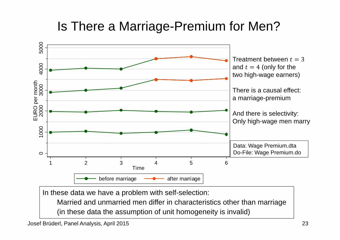
Treatment between 3and 4 (only for thetwo high-wage earners)
There is a causal effect: a marriage-premium
And there is selectivity: Only high-wage men marry
23
Data: Wage Premium.dtaDo-File: Wage Premium.do
In these data we have a problem with self-selection:Married and unmarried men differ in characteristics other than marriage (in these data the assumption of unit homogeneity is invalid)

Josef Brüderl, Panel Analysis, April 2015
How High is the Marriage-Premium?• These are observational (non-experimental) data
– Treatment assignment is not under control of the researcher (no randomization)
- Instead, men can self-select into treatment (marriage)- Therefore, a between approach will be strongly biased (see below)
• A within approach to compute the marriage-premium– We have before ( 1, 2, 3) and after ( 4, 5, 6) measurements– This allows for a within approach.
- This “compensates” for the missing randomization (unit heterogeneity will not bias estimation)
- Thus, we can identify the causal effect despite of self-selection
– Because we also have a control group we can use within estimation with control group (estimation with panel data II)
- Difference-in-differences (DiD)
24

Josef Brüderl, Panel Analysis, April 2015
How High is the Marriage-Premium?• DiD is a after-before comparison with control group
– After-before changes (Δ ) treatment group‐ Δ 4500 4000 500‐ Δ 3500 3000 500
– After-before changes (Δ ) control group‐ Δ 2000 2000 0‐ Δ 1000 1000 0
– To get the average treatment effect (ATE) we take the difference of the averages in treatment and control group
Δ ∈ Δ ∈500 500
20 02 500
– The marriage-premium in our data is +500 €
• In the following we will investigate, whether different statistical regression models can recover this causal effect!
25
Δ13
13
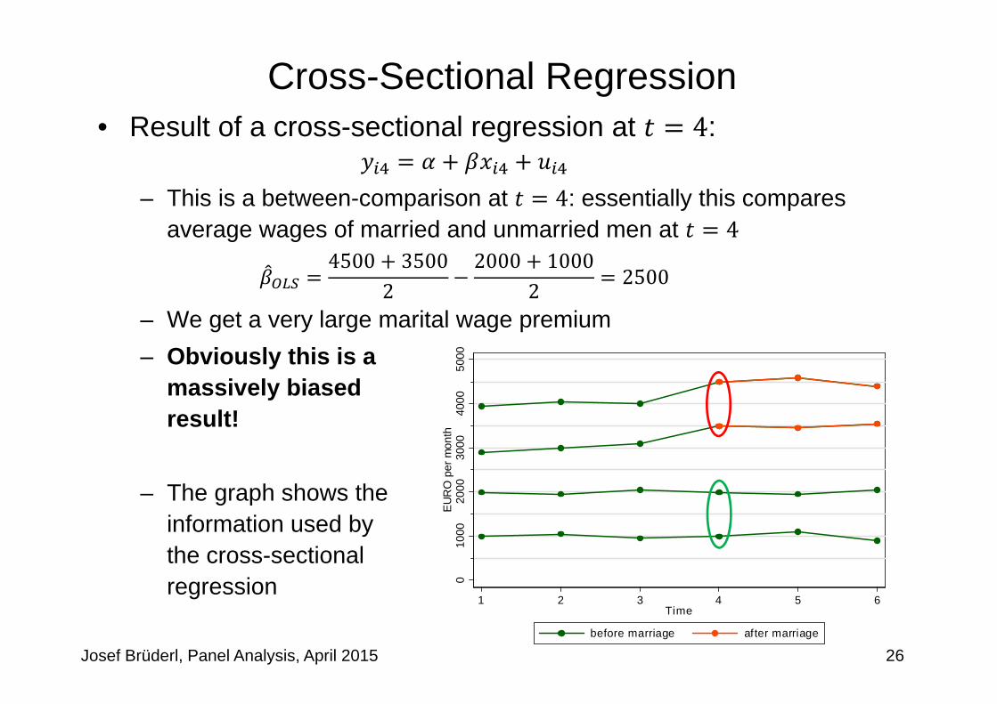
• Result of a cross-sectional regression at 4:
– This is a between-comparison at 4: essentially this compares average wages of married and unmarried men at 4
4500 35002
2000 10002 2500
– We get a very large marital wage premium– Obviously this is a
massively biased result!
– The graph shows theinformation used by the cross-sectionalregression 0
1000
2000
3000
4000
5000
EUR
O p
er m
onth
1 2 3 4 5 6Time
before marriage after marriage
Josef Brüderl, Panel Analysis, April 2015
Cross-Sectional Regression
26

What Is the Problem With Cross-Sectional Regression?• The most critical assumption of a linear regression
is the exogeneity assumption: E | 0– I.e., the error term and the regressor must be statistically independent– The exogeneity assumption implies:
‐ E 0 The (unconditional) mean of the error term is 0‐ Cov , 0 The error term does not correlate with
– The exogeneity assumption guarantees unbiasedness [ ] and consistency [plim ] of the OLS estimator
• Unfortunately, in many non-experimental social science research settings the exogeneity assumption will be violated– The error term and the regressor are dependent
E | 0– Then it is said: the regressor is endogenous (endogeneity)
- The variation that is used to identify the causal effect is endogenous
– will be biased (and inconsistent)
Josef Brüderl, Panel Analysis, April 2015 27

What Is the Problem?• Where does endogeneity come from?
– There are unobserved confounders (unobservables that affect both and )
- Then and the error term are correlated- This is called „unobserved heterogeneity“
or „omitted variable bias“– affects also (reverse causality)
- E.g., high-wage men are selected into marriage,because the higher wage makes them more attractive marriage partners
• The underlying mechanism: self-selection– Treatment and control groups are not built by randomization– Instead, human beings decide according to unobservables or
even the value of , whether they go into treatment or not
• Endogeneity is ubiquitous in non-experimental research Many (most?) cross-sectional regression results are biased! Be critical with cross-sectional results. Always ask, whether
endogeneity might have distorted the results?Josef Brüderl, Panel Analysis, April 2015 28
wagemarriage
intelligenceattractivity
cosmeticsurgery

010
0020
0030
0040
0050
00E
URO
per
mon
th
1 2 3 4 5 6Time
before marriage after marriage
Josef Brüderl, Panel Analysis, April 2015
No Solution: Pooled-OLS• Pool the data and estimate an OLS regression (POLS)
– The result is 1833– This is the mean of the red points - the mean of the green points– The bias is still heavy– The reason is that POLS
also relies on a between comparison
– Panel data per se do not help to identify a causal effect!
– One has to use appropriate methods of analysis to make full advantage of panel data
29

Chapter III: An Intuitive Introduction to Linear Panel
Regression
Josef BrüderlApplied Panel Data Analysis
Section: Within Estimation

Josef Brüderl, Panel Analysis, April 2015
The Error Decomposition• To make full advantage of panel data use within estimation
– Within estimators implement a “after-before comparison”
• Starting point: error decomposition
– : person-specific time-constant error term- Assumption: person-specific random variable
– : time-varying error term (idiosyncratic error term)- Assumptions: zero mean, homoscedasticity, no autocorrelation
31
wagemarriage
cosmeticsurgeryintelligenceattractivity

The Error Components Model• This yields the error components model
– Note that the overall constant has been dropped due to collinearity– Generally, one assumes that the error components are
independent from each other: E | , 0- We will neglect this subtlety in the following
• POLS is consistent only, if the regressor is independent from both error componentsE | 0 random-effects assumption
“no (person-specific) time-constant unobserved heterogeneity”
E | 0 contemporaneous exogeneity assumption“no time-varying unobserved heterogeneity”
Josef Brüderl, Panel Analysis, April 2015 32
wagemarriage
cosmeticsurgeryintelligenceattractivity

Josef Brüderl, Panel Analysis, April 2015
First-Differences Estimator (FD)• The random-effects assumption is strong
– How can we get rid of it?• By a differencing transformation we can wipe out the
Subtracting the second equation from the first gives:
Δ Δ Δwhere “Δ” denotes the change from 1to .
– Person-specific errors have been “differenced out”. Time-constant unobserved heterogeneity has been wiped out!
– Pooled-OLS applied to these transformed data provides the first-differences estimator.
• In the psychological literature this model is also called the „change score“ model
33

Assumptions of FD Estimation• The FD-estimator is consistent if
E | 0for sequential exogeneity assumption- Intuition: otherwise Δ and Δ would be correlated
– However, because is not in the differenced equation, E | 0 is no longer required for consistency
- FD identifies the causal effect under weaker assumptions Time-constant unobserved heterogeneity is allowedOnly time-varying unobserved heterogeneity must not be
Josef Brüderl, Panel Analysis, April 2015 34
wagemarriage
cosmeticsurgeryintelligenceattractivity
Δwage
Δmarriage
Δcosmeticsurgery
differencing transformation

Josef Brüderl, Panel Analysis, April 2015
Example: FD-Regression
. regress D.(wage marr), noconstant
Source | SS df MS Number of obs = 20-------------+------------------------------ F( 1, 19) = 39.97
Model | 405000 1 405000 Prob > F = 0.0000Residual | 192500 19 10131.5789 R-squared = 0.6778
-------------+------------------------------ Adj R-squared = 0.6609Total | 597500 20 29875 Root MSE = 100.66
------------------------------------------------------------------------------D.wage | Coef. Std. Err. t P>|t| [95% Conf. Interval]
-------------+----------------------------------------------------------------marr |D1. | 450 71.17436 6.32 0.000 301.0304 598.9696
------------------------------------------------------------------------------
35
Data: Wage Premium.dtaDo-File: Wage Premium.do
• The FD-estimator is 450, which is very close to the true causal effect• The reason for the small bias is that FD compares with the wage
immediately before marriage, and this is higher by 50 € (see below)

Josef Brüderl, Panel Analysis, April 2015
„Mechanics“ of a FD-Regression
• Because there is no constant, the regression line passes the point 0,0• The slope is based on only 2 observations
– is simply the average wage change before-after marriage• With 2 FD-estimation is obviously inefficient
-200
-100
010
020
030
040
050
060
0de
lta(w
age)
0 .2 .4 .6 .8 1delta(marr)
36
Data: Wage Premium.dtaDo-File: Wage Premium.do

010
0020
0030
0040
0050
00E
UR
O p
er m
onth
1 2 3 4 5 6Time
before marriage after marriage
FD-Regression• This is the information used by a FD-regression
Josef Brüderl, Panel Analysis, April 2015 37
Josef Brüderl, Panel Analysis, April 2015
Fixed-Effects Regression (FE)
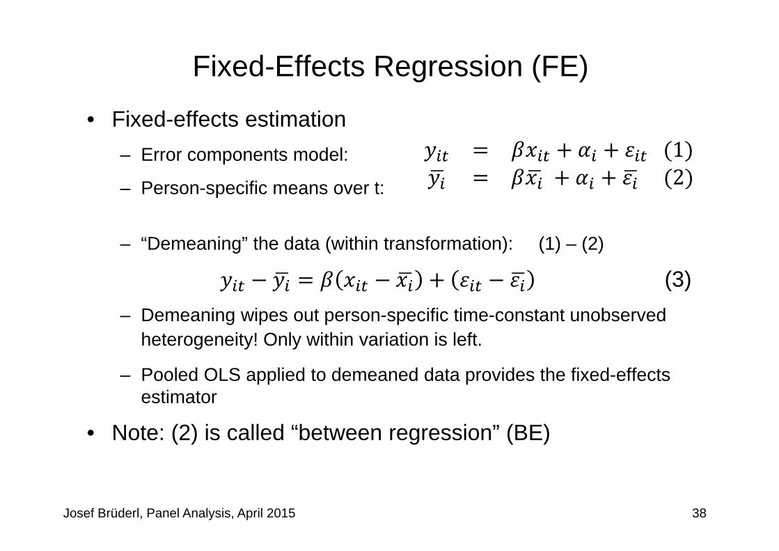
• Fixed-effects estimation– Error components model:
– Person-specific means over t:
– “Demeaning” the data (within transformation): (1) – (2)
(3)– Demeaning wipes out person-specific time-constant unobserved
heterogeneity! Only within variation is left.
– Pooled OLS applied to demeaned data provides the fixed-effects estimator
• Note: (2) is called “between regression” (BE)
38
1 2

Assumptions of FE Estimation• The FE-estimator is consistent if
E | 0forall and strict exogeneity assumption- Intuition: otherwise and would be correlated
– However, because is not in the demeaned equation, E | 0 is no longer required for consistency
- FE identifies the causal effect under weaker assumptions Time-constant unobserved heterogeneity is allowedOnly time-varying unobserved heterogeneity must not be
Josef Brüderl, Panel Analysis, April 2015 39
wagemarriage
cosmeticsurgeryintelligenceattractivity
wagemarriage
cosmeticsurgery
within transformation
demeaned data: , etc.
Josef Brüderl, Panel Analysis, April 2015
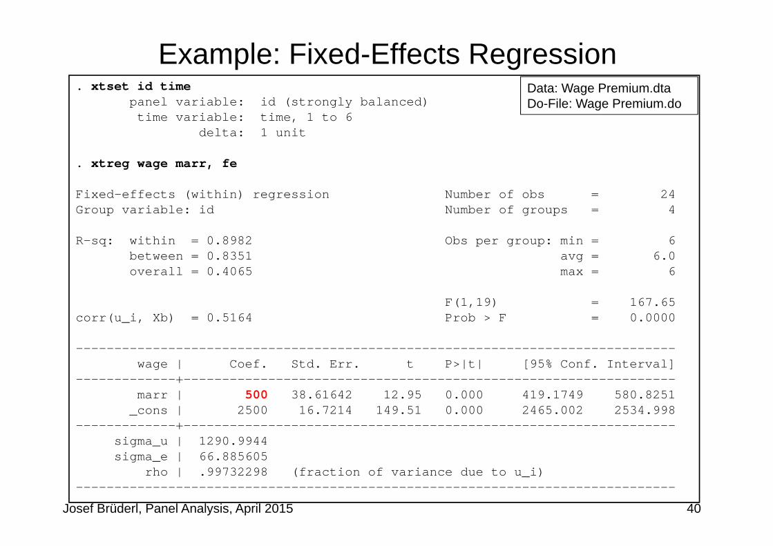
Example: Fixed-Effects Regression. xtset id time
panel variable: id (strongly balanced)time variable: time, 1 to 6
delta: 1 unit
. xtreg wage marr, fe
Fixed-effects (within) regression Number of obs = 24Group variable: id Number of groups = 4
R-sq: within = 0.8982 Obs per group: min = 6between = 0.8351 avg = 6.0overall = 0.4065 max = 6
F(1,19) = 167.65corr(u_i, Xb) = 0.5164 Prob > F = 0.0000
------------------------------------------------------------------------------wage | Coef. Std. Err. t P>|t| [95% Conf. Interval]
-------------+----------------------------------------------------------------marr | 500 38.61642 12.95 0.000 419.1749 580.8251
_cons | 2500 16.7214 149.51 0.000 2465.002 2534.998-------------+----------------------------------------------------------------
sigma_u | 1290.9944sigma_e | 66.885605
rho | .99732298 (fraction of variance due to u_i)------------------------------------------------------------------------------
40
Data: Wage Premium.dtaDo-File: Wage Premium.do

Interpreting the FE Output• The FE model succeeds in identifying the true causal effect!
– Marriage increases the wage by 500 €– The effect is significant (judged by the t-value or the p-value)– A constant is reported, since Stata adds back the wage mean for
0, which is 2500 here– Model fit can be judged by the within 2 as usual (referring to (3))
- 90% of the within wage variation is explained by marital status change- The between and overall 2 refer to different models and are not useful
here– Variance of the error components
- sigma_u is the estimated standard deviation of - sigma_e is the estimated standard deviation of
• Further details: Andreß et al. (2013: 4.1.2.1)
Josef Brüderl, Panel Analysis, April 2015 41

Josef Brüderl, Panel Analysis, April 2015
-400
-300
-200
-100
0
100
200
300
400
dem
eane
d(w
age)
-.5 0 .5demeaned(marr)
“Mechanics” of a FE-Regression
• Those, never marrying are at 0. They contribute nothing to the regression.• The slope is only determined by the wages of those marrying:
It is the difference in the mean wage before and after marriage.
42
Data: Wage Premium.dtaDo-File: Wage Premium.do

010
0020
0030
0040
0050
00E
UR
O p
er m
onth
1 2 3 4 5 6Time
before marriage after marriage
FE-Regression• This is the information used by a FE-regression
Josef Brüderl, Panel Analysis, April 2015 43

Between- and Within-Variation• To identify the causal effect of
a marriage …– a between regression (BE) uses the
between variation- This is heavily affected by self-selection
of the high-wage men into treatment- The BE marriage premium is estimated
to be 4500 €!
– a within regression (FE) uses only within variation (of the treated only)- The causal effect is identified by the
deviations from the person-specific means
- The “contaminated” (Allison 2009) between variation is ignored completely
- Therefore, self-selection into treatment does not bias results
Josef Brüderl, Panel Analysis, April 2015 44
0
1000
2000
3000
4000
5000
EUR
O p
er m
onth
1 2 3 4 5 6Time
0
1000
2000
3000
4000
5000
EU
RO
per
mon
th
1 2 3 4 5 6Time

Josef Brüderl, Panel Analysis, April 2015
Equivalent FE-estimator I: LSDV
• Least-squares-dummy-variables-estimator (LSDV)• Practical only when is small• We get estimates for the
. regress wage marr ibn.id , noconstant
Source | SS df MS Number of obs = 24-------------+------------------------------ F( 5, 19) = 9052.94
Model | 202500000 5 40500000 Prob > F = 0.0000Residual | 85000 19 4473.68421 R-squared = 0.9996
-------------+------------------------------ Adj R-squared = 0.9995Total | 202585000 24 8441041.67 Root MSE = 66.886
------------------------------------------------------------------------------wage | Coef. Std. Err. t P>|t| [95% Conf. Interval]
-------------+----------------------------------------------------------------marr | 500 38.61642 12.95 0.000 419.1749 580.8251
id 1 | 1000 27.30593 36.62 0.000 942.848 1057.1522 | 2000 27.30593 73.24 0.000 1942.848 2057.1523 | 3000 33.4428 89.71 0.000 2930.003 3069.9974 | 4000 33.4428 119.61 0.000 3930.003 4069.997
------------------------------------------------------------------------------
45
Data: Wage Premium.dtaDo-File: Wage Premium.do

0
1000
2000
3000
4000
5000
EU
RO
per
mon
th
0 1marriage
Josef Brüderl, Panel Analysis, April 2015
Equivalent FE-estimator II: Individual Slope Regression
• Estimate a separate regression for every man marrying (blue)– In our data the slopes are equal: +500 for both men
• The FE estimator is the (weighted) mean of the individual slopes– On average this gives +500, identical to the FE estimator from above
46
Data: Wage Premium.dtaDo-File: Wage Premium.do

Chapter III: An Intuitive Introduction to Linear Panel
Regression
Josef BrüderlApplied Panel Data Analysis
Section: Within Estimation With Control Group

010
0020
0030
0040
0050
00E
UR
O p
er m
onth
1 2 3 4 5 6Time
before marriage after marriage
Josef Brüderl, Panel Analysis, April 2015
Problem: No Control Group
Modified Data:
“wage3” is a new wage variable
Now, there is a periodeffect: general wageincrease at 4.
In addition, there is no causal effect of a marriage!
But there is still selectivity.
48
Data: Wage Premium.dtaDo-File: Wage Premium.do
• So far we used estimation strategies without control group- This works only, if there is temporal homogeneity
(as is the case with our data)- It does not work, however, if there are period and/or age effects

Josef Brüderl, Panel Analysis, April 2015
Problem: No Control Group
• FE-regression yields the wrong answer– Reason is that FE does not use the control group information – This is generally true: groups where does not change contribute
nothing to the FE-estimator- Note that Stata reports the in the data, not the used for FE-estimation!
. xtreg wage3 marr, fe
Fixed-effects (within) regression Number of obs = 24Group variable: id Number of groups = 4
R-sq: within = 0.4732 Obs per group: min = 6between = 0.8000 avg = 6.0overall = 0.3958 max = 6
F(1,19) = 17.07Prob > F = 0.0006
------------------------------------------------------------------------------wage3 | Coef. Std. Err. t P>|t| [95% Conf. Interval]
-------------+----------------------------------------------------------------marr | 500 121.0336 4.13 0.001 246.6738 753.3262
_cons | 2625 52.40907 50.09 0.000 2515.307 2734.693-------------+----------------------------------------------------------------
49
Data: Wage Premium.dtaDo-File: Wage Premium.do

Josef Brüderl, Panel Analysis, April 2015
Solution: Two-way FE-Regression• Including time fixed-effects ( 1 period dummies )
– Now also the control group information is used for estimating the period effects
. xtreg wage3 marr i.time , fe
------------------------------------------------------------------------------wage3 | Coef. Std. Err. t P>|t| [95% Conf. Interval]
-------------+----------------------------------------------------------------marr | -4.59e-13 58.24824 -0.00 1.000 -124.93 124.93
time 2 | 50 50.44445 0.99 0.338 -58.19259 158.19263 | 62.5 50.44445 1.24 0.236 -45.69259 170.69264 | 537.5 58.24824 9.23 0.000 412.57 662.435 | 562.5 58.24824 9.66 0.000 437.57 687.436 | 512.5 58.24824 8.80 0.000 387.57 637.43
|_cons | 2462.5 35.66961 69.04 0.000 2385.996 2539.004
-------------+----------------------------------------------------------------
One should always model time in a FE-regression!(via age and/or period effects, see chap. VI)
50
Data: Wage Premium.dtaDo-File: Wage Premium.do
Chapter IV: The Basics of Linear Panel Regression
Josef BrüderlApplied Panel Data Analysis
Section: Linear Panel ModelsMore details on the statistics can be found in Brüderl/Ludwig (2015)

A Note on the Exogeneity Assumptions• In this section we generalize to a multivariate regression
– Now we have regressors , … , . is the 1 vector (row vector) of the observed covariates of a person.
– is the corresponding 1 vector (column vector) of parameters to be estimated (regression coefficients)
– Now the exogeneity assumptions in conditional mean formulation areE | 0
E | , 0- The error terms must be independent from all regressors- For statistical inference, as well as efficiency properties of estimators these
(strong) exogeneity assumptions must hold (Wooldridge, 2010: 288)– For consistency, however, also weaker assumptions of linear
independence sufficeCov , ECov , E
- In the following we will use the exogeneity assumptions in this weaker form
Josef Brüderl, Panel Analysis, April 2015 52

POLS Estimation• We start from a multivariate error components model
– From the perspective of non-experimental research, the most critical assumptions are exogeneity assumptions on the error terms: both error terms have to be uncorrelated with the regressors
random-effects assumptioncontemporaneous exogeneity assumption
– Contemporaneous exogeneity requires that idiosyncratic errors are not systematically related to the regressors. This assumption is often reasonable.
– The random-effects assumption, however, often will be violated because slow-to-change, hard-to-measure traits that are correlated with the regressors are ubiquitous (Firebaugh et al. 2013)
- E.g., cognitive and non-cognitive ability, genetic disposition, personality, social milieu, peer group characteristics
– If the random-effects assumption fails, estimates of will be biased (omitted variable bias) (unobserved heterogeneity bias)
Josef Brüderl, Panel Analysis, April 2015 53

FE Estimation• FE wipes out person-specific time-constant unobservables
(fixed-effects) by applying the within transformation– The model (including time-constant variables )
– “Demeaning” the data (within transformation):
– Now the have gone from the equation, and POLS will provide consistent estimates of , if the assumptions on the next slide hold
– Note 1: By the within transformation also all time-constant variableshave been eliminated. With FE it is not possible to estimate their
effects .
– Note 2: The term “fixed-effects” comes from the older literature, where the are seen as unit-specific parameters to be estimated for each unit (LSDV). The newer literature sees the also as random variables (Wooldridge, 2010: 285f).
Josef Brüderl, Panel Analysis, April 2015 54

FE Assumptions• No assumption on person-specific time-constant unobserved
heterogeneity is needed – We no longer need the random-effects assumption– Instead, the “fixed-effects assumption” allows for arbitrary correlation
between and – The FE estimator is consistent even if
• For consistent estimates we need, forall , 1, … , strict exogeneity assumption
– Covariates in each time period are uncorrelated with the idiosyncratic error in each time period
– For consistency of estimates strict exogeneity is essential. Therefore, it is very important to discuss the plausibility of this assumption in every FE application [see Chapter X]
• Further FE assumptions (Wooldridge, 2010: 300 ff)– Full rank of the matrix of the demeaned regressors (no multicollinearity)– Idiosyncratic errors have constant variance across t (homoskedasticity)– Idiosyncratic errors are serially uncorrelated (no autocorrelation)
Josef Brüderl, Panel Analysis, April 2015 55

Other Within Estimators• Least-squares-dummy-variables (LSDV)
– POLS model, including a dummy for each person– Equivalent with FE – However, computationally impractical with large
• First-differences (FD)– FE and FD are equivalent for 2. However for longer panels they
will differ. FD is less efficient than FE.– However, instead of „strict exogeneity“ only „sequential exogeneity“! – Wooldridge (2010: 321ff) gives an extended discussion of the pros
and cons of FD and FE. He finally favors FE (as does the literature).
• Difference-in-differences (DiD)– DiD implements a before-after comparison with control group
- DiD is intuitively appealing (and for 2 equivalent to FD and FE)- For 2 and with controls DiD differs, however, from FD and FE
– Therefore, generally DiD is not recommended for individual panel data (more on DiD in Chapter VII)
Josef Brüderl, Panel Analysis, April 2015 56

Josef Brüderl, Panel Analysis, April 2015
Statistical Inference With Panel Data• With panel data the idiosyncratic errors are potentially
– Heteroskedastic (i.e., nonconstant variance)– Autocorrelated (i.e., serial correlation in : 1, … , )
• Ignoring this leads to under-estimated S.E.s– POLS ignores the panel structure completely– FE assumes equi-correlated errors over , which is a quite unrealistic
error structure
• Solution I: Assume a more realistic error structure– In Stata with
- xtgee: generalized linear models with unit-specific correlation structure- xtregar: panel regression with first-order autoregressive error term
– Drawback: results heavily depend on the assumptions made– And: xtgee estimates pooled models!
- Thus, the S.E.s might be improved. However, the effect estimates are probably severely biased!
57

Panel-Robust S.E.s• Solution II: panel-robust S.E.s
– An extension of the Huber-White sandwich estimator- They correct for arbitrary serial correlation and heteroskedasticity- For formulas see Brüderl/Ludwig (2015: 334)- In Stata via vce(cluster id)
– However, panel-robust S.E.s are also biased in finite samples- Sometimes they are even smaller than conventional S.E.s- But: “Your standard errors probably won’t be quite right, but they
rarely are. Avoid embarrassment by being your own best skeptic, and especially, DON’T PANIC!” (Angrist/Pischke, 2009: 327)
- The major task with non-experimental data is to get the (causal) effect estimates right, a minor task is to get the S.E.s right!
• Solution III: (panel) bootstrap S.E.s– In Stata via vce(bootstrap)
- Draw many samples over (with replacement) (size )- Calculate the coefficient estimate- Compute the variance of all these estimates (50 replications)
Josef Brüderl, Panel Analysis, April 2015 58
Josef Brüderl, Panel Analysis, April 2015
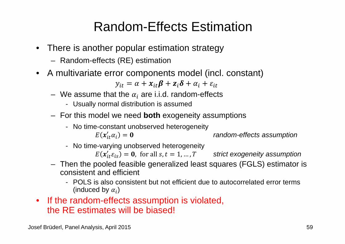
Random-Effects Estimation• There is another popular estimation strategy
– Random-effects (RE) estimation
• A multivariate error components model (incl. constant)
– We assume that the are i.i.d. random-effects - Usually normal distribution is assumed
– For this model we need both exogeneity assumptions- No time-constant unobserved heterogeneity
random-effects assumption- No time-varying unobserved heterogeneity
, forall , 1, … , strict exogeneity assumption– Then the pooled feasible generalized least squares (FGLS) estimator is
consistent and efficient- POLS is also consistent but not efficient due to autocorrelated error terms
(induced by )• If the random-effects assumption is violated,
the RE estimates will be biased!
59

Josef Brüderl, Panel Analysis, April 2015
Random-Effects Estimation• Alternatively RE can be obtained via transformed data
– RE is obtained by applying POLS to the quasi-demeaned data1 1 1 (4)
– Where 1
– This shows that the RE estimator mixes between and within estimators. The two extreme cases are‐ 1: FE estimator (e.g., → ∞, large)‐ 0: POLS
– RE estimates are between POLS and FE (in the bivariate case)
• As can be seen, with RE we also get estimates of the effects of time-constant regressors ( )
60

Josef Brüderl, Panel Analysis, April 2015
Example: Random-Effects Regression. xtreg wage marr, re theta
Random-effects GLS regression Number of obs = 24Group variable: id Number of groups = 4
R-sq: within = 0.8982 Obs per group: min = 6between = 0.8351 avg = 6.0overall = 0.4065 max = 6
Random effects u_i ~ Gaussian Wald chi2(1) = 128.82corr(u_i, X) = 0 (assumed) Prob > chi2 = 0.0000theta = .96138358
------------------------------------------------------------------------------wage | Coef. Std. Err. z P>|z| [95% Conf. Interval]
-------------+----------------------------------------------------------------marr | 502.9802 44.31525 11.35 0.000 416.1239 589.8365
_cons | 2499.255 406.0315 6.16 0.000 1703.448 3295.062-------------+----------------------------------------------------------------
sigma_u | 706.57936sigma_e | 66.885605
rho | .99111885 (fraction of variance due to u_i)------------------------------------------------------------------------------
61
Data: Wage Premium.dtaDo-File: Wage Premium.do

Interpreting the RE Output• The RE model does not succeed in identifying the true
causal effect!– Marriage increases the wage by 503 €
- The reason for the bias is that in our data the random-effects assumption is violated
- However, the bias is low, because 0.96- This is because is so large in our data
– The effect is significant (judged by the t-value or the p-value)– The “relevant” 2 would refer to (4) and is not estimable
- Model fit can “approximately” be judged by the within 2 where the RE-estimates are plugged into (3)
- Approximately 90% of the within wage variation is explained by marital status change
Josef Brüderl, Panel Analysis, April 2015 62
Chapter IV: The Basics of Linear Panel Regression
Josef BrüderlApplied Panel Data Analysis
Section: Fixed- or Random-Effects?

When Does a Within Approach Apply?• Within estimators cannot estimate
the effects of time-constant variables – E.g., sex, nationality, social origin, birth cohort, etc.– This reflects the fact that panel data do not help to identify the
causal effect of time-constant variables- One can even discuss, whether the concept of “causality” makes
sense with time-constant variables!
• The "within logic" applies only with time-varying variables– Something has to “happen”:
Only then a before-after comparison is possible Analyzing the effects of events
– Such questions are the main strength of panel data and within methodology
– [Event variables can not only be categorical, but also metric]
Josef Brüderl, Panel Analysis, April 2015 64

The Primary Advantage of Panel Data• Panel data and within estimation allow to identify causal
effects under weaker assumptions: time-constant unobserved heterogeneity does not bias estimates– “In many applications the whole point of using panel data is to
allow for to be arbitrarily correlated with the . A fixed effects analysis achieves this purpose explicitly.” (Wooldridge, 2010: 300)
– “The DiD, fixed effects, and first difference estimators (within estimators) offer researchers the capacity to dispense with the random effects assumption and still obtain unbiased and consistent estimates when unit effects [ ] are arbitrarily correlated with measured explanatory variables. This is widely regarded as the primary advantage of panel data.” (Halaby, 2004: 516)
Josef Brüderl, Panel Analysis, April 2015 65

Sociologists Often Use RE Models• RE is biased by time-constant unobserved heterogeneity
– Since time-constant unobserved heterogeneity is ubiquitous in non-experimental social research, RE estimates generally will be biased
– So why would anybody want to use RE models?
• Unfortunately, sociologist often use RE models– Halaby (2004) identifies 31 papers appearing in ASR and AJS
between 1990 and 2003 that use panel data for causal analysis. 15 out of these used RE only
– Giesselmann/Windzio (2014) identify 10 papers appearing in ZfSand KZfSS between 2000 and 2009 that use panel data for causal analysis. 3 out of these used RE only
• Two arguments in favor of RE are often brought forward– RE allows for estimating effects of time-constant regressors– RE is more efficient than FE, if
Josef Brüderl, Panel Analysis, April 2015 66

Effects of Time-Constant Regressors• Often it is argued that wiping out all time-constant regressors
is a shortcoming of FE estimation– However, wiping out all time-constant regressors is not a
shortcoming of FE. In fact it is a major strength, because alongside also all time-constant unobservables are eliminated
• The shortcoming is with a style of data analysis that by default throws all kinds of controls into a regression (“kitchen-sink-approach”)– Using the RE estimator only to report effects of sex, race, etc. is
risking to throw away the big advantage of panel data– Instead of a thoughtless kitchen-sink-approach we should carefully
think about the identification of a single causal effect (X centering)• If one has substantive interest in the effect of a time-
constant regressor, one should use group specific growth curves, instead of a simple RE model (see Chapter VI)
Josef Brüderl, Panel Analysis, April 2015 67

0
.1
.2
.3
.4
.5
.6
.7
.8
dens
ity
-4 -3 -2 -1 0 1 2 3 4
regression estimate
FE estimateRE estimate
Josef Brüderl, Panel Analysis, April 2015
Bias versus Efficiency• Sometimes it is argued, that a biased but efficient estimate (RE)
might be preferable to an unbiased but less efficient estimate (FE)– This argument is only sound, if the bias is small– However, RE is more efficient because it also uses the endogenous
between variation. Generally, this is not a good idea, because this will produce a large bias.
“true” value: β = 0
68
A thought experiment to illustrate the point

| (b) (B) (b-B) sqrt(diag(V_b-V_B))| FE RE Difference S.E.
-------------+----------------------------------------------------------------marr | 500 502.9802 -2.980234 1.210069
------------------------------------------------------------------------------b = consistent under Ho and Ha; obtained from xtregB = inconsistent under Ha, efficient under Ho; obtained from xtreg
Test: Ho: difference in coefficients not systematic
chi2(1) = (b-B)'[(V_b-V_B)^(-1)](b-B) = 6.07Prob>chi2 = 0.0138
Josef Brüderl, Panel Analysis, April 2015
Testing whether RE or FE: Hausman Test• Use RE models only, if a Hausman test says „it is ok“
– The intuition: the FE estimates ( ) are consistent; If the RE estimates ( ) do not differ too much, one can use RE regression
H ∶
~ – If you are not able to reject H0, then you can use RE
69
Data: Wage Premium.dtaDo-File: Wage Premium.do

Chapter V: A Real Data Example:
Marriage and Happiness
Josef BrüderlApplied Panel Data Analysis
Section: Preparing Panel Data

Josef Brüderl, Panel Analysis, April 2015
Example: Does Marriage Make Happy?• In the following we will use a real data example• The goal is to estimate the causal effect of (first) marriage
on happiness– More exactly: life satisfaction (or: subjective well-being)
• Data: SOEP 1984-2009 (v26)– The data set contains repeated measures for the same persons on
the following variables: - Life satisfaction, marriage, years married, household income, age, sex,
year of interview
71

Josef Brüderl, Panel Analysis, April 2015
marriage
marriage
Panel
The Problem again is Self-Selection: Happy People are More Likely to Get Married
See also: Stutzer/Frey (2005)
1
2
3
4
5
6
7
1 2 3
year
happ
ines
sCross-Section
72
Dilbert also is aware of the problem

Josef Brüderl, Panel Analysis, April 2015
Preparing the Data for Panel Analysis• Retrieving the data: “Happiness 1 Retrieval.do”
- First “happy” is retrieved from $P, GPOST, and $PAGE17- The covariates needed are retrieved from $PEQUIV
• Preparing the data: “Happiness 2 DataPrep.do”- Variables are recoded and time-varying covariate “marry” is built- The estimation sample is selected
• Analyzing the data: “Happiness 3/4/5 Regressions.do”- Data file: “Happiness2.dta”- The lecture-package includes an anonymized version of these data
(50% sample). Therefore, results are very similar, but not identical to the ones reported in the lecture.
73
marry: age: loghhinc:marriage dummy age in years natural logarithm of
annual post-government household income
yrsmarried: woman:years since marriage dummy for women

Josef Brüderl, Panel Analysis, April 2015
Defining the Estimation Sample• How to define the estimation sample?
– Practically very important, but (almost) nothing can be found in literature– One should include only those, who potentially can change from
the state of not-treated to treated (Sobel 2012)- Only those persons, who experience treatment during the observation
period provide within information and identify the treatment effect- Include also the never-treated persons as a control group- The already-treated might bias the estimation of the treatment effect
- The already-treated might improve the precision of the estimated age effect. However, if the treatment effect varies over time, then the age effect of the already-treated might be distorted.
• For our example, we restrict the estimation sample accordingly– Only persons are included, who were single when first observed
(persons married when first observed, are discarded altogether!)– Person-years after marital separation are excluded– Persons with only one person-year are excluded
• Deleting so many observations differs markedly from what one is used from cross-sectional data analysis!– We end up with only 29% of all available person-years
74

Time-Ordering of Events• Causality requires that the cause precedes the effect
– Panel data help to identify the time-ordering of treatment and outcome
– This has to be taken into regard when preparing the data
• Example: binary treatment (absorbing)– An event happens between wave 1 and
, … , 0, … , 1
– Outcomes have to be measured accordingly, … , measuredbeforeevent, … , measuredafterevent
• Happiness example– All variables measured at time of interview. Therefore, no problem
‐ 0, 1 if there was a marriage between 1 and ‐ is measured then before, and after marriage
Josef Brüderl, Panel Analysis, April 2015 75

Josef Brüderl, Panel Analysis, April 2015
How to Model a Causal Effect?• With panel data we can investigate the time path of a causal effect
• Termed “impact function” (IF) by Andreß et al. (2013)• Different impact functions can be modeled
76
Step impact functionImmediate and permanent impact
● event dummy (0,0,0,0,1,1,1)
Y
TEvent
Continuous impact functionImmediate, but transitory impact
● event dummy (0,0,0,0,1,1,1)● linear event time (0,0,0,0,0,1,2)● quadratic event time (0,0,0,0,0,1,4)
Y
TEventDummy impact functionArbitrary impact (including anticipation effect)
● dummy event time− -1 dummy (0,0,0,1,0,0,0)− 0 dummy (0,0,0,0,1,0,0)− 1 dummy (0,0,0,0,0,1,0)− 2 dummy (0,0,0,0,0,0,1)
Y
TEvent

Presenting Regression Results Graphically• Instead of regression tables with many numbers, it is helpful
to present the important results graphically (Bauer, 2015)• Basically there are three types of graphs available
– Plotting average marginal effects (AME) (effect plot)- How, does a one unit change in X affect Y? (marginal effect for
continuous variables, discrete change for categorical variables)- Computed for each observation in the data given their respective
values on other variables. Then averaged over all observations.- For linear models these are simply the regression coefficients
– Plotting the predicted values (profile plot)- What are the predicted values for Y given the values of X?
- Computed for each observation in the data and then averaged (predictive margins)
– Plotting AMEs of X conditional on values of Z (conditional effect plot)- How changes the AME of X over the values of Z?- Helpful for interaction effects and for impact functions
Josef Brüderl, Panel Analysis, April 2015 77

Chapter V: A Real Data Example:
Marriage and Happiness
Josef BrüderlApplied Panel Data Analysis
Section: Describing Panel Data
Josef Brüderl, Panel Analysis, April 2015
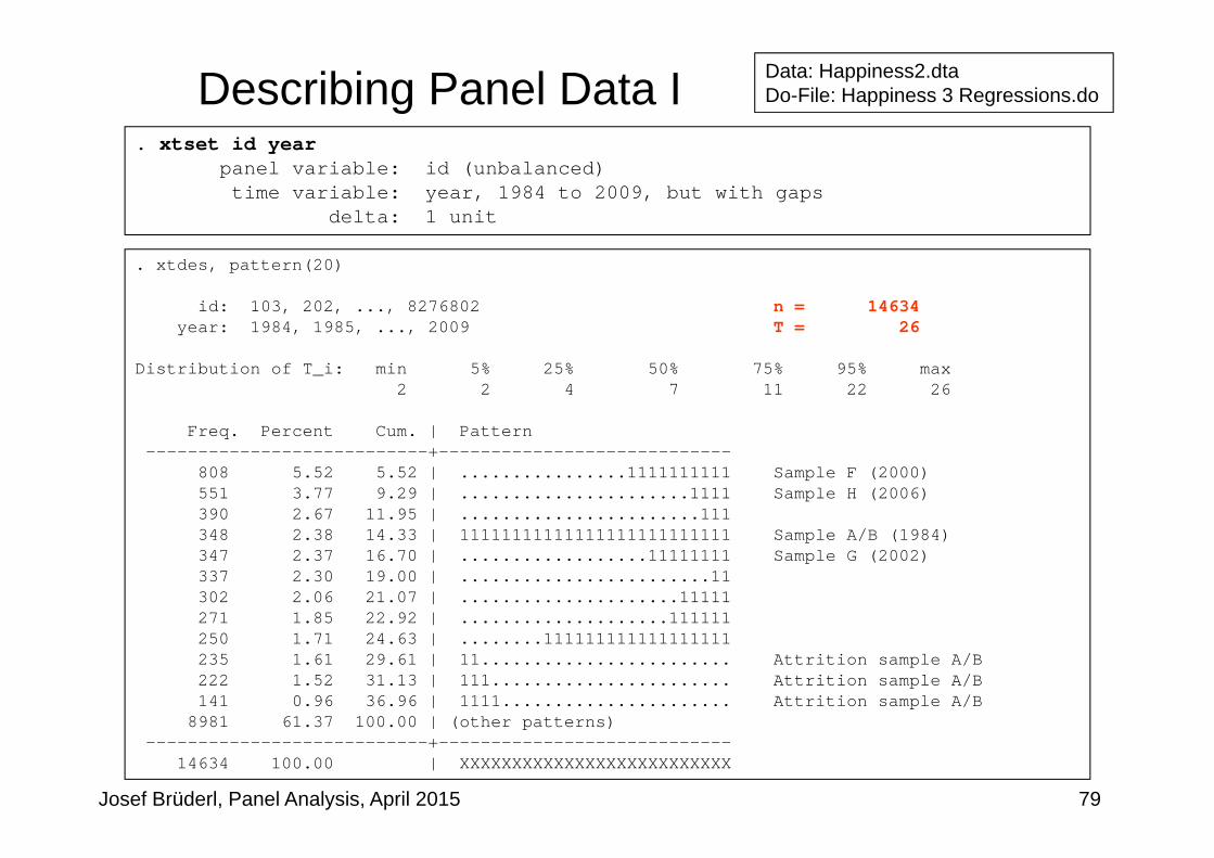
Describing Panel Data I. xtset id year
panel variable: id (unbalanced)time variable: year, 1984 to 2009, but with gaps
delta: 1 unit
. xtdes, pattern(20)
id: 103, 202, ..., 8276802 n = 14634year: 1984, 1985, ..., 2009 T = 26
Distribution of T_i: min 5% 25% 50% 75% 95% max2 2 4 7 11 22 26
Freq. Percent Cum. | Pattern---------------------------+----------------------------
808 5.52 5.52 | ................1111111111 Sample F (2000)551 3.77 9.29 | ......................1111 Sample H (2006)390 2.67 11.95 | .......................111348 2.38 14.33 | 11111111111111111111111111 Sample A/B (1984)347 2.37 16.70 | ..................11111111 Sample G (2002)337 2.30 19.00 | ........................11302 2.06 21.07 | .....................11111271 1.85 22.92 | ....................111111250 1.71 24.63 | ........111111111111111111235 1.61 29.61 | 11........................ Attrition sample A/B222 1.52 31.13 | 111....................... Attrition sample A/B141 0.96 36.96 | 1111...................... Attrition sample A/B
8981 61.37 100.00 | (other patterns)---------------------------+----------------------------
14634 100.00 | XXXXXXXXXXXXXXXXXXXXXXXXXX
79
Data: Happiness2.dtaDo-File: Happiness 3 Regressions.do

Josef Brüderl, Panel Analysis, April 2015
Describing Panel Data II. xttrans marry , freq
| marry (t+1)marry (t) | 0 1 | Total
-----------+----------------------+----------0 | 79,209 3,793 | 83,002
| 95.43 4.57 | 100.00 -----------+----------------------+----------
1 | 0 24,283 | 24,283 | 0.00 100.00 | 100.00
-----------+----------------------+----------Total | 79,209 28,076 | 107,285
. xtsum marry age loghhinc woman
Variable | Mean Std. Dev. Min Max | Observations-----------------+--------------------------------------------+----------------marry overall | .230284 .4210163 0 1 | N = 121919
between | .2694525 0 .9615385 | n = 14634within | .2671083 -.7312544 1.191823 | T-bar = 8.33121
| |age overall | 29.27678 11.12508 16 97 | N = 121919
between | 10.47358 16.5 96.5 | n = 14634within | 4.310836 13.90178 45.19345 | T-bar = 8.33121
| |loghhinc overall | 10.21187 .6562057 0 14.16139 | N = 121919
between | .5664285 6.034016 13.2728 | n = 14634within | .4252418 2.134135 12.9504 | T-bar = 8.33121
| |woman overall | .467179 .4989237 0 1 | N = 121919
between | .4992656 0 1 | n = 14634within | 0 .467179 .467179 | T-bar = 8.33121
Is there enough within variation?
80
Data: Happiness2.dtaDo-File: Happiness 3 Regressions.do

Chapter V:
Josef BrüderlApplied Panel Data Analysis
Section: The Results- Panel-robust S.E.s- Step impact function- Continuous impact function- Dummy impact function

Josef Brüderl, Panel Analysis, April 2015
Panel-Robust S.E.s--------------------------------------------------
| FE FE FE S.E.| conventional panel-robust bootstrap
-------------+------------------------------------marry | 0.1668 0.1668 0.1668
| 0.0168 0.0226 0.0189 | 9.9503 7.3692 8.8254
age | -0.0413 -0.0413 -0.0413 | 0.0010 0.0017 0.0017 | -39.3197 -23.9552 -23.6374
loghhinc | 0.1245 0.1245 0.1245 | 0.0093 0.0123 0.0128 | 13.4180 10.1600 9.7087
--------------------------------------------------legend: b/se/t
Conventional S.E.s are too small.Panel-robust S.E.s are close to the bootstrap S.E.s.Obviously, with over 14,000 clusters asymptotics works well. In the following we will always use panel-robust S.E.s!
82
Data: Happiness2.dtaDo-File: Happiness 3 Regressions.do

Josef Brüderl, Panel Analysis, April 2015
Comparing Results From Step IF-------------------------------------------------------------------------------Variable | BE POLS RE FE FD ---------+---------------------------------------------------------------------
marry | 0.52*** 0.34*** 0.20*** 0.17*** 0.14***loghhinc | 0.50*** 0.38*** 0.20*** 0.12*** 0.05**
woman | 0.03 0.03 0.03 (omitted) (omitted)---------+---------------------------------------------------------------------
N | 14634 121919 121919 121919 104671 N_clust | 14634 14634 14634 14511 -------------------------------------------------------------------------------
legend: * p<0.05; ** p<0.01; *** p<0.001
Marriage effect: Heavily biased upwards by BE and POLSRE is still biased upwards (median theta is 0.58)FD too low due to anticipation (see below)
Income effect: Heavily biased upwards by BE, POLS, and RE; unobservables affecting income and happiness: happy people earn more money
Sex effect: Time-constant variable not estimable with FE and FD
83
Data: Happiness2.dtaDo-File: Happiness 3 Regressions.do
FD: Due to gaps in the data we loose some groups (clusters) and observations.
All models control for age and cohort (see Chapter VI for details)

marriage
ln(HHincome)
woman
-.1 0 .1 .2 .3 .4
Effect on happiness
POLS RE FE
Regression Coefficients with 95% CIs
Comparing Estimation Results Graphically• Comparing regression coefficients across models is much more
effective, if done graphically– The “coefplot” package (Jann 2014) is here very helpful in this respect
Josef Brüderl, Panel Analysis, April 2015 84
ssc install coefplot, replace // Install "coefplot" package (Jann 2014)coefplot POLS RE FE, keep(marry loghhinc woman) xline(0)

Why Do We Need a Control Group?
• Estimation sample: (1) only those who married, (2) plus control group– Marriage effect is not affected, because the control group contributes nothing to the FE estimate– S.E.s differ al little, because the d.f.s are different
• (3) and (4) include age as control– The marriage effect in (1) and (2) is obviously heavily biased
- The reason is that with increasing age there is a happiness decline (more details in Chap. VI)- Lesson 1: It is important to control for time-varying confounders in FE models
– In (3) the age effect is estimated only with those who married. It is too low, as can be seen in the full sample (4) including the control group
- This also affects the marriage effect, that is too low in (3)- Lesson 2: We see that it is important to include a control group to get the estimates of the
control variables right
Josef Brüderl, Panel Analysis, April 2015 85
------------------------------------------------------FE estimates | (1) (2) (3) (4) -------------+----------------------------------------
marry | -0.139 -0.139 0.136 0.186 | 0.0139 0.0144 0.0186 0.0167
age | -0.033 -0.039 | 0.0015 0.0010
-------------+----------------------------------------N | 49235 121919 49235 121919
N_clust | 3793 14634 3793 14634------------------------------------------------------
legend: b/se

Josef Brüderl, Panel Analysis, April 2015
Deciding Between FE and RE: Hausman Test. xtreg happy marry age loghhinc i.cohort, re. est store RE. xtreg happy marry age loghhinc, fe. est store FE. hausman FE RE, sigmamore
---- Coefficients ----| (b) (B) (b-B) sqrt(diag(V_b-V_B))| FE RE Difference S.E.
-------------+----------------------------------------------------------------marry | .1667519 .1962653 -.0295134 .0068511
age | -.0412592 -.040121 -.0011383 .0004667loghhinc | .1245142 .1956244 -.0711102 .0039792
------------------------------------------------------------------------------b = consistent under Ho and Ha; obtained from xtreg
B = inconsistent under Ha, efficient under Ho; obtained from xtreg
Test: Ho: difference in coefficients not systematic
chi2(3) = (b-B)'[(V_b-V_B)^(-1)](b-B)= 544.31
Prob>chi2 = 0.0000
use the FE model
86
Data: Happiness2.dtaDo-File: Happiness 3 Regressions.do

Josef Brüderl, Panel Analysis, April 2015
Results of a FE Model with Continuous IF. xtreg happy i.marry c.yrsmarried##c.yrsmarried age loghhinc, fe vce(cluster id)
Fixed-effects (within) regression Number of obs = 121919Group variable: id Number of groups = 14634
R-sq: within = 0.0162 Obs per group: min = 2between = 0.0221 avg = 8.3overall = 0.0152 max = 26
F(5,14633) = 144.05corr(u_i, Xb) = -0.1808 Prob > F = 0.0000
(Std. Err. adjusted for 14634 clusters in id)-------------------------------------------------------------------------------------------
| Robusthappy | Coef. Std. Err. t P>|t| [95% Conf. Interval]
--------------------------+----------------------------------------------------------------marry | 0.2413 0.0231 10.47 0.000 0.1961 0.2865
yrsmarried | -0.0411 0.0065 -6.29 0.000 -0.0539 -0.0283c.yrsmarried#c.yrsmarried | 0.0017 0.0004 4.71 0.000 0.0010 0.0024
age | -0.0372 0.0021 -17.33 0.000 -0.0415 -0.0330loghhinc | 0.1306 0.0124 10.57 0.000 0.1064 0.1549
_cons | 6.8787 0.1360 50.57 0.000 6.6121 7.1453--------------------------+----------------------------------------------------------------
sigma_u | 1.2861966sigma_e | 1.3325279
rho | .48231322 (fraction of variance due to u_i)-------------------------------------------------------------------------------------------
87
Data: Happiness2.dtaDo-File: Happiness 3 Regressions.do

marriage
yrsmarried
yrsmarried # yrsmarried
age
ln(HHincome)
-0.10 -0.05 0.00 0.05 0.10 0.15 0.20 0.25 0.30
Effect on happiness
Regression Coefficients with 95% CIs
Coefficient Plot
Josef Brüderl, Panel Analysis, April 2015 88
coefplot, drop(_cons) xline(0)

-0.3
-0.2
-0.1
0.0
0.1
0.2
0.3
0.4
0.5
Cha
nge
in h
appi
ness
0 1 2 3 4 5 6 7 8 9 10 11 12 13 14 15
Years since marriage
95%-CI
Josef Brüderl, Panel Analysis, April 2015
Impact Function of Marriage (Conditional Effect Plot)
89
• Of central interest: time path of the marginal marriage effect – Change in happiness due to a marriage ( ) over yrsmarried ( )
∗ ∗
What is the reference point?• Average happiness
of all pyrs before marriage
• Important point: only of those, who eventually marry. Not of the always singles
• After all this is a within estimator!

-0.3
-0.2
-0.1
0.0
0.1
0.2
0.3
0.4
0.5
Cha
nge
in h
appi
ness
0 1 2 3 4 5 6 7 8 9 10 11 12 13 14 15
Years since marriage
POLS RE FE
Conditional effect of marriage estimated by POLS, RE, and FE
Comparing Models
90
• Comparing the conditional marriage effect over models– We see that POLS heavily over-estimates the marriage effect
- Due to self-selection– RE slightly over-estimates the marriage effect
- RE works quite well with these data (probably due to the long panels)
Josef Brüderl, Panel Analysis, April 2015

Dummy Impact Function• A flexible way to model the causal effect is by event time dummies
– For this, we have to construct an “event centered” time scale (ym)-1 all years before marriage (ref. group)0 the year of marriage1 first year after marriage…15 15th+ year after marriage
- Be careful in 0 year: event must have happened before outcome is measured!
- We collapse the dummies 15 - max due to low case numbers– The event time dummies are easily included in a regression model
via factor notation (i.ym) [0-dummy, 1-dummy, …, 15-dummy]– Interpretation: the within estimator compares average happiness in a
particular year with average happiness in all (!) years before marriage– This model is known in the literature as distributed fixed-effects
(Dougherty 2006)- It can also be estimated by including lags and leads of the 0-dummy (this is
often done by economists, e.g. Wooldridge 2010: chap. 10)
Josef Brüderl, Panel Analysis, April 2015 91

-0.3
-0.2
-0.1
0.0
0.1
0.2
0.3
0.4
0.5
Cha
nge
in h
appi
ness
0 1 2 3 4 5 6 7 8 9 10 11 12 13 14 15
Years since marriage
Dummy Impact Function
• The dummy modelling in general supports the results from the parametric modelling above– However, we see more details: Compared to the years before marriage
- Happiness increases by 0.31 in the year of marriage- In the first year after marriage, happiness is only higher by 0.17- Beginning with the fifth year, happiness is no longer significantly higher
Josef Brüderl, Panel Analysis, April 2015 92
Data: Happiness2.dtaDo-File: Happiness 3 Regressions.do

010
0020
0030
0040
0050
00E
URO
per
mon
th
1 2 3 4 5 6Time
How to Model a Causal Effect?• Above I argued that one should use
– Either a step event dummy: 0 before, 1 after the event– Or a full set of event time dummies
• Some argue, to use the 0-dummy only– The intuitive idea is that this variable captures the change event– However, this modeling strategy would make only sense, if the
effect is immediate and very short-lived– Example: With our fabricated
data the within estimatorcompares red circled minus green circled points
- The result is +300 €- Obviously, this is biased,
because the causal effectpersists and is therefore inthe reference group
Josef Brüderl, Panel Analysis, April 2015 93

Glücksfaktoren
Josef Brüderl, Panel Analysis, April 2015 94
Source: Deutsche Post, Glücksatlas 2012
• FE models• SOEP, 1992-2010• The most important factor is
good/bad health• Life-events (marriage,
widowhood, unemployment, divorce) are next
• Here modeled as permanent effects
• Social contacts/isolation comes next
• Age is here mis-specified (see next chapter)
• Money has relatively small effects
• „Money does not make happy“

Chapter V
Josef BrüderlApplied Panel Data Analysis
Section: Interpreting Results from Panel Regressions
– Interpreting panel regression estimates– Interpreting results from impact functions– Interpreting effects of continuous variables– Interpreting interaction effects– Effects of consecutive life course events

Interpreting Panel Regression Estimates• There is much confusion in the literature on how to
interpret results from panel regressions• Regression estimates can be interpreted in two ways
– I) Descriptive interpretation- “People who differ in X by one unit, differ in Y by ”
– II) Causal interpretation- “A one unit change in X, changes Y by ”- Sometimes called “change interpretation”
• Cross-sectional (between) regression– It would be natural to choose interpretation I).
After all that is the information provided by the data!– However, often interpretation II) is chosen.
But this is only ok, if the exogeneity assumptions hold• Within regression
– It is natural to choose interpretation II). Because within estimates are obtained by a before-after comparison.
Josef Brüderl, Panel Analysis, April 2015 96

Interpreting Panel Regression Estimates
Josef Brüderl, Panel Analysis, April 2015 97
010
0020
0030
0040
0050
00E
UR
O p
er m
onth
1 2 3 4 5 6Time
before marriage after marriage
Cross-sectional regression:Married men earn 2500 € more than unmarried men (descriptive interpretation)A marriage increases men’s wage by 2500 €(causal interpretation)
POLS regression:Men living in marriage earn 1833 € more than men living unmarried (descriptive interpretation)A marriage increases men’s wage by 1833 €(causal interpretation)
010
0020
0030
0040
0050
00E
UR
O p
er m
onth
1 2 3 4 5 6Time
before marriage after marriage
010
0020
0030
0040
0050
00E
UR
O p
er m
onth
1 2 3 4 5 6Time
before marriage after marriage
Fixed-effects regression:After marriage men earn 500 € more than before marriage (descriptive interpretation)A marriage increases men’s wage by 500 €(causal interpretation)
The descriptive interpretation is always correct.The causal interpretation is only correct, if the exogeneity assumptions hold

Confusion about Interpretation• Some authors provide confused arguments
– Andreß et al. (2013) argue that- I) is appropriate for POLS and FE (modeling the level) and that - II) only works for FD (modeling the change)- However, all models can be interpreted in levels (descriptive) or
change (causal). But only FD and FE (!) use the change information contained in panel data to answer the causal question.
– Giesselmann/Windzio (2012) term- I) “cross-sectional questions”- II) “longitudinal questions”- However, both descriptive and causal questions can be answered with
either cross-sectional or longitudinal data. But the assumptions needed to get correct answers differ.
Josef Brüderl, Panel Analysis, April 2015 98

Interpreting Results from Impact Functions• With event time dummies, the within estimator compares the outcome
in a particular year with the outcome in the reference years– For each unit separately (for sure, only for the treated)– The FE estimator is the average of these unit-specific estimates
Josef Brüderl, Panel Analysis, April 2015 99
0
1000
2000
3000
4000
5000
EU
RO
per
mon
th
1 2 3 4 5 6Time
• Example– 0.ym 500
1.ym 2502.ym 0
– The effect of 0.ym is the average wage of the red points minus the average wage of the green points (only the treated)
– The effect of 1.ym is … blue points …
– The effect of 2.ym is …orange points …
– The non-treated contribute nothing to these estimates!Data: Impact Function.dta
Do-File: Impact Function.do
0
1000
2000
3000
4000
5000
EU
RO
per
mon
th
1 2 3 4 5 6Time
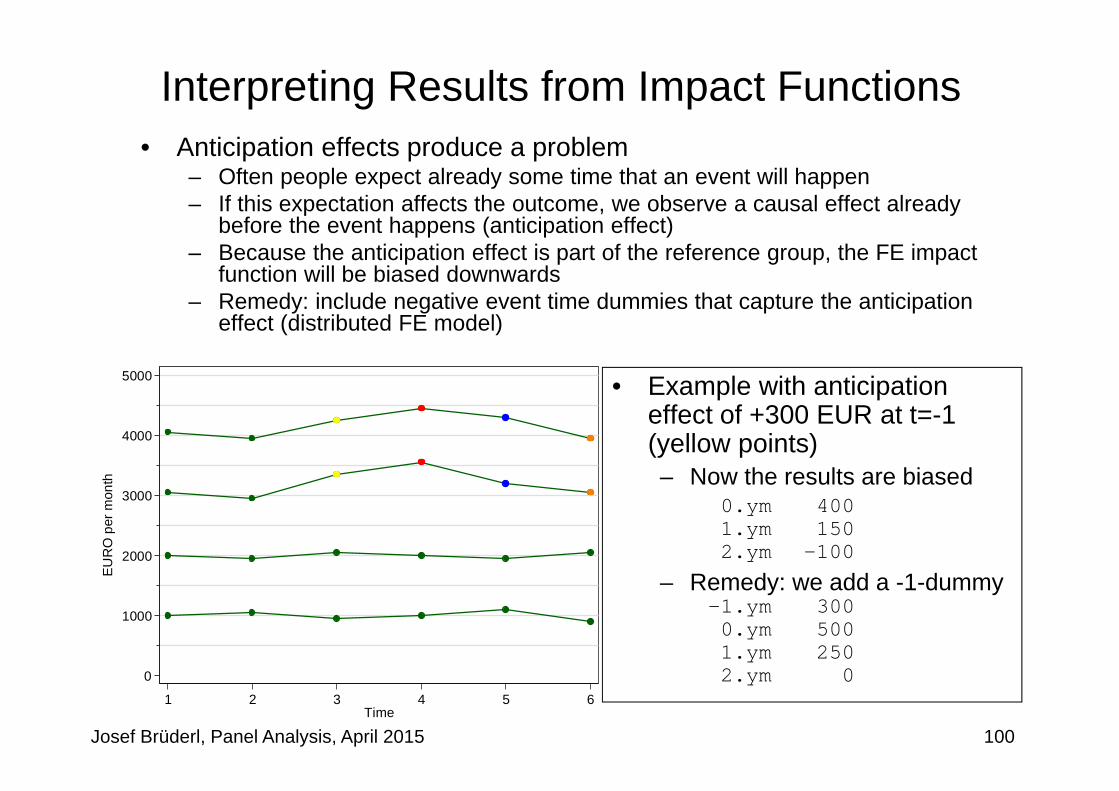
Interpreting Results from Impact Functions• Anticipation effects produce a problem
– Often people expect already some time that an event will happen– If this expectation affects the outcome, we observe a causal effect already
before the event happens (anticipation effect)– Because the anticipation effect is part of the reference group, the FE impact
function will be biased downwards– Remedy: include negative event time dummies that capture the anticipation
effect (distributed FE model)
Josef Brüderl, Panel Analysis, April 2015 100
• Example with anticipation effect of +300 EUR at t=-1 (yellow points)– Now the results are biased
0.ym 4001.ym 1502.ym -100
– Remedy: we add a -1-dummy -1.ym 3000.ym 5001.ym 2502.ym 0

-0.1
0.0
0.1
0.2
0.3
0.4
0.5
0.6
0.7
Cha
nge
in h
appi
ness
-6 -5 -4 -3 -2 -1 0 1 2 3 4 5 6 7 8 9 10 11 12 13 14 15
Years before / after marriage
Example: Marriage and Happiness• Marriage probably produces anticipation effects
– To test for these, we expand the distributed FE model up to 6
Josef Brüderl, Panel Analysis, April 2015 101
Data: Happiness2.dtaDo-File: Happiness 3 Regressions.do
We observe extremely strong anticipation effects that even change our substantive conclusions!– Reference group is up to 7 years
before marriage– With the fifth year before marriage
we observe a significant happiness increase
– In the year before marriage it is .43– In the marriage year it peaks at .54– Then it goes back to about .3– However, it never falls below the
reference level– Thus our conclusion changes
dramatically: Marriage has a long lasting effect that however can only be seen if the anticipation effect is taken into account!

Josef Brüderl, Panel Analysis, April 2015
The Effects of Life-Events on Happiness
Diener, E. et al. (2006) Beyond the Hedonic Treadmill. American Psychologist 61 (4): 305-314.
102
• With this methodology one can investigate the impact of all kinds of life-events
• Diener et al. is a classic in this respect. They use SOEP data and this graph summarizes their results (however, they use RE-modelling!)
• Their result on marriage differs from ours!?
• Unemployment has a sudden and long-lasting negative effect
• Widowhood shows anticipation (health problems of the partner) and a long-lasting negative effect
• Divorce shows anticipation (match deteriorates) but no effect on happinesso There is negative selection into
divorce

Interpreting Effects of Continuous Treatments• What does the within estimator with continuous treatments?
– Here we cannot compare to a reference group– Instead, for each individual panel a regression line is fitted. The FE
estimate is the average of these individual regression lines– Descriptive interpretation
- The outcome difference, with varying treatment– Causal interpretation
- The outcome change, with varying treatment– Again the causal interpretation hinges on weaker assumptions
- E.g., a within treatment effect results from comparing the outcome of the same person over years with different treatment values
• Example: income and happiness– We now use income in absolute terms (in 10,000 EUR)– The FE result is +0.024. The causal interpretation is that a 10 Tsd. EUR
increase in hhincome would increase happiness by .024- Obviously a very small effect- However, this is biased because of the linear modelling. In truth the income
effect is highly non-linear- This is shown on the next slide by using a categorical income variable
Josef Brüderl, Panel Analysis, April 2015 103

0-10 (ref.)
10-20
20-30
30-40
40-50
50-60
60-100
100-
0 .1 .2 .3 .4 .5
Effect of yearly HHincome (in tsd. EUR) on happiness
Example: Income and Happiness
• There is a satisfaction threshold– An income threshold after which happiness does not increase further – Wolbring et al. (2013) report that this threshold is at about 800 EUR monthly equivalence income.
According to our results it is at about 40 Tsd. gross annual HHincome• This result explains the “Easterlin paradoxon”
– Despite GDP increases in the last decades, average happiness in Western Countries did not increase
Josef Brüderl, Panel Analysis, April 2015 104

Interpreting Interaction Effects• Effect heterogeneity on a group level can be modeled by
allowing for an interaction treatment group– Whereas time-constant group effects are not identified in a within
estimation, interactions are identified– The result tells us, whether the treatment ( ) effect differs between
groups ( : 0,1 ). Note that the main effect of is not identified!– Standard interaction parametrization (adding a product term)
(the treatment effect of 0)(the difference in the treatment effect of 1)
- Stata code: i.group##i.treatment– Often it is helpful to model interactions as “nested effects”
0 1
where . 1, if. 10, else
(the treatment effect of 0)(the treatment effect of 1)
- Stata code: i.group#i.treatment– “Product term” and “nested effects” parametrization are equivalent
Josef Brüderl, Panel Analysis, April 2015 105

Example: Income Effect by Sex
• The standard interaction specification tells us that men have an income effect of +0.164
• Women’s income effect is significantly lower by -0.076
Josef Brüderl, Panel Analysis, April 2015 106
. xtreg happy marry i.woman##c.loghhinc age, fe vce(cluster id)note: 1.woman omitted because of collinearity
--------------------------------------------------------------------------------| Robust
happy | Coef. Std. Err. t P>|t| [95% Conf. Interval]---------------+----------------------------------------------------------------
marry | .1678467 .0226257 7.42 0.000 .1234976 .21219591.woman | 0 (omitted)
loghhinc | .1639288 .0177442 9.24 0.000 .1291478 .1987097woman#c.loghhinc
1 | -.0759617 .0242279 -3.14 0.002 -.1234514 -.0284721|
age | -.0413842 .0017228 -24.02 0.000 -.0447611 -.0380072_cons | 7.007378 .1270878 55.14 0.000 6.75827 7.256486
---------------+----------------------------------------------------------------
Data: Happiness2.dtaDo-File: Happiness 3 Regressions.do

Josef Brüderl, Panel Analysis, April 2015
Example: Income Effect by Sex
107
Data: Happiness2.dtaDo-File: Happiness 3 Regressions.do
• The nested effects specification is often more informative– Because it gives us both
treatment effects directly– We see that more money
makes men much more happier (+0.164) than women (+0.088)!
Men
Women
0.00 0.05 0.10 0.15 0.20
Effect of 'HHincome' on happiness
Conditional Effect Plot by Sex
• What is the reference group in a within interaction analysis?– One could have the idea that these are “all singles”, because there is no main
effect of sex in the model– However, a full interaction model provides the same estimates, as separate
regressions for men and women– This means that the respective reference group are “single men” and “single
women” (as it should be)
Josef Brüderl, Panel Analysis, April 2015
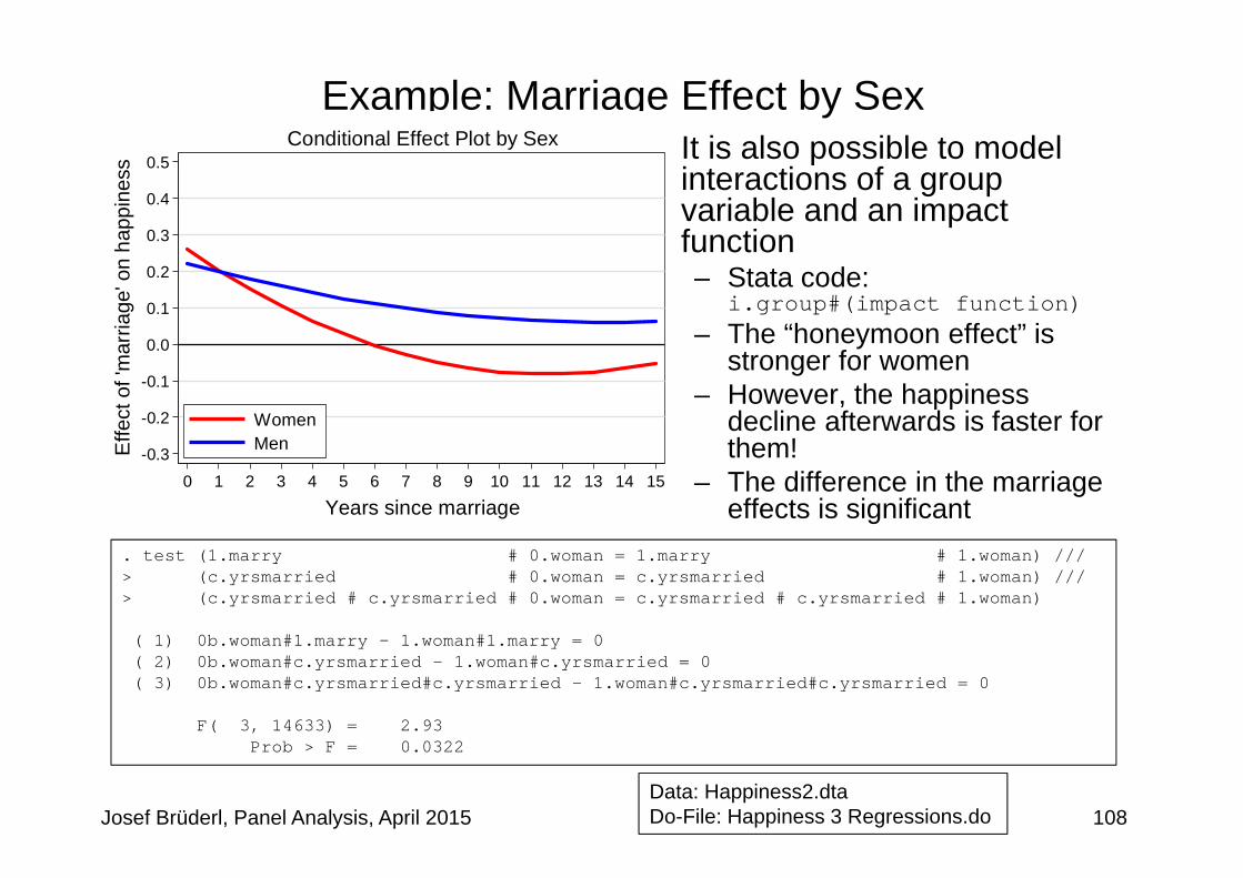
Example: Marriage Effect by Sex
108Data: Happiness2.dtaDo-File: Happiness 3 Regressions.do
• It is also possible to model interactions of a group variable and an impact function– Stata code:
i.group#(impact function)– The “honeymoon effect” is
stronger for women– However, the happiness
decline afterwards is faster for them!
– The difference in the marriage effects is significant
. test (1.marry # 0.woman = 1.marry # 1.woman) ///> (c.yrsmarried # 0.woman = c.yrsmarried # 1.woman) ///> (c.yrsmarried # c.yrsmarried # 0.woman = c.yrsmarried # c.yrsmarried # 1.woman)
( 1) 0b.woman#1.marry - 1.woman#1.marry = 0( 2) 0b.woman#c.yrsmarried - 1.woman#c.yrsmarried = 0( 3) 0b.woman#c.yrsmarried#c.yrsmarried - 1.woman#c.yrsmarried#c.yrsmarried = 0
F( 3, 14633) = 2.93Prob > F = 0.0322
-0.3
-0.2
-0.1
0.0
0.1
0.2
0.3
0.4
0.5
Effe
ct o
f 'm
arria
ge' o
n ha
ppin
ess
0 1 2 3 4 5 6 7 8 9 10 11 12 13 14 15
Years since marriage
WomenMen
Conditional Effect Plot by Sex

Interaction of Two Time-Varying Variables• In the same way we can specify the interaction of two time-
varying variables– Now the interaction can be interpreted symmetrically, because both
main effects are in the model– Thus, we have to decide which variable is the “treatment”, and
which one is the “moderator”- Interpretation: The “treatment effect” varies by level of “moderator”
• Example: How varies the marriage effect by HHincome?– HHincome measured in absolute terms ( in 10,000 EUR and top
coded at 50,000 EUR)
Josef Brüderl, Panel Analysis, April 2015 109
. xtreg happy i.marry##c.hhinct age, fe vce(cluster id)
--------------------------------------------------------------------------------| Robust
happy | Coef. Std. Err. t P>|t| [95% Conf. Interval]---------------+----------------------------------------------------------------
1.marry | .0522104 .0470784 1.11 0.267 -.0400692 .14449hhinct | .0556164 .0068092 8.17 0.000 .0422696 .0689632
marry#c.hhinct | .037676 .0136458 2.76 0.006 .0109286 .0644234

-0.10
-0.05
0.00
0.05
0.10
0.15
0.20
0.25
0.30
0.35
0.40
Effe
ct o
f 'm
arria
ge' o
n ha
ppin
ess
0 1 2 3 4 5HHincome (in 10,000 EUR)
Conditional Effect Plot by HHincome
Example: Marriage Effect by HHincome
Josef Brüderl, Panel Analysis, April 2015 110
Data: Happiness2.dtaDo-File: Happiness 3 Regressions.do
Effects of Consecutive Life Course Events• Until now we always investigated only one specific transition• Often researchers analyze several transitions in one analysis
(single estimation sample strategy)– Effects of different relationship types on happiness/wages– Effects of different parity births on wage (motherhood wage penalty)
• When interpreting results from such a single estimation sample strategy one has to be careful– Within estimation compares the outcome in the reference state with
the outcome in the focus state - Only for those, who were observed in both states- I.e., the reference group differs for each state
– This makes it problematic to compare the effects of different states
• Therefore, it is recommended to construct special estimation samples for every single transition of interest– Multiple estimation samples strategy
Josef Brüderl, Panel Analysis, April 2015 111

Example: Effect of Relationship Type on Wage• Categorical treatment variable: three relationship types
– Single, LAT, cohabitation (ref.: single)- Those starting a relationship first enter a LAT, eventually later a cohab
– Single estimation sample strategy- LAT-effect: wage difference single-LAT
- For all those, who enter a relationship- Cohab-effect: wage difference single-cohab
- Only for those, who eventually enter a cohab– Problem 1: The cohab-effect is not a causal effect, because there
is no observed transition from single to cohab– Problem 2: We cannot interpret LAT-effect minus cohab-effect!
- Because these effect estimates are based on different populations.- If the two populations have different LAT-effects (effect heterogeneity)
the LAT-cohab difference will be biased
• Multiple estimation samples strategy– The LAT-effect is estimated with all single/LAT person-years– The cohab-effect is estimated with all LAT/cohab person-years
Josef Brüderl, Panel Analysis, April 2015 112

0
1000
2000
3000
4000
5000
EU
RO
per
mon
th
1 2 3 4 5 6Time
single LAT Cohabitation
No Effect Heterogeneity – No Problem• (1) uses all pyrs
– Without effect heterogeneity we can interpret the difference in model (1)
– The causal effect of changing from LAT to cohabitation is zero
• (2) uses only pyrs in single or LAT
– The result is identical to (1)• (3) uses only pyrs in LAT or
cohabitation– The result shows that we can
interpret the difference in (1)
Josef Brüderl, Panel Analysis, April 2015 113
-----------------------------------------------------FE regress | (1)all pyrs (2)single/LAT (3)LAT/cohab-------------+---------------------------------------single | (ref.) (ref.)LAT | 500*** 500*** (ref.) cohabitation | 500*** 0 -------------+---------------------------------------
pers-yrs | 20 16 12 persons | 4 4 4
-----------------------------------------------------
Model (1): 500(3): 0
Data: Cat Treatment.dtaDo-File: Cat Treatment.do

0
1000
2000
3000
4000
5000
EU
RO
per
mon
th
1 2 3 4 5 6Time
single LAT Cohabitation
Effect Heterogeneity - Problem• (1) uses all pyrs
– It seems, as if the effect of a change from LAT to cohabitation is +125 €
– However, because the low LAT-effect people do not enter in a cohabitation, this is biased
• (3) uses the proper estimation sample– We see that the effect of a
change from LAT to cohabitation is in fact zero!
Josef Brüderl, Panel Analysis, April 2015 114
-----------------------------------------------------FE regress | (1)all pyrs (2)single/LAT (3)LAT/cohab-------------+---------------------------------------single | (ref.) (ref.)LAT | 250** 250** (ref.) cohabitation | 375** 0 -------------+---------------------------------------
pers-yrs | 20 16 12 persons | 4 4 4
-----------------------------------------------------
Model (1): 375(3): 0
Data: Cat Treatment.dtaDo-File: Cat Treatment.do

Another Example: Motherhood Status Penalty• The same problem occurs with research on cumulative
(dis)advantage– Abendroth et al. (2014) estimate effects of first, second, and third
births on women's status trajectories- Data: ECHP 1994 to 2001, 13,615 women aged 18 to 40 in 13 countries- Outcome: ISEI status score- Treatment: parity specific birth dummy and linear event time variable- Status trajectory is modeled with linear and quadratic age terms- Estimation sample:
All women entering the labormarket 1994 – 2001 (some had already children)
- Estimation strategy:they use all pyrs and estimatea FE regression with allparities in one model(single estimation sample)
Josef Brüderl, Panel Analysis, April 2015 115
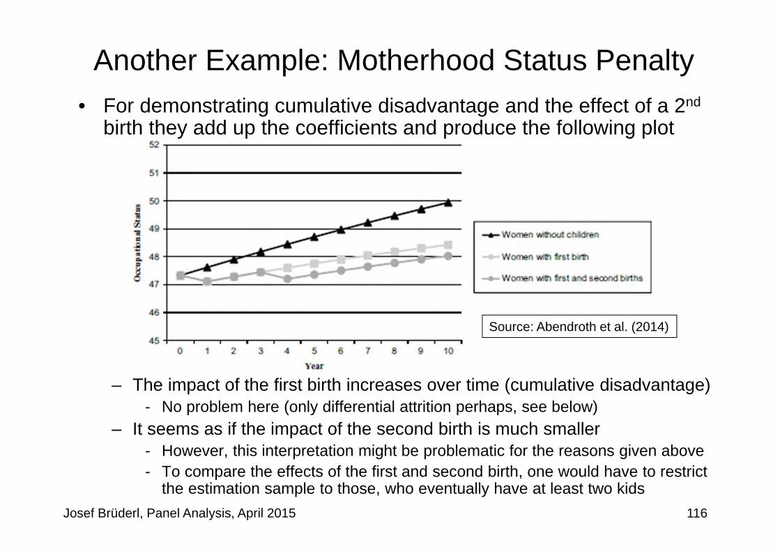
• For demonstrating cumulative disadvantage and the effect of a 2nd
birth they add up the coefficients and produce the following plot
– The impact of the first birth increases over time (cumulative disadvantage)- No problem here (only differential attrition perhaps, see below)
– It seems as if the impact of the second birth is much smaller- However, this interpretation might be problematic for the reasons given above- To compare the effects of the first and second birth, one would have to restrict
the estimation sample to those, who eventually have at least two kids
Another Example: Motherhood Status Penalty
Josef Brüderl, Panel Analysis, April 2015 116
Source: Abendroth et al. (2014)
Chapter VI: Modeling Individual Growth
Josef BrüderlApplied Panel Data Analysis
Section: Growth Curve Models

Josef Brüderl, Panel Analysis, April 2015
Modeling Individual Growth• How develops an outcome over age?
– (Multi-cohort) panel data allow to separate age and cohort effects!– Thereby we can model individual growth
- This is the second major advantage of panel data
• Growth curve (GC)– Development of the outcome over age (A) net of cohort (C)
– This is a linear growth curve, but it is easy to model quadratic, cubic, etc. growth curves
- Most flexible: age (group) dummies, splines (cf. Wunder et al. 2013)– Can age have a “causal” effect?
- In a narrow sense of causality, age can not be seen as a cause, because it is not manipulable
- However, in a mechanism based approach age is seen as a correlate of intervening mechanisms that potentially can be manipulated
118

Josef Brüderl, Panel Analysis, April 2015
Cross-Sectional Data• Thought experiment: estimating a growth curve from cross-sectional data
– We assume that happiness declines linearly with age (age effect)– We assume that younger cohorts are happier (cohort effect)– There is no period effect
• Cross-sectional survey in the year 2000– The estimated growth curve is red dashed: It mixes age and cohort effect– It is impossible to separate age and cohort effect!
age
happiness
20 30 40 50 60
1950
1960
1970
119

Josef Brüderl, Panel Analysis, April 2015
Panel Data• Thought experiment: estimating a growth curve from panel data
– We assume that happiness declines linearly with age (age effect)– We assume that younger cohorts are happier (cohort effect)– There is no period effect
• Panel survey in the years 1990, 2000, and 2010– The estimated growth curves (not shown) are identical with the true ones– It is possible to separate age and cohort effect!
age
happiness
20 30 40 50 60
1950
1960
1970
120
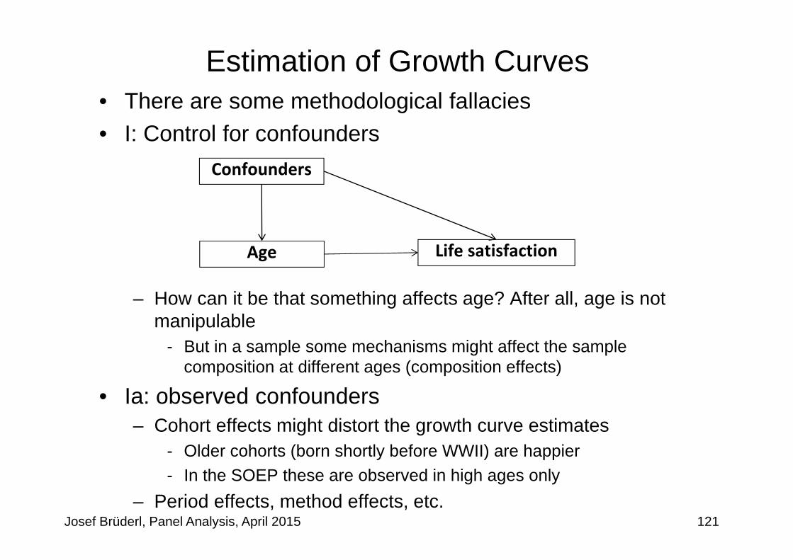
Estimation of Growth Curves• There are some methodological fallacies• I: Control for confounders
– How can it be that something affects age? After all, age is not manipulable
- But in a sample some mechanisms might affect the sample composition at different ages (composition effects)
• Ia: observed confounders– Cohort effects might distort the growth curve estimates
- Older cohorts (born shortly before WWII) are happier- In the SOEP these are observed in high ages only
– Period effects, method effects, etc.Josef Brüderl, Panel Analysis, April 2015 121
Age Life satisfaction
Confounders

Estimation of Growth Curves• Ib: Unobserved confounders (self selection)
– Selection might distort the growth curve estimates- Due to differential mortality (e.g., happier people survive longer)- Due to differential attrition (e.g., happier people attrite less)
– Selectivity might bias estimates of covariate effects and that might indirectly bias the age effect (Frijters/Beatton 2012)
• Methodological lesson I– Control at least for observables– Even better: estimate FE growth curves
- FE analysis provides a within estimate of the age effect- How does happiness change, if a respondent grows one year older?- Therefore, sample composition/selection does not bias the age effect
- There is a better chance to have unbiased covariate effects– This point has been overseen in most of the literature that estimates
GCs by RE (or POLS) methods- Many of the GCs reported in the literature will be biased
Josef Brüderl, Panel Analysis, April 2015 122

Estimation of Growth Curves• II: Overcontrol might distort the growth curve estimates
– Generally: When estimating causal effects, one should control confounders, but not intervening mechanisms
– Otherwise you will get “overcontrol bias”- Overcontrol is the consequence of a “kitchen sink approach” that
unfortunately is very common in social research based on regressions
• Methodological lesson II– Do not control for intervening mechanisms– First, get the gross causal effect of age by controlling for
confounders only– In a second step, try to get closer on the intervening mechanisms
by adding them to the modelJosef Brüderl, Panel Analysis, April 2015 123
Age Life satisfaction
Health
Family events
Biol. ageing
Human capital
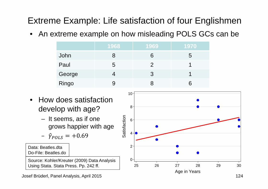
0
2
4
6
8
10
Sat
isfa
ctio
n
25 26 27 28 29 30Age in Years
Extreme Example: Life satisfaction of four Englishmen• An extreme example on how misleading POLS GCs can be
• How does satisfaction develop with age?– It seems, as if one
grows happier with age– 0.69
124
1968 1969 1970John 8 6 5Paul 5 2 1George 4 3 1Ringo 9 8 6
Source: Kohler/Kreuter (2009) Data Analysis Using Stata. Stata Press. Pp. 242 ff.
Data: Beatles.dtaDo-File: Beatles.do
Josef Brüderl, Panel Analysis, April 2015

0
2
4
6
8
10
Sat
isfa
ctio
n
25 26 27 28 29 30Age in Years
• However, between estimation is completely misleading here– Because there is heterogeneity between the men (perhaps a cohort effect?)
• Within estimation shows that there is actually a negative age effect!– Estimate separate regression lines for each man: All men grow less happy
- Green ( 2.0), orange, blue, brown ( 1.5)- The FE estimate is the average of these four slopes
. . . . 1.625
125
Data: Beatles.dtaDo-File: Beatles.do
Josef Brüderl, Panel Analysis, April 2015
Extreme Example: Life satisfaction of four Englishmen

. xtreg happy c.age##c.age##c.age , fe vce(cluster id)
-------------------------------------------------------------------------------| Robust
happy | Coef. Std. Err. t P>|t| [95% Conf. Interval]------------------+------------------------------------------------------------
age | -0.1343 0.0128 -10.50 0.000 -0.1594 -0.1092c.age#c.age | 0.0025 0.0003 7.71 0.000 0.0019 0.0032
c.age#c.age#c.age | -0.0000 0.0000 -7.95 0.000 -0.0000 -0.0000------------------+------------------------------------------------------------
. margins, at(age=(18(4)98))
. marginsplot, recast(line) recastci(rline)
Happiness Example: Specification of Growth Curves
• After explorative analyses we decided to use a cubic specification– Wunder et al. (2013) argue that a cubic polynomial does not adequately
represent happiness growth. They suggest semi-parametric splines. Below we will use the most flexible age dummy specification.
• Cohort is controlled by introducing 90 birth year dummies– With i.cohort (not in the FE model!)
• GC estimation results can best be visualized by a profile plot– Please note that the FE profile plot rests on adding an arbitrary constant!
Josef Brüderl, Panel Analysis, April 2015 126
Data: Happiness2.dtaDo-File: Happiness 4 Regressions.do

0123456789
10H
appi
ness
10 20 30 40 50 60 70 80 90 100
Age
a) POLS without controlling for cohort
0123456789
10
Hap
pine
ss
10 20 30 40 50 60 70 80 90 100
Age
b) POLS with controlling for cohort
0123456789
10
Hap
pine
ss
10 20 30 40 50 60 70 80 90 100
Age
c) RE with controlling for cohort
0123456789
10
Hap
pine
ss
10 20 30 40 50 60 70 80 90 100
Age
d) FE (implicitly controlling for cohort)
Happiness Example: Comparing Different Specifications
Josef Brüderl, Panel Analysis, April 2015 127
Data: Happiness2.dtaDo-File: Happiness 4 Regressions.do

Happiness Example: Comparing Different Specifications
• See previous slide– Panel a): POLS without controlling for cohort
- This is a grossly mis-specified model! We find a U-shaped GC. However, this is an artifact, since older cohorts are happier.
- Nevertheless, many studies in the economics literature report such an U-shape and take it seriously! (Wunder et al. 2013)
– Panel b): POLS with controlling for cohort- Now we see declining happiness- Nevertheless, this is still biased upwards, because happier people live
longer (self-selection into higher ages)– Panel c): RE with controlling for cohort
- The late age decline becomes steeper- Nevertheless still a small upward bias
– Panel d): FE (implicitly controlling for cohort)- Within estimation shows that the late age decline is even more sharp- Before age 60 happiness declines slowly.
Josef Brüderl, Panel Analysis, April 2015 128

Chapter VI: Modeling Individual Growth
Josef BrüderlApplied Panel Data Analysis
Section: The Age-Period-Cohort Problem
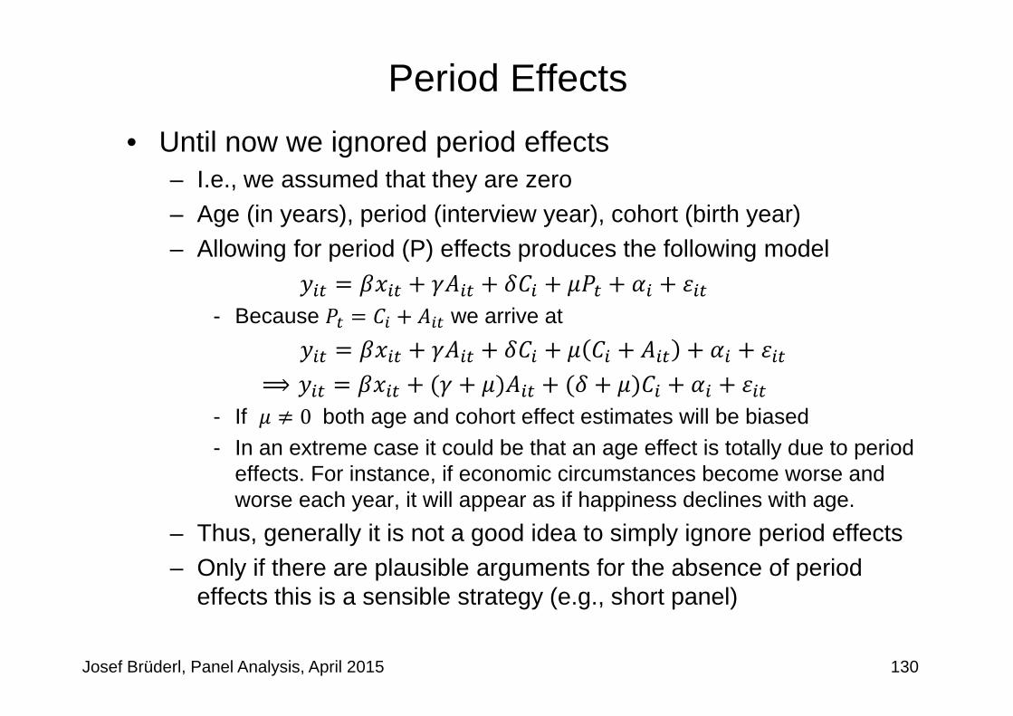
Josef Brüderl, Panel Analysis, April 2015
Period Effects• Until now we ignored period effects
– I.e., we assumed that they are zero– Age (in years), period (interview year), cohort (birth year)– Allowing for period (P) effects produces the following model
- Because we arrive at
⟹- If 0 both age and cohort effect estimates will be biased- In an extreme case it could be that an age effect is totally due to period
effects. For instance, if economic circumstances become worse and worse each year, it will appear as if happiness declines with age.
– Thus, generally it is not a good idea to simply ignore period effects– Only if there are plausible arguments for the absence of period
effects this is a sensible strategy (e.g., short panel)
130

Josef Brüderl, Panel Analysis, April 2015
Period Effect Biasing the Age Effect
age
happiness
20 30 40 50 60
1950
1960
1970
131
• Thought experiment: estimating a growth curve from panel data– We assume that happiness declines linearly with age (age effect)– We assume that younger cohorts are happier (cohort effect)– We assume that winning the world championship 1990 made people
temporarily happier (period effect)
• Panel survey in the years 1990, 2000, and 2010– The estimated growth
curves are too steep- Ignoring the period effect
biases the age effect– Adding a 1990-dummy
would produce unbiased results, because the period effects are then correctly specified

Josef Brüderl, Panel Analysis, April 2015
The Age-Period-Cohort (APC) Problem• The fundamental identification problem
– This is the model with all three terms
- We have linear dependence because - Due to collinearity it is impossible to estimate all three effects- The model is not identified- It does not matter, whether the terms enter linearly or as dummies
– Variant: two-way FE model
- Here only age and period terms are specified. However, is person-specific and therefore included in the fixed-effects
- The period term is here specified as year (wave) dummies . One year dummy has to be dropped (base category)
- This model is not identified. With FE estimation already an age-period specification is not identified
– The same problem one has with a single cohort panel- An age-period specification (POLS) is not identified
132

Josef Brüderl, Panel Analysis, April 2015
The APC Problem: Solutions• One has to impose (sensible) APC restrictions
– Equality constraints- Example period dummies: at least a second period dummy has to be
dropped. But which one?- Stata default: the last period dummy is dropped additionally- Hand made: use a RE-model (with cohort restriction) and look for years
with similar outcome values, and use these as base- Problem: RE estimated with cohort restriction!
– The age effect could be specified non-linear- For instance, include only a quadratic age term- This method often produces nonsense
– Specify at least one term as a step function- At least one term has to be grouped
- Often 5-year cohorts (or “war cohort”, “baby boomers”, etc.)- Terms could be grouped with different interval length
- For instance, 5-year periods and 10-year age groups
133

Josef Brüderl, Panel Analysis, April 2015
Happiness Example: The Stata Default Solution
. xtreg happy c.age##c.age##c.age i.year, fe vce(cluster id)
note: 2009.year omitted because of collinearity
-----------------------------------------------------------------------------------| Robust
happy | Coef. Std. Err. t P>|t| [95% Conf. Interval]------------------+----------------------------------------------------------------
age | -0.1373 0.0129 -10.64 0.000 -0.1626 -0.1120c.age#c.age | 0.0026 0.0003 7.76 0.000 0.0019 0.0032
c.age#c.age#c.age | -0.0000 0.0000 -8.01 0.000 -0.0000 -0.0000|
year |1984 | 0.0000 (base)1985 | -0.0478 0.0454 -1.05 0.292 -0.1367 0.04111986 | 0.0502 0.0452 1.11 0.267 -0.0384 0.1388
...2007 | 0.0733 0.0207 3.54 0.000 0.0327 0.11382008 | 0.0690 0.0199 3.47 0.001 0.0301 0.10802009 | 0.0000 (omitted)
------------------+----------------------------------------------------------------
Letting Stata decide which restriction to use:
134
Data: Happiness2.dtaDo-File: Happiness 4 Regressions.do

Happiness Example: APC Restrictions• Unfortunately, the estimated age effect is often very
sensitive to the restrictions chosen• On the next slide we demonstrate, how different APC
restrictions affect a cubic RE happiness GC– We use RE, because then we have full flexibility in specifying the
restrictions (e.g., we can drop “cohort” from the model)– Panel a): age-cohort model (period dummies missing)
- Mis-specified because there are period effects– Panel b): age-period model (cohort dummies missing)
- Mis-specified because there are cohort effects– Panel c): age-period-cohort model (cohort grouped)– Panel d): age-period-cohort model (some period dummies miss.)
- Our favorite model: 1984/85/86/90/91 are the base. A RE model (without cohort) showed that these years have the highest and very similar happiness levels
- Here we see that the growth curve is essentially flat until 70Josef Brüderl, Panel Analysis, April 2015 135

0123456789
10H
appi
ness
10 20 30 40 50 60 70 80 90 100
Age
a) period (missing), cohort (dummies)
0123456789
10
Hap
pine
ss
10 20 30 40 50 60 70 80 90 100
Age
b) period (dummies), cohort (missing)
0123456789
10
Hap
pine
ss
10 20 30 40 50 60 70 80 90 100
Age
c) period (dummies), cohort (10 yrs groups)
0123456789
10
Hap
pine
ss
10 20 30 40 50 60 70 80 90 100
Age
d) period (84/85/86/90/91 base), cohort (dummies)
Happiness Example: Comparing Different APC Restrictions
Josef Brüderl, Panel Analysis, April 2015 136

The APC Problem: A Better Solution• Obviously, APC restrictions are problematic• “Substantive” solution for the APC problem
– For similar arguments see Wunder et al. (2013)– Do not use the proxy variable “period”, but specify the events that
produced the period effects directly- Under good economic circumstances (GDP) happiness should be higher- Fall of the wall and German unification: happiness increase 1990/91- Germany became soccer world champion: increase in 1991- Panel conditioning: happiness is higher in the first waves
– Alternatively the same could be done with the cohort effect- People who lived during a war might be happier afterwards
• Recommendation– Age and cohort effects are in most applications most “important”
- Include those in all panel regressions (age and cohort dummies)– Then start thinking about potential period effects
- Include only the relevant “period variables”Josef Brüderl, Panel Analysis, April 2015 137

0
1
2
3
4
5
6
7
8
9
10
Hap
pine
ss
10 20 30 40 50 60 70 80 90 100
Age
Our Final Result on Happiness Growth• Using all SOEP pyrs 18-90 (v29, 1984-2012); N·T=470,022, N=57,758• FE model (controls implicitly for all time-constant confounders)
– Fully flexible specification through age dummies– Period variables: unemployment rate, GDP growth rate– Panel conditioning: wave 1-3 dummies
Josef Brüderl, Panel Analysis, April 2015 138
– Happiness decline up to age 60
– There is a little “pension hump” after age 60 (Wunder et al. 2013)
– Happiness declines sharply after age 65- Terminal decline 3-5
years before death: “Death is lurking around the corner” (Gerstorf et al. 2010)
Source: Kratz/Brüderl (2015)

Chapter VI: Modeling Individual Growth
Josef BrüderlApplied Panel Data Analysis
Section: Group Specific Growth Curves

Group Specific Growth Curves (GCs)• Interact age with a time-constant group variable ( : 0,1 )
– Here the question is not on group-specific age effects (see Chap.V)– But on the group difference in the outcome and
how it develops over age- Therefore, we need models with a group main effect- It makes sense to center age
• Example: linear GC [(uncentered) age is ]
the group difference at 0the change in the group difference with every year
- Stata code: i.group##c.age
• Group specific growth curves provide much more information on the effect of a time-constant variable than a simple group effect– It is a waste of panel data to estimate only group effects!!! – Instead estimate group specific growth curves!
Josef Brüderl, Panel Analysis, April 2015 140

0
1
2
3
4
5
6
7
8
9
10
Hap
pine
ss
0 10 20 30 40 50 60 70 80 90 100
Age
WomenMen
0
1
2
3
4
5
6
7
8
9
10
Hap
pine
ss
0 10 20 30 40 50 60 70 80 90 100
Age
WomenMen
Happiness Example: FE Estimation
With FE we obtain a strange result– It seems, as if women are much
more happy (more than one scale point!) (upper Fig.)
– However, this is nonsense: In FE there is no main effect of “sex” - Therefore, FE forces the restriction of
equal happiness at age 0.- Therefore, the difference between the
GCs is not interpretable- If we center “age” (mean=29.3), a
different restriction applies and now men seem to be happier (lower Fig.)
– Thus, group-specific GCs can not be estimated with FE!
– Unfortunately there is no way around this problem- Separate FE regressions for men and
women also provide no well defined constant
- A Hybrid model (see below) has a main sex effect, but this is a between constant. Within results are identical with FE.
Josef Brüderl, Panel Analysis, April 2015 141
Data: Happiness2.dtaDo-File: Happiness 4 Regressions.do

Happiness Example: RE Estimation• Therefore, in the following we estimate RE-GCs.
– Fortunately with long panels RE-GCs are generally close to FE-GCs- This can be checked by comparing the FE-GC and the RE-GC
– Note, the group effect might be affected by unobserved heterogeneity- Again this reflects the fact, that there is no within variation to estimate the
group effect. We have to use the between variation. Nevertheless, RE-GCs make much better use of the between variation in panel data
• The results (see next slides)– Age should be centered (agec)
- Thus the sex main effect is the happiness difference at age 29.3– Profile plot: women are happier around age 30 and at higher ages
- To asses the significance of the sex differences one has to use a conditional effect plot
– Conditional effect plot: women are significantly happier than men from about age 25 to age 40! Difference is +0.09 points at about age 35.
- Obviously, this is much more information than what a simple sex effect (+0.03) from a RE model tells us!
Josef Brüderl, Panel Analysis, April 2015 142

Happiness Example: Sex Specific RE-GCs
Josef Brüderl, Panel Analysis, April 2015 143
. xtreg happy marry loghhinc i.woman i.woman#(c.agec##c.agec##c.agec) /// > ib(last).cohort i(1987/1989 1992/2009)bn.year, re vce(cluster id)
Random-effects GLS regression Number of obs = 121919Group variable: id Number of groups = 14634
R-sq: within = 0.0199(Std. Err. adjusted for 14634 clusters in id)
--------------------------------------------------------------------------------------------| Robust
happy | Coef. Std. Err. z P>|z| [95% Conf. Interval]---------------------------+----------------------------------------------------------------
marry | .1902277 .0202162 9.41 0.000 .1506048 .2298507loghhinc | .1890756 .0110697 17.08 0.000 .1673793 .2107719
1.woman | .0812636 .0280571 2.90 0.004 .0262727 .1362545|
woman#c.agec |0 | -.0143229 .0062536 -2.29 0.022 -.0265797 -.00206611 | -.010067 .0062785 -1.60 0.109 -.0223725 .0022386
|woman#c.agec#c.agec |
0 | .0008397 .0001548 5.43 0.000 .0005363 .0011431 | .0003486 .0001542 2.26 0.024 .0000462 .0006509
|woman#c.agec#c.agec#c.agec |
0 | -.0000192 4.16e-06 -4.61 0.000 -.0000273 -.0000111 | -.0000114 2.89e-06 -3.94 0.000 -.000017 -5.71e-06
Age-cohort-period(84/85/86/90/91 base) specification

0
1
2
3
4
5
6
7
8H
appi
ness
20 30 40 50 60 70 80 90
Age
WomenMen
profile plot
-1.00
-0.75
-0.50
-0.25
0.00
0.25
0.50
0.75
1.00
1.25
1.50
AM
E o
f 'w
oman
' on
happ
ines
s20 30 40 50 60 70 80 90
Age
conditional effect plot
Josef Brüderl, Panel Analysis, April 2015 144
Data: Happiness2.dtaDo-File: Happiness 4 Regressions.do
margins woman, at(agec=(-10(5)60))marginsplot, recast(line) noci
margins , at(agec=(-10(5)60)) dydx(woman)marginsplot, recast(line) recastci(rline)
Happiness Example: Sex Specific RE-GCs

Example: The Cost of Breastfeeding• Group specific GCs are mostly used in a purely descriptive manner.
However, in a complex social world this type of description is very informative• Example: Mothers‘ income trajectories after the birth of the first child
– Cubic growth curves: time since childbirth (year prior birth=0)– By infant feeding type
Josef Brüderl, Panel Analysis, April 2015 145
Source: Rippeyoung/Noonan (2012)

Example: Body Weight Growth
Josef Brüderl, Panel Analysis, April 2015 146
• Pairfam (v5) data on body weight– Pairfam has three cohorts that do not yet overlap– Note the smooth trajectories (data seem to be valid!)– There is a clear cohort effect visible: The younger cohorts are on an
ever higher trajectory (secular increase in height [and thereby weight])
Source: Bernadette Huyer-May, unpublished work

Chapter VII: Further Linear Panel Models
Josef BrüderlApplied Panel Data Analysis
Section: Alternative Within Estimators

LSDV: areg• areg is a LSDV estimator
– Person dummies are not estimated, but absorbed– is variance explained including the person dummies
- I.e., it is very large (it is not the within )– areg S.E.s are larger than xtreg S.E.s
- areg assumes that the number of persons does not increase with sample size (only then the estimates of person dummies are consistent)
- xtreg does not rest on this assumption– areg allows for panel weights that change over waves
- xtreg does not!
• Recommendation– Use areg only, if you want to do weighted FE estimation– This is detailed below
Josef Brüderl, Panel Analysis, April 2015 148

Individual Slope Regression• The FE estimator is the weighted average of the slopes of
the individual regressions– Weighted by the length of the individual panels– Only true for the bivariate model
Josef Brüderl, Panel Analysis, April 2015 149
. keep if pycount == 26 //only panels with 26 observations (equal weight!)
. xtreg happy age, fe //benchmark FE model------------------------------------------------------------------------------
happy | Coef. Std. Err. t P>|t| [95% Conf. Interval]-------------+----------------------------------------------------------------
age | -.0236349 .0017556 -13.46 0.000 -.0270764 -.0201935_cons | 8.078896 .0659529 122.49 0.000 7.949613 8.208179
------------------------------------------------------------------------------
. * Now we run 348 regressions!
. statsby cons=_b[_cons] slope=_b[age], by(id): regr happy age
. summ slope cons //perfectly identical
Variable | Obs Mean Std. Dev. Min Max-------------+--------------------------------------------------------
slope | 348 -.0236349 .0647752 -.2413675 .1480342cons | 348 8.099078 2.612797 -.3589744 21.8841
Data: Happiness2.dtaDo-File: Happiness 5 Regressions.do
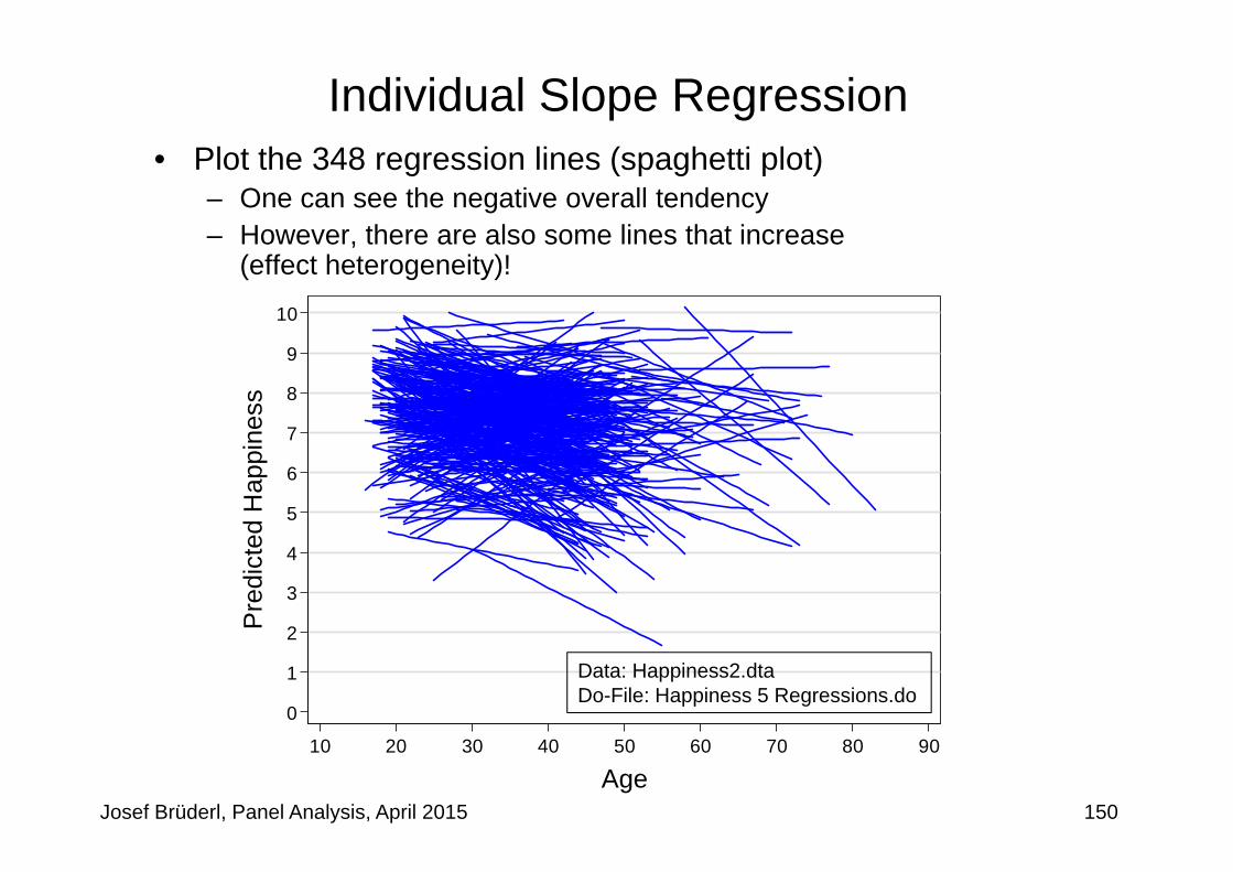
0
1
2
3
4
5
6
7
8
9
10
Pre
dict
ed H
appi
ness
10 20 30 40 50 60 70 80 90
Age
• Plot the 348 regression lines (spaghetti plot)– One can see the negative overall tendency– However, there are also some lines that increase
(effect heterogeneity)!
Josef Brüderl, Panel Analysis, April 2015 150
Individual Slope Regression
Data: Happiness2.dtaDo-File: Happiness 5 Regressions.do

Difference-in-Differences (DiD)• DiD can be implemented in a regression framework
- Post-treatment period dummy: - Treatment dummy: ‐ : pre-treatment mean outcome in control group‐ : post-treatment change in mean outcome in control group‐ : pre-treatment difference in mean outcome in treatment group‐ : post-treatment difference in change in mean outcome in treatment
group (this is the treatment effect)– DiD models only group differences. Therefore, it can be applied to
aggregate pseudo-panel data (trend data on the group level).– This makes DiD a very useful tool for policy analysis with data from
natural experiments (treatment and control groups are assigned without randomization)
– However, with individual panel data DiD makes less sense- Controls enter as levels (not differences) and therefore their effects will
be biased and this in turn can bias the treatment effect estimateJosef Brüderl, Panel Analysis, April 2015 151

Difference-in-Differences (DiD)
• With controls this is generally no longer true• Further, with non-policy (“natural”) treatments DiD is not
straightforward, because treatment does not occur at a fixed time point. – Then one lacks a clear before-after for the control group. One has
to use some kind of matching to construct the control group (DiD-matching).
Josef Brüderl, Panel Analysis, April 2015 152
• Without controls DiD is equivalent to FE. gen treat = id >= 3. gen post = time >= 4. gen posttreat = post * treat. regr wage post treat posttreat------------------------------------------------------------------------------
wage | Coef. Std. Err. t P>|t| [95% Conf. Interval]-------------+----------------------------------------------------------------
post | 2.32e-13 318.4598 0.00 1.000 -664.2956 664.2956treat | 2000 318.4598 6.28 0.000 1335.704 2664.296
posttreat | 500 450.3702 1.11 0.280 -439.4558 1439.456_cons | 1500 225.1851 6.66 0.000 1030.272 1969.728
------------------------------------------------------------------------------
Data: Wage Premium.dtaDo-File: Wage Premium.do

DiD-Matching Example: Poverty Risks • Kohler et al. (2012) investigate how welfare states protect
people from poverty after critical life events– Germany (conservative welfare state), U.S. (liberal welfare state)– Outcome: % in poverty (below 60% median equivalence income)– Treatment: job loss, sickness, retirement, family dissolution– Method: DiD (3 years before, 4 years after)
- Treatment group: 3 years not poor, then having a critical life event- Control group: exact matching (all those, who were also not poor in
these 3 years, and who did not have the event in the next four years)– Data: SOEP and PSID, 1984 - 2009– Results: see next slide– Criticism:
- Groups are selected according to the outcome (3 years not poor). Thus, in fact this is not DiD, it is only the post-treatment difference
- The construction of the control group is sub-optimal: exact matching without any controls. Better would be Propensity-Score DiD-matching.
Josef Brüderl, Panel Analysis, April 2015 153

DiD-Matching Example: Poverty Risks
Josef Brüderl, Panel Analysis, April 2015 154Source: Kohler et al. 2012

Chapter VII: Further Linear Panel Models
Section: The Fixed-EffectsIndividual-Slopes Model
Josef BrüderlApplied Panel Data Analysis

The Parallel Trends Assumption• Another way to express the strict exogeneity assumption
from a counterfactual perspective– Strict exogeneity implies, that the (potential) outcome trends in
treatment and control group must be parallel– Then the FE-estimate is consistent, and captures the treatment effect
Josef Brüderl, Panel Analysis, April 2015 156
EXP
ln W
Selection on level
Treatment effect
D
Observed outcomes
Potential outcomes
FE estimate

The Parallel Trends Assumption• Parallel trends assumption violated: heterogeneous growth
– Those on a steeper trajectory are selected into the treatment- E.g., younger cohorts might accumulate skills faster and self-select into treatment- E.g., career orientation may differ between those in treatment and control
– This is a violation of strict exogeneity due to time-varying unobservables– The FE-estimate will be biased upwards (in case of diverging trends)
- It includes the wage increase due to the steeper trend (“selection on growth”)
Josef Brüderl, Panel Analysis, April 2015 157
EXP
ln W
Selection on level
Selection on growth
Treatment effect
D
Observed outcomes
Potential outcomes
FE estimate

The FEIS Model• Due to group specific trends we have non-parallel trends• This can be generalized to individual specific trends
– This is the fixed-effects model with individual-specific constants and slopes (FEIS) (Wooldridge, 2010: pp. 377-381)
– captures individual differences in the growth of the outcome over time. is time-varying unobserved heterogeneity (heterogeneous growth).
– In a standard FE this is part of the idiosyncratic error term
– As shown below, we can get rid of – Thus, FEIS needs a weaker exogeneity assumption
- FE: , forall , 1, … ,- FEIS: , forall , 1, … ,
– In the FEIS model time-varying unobserved heterogeneity that is due to individual-specific trends is no longer a problem
Josef Brüderl, Panel Analysis, April 2015 158

How Can We Get Rid of the Individual-Specific Trends?• Including individual level and trend dummies (LSDV)
– This is done often intuitively in studies with country data: POLS models include country-specific intercepts and country-specific trends
• Second-differences estimator (SD)
12
– Computing first differences (FD)
– Now take second differences (SD)2 2 2
– With this extension of FD we managed to get rid of and . Using POLS provides an unbiased estimate of , if the exogeneity assumption on holds.
– SD needs at least 3 waves– SD is efficient with 3. It is inefficient for 3
Josef Brüderl, Panel Analysis, April 2015 159

FEIS Estimation• Detrending transformation (FEIS estimation)
– Analogous to FE, where data are demeaned, we “detrend” the data1) Estimate for each unit the individual growth curve
and get predicted values 2) Subtract predicted values from actual outcomes to get detrended
outcomes 3) Repeat steps 1) and 2) to detrend also the regressors 4) Pool the detrended data and run a POLS regression
– The intuition is that after detrending only variation around the trend is left. Only this around-trend variation is used to estimate the causal effect. Thus, heterogeneous growth can no longer bias estimates
• This approach can be generalized (see next slide)– Trends of higher order can be modeled– Individual slopes for non-time variables can be dealt with analogously– An ado xtfeis.ado is obtainable from Volker Ludwig
Josef Brüderl, Panel Analysis, April 2015 160

The General FEIS Model• The general model is
where is a 1 vector of variables with individual-specific slopes (including a constant)– For detrending one needs at least 1 observations– The detrended model is
– Note that after detrending also has gone. FEIS provides no effect estimates for the
– To get consistent estimates, it must hold, forall , 1, … ,
– which is a weaker form of the strict exogeneity assumption from FE estimation
- Idiosyncratic errors are expected to be unrelated to regressors only conditional on individual slopes
Josef Brüderl, Panel Analysis, April 2015 161

Example: Testing for Heterogeneous Growth
• An explorative test on the group level– Interact the linear age trend with an indicator for treatment (FE)
– We see that the treatment group shows a significantly less steeper happiness decline
– However, this might simply be due to the positive treatment effect (that in this specification is only controlled by the marriage dummy)
– Thus, we include distributed FEs up to 6
– Now there is no longer a significant non-parallel trendJosef Brüderl, Panel Analysis, April 2015 162
xtreg happy marry i.treat##c.age loghhinc, fe vce(cluster id)------------------------------------------------------------------------------
happy | Coef. Std. Err. t P>|t| [95% Conf. Interval]-------------+----------------------------------------------------------------
marry | .1321504 .0233535 5.66 0.000 .0863746 .1779262age | -.0446538 .0024492 -18.23 0.000 -.0494546 -.0398531
1.treat#c.age| .0076853 .0033946 2.26 0.024 .0010315 .0143391
xtreg happy i.ym i.treat##c.age loghhinc, fe vce(cluster id)------------------------------------------------------------------------------
happy | Coef. Std. Err. t P>|t| [95% Conf. Interval]-------------+----------------------------------------------------------------
..... |age | -.0446845 .002449 -18.25 0.000 -.0494849 -.0398842
1.treat#c.age| .0099943 .0088322 1.13 0.258 -.0073178 .0273065

Happiness Example: FEIS
• We allow for heterogeneous growth (FEIS1), heterogeneous income effects (FEIS2), or both (FEIS3)– Note that is smaller, because all models are estimated with 3 (FEIS3 4)– Given the explorative results from above it is not surprising that the marriage effect is
not much affected by allowing for heterogeneous growth– However, the income effect is strongly reduced by allowing for heterogeneous growth
- Those on a less declining happiness trajectory get more likely an income increase
Josef Brüderl, Panel Analysis, April 2015 163
xtfeis happy marry loghhinc, slope(age) cluster(id) //FEIS1--------------------------------------------------------------
Variable | FE FEIS1 FEIS2 FEIS3 -------------+------------------------------------------------
marry | 0.1675 0.1599 0.1616 0.1462 | 7.3696 6.3837 6.5204 5.3227
age | -0.0412 -0.0437 | -23.9129 -21.5316
loghhinc | 0.1255 0.0796 | 10.1681 5.9522
-------------+------------------------------------------------N | 118201 118201 118201 113266
--------------------------------------------------------------legend: b/tData: Happiness2.dta
Do-File: Happiness 5 Regressions.do

Ludwig, Volker and Josef Brüderl (2011) Is There a Male Marital Wage Premium? Resolving an Enduring Puzzle with Panel Data from Germany and the U.S. Unpublished manuscript.

The Male Marital Wage Premium (MWP)• Married men earn more than unmarried men
– “… one of the most well documented phenomena in social science” (Waite & Gallagher 2000: 99)
• Early studies used cross-sectional data– Self-selection: high wage men more attractive marriage partners
• However, also recent longitudinal studies find a MWP– Ahituv/Lerman (2007) Demography
NLSY79, FE (fixed-effects) regression: 7.6 %– Pollmann-Schult (2011) European Soc. Rev.
SOEP 1985-2008, FE regression: 4.2 %
• Thus, using the best available data and methodology, it seems marriage makes men more productive workers– Remark: Not the effect on labor hours is investigated here,
but the effect on productivity (gross hourly wage rate)
• However, we are not convinced– Self-selection may operate on wage growth (not only on level)
165Josef Brüderl, Panel Analysis, April 2015

Explanations for a Causal MWP
• Family economics (Becker 1981)– Precondition: there is a traditional division of labor
– Married men specialize on market work They accumulate more market specific skills
– Married women specialize on household work Married men are released from strenuous houseworkThey can put more effort in their market work
• Lifestyle explanation– After marriage men are domesticated by their wives
• Demand side explanation– Paternalism of employers
specialization
work effort
domestication
employer favoritism
166Josef Brüderl, Panel Analysis, April 2015

Arguments for a Spurious MWP
• (Self)-selection of high wage males into marriage– They gain more from specialization and therefore are more willing
to marry– They are more attractive marriage partners
- Due to their higher wage- Due to other unobservables correlated with wage
e.g. cognitive skills, social skills, beauty
• It is not only level, but also „steepness“ of the career– Promising young men (steep wage-profile) are attractive partners– Standard FE models yield upwardly biased estimates
• To get unbiased estimates one should use FEISln
where exp is labor market experience
167Josef Brüderl, Panel Analysis, April 2015

Data and Variables• SOEP v27, 1984-2010 and NLSY79, 1979-2004
• Outcome: deflated log. hourly wage– NLSY: reported hourly gross earnings
– SOEP: monthly gross earnings, divided by actual work hours * 4.36
• Treatment: marital status– Derived from (monthly) marriage biography, 4 states
- Never-married, 1st marriage, separated/divorced, remarriage
• Control variables– Labor market experience (linear and squared)
– Years of education
– Currently enrolled in education
– Firm tenure (yrs.)
– Number of (biological) children
– Dummies for survey year168Josef Brüderl, Panel Analysis, April 2015

Sample Restrictions• SOEP
– West German resident males
– Cohorts 1946 to 1975
– No self-employees, private sector workers
– Never-married when first observed, at least 4 obs. (N=1,520)
• NLSY79– Males
– No self-employees
– Never-married when first observed, at least 4 obs. (N=4,452)
Josef Brüderl, Panel Analysis, April 2015 169

Results on the MWP
170Josef Brüderl, Panel Analysis, April 2015
POLS grossly overestimates the MWP. Our FE results replicate the results found by Ahituv/Lerman (2007) and Pollman-Schult (2011).However, as the FEIS results show, these estimates are still too high.In both countries there is no MWP!
-5
0
5
10
15
20
Mar
ital w
age
prem
ium
(%) a
nd 9
5% C
I
POLS FE FEIS
United States
-5
0
5
10
15
20
Mar
ital w
age
prem
ium
(%) a
nd 9
5% C
I
POLS FE FEIS
West Germany

Does FEIS Overcontrol?• Separating trends from treatment effects might be difficult
– If FEIS is not able to separate trend and treatment effect, then FEIS will provide a biased estimate of the treatment effect
• FEIS is often used with macro panel data– In analogy to LSDV, FEIS can be estimated by including individual-
specific trends in a POLS model (POLSIS)– This has often been done with macro panel data– In analyzing the effect of minimum wages on employment growth on a
state level, Meer/West argue that POLSIS attenuates the real causal effect (in fact they do not use POLSIS but DiD):
- “We show that … research designs incorporating state-specific time trends are prone to erroneously estimated null effects” (Meer/West 2015: 2)
- Their argument is that the state-specific time trends capture part of the treatment effect, if treatment changes the trend
- Their argument seems intuitively plausible- However, our simulations below show that this is not true, if the
treatment effect is correctly specified- Probably in their simulations the treatment effect is not specified properly
Josef Brüderl, Panel Analysis, April 2015 171

Does FEIS Overcontrol?– Discrete MWP of +500 €
Those marrying are on a steeper wage trend (non-parallel trends)– Consequently FE is biased upwards– POLSIS gets it right, so does FEIS– Thus, there is no indication that FEIS does overcontrol!!
Josef Brüderl, Panel Analysis, April 2015 172
0
1000
2000
3000
4000
5000
EUR
O p
er m
onth
1 2 3 4 5 6Time
before marriage after marriage
xtreg wage marr time, fe //FEreg wage marr ibn.id ibn.id#c.time, nocon //POLSISxtfeis wage marr, slope(time) //FEIS--------------------------------------------
Variable | FE POLSIS FEIS -------------+------------------------------
marr | 744 500 500
time | 144 |
id 1 | 1400 2 | 1850 3 | 2300 4 | 2750
|id#c.time 1 | 100
2 | 150 3 | 200 4 | 250 Data: FEIS Simulation.dta
Do-File: FEIS Simulation.do

Does FEIS Overcontrol?– Accumulating MWP of +0 €, +250 €, +500 €
Those marrying are on a steeper wage trend (non-parallel trends)– Consequently FE is biased upwards– POLSIS gets it right, so does FEIS– Thus, there is no indication that FEIS does overcontrol!!
Josef Brüderl, Panel Analysis, April 2015 173
xtreg wage2 i.marrdur time, fe //FEreg wage2 i.marrdur ibn.id ibn.id#c.time, noconxtfeis wage i.marrdur, slope(time) //FEIS--------------------------------------------
Variable | FE POLSIS FEIS -------------+------------------------------
marrdur |1 | 179 0 0 2 | 519 250 250 3 | 859 500 500
|time | 135
id 1 | 1400 2 | 1850 3 | 2300 4 | 2750
id#c.time 1 | 100 2 | 150 3 | 200 4 | 250
Data: FEIS Simulation.dtaDo-File: FEIS Simulation.do
0
1000
2000
3000
4000
5000
EU
RO
per
mon
th
1 2 3 4 5 6Time
before marriage after marriage

Chapter VII: Further Linear Panel Models
Josef BrüderlApplied Panel Data Analysis
Section: Mixed-Coefficients Panel Models

Mixed-Coefficients Panel Models• Panel data are a special case of multi-level data
– On the lower level (level-1) we observe person-years that are nested in persons (the higher level-2)
– Therefore, models for multi-level data (synonym: hierarchical linear models) can also be applied to panel data
• In Stata terminology these are “mixed-effects models”– Some coefficients have fixed values (across persons): fixed effects– Other coefficients are random (across persons): random effects– Obviously this terminology is completely confusing. Therefore,
I use the terms “fixed coefficients”, “random coefficients”, and “mixed-coefficients models”
• Further, random coefficients can be treated as– Random-effects
- I.e., (exogenous) random variables drawn from a (normal) distribution– Fixed-effects
- I.e., (potentially endogenous) random variables that are differenced out• Within the multi-level tradition it is standard to assume that
random coefficients are “random-effects”Josef Brüderl, Panel Analysis, April 2015 175

The Basic Model
• The level-1 equation allows for person-specific coefficients,where ~ 0,
• Random intercept model (RI) ,where ~ 0, intercept random coefficient slope fixed coefficient
– This gives – Obviously, this is equivalent to the RE-model (if we treat as a
random-effect, otherwise it would be the FE model)!– The RI model usually is estimated by ML not GLS
• Random slope model (RS) intercept random slope random
– This gives Josef Brüderl, Panel Analysis, April 2015 176
person
pyr 1 … pyr … pyr
Level 2: group
Level 1: unit
,
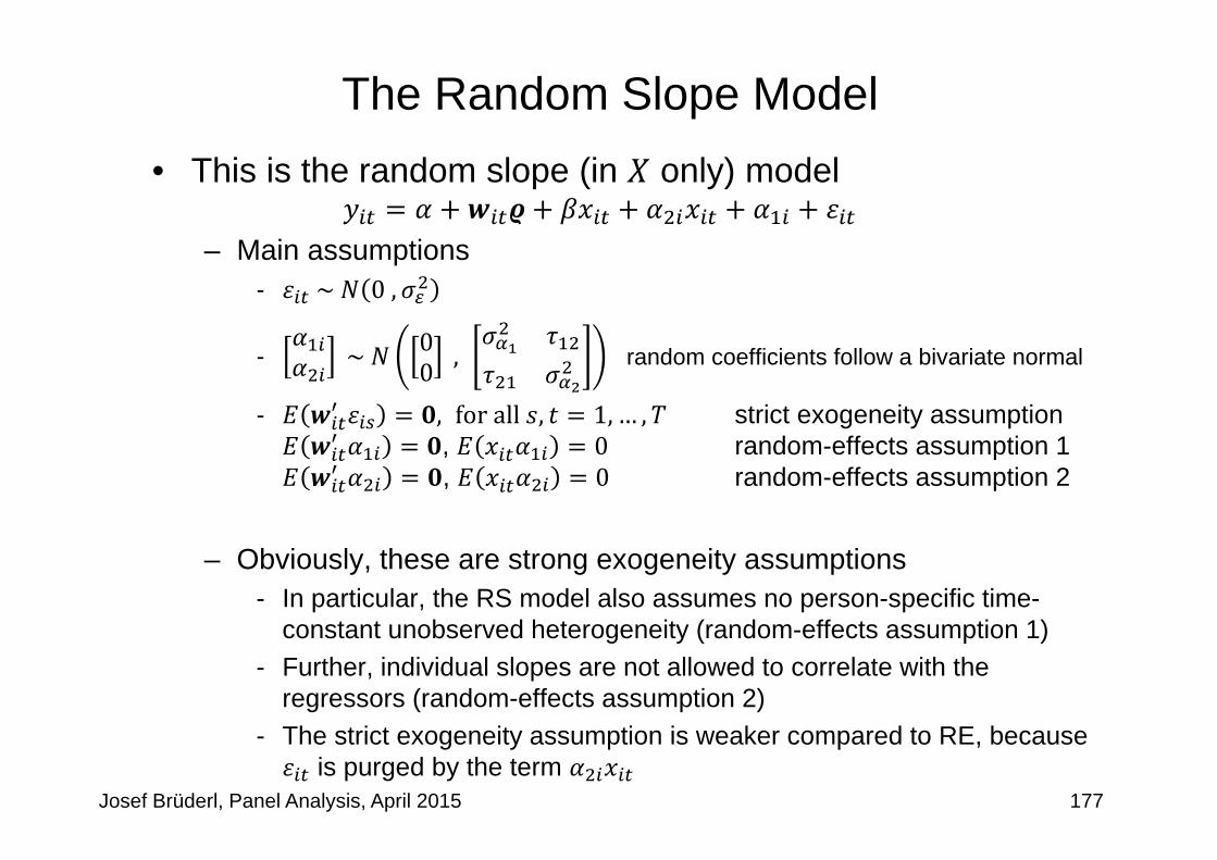
The Random Slope Model• This is the random slope (in only) model
– Main assumptions‐ ~ 0,
‐ ~ 00 , random coefficients follow a bivariate normal
‐ , forall , 1, … , strict exogeneity assumption, 0 random-effects assumption 1, 0 random-effects assumption 2
– Obviously, these are strong exogeneity assumptions- In particular, the RS model also assumes no person-specific time-
constant unobserved heterogeneity (random-effects assumption 1)- Further, individual slopes are not allowed to correlate with the
regressors (random-effects assumption 2)- The strict exogeneity assumption is weaker compared to RE, because
is purged by the term Josef Brüderl, Panel Analysis, April 2015 177

Comparing Models• Model class I
– Random intercept- Random-effect
- Fixed-effect– Fixed slope
Josef Brüderl, Panel Analysis, April 2015 178
FEIS
• Model class II– Random intercept
- Random-effect- Fixed-effect
– Random slope- Random-effect
- Fixed-effect
RS
RE/RI
FE

Comparing Models• To clarify things we compare RS with FEIS• The RS model (including time-constant )
– Here the random coefficients are assumed to be “random-effects”
• Now the FEIS model. . .
– where a “.” means that the term is not estimable– Here the random coefficients are assumed to be “fixed-effects”
• Exogeneity assumptions RS and FEIS– FEIS: , forall , 1, … ,– RS: the same plus random-effects assumptions (see above)
Josef Brüderl, Panel Analysis, April 2015 179
fixed part random part
fixed part random part

Estimation of the RS Model (“Age” random)
Josef Brüderl, Panel Analysis, April 2015 180
. mixed happy loghhinc age ||id: age, vce(cluster id) cov(unstructured) stddev
Mixed-effects regression Number of obs = 121919Group variable: id Number of groups = 14634
Wald chi2(2) = 1000.81Log pseudolikelihood = -219580.46 Prob > chi2 = 0.0000------------------------------------------------------------------------------
| Robusthappy | Coef. Std. Err. z P>|z| [95% Conf. Interval]
-------------+----------------------------------------------------------------loghhinc | .1621011 .0102715 15.78 0.000 .1419693 .1822328
age | -.0297677 .001043 -28.54 0.000 -.0318119 -.0277236_cons | 6.293142 .1075543 58.51 0.000 6.082339 6.503944
------------------------------------------------------------------------------
------------------------------------------------------------------------------| Robust
Random-effects Parameters | Estimate Std. Err. [95% Conf. Interval]-----------------------------+------------------------------------------------id: Unstructured |
sd(age) | .064252 .0015884 .0612129 .0674419sd(_cons) | 1.947417 .037498 1.875292 2.022316
corr(age,_cons) | -.8497485 .0068961 -.8627184 -.8356613-----------------------------+------------------------------------------------
sd(Residual) | 1.296047 .0062689 1.283818 1.308392------------------------------------------------------------------------------

Interpretation of the RS Model• This is a complex model, estimation takes quite long (a few min.)• There is no available here (ML model!): use Pseudo- , etc.• Fixed coefficients are interpreted as usual• What do we learn from the random coefficients?
– The coefficients are from a normal distribution with mean 0 and standard deviation sd(.)
– The fixed age slope is 0.030– The random age slopes have a s.d. of 0.064, which is significant
- “There is significant individual variation in the age slope”
– This means that 95% of the individual slopes lie within 0.03 1,96 0.064 0.156, 0.096
- Thus, there are also zero or even positive happiness GCs- We learn that the social world is complex, and that everything is possible!
Do we really want to know this?
– Random intercept and slope correlate with 0.85- The higher the intercept, the lower the slope (steeper decline)
Josef Brüderl, Panel Analysis, April 2015 181

Comparing the Models
Josef Brüderl, Panel Analysis, April 2015 182
--------------------------------------------------------------------------Variable | RE (GLS) RI (ML) RS FE FEIS
-------------+------------------------------------------------------------loghhinc | 0.1692 0.1686 0.1621 0.1323 0.0824
| 15.9416 15.8846 15.7817 10.7779 6.1668
age | -0.0251 -0.0252 -0.0298 -0.0361 | -24.4867 -24.5245 -28.5415 -23.2163
-------------+------------------------------------------------------------N | 121919 121919 121919 121919 118201
--------------------------------------------------------------------------legend: b/t
Data: Happiness2.dtaDo-File: Happiness 5 Regressions.do
• Here we focus on the income effect (“age” random-coefficient)• RE (GLS) and RI (ML) provide very similar estimates
– As it should be, because these are identical models but estimated with different methods
• The RS estimate of the income effect is similarly biased as RE– Allowing for random age slopes does not improve the estimate!– More formally you could do a LR-Test, compute BIC, etc.
• FEIS detrends the data for the individual happiness growth curves– This diminishes the income effect, because those on a less declining happiness
trajectory get more likely an income increase

Group Specific Growth Curves• Group specific GCs are often motivated within a
mixed-coefficients context– Example: sex specific GCs (male 0, female 1) [age is ]
- Consider a simple level-1 linear growth curve model
- Now the level-2 equations for the person-specific coefficients intercept group specific and random age slope group specific and random
- Plugging in gives:
- This is a RS model with sex specific GCs (RS-GC)- The RE-GC model that we estimated above is a special case with 0- Note that this model contains a so-called “cross-level interaction”
- This is a simple kind of “latent growth curve model” (LGCM)- LGCMs are usually specified in the context of SEM, and allow for even
more flexibility in modeling random coefficients, measurement errors, etc.- This easily leads to over-complex models that nobody can understand
Josef Brüderl, Panel Analysis, April 2015 183

0
1
2
3
4
5
6
7
8
Hap
pine
ss
20 30 40 50 60 70 80 90
Age
WomenMen
p p
-1.00
-0.75
-0.50
-0.25
0.00
0.25
0.50
0.75
1.00
1.25
1.50A
ME
of '
wom
an' o
n ha
ppin
ess
20 30 40 50 60 70 80 90
Age
p0
1
2
3
4
5
6
7
8
Hap
pine
ss
WomenMen
profile plot
-1.00
-0.75
-0.50
-0.25
0.00
0.25
0.50
0.75
1.00
1.25
1.50
AM
E o
f 'w
oman
' on
happ
ines
s
conditional effect plot
Happiness Example: Sex Specific RS-GCs
Josef Brüderl, Panel Analysis, April 2015 184
We compare RE-GCs (above)RS-GCs (below)
Specification: - cubic age- cohort dummies- period dummies (res.) Random slopes:- only linear age term(“this is perfectly reason-able” Rabe-Hesketh/ Skrondal, 2008: 219)Estimation of RS-GCs takes quite long (ca. 15 minutes)Results are very similar
Data: Happiness2.dtaDo-File: Happiness 5 Regressions.do

When To Use RS Models?• Raudenbush (2001) strongly advocates RS models
– He seems to be very enthusiastic about the potential of RS-GC modeling, and presents several nice examples
• However, this has to be differentiated– RS-GC models are in fact very helpful for describing personal growth
trajectories, if it is reasonable to assume that no self-selection is operating
- E.g., differences in vocabulary growth between boys and girls– However, if one wants to investigate the effects of events on
outcomes, it is likely that some sort of self-selection is going on. Then one should use FE (FEIS) methodology
- E.g., the effect of visiting a preschool on vocabulary growth• After all RS model estimates will be biased, if the strong
random-effects assumptions do not hold– Sometimes one can read statements like this: „RS models control for
unobserved heterogeneity, because they include ”– Such a statement is nonsense: RS in fact rests on a weaker strict
exogeneity assumption, however the random-effect assumptions are still very strong exogeneity assumptions
Josef Brüderl, Panel Analysis, April 2015 185

RS Exercise• Stawarz (2013)
estimates RS-GCs– Data: SOEP 1984-2009– Outcome: occupational
prestige (SIOPS)– Time: labor market
experience– GC: quadratic– RS: random intercept,
random linear and quadratic slope terms
– Controls: nationality, education parents, West, GDP, cohort and period grouped
Here are some results from his model. Might some of these results be biased due to self-selection?
186Josef Brüderl, Panel Analysis, April 2015
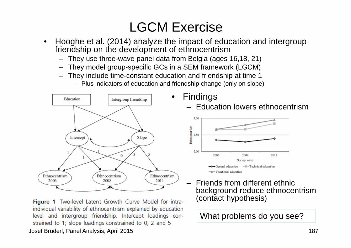
• Findings– Education lowers ethnocentrism
– Friends from different ethnic background reduce ethnocentrism (contact hypothesis)
LGCM Exercise• Hooghe et al. (2014) analyze the impact of education and intergroup
friendship on the development of ethnocentrism– They use three-wave panel data from Belgia (ages 16,18, 21)– They model group-specific GCs in a SEM framework (LGCM)– They include time-constant education and friendship at time 1
- Plus indicators of education and friendship change (only on slope)
Josef Brüderl, Panel Analysis, April 2015 187
What problems do you see?

Chapter VII: Further Linear Panel Models
Josef BrüderlApplied Panel Data Analysis
Section: The Hybrid Model

Josef Brüderl, Panel Analysis, April 2015
Hybrid Models• Hybrid models are RE-models with decomposed variables
– Hybrid- (Allison 2009), Mundlak-Model (Wooldridge 2010: pp. 332f)– Decompose each time-varying predictor into two components
- Between component: ∑ (person-specific mean)
- Within component : (demeaned variable)– Put both components into a RE-model
‐ reproduces exactly the FE estimate‐ reproduces (approximately) the BE estimate‐ is the effect of a time-constant regressor
– Within-between RE (REWB) (Bell/Jones 2015)
• The REWB is a RE model that by controlling for the between component produces within estimates plus estimates for the effects of time-constant regressors– So to say: REWB is “a correctly specified” RE model
189

Hybrid Models• Algebraically equivalent variant
– Known in the multi-level literature as
“regression with contextual variable” ( )(“contextual model”; Snijders/Bosker 1999: chap. 4.5)
– Advantage: it includes the untransformed ; one needs only one new variable (the person-specific mean)
– Disadvantage: the coefficient of is the difference of within and between effect and not interpretable
• A test of provides an alternative to the Hausman test– Advantage: one can test single parameters, whereas the
Hausman test is an overall test– If the Hybrid Model becomes the RE Model
(and RE reproduces the FE estimate)
Josef Brüderl, Panel Analysis, April 2015 190
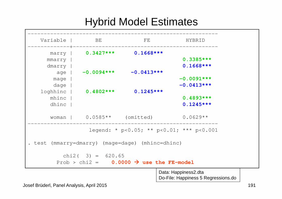
Josef Brüderl, Panel Analysis, April 2015
Hybrid Model Estimates-----------------------------------------------------------
Variable | BE FE HYBRID -------------+---------------------------------------------
marry | 0.3427*** 0.1668*** mmarry | 0.3385*** dmarry | 0.1668***
age | -0.0094*** -0.0413*** mage | -0.0091*** dage | -0.0413***
loghhinc | 0.4802*** 0.1245*** mhinc | 0.4893*** dhinc | 0.1245***
woman | 0.0585** (omitted) 0.0629** -----------------------------------------------------------
legend: * p<0.05; ** p<0.01; *** p<0.001
. test (mmarry=dmarry) (mage=dage) (mhinc=dhinc)
chi2( 3) = 620.65Prob > chi2 = 0.0000 use the FE-model
191
Data: Happiness2.dtaDo-File: Happiness 5 Regressions.do

Josef Brüderl, Panel Analysis, April 2015
Interpreting the Hybrid Model• Interpretation
– Coefficients of the within component ( ) are FE-estimates– Coefficients of the between component ( ) are “pure” between (BE)
estimates (purged from the within component)- They provide information on how much treatment and control group differ
in on average- These coefficients are (in most cases) substantively of no interest!
– Coefficients of time-constant variables ( ) are under control of both between and within components
- They are still biased, however, if correlates with
• Hybrid models confuse most researchers– Due to the presence of BE-effects that are substantively meaningless– Therefore, the hybrid is featured prominently in many panel
textbooks, but (almost) no applications exist
• If one has substantive interest in the effects of time-constant variables, use group-specific growth curves (see above)
192

Hybrid RS Model• Introducing contextual variables in an RS model
– This hybrid variant is favored by Snijders/Boskers (1999: 81)– What kind of model is this? Since is a FE estimate this is a
FE model with heterogeneous effects!- I.e. this model allows for heterogeneous causal effects‐ is an estimate of the average causal effect (ATE)‐ estimates the variation around the ATE
– The effect of the contextual variable should simply be ignored– This model further weakens the assumptions (compared to FE)
needed to get a consistent estimate of the average causal effect - [Unfortunately, I could not find the assumptions of the hybrid RS in the
literature. Generally, assumptions are underemphasized in the multi-level literature. So these are my own thoughts.]
- Random-effects assumption 1 is no longer needed- Strict exogeneity still must hold- And especially random-effects assumption 2 must hold
0i.e., there must not be a correlation between and the unobserved slope
Josef Brüderl, Panel Analysis, April 2015 193

. mixed happy mmarry marry mage age mloghhinc loghhinc woman ||id: marry, ...
Mixed-effects ML regression Number of obs = 121919Group variable: id Number of groups = 14634
Wald chi2(7) = 2687.18Log likelihood = -219936.68 Prob > chi2 = 0.0000------------------------------------------------------------------------------
happy | Coef. Std. Err. z P>|z| [95% Conf. Interval]-------------+----------------------------------------------------------------
marry | .1515053 .0215337 7.04 0.000 .1092999 .1937106age | -.041726 .0010501 -39.73 0.000 -.0437842 -.0396679
loghhinc | .1153518 .0093983 12.27 0.000 .0969315 .1337721woman | .0613625 .019987 3.07 0.002 .0221888 .1005363
...------------------------------------------------
------------------------------------------------------------------------------Random-effects Parameters | Estimate Std. Err. [95% Conf. Interval]
-----------------------------+------------------------------------------------id: Unstructured |
sd(marry) | .793625 .0207002 .7540729 .8352517sd(_cons) | 1.091112 .0084085 1.074756 1.107718
corr(marry,_cons) | -.3937819 .0227241 -.4373751 -.3483424-----------------------------+------------------------------------------------
sd(Residual) | 1.315525 .0028821 1.309888 1.321186------------------------------------------------------------------------------
Happiness Example: Hybrid RS Model
Josef Brüderl, Panel Analysis, April 2015 194
Data: Happiness2.dtaDo-File: Happiness 5 Regressions.do

Happiness Example: Hybrid RS Model• We investigate, whether there are heterogeneous marriage
effects– We include the person means (contextual variables)
- The effects of these are deleted from the output– We allow for random marriage slopes– To save computational time we do not compute panel-robust S.E.s
• Results– All effect estimates are very similar to FE
- The FE marriage effect was 0.167, here it is 0.152– However, now we see that the marriage effects are quite
heterogeneous: s.d. is 0.79- This means that 95% of the marriage effects are in the interval
0.152 1,96 0.79 1.43, 1.66– The person-specific intercepts and the marriage effects correlate
with 0.39- Happier people gain less happiness by a marriage
Josef Brüderl, Panel Analysis, April 2015 195

REWB the “Default” for Panel Analysis?• Bell and Jones (2015) argue that instead of FE, REWB should become
the default model for panel analysis– Because it provides FE estimates– Plus all the advantages of multilevel models
• In principle they are right. Some comments on their arguments:– REWB provides additionally between effects
- With individual panel data these are (mostly) substantively meaningless– REWB provides additionally effects of time-constant regressors
- In this respect, RE-GCs are much more informative– REWB allows for cross-level interactions
- These are also possible with FE (group-specific causal effects)- Unfortunately, REWB is no way around the impossibility to estimate group-specific FE-
GCs. As with FE the constant is not identified (“you can’t trick the data”)– REWB allows for heterogeneous causal effects (hybrid RS)
- Yes. But what do we do with this information (“The social world is complex and everything is possible”)?
– REWB allows for more than two levels- Yes, this is attractive if you want to do FE with more than two levels
• Thus I would argue: use FE as a “default” because it is less complex – Only if you would like to do complex modelling (heterogeneous effects, more than
two levels, context matters substantively) then REWB is an attractive modelJosef Brüderl, Panel Analysis, April 2015 196

Chapter VII: Further Linear Panel Models
Josef BrüderlApplied Panel Data Analysis
Section: Dynamic Panel Models

Correlation Over Time• Panel variables usually are correlated over time.
This can be due to two sources:– Spurious state dependence:
time-constant unobservables affect the outcomes at all times
- It follows that Corr , ,
– True state dependence:past outcomes affect “causally” future outcomes (some kind of “reproduction” / “tendency for stability”)
- Naturally modeled with a lagged dependent variable (LDV),
‐ 1 (stationary outcome process)‐ captures the amount of reproduction- If 0, it follows that Corr , ,
- [The general formula can be found in Cameron/Trivedi, 2005: 763]
Josef Brüderl, Panel Analysis, April 2015 198

• Desire to model true state dependence leads to LDV models
,
– Often termed “dynamic panel models”. - Panel models without LDV are termed “static”. These are, however,
also dynamic, because they also model time
– LDV models have “intuitive appeal” and have been the standard models for panel analysis since Lazarsfeld’s time
– Sometimes LDV models are also motivated, with the argument that the LDV captures unobserved heterogeneity
- But this is a sub-optimal approach, given that we have panel data
LDV Models
Josef Brüderl, Panel Analysis, April 2015 199

Estimating LDV Models• Introducing the LDV complicates estimation enormously!
– POLS / RE estimation is inevitably biased‐ , is necessarily correlated with , because affects the outcome
at all times. Thus estimates of are inevitably biased.- If , is correlated with (this is the case, if ) not only the
estimate of but also of will be biased (the bias of is transferred)![proofs can be found in Angrist/Pischke, 2009: chap. 5.4]
– FE estimation of LDV models does also not work!- Strict exogeneity is necessarily violated (“Nickell bias”)
(Wooldridge 2010: 290)
– Thus, one has to use instrumental variable (IV) methods - Arellano/Bond (AB) suggest using FD and , as IV (if the
“sequential exogeneity” assumption holds, lags are valid IVs).- xtabond in Stata- However, if is serially correlated (this will be the case with real data
almost always), the AB estimator is biased also
Josef Brüderl, Panel Analysis, April 2015 200

Why Is the LDV Model so Popular?• The “classical” argumentation can for instance be found in
Finkel (1995) “Causal Analysis with Panel Data”– [N.B.: Finkel (1995) terms the LDV model „static-score model“]– The FD model, „contains one highly restrictive assumption: that the
lagged dependent variable does not have an influence on either or Δ . As we will see, this assumption is likely to be incorrect.” (Finkel, 1995: 6)
- I.e., Finkel argues that there is always true state dependence– “If it is assumed that the error term in the static-score model is
uncorrelated with both and , then the coefficient can be estimated consistently through ordinary least squares (OLS) regression.” (Finkel, 1995: 11)
- He sees no special problem with the exogeneity assumption, because he does not start from an error decomposition formulation of the model. Therefore, he oversees that the error term necessarily correlates with
, if there are person-specific time-constant unobservables
Josef Brüderl, Panel Analysis, April 2015 201

Are LDV Models Useful?• Consistent estimation of LDV models seems impossible
– Simple estimation methods (POLS, FE) do not work– Even the specially developed AB method does not work
Do not use LDV models!• Further, there is no real need to use LDV models
– Often it is argued in an intuitive fashion “There is certainly some kind of reproduction going on”, but without explicating the concrete mechanisms behind it
– But state dependence in most cases will be “spurious”, produced by stable unobservables that affect the outcome at all time points
– Example: stability of wages- Caused be stable, unobserved traits: productivity, personality traits, etc.- Not by some mysterious “wage reproduction mechanism”
Josef Brüderl, Panel Analysis, April 2015 202
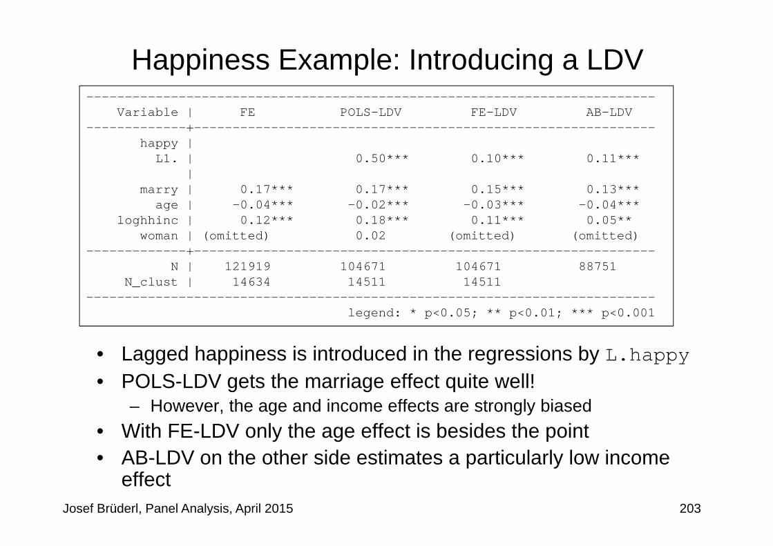
Happiness Example: Introducing a LDV
• Lagged happiness is introduced in the regressions by L.happy• POLS-LDV gets the marriage effect quite well!
– However, the age and income effects are strongly biased• With FE-LDV only the age effect is besides the point• AB-LDV on the other side estimates a particularly low income
effectJosef Brüderl, Panel Analysis, April 2015 203
--------------------------------------------------------------------------Variable | FE POLS-LDV FE-LDV AB-LDV
-------------+------------------------------------------------------------happy |
L1. | 0.50*** 0.10*** 0.11*** |
marry | 0.17*** 0.17*** 0.15*** 0.13*** age | -0.04*** -0.02*** -0.03*** -0.04***
loghhinc | 0.12*** 0.18*** 0.11*** 0.05** woman | (omitted) 0.02 (omitted) (omitted)
-------------+------------------------------------------------------------N | 121919 104671 104671 88751
N_clust | 14634 14511 14511 --------------------------------------------------------------------------
legend: * p<0.05; ** p<0.01; *** p<0.001

LDVs are Colliders• The problem in DAG notation (Morgan/Winship 2007: 71)
– In all three scenarios confounding via and – I) SD: true, no spurious
- Here the LDV blocks the confoundingpath. The LDV model works!
- Here the LDV in fact “captures unobserved heterogeneity”
– II) SD: true, spurious- But in a more realistic scenario we
also have person-specific confounders(spurious SD). Now the LDV is a collider
- If we do not control, we have confoundingIf we control, a new confounding path opens up
- We have an unsolvable dilemma!– III) SD: no true, spurious
- Here we have no problem- Only when controlling for the LDV!
Josef Brüderl, Panel Analysis, April 2015 204
YtD
Yt‐1
YtD
Yt‐1
YtD
Yt‐1

Chapter VII: Further Linear Panel Models
Josef BrüderlApplied Panel Data Analysis
Section: Comparing Models by Simulations

The Simulation Setup• Monte Carlo simulations from Brüderl/Ludwig (2015)
– Data generating process ( 200, 10),
– is a binary treatment indicator (50% treated (=1) after 5)– Scenarios:
- Heterogeneity w.r.t. : purely random heterogeneity- Selection w.r.t. : unobserved heterogeneity (levels only)- Selection w.r.t. : unobserved heterogeneity (levels and growth)- TSD: true state dependence ( 0)
Josef Brüderl, Panel Analysis, April 2015 206Source: Brüderl/Ludwig (2015)

Simulation Results
Josef Brüderl, Panel Analysis, April 2015 207Source: Brüderl/Ludwig (2015)

Simulation Results• (1) and (2): purely random heterogeneity
– Here all models are consistent; RE and RS are efficient– However, POLS-LDV is even in this innocuous situation biased,
only if there is no treatment effect (2) does this model work!• (3): selection on level
– Here only FE and FEIS work well (FE more efficient)– AB-LDV works only because there is no serial correlation in
• (4) and (5): selection on level and growth– Here only FEIS works well– Note that also RS is substantially biased, even though it allows for
individual-specific slopes (that however must not correlate with X)• (6) - (8): true state dependence
– Here only AB-LDV works, but only in the unrealistic scenarios (6, random heterogeneity) and (7, no serial correlation in )
– In the realistic scenario (8, selection and serial correlation) it is also biased. Thus under true state dependence no estimator works.
Josef Brüderl, Panel Analysis, April 2015 208

Simulations from Vaisey/Miles (2014)
Josef Brüderl, Panel Analysis, April 2015 209
• Model (scenarios (1) and (3)) 0.4– Person-specific heterogeneity , ∈ 0, 0.9
• Only FE works!– LDV doesn’t even work, if , 0

Chapter VII: Further Linear Panel Models
Section: Panel Regression with Missing Data
Josef BrüderlApplied Panel Data Analysis

Missing Data• Sources of missing data in panel data (Young/Johnson 2015)
– Unit-nonresponse in the first wave– Within-wave missingness (gap in the data)
- Item-nonresponse- Question not included in every wave
– Whole-wave missingness- Temporary unit-nonresponse (gap in the data)- Permanent unit-nonresponse (panel attrition)
• Nonresponse (NR) might bias regression estimates– If only (observable) variables affect response (MAR)– If both the treatment and the outcome affect response (NMAR)
- Endogenous selection bias (Elwert and Winship 2014)• Methods to deal with the problem (under MAR)
– Regression controlling for response variables (complete case analysis)• Methods to deal with the problem (under NMAR)
– Selection models (are not robust; “technification”)– Weighting (developed for first-wave nonresponse and attrition)– Multiple imputation (mainly for gaps, but also attrition)
Josef Brüderl, Panel Analysis, April 2015 211
YD
Response

Weighting Panel Data• With weighting one tries to compensate differential NR
– Units that are “underrepresented” in the sample get larger weights
• With panel data there are different types of weights– Cross-sectional weights (CW)
- Are constructed by adjusting a panel sample (cross-section) to population data (post-stratification weight)
- Should compensate for unit-nonresponse in the first wave- Could (in principle) be constructed also for later waves
– Longitudinal weights (LW)‐ LW where is the probability of participating in wave ‐ is estimated from a logit regression on response/nonresponse in
wave conditional on regressors from wave 1- Should compensate for permanent unit-nonresponse
– Panel weights (PW): these are finally the weights for the pyrsPW CW LW ⋯ LW
- If there is a gap: LW 1
Josef Brüderl, Panel Analysis, April 2015 212

Weighting Panel Data: ExampleYear 1 Year 2
populationA 1000 80% Surv. 800B 1000 90% Surv. 900
sampleA 50% RR 50 20% RR 10B 100% RR 100 50% RR 50
weightedsample
A 1/0.5 = 2 100 1/0.5*1/0.2 = 10 100B 1/1 = 1 100 1/1*1/0.5 = 2 100
Josef Brüderl, Panel Analysis, April 2015 213
• We draw a 10% random sample from a population. Group A has a response rate (RR) of 50%, group B has 100%. Thus the resulting sample is not “representative” of the population.
• By comparing the sample group distribution with the population distribution, we see that members of group A get the cross-sectional weight 2, group B gets weight 1
• The weighted sample is then again representative of the population• In year 2 group A has a RR of 20%, B of 50%. The respective longitudinal weights are
1/0.2=5 and 1/0.5=2. Multiplying the CWs from year 1 and the LWs from year 2 we arrive at the panel weights 10 resp. 2. Multiplying the sample with the panel weights brings the numbers back to the population distribution in year 1.
• We see, however, a drawback of this procedure: It is not guaranteed that this is representative of the population in year 2. If the population changes for instance due to mortality the weighted sample might deviate from the population.
• The problem could be solved if we would construct a new CW for year 2.

Example: Marriage and Happiness (pairfam)• In this example we replicate the SOEP results with pairfam
– We obtain very similar results
• In a next step we compare with the weighted results– As described above we compute the panel weights by multiplying up
the cross-sectional weights and the longitudinal weights
- Some panel weights are absurdly high: mean = 1.74, max = 67.3– Then we use areg to obtain an FE analysis with panel weights
- xtreg does not accept weights that change over waves– Note: pairfam provides CWs only for wave1– The CW for wave 1 is already a combination of two weights
- Post-stratification weights (comparing to Mikrozensus 2008)- Design weights (the three cohorts are not equally sized in the population)
Josef Brüderl, Panel Analysis, April 2015 214
gen pweight = dxpsweight if year==1 //W1: cross-sectional weightbysort id (year): ///W2+: multiplying the lweight(t)
replace pweight = pweight[_n-1] * lweight if year>1
areg happy marry age wave1 [pw=pweight], absorb(id) vce(cluster id)

Example: Marriage and Happiness (pairfam)
• The unweighted FE results are very similar to the SOEP results!– New is the wave1-effect:
probably due to panel-conditioning happiness was lower in wave 1
• Weighting doesn’t change the results– Coefficients change only
marginally– S.E.s are somewhat larger
(some of this increase can already be seen in the unweighted areg)
Josef Brüderl, Panel Analysis, April 2015 215
-----------------------------| FE AREG| unweight. weighted
--------+--------------------marry | 0.272 0.289
| 0.056 0.068 | 4.88 4.27
age | -0.078 -0.074 | 0.009 0.012 | -9.06 -6.40
wave1 | -0.149 -0.139 | 0.025 0.034 | -5.98 -4.09
--------+--------------------N | 27169 27169
N_clust | 6572 6572 -----------------------------
legend: b/se/t

Should we Use Weighted Regressions?• Statistical theory says “yes”• However, in practice it is unclear whether weighting really
improves our analyses– It works only well, if our weighting models are well specified– In practice, they often will be mis-specified
- Then weighted analyses might be even more biased than unweighted– Real designs are often much more complicated
- New refreshment samples and grown-up children are integrated- This complicates the construction of weights enormously- Only real experts will grasp the complexity
• Recommendation– Do not use weighted panel analysis– Only if reviewers demand it
Josef Brüderl, Panel Analysis, April 2015 216

Multiple Imputation• With multiple imputation (MI) missing values are imputed
– MI is model based where the information available is used
• There are several challenges when using MI with panel data– With within-wave item nonresponse MI should use both within-wave
and across-wave (panel) information– With whole-wave missingness we have to impute whole waves
- Time-constant variables have to be fetched forward- Timing information has to be imputed (when happened the event?)
• Simulations by Young/Johnson (2015)– MI of within-wave missingness improves FE estimates (somewhat)– MI of whole-wave missingness does not improve FE estimates
• Recommendation– As with weighting the issues involved are extremely complex and
careless usage of MI might easily increase bias– For instance, imputing time-constant variables or “not applicables”
would mess up the whole analysisJosef Brüderl, Panel Analysis, April 2015 217

Chapter VIII: Non-Linear Panel Models:
Fixed-Effects Logit
Josef BrüderlApplied Panel Data Analysis

Josef Brüderl, Panel Analysis, April 2015
Nonlinear Panel Regression• Linear model: modeling conditional means
| ,– Person-specific errors are additive, we can difference them out
• Nonlinear model: modeling conditional densities| , , ,
– Here person-specific errors can usually not be differenced out– Thus, with the parameters of interest ( , ), one has to estimate
the nuisance parameters ( , … , ), also termed incidental parameters. This creates the incidental parameter problem:
- As → ∞ the number of parameters to estimate goes to infinity, parameter estimates are inconsistent.
– Solution I: RE-estimation– Solution II: in some special cases it is possible to condition out the
nuisance parameters (conditional FE-models)
219

Josef Brüderl, Panel Analysis, April 2015
Nonlinear Panel Regression• FE-model vs. RE-model
– As in the linear case: if person-specific errors are present and are correlated with the regressors, then RE is biased but FE is consistent
– A Hausman test can be used
• Interpretation of Coefficients (see Allison 2009: pp. 36)– With nonlinear models, the coefficients of pooled and FE models
have different interpretations- Pooled models: population-averaged estimates
- Marginal effects are identical for each subject- FE (and RE) models: subject-specific estimates
- The marginal effect depends on , therefore it differs for each subject
- These are considered to be more accurate estimates of the underlying causal mechanism
220

Josef Brüderl, Panel Analysis, April 2015
Fixed-Effects Logit
• Logistic regression model with fixed-effects
1exp
1 exp– No incidental parameter problem, because the can be
conditioned out (conditional likelihood)– Advantage of the FE-methodology: Estimates of are unbiased
even in the presence of time-constant unobserved heterogeneity– Persons who have only 0s or 1s on the dependent variable are
dropped. For FE-logit you need data with sufficient variance on , i.e., generally you will need panel data with many waves!
– Subject-specific estimates: Probability interpretation not possible! One has to use the sign interpretation (or odds)
221

Josef Brüderl, Panel Analysis, April 2015
Example: Further Education0
1000
2000
3000
4000
5000
EU
RO
per
mon
th
1 2 3 4 5 6Time
no further education further education
Y: further educationX: wageDoes a wage raiseincrease P(further educ)?
The data showa) a negative effect of awage raiseb) self-selection of high wage males into further educ
222
Data: Wage Premium.dtaDo-File: Wage FE Logit.do

Josef Brüderl, Panel Analysis, April 2015
Estimation Results. replace wage = wage/1000 //wage rescaled
. * Pooled-Logit
. logit feduc wage
------------------------------------------------------------------------------feduc | Coef. Std. Err. z P>|z| [95% Conf. Interval]
-------------+----------------------------------------------------------------wage | .9478211 .4256097 2.23 0.026 .1136414 1.782001
_cons | -2.93141 1.299289 -2.26 0.024 -5.47797 -.3848511------------------------------------------------------------------------------
. * FE-Logit
. xtlogit feduc wage, fe
note: multiple positive outcomes within groups encountered.note: 1 group (6 obs) dropped because of all positive or all negative outcomes.
Conditional fixed-effects logistic regression Number of obs = 18Group variable: id Number of groups = 3
------------------------------------------------------------------------------feduc | Coef. Std. Err. z P>|z| [95% Conf. Interval]
-------------+----------------------------------------------------------------wage | -2.18767 2.32178 -0.94 0.346 -6.738276 2.362935
------------------------------------------------------------------------------
223
Data: Wage Premium.dtaDo-File: Wage FE Logit.do

Linear Probability Model as Alternative• Much easier to interpret is the LPM
– We can interpret the coefficient estimates
Josef Brüderl, Panel Analysis, April 2015 224
. xtreg feduc wage, fe
Fixed-effects (within) regression Number of obs = 24Group variable: id Number of groups = 4
R-sq: within = 0.0606 Obs per group: min = 6between = 0.9007 avg = 6.0overall = 0.2455 max = 6
F(1,19) = 1.23corr(u_i, Xb) = -0.9844 Prob > F = 0.2820
------------------------------------------------------------------------------feduc | Coef. Std. Err. t P>|t| [95% Conf. Interval]
-------------+----------------------------------------------------------------wage | -.5389222 .4866634 -1.11 0.282 -1.55752 .4796759
_cons | 1.831338 1.280712 1.43 0.169 -.8492242 4.511899-------------+----------------------------------------------------------------

Chapter IX: EHA with Repeated Events
Josef BrüderlApplied Panel Data Analysis

Josef Brüderl, Panel Analysis, April 2015
Event History Analysis with Repeated Events• Multiple episodes in the dataset
– Problem: dependent episodes, biased S.E.– Potential: within estimation
• Analysis options– Analyzing time to first event only
- Discards much information– Analyzing episodes separately
- Does not make use of the within information– Pooled estimation
- Biased S.E. and sub-optimal use of the within information– Random-effects models
- Sub-optimal use of the within information– Fixed-effects models
- Uses the within information (biased S.E., but vce() option)
226

Josef Brüderl, Panel Analysis, April 2015
Continuous-Time: Pooled- and RE-Cox• Pooled-Cox
– Pooling the data and applying Cox– Using panel-robust S.E.s (vce(cluster id))
• Proportional hazards „shared frailty“ model (RE-Cox)
exp
– person index, episode index– person-specific error term– RE-model (shared(id))
• and are correlated (under normal circumstances)– Pooled estimates and RE-estimates will be biased
227
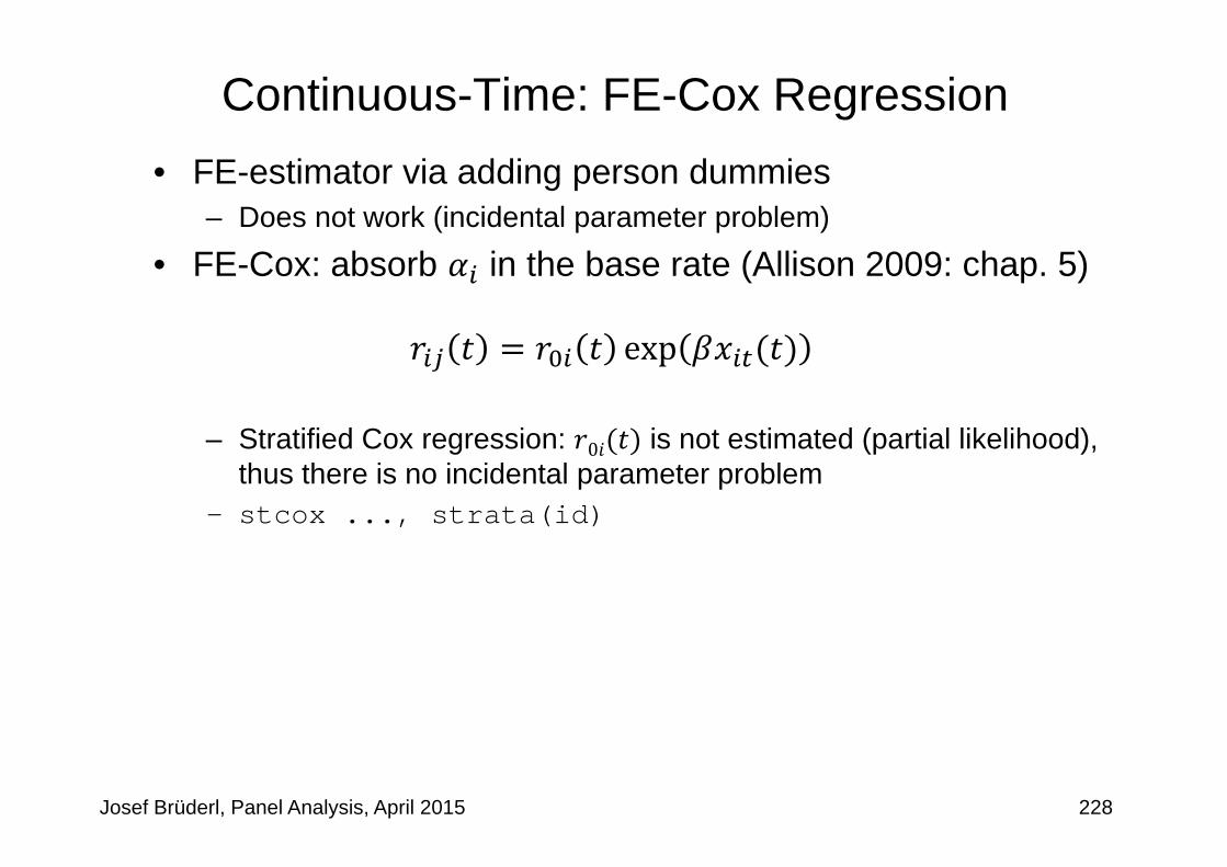
Josef Brüderl, Panel Analysis, April 2015
Continuous-Time: FE-Cox Regression• FE-estimator via adding person dummies
– Does not work (incidental parameter problem)
• FE-Cox: absorb in the base rate (Allison 2009: chap. 5)
exp
– Stratified Cox regression: 0 is not estimated (partial likelihood), thus there is no incidental parameter problem
– stcox ..., strata(id)
228
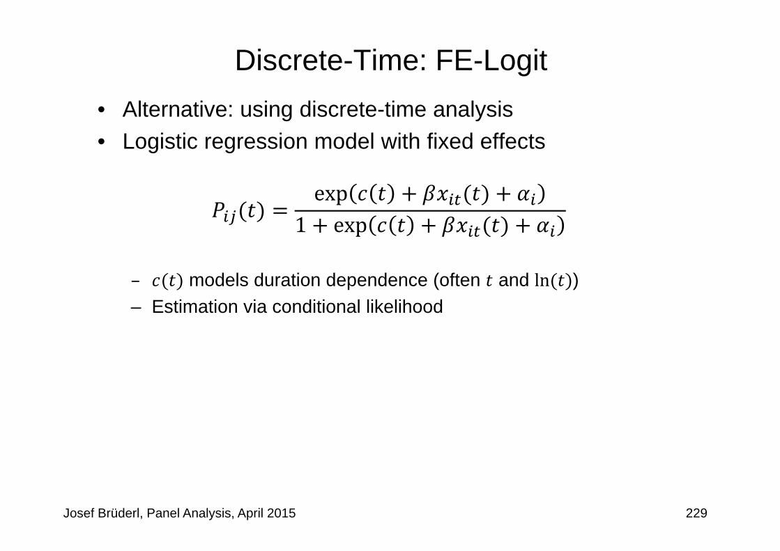
Josef Brüderl, Panel Analysis, April 2015
Discrete-Time: FE-Logit• Alternative: using discrete-time analysis• Logistic regression model with fixed effects
exp1 exp
– models duration dependence (often and ln )– Estimation via conditional likelihood
229

Josef Brüderl, Panel Analysis, April 2015
Modeling Effects of Time/History• How to define analysis time?
– Clock ticks from the first onset of the risk (elapsed time approach)– Clock is reset after each event (gap time approach)– In most situations the gap time approach will be more appropriate
• Modeling effects of history– Effect of „number of previous events“ (occurrence dependence, OD)
- Positive (spurious) OD very likely, if observation window of fixed length- FE-estimates reduce the bias
- Mechanics: is the hazard rate of episodes with a higher serial number really higher? (within persons!)
– Similar arguments for effect of “cumulative duration” or “% of life time spent in the state X”
230

Chapter IX: EHA with Repeated Events
Josef BrüderlApplied Panel Data Analysis
Example: Duration of Unemployment

Josef Brüderl, Panel Analysis, April 2015
Example: Duration of Unemployment • Data: SOEP 1984-2009 (v26)
– All unemployment episodes from ARTKALEN 1983-2008– Left-censored episodes are dropped– Event: leaving unemployment (all destinations)– Gap time approach: clock starts at 0 with every new episode– The data set:
- 10,949 respondents provide- 20,826 unemployment episodes (18,245 failures)- 230,412 month splits
– Control variables:- Time-constant: gender, living in West 1989, migration background- Time-varying: age, education, period (spring, winter, seam, 2003-06)
• Research question– What is the effect of previous unemployment on the rate of leaving
unemployment?– A negative OD is hypothesized (“scarring effect”)
232
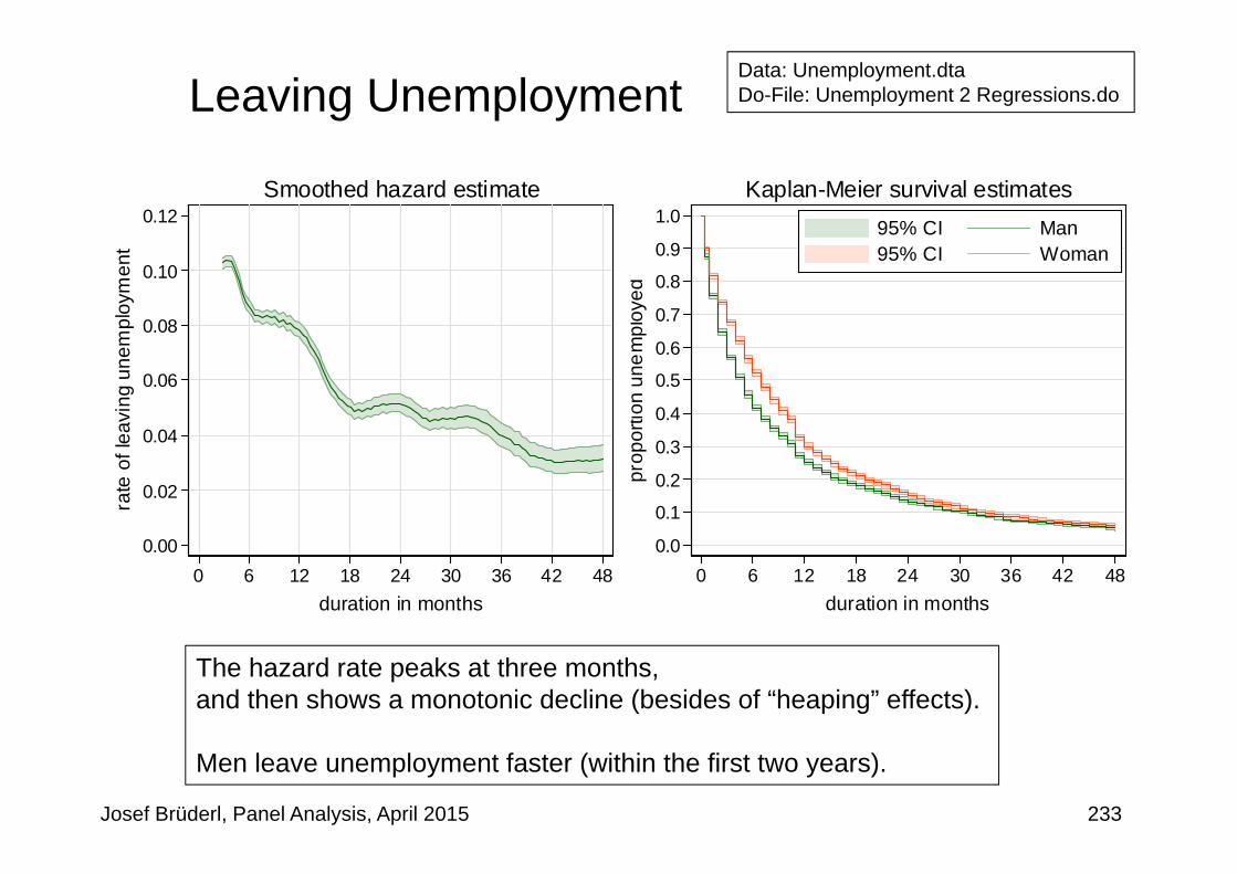
Josef Brüderl, Panel Analysis, April 2015
0.0
0.1
0.2
0.3
0.4
0.5
0.6
0.7
0.8
0.9
1.0
prop
ortio
n un
empl
oyed
0 6 12 18 24 30 36 42 48duration in months
95% CI Man95% CI Woman
Kaplan-Meier survival estimates
Leaving Unemployment
0.00
0.02
0.04
0.06
0.08
0.10
0.12
rate
of l
eavi
ng u
nem
ploy
men
t
0 6 12 18 24 30 36 42 48duration in months
Smoothed hazard estimate
The hazard rate peaks at three months, and then shows a monotonic decline (besides of “heaping” effects).
Men leave unemployment faster (within the first two years).
233
Data: Unemployment.dtaDo-File: Unemployment 2 Regressions.do

Josef Brüderl, Panel Analysis, April 2015
FE-Cox Resultsstcox nprev age educ spring winter seam y0306, strata(id) efron vce(cluster id)
Stratified Cox regr. -- Efron method for ties
No. of subjects = 17655 Number of obs = 200448No. of failures = 15616Time at risk = 200448
Wald chi2(7) = 415.87Log pseudolikelihood = -8143.5372 Prob > chi2 = 0.0000
(Std. Err. adjusted for 9171 clusters in id)------------------------------------------------------------------------------
| Robust_t | Haz. Ratio Std. Err. z P>|z| [95% Conf. Interval]
-------------+----------------------------------------------------------------nprev | .9068937 .0155766 -5.69 0.000 .8768722 .937943
age | .9919157 .0064574 -1.25 0.212 .9793398 1.004653educ | 1.023851 .0259907 0.93 0.353 .9741568 1.076081
spring | 1.226209 .0426469 5.86 0.000 1.145408 1.31271winter | .6272161 .0281982 -10.38 0.000 .5743137 .6849915seam | 1.226957 .0612777 4.10 0.000 1.112546 1.353134
y0306 | .8353965 .0347889 -4.32 0.000 .7699199 .9064414------------------------------------------------------------------------------
Stratified by id
We see negative OD (“scarring”)
234
Data: Unemployment.dtaDo-File: Unemployment 2 Regressions.do

Josef Brüderl, Panel Analysis, April 2015
Comparing Models for Repeated Events---------------------------------------------------------------------Variable| Pooled Cox Pooled Logit FE-Cox FE-Logit --------+------------------------------------------------------------
nprev | 1.01 1.01 0.91*** 0.81*** # previous unempl. epis.age | 0.98*** 0.97*** 0.99 0.99 age in years
female | 0.83*** 0.81*** femalewest | 1.11*** 1.13*** living in West 1989
migrant | 0.79*** 0.77*** migration backgroundeduc | 1.07*** 1.08*** 1.02 1.11*** education in years
spring | 1.31*** 1.36*** 1.23*** 1.33*** February, March, Aprilwinter | 0.69*** 0.67*** 0.63*** 0.64*** November, January
seam | 1.68*** 1.90*** 1.23*** 1.83*** Decembery0306 | 0.82*** 0.80*** 0.84*** 0.70*** period 2003-2006
t | 0.99*** 1.00 lnt | 0.90*** 2.19***
_cons | 0.15*** --------+------------------------------------------------------------
N | 200448 200448 200448 181233 SplitsN_sub | 17655 17655 17655 Episodes
N_fail | 15616 15616 15616 FailuresN_g | 9171 9171 9171 7613 Persons
---------------------------------------------------------------------legend: * p<0.05; ** p<0.01; *** p<0.001
All models with panel-robust S.E.s (FE-Logit with bootstrap)FE-Cox keeps only persons, where a within comparison is possible (not seen in the output)
a) at least two failures, b) one failure plus at least one censor: censored duration >= failure duration
Contrary, the FE-Logit includes also persons with only one failure episodeIt drops all persons with only 0s (or only 1s)
235

Josef Brüderl, Panel Analysis, April 2015
A Caveat on Estimating OD Effects• A standard EHA model (pooled or RE-analysis) will provide
upwardly biased OD estimates– In a fixed observation interval, subjects with more episodes will have
(ceteris paribus) shorter durations (higher rates)– OD will be spuriously positive
• A FE-approach is not prone to this bias– Within subjects one looks, whether durations increase with the serial
number of the episode (if yes: negative OD)– However, there might be a bias in the opposite direction
- Chamberlain (1985) argued that censoring is no longer independent- Allison (1996) showed with simulations that there is a potential for a
negative OD bias (also for “cumulative duration dependence”)- Especially severe if few episodes per subject
(and/or many censored episodes)– Take negative OD found in FE-models also with caution!
236

Chapter X: Limitations of the Within Methodology
Josef BrüderlApplied Panel Data Analysis
Section: Limitations of Scope

Limitations of the Within Methodology• The main point with FE is that it discards potentially
“contaminated” between variation (Allison 2009) – It uses only within variation to estimate the causal effect of an event – Thus, to identify the causal effect FE needs only the assumption that
the within variation is exogenous
• Several implications follow:1) FE can only be applied, if there is within variation.2) For descriptive purposes it makes sense to use also the between
variation.3) Because the FE estimator uses only the within variation, it is only
generalizable to those units that show within variation, i.e. it is an ATT.
4) If the within variation is not exogenous the FE estimator will yield biased estimates.
Josef Brüderl, Panel Analysis, April 2015 238

Is There Enough Within Variation?• FE identifies the causal effect by using within variation only
– Therefore, one has to ask for every variable of interest- whether there are enough changes? (categorical variables)- whether there is enough within variation? (metric variables)
• Example: education– When investigating the effects of human capital on wages, it is
difficult to use within methodology, because education does not change during the labor market career of most people
• Sometimes there is also „meaningless“ within variation– Throwing a “raw” sex variable in a FE model, usually will provide a
FE estimate, because there are sex changes in panel data due to measurement errors. Such an estimate is obviously meaningless.
– Therefore, most panel data providers deliver a “consolidated” sex variable that is constant over waves.
Josef Brüderl, Panel Analysis, April 2015 239

Descriptive Questions• In Social Sciences descriptive questions are also important
– Some even argue that we first should have good descriptions of the social world, before we start with analyzing causal effects
• For descriptive questions one has to use between variation– FE describes effects of events, it does not describe group differences– For describing group differences use POLS
- Not RE, because RE is „biased“ towards FE- In fact, panel data are sub-optimal for this purpose.
Trend data would be better for describing group differences!
• Examples – What is the earnings difference between East and West Germans?
What is the causal effect on earnings of moving from West Germany to East Germany?
– What is the wage differential between large and small firms? What is the causal effect on wages of moving from a large to a small firm?
Josef Brüderl, Panel Analysis, April 2015 240

Within Methods Provide Only ATTs• When estimating causal effects, one always has to ask, what kind of
treatment effect do I identify?– An „average treatment effect“ (ATE) that generalizes to the whole population– Or an “average treatment effects on the treated” (ATT) that generalizes only to
those, who potentially can experience the treatment• Within estimators identify an ATT
– They use only within variation of those, who experienced an treatment– Therefore, we can only generalize to those, who potentially can/will experience
the treatment• For causal analysis ATTs are preferable
– The „Not Treated“ could have a completely different treatment effect (effect heterogeneity) (ATC). Perhaps this is even the reason why they did not choose treatment. Therefore, the ATE is „biased“ by the ATC
– Contrary, the ATT is what one wants: „what is the effect of a treatment, on those who will experience that treatment“?
– In experiments we „force“ some subjects into treatment, who under „natural“ conditions never would have taken the treatment. Thus, an experiment identifies an ATE
– However, policy measures should be based on ATEs, because with a policy measure one usually wants to „force“ some subjects into treatment, who under „natural“ conditions never would have taken the treatment
Josef Brüderl, Panel Analysis, April 2015 241

Within Methods Provide Only ATTs• Example: marriage premium
– Estimating the wage difference between married and unmarried people (by POLS) generalizes to the whole population. However, this is not a treatment effect, it is only a descriptive group difference
– The marriage premium estimated with FE generalizes only to those, who eventually will marry. It does not apply to „hard-core-singles“
– The latter may even stay single, because for them the treatment effect is completely different (i.e., a negative marriage premium)
– In an experiment some „hard-core-singles“ would be „forced“ to marry. Therefore, the experiment will provide an ATE
– Imagine we found a positive ATT: It is not guaranteed that policy measures introduced to increase marriage would rise the wage level
• Example: sex change– Sometimes one observes enough true sex changes. Applying FE to
such data provides an ATT for transsexuals only
Josef Brüderl, Panel Analysis, April 2015 242

Chapter X: Limitations of the Within Methodology
Josef BrüderlApplied Panel Data Analysis
Section: Violations of Strict Exogeneity

Josef Brüderl, Panel Analysis, April 2015
Endogeneity
• FE estimates are biased under endogeneity: , forsome , 1, … ,
• Note that endogeneity can have several sources– Unobserved time-varying confounders– affects also (reverse causality, simultaneity)– Errors in reporting X (measurement errors)– Endogenous selection bias (collider bias, attrition) [see next section]
• Endogeneity thus is the consequence of substantive mis-specification or methodological deficiencies– When arguing for exogeneity, one has to make it plausible, that
none of the four sources is at work
244

Unobserved Time-Varying Confounders• Unobservables that affect both and
– So far we assumed that the red arrow does not exist– However, there might be plausible arguments for such an arrow
- For instance, a cosmetic surgery could affect contemporaneous or future chances for marriage
- Or past (non) marriage could affect cosmetic surgery.
• Time-varying unobservables can produce non-parallel trends
Josef Brüderl, Panel Analysis, April 2015 245
wagemarriage
cosmeticsurgery

Measurement Errors• In a bivariate regression, measurement errors generally
produce an “attenuation bias”– With more X-variables the direction of the bias is unknown
• Within estimators increase the problem– In fact, compared with pooled-OLS the bias due to measurement
errors is amplified by using FD- or FE-estimators, because taking the difference of two unreliable measures generally produces an even more unreliable measure
– On the other hand, pooled-OLS suffers from bias due to unobserved heterogeneity
– Simulation studies show that generally the latter bias dominates– The suggestion is, therefore, to use within estimators: unobserved
heterogeneity is a "more important" problem than measurement error.
Josef Brüderl, Panel Analysis, April 2015 246

010
0020
0030
0040
0050
00EU
RO
per
mon
th
1 2 3 4 5 6Time
before marriage after marriage
Example for Measurement Errors
Josef Brüderl, Panel Analysis, April 2015 247
The highest earner reported marriage one year too late.Now FE is biased, but POLS is still biased much more!
. regress wage marr1------------------------------------------------------------------------------
wage | Coef. Std. Err. t P>|t| [95% Conf. Interval]-------------+----------------------------------------------------------------
marr1 | 1610.526 556.2303 2.90 0.008 456.9754 2764.077_cons | 2289.474 253.8832 9.02 0.000 1762.952 2815.995
------------------------------------------------------------------------------
. xtreg wage marr1, fe------------------------------------------------------------------------------
wage | Coef. Std. Err. t P>|t| [95% Conf. Interval]-------------+----------------------------------------------------------------
marr1 | 441.1765 72.57272 6.08 0.000 289.28 593.0729_cons | 2533.088 29.16108 86.87 0.000 2472.053 2594.123
-------------+----------------------------------------------------------------

Simultaneity• Reverse causality: → Simultaneity: ⇄• An important case of simultaneity are feedback mechanisms
– The covariates might react to shocks on the outcome→ →
– Then , will correlate with – Note that this violates strict exogeneity but not sequential exogeneity!
- In this situation FD is not biased!!
• Examples of feedback mechanisms– Question: Is there a male marital wage premium?
- Men get a job promotion plus more wage, and then marry– Question: Does a new coach increase performance of soccer teams?
- The performance of a soccer team gets worse, and therefore it hires a new coach
• Robustness check– Compare FE and FD estimates. If they differ there might be feedback– Problem: “feedback” is statistically not distinguishable from “anticipation”
- We need substantive knowledge to decide what is going onJosef Brüderl, Panel Analysis, April 2015 248

Josef Brüderl, Panel Analysis, April 2015
Example for Feedback Mechanism
Modified Data:
The wage jump at 3triggers marriage, i.e., causality runs the other way.
There is no additional causal effect of marriage!
There is still selectivity.
010
0020
0030
0040
0050
00E
UR
O p
er m
onth
1 2 3 4 5 6Time
before marriage after marriage
249
Data: Wage Premium.dtaDo-File: Wage Premium.do

Josef Brüderl, Panel Analysis, April 2015
Example for Feedback Mechanism
• Now the FE estimator is biased• The FD-estimator provides the correct answer!
– Substantive knowledge tells us that this is probably feedback not anticipation• Another idea for solving the problem with feedback
– Synthetic control group method (SCM)– DID-matching on panels (life courses) before treatment occurs– I.e., match men that get also a wage increase but do not marry
. xtreg wage2 marr, fe------------------------------------------------------------------------------
wage2 | Coef. Std. Err. t P>|t| [95% Conf. Interval]-------------+----------------------------------------------------------------
marr | 350 88.27456 3.96 0.001 165.2392 534.7608_cons | 2575 38.22401 67.37 0.000 2494.996 2655.004
-------------+----------------------------------------------------------------
. regress D.(wage2 marr), noconstant------------------------------------------------------------------------------
D.wage2 | Coef. Std. Err. t P>|t| [95% Conf. Interval]-------------+----------------------------------------------------------------
D1.marr | 0 128.7593 0.00 1.000 -269.4962 269.4962------------------------------------------------------------------------------
250
Data: Wage Premium.dtaDo-File: Wage Premium.do

Simulations from Vaisey/Miles (2014)
• Model 0.4– Person-specific heterogeneity , 0.5– Simultaneity
• None of the estimators works!– If there is no reverse causality ( 0) FE works
Josef Brüderl, Panel Analysis, April 2015 251

Endogeneity: What to Do?• If endogeneity is due to non-parallel trends then use FEIS• The standard suggestion is to use complex statistical models
– Instrumental variables (IV) estimation (xtivreg)- FD-IV and FE-IV are available.- If “sequential exogeneity” is maintainable,
then FD-IV can use the lagged regressors as a valid instrument– Structural equation modeling (LISREL)
- LISREL models supposedly can take regard of simultaneity and measurement errors
– Problems of these methods- They rest on untestable assumptions- They are not robust
Research fields that use these methods abundantly are full of contradictory results. These methods have produced a big mess in social research. Be very careful, when using them.
Josef Brüderl, Panel Analysis, April 2015 252
wagemarriage
tenure

Endogeneity: What to Do?• Traditionally, it has been believed that more complex
methodology equals better research (“technification”)• More and more social researchers are convinced that
social research should not invest in ever more complex statistical methods– “Those who worship at the altar of complex methods are prone to
the error of thinking that technical sophistication can substitute for knowledge of the subject matter, careful theorizing, and appropriate research design” (Firebaugh 2008: 207f)
– “We cannot rely on statistical wizardry to overcome faulty data and research design” (Firebaugh 2008: 208)
– Keep it simple: Generally complex statistical models will not make your inferences better
Josef Brüderl, Panel Analysis, April 2015 253

Alternatives to Technification• Be critical!
– If you have doubts on the validity of the strict exogeneity assumption, be careful when interpreting FE results
– Use IV methods only, when you have good arguments for the validity of the instruments used
– If you find no good IV, be conservative and conclude that even the panel data at hand do not help in identifying the causal effect
• Invest in “shoe leather”– Invest in better research design
- Try to collect better data (panel data) that include (i) the time-varying unobservables, and (ii) more precise measures
- Try to collect better data by (natural) experiments
Josef Brüderl, Panel Analysis, April 2015 254

And: Always Discuss Your Assumptions!• An essential lesson from the “new wave of causal analysis”
is that you always should discuss the plausibility of the assumptions that you need to identify the causal effect– Might there be endogeneity?
• Example: marriage and happiness– Time-varying unobservables
- We did certainly not control for some obvious candidates: E.g., birth of a (first) child
– Feedback mechanisms- It doesn’t seem plausible that a positive happiness shock triggers
marriage. It is more plausible that we see an anticipation effect.
– Measurement errors in - We see no obvious problems with “hard facts” as used here- Males more often misreport family events.
Robustness check: estimate models with females onlyJosef Brüderl, Panel Analysis, April 2015 255

Chapter X: Limitations of the Within Methodology
Josef BrüderlApplied Panel Data Analysis
Section: Consequences of Panel Attrition

Panel Attrition• Panel attrition is seen as a major threat to panel analyses
– This assertion has to be qualified: attrition is not always a problem! – Case I) Attrition produced by (unobservable) regressors only
- FE estimation offers some advantages here! Attrition correlated with does not bias FE estimates (cf. Wooldridge 2010: 837ff)!
- I.e., attrition associated with person-specific characteristics (observed or unobserved!) does not bias FE estimates
- FEIS is even more robust (allowing for attrition correlated with het. trends)– Case II) The treatment and the outcome affect response (NMAR)
(endogenous selection bias, Elwert and Winship 2014)- This produces endogeneity and the
FE estimates will be biased also
• What can we do in case II?– There are special attrition selection models,
there is weighting and imputation- But this is technification!
– However, there is an obvious robustness check- Restrict analysis to only those observed continuously. If results remain,
then it is unlikely that attrition biased the results257
YD
Response
Josef Brüderl, Panel Analysis, April 2015

Attrition Biases Impact Functions• If there is effect heterogeneity, attrition might bias results
– If effect strength is connected with the probability of attrition then those observed for a long time under treatment are a select sample
– This will bias the impact function
• Example: Step impact function– Those observed longer after treatment get a higher weight in FE
estimation
• Example: Modeling the marriage effect with a dummy impact function [see next slide]– Assume a constant marriage impact– But those, with a larger marriage impact stay longer married– Then it will appear, as if the marriage effect increases with
marriage duration- At higher marriage ages only those with the larger effects are left
Josef Brüderl, Panel Analysis, April 2015 258
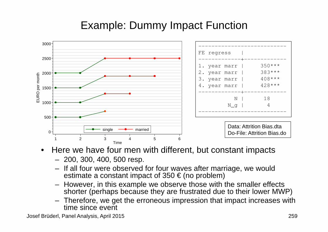
0
500
1000
1500
2000
2500
3000E
UR
O p
er m
onth
1 2 3 4 5 6Time
single married
Example: Dummy Impact Function
• Here we have four men with different, but constant impacts – 200, 300, 400, 500 resp.– If all four were observed for four waves after marriage, we would
estimate a constant impact of 350 € (no problem)– However, in this example we observe those with the smaller effects
shorter (perhaps because they are frustrated due to their lower MWP)– Therefore, we get the erroneous impression that impact increases with
time since eventJosef Brüderl, Panel Analysis, April 2015 259
---------------------------FE regress | -------------+-------------1. year marr | 350*** 2. year marr | 383*** 3. year marr | 408*** 4. year marr | 428*** -------------+-------------
N | 18 N_g | 4
---------------------------
Data: Attrition Bias.dtaDo-File: Attrition Bias.do

Chapter X: Limitations of the Within Methodology
Josef BrüderlApplied Panel Data Analysis
Section: Consequences of Panel Conditioning

Panel Conditioning• Next to attrition, panel conditioning is the second
methodological problem that might bias panel analyses– If respondents react to measurement this might produce
- Response effects (measurement errors)- Or even behavioral change
• The methodological literature is ambivalent on whether panel conditioning exists– Response effects can be found occasionally– Behavioral change has not been found
• Example: happiness (Kratz/Brüderl 2015)– Over the first three waves, SOEP respondents adapt their
happiness responses– Such a response effect can easily be controlled by wave dummies
- 1.wave: +0.28*** 2.wave: +0.10*** 3.wave: +0.04***- Works only in a multi-cohort, multi-subsample panel like the SOEP
Josef Brüderl, Panel Analysis, April 2015 261

Chapter X: Limitations of the Within Methodology
Josef BrüderlApplied Panel Data Analysis
Section: Direction of Causality

Direction of Causality• It is often asserted that from panel data we can learn about
the direction of causality → ,or ← ,or ⇄
• This assertion has to be qualified, however– If investigating the effects of events we can construct our data so
that the treatment comes before the outcome - Thus with panel data it is possible to establish the correct time-ordering
of cause and effect. This is very helpful for causal analysis- This has been described in Chap. V
- Nevertheless, even in this situation we have problems, if there are anticipation effects. Then the panel data alone do not tell us whether we see anticipation or feedback effects (reverse causality)
- This has been discussed above– It is even more ambitious to establish the causal ordering of two
continuous variables- The models used for this are inherently problematic (see next slides)
Josef Brüderl, Panel Analysis, April 2015 263

Lagged First-Difference Model (LFD)• An intuitive idea for establishing causal ordering is to
include lagged regressors in FE models,
– This model seems (i) to protect the researcher against unobserved heterogeneity bias, and (ii) to establish causal ordering
– Allison (2009: 94) is very enthusiastic about such models• Even less assumptions are needed for the estimation of a
lagged first-difference model (LFD) (Vaisey/Miles 2014), , , ,
– This model assumes that a change in X between two waves affects Y between the following waves
- I.e., it assumes a causal lag of one wave– Lag length is determined by the spacing of waves (“data lag”)
- E.g., with yearly spaced waves the data lag is one year– The real process might have a different lag length (“process lag”)
- If the “process lag” differs from the “data lag”, LFD might not work!
Josef Brüderl, Panel Analysis, April 2015 264

Simulating LFD• Allison (2009: 95) asserts that LFD does a good job in
recovering the correct parameters. However, his simulations generate the data by a process with lags matching the spacing of data collection.– I.e., “process lag” and “data lag” coincide
• Vaisey/Miles (2014) simulations are more realistic– Their simulations show a bias towards the opposite sign of the true
effect ( )– This is the case if the “process lag” is shorter than the “data lag”
[and this is probably the situation with most annually collected panel data!]
– Therefore, most applications of the LFD will provide artificial negative effects! (if the true effect is positive)
• The lesson is that panel data help only in identifying the direction of causality if the waves are spaced according to the process lag
Josef Brüderl, Panel Analysis, April 2015 265
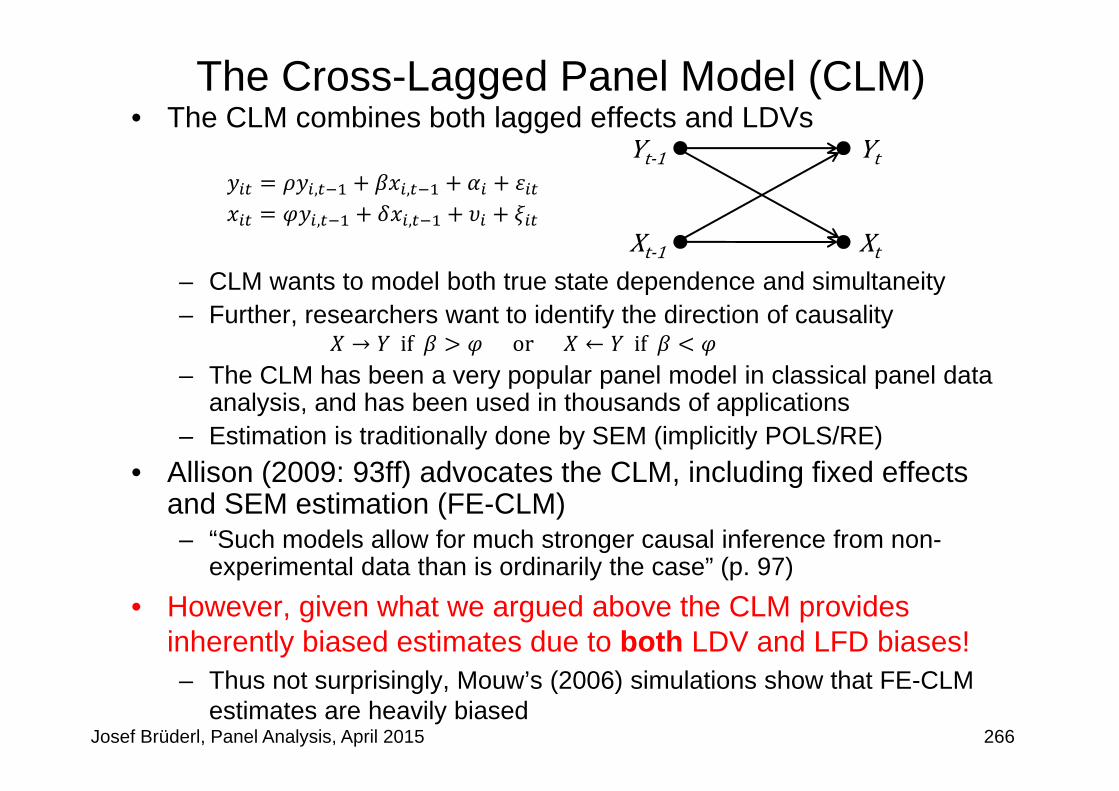
The Cross-Lagged Panel Model (CLM)• The CLM combines both lagged effects and LDVs
, ,
, ,
– CLM wants to model both true state dependence and simultaneity – Further, researchers want to identify the direction of causality
→ if or ← if– The CLM has been a very popular panel model in classical panel data
analysis, and has been used in thousands of applications– Estimation is traditionally done by SEM (implicitly POLS/RE)
• Allison (2009: 93ff) advocates the CLM, including fixed effects and SEM estimation (FE-CLM)– “Such models allow for much stronger causal inference from non-
experimental data than is ordinarily the case” (p. 97)• However, given what we argued above the CLM provides
inherently biased estimates due to both LDV and LFD biases!– Thus not surprisingly, Mouw’s (2006) simulations show that FE-CLM
estimates are heavily biasedJosef Brüderl, Panel Analysis, April 2015 266
YtYt‐1
XtXt‐1

Chapter XI: Final Remarks on Panel Analysis
Josef BrüderlApplied Panel Data Analysis
Section: Panel Regression and Causal Inference

Causal Inference• We want to identify the causal effect of a
binary treatment variable on the outcome variable
– Note: For establishing a causal effect it needs two things 1. Establishing convincing empirical evidence for an association of and 2. Providing convincing theoretical arguments for the intervening causal
mechanisms that produce this association
• The fundamental problem of causal inference– An individual causal effect is defined as:
– However, in the “real world” a unit cannot be observed both in treatment ( 1) and control ( 0) at the same time
– So we have to compare different units– Depending on how the units are assigned to treatment and control,
one needs different assumptions for identifying the causal effect
Josef Brüderl, Panel Analysis, April 2015 268
YD

Fundamental Problem of Social Research• Randomized assignment (experiment)
– Assignment is exogenous– All variation observed in is exogeneous and can therefore be used to
identify the causal effect– The causal effect can simply be inferred from the mean difference in
treatment and control group (NATE)• In social research experiments are often not practicable. We
mostly rely on non-experimental (observational) data• This creates a fundamental problem:
Due to self-selection treatment assignment is endogenous – Human beings decide according to their characteristics (or even the
value of ), whether they go into treatment or not– Therefore, the NATE is a biased estimate of the causal effect– Depending on the exact assignment mechanism, different approaches
to causal analysis are needed- Selection on observables- Selection on unobservables
Josef Brüderl, Panel Analysis, April 2015 269

Selection on Observables– Treatment assignment by observed confounder
- The variation in is endogenous, i.e., there is a spurious common variation between and induced by the confounder
– Identifying assumption: conditional independence (CIA)- After conditioning for , variation in is exogenous again
– Approaches available:- Stratification by (sub-group analysis)- Partialing out (regression)- Balancing (matching)
• In a regression framework:
- Exogeneity assumption E | 0 is violated, because is part of – The problem disappears, if one conditions (controls) for
- Now the exogeneity assumption E | , 0 is valid This fundamental insight spurred the “age of regression”
Josef Brüderl, Panel Analysis, April 2015 270
Y
V
D
Z

Selection on Unobservables• Selection on Unobservables
– Treatment assignment by observables and unobservables – Even after conditioning for , treatment assignment is endogenous
- There is common variation in and induced by the unobservables
• The modern consent: selection on unobservables is ubiquitous in non-experimental social researchMost treatment variation available is endogenousMany (most?) standard regression results are biased!
Josef Brüderl, Panel Analysis, April 2015 271
Y
U
D
Z

Identifying Strategies under Selection on Unobservables• Basically there are two possible strategies available
– “Technification” (complex statistical modelling)- E.g., structural equation modelling (SEM)
– Better Research Design- Front-door conditioning (mechanisms based causal analysis)
- Measure the intervening variables- Search for exogeneous variation in
- Instrumental variables approach (IV)» Search for an IV that is correlated with , but not with . Then
the variation in that is produced by the IV is exogenous- Regression discontinuity approach (RD)
» Look for an exogenous threshold were similar units are selected into treatment and control. Comparing these near-threshold units identifies the causal effect
- Fixed-effects approach (FE)» Look for within variation induced by an
(hopefully) exogenous treatment- The common strategy: by eliminating the endogenous (“contaminated”)
variation, we (hopefully) are left with exogeneous variation only!
Josef Brüderl, Panel Analysis, April 2015 272

In Search for Exogenous Variation: FE• If treatment assignment is produced by unobservables
– There is common variation in and that is induced by the unobservables‐ is endogenous (spurious correlation)
– Identifying strategy: use the within variation in that is not affected byperson-specific confounders- By applying the within transformation one wipes out
- Only within variation is left- By using the within variation only, we can
then identify the causal effect» FE: POLS with the demeaned data
– Main identifying assumption: strict exogeneityE | 0
- In many situations this assumption will be reasonable
Josef Brüderl, Panel Analysis, April 2015 273
demeaned data: , etc.

Chapter XI: Final Remarks on Panel Analysis
Josef BrüderlApplied Panel Data Analysis
Section: The FE Revolution in Social Research

The FE Revolution in Social Research• Panel data and the use of FE methodology have
shattered many seemingly well established facts– Above we have seen several examples– Here I will collect further examples from the literature
275Josef Brüderl, Panel Analysis, April 2015

Kroh, M. (2013) Unequal Political Voice and Family Background. Unpublished manuscript.

277
Political Engagement• Political engagement
– Hundreds of studies have shown that people with higher income show more political engagement
- However, there is good reason to suspect that this result is biased due to time-constant unobserved heterogeneity
- Particularly, there may be family unobservables that make kids more active citizens and provide the basis for better labor market positions (e.g., some kind of family “habitus”, genetic transmission of cognitive and non-cognitive skills)
– Data: SOEP and BHPS- Outcome: four point-scale measuring the amount of involvement in a
citizens' group, political party, local government and volunteer work in clubs or social services
– Kroh replicates the conventional result when using POLS– However, by using FE panel and siblings models he shows that an
increase in income has the opposite effect- With an income increase political engagement actually declines!
Josef Brüderl, Panel Analysis, April 2015

Results
278
Source: Kroh 2013
– Between family:between regression on family means (e.g., you compare the average engagement of families with different average incomes)
– Within family:family FE regression (e.g., you compare the engagement of siblings with different incomes)
– Within individual:panel FE regression (e.g., you compare the engagement of a person before and after income changes)
• Results: between regression shows strong positive effects that vanish or even become negative when using within approaches
• SOEP results on political engagement
Josef Brüderl, Panel Analysis, April 2015

Kratz, Fabian and Josef Brüderl (2013) Returns to Regional Migration: Causal Effect or Selection on Wage Growth? Schmollers Jahrbuch 133: 227-238.

Returns to Regional Migration• Standard migration theory
– People move, because they will get higher wages– Thus, we will observe positive returns of migration
• Selection on wage level– It is predominantly the “underpaid” people that move– Therefore, POLS will underestimate the returns to migration– FE estimates will be unbiased
• Selection on wage growth– Some argue, that it is especially the motivated who move,
and those are on a steeper wage trajectory– FE estimates are biased upwards, FEIS estimates will be lower
• Our research questions– Are FE estimates of the returns to migration biased, due to
selection on wage growth? – What are the “true” returns (FEIS)?
Josef Brüderl, Panel Analysis, April 2015 280

Data and Research Strategy• SOEP v27 (1984-2010)• Outcome
– Deflated log. hourly wages
• Definition of regional migration – Household lives in a new flat, due to “job related reasons”– Model I: Dummy– Model II: Dummy + years since migration + (years since migration)2
• Controls: – Firm tenure– Years of education– Currently enrolled in higher education– GDP growth rate (period dummies)
• To get unbiased estimates we use FEISln
Josef Brüderl, Panel Analysis, April 2015 281

Sample Restrictions• Sample restrictions
– Men, who live in West-Germany when first observed– Working at least 19 hours per week– Earning more than 1 € per hour
• This leaves 1711 first moves, and 399 second+ moves– We restrict our analyses to first moves only
- Panels are censored, if a second move occurs– Person years with missings on at least one model variable are
dropped– Persons migrating in the first person year are dropped– Persons with less than four person years are dropped
• We end up with 523 first moves– Control group (stayers): 7603
Josef Brüderl, Panel Analysis, April 2015 282

Comparing Models
Josef Brüderl, Panel Analysis, April 2015 283
• POLS: 2.4 % biased downwards, because the underpaid migrate• FE: 6.8 % biased upwards, because the more motivated migrate• FEIS: 2.9 % unbiased?
-2
0
2
4
6
8
10
12
Wag
e re
turn
to m
igra
tion
(%)
POLS FE FEIS

Chapter XI: Final Remarks on Panel Analysis
Josef BrüderlApplied Panel Data Analysis
Section: Some Critical Remarks on the Literature

Josef Brüderl, Panel Analysis, April 2015
A Mistaken Conclusion• Event-history data are most informative
• However, it is erroneous to infer from this that event-history analysis (EHA) is superior to panel data analysis (PDA)
– “The strength of the panel design for causal inference was hugely exaggerated”
– “Event history models are a more useful approach to uncover causal relationships”
cited from:Blossfeld/Golsch/Rohwer (2007)
285

Josef Brüderl, Panel Analysis, April 2015
Longitudinal Data Analysis• Cross-sectional analysis
– Between approach• Single episode EHA (conventional EHA)
– Between approach• Panel analysis
– Within approach• Multiple episode EHA (repeated events)
– Within approach
Time
State
employed
unemployed
Longitudinal analysis
286
Cross-sectional analysis

Sub-Optimal Use of Panel Data• As described by Halaby (2004) many authors do not use
the full potential of panel data• Here are some examples from the German literature
– Pollmann-Schult, M. (2008) Familiengründung und gewünschterErwerbsumfang von Männern. ZfS 37: 498-515
- The author analyzes the effect of fatherhood on desired working hours- A perfect setup for FE-models- However, because the author is also interested in the effect of two (!)
time-constant variables, he uses RE-models throughout– Klein, Th. and S. Becker (2008) Gibt es wirklich eine Reduzierung
sportlicher Aktivitäten im Lebenslauf? ZfS 37: 226-245- The authors want to estimate the growth curve of sports activity- A perfect setup for growth curve modeling- However, the authors obviously do not know about panel analysis, but
only about event-history analysis. Therefore, they dichotomize the four category outcome variable to be able to estimate entry and exit rates.
- With the data „destroyed“ like this, it is no wonder that they arrive at the absurd result that sports activity increases with age!
Josef Brüderl, Panel Analysis, April 2015 287

Sub-Optimal Use of Panel Data• Further example
– Grunow, D., F. Schulz and H.P. Blossfeld (2007) Was erklärt den Traditionalisierungsprozess häuslicher Arbeitsteilung imEheverlauf? ZfS 36: 162-181.
- The authors want to investigate, how the division of labor develops with marriage duration
- A perfect setup for growth curve modeling- However, the authors obviously do not know about panel analysis, but
only about event-history analysis. Therefore, they group the outcome variable to be able to estimate traditionalization rates (the husband reduces housework).
- With the data „destroyed“ like this, they conclude that economic variables have no effect, but social norms have an effect
- In a subsection they also estimate a FE-model (unfortunately with LDV). However, they play down FE-modeling as being only „explorative“. They argue that event-history methods provide more complex results and are therefore superior.
Josef Brüderl, Panel Analysis, April 2015 288

References
Josef BrüderlApplied Panel Data Analysis
References I
Josef Brüderl, Panel Analysis, April 2015 290
Abendroth, A.K. et al. (2014) The Parity Penalty in Life Course Perspective. ASR 79: 993-1014.Ahituv, A. and R. Lerman (2007) How Do Marital Status, Work Effort, and Wage Rates Interact?
Demography, 44: 623-647.Allison, P.D. (2009) Fixed Effects Regression Models. Sage.Andreß, H.J., K. Golsch, and A. Schmidt (2013) Applied Panel Data Analysis for Economic and
Social Surveys. Springer.Angrist, J.D. and J.S. Pischke (2009) Mostly Harmless Econometrics. Princeton UP.Bauer, G. (2015) Graphical Display of Regression Results. Pp. 205-224, in: H. Best and C. Wolf
(eds.) Regression Analysis and Causal Inference. Sage.Bell, A. and K. Jones (2015) Explaining Fixed Effects. Pol. Sc. Res. and Methods 3: 133-153.Blossfeld, H.P., K. Golsch, and G. Rohwer (2007) Event History Analysis with Stata. Erlbaum.Brüderl, J. (2010) Kausalanalyse mit Paneldaten. S. 963-994 in: C. Wolf and H. Best (eds.)
Handbuch der sozialwissenschaftlichen Datenanalyse. VS Verlag.Brüderl, J. and V. Ludwig (2011) Does a Smoking Ban Reduce Smoking? Evidence from
Germany. Schmollers Jahrbuch 131: 419-429.Brüderl, J. and V. Ludwig (2015) Fixed-Effects Panel Regression. Pp. 327-357, in: H. Best and C.
Wolf (eds.) Regression Analysis and Causal Inference. Sage.Cameron, A., and P. Trivedi (2005) Microeconometrics. Cambridge UP.Dougherty, C. (2006) The Marriage Earnings Premium as a Distributed Fixed Effect. J. of Human
Resources 41: 433-443.
References II
Josef Brüderl, Panel Analysis, April 2015 291
Elwert, F. and C. Winship (2014) Endogenous Selection Bias. Ann. Rev. Soc. 40: 31-53.Finkel, S. (1995) Causal Analysis with Panel Data. Sage.Firebaugh, G. (2008) Seven Rules for Social Research. Princeton UP.Firebaugh, G., C. Warner, and M. Massoglia (2013) Fixed Effects, Random Effects, and Hybrid
Models for Causal Analysis. Pp. 113-132, in: S. Morgan (ed.) Handbook of Causal Analysis for Social Research. Springer.
Frijters, P. and T. Beatton (2012) The Mystery of the U-Shaped Relationship Between Happiness and Age. J. of Ec. Behavior & Organization 82: 525-542.
Gerstorf, D., N. Ram, G. Mayraz, M. Hidajat, U. Lindenberger, G. Wagner, and J. Schupp (2010) Late-Life Decline in Well-Being Across Adulthood. Psychology and Aging 25: 477-485.
Giesselmann, M. and M. Windzio (2012) Regressionsmodelle zur Analyse von Paneldaten. Springer VS.
Giesselmann, M. and M. Windzio (2014) Paneldaten in der Soziologie. KZfSS 66: 95-113. Halaby, C. (2004) Panel Models in Sociological Research. Annual Rev. Sociol. 30: 507-544.Hooghe, M., C. Meeusen and E. Qunitelier (2013) The Impact of Education and Intergroup
Friendship on the Development of Ethnocentrism. ESR 29: 1109-1121.Jann, B. (2014) Plotting Regression Coefficients and Other Estimates. Stata J. 14: 708-737.Kohler, U. et al. (2012) Verarmungsrisiken nach kritischen Lebensereignissen in Deutschland und
den USA. KZfSS 64: 223–245.Kratz, F. and J. Brüderl (2015) Well-Being Over the Life Course. Unpublished manuscript.Kroh, M. (2013) Unequal Political Voice and Family Background. Unpublished manuscript.

References III
Josef Brüderl, Panel Analysis, April 2015 292
Legewie, J. (2012) Die Schätzung von kausalen Effekten: Überlegungen zu Methoden derKausalanalyse anhand von Kontexteffekten in der Schule. KZfSS 64: 123-153.
Ludwig, V., and J. Brüderl (2011) Is There a Male Marital Wage Premium? Resolving anEnduring Puzzle with Panel Data from Germany and the U.S. Unpublished manuscript.
Lynn, P. (2009) (Ed.) Methodology of Longitudinal Surveys. Wiley.Meer, J. and J. West (2015) Effects of the Minimum Wage on Employment Dynamics.
Unpublished WP.Morgan, S. and C. Winship (2007) Counterfactuals and Causal Inference. Cambridge UP.Mouw, T. (2006) Estimating the Causal Effect of Social Capital. Ann. Rev. Soc. 32: 79-102.Pollmann-Schult, M. (2011) Marriage and Earnings? ESR 27: 147-163.Rabe-Hesketh, S. and A. Skrondal (2008) Multilevel and Longitudinal Modeling Using Stata.Raudenbush, S. (2001) Comparing Personal Trajectories and Drawing Causal Inferences from
Longitudinal Data. Ann. Rev. Of Psychology 52: 501-525.Rippeyoung, P. and M. Noonan (2012) Is Breastfeeding Truly Cost Free? ASR 77: 244-267.Snijders, T., and R. Bosker (1999) Multilevel Analysis. Sage.Sobel, M. (2012) Does Marriage Boost Men’s Wages? Identification of Treatment Effects in Fixed
Effects Regression Models for Panel Data. JASA 107: 521-529.Stawarz, N. (2013) Inter- und Intragenerationale Mobilität: Eine simultane Analyse unter
Verwendung von Wachstumskurven. ZfS 42: 385-404.Stutzer, A. and B.S. Frey (2005) Does Marriage Make People Happy, or Do Happy People Get
Married? J. of Socio-Economics 35: 326-347.

References IV
Josef Brüderl, Panel Analysis, April 2015 293
Vaisey, S. and A. Miles (2014) What You Can – and Can’t – Do With Three Wave Panel Data.SMR (online first).
Waite, L. and M. Gallagher (2000) The Case for Marriage: Why Married People Are Happier,Healthier, and Better Off Financially. New York.
Wolbring, T. et al. (2013) Needs, Comparisons, and Adaptation. ESR 29: 86-104.
Wooldridge, J. (2010) Econometric Analysis of Cross Section and Panel Data. MIT Press.
Wunder, C., A. Wiencierz, J. Schwarze, and H. Küchenhoff (2013) Well-Being over the Life Span.Review of Economics and Statistics 95: 154-167.
Young, R. and D.R. Johnson (2015) Handling Missing Values in Longitudinal Panel Data WithMultiple Imputation: JMF 77: 277-294.