Productivity and Agglomeration Benefits in … and Agglomeration Benefits in ... on the nature and...
98
20120110 Final Report June 15 2012.docx Productivity and Agglomeration Benefits in Australian Capital Cities Final report COAG Reform Council June 2012
Transcript of Productivity and Agglomeration Benefits in … and Agglomeration Benefits in ... on the nature and...

20120110 Final Report June 15 2012.docx
Productivity and Agglomeration Benefits in Australian Capital Cities Final report COAG Reform Council June 2012

20120110 Final Report June 15 2012.docx
This report has been prepared for the COAG Reform Council. SGS Economics and Planning and its associated consultants are not liable to any person or entity for any damage or loss that has occurred, or may occur, in relation to that person or entity taking or not taking action in respect of any representation, statement, opinion or advice referred to herein. SGS Economics and Planning Pty Ltd ACN 007 437 729 www.sgsep.com.au Offices in Brisbane, Canberra, Hobart, Melbourne, Sydney
Productivity and Agglomeration Benefits in Australian Capital Cities
TABLE OF CONTENTS
1 OVERVIEW 1 1.1 Introduction 1 1.2 The evolution of Australian project and policy evaluation 2 1.3 A guide to this report 5
2 URBAN AGGLOMERATION AND PRODUCTIVITY – THE THEORY 7 2.1 Purpose 7 2.2 Theoretical foundations 7
The features of agglomeration economies 8 The nature of agglomeration 9 The macroeconomic underpinnings of agglomeration 10 The sources of agglomeration economies 12 Agglomeration and human capital 13
2.3 Evidence from the literature 14 Evidence on the nature of agglomeration economies 14 Human capital and its links to agglomeration 16 Evidence of sources of agglomeration economies 18 Macroeconomic implications of agglomeration 19
2.4 Conclusions 19
3 PRACTICAL APPLICATION IN AUSTRALIAN PROJECT AND POLICY ASSESSMENT 20 3.1 Purpose 20 3.2 Overview of method – labour productivity and agglomeration 20 3.3 The analytical steps in detail – labour productivity 21
Employment by sector and population (small area level) 21 Travel time matrix (small area level) 25 Calculate effective job density (small area level) 27 Labour productivity by sector (state and capital city level) 29 Labour productivity by sector (small area level) 30 Estimate productivity Elasticity versus EJD by sector 32 Change in EJD associated with infrastructure or land use initiative 34 Estimated net increase in GVA 35
3.4 The analytical steps in detail – human capital 37 Human capital stock by age and qualification (small area level) 37 Estimate human capital elasticity versus EJD by age and qualification group 39 Estimated net increase in human capital 40
3.5 Case studies 42 Case study 1 Tonsley Park Redevelopment, Adelaide 42 Case study 2 Melbourne Metro Project – Stage One, Melbourne 56 Case study 3 Alternative housing distribution pattern - Sydney metropolitan area 70
4 A RESEARCH AGENDA FOR AUSTRALIA 84 4.1 Research issues - productivity effects of agglomeration 84
Effective density correlated with other explanatory factors 84 Use of cross sectional data to assess future productivity impacts 84

Productivity and Agglomeration Benefits in Australian Capital Cities
Data on productivity at the firm level 85 Refining the measures of effective density and productivity 85
4.2 Research issues – human capital 86 Double counting with productivity effects 86 Direction of causality 86 Use of cross-sectional data used to estimate human capital stocks 88
REFERENCES 89

Productivity and Agglomeration Benefits in Australian Capital Cities 1
1 OVERVIEW
1.1 Introduction
This report responds to a research and policy development brief issued by the COAG Reform Council. The Council sought a “scoping study of empirical research on productivity and agglomeration benefits in Australian capital cities”. More specifically, the Council’s brief was aimed at:
Providing “a resource that can be used by governments as an evidence base to inform strategic planning decisions on different urban forms and settlement patterns
Assisting governments in resolving key information and data gaps on productivity and agglomeration benefits in cities.”
The genesis of the project is summarised by the COAG Reform Council as follows:
“As part of the review of capital city strategic planning systems, COAG asked the COAG Reform Council to support continuous improvement in strategic planning. To do this, the council organised a series of three workshops on common themes facing all Australian capital cities: building mandates; supporting private sector investment and innovation; and performance measurement. The council was also funded to deliver a continuous improvement project and intended to base the project on suggestions made at the workshops. Throughout the duration of these workshops, governments consistently raised the need to better understand the productivity and agglomeration benefits in our capital cities. It was highlighted that this is a major gap in our understanding of our capital cities. As a result, the COAG Reform Council agreed, with governments, to fund a scoping study of empirical research on productivity and agglomeration benefits in Australian capital cities' (CRC pers. com. June 2012)”
Thus, the brief for the project reflects an aspiration on the part of all Australian jurisdictions to lift quality and integration in city strategic planning. This includes recognition, and strategic use, of the ‘city shaping’ potential of major infrastructure investments such as inter-regional road links, metros and public transport elements which connect otherwise fragmented labour markets. Improved quality and integration in city strategic planning also encompasses an enhanced capacity to evaluate the pros and cons of different metropolitan structures, for example, poly-centric patterns of settlement and economic activity versus the mono-centric arrangement of land uses more commonly observed in Australia. A thesis underpinning the COAG ‘cities agenda’ is that urban structure can make a significant difference to the overall value delivered by major infrastructure projects, the funding of which is often a shared responsibility between the Commonwealth and other jurisdictions. This represents an important shift from previous philosophies where, in the main, the Commonwealth took a somewhat narrow portfolio perspective in appraising the merits of candidate investments. A key to this shift in philosophy is growing awareness of the productivity benefits that might accrue in cities which are structured to optimise agglomeration economies. While much of the recent policy literature emanating from the Commonwealth and other jurisdictions acknowledges the importance of urban agglomeration effects in boosting productivity, the development of practical analytical tools to isolate and measure these benefits is uneven across the country. Moreover, a lack of consensus on the nature and scope of these benefits persists. This report is a first attempt to address this information gap in COAG’s efforts to foster more productive cities. It draws together the basis, in theory, for asserting the critical importance of urban agglomeration, and then sets out a (potentially) standard method by which agglomeration economies might be measured across Australian cities using the best information which is currently available. Recognising that both the body of theory and the available relevant data are still in what might be called a ‘formative stage’, the report also proposes a research agenda to support more effective measurement of agglomeration effects for incorporation in Australian project and policy evaluation.

Productivity and Agglomeration Benefits in Australian Capital Cities 2
1.2 The evolution of Australian project and policy evaluation
As alluded to, major infrastructure projects will have impacts well beyond the interests of the sponsor agencies which, for example, may be focussed on transport issues. Their evaluation ought not be confined to a transport or any other ‘silo’, but consider impacts on a range of policy objectives relating to urban and regional settlement patterns, economy-wide productivity enhancement and human capital development. Over the past two and a half decades, all jurisdictions across Australasia have pursued a series of public sector management reforms which amount to an ‘asset management revolution’. Common initiatives have included;
Re-engineering government departments to feature sharper demarcations between service delivery agencies and central policy agencies
Mandatory corporate planning undertaken to a consistent standard across government
The requirement to conduct rigorous cost benefit analyses for all major capital projects prior to the inclusion of these proposals in the budget bidding process
The universal adoption of accrual accounting. This has made public sector managers more accountable for investment decisions and has highlighted the financial overhang from inadequate maintenance and depreciation provisioning in the past.
Commercialisation, corporatisation and privatisation of infrastructure agencies have also characterised this period of reform. Most, if not all, of these asset management reforms have had a sectoral focus. That is, they are aimed at improving value for money within (rather than across) given portfolios. However, the aggregation of investment plans which seem optimal from an individual portfolio perspective will not necessarily deliver the best return for government’s total infrastructure outlay, or the best outcome for communities in terms of competitive economies and sustainable cities. Certain types of infrastructure investment can trigger a wider set of adjustments in settlement patterns which, in turn, can either support, or work against, efficient service delivery in other portfolios. They can add to, or help contain, the underlying demand for taxpayer funded facilities and services. Indeed, these infrastructure decisions are likely to be the crucial factor in bringing about patterns of settlement which are preferred on broader economic, social and environmental grounds. They can, therefore, unlock a store of social value which ranges well beyond the standard scope of an intra-portfolio analysis for government projects and certainly well beyond the narrow financial analysis undertaken by commercialised or privatised infrastructure providers. In thinking about the potential to generate cross-portfolio benefits from government investment, the nexus between regional infrastructure projects, settlement patterns and productivity is vital. In the ledger of benefits for any major infrastructure project, including highways, railways, power plants and ports, amongst others, direct user benefits will usually hold a large share. These benefits are typically well accounted for in traditional investment analyses. As outlined, the challenge in framing a superior decision making framework in respect of these projects is to properly account for their external and cross-sectoral impacts. These impacts often manifest themselves in adjustments to settlement patterns. Over time, the locational preferences of firms and households will shift to take advantage of the agglomeration economies made possible by major infrastructure projects, thereby changing the ‘shape’ of urban and regional settlement. Thus, spatiality, and the extent to which major projects help bring about a desired settlement pattern (as expressed in planning policy), are critical considerations in optimising the return from these investments. As we will discuss in the body of this paper, UK evidence shows that productivity at the firm level is positively related to effective density – the number of jobs (services) that can be accessed within a reasonable travel time from any given point in the metropolis. Analysis of synthesised data for Australian cities, in particular Melbourne, provides similar results. This type of analysis suggests that if the distribution of jobs, or the transport system, can be adjusted to build ‘effective density’, a city can gain a competitive advantage, even if other things remain constant, for example, resource endowment, aggregate labour supply and industry structure. On the face of things, what is true of productivity at the firm level is also likely to be true in human capital development. The more opportunities households can reach within a reasonable travel time, the more they learn and acquire skills and the more productive they become. If this hypothesis is borne out by the evidence, it clearly points to spatial restructuring as a strategy for building economic competitiveness through human capital enrichment.

Productivity and Agglomeration Benefits in Australian Capital Cities 3
For decades the Commonwealth has pursued what was effectively a ‘silo’ based micro-economic reform agenda. That is, it concentrated on the establishment of clear (and narrow) commercial accountabilities for single purpose infrastructure agencies. In a substantial progression from this position, various Commonwealth institutions are now canvassing the potential for further economic advantage generated from more efficient metropolitan structures, shaped by strategic infrastructure investment. For example, Treasury is now wanting to see much more careful consideration of cross-sectoral and external impacts in the evaluation of major infrastructure projects. This is no better illustrated than in a speech by Dr Ken Henry, given shortly before his retirement from the position of Secretary of the Treasury.
....... Getting it right with cities and infrastructure has significant potential, not just from a pure economic perspective, but also from a social and environmental sustainability perspective. Getting it wrong is likely to be very costly socially and environmentally. It is easy to observe some undesirable outcomes already manifest in some of Australia's cities, with inadequate infrastructure and chronic congestion. ........ ....... There remains an important role for public investment in infrastructure. There may be infrastructure projects that are of strategic importance and that may not pass a private cost-benefit analysis; perhaps because the costs and benefits need to be amortised over too many decades or for other reasons. Intelligently conducted cost benefit analysis can deal with such issues. They should be the prime guide of public infrastructure decisions. In undertaking cost-benefit analysis, consideration of the theoretical advances that shed light on the connection between infrastructure and productivity growth can be particularly helpful. I note that this conference has been considering developments in international trade theory and spatial economics. These ideas shed light on the momentum towards urbanisation. They also provide new insights into the benefits of infrastructure and, in particular, the presence of increasing returns, clusters and agglomeration economies. For example, we traditionally value the construction of a road between two cities based on the reduction in transport costs that it yields for households and businesses, and we set this against the cost of construction. However, the predominant benefits may arise from dynamic productivity gains, including the economies of scale to which transport costs are subject, and the integration of two connected markets across which goods can be traded. In this paradigm, governments can play an important role in the wealth creation process, facilitating productivity growth through creating the conditions for integration and specialisation, by getting infrastructure and planning decisions right. This suggests that there might be a positive relationship between public and private infrastructure investment, with some types of government infrastructure investment improving the marginal returns to private investment, or increasing its scope. What is clear from the accumulated evidence is that public infrastructure is not a panacea for all that ails economies, but rather a form of capital that when deployed properly, can be effective in enhancing growth and well-being. To deliver these outcomes there are two important elements for government to consider. First, the need for infrastructure investment to take place in carefully designed and planned networks. Second, the promotion, in public and private infrastructure markets, of competition. For this reason, some major international cities have a metropolitan level planning authority, which coordinates planning and development. Mega cities, such as London, Tokyo, and New York, all have metropolitan planning authorities, which underwrite their city's amenity and productivity. There have been recent calls for similarly empowered bodies in Australia. (Henry, 2010)
Henry’s sentiments are echoed in publications issued by Infrastructure Australia (IA), the Commonwealth Government’s principal adviser on infrastructure priorities. For example, in its June 2010 report to COAG, IA stated that “urban transport projects must focus integrated land use and be part of broader multi-modal transport plans”. Moreover, in the case of public transport investments, these ought to “leverage higher intensity land use outcomes in and around transit hubs” (p 17). IA goes on to explicitly require broad based evaluation of infrastructure projects, breaking from any silo perspective.

Productivity and Agglomeration Benefits in Australian Capital Cities 4
“To win Infrastructure Australia support, urban infrastructure proposals will need to be well integrated with surrounding land use, and will need to leverage high quality, higher intensity land use outcomes that maximise the benefit of the infrastructure investment and contribute to a more compact, sustainable and diverse urban form. Proponents will be encouraged to pursue opportunities that deliver on multiple national priorities for cities, such as leveraging concurrent outcomes for increased productivity; improvements to public transport operations and accessibility; provision of opportunities for affordable, diverse and age-friendly housing; showcasing water, energy and other sustainability innovations; and adapting to climate change impacts.” (IA, 2010, p20)
In summary, the policy agenda for more efficient and productive cities in Australia implies a significant broadening in the scope of impacts taken into account in project appraisals. We illustrate this in Table 1 with reference to a generic major transport project. ‘Traditional’ cost benefit analyses are generally confined to a relatively narrow set of user benefits and environmental externalities. Recently, these analyses have been extended to take into account ‘wider economic benefits’ (WEBs), which encompass agglomeration benefits for firms and improved labour participation and productivity through reduced travel friction. A notable published example of the difference WEBs can make to the estimated net welfare contribution of a major infrastructure project is provided by London’s CrossRail project. In this case the focus was on the fact that transport investment in question would relieve constraints on the growth potential of areas within the metropolis known to have clear competitive strengths in high value added service industries (see Text Box 1).
Text Box 1. WEBs and London’s CrossRail
“The CrossRail project in London is an underground east-west rail link connecting existing rail networks on each side of the city. An original economic appraisal had concentrated only on direct user benefits – savings in time and comfort for travellers – which were assumed to capture all of the economic benefits. The project was expected to deliver significant capacity and accessibility benefits to the city, estimated at about £12.8 billion (net present value) to transport users. But the overall project cost gave a BCR which was not sufficient to secure Government funding. Buchanan (2007) extended that analysis by developing an approach which valued the impact of CrossRail on central London growth and productivity. A key aspect of this was the quantification of potential employment growth through to 2076 and calculation of how much of this potential employment growth would be curtailed if limited transport capacity resulted in ‘crowding out’, with passengers unable or refusing to travel on heavily overcrowded lines. Buchanan estimated that wider economic benefits would add additional welfare benefits of £22 billion pounds and have a GDP impact of £44 billion pounds. These were (respectively) 1.7 and 9 times more than the conventional welfare and GDP benefits.”
Source: Quoted from Department of Transport (Victoria) 2012, p20
There is, today, a degree of consensus in the literature and amongst practitioners regarding the admissibility of these WEBs in cost benefit analyses. Somewhat more controversial is the inclusion of the human capital development impacts of major projects. This controversy is not so much related to the conceptual justification for these impacts, but rather to measurement matters, in particular the potential for double counting with firm based productivity effects. A sixth external impact of major transport projects may also be brought into consideration, that is, the capacity of these projects to offer expanded choices to households which may otherwise be locked into sub-metropolitan regions with poor educational, employment, health and service opportunities. This equity impact lies at the frontier of the current literature and is beyond the scope of the current paper. The territory of this report dealing with the identification and measurement of agglomeration effects is shown in the shaded cells of Table 1.

Productivity and Agglomeration Benefits in Australian Capital Cities 5
Agglomeration may be associated with a range of ‘disbenefits’, including congestion and higher rents, which may disadvantage some types of businesses. In part, these disbenefits are accounted for in the estimation of the intensity of agglomeration in any given location. That is, transport congestion acts to dilute effective density as we discuss in detail in the body of this report. Congestion is also accounted for within the ‘traditional’ domain of cost benefit analyses in the form of changes in generalised travel costs. Some so-called costs of agglomeration, such as shifts in relative prices of accommodation, are, in fact, transfer or displacement effects which may not affect net welfare outcomes.
TAB L E 1 S CO PE O F B ENEFI TS I N ( TR ANS POR T ) I NFR AS TR UCTUR E COS T B ENEFI T ANALYS ES ( CB A’S)
Benefits potentially generated by a new transport link
Traditional CBA Traditional CBA + WEB’s
Traditional CBA + WEB’s + Equity and Human Capital Effects
Business transport costs are reduced, enabling expanded production
Business to business synergies are improved (e.g. economies of scale and scope)
Removal or mitigation of transport constraints on the expansion of high value added industries in propitious locations
Labour participation and productivity are improved as a result of reduced travel costs for workers and better labour matching
Human Capital is enriched (expanded tacit learning opportunities)
Household choice (consumption, learning, employment) is expanded
Household travel costs are reduced
Source: SGS Economics & Planning
1.3 A guide to this report
This report is about the conceptual frameworks, analytical techniques and data sources that may be applied by governments to better understand agglomeration effects and their impact on net welfare. The primary purpose of this project is to develop tools which can be used to evaluate different patterns of urban development (for example, poly-centric versus mono-centric cities) and different infrastructure projects or urban renewal initiatives from the perspective of productivity. The report does not set out to provide general advice on which urban forms and structures are best, or which types of infrastructure projects deliver the best returns by way of productivity. However, agencies should be in a better position to make their own judgements on such matters through application of the research detailed in this paper. The remainder of this report comprises three principal themes reflecting the key objectives of the brief issued by the COAG Reform Council. Section 2 covers the theory of urban agglomeration and productivity. It reviews key sources examining these issues from both a micro-economic and macro-economic perspective. The available empirical evidence regarding the scale of these effects in Australia and internationally is summarised in this section.

Productivity and Agglomeration Benefits in Australian Capital Cities 6
Section 3 provides practical guidance on the estimation of urban agglomeration and its impact on enterprise productivity and human capital development, using the best available Australian data. This is set out in ‘user manual form’, designed to facilitate replication and testing by analysts across all Australian jurisdictions. The standard methodologies are illustrated using a variety of case studies of proposed transport and land use planning initiatives The fourth and final section of the report sets out a research agenda for improving these estimation methodologies.

Productivity and Agglomeration Benefits in Australian Capital Cities 7
2 URBAN AGGLOMERATION AND PRODUCTIVITY – THE THEORY
2.1 Purpose
This part of the report provides a review of local and international literature on the extent to which density of economic activity and urban structure might influence productivity and the accumulation of human capital. This part also identifies where Australian research and data may require strengthening to support more effective project and plan evaluation.
2.2 Theoretical foundations
Agglomeration is a term used in spatial economics to describe the benefits which flow to firms from locating in areas which have a higher density of economic activity. Locating in an area of dense economic activity (as measured by employment) allows firms to achieve economies of scale via a large customer base. Within that large customer base, the opportunity for economics of scope is also presented to firms. These concepts are defined further as follows.
Text Box 2. Key definitions
Economies of scale describe the falling per unit (marginal) cost of production as output increases. Internal economies of scale relate to a firm regardless of industry, market or environment. External economies of scale relate to a benefit to a firm from industrial organisation. Diseconomies of scale describe increasing costs (and falling profit) with increased outputs, possibly due to complex firm organisation and associated costs. Economies of scope relate to factors that make it cheaper for a range of products to be produced together rather than produced individually, via cheaper centralised functions (management, finance, IT, marketing) or from links elsewhere in the business process.
This section aims to distil the theoretical underpinnings to agglomeration by considering a number of questions. What are the nature and the sources of increasing returns (external economies of scale) that lead to agglomeration economies? Is the agglomeration economy regional or local? Is the agglomeration economy restricted to an individual industry or does it extend across multiple industries? Are the economies of scale impacts felt immediately or is there a lag between the agglomeration economy being established and productivity improving? Is the agglomeration economy driven by the volume of interactions occurring or is it driven by the nature of these interactions? In addressing these questions, this section first summarises historical advances in understanding agglomeration. Then, the nature of agglomeration and its sources are described. Much of the literature surrounding agglomeration economies is based on microeconomic theory and empirical studies. Literature related to agglomeration can be traced back to the writings of Marshall (1920). Marshall’s work,

Productivity and Agglomeration Benefits in Australian Capital Cities 8
despite the passage of a century, still provides an excellent description of the conceptual benefit which firms can gain by locating in a particular location. Since Marshall’s time, agglomeration has been measured in a number of ways including city population (Aaberg, 1973; Tabuchi, 1986), industry employment (Nakamura, 1985; Henderson, 1986), the number of industrial plants (Henderson, 2003b) and effective job density (Graham, 2006).
The features of agglomeration economies
Quigley (1998) provides a useful summary of agglomeration, describing four related features which give rise to greater economic efficiency. The first feature relates to scale economies, which describes declining marginal costs as production expands. Economies of scale are linked to the theory of returns to scale, which describe the relationship between inputs and outputs. Where inputs to production are fixed, proportional outputs are defined as constant returns to scale. Where outputs are more than proportional to inputs, this is described as increasing returns to scale. Increasing returns to scale can be the result of technological innovation when inputs are fixed, however, they can also result from the productivity gains stemming from agglomeration. The second feature described by Quigley (1998) concerns shared inputs in production and consumption in producing differentiated, specialised goods. Quigley’s third and fourth features are linked to the concepts of urbanisation and localisation. The World Bank (2009) provides a succinct description of these production-related economies. Three types of production-related economies are defined by World Bank (2009): internal economies, localisation economies, and urbanisation economies. Internal economies relate to reduced marginal costs for a firm via higher production yields and fixed costs. For example, a larger firm may be able to obtain volume discounts for certain inputs. Internal economies are a form of economies of scale, as are external economies. External economies are synonymous with agglomeration economies and include urbanisation and localisation economies. Urbanisation relates to the higher levels of labour productivity evident in larger cities (in terms of population, employment, or economic production). Localisation reflects the spatial organisation of a city and the ease with which firms can interact with each other. For example, consider two cities, City A and City B, each with a population of five million people. Each city is likely to gain a labour productivity premium simply from their size. However, City A is poorly organised with economic activity spread widely and poorly linked together. City B has distinct employment centres linked tightly together via robust transport links. In this case the labour productivity in City B is likely to be higher than City A. World Bank (2009) defines these concepts further, with localisation economies described as a large number of firms in the same industry and same place, which encourages knowledge spillovers, better skills matching and sharing of inputs. Urbanisation is further described as a large number of different industries locating in the same place, and the benefits that this can generate. Reduced transport costs are the third feature defined by Quigley (1998); a feature of economies which are efficiently organised spatially. Limiting the interaction between people and business due to a lack of accessibility can impact on the economy in three key ways. These are described by the National Cooperative Highway Research Program (2001) as: 1. “By increasing business costs of current delivery operations.” 2. “By limiting or reducing business sales through a reduction in effective market size.” 3. “By increasing unit costs through loss of opportunities for scale economies in production and delivery
processes”. The fourth feature defined by Quigley is the ‘law of large numbers’ where supplies are pooled when multiple firms locate in a single area, that is, urbanisation economies. The competitive marketplace presents a firm with many potential clients, reducing risks associated with reliance on a single customer. The automotive manufacturing supply chain provides examples of the dangers of poor diversification of risk for firms, whereby the closure of the automotive assembly plant result in the closure of component manufacturers, often in the local region.
Productivity and Agglomeration Benefits in Australian Capital Cities 9
The nature of agglomeration
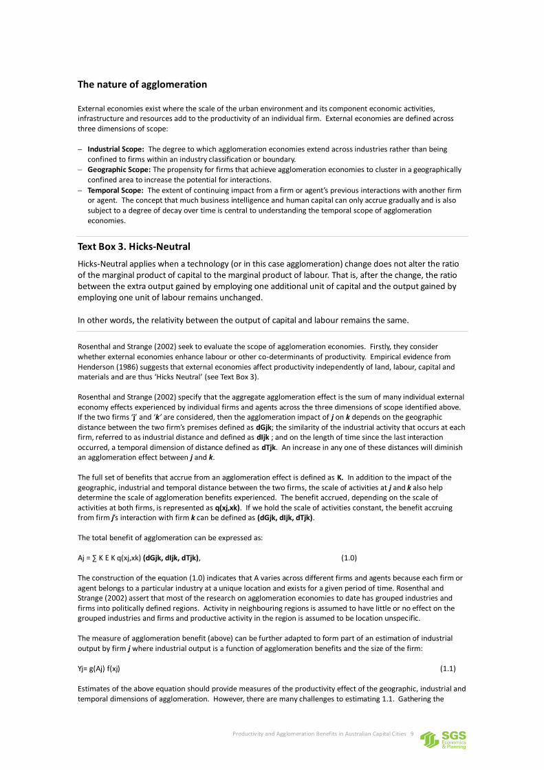
External economies exist where the scale of the urban environment and its component economic activities, infrastructure and resources add to the productivity of an individual firm. External economies are defined across three dimensions of scope:
Industrial Scope: The degree to which agglomeration economies extend across industries rather than being confined to firms within an industry classification or boundary.
Geographic Scope: The propensity for firms that achieve agglomeration economies to cluster in a geographically confined area to increase the potential for interactions.
Temporal Scope: The extent of continuing impact from a firm or agent’s previous interactions with another firm or agent. The concept that much business intelligence and human capital can only accrue gradually and is also subject to a degree of decay over time is central to understanding the temporal scope of agglomeration economies.
Text Box 3. Hicks-Neutral
Hicks-Neutral applies when a technology (or in this case agglomeration) change does not alter the ratio of the marginal product of capital to the marginal product of labour. That is, after the change, the ratio between the extra output gained by employing one additional unit of capital and the output gained by employing one unit of labour remains unchanged.
In other words, the relativity between the output of capital and labour remains the same.
Rosenthal and Strange (2002) seek to evaluate the scope of agglomeration economies. Firstly, they consider whether external economies enhance labour or other co-determinants of productivity. Empirical evidence from Henderson (1986) suggests that external economies affect productivity independently of land, labour, capital and materials and are thus ‘Hicks Neutral’ (see Text Box 3). Rosenthal and Strange (2002) specify that the aggregate agglomeration effect is the sum of many individual external economy effects experienced by individual firms and agents across the three dimensions of scope identified above. If the two firms ‘j’ and ‘k’ are considered, then the agglomeration impact of j on k depends on the geographic distance between the two firm’s premises defined as dGjk; the similarity of the industrial activity that occurs at each firm, referred to as industrial distance and defined as dIjk ; and on the length of time since the last interaction occurred, a temporal dimension of distance defined as dTjk. An increase in any one of these distances will diminish an agglomeration effect between j and k. The full set of benefits that accrue from an agglomeration effect is defined as K. In addition to the impact of the geographic, industrial and temporal distance between the two firms, the scale of activities at j and k also help determine the scale of agglomeration benefits experienced. The benefit accrued, depending on the scale of activities at both firms, is represented as q(xj,xk). If we hold the scale of activities constant, the benefit accruing from firm j’s interaction with firm k can be defined as (dGjk, dIjk, dTjk). The total benefit of agglomeration can be expressed as: Aj = ∑ K E K q(xj,xk) (dGjk, dIjk, dTjk), (1.0) The construction of the equation (1.0) indicates that A varies across different firms and agents because each firm or agent belongs to a particular industry at a unique location and exists for a given period of time. Rosenthal and Strange (2002) assert that most of the research on agglomeration economies to date has grouped industries and firms into politically defined regions. Activity in neighbouring regions is assumed to have little or no effect on the grouped industries and firms and productive activity in the region is assumed to be location unspecific. The measure of agglomeration benefit (above) can be further adapted to form part of an estimation of industrial output by firm j where industrial output is a function of agglomeration benefits and the size of the firm: Yj= g(Aj) f(xj) (1.1) Estimates of the above equation should provide measures of the productivity effect of the geographic, industrial and temporal dimensions of agglomeration. However, there are many challenges to estimating 1.1. Gathering the

Productivity and Agglomeration Benefits in Australian Capital Cities 10
information required to resolve all three dimensions of agglomeration benefits presents a daunting exercise and would involve measuring all forms of economic activity by industry and distance from j across a wide history of interaction. Thus, most agglomeration models only consider one or two of the three dimensions of agglomeration scope. In estimating (1.1), measures of labour, material and land inputs into a firm’s production process can be made from public data sets (especially in the case of labour but also for material). Measures of land use and other production inputs (such as capital) are generally more difficult to obtain. Where data is made available to the researcher at the level of an individual plant within a firm, more accurate estimates of external economies of scale are possible, such as those made by Henderson (2003b). Measurement error is another central challenge in estimating productivity effects. This has been surveyed considerably by Eberts and McMillen (1999). In larger cities, firms use capital and land more intensively than in smaller cities and this can create bias in the coefficient estimates when taken for firms operating in cities of different sizes (Moomaw 1981). In response to the challenges presented when trying to estimate the production function of a firm or plant, four indirect means of investigating the scope of agglomeration economies have been developed in the literature.
1. Study the growth in total employment resulting from agglomeration across a region or local area.
2. Identify new firms or plant start-ups and the number of jobs created.
3. Study the change in wages resulting from agglomeration across a region or local area.
4. Study the change in rents resulting from agglomeration across a region or local area.
There continues to be debate as to whether agglomeration economies can be ascribed to the benefits from localisation or urbanisation economies. Recent contributions to the literature (World Bank 2009, as described earlier) have suggested that these are separable and often concurrent sources of productivity advantage. Localisation economies resonate with the concept of industry clusters and are more relevant to smaller cities and towns (for example, European and Chinese cities specialising in particular manufacturing products). The concept of industry clusters relates to firms co-locating due to links within the production chain. Firms get a significant benefit from the depth of skills available for a particular sector. Urbanisation economies, on the other hand, require much larger cities and flow from the ‘cross-fertilisation’ of ideas between sectors. In this sense, agglomeration also plays out through the co-location of firms, yet these firms are not necessarily linked via a production chain. Clearly, the increased density of economic activity brought about by transport and land use projects could drive both the localisation and urbanisation components of agglomeration, but are more likely to be influential with the latter depending on the scale of the city in question.
The macroeconomic underpinnings of agglomeration
As mentioned earlier, the body of research on the macroeconomic underpinnings of agglomeration is not nearly as well developed as the microeconomic-based literature. In their working paper, Varga and Schalk (2004) attempt to converge areas of macroeconomic theory to develop a framework for empirically demonstrating how geographic structure, that is, localisation, can influence macroeconomic growth. These areas of macroeconomic theory are endogenous growth theory, the geography of knowledge spillovers, and new economic geography (Varga and Schalk 2004). This section examines literature which builds a link between agglomeration economies and endogenous growth theory, and more recently, with new economic geography theory.
Endogenous growth theory The premise of endogenous growth theory is that for productivity per capita to continue to grow over the long run, continual improvements to technology are required (Aghion and Howitt 1998). This is supported by neoclassical growth models demonstrating that without technological improvements or population growth, diminishing returns would be evident (Solow 1956, Swan 1956). In their work on endogenous growth theory, Aghion and Howitt (1998) demonstrate that population growth, in the absence of technological improvements, would also lead to a decline in aggregate output over time. Indeed, exogenous technological change is shown to be the only way long-run growth in output per capita may occur, so long as the change continually offsets the effect of diminishing returns (Aghion and Howitt 1998). Hinting at links to the notion of agglomeration economies, Aghion and Howitt (1998, p.34) note that researchers suggest factors which can be accumulated, such as ‘human capital, public infrastructure and possibly knowledge’, need to be better accounted for in endogenous growth models.

Productivity and Agglomeration Benefits in Australian Capital Cities 11
Romer (1986) shows that increased specialisation of labour across a widening pool of activities can lead to increasing returns over time. His thesis is that as an economy grows, a larger market offsets the fixed costs associated with producing a larger number of intermediate inputs. This in turn increases productivity of labour and capital, leading to growth. Endogenous growth theory helps to explain how increasing returns may be achieved via specialisation and knowledge and innovation, yet it does not account for spatial organisation and how this can contribute to productivity. New economic geography helps to bridge this gap.
New economic geography The field of spatial economics is not as well-established as other aspects of economic theory and empirical research. Krugman (1998) defines spatial economic structure as a result of the ‘interplay between two opposite forces’: centripetal forces which can lead to spatial concentration and centrifugal forces which lead to dispersed economic activity. Table 2 summarises these forces.
TAB L E 2 . FO R CES AFFECTI NG G EO G R A PH I CAL CO NCENTR ATI O N
Centripetal forces Centrifugal forces
Market-size effects (linkages) Immobile factors
Thick labour markets Land rents
Pure external economies Pure external diseconomies
Source: Krugman 1998, p.8
Krugman (1998) suggests that agglomeration economies are encouraged by urbanisation forces, a skilled, deep pool of labour and external economies. At the same time, factors which work against agglomeration include immobile factors, for example, proximity to fixed infrastructure such as a port, and land rents which can be higher in areas of greater economic density. There are certain diseconomies relating to agglomeration, evidenced by some producers operating and indeed thriving in peripheral locations. This relates to the centrifugal forces described by Krugman (1998). Negative externalities such as traffic congestion and high rents can reduce returns to scale in dense economies. If, however, transport costs increase with distance, firms will cluster to generate increasing returns. The idea of cities as ‘incubators’ of new firms and new ideas is linked to these forces. Several studies have supported the idea of new products more easily being developed in large, diverse metropolitan locations. In these locations, access to a wide pool of labour and services can help to establish new firms. However, mature products can survive in decentralised locations. Importantly, Krugman (1998) notes that spatial concentration of research and knowledge can promote spillovers. Varga (2000, 2001) provides empirical evidence which suggests spillover impact in knowledge production is correlated to the size of a region. Romer (1990) endogenises knowledge spillovers in his theory so as to account for geography in the growth model. More recent work by Rossi-Hansberg and Wright (2007) integrates a traditional microeconomic model of cities into an aggregate growth framework. Tension between ‘local increasing returns implied by the existence of cities, and aggregate constant returns, implied by balanced growth’ is addressed through a general equilibrium theory of economic growth in an urban environment (Rossi-Hansberg and Wright 2007, p.597).
The authors describe how the size of cities is endogenously influenced through agglomeration effects, which encourage growth, and congestion costs which encourage dispersal, and that the efficient organisation of cities can help to explain differences in total factor productivity across countries. Rossi-Hansberg and Wright (2007) highlight that efficient organisation of cities and the ability of government to apply effective spatial policy is an important determinant of income levels. Endogenous regional growth models are similar to new economic geography models. However, critiques have emerged from evolutionary economics researchers which suggest that many studies into macroeconomic explanations of agglomeration, whilst being mathematically complex, can be too simple, philosophically. Research into the links between macroeconomic theory and agglomeration economies is not as well-established as in microeconomic thought. However, evidence points to a complex relationship between aggregate output, knowledge spillovers and localisation economies.

Productivity and Agglomeration Benefits in Australian Capital Cities 12
The sources of agglomeration economies
Agglomeration arises both from the benefits of firms locating in an area where they can exploit a natural advantage and from firms locating together to take advantage of agglomeration economies. The relative contribution of each of these factors has been explored by Kim (1995, 1999) and Ellison and Glaeser (1999). Kim looked at agglomeration between 1860 and 1987 and regressed a location quotient – measuring the concentration of industry - against plant size, natural resource availability and dummy variables for industry sector and time. The positive coefficient returned for the natural resources variable suggested that this was highly significant. Ellison and Glaeser showed that 20 percent of agglomeration can be predicted by the presence of natural advantages. However, it is likely that, over time, the role of natural advantage in determining agglomeration has been decreasing because labour has become more mobile – enabling industries to concentrate in an area and enjoy agglomeration economies by importing labour. The research reveals little about the micro foundations of agglomeration economies. Agglomeration economies typically involve knowledge sharing, labour pooling and input sharing. Any one or multiple combinations of these micro foundations can increase productivity, which increases profitability, and leads to firm growth (Helsey and Strange, 2001). Glaeser and Mare (2001) propose that by looking at the dynamic structure of agglomeration economies, the separate contributions of different micro foundations can be identified. The lag in wage increases in response to urbanisation suggests that these shifts are the result of knowledge spillovers. Alternatively, Henderson (2003a) suggests that looking at the impact of the number of firms in a location on the productivity of their neighbours will capture the impact of knowledge spillovers. This sub-section introduces sources of agglomeration, while the following sub-section provides evidence of these sources in further detail.
Input sharing The concept of input sharing depends on the existence of scale economies in purchasing production inputs (Marshall, 1920). Without scale economies, an isolated firm could request a small batch of a production input and pay the same per unit price as for a larger order from a collective of firms. In instances where producers receive collective or multiple demands for an input, they can achieve the cost advantages from an efficient scale of production and pass some of this gain on to their customers.
Knowledge and technological spillovers With knowledge and technological spillovers, information is often exchanged between firms without being bought or sold – in contrast to input sharing (Helsey and Strange, 2002). Where exchanges do occur, these are likely to be compacted joint ventures for which data is not routinely collected. Romer (1990) defines two key sources of increasing returns: specialisation and knowledge spillovers. Economically useful knowledge is categorised into two aspects. The first is codified knowledge, which is knowledge published in books, scientific papers or patent documentation. Codified knowledge is non-rival yet partially excludable due to patenting. Nonetheless, such knowledge usually spills over into other areas. The second aspect is tacit knowledge.
Labour market pooling There are two related explanations for labour market pooling. One is that workers in large cities or industrial concentrations should be better matched to their roles. This can be examined by looking at termination rates, controlling for conditions in the local economy and industry sector. However, because employers of firms in smaller cities have fewer options with which to replace an employee should they decide to terminate the employment of that person, the actual termination rates might not indicate the full extent of matching unsuitability. Alternatively, rates of employee turnover could be studied to identify labour market pooling; high employee turnover rates indicate that workers can readily change jobs and firms can readily hire new employees. Baumgartner (1988) looks at medical practitioners and shows that in larger markets, practitioners perform a narrower range of activities, confirming that agglomeration can foster specialisation. The other explanation for labour market pooling is that it is based on risk. When a new employee commences with a firm, both the employee and the firm suffer costs if the relationship is unsuccessful and the employee is terminated. The worker will need to find another job and the employer will need to find another employee. Where the worker’s skills and the firm’s requirements are specific to an industry, both of these needs are more easily met where the industry is concentrated and there are alternative firms and alternative potential employees. Worker and firm risk are both reduced by localisation. However, industries are subject to periodic ‘shocks’ that result in workers losing their jobs. Locating in a specialised city exposes workers to a potentially greater risk of losing their job and being unable to find alternative employment locally. While this finding is intuitively sound it is difficult to test in an
Productivity and Agglomeration Benefits in Australian Capital Cities 13
Australian environment. Australia’s limited number of major cities means that there is not the level of city specialisation which is observed in the United States or Europe.
The home market effect Suppose that increasing returns result in the concentration of employment into a large factory. This, in turn, creates a large market for suppliers who seek to locate close to the large factory to reduce their transport costs. This leads to a ‘magnification’ effect where the ‘home market’ (the large factory and its suppliers) expand in a self-reinforcing process of agglomeration.
Consumption While it is broadly accepted that cities contribute to industry agglomeration and industry productivity, recent research also looks at the role of the demand side in large cities in encouraging consumption driven agglomeration of city firms. Glaeser (2001) argues that there are four processes by which this can happen. Firstly, the population of the city is large enough to create a viable local market for some goods and services that are not available in smaller centres (such as operatic performances). Secondly, a large city may create an aesthetic charm (‘pace’, ‘style’ or ‘mood’) which enhances citizen and visitor sense of wellbeing and, in doing so, encourages citizens and visitors to spend more money on leisure, food and beverage and retail goods. Thirdly, the population of the city is large enough for the provision of public goods and services that are not available in smaller centres (such as specialised medical services). Fourthly, the dense settlement pattern of cities allows goods and information to be exchanged rapidly.
Agglomeration and human capital
Agglomeration also helps to improve the quality of labour inputs available by increasing the stock of human capital. OECD describes human capital as productive wealth embodied in labour, skills and knowledge. If a large range of jobs is on offer, a worker can search through these opportunities and best match their skills to the available job, thus maximising their acquisition of skills and experience. Further to this, they have the opportunity to work in a number of different jobs and hence gain a range of experiences (which can be seen as on-the-job investment in their education) which will also translate into higher productivity. Urbanisation (the increasing relative share of cities) is also cited by Mincer (1995) as a contributing factor in the development of human capital in the United States. This helps to confirm the Matching Theory explanation for higher human capital development. Matching theory relates to the creation of relationships which are mutually beneficial over time. Glaeser and Resseger (2010) present two core knowledge-based theories on urban agglomeration. The first is based on the Marshallian concept of density and how it can facilitate learning between workers. The second theory is based on high levels of human capital and city size having a cumulative effect in further increasing productivity and knowledge. Both of these ideas suggest that age-earning profiles could be steeper in larger, more skilled cities. However, for this to be the case, productivity gains from human capital must be higher than productivity gains via technological improvements. Glaeser and Resseger (2010) provide evidence that workers learn more quickly in large metropolitan areas, particularly in areas with a higher skills profile. Whilst urbanisation and localisation boost productivity via increased economies of scale and scope, human capital improvements also lead to productivity gains via improved job-matching.
Productivity and Agglomeration Benefits in Australian Capital Cities 14
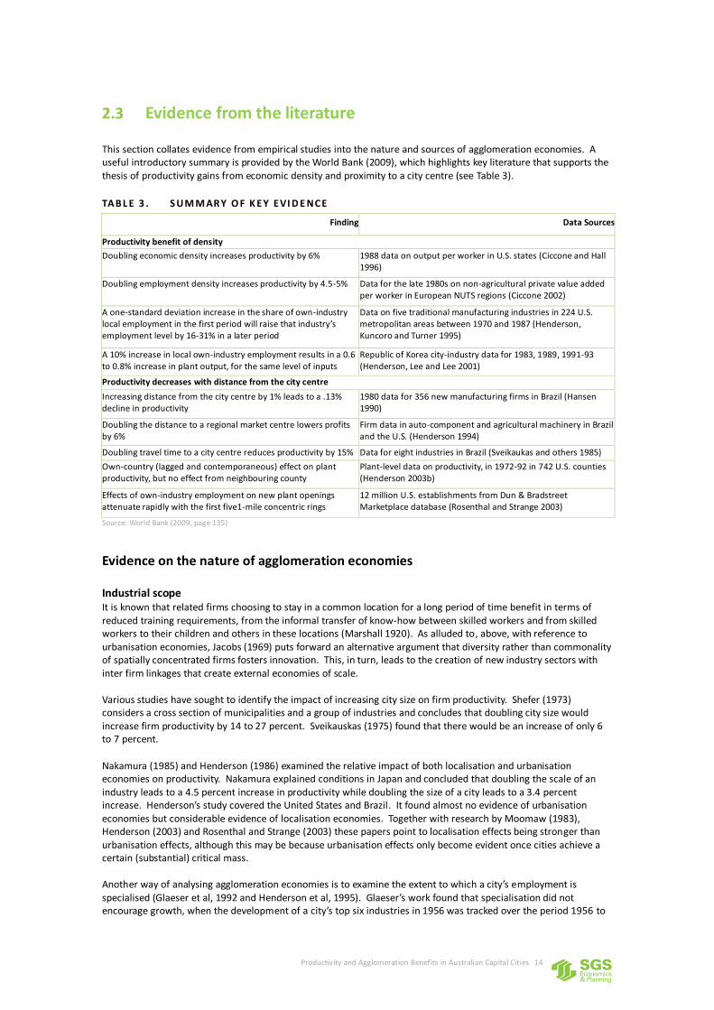
2.3 Evidence from the literature
This section collates evidence from empirical studies into the nature and sources of agglomeration economies. A useful introductory summary is provided by the World Bank (2009), which highlights key literature that supports the thesis of productivity gains from economic density and proximity to a city centre (see Table 3).
TAB L E 3 . S UM M AR Y O F K EY EVI D E NCE
Finding Data Sources
Productivity benefit of density
Doubling economic density increases productivity by 6% 1988 data on output per worker in U.S. states (Ciccone and Hall 1996)
Doubling employment density increases productivity by 4.5-5% Data for the late 1980s on non-agricultural private value added per worker in European NUTS regions (Ciccone 2002)
A one-standard deviation increase in the share of own-industry local employment in the first period will raise that industry’s employment level by 16-31% in a later period
Data on five traditional manufacturing industries in 224 U.S. metropolitan areas between 1970 and 1987 (Henderson, Kuncoro and Turner 1995)
A 10% increase in local own-industry employment results in a 0.6 to 0.8% increase in plant output, for the same level of inputs
Republic of Korea city-industry data for 1983, 1989, 1991-93 (Henderson, Lee and Lee 2001)
Productivity decreases with distance from the city centre
Increasing distance from the city centre by 1% leads to a .13% decline in productivity
1980 data for 356 new manufacturing firms in Brazil (Hansen 1990)
Doubling the distance to a regional market centre lowers profits by 6%
Firm data in auto-component and agricultural machinery in Brazil and the U.S. (Henderson 1994)
Doubling travel time to a city centre reduces productivity by 15% Data for eight industries in Brazil (Sveikaukas and others 1985)
Own-country (lagged and contemporaneous) effect on plant productivity, but no effect from neighbouring county
Plant-level data on productivity, in 1972-92 in 742 U.S. counties (Henderson 2003b)
Effects of own-industry employment on new plant openings attenuate rapidly with the first five1-mile concentric rings
12 million U.S. establishments from Dun & Bradstreet Marketplace database (Rosenthal and Strange 2003)
Source: World Bank (2009, page 135)
Evidence on the nature of agglomeration economies
Industrial scope It is known that related firms choosing to stay in a common location for a long period of time benefit in terms of reduced training requirements, from the informal transfer of know-how between skilled workers and from skilled workers to their children and others in these locations (Marshall 1920). As alluded to, above, with reference to urbanisation economies, Jacobs (1969) puts forward an alternative argument that diversity rather than commonality of spatially concentrated firms fosters innovation. This, in turn, leads to the creation of new industry sectors with inter firm linkages that create external economies of scale. Various studies have sought to identify the impact of increasing city size on firm productivity. Shefer (1973) considers a cross section of municipalities and a group of industries and concludes that doubling city size would increase firm productivity by 14 to 27 percent. Sveikauskas (1975) found that there would be an increase of only 6 to 7 percent. Nakamura (1985) and Henderson (1986) examined the relative impact of both localisation and urbanisation economies on productivity. Nakamura explained conditions in Japan and concluded that doubling the scale of an industry leads to a 4.5 percent increase in productivity while doubling the size of a city leads to a 3.4 percent increase. Henderson’s study covered the United States and Brazil. It found almost no evidence of urbanisation economies but considerable evidence of localisation economies. Together with research by Moomaw (1983), Henderson (2003) and Rosenthal and Strange (2003) these papers point to localisation effects being stronger than urbanisation effects, although this may be because urbanisation effects only become evident once cities achieve a certain (substantial) critical mass. Another way of analysing agglomeration economies is to examine the extent to which a city’s employment is specialised (Glaeser et al, 1992 and Henderson et al, 1995). Glaeser’s work found that specialisation did not encourage growth, when the development of a city’s top six industries in 1956 was tracked over the period 1956 to
Productivity and Agglomeration Benefits in Australian Capital Cities 15
1987. Henderson investigated eight different industries (three evolving as high tech and five as mature industries) from 1970 to 1987 and concluded that specialisation has a positive influence on growth for mature industries but that evolving industries perform better in cities with diverse industry profiles. Duranton and Puga (2003) use French data to show that as some industries reach maturity they move from diverse cities to those with a less varied industrial profile. Theories on the origin of agglomeration economies have almost always been grounded in the concept that increasing the absolute scale of an industrial activity invariably brings benefits. For example, having more workers to choose from means workers are employed in jobs better suited to their skills (Helsey and Strange, 1990). The flip side to this argument is that diversity of industries brings cross fertilisation of technologies and leads to the birth of new industries and growth and innovation in existing ones (Chinitz, 1961). Combes (2000) finds that specialisation and diversity both have negative effects on growth for all but a few industry sectors within manufacturing. But when the same analysis is made for service industries, Combes found that while specialisation continued to have a negative effect on growth, diversity had a positive effect. The question of how agglomeration economies subside as nearby activity becomes increasingly dissimilar remains little explored in the literature. It is difficult to measure ‘industrial distance’, that is, the distance between the function of two industries. Cluster mapping based on supply relationships and the similarity of production processes such as by Ellison and Glaeser (1997) is the closest approximation available.
Geographic scope Until recently, research into agglomeration economies has defined geography on the basis of political boundaries and not assumed the gradation of effects within, and in response to firms from outside, these boundaries. Ciccone and Hall (1996) departed from this approach and measured employment density across New York State at the local (county) level. They found that doubling county population density led to an approximately 5 percent increase in productivity. Dekle and Eaton (1999) used rents to identify agglomeration economies for finance and manufacturing in Japanese prefectures. The results suggested a weak relationship to increasing urban size – a 1 percent increase in productivity for a doubling of population. Rosenthal and Strange (2003) found that industries which relied more heavily on manufactured or natural products inputs, or which produced perishable products, were more inclined to concentrate in geographic proximity. Ellison and Glaeser (1997) and Duranton and Overmans (2002) measured industry concentration and agglomeration effects at different scales and concluded that the effects are localised. Duranton and Overman (2002) found that localisation benefits dissipate beyond 50 kilometres of distance. With reference to the UK, Graham (2006) found a productivity elasticity of 0.1251 for the whole economy, 0.052 for manufacturing (with large variation within the industry) and 0.20 for services. Broadly speaking, this aligns with the theory that services prosper in very large and well-connected cities because of the rich pool of ideas on offer, whereas sectors with relatively fixed or mature business models – like manufacturing – do better in clustered locations which are relatively free of urban congestion and high land costs (World Bank, 2009). The European Conference of Transport Minister’s Round Table (2001) outlines that, by widening the area of goods markets, transport improvements may promote competition, thereby enhancing economic efficiency. The effect may be analogous to the removal of customs barriers. The removal of such barriers results in higher productivity and raises the purchasing power of populations, which benefit from the specialisation of trade. Secondly, improved transport links which increase travel speeds may have the same effect as increasing the size of the employment market, as a greater number of job-seekers will be able to travel to more distant jobs. This will allow for greater productivity as employers are better able to find employees qualified for the jobs they are seeking to fill. The Commonwealth Treasury2 outlines that “The Government also has a role in investing directly in infrastructure, innovation and Human Capital. Such direct investment may be necessary where markets for a good or service are incomplete, goods have public good characteristics, or there are positive spillovers associated with the production of a good or service”. While the Treasury recognised that there are “spillovers” which come from infrastructure and human capital investments, a methodological framework to measure the benefits from these investments is not provided.
1 That is, a doubling of job density leads to a 12.5% increase in the productivity of firms. 2 www.treasury.gov.au/.../4_Productivity_Growth_Submission.rtf

Productivity and Agglomeration Benefits in Australian Capital Cities 16
Temporal scope A key issue in the literature about agglomeration economies is the question as to whether past economic environments (say, from previous decades) can continue to impact agglomeration economies many years later, albeit indirectly. Glaeser et al (1992) and Henderson et al (1995) both incorporate this consideration into their growth models. A direct dynamic effect (often referred to as ‘knowledge spill over’) involves industrial activity from many years ago positively influencing today’s productivity. A paper by Glaeser and Mare (2001) estimates the temporal scope of agglomeration economies by regressing data on wage rates against a range of worker and location attributes. This analysis shows that there is an urban wage premium of approximately 20 percent but that this premium is enjoyed more by long time city residents than by recent immigrants. Also, when long time urban workers leave their city, the wages they earn in their new location are higher the larger the city they move from. This reflects the portability of the human capital development benefits offered by urbanisation.
Human capital and its links to agglomeration
Glaeser and Resseger (2010) note that there is a strong correlation between per-worker productivity and metropolitan area population in cities with high skill levels, but that this does not hold for less skilled metropolitan areas in the United States. The authors note that area population (urbanisation) can explain 45 percent of the variation in per-worker productivity. Over the past 50 years
3 the concept of human capital has been at the forefront of economic theory and practice.
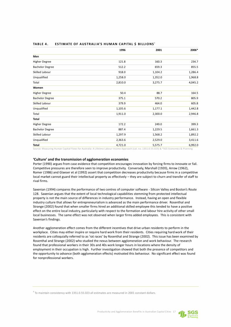
Human capital comprises the knowledge and skills which enable a worker to contribute to a firm’s production and to earn a wage. Human capital can be expanded by investment (formal education and experience gained by workers) which will increase the worker’s skill, and hence productivity. Human capital theory can be used in seeking to understand labour market outcomes and the distribution of income across society. Moreover, it also key to understanding growth in GDP. The ABS has measured Human Capital in Australia for 1981-2001 and published the estimates in Measuring Human Capital Flows for Australia: A Lifetime Labour Income Approach (cat. no. 1351.0.55.023 – see Table 4.
3 Since Becker & Schultz published their seminal work in the 1960’s.
Productivity and Agglomeration Benefits in Australian Capital Cities 17
TAB L E 4 . ES TIM ATE O F AUS TR AL I A’S H UM AN CAPI TAL $ BI LLI O NS 4
1996 2001 2006*
Men
Higher Degree 121.8 160.3 234.7
Bachelor Degree 512.2 659.3 855.5
Skilled Labour 918.0 1,104.2 1,286.4
Unqualified 1,258.0 1,352.0 1,968.8
Total 2,810.0 3,275.7 4,045.2
Women
Higher Degree 50.4 88.7 164.5
Bachelor Degree 375.1 570.2 805.9
Skilled Labour 379.9 464.0 605.8
Unqualified 1,105.6 1,177.1 1,442.8
Total 1,911.0 2,300.0 2,946.8
Total
Higher Degree 172.2 249.0 399.3
Bachelor Degree 887.4 1,229.5 1,661.3
Skilled Labour 1,297.9 1,568.2 1,892.2
Unqualified 2,363.6 2,529.0 3,411.6
Total 4,721.0 5,575.7 6,992.0 Source: Measuring Human Capital Flows for Australia: A Lifetime Labour Income Approach (cat. no. 1351.0.55.023) & *SGS Economics & Planning
‘Culture’ and the transmission of agglomeration economies Porter (1990) argues from case evidence that competition encourages innovation by forcing firms to innovate or fail. Competitive pressures are therefore seen to improve productivity. Conversely, Marshall (1920), Arrow (1962), Romer (1986) and Glaeser et al (1992) assert that competition decreases productivity because firms in a competitive local market cannot guard their intellectual property as effectively – they are subject to churn and transfer of staff to rival firms. Saxenian (1994) compares the performance of two centres of computer software - Silicon Valley and Boston’s Route 128. Saxenian argues that the extent of local technological capabilities stemming from protected intellectual property is not the main source of differences in industry performance. Instead, having an open and flexible industry culture that allows for entrepreneurialism is advanced as the main performance driver. Rosenthal and Strange (2002) found that when smaller firms hired an additional skilled employee this tended to have a positive effect on the entire local industry, particularly with respect to the formation and labour hire activity of other small local businesses. The same effect was not observed when larger firms added employees. This is consistent with Saxenian’s findings. Another agglomeration effect comes from the different incentives that drive urban residents to perform in the workplace. Cities may either inspire or require hard work from their residents. Cities requiring hard work of their residents are colloquially referred to as ‘rat races’ by Rosenthal and Strange (2002). This issue has been examined by Rosenthal and Strange (2002) who studied the nexus between agglomeration and work behaviour. The research found that professional workers in their 30s and 40s work longer hours in locations where the density of employment in their occupation is high. Further investigation showed that both the presence of competitors and the opportunity to advance (both agglomeration effects) motivated this behaviour. No significant effect was found for nonprofessional workers.
4 To maintain consistency with 1351.0.55.023 all estimates are measured in 2001 constant dollars.
Productivity and Agglomeration Benefits in Australian Capital Cities 18
Evidence of sources of agglomeration economies
Evidence of input sharing Holmes (1999) investigates the connection between a firm’s location in close concentration with similar firms and its engagement in input sharing with other firms. Holmes uses Census data on manufacturing sales at the establishment (firm) level and Census data on purchased inputs. Purchased inputs are divided by sales to give purchased input intensity which is also a measure of vertical dis-integration or input sharing. The differences in purchased input intensity between locations of concentrated similar firms and other locations across the USA were then examined. It was found that across all industries, moving from an un-concentrated location (fewer than 500 employees in the same industry) to a concentrated location (10,000 to 24,999 neighbouring employees in the same industry) resulted in a 3 percent increase in purchased input intensity. It can also be expected that in the presence of input sharing by purchasers, input suppliers would carry out more specialised functions. Because industry classification protocols typically place vertically integrated stages of production in the same category, it is difficult to test this theory. Holmes looks at the textile industry for which specialised textile finishing plants are afforded a separate industry classification from the rest of the industry, finding that where the industry was more concentrated, the ratio of specialised finishing plants to total plants tended to be higher. World Bank (2009) suggests input-sharing is an important channel for agglomeration economies, as density of activity allows more refined specialisation and wider variety of intermediate inputs.
Evidence of knowledge and technological spillovers To address the challenges of a lack of official data about knowledge spillovers, Jaffee et al (1993) use the location of firm patent citations to create a ‘paper trail’ of knowledge and technological spillovers. They found that spillovers from research to firms are greater when research and firms are co-located, with citations five to 10 times more likely to come from the same municipal area than control patents. This effect is expected to vary with industry scope – being most pronounced in those industries that are highly innovative or knowledge intensive (Audretsch and Feldman, 1996). Workers are the primary carriers of knowledge and technological spillovers. Rauch (1993) looks at the impact of education levels on wages and rents. Where average education levels were high in a district based sector this sharing of information as a public good was shown to increase wages across the sector. Rents were also shown to be higher, because the productivity reflected in higher wages was capitalised by the housing market. Charlot and Duranton (2002) find that workplace communication is more extensive in urban areas but that this accounts for only 10 percent of the urban education effect. This suggests that other knowledge and technological spillovers are taking place or that improved education levels impact other micro foundations of agglomeration economies. In summary, the exact channel of interaction whereby increased levels of education flows through to increase productivity across an industry sector is poorly understood.
Evidence of labour market pooling Simon (1988) considers the relationship between the unemployment rate and a city’s level of specialisation. Unemployment rates are shown to be greater in cities with higher degrees of specialisation - consistent with the idea of industry shocks being an important issue. It could therefore be expected that workers in specialised cities demand higher wages to compensate them for this risk. Diamond and Simon (1990) show that workers do, indeed, demand higher wages in more specialised cities and that these higher wages are also related to the cyclical variability of employment by industry. Costa and Kahn (2001) advance the argument that risk is lower and matches of employee to role are better in larger cities. In looking at ’power couples‘ – married couples where both partners have at least a bachelor degree qualification - Costa and Kahn documented a substantial increase over time in the proportional representation of this group in large cities – from 32 percent in 1940 to 50 percent in 1990. This may result from these couples having met, partnered and stayed in large cities, or it may be explained by large cities being better able to offer career opportunities that closely match the abilities of both partners than smaller cities. To test for each of these explanations, Costa and Kahn look at the differences between the location patterns of ’power couples‘ other types of couples, single persons and unmarried couples and concluded that 36 percent of the increase in concentration of ‘power couples‘ in large cities can be ascribed to the dual career hypothesis. Therefore, if the productivity of the highly educated is important for economic performance, large cities have a productivity advantage in so far as they have the ability to better match employees to roles that meet their abilities and achievable aspirations.
Productivity and Agglomeration Benefits in Australian Capital Cities 19
Evidence of the home market effect Krugman (1980) and Davis & Weinstein (1996) formally investigated this phenomenon, examining regional agglomeration across Japanese prefectures. They identified substantial increasing return effects on industrial concentration in eight of 19 prefectures. They concluded that the home market effect is an important determinant of regional concentration in both large cities and smaller localities. Hanson (1998a) looked at the shift in Mexican industrial production from Mexico City to cities along the US border in response to the NAFTA trade liberalisation agreement. In this instance, the opportunities from trade with international markets began to outweigh home market advantages from locating in the Mexico City megalopolis.
Consumption Taking Glaeser’s (2001) work as a base, Waldfogel (2003) investigates the concept that the larger markets in cities enable goods to be more closely tailored to individual consumer tastes. Waldfogel looked at radio listening patterns and identified that as a city’s population increased by one million residents, the proportion of the population who listened to radio increased by 2percent. Waldfogel identified that the number of radio stations targeting particular ethno linguistic subcultures (African and Hispanic) also increased with city population size. This suggested that radio stations were able to diversify their offer in larger cities and thus increase their total listening audience (market size). Tabuchi and Yoshida (2000) found that the real wages (spending power) of city residents was elastic (by between -7 and 12 percent) depending on city size. This is evidence that some city residents are willing to forego wages to enjoy the consumption benefits of living in a large city.
Macroeconomic implications of agglomeration
Davis, Fisher and Whited (2011) explore how important agglomeration is for aggregate growth via a dynamic stochastic general equilibrium model of cities, using aggregate data and city-level panel data. They find that local agglomeration has an impact on the growth rate of per capita consumption, raising it by about 10 percent. At the same time, this approach finds the net impact of density to be relatively small. Notably, the authors estimate that without agglomeration benefits, per capita consumption and housing would need to be ‘three percent large in each period in perpetuity’.
2.4 Conclusions
The literature offers considerable evidence that productivity is significantly affected by the size and structure of cities. The concepts of urbanisation and localisation are important here. In developing economies, greater investment in technology and human capital improvements (skills and education) may be prioritised in generating a greater mass of economic activity. In developed economies, where additional sources of competitive advantage must be secured, the question of localisation becomes paramount, with the way cities are structured and how they function being key to productivity enhancements. A city which is large but dysfunctional in a transport sense will not optimise its potential for agglomeration economies. ‘City shaping’ transport investments (such as major freeways, metros and commuter railway infrastructure) and interventions to create employment nodes in strategic locations are of vital significance in this context. For policy makers, this means that land use, transport and economic planning need to go hand-in-hand. Whilst the macroeconomic underpinnings of agglomeration are not as well-advanced as microeconomic explanations, the preliminary body of research highlights how urban policy and city-shaping infrastructure might contribute to aggregate total factor productivity (Rossi-Hansberg and Wright 2007, p.616).

Productivity and Agglomeration Benefits in Australian Capital Cities 20
3 PRACTICAL APPLICATION IN AUSTRALIAN PROJECT AND POLICY ASSESSMENT
3.1 Purpose
The purpose of this section is to provide practical guidance to project evaluators on how to assess the productivity and human capital effects of projects and planning policies that might affect economic agglomeration. It sets out a recommended methodology and identifies all relevant data sources required to operationalise this approach in any given city. To illustrate the method, three case studies are provided, two covering transport projects and one dealing with a land use planning initiative.
3.2 Overview of method – labour productivity and agglomeration
This sub-section introduces the overall method (see Figure 1 below) for estimating and applying productivity elasticities with respect to agglomeration. The latter is measured by effective job density (EJD). The EJD of an area is the sum employment in the area and the employment in all other areas divided by the travel time in reaching these external jobs, with travel time weighted for transport mode. The first stage in the method is to assemble the four data sets required in this process. These are a travel time matrix, employment and population at a small area level, labour productivity by sector at a state and city level, and then at a small area level. A travel time matrix shows how long it takes to travel from one small area in the city to all other small areas by car and public transport separately. This is produced within the transport modelling conducted externally to this process. Employment and population can be sourced from the Australian Bureau of Statistics (ABS) and other government departments and is required for the EJD calculation. Labour productivity is released by the ABS at the state level which can then be broken down into a city and balance of state estimate. This is done via the same method the ABS uses in its National Accounting Framework. The city level labour productivity is then broken down into a statistical local area (SLA) level using the same principles set out by the Australian System of National Accounts. The next stage is to calculate EJD at a small area level under a base case scenario. The two inputs are the travel time matrix and employment at a small area level. Once EJD has been calculated, a regression analysis using these estimates and labour productivity by sector can be conducted. This allows for the estimation of industry elasticities which show the impact on labour productivity of a doubling in EJD. The change in EJD brought about by a specific infrastructure or land use project can then be established in the same way the base case EJD is estimated. The inputs into this estimation will differ in terms of a changed travel time matrix or employment numbers. Finally the impact on gross value added (GVA) arising from changes to labour productivity can be quantified. This is completed via the use of the industry elasticities applied to the estimated changes to EJD to determine the changes to labour productivity. This altered labour productivity then flows through to a change in gross value added across industries and SLAs.
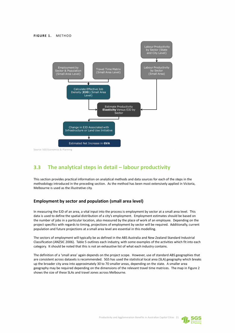
Productivity and Agglomeration Benefits in Australian Capital Cities 21
FI G UR E 1 . METH O D
Source: SGS Economics & Planning
3.3 The analytical steps in detail – labour productivity
This section provides practical information on analytical methods and data sources for each of the steps in the methodology introduced in the preceding section. As the method has been most extensively applied in Victoria, Melbourne is used as the illustrative city.
Employment by sector and population (small area level)
In measuring the EJD of an area, a vital input into the process is employment by sector at a small area level. This data is used to define the spatial distribution of a city’s employment. Employment estimates should be based on the number of jobs in a particular location, also measured by the place of work of an employee. Depending on the project specifics with regards to timing, projections of employment by sector will be required. Additionally, current population and future projections at a small area level are essential in this modelling. The sectors of employment will typically be as defined in the ABS Australia and New Zealand Standard Industrial Classification (ANZSIC 2006). Table 5 outlines each industry, with some examples of the activities which fit into each category. It should be noted that this is not an exhaustive list of what each industry contains. The definition of a ‘small area’ again depends on the project scope. However, use of standard ABS geographies that are consistent across datasets is recommended. SGS has used the statistical local area (SLA) geography which breaks up the broader city area into approximately 30 to 70 smaller areas, depending on the state. A smaller area geography may be required depending on the dimensions of the relevant travel time matrices. The map in Figure 2 shows the size of these SLAs and travel zones across Melbourne.
Employment by Sector & Population (Small Area Level)
Travel Time Matrix(Small Area Level)
Labour Productivity by Sector (State and City Level)
Labour Productivity by Sector
(Small Area)
Estimated Net Increase in GVA
Estimate Productivity Elasticity Versus EJD by
Sector
Change in EJD Associated withInfrastructure or Land Use Initiative
Calculate Effective Job Density (EJD) (Small Area
Level)

Productivity and Agglomeration Benefits in Australian Capital Cities 22
TAB L E 5 . SECTO R CL ASSIF ICATIO NS
Industry Contains
Agriculture, Forestry & Fishing Farming, Forestry, Fishing, Aquaculture
Mining Coal Mining, Gas Extraction, Mineral Mining, Exploration
Manufacturing Food Products, Textiles, Wood & Paper, Petroleum, Metal, Machinery & Furniture Manufacturing
Electricity, Gas, Water & Waste Services Supply of Electricity, Gas & Water, Waste Collection & Treatment
Construction Building, Heavy & Civil Engineering Construction & Services
Wholesale Trade Material, Machinery, Motor Vehicle & Grocery Products Wholesaling
Retail Trade Motor Vehicle, Fuel, Food & Other Retailing
Accommodation &Food Services Accommodation, Cafes, Restaurants
Transport, Postal & Warehousing Road, Rail, Water & Air Transport, Postage & Support Services
Information Media & Telecommunications Publishing, Broadcasting, Internet Services Providers, Motion Picture Recording & Libraries
Financial & Insurance Services Banking, Superannuation & Insurance, Auxiliary Finance
Rental, Hiring & Real Estate Services Rental & Hiring Services, Property Operators & Real Estate Agents
Professional, Scientific & Technical Services Scientific Research, Architects, Legal, Accounting, Management, Consulting, Veterinary & Computer Related Services
Administrative & Support Services Employment Services, Travel Agencies, Pest Control, Packaging Services
Public Administration & Safety Government Administration, Defence, Public Order & Regulatory Services
Education & Training School, Tertiary & Adult Education
Health Care & Social Assistance Hospitals, Medical Services, Allied Health, Residential Care & Child Services
Arts & Recreation Services Museum, Parks & Gardens Operations, Creative & Performing Arts, Sports & Physical Recreation, Gambling
Other Services Automotive & General Maintenance, Personal Care, Funeral & Religious Services, Interest Groups
Source: ABS ANZSIC 2006
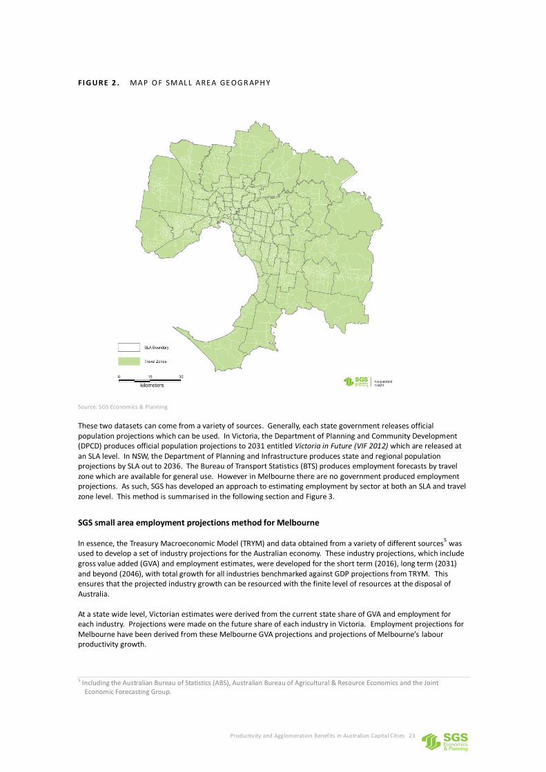
Productivity and Agglomeration Benefits in Australian Capital Cities 23
FI G UR E 2 . MAP O F SMAL L AREA GE OG R AP H Y
Source: SGS Economics & Planning
These two datasets can come from a variety of sources. Generally, each state government releases official population projections which can be used. In Victoria, the Department of Planning and Community Development (DPCD) produces official population projections to 2031 entitled Victoria in Future (VIF 2012) which are released at an SLA level. In NSW, the Department of Planning and Infrastructure produces state and regional population projections by SLA out to 2036. The Bureau of Transport Statistics (BTS) produces employment forecasts by travel zone which are available for general use. However in Melbourne there are no government produced employment projections. As such, SGS has developed an approach to estimating employment by sector at both an SLA and travel zone level. This method is summarised in the following section and Figure 3.
SGS small area employment projections method for Melbourne In essence, the Treasury Macroeconomic Model (TRYM) and data obtained from a variety of different sources
5 was
used to develop a set of industry projections for the Australian economy. These industry projections, which include gross value added (GVA) and employment estimates, were developed for the short term (2016), long term (2031) and beyond (2046), with total growth for all industries benchmarked against GDP projections from TRYM. This ensures that the projected industry growth can be resourced with the finite level of resources at the disposal of Australia. At a state wide level, Victorian estimates were derived from the current state share of GVA and employment for each industry. Projections were made on the future share of each industry in Victoria. Employment projections for Melbourne have been derived from these Melbourne GVA projections and projections of Melbourne’s labour productivity growth.
5 Including the Australian Bureau of Statistics (ABS), Australian Bureau of Agricultural & Resource Economics and the Joint
Economic Forecasting Group.

Productivity and Agglomeration Benefits in Australian Capital Cities 24
Employment growth was capped using future labour force constraints. The labour force was based on the 2011 Victoria in Future (VIF 2011) and projections for labour force participation for each five year age group. Labour force projections were made separately for men and women to account for observed differences in their participation by age profiles. The Intergenerational Report
6 was used as a guide to workforce participation amongst various age
groups into the future. A projection of unemployment was also made to ensure a coherent picture of the future labour force. This set of metropolitan projections was the cap under which the small area employment projections were limited. The ABS Census Journey to Work data has been used to estimate employment in each SLA for 1996, 2001, and 2006. However, due to undercounting in this dataset, the estimates for Melbourne were benchmarked to annual average employment estimates for each industry from the Labour Force Survey for each year. An adjustment has been made to the Labour Force Survey to account for people who live in regional Victoria but travel to Melbourne for work. For 2002, 2004, 2006, 2008 and 2010
7, data from the City of Melbourne Census of Land Use and Employment (CLUE)
was used to adjust the Census Journey to Work industry shares for the most recent years. These employment figures were also split into blue collar and white collar employment using Census Journey to Work and Labour Force Survey data. In projecting future industry employment by SLA the following process was followed:
Initially, the 2016 to 2046 projections for each SLA’s employment by industry were assumed to follow the
growth pattern observed in Melbourne industry share between 1996 and 2011.
In 2026 and 2046 adjustments were made to this industry to share account for known projects and fixed
policies affecting the development of Melbourne.
VIF population projections for each SLA were used to adjust the projections for population serving
industries. This was done by observing the trends in population to industry employment between 1996
and 2011.
A factor analysis of each of Melbourne’s SLA was utilised to appropriately cater for expected changes in
employment distribution over time. This factor analysis included an assessment of each SLA’s prospects
and capacity for growth, transport connections, resident workforce characteristics, employment lands
availability and government spatial policy considerations. Importantly, this factor analysis was undertaken
separately for each major industry, to ensure that the level of granularity appropriately reflected their
respective location drivers.
For the years between 2016 and 2026, the projections were interpolated. That is, the assumed spatial
changes at 2026 were progressively introduced.
For 2031, 2036 and 2041, the employment projections were extrapolated using the 2026 and 2046 SLA
industry employment shares.
6 Treasury, Australian Government, 2010 7 For 2010 only estimates for Docklands have been released.
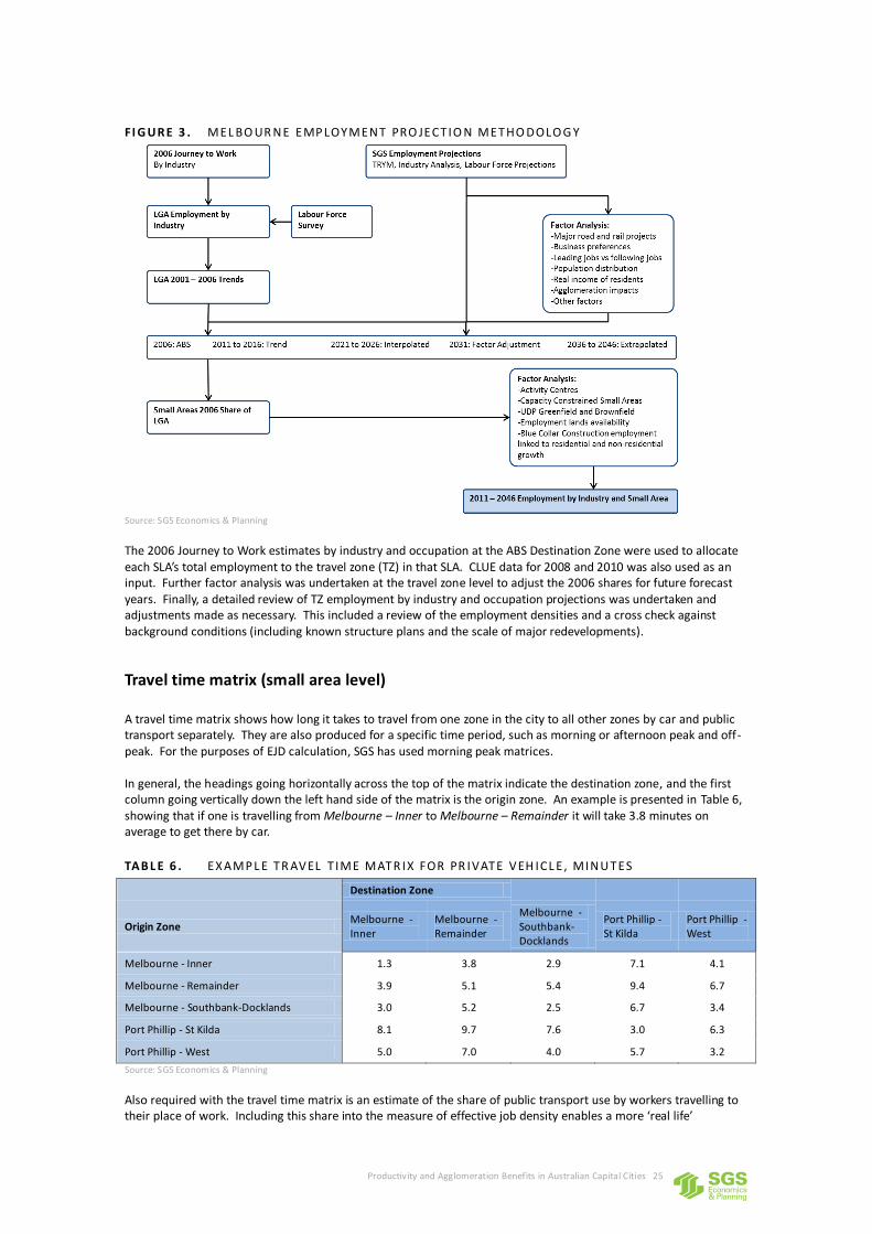
Productivity and Agglomeration Benefits in Australian Capital Cities 25
FI G UR E 3 . MEL BO UR NE EMP LOYMENT PRO JECT IO N METHO DOLO G Y
Source: SGS Economics & Planning
The 2006 Journey to Work estimates by industry and occupation at the ABS Destination Zone were used to allocate each SLA’s total employment to the travel zone (TZ) in that SLA. CLUE data for 2008 and 2010 was also used as an input. Further factor analysis was undertaken at the travel zone level to adjust the 2006 shares for future forecast years. Finally, a detailed review of TZ employment by industry and occupation projections was undertaken and adjustments made as necessary. This included a review of the employment densities and a cross check against background conditions (including known structure plans and the scale of major redevelopments).
Travel time matrix (small area level)
A travel time matrix shows how long it takes to travel from one zone in the city to all other zones by car and public transport separately. They are also produced for a specific time period, such as morning or afternoon peak and off-peak. For the purposes of EJD calculation, SGS has used morning peak matrices. In general, the headings going horizontally across the top of the matrix indicate the destination zone, and the first column going vertically down the left hand side of the matrix is the origin zone. An example is presented in Table 6, showing that if one is travelling from Melbourne – Inner to Melbourne – Remainder it will take 3.8 minutes on average to get there by car.
TAB L E 6 . EX AMP L E TR AVEL T IME MATR IX FOR PR IVATE VEH ICL E , MINU TES
Destination Zone
Origin Zone Melbourne - Inner
Melbourne - Remainder
Melbourne - Southbank-Docklands
Port Phillip - St Kilda
Port Phillip - West
Melbourne - Inner 1.3 3.8 2.9 7.1 4.1
Melbourne - Remainder 3.9 5.1 5.4 9.4 6.7
Melbourne - Southbank-Docklands 3.0 5.2 2.5 6.7 3.4
Port Phillip - St Kilda 8.1 9.7 7.6 3.0 6.3
Port Phillip - West 5.0 7.0 4.0 5.7 3.2
Source: SGS Economics & Planning
Also required with the travel time matrix is an estimate of the share of public transport use by workers travelling to their place of work. Including this share into the measure of effective job density enables a more ‘real life’
Productivity and Agglomeration Benefits in Australian Capital Cities 26
representation of the proximity (in terms of travel time) component of agglomeration. By way of illustration, 68 percent of people working in the CBD of Melbourne travel to work on public transport, implying that the proximity to those jobs is closely related to public transport travel times. The other extreme can be seen in locations such as Cranbourne (an outer suburb of Melbourne), where 98 percent of workers travel to work using private vehicles
8.
Throughout the estimation process, a small area has been defined as a statistical local area (SLA). However, as noted, a travel time matrix is generally produced at an even smaller geography due to the detailed nature of transport modelling. SGS has developed a methodology to convert these matrices from the travel zone level to an SLA level. This method could be applied to any travel time matrix given a concordance between the travel zones and SLAs. The steps involved in this method are outlined below, along with a simple worked example presented in Figure 4. Step 1: Convert the travel zone by travel zone travel time matrix (or generalised cost matrix) into a SLA by travel zone travel time matrix.
Step 2: Convert the SLA by travel zone travel time matrix into a SLA by SLA travel time (or generalised cost) matrix.
Where: = Travel Time from travel zone i to travel zone j
= Travel Time from SLA X to SLA Y = Population in Travel Zone i = Employment in Travel Zone j
It is possible the aggregation calculation from travel zone to SLA could be conducted in a number of ways. However, all methods should produce broadly the same result.
8 This method excludes travel times from other modes (bicycle or walk.)
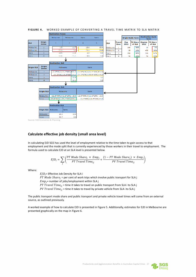
Productivity and Agglomeration Benefits in Australian Capital Cities 27
FI G UR E 4 . WOR K ED EX AMP L E O F CO NVER TING A TR AVEL T I ME MATR IX TO SL A MAT R IX
Source: SGS Economics & Planning
Calculate effective job density (small area level)
In calculating EJD SGS has used the level of employment relative to the time taken to gain access to that employment and the mode split that is currently experienced by those workers in their travel to employment. The formula used to calculate EJD at an SLA level is presented below.
Where:
= Effective Job Density for SLA i = per cent of work trips which involve public transport for SLA j
= number of jobs/employment within SLA j
= time it takes to travel on public transport from SLA i to SLA j
= time it takes to travel by private vehicle from SLA i to SLA j
The public transport mode share and public transport and private vehicle travel times will come from an external source, as outlined previously. A worked example of how to calculate EJD is presented in Figure 5. Additionally, estimates for EJD in Melbourne are presented graphically on the map in Figure 6.
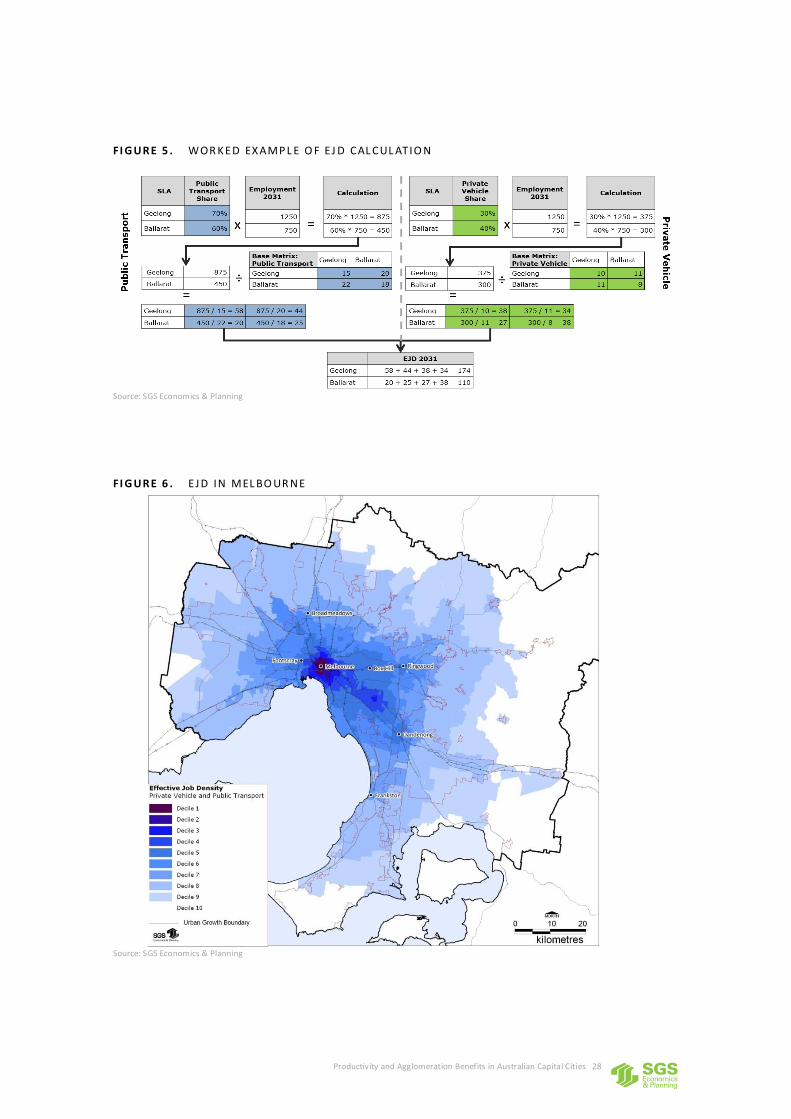
Productivity and Agglomeration Benefits in Australian Capital Cities 28
FI G UR E 5 . WOR K ED EX AMP L E O F EJ D CAL CUL ATIO N
Source: SGS Economics & Planning
FI G UR E 6 . EJ D IN MEL BO UR NE
Source: SGS Economics & Planning

Productivity and Agglomeration Benefits in Australian Capital Cities 29
Labour productivity by sector (state and capital city level)
Labour productivity is calculated by dividing the Gross Value Added (GVA) for an industry by the total number of hours worked in that industry.
Where: is the Labour Productivity for zone i is the Gross Value Added for zone i is the number of hours worked for zone i The estimate of GDP for each capital city is derived from industry data published in the Australian National Accounts: State Accounts (cat. no. 5220.0) publication. There are three approaches to measuring GDP; the Production approach (the sum of the GVA for each of the industries and taxes less subsides on products); the Expenditure approach (measures final expenditure on goods and services) and the Income approach (sum of income generated by all factors of production). At the Australian level, the Production, Expenditure and Income approaches are averaged by the ABS to produce GDP. However, at the state level, due to a lack of data on interstate trade, the Expenditure and Income approaches are combined and averaged with the Production approach. In developing the GDP
9 for each capital city the Production approach is used, firstly because of this lack of data on
intrastate trade. Another major reason is that the data available to calculate the Production approach is more robust (and hence requires fewer assumptions to be made) than that available for the Expenditure or Income approaches. For each industry, wherever possible, the same data sources which have been used to produce industry Gross Value Added at the state level are used to produce industry Gross Value Added at the city level. Some of these data sources include:
Agricultural Commodities: Small Area Data, Australia (cat. no. 7125.0)
Business Indicators, Australia (cat. no. 5676.0)
Manufacturing Industry, Australia (cat. no. 8221.0)
Regional Population Growth, Australia (cat. no. 3218.0)
Household Expenditure Survey (cat. no. 6530.0)
Education and Training Experience (cat. no. 6278.0)
Labour Force, Australia, Detailed, Quarterly (cat. no. 6291.0.55.003) In order to maintain consistency with the wider National Accounts, the Production approach estimate of Gross City Product is benchmarked to the Gross State Product using a statistical discrepancy method. Via the use of the implicit price deflation technique, the Chain Volume Measures of the Gross City Product are converted into Current Prices. This method overcomes the non-additivity issue with the Chain Volume Measure. The estimates of hours worked are derived from Information Paper: Implementing New Estimates of Hours Worked into the Australian National Accounts, 2006 (5204.0.55.003) which provides the total hours worked within the economy for 2004-05. The index of total hours worked from the Australian System of National Accounts, 2007-08 (cat. no. 5204.0) can be used to advance the 2004-05 estimate for the years between 2005-06 and 2007-08. This Australian ‘total hours worked’ figure can then been allocated for each industry in each capital city based on its share of total hours worked from the Labour Force, Australia, Detailed, Quarterly (cat. no. 6291.0.55.003). There are several advantages of using this measure of labour productivity. It is built on the National Accounts framework. This allows the agglomeration benefits to be viewed in the context of the wider economy. This includes the Australian, state and city economies. The National Accounts also provide a clear methodology for measuring economic activity and labour productivity. Direct comparisons of the benefits of agglomeration can be made between and within Australian cities. It should be noted that, in conducting this analysis, industries outside the Australian Bureau of Statistics Market Sector are included.
9 GDP (Gross Domestic Product) refers to Australia, GSP (Gross State Product) refers to a State, while GCP (Gross City Product)
refers to a city. But for simplicity’s sake in this paper all different measures are referred to as GDP.

Productivity and Agglomeration Benefits in Australian Capital Cities 30
As an example, Table 7 shows how the larger cities of Melbourne and Sydney have higher labour productivity than the smaller cities. This provides the first clear indication that the size of the economy of a city can provide improved outcomes for labour productivity. The industry mix within each city would also have an influence on the outcome. That is, more productive industries may tend to locate in particular cities.
TAB L E 7 . MAJ O R CAP ITAL C IT IES L ABO U R PRO DU CTIV ITY ( $ O F GRO SS VALU E AD DED P ER H OU R WO RK ED)
Sydney Melbourne Brisbane Adelaide Perth
1999 67.3 56.1 56.5 55.7 61.9
2004 71.2 61.9 61.3 59.5 71.6
2009 73.7 66.4 62.2 63.2 64.0
2011 75.7 66.3 64.0 64.5 71.1
Source: SGS Economics & Planning
Labour productivity by sector (small area level)
Unlike the UK, Australia does not currently offer readily accessible data sources on productivity at the level of the firm. This means that a synthetic dataset examining the issue needs to be created. Rather than attempting to focus on individual firms or workers the focus has been on creating robust estimates for defined geographical areas (SLAs). For Melbourne, the labour productivity estimates have been disaggregated by industry for each SLA, using the principles set out in the Australian System of National Accounts (ABS, 2000). Two separate methods were used for capital intensive industries (Manufacturing, Wholesale trade and Transport, postal and warehousing) and labour intensive industries (all other industries except for Electricity, gas, water and waste services and Information, media and telecommunications). For capital intensive industries, gross value added (GVA) per employee using the two digit Australia New Zealand Standard Industry Classification (ANZSIC 2006) level data sourced from Australian Industry, 2009-10 (cat. no. 8155.0) has been combined with detailed employment estimates for each SLA to calculate the GVA share of each SLA. This share has then been used to allocate the Melbourne total industry GVA to each SLA. For labour intensive industries a quality adjusted labour input method was used. That is, average industry wage rates were estimated for each SLA and combined with total hours worked for each industry for each SLA. This provides a proxy for total factor income for the SLA. This data on average industry wage rates and hours worked can be sourced from the ABS Census. The SLA share was then used to allocate the Melbourne total industry GVA to each SLA. Table 8 presents the labour productivity and EJD for a selection of Melbourne SLAs.
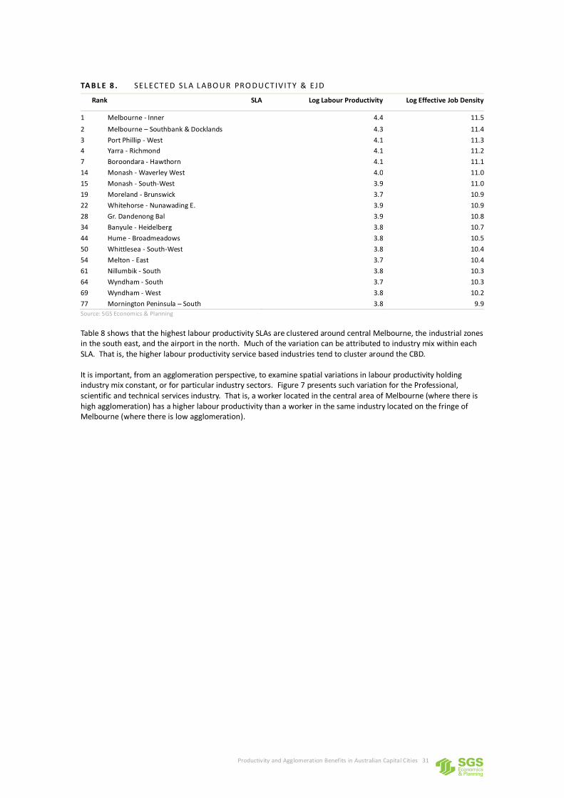
Productivity and Agglomeration Benefits in Australian Capital Cities 31
TAB L E 8 . SEL ECTED SL A L ABO U R PRO DU CTIV ITY & EJ D
Rank SLA Log Labour Productivity Log Effective Job Density
1 Melbourne - Inner 4.4 11.5
2 Melbourne – Southbank & Docklands 4.3 11.4
3 Port Phillip - West 4.1 11.3
4 Yarra - Richmond 4.1 11.2
7 Boroondara - Hawthorn 4.1 11.1
14 Monash - Waverley West 4.0 11.0
15 Monash - South-West 3.9 11.0
19 Moreland - Brunswick 3.7 10.9
22 Whitehorse - Nunawading E. 3.9 10.9
28 Gr. Dandenong Bal 3.9 10.8
34 Banyule - Heidelberg 3.8 10.7
44 Hume - Broadmeadows 3.8 10.5
50 Whittlesea - South-West 3.8 10.4
54 Melton - East 3.7 10.4
61 Nillumbik - South 3.8 10.3
64 Wyndham - South 3.7 10.3
69 Wyndham - West 3.8 10.2
77 Mornington Peninsula – South 3.8 9.9
Source: SGS Economics & Planning
Table 8 shows that the highest labour productivity SLAs are clustered around central Melbourne, the industrial zones in the south east, and the airport in the north. Much of the variation can be attributed to industry mix within each SLA. That is, the higher labour productivity service based industries tend to cluster around the CBD. It is important, from an agglomeration perspective, to examine spatial variations in labour productivity holding industry mix constant, or for particular industry sectors. Figure 7 presents such variation for the Professional, scientific and technical services industry. That is, a worker located in the central area of Melbourne (where there is high agglomeration) has a higher labour productivity than a worker in the same industry located on the fringe of Melbourne (where there is low agglomeration).
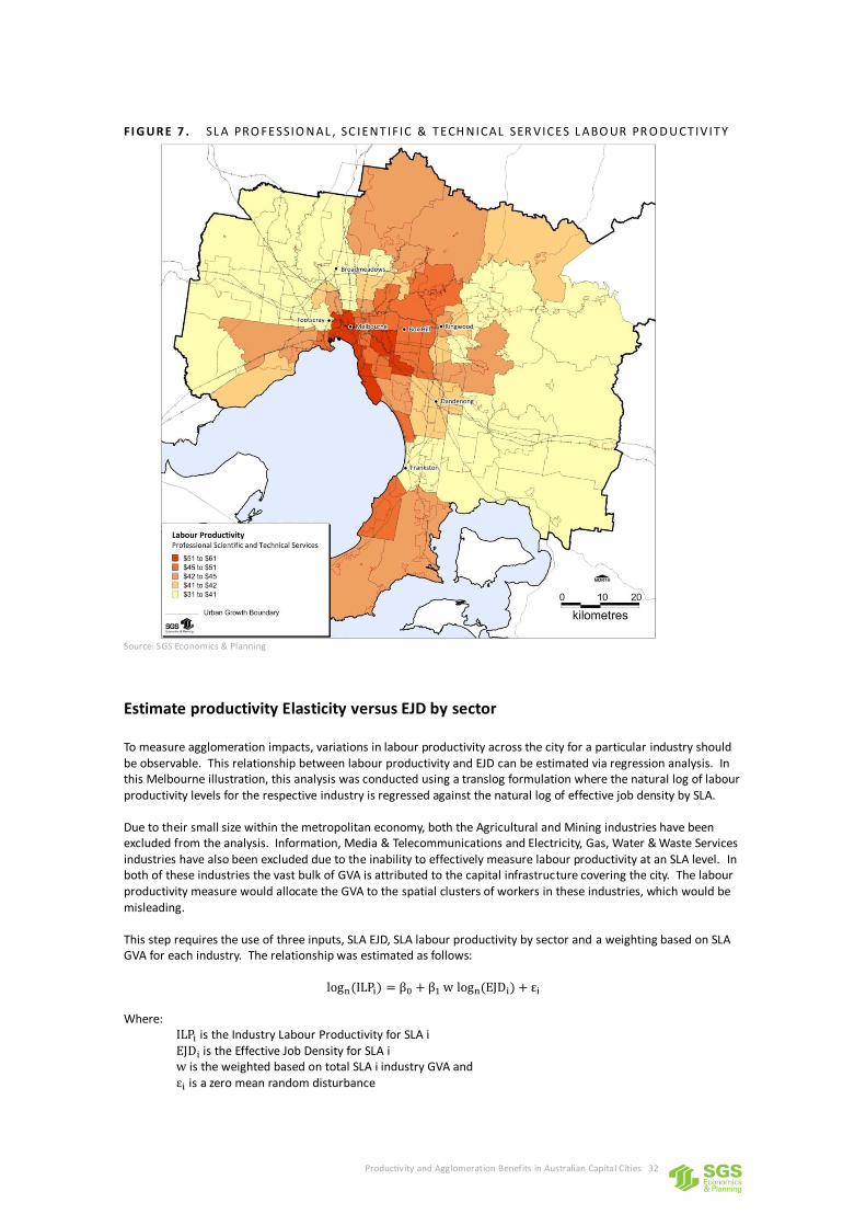
Productivity and Agglomeration Benefits in Australian Capital Cities 32
FI G UR E 7 . SL A PRO FESSIO NAL , SC IENTIFIC & TECH NICAL SER VICES L ABO UR PR O D U CTIV ITY
Source: SGS Economics & Planning
Estimate productivity Elasticity versus EJD by sector
To measure agglomeration impacts, variations in labour productivity across the city for a particular industry should be observable. This relationship between labour productivity and EJD can be estimated via regression analysis. In this Melbourne illustration, this analysis was conducted using a translog formulation where the natural log of labour productivity levels for the respective industry is regressed against the natural log of effective job density by SLA. Due to their small size within the metropolitan economy, both the Agricultural and Mining industries have been excluded from the analysis. Information, Media & Telecommunications and Electricity, Gas, Water & Waste Services industries have also been excluded due to the inability to effectively measure labour productivity at an SLA level. In both of these industries the vast bulk of GVA is attributed to the capital infrastructure covering the city. The labour productivity measure would allocate the GVA to the spatial clusters of workers in these industries, which would be misleading. This step requires the use of three inputs, SLA EJD, SLA labour productivity by sector and a weighting based on SLA GVA for each industry. The relationship was estimated as follows:
Where: is the Industry Labour Productivity for SLA i is the Effective Job Density for SLA i
is the weighted based on total SLA i industry GVA and is a zero mean random disturbance
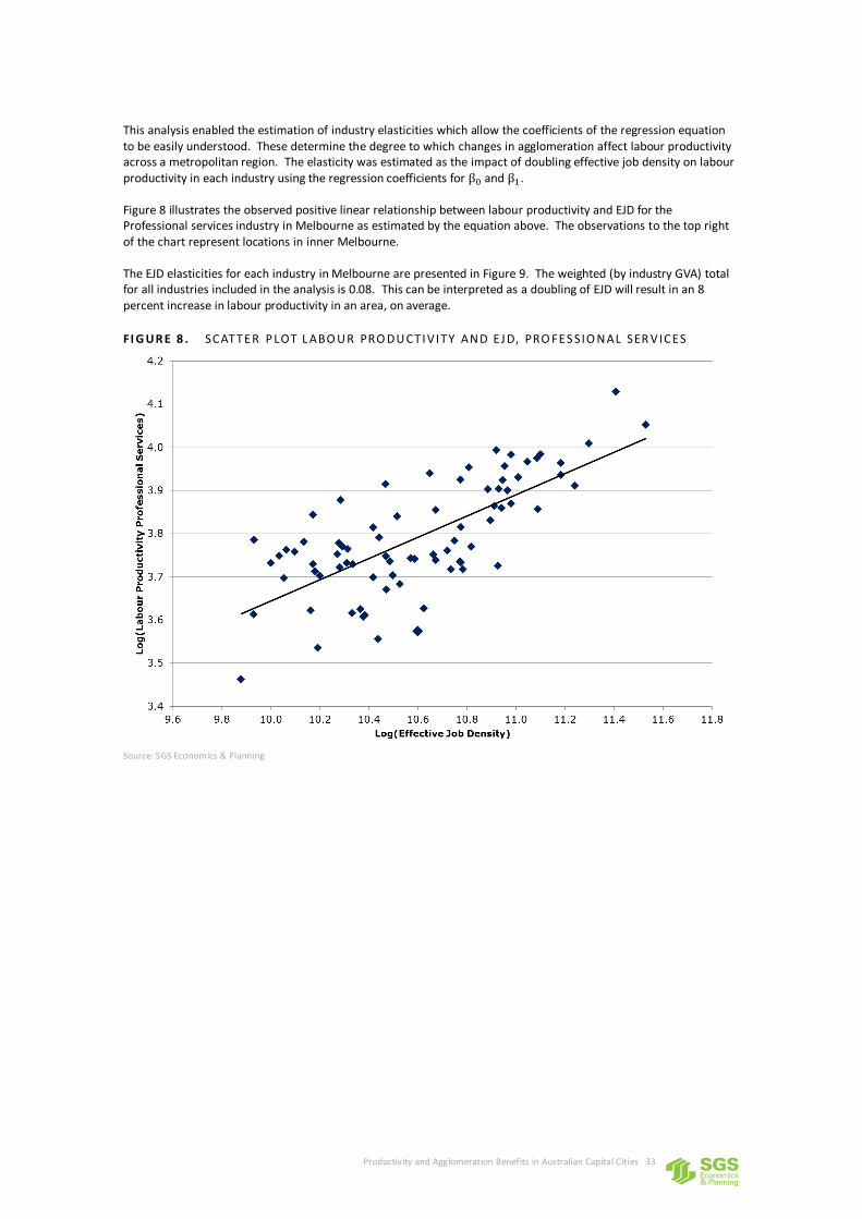
Productivity and Agglomeration Benefits in Australian Capital Cities 33
This analysis enabled the estimation of industry elasticities which allow the coefficients of the regression equation to be easily understood. These determine the degree to which changes in agglomeration affect labour productivity across a metropolitan region. The elasticity was estimated as the impact of doubling effective job density on labour productivity in each industry using the regression coefficients for and . Figure 8 illustrates the observed positive linear relationship between labour productivity and EJD for the Professional services industry in Melbourne as estimated by the equation above. The observations to the top right of the chart represent locations in inner Melbourne. The EJD elasticities for each industry in Melbourne are presented in Figure 9. The weighted (by industry GVA) total for all industries included in the analysis is 0.08. This can be interpreted as a doubling of EJD will result in an 8 percent increase in labour productivity in an area, on average.
FI G UR E 8 . SCATTER P LOT L ABO U R PRO DU CTI V ITY AND EJ D, PRO FES SIO NAL SER VICES
Source: SGS Economics & Planning
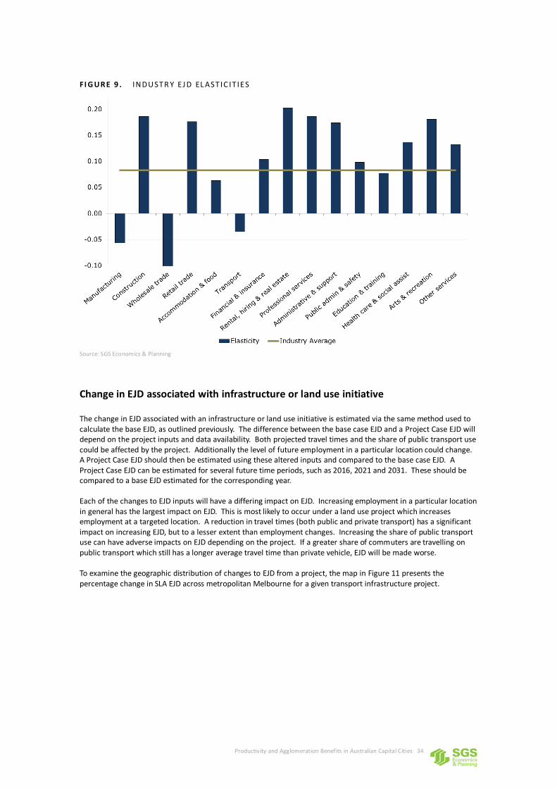
Productivity and Agglomeration Benefits in Australian Capital Cities 34
FI G UR E 9 . INDU STR Y EJ D EL AST IC IT IES
Source: SGS Economics & Planning
Change in EJD associated with infrastructure or land use initiative
The change in EJD associated with an infrastructure or land use initiative is estimated via the same method used to calculate the base EJD, as outlined previously. The difference between the base case EJD and a Project Case EJD will depend on the project inputs and data availability. Both projected travel times and the share of public transport use could be affected by the project. Additionally the level of future employment in a particular location could change. A Project Case EJD should then be estimated using these altered inputs and compared to the base case EJD. A Project Case EJD can be estimated for several future time periods, such as 2016, 2021 and 2031. These should be compared to a base EJD estimated for the corresponding year. Each of the changes to EJD inputs will have a differing impact on EJD. Increasing employment in a particular location in general has the largest impact on EJD. This is most likely to occur under a land use project which increases employment at a targeted location. A reduction in travel times (both public and private transport) has a significant impact on increasing EJD, but to a lesser extent than employment changes. Increasing the share of public transport use can have adverse impacts on EJD depending on the project. If a greater share of commuters are travelling on public transport which still has a longer average travel time than private vehicle, EJD will be made worse. To examine the geographic distribution of changes to EJD from a project, the map in Figure 11 presents the percentage change in SLA EJD across metropolitan Melbourne for a given transport infrastructure project.
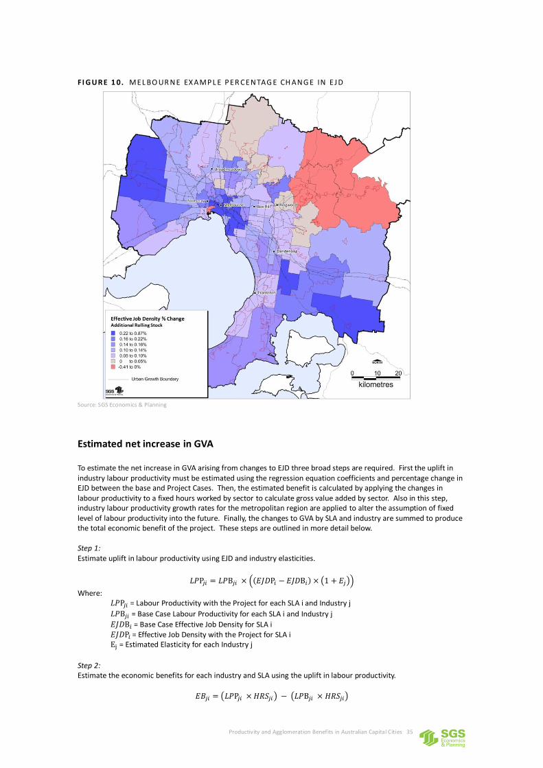
Productivity and Agglomeration Benefits in Australian Capital Cities 35
FI G UR E 1 0. MEL BO UR NE EX AMP L E P ER CENTAG E CH ANG E IN EJ D
Source: SGS Economics & Planning
Estimated net increase in GVA
To estimate the net increase in GVA arising from changes to EJD three broad steps are required. First the uplift in industry labour productivity must be estimated using the regression equation coefficients and percentage change in EJD between the base and Project Cases. Then, the estimated benefit is calculated by applying the changes in labour productivity to a fixed hours worked by sector to calculate gross value added by sector. Also in this step, industry labour productivity growth rates for the metropolitan region are applied to alter the assumption of fixed level of labour productivity into the future. Finally, the changes to GVA by SLA and industry are summed to produce the total economic benefit of the project. These steps are outlined in more detail below. Step 1: Estimate uplift in labour productivity using EJD and industry elasticities.
Where: = Labour Productivity with the Project for each SLA i and Industry j
= Base Case Labour Productivity for each SLA i and Industry j
= Base Case Effective Job Density for SLA i = Effective Job Density with the Project for SLA i = Estimated Elasticity for each Industry j
Step 2: Estimate the economic benefits for each industry and SLA using the uplift in labour productivity.
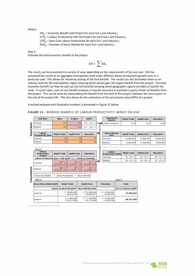
Productivity and Agglomeration Benefits in Australian Capital Cities 36
Where: = Economic Benefit with Project for each SLA i and Industry j
= Labour Productivity with the Project for each SLA i and Industry j
= Base Case Labour Productivity for each SLA i and Industry j
= Number of Hours Worked for each SLA i and Industry j
Step 3: Estimate the total economic benefit of the project
The results can be presented in a variety of ways depending on the requirements of the end user. SGS has presented the results at an aggregate metropolitan level under different labour productivity growth rates in a particular year. This allows for sensitivity testing of the final benefit. The results can also be broken down to an industry level for the metropolitan region showing which sectors gain the largest benefit from the project. The total economic benefit can then be split up into SLA benefits showing which geographic regions are likely to benefit the most. In some cases, such as cost benefit analyses, it may be necessary to estimate a yearly stream of benefits from the project. This can be done by interpolating the benefit from the start of the project, between the future years to the end of the project life. This also allows for the estimation of the net present value (NPV) of a project. A worked example with illustrative numbers is presented in Figure 11 below.
FI G UR E 1 1. WOR K ED EX AMP L E O F L AB OU R PRO DU CTIV ITY IMPACT O N GVA
Source: SGS Economics & Planning
EJD 2031 Base Project Uplift
Geelong 174 175 175 – 174 = 1
Ballarat 110 111 111 – 110 = 1
Labour Productivity: Base
Retail Trade Health Care Education
Geelong 22 32 27
Ballarat 20 30 25
Hours Worked 2031
Retail Trade Health Care Education
Geelong 19,600,000 21,600,000 13,800,000
Ballarat 9,952,000 17,500,000 9,200,000
Regression Results
Retail Trade Health Care Education
Industry Elasticity 0.16 0.13 0.09
Labour Productivity:
ProjectRetail Trade Health Care Education
Labour Productivity Base * EJD Uplift * (1 + Industry Elasticity)
Geelong22 * 1 *
(1+0.16) = 2632 * 1 *
(1+0.13) = 3627 * 1 *
(1+0.09) = 29
Ballarat20 * 1 *
(1+0.16) = 2330 * 1 *
(1+0.13) = 3425 * 1 *
(1+0.09) = 27
Gross Value Added Uplift Retail Trade Health Care Education Total
Labour Productivity Uplift * Hours Worked 2031 Sum of Industry Uplift
Geelong4 * 19,600,000
= 33,413,5934 * 21,600,000
= 34,299,8772 * 13,800,000
= 4,645,89272,359,362
Ballarat3 * 9,952,000= 25,177,898
4 * 17,500,000 = 51,115,648
2 * 9,200,000 = 13,459,238
89,752,784
Labour Productivity: Uplift
Retail Trade Health Care Education
Geelong 26 – 22 = 4 36 – 32 = 4 29 – 27 = 2
Ballarat 23 – 20 = 3 34 – 30 = 4 27 – 25 = 2
Gross Value Added = Labour Productivity * Hours Worked
In
pu
t D
ata
Calc
ula
tion
s
Step 1:
Step 2: Step 3:
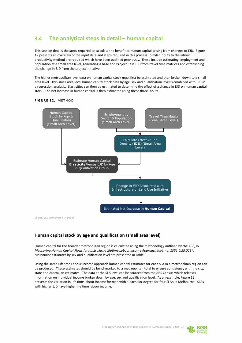
Productivity and Agglomeration Benefits in Australian Capital Cities 37
3.4 The analytical steps in detail – human capital
This section details the steps required to calculate the benefit to human capital arising from changes to EJD. Figure 12 presents an overview of the input data and steps required in this process. Similar inputs to the labour productivity method are required which have been outlined previously. These include estimating employment and population at a small area level, generating a base and Project Case EJD from travel time matrices and establishing the change in EJD from the project initiative. The higher metropolitan level data on human capital stock must first be estimated and then broken down to a small area level. This small area level human capital stock data by age, sex and qualification level is combined with EJD in a regression analysis. Elasticities can then be estimated to determine the effect of a change in EJD on human capital stock. The net increase in human capital is then estimated using these three inputs.
FI G UR E 1 2. METH O D
Source: SGS Economics & Planning
Human capital stock by age and qualification (small area level)
Human capital for the broader metropolitan region is calculated using the methodology outlined by the ABS, in Measuring Human Capital Flows for Australia: A Lifetime Labour Income Approach (cat. no. 1351.0.55.023) . Melbourne estimates by sex and qualification level are presented in Table 9. Using the same Lifetime Labour Income approach human capital estimates for each SLA in a metropolitan region can be produced. These estimates should be benchmarked to a metropolitan total to ensure consistency with the city, state and Australian estimates. The data at the SLA level can be sourced from the ABS Census which releases information on individual income broken down by age, sex and qualification level. As an example, Figure 13 presents the variation in life time labour income for men with a bachelor degree for four SLA’s in Melbourne. SLAs with higher EJD have higher life time labour income.
Employment by Sector & Population (Small Area Level)
Travel Time Matrix(Small Area Level)
Calculate Effective Job Density (EJD) (Small Area
Level)
Human Capital Stock by Age & Qualification
(Small Area Level)
Estimated Net Increase in Human Capital
Estimate Human CapitalElasticity Versus EJD by Age
& Qualification Group
Change in EJD Associated withInfrastructure or Land Use Initiative
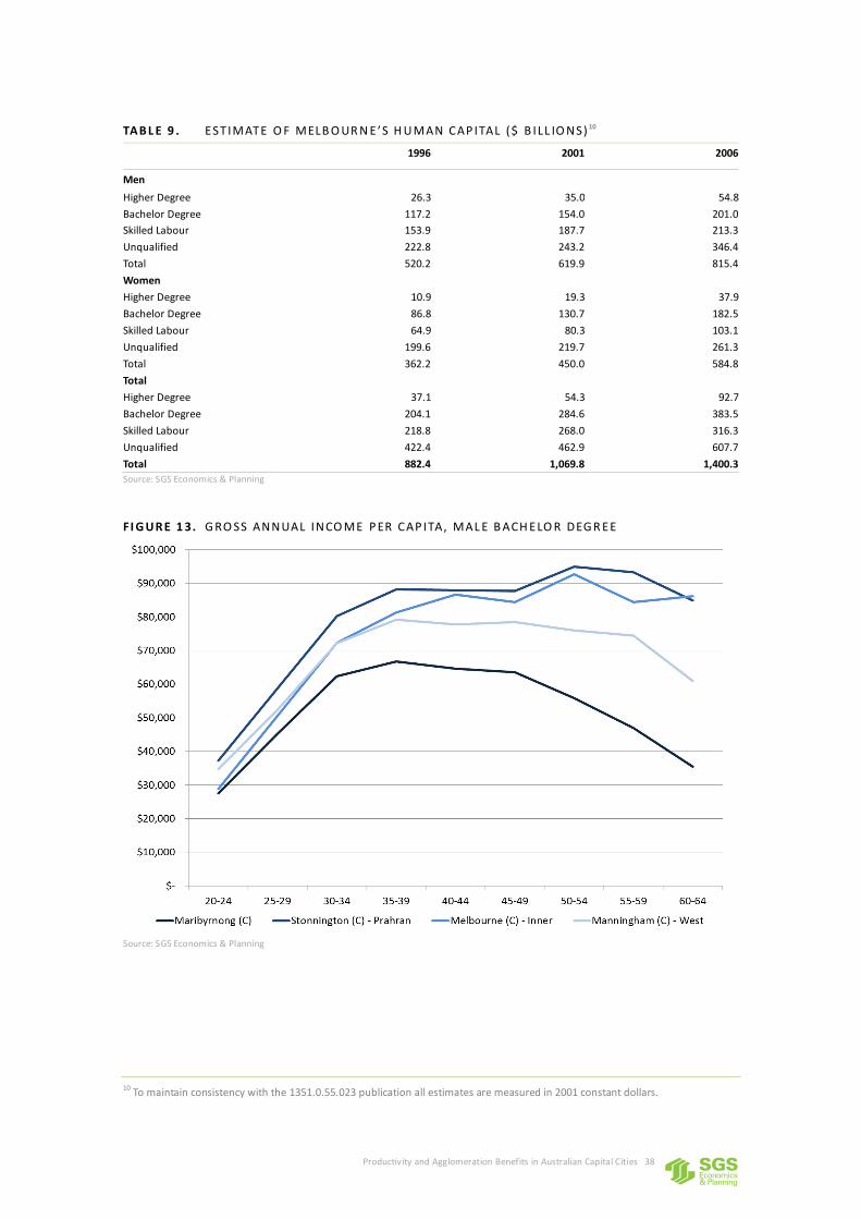
Productivity and Agglomeration Benefits in Australian Capital Cities 38
TAB L E 9 . EST IMATE O F MELB O UR N E ’S H U MAN CAP ITAL ($ B ILL IO NS) 10
1996 2001 2006
Men
Higher Degree 26.3 35.0 54.8
Bachelor Degree 117.2 154.0 201.0
Skilled Labour 153.9 187.7 213.3
Unqualified 222.8 243.2 346.4
Total 520.2 619.9 815.4
Women
Higher Degree 10.9 19.3 37.9
Bachelor Degree 86.8 130.7 182.5
Skilled Labour 64.9 80.3 103.1
Unqualified 199.6 219.7 261.3
Total 362.2 450.0 584.8
Total
Higher Degree 37.1 54.3 92.7
Bachelor Degree 204.1 284.6 383.5
Skilled Labour 218.8 268.0 316.3
Unqualified 422.4 462.9 607.7
Total 882.4 1,069.8 1,400.3
Source: SGS Economics & Planning
FI G UR E 1 3. G RO SS ANNUAL INCO ME P ER CAP ITA, MAL E B ACH ELO R DEG R EE
Source: SGS Economics & Planning
10 To maintain consistency with the 1351.0.55.023 publication all estimates are measured in 2001 constant dollars.
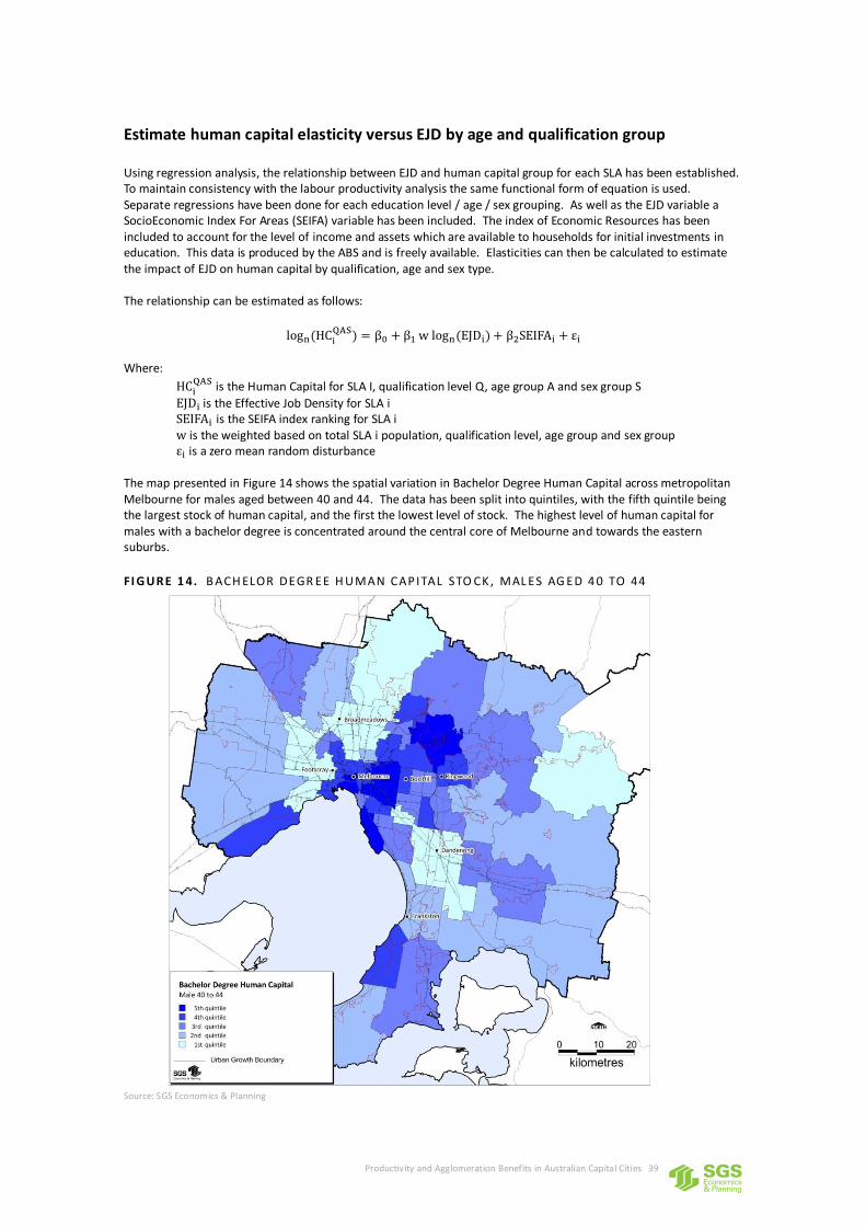
Productivity and Agglomeration Benefits in Australian Capital Cities 39
Estimate human capital elasticity versus EJD by age and qualification group
Using regression analysis, the relationship between EJD and human capital group for each SLA has been established. To maintain consistency with the labour productivity analysis the same functional form of equation is used. Separate regressions have been done for each education level / age / sex grouping. As well as the EJD variable a SocioEconomic Index For Areas (SEIFA) variable has been included. The index of Economic Resources has been included to account for the level of income and assets which are available to households for initial investments in education. This data is produced by the ABS and is freely available. Elasticities can then be calculated to estimate the impact of EJD on human capital by qualification, age and sex type. The relationship can be estimated as follows:
Where:
is the Human Capital for SLA I, qualification level Q, age group A and sex group S
is the Effective Job Density for SLA i is the SEIFA index ranking for SLA i
is the weighted based on total SLA i population, qualification level, age group and sex group is a zero mean random disturbance The map presented in Figure 14 shows the spatial variation in Bachelor Degree Human Capital across metropolitan Melbourne for males aged between 40 and 44. The data has been split into quintiles, with the fifth quintile being the largest stock of human capital, and the first the lowest level of stock. The highest level of human capital for males with a bachelor degree is concentrated around the central core of Melbourne and towards the eastern suburbs.
FI G UR E 1 4. B ACH ELOR DEGR EE H U MAN CAP ITAL STO CK , MAL ES AG ED 4 0 TO 44
Source: SGS Economics & Planning

Productivity and Agglomeration Benefits in Australian Capital Cities 40
Estimated net increase in human capital
To estimate the net increase in GVA from human capital impacts arising from changes to EJD three broad steps are required, similar to the labour productivity method outlined previously. First the uplift in human capital by qualification, age and sex grouping must be estimated using the regression equation coefficients and percentage change in EJD between base and Project Case. Then, the estimated change to human capital is calculated by applying the changes in human capital stock to a fixed population projection by qualification, age and sex grouping. This then allows the calculation of the total human capital uplift across the metropolitan area. Finally, the changes to human capital by SLA and qualification, age and sex grouping are summed. This is then multiplied by a capital services rate which assumes an elasticity between changes to human capital and changes to GVA. These steps are outlined in more detail, below. Step 1: Estimate uplift in human capital using EJD and elasticities.
Where:
= Human Capital with the Project for each SLA i and qualification level Q, age group A and sex group S
= Base Case Human Capital for each SLA i and qualification level Q, age group A and sex group S
= Base Case Effective Job Density for SLA i = Effective Job Density with the Project for SLA i = Estimated Elasticity for each human capital qualification, age and sex grouping
Step 2: Estimate the total human capital benefits for each qualification, age and sex grouping and SLA using the uplift in human capital.
Where:
= Total Human Capital Benefit for each SLA i and qualification level Q, age group A and sex group S
= Human Capital with the Project for each SLA i and qualification level Q, age group A and sex group S
= Base Case Human Capital for each SLA i and qualification level Q, age group A and sex group S
= Population for each SLA i and qualification level Q, age group A and sex group S
Step 3: Estimate the total benefit to GVA of the project
Where: = Economic Benefit to GVA = elasticity of impact of human capital on GVA (9.7%) The results can be presented in a variety of ways. SGS has presented the results at an aggregate metropolitan level under the four main qualification levels (Unqualified, Skilled Labour, Bachelor Degree and Higher Degree). The results can also be broken down to male and female by qualification level. The total economic benefit can then be split up into SLA benefits showing which geographic regions are likely to benefit the most. In some cases, such as cost benefit analyses, it may be necessary to estimate a yearly stream of benefits from the project. This can be done by interpolating the benefit from the start of the project, between the future years to the end of the project life. This also allows for the estimation of the net present value (NPV) of a project. A worked example with illustrative numbers is presented in Figure 15 below.
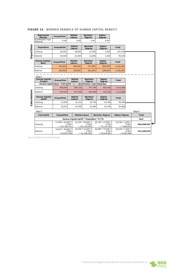
Productivity and Agglomeration Benefits in Australian Capital Cities 41
FI G UR E 1 5. WOR K ED EX AMP L E O F HU MAN CAP ITAL B ENEFI T
Source: SGS Economics & Planning
Human Capital: Base
UnqualifiedSkilled Labour
Bachelor Degree
Higher Degree
Total
Geelong 433,000 538,000 747,000 600,000 2,318,000
Ballarat 192,000 238,000 301,000 298,000 1,029,000
Population UnqualifiedSkilled Labour
Bachelor Degree
Higher Degree
Total
Geelong 60,000 48,000 23,500 3,200 134,700
Ballarat 40,000 22,000 15,000 1,500 78,500
Human Capital:Project
UnqualifiedSkilled Labour
Bachelor Degree
Higher Degree
Total
Human Capital Base * EJD Uplift * (1 + Qualification Type Elasticity)
Geelong 450,830 560,153 777,759 624,706 2,413,448
Ballarat 207,615 257,356 325,480 322,236 1,112,688
Regression Results
UnqualifiedSkilled Labour
Bachelor Degree
Higher Degree
Qualification Type Elasticity
0.09 0.09 0.09 0.09
Total Uplift Unqualified Skilled Labour Bachelor Degree Higher Degree Total
Human Capital Uplift * Population * 9.7% Sum
Geelong17,830 * 60,000 *
0.097= 103,768,721
22,153 * 48,000 * 0.097
= 103,145,629
30,759 * 23,500 * 0.097
= 70,115,782
24,706 * 3,200 * 0.097
= 7,668,820 284,698,951
Ballarat15,615 * 40,000 *
0.097 = 60,587,258
19,356 * 22,000 * 0.097
= 41,306,625
24,480 * 15,000 * 0.097
= 35,618,681
24,236 * 1,500 * 0.097
= 3,526,368141,038,933
In
pu
t D
ata
Calc
ula
tion
s
Step 1:
Step 2: Step 3:
Human Capital:Uplift
UnqualifiedSkilled Labour
Bachelor Degree
Higher Degree
Total
Geelong 17,830 22,153 30,759 24,706 95,448
Ballarat 15,615 19,356 24,480 24,236 83,688
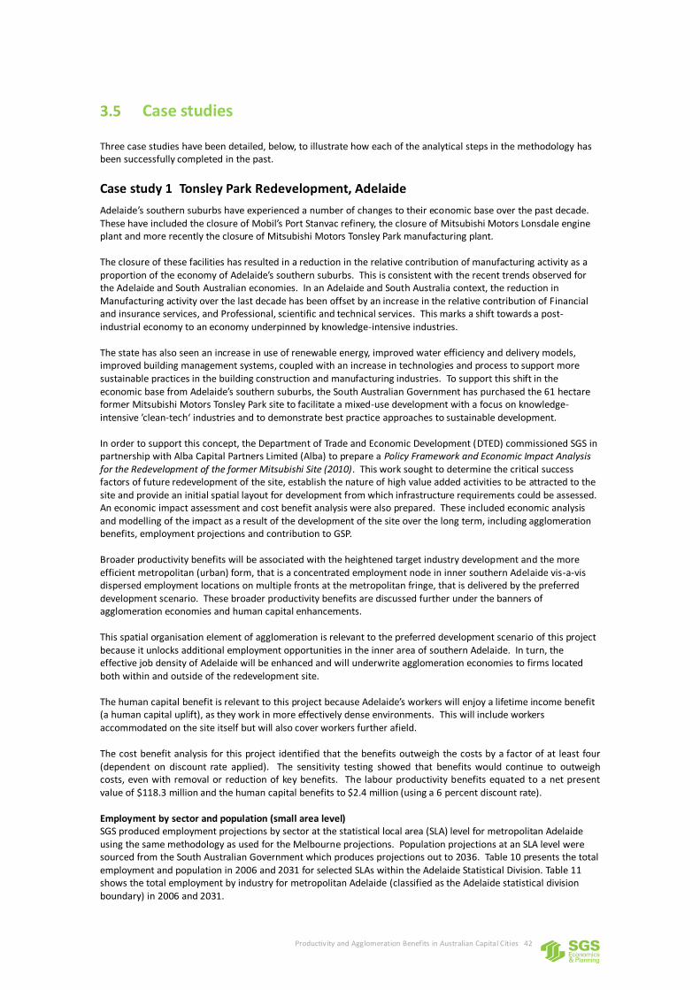
Productivity and Agglomeration Benefits in Australian Capital Cities 42
3.5 Case studies
Three case studies have been detailed, below, to illustrate how each of the analytical steps in the methodology has been successfully completed in the past.
Case study 1 Tonsley Park Redevelopment, Adelaide
Adelaide’s southern suburbs have experienced a number of changes to their economic base over the past decade. These have included the closure of Mobil’s Port Stanvac refinery, the closure of Mitsubishi Motors Lonsdale engine plant and more recently the closure of Mitsubishi Motors Tonsley Park manufacturing plant. The closure of these facilities has resulted in a reduction in the relative contribution of manufacturing activity as a proportion of the economy of Adelaide’s southern suburbs. This is consistent with the recent trends observed for the Adelaide and South Australian economies. In an Adelaide and South Australia context, the reduction in Manufacturing activity over the last decade has been offset by an increase in the relative contribution of Financial and insurance services, and Professional, scientific and technical services. This marks a shift towards a post-industrial economy to an economy underpinned by knowledge-intensive industries. The state has also seen an increase in use of renewable energy, improved water efficiency and delivery models, improved building management systems, coupled with an increase in technologies and process to support more sustainable practices in the building construction and manufacturing industries. To support this shift in the economic base from Adelaide’s southern suburbs, the South Australian Government has purchased the 61 hectare former Mitsubishi Motors Tonsley Park site to facilitate a mixed-use development with a focus on knowledge-intensive ’clean-tech‘ industries and to demonstrate best practice approaches to sustainable development. In order to support this concept, the Department of Trade and Economic Development (DTED) commissioned SGS in partnership with Alba Capital Partners Limited (Alba) to prepare a Policy Framework and Economic Impact Analysis for the Redevelopment of the former Mitsubishi Site (2010). This work sought to determine the critical success factors of future redevelopment of the site, establish the nature of high value added activities to be attracted to the site and provide an initial spatial layout for development from which infrastructure requirements could be assessed. An economic impact assessment and cost benefit analysis were also prepared. These included economic analysis and modelling of the impact as a result of the development of the site over the long term, including agglomeration benefits, employment projections and contribution to GSP. Broader productivity benefits will be associated with the heightened target industry development and the more efficient metropolitan (urban) form, that is a concentrated employment node in inner southern Adelaide vis-a-vis dispersed employment locations on multiple fronts at the metropolitan fringe, that is delivered by the preferred development scenario. These broader productivity benefits are discussed further under the banners of agglomeration economies and human capital enhancements. This spatial organisation element of agglomeration is relevant to the preferred development scenario of this project because it unlocks additional employment opportunities in the inner area of southern Adelaide. In turn, the effective job density of Adelaide will be enhanced and will underwrite agglomeration economies to firms located both within and outside of the redevelopment site. The human capital benefit is relevant to this project because Adelaide’s workers will enjoy a lifetime income benefit (a human capital uplift), as they work in more effectively dense environments. This will include workers accommodated on the site itself but will also cover workers further afield. The cost benefit analysis for this project identified that the benefits outweigh the costs by a factor of at least four (dependent on discount rate applied). The sensitivity testing showed that benefits would continue to outweigh costs, even with removal or reduction of key benefits. The labour productivity benefits equated to a net present value of $118.3 million and the human capital benefits to $2.4 million (using a 6 percent discount rate). Employment by sector and population (small area level) SGS produced employment projections by sector at the statistical local area (SLA) level for metropolitan Adelaide using the same methodology as used for the Melbourne projections. Population projections at an SLA level were sourced from the South Australian Government which produces projections out to 2036. Table 10 presents the total employment and population in 2006 and 2031 for selected SLAs within the Adelaide Statistical Division. Table 11 shows the total employment by industry for metropolitan Adelaide (classified as the Adelaide statistical division boundary) in 2006 and 2031.
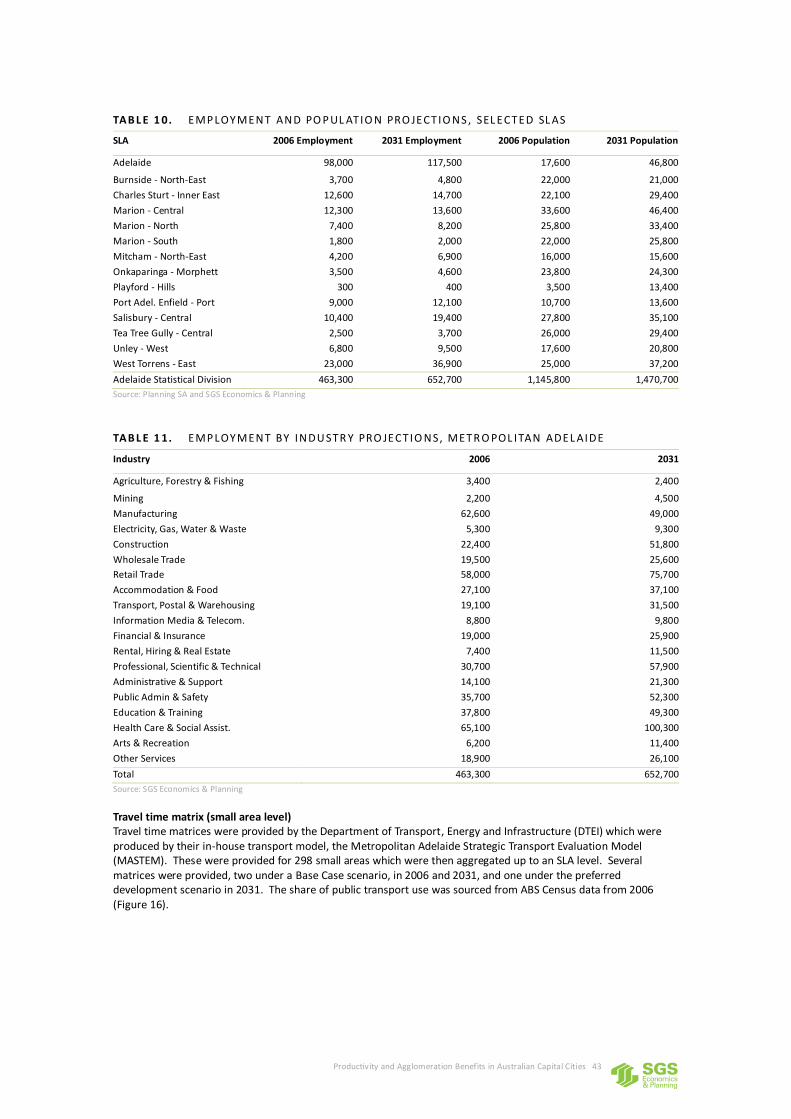
Productivity and Agglomeration Benefits in Australian Capital Cities 43
TAB L E 1 0. EMP LOYMENT AND PO P UL ATIO N PRO JECT IO NS , SEL ECTED SL AS
SLA 2006 Employment 2031 Employment 2006 Population 2031 Population
Adelaide 98,000 117,500 17,600 46,800
Burnside - North-East 3,700 4,800 22,000 21,000
Charles Sturt - Inner East 12,600 14,700 22,100 29,400
Marion - Central 12,300 13,600 33,600 46,400
Marion - North 7,400 8,200 25,800 33,400
Marion - South 1,800 2,000 22,000 25,800
Mitcham - North-East 4,200 6,900 16,000 15,600
Onkaparinga - Morphett 3,500 4,600 23,800 24,300
Playford - Hills 300 400 3,500 13,400
Port Adel. Enfield - Port 9,000 12,100 10,700 13,600
Salisbury - Central 10,400 19,400 27,800 35,100
Tea Tree Gully - Central 2,500 3,700 26,000 29,400
Unley - West 6,800 9,500 17,600 20,800
West Torrens - East 23,000 36,900 25,000 37,200
Adelaide Statistical Division 463,300 652,700 1,145,800 1,470,700
Source: Planning SA and SGS Economics & Planning
TAB L E 1 1. EMP LOYMENT BY INDU STR Y PRO JECT IO NS, METR O POL ITAN ADEL AIDE
Industry 2006 2031
Agriculture, Forestry & Fishing 3,400 2,400
Mining 2,200 4,500
Manufacturing 62,600 49,000
Electricity, Gas, Water & Waste 5,300 9,300
Construction 22,400 51,800
Wholesale Trade 19,500 25,600
Retail Trade 58,000 75,700
Accommodation & Food 27,100 37,100
Transport, Postal & Warehousing 19,100 31,500
Information Media & Telecom. 8,800 9,800
Financial & Insurance 19,000 25,900
Rental, Hiring & Real Estate 7,400 11,500
Professional, Scientific & Technical 30,700 57,900
Administrative & Support 14,100 21,300
Public Admin & Safety 35,700 52,300
Education & Training 37,800 49,300
Health Care & Social Assist. 65,100 100,300
Arts & Recreation 6,200 11,400
Other Services 18,900 26,100
Total 463,300 652,700
Source: SGS Economics & Planning
Travel time matrix (small area level) Travel time matrices were provided by the Department of Transport, Energy and Infrastructure (DTEI) which were produced by their in-house transport model, the Metropolitan Adelaide Strategic Transport Evaluation Model (MASTEM). These were provided for 298 small areas which were then aggregated up to an SLA level. Several matrices were provided, two under a Base Case scenario, in 2006 and 2031, and one under the preferred development scenario in 2031. The share of public transport use was sourced from ABS Census data from 2006 (Figure 16).
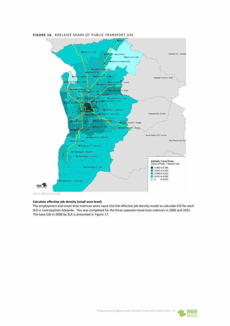
Productivity and Agglomeration Benefits in Australian Capital Cities 44
FI G UR E 1 6. ADEL AIDE SH AR E O F P UBL IC TR ANSP OR T U SE
Source: ABS Census 2006
Calculate effective job density (small area level) The employment and travel time matrices were input into the effective job density model to calculate EJD for each SLA in metropolitan Adelaide. This was completed for the three separate travel time matrices in 2006 and 2031. The base EJD in 2006 by SLA is presented in Figure 17.
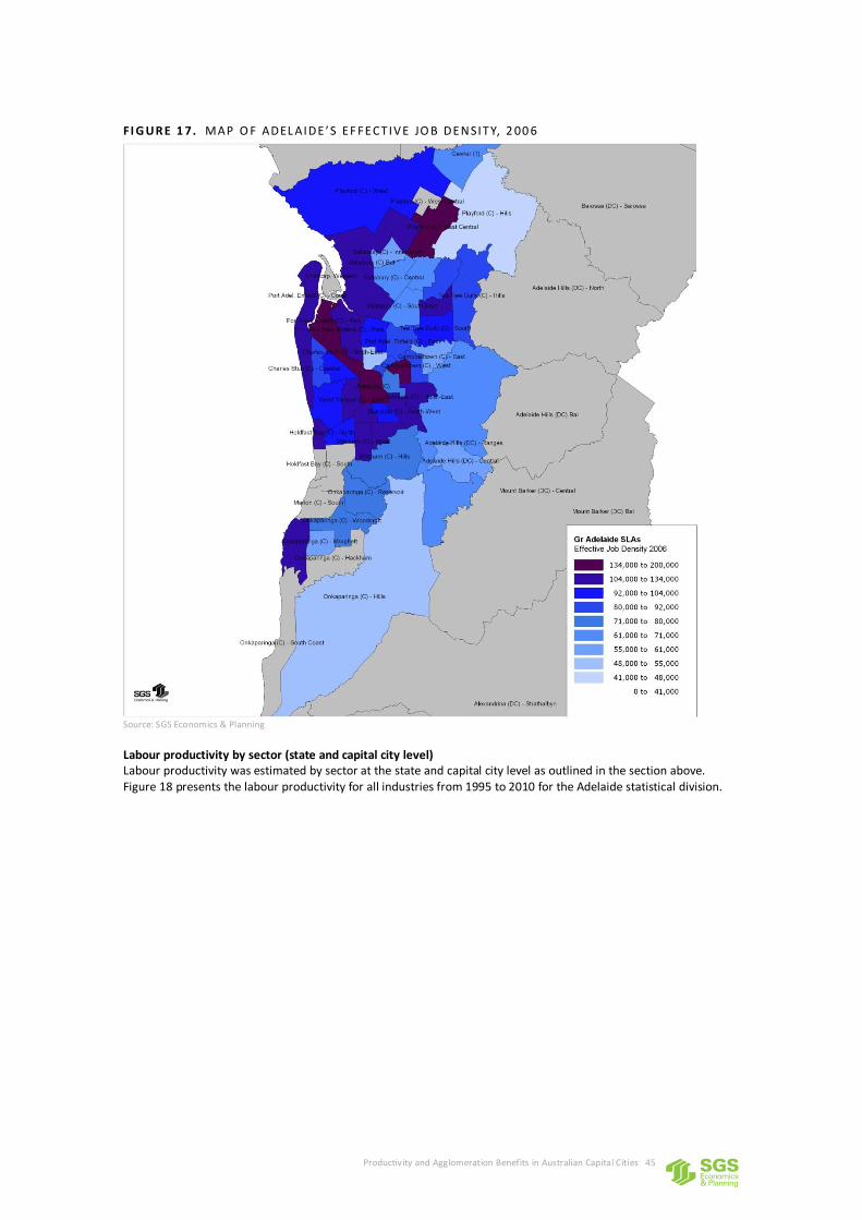
Productivity and Agglomeration Benefits in Australian Capital Cities 45
FI G UR E 1 7. MAP O F ADEL AIDE’S EF FECTIVE JO B DENSITY, 2 00 6
Source: SGS Economics & Planning
Labour productivity by sector (state and capital city level) Labour productivity was estimated by sector at the state and capital city level as outlined in the section above. Figure 18 presents the labour productivity for all industries from 1995 to 2010 for the Adelaide statistical division.
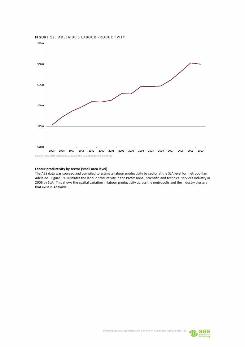
Productivity and Agglomeration Benefits in Australian Capital Cities 46
FI G UR E 1 8. ADEL AIDE’S L ABO UR PR O DU CTIV ITY
Source: ABS State Accounts 5220.0 and SGS Economics & Planning
Labour productivity by sector (small area level) The ABS data was sourced and compiled to estimate labour productivity by sector at the SLA level for metropolitan Adelaide. Figure 19 illustrates the labour productivity in the Professional, scientific and technical services industry in 2006 by SLA. This shows the spatial variation in labour productivity across the metropolis and the industry clusters that exist in Adelaide.
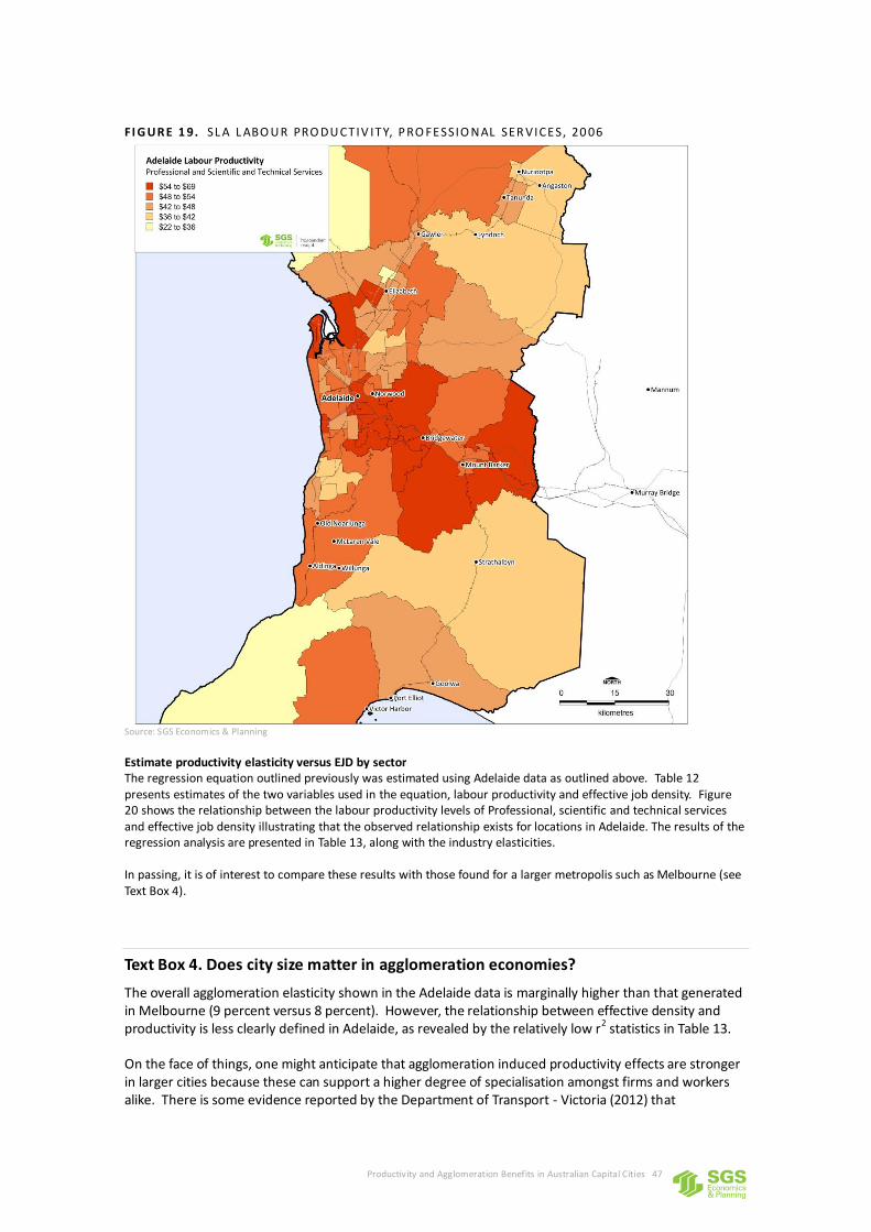
Productivity and Agglomeration Benefits in Australian Capital Cities 47
FI G UR E 1 9. SL A L ABO U R PRO DU CTIV ITY, P RO FESSIO NAL SER VICES, 20 06
Source: SGS Economics & Planning
Estimate productivity elasticity versus EJD by sector The regression equation outlined previously was estimated using Adelaide data as outlined above. Table 12 presents estimates of the two variables used in the equation, labour productivity and effective job density. Figure 20 shows the relationship between the labour productivity levels of Professional, scientific and technical services and effective job density illustrating that the observed relationship exists for locations in Adelaide. The results of the regression analysis are presented in Table 13, along with the industry elasticities. In passing, it is of interest to compare these results with those found for a larger metropolis such as Melbourne (see Text Box 4).
Text Box 4. Does city size matter in agglomeration economies?
The overall agglomeration elasticity shown in the Adelaide data is marginally higher than that generated in Melbourne (9 percent versus 8 percent). However, the relationship between effective density and productivity is less clearly defined in Adelaide, as revealed by the relatively low r2 statistics in Table 13. On the face of things, one might anticipate that agglomeration induced productivity effects are stronger in larger cities because these can support a higher degree of specialisation amongst firms and workers alike. There is some evidence reported by the Department of Transport - Victoria (2012) that
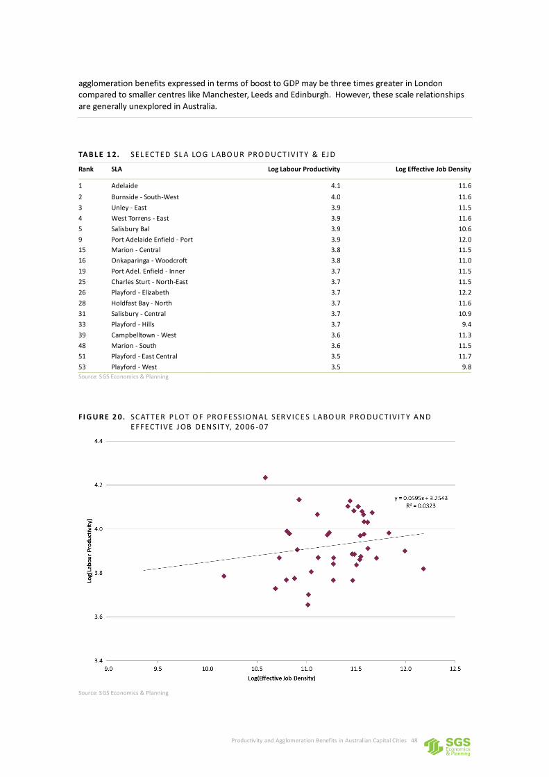
Productivity and Agglomeration Benefits in Australian Capital Cities 48
agglomeration benefits expressed in terms of boost to GDP may be three times greater in London compared to smaller centres like Manchester, Leeds and Edinburgh. However, these scale relationships are generally unexplored in Australia.
TAB L E 1 2. SEL ECTED SL A LO G L ABO U R PRO DU CT IV ITY & EJ D
Rank SLA Log Labour Productivity Log Effective Job Density
1 Adelaide 4.1 11.6
2 Burnside - South-West 4.0 11.6
3 Unley - East 3.9 11.5
4 West Torrens - East 3.9 11.6
5 Salisbury Bal 3.9 10.6
9 Port Adelaide Enfield - Port 3.9 12.0
15 Marion - Central 3.8 11.5
16 Onkaparinga - Woodcroft 3.8 11.0
19 Port Adel. Enfield - Inner 3.7 11.5
25 Charles Sturt - North-East 3.7 11.5
26 Playford - Elizabeth 3.7 12.2
28 Holdfast Bay - North 3.7 11.6
31 Salisbury - Central 3.7 10.9
33 Playford - Hills 3.7 9.4
39 Campbelltown - West 3.6 11.3
48 Marion - South 3.6 11.5
51 Playford - East Central 3.5 11.7
53 Playford - West 3.5 9.8
Source: SGS Economics & Planning
F I G UR E 2 0. SCATTER P LOT O F PRO FESSIO NAL SER VICE S L ABO UR P RO DU CTIV IT Y AND EFFECTIVE J OB DENSIT Y, 20 06 -07
Source: SGS Economics & Planning
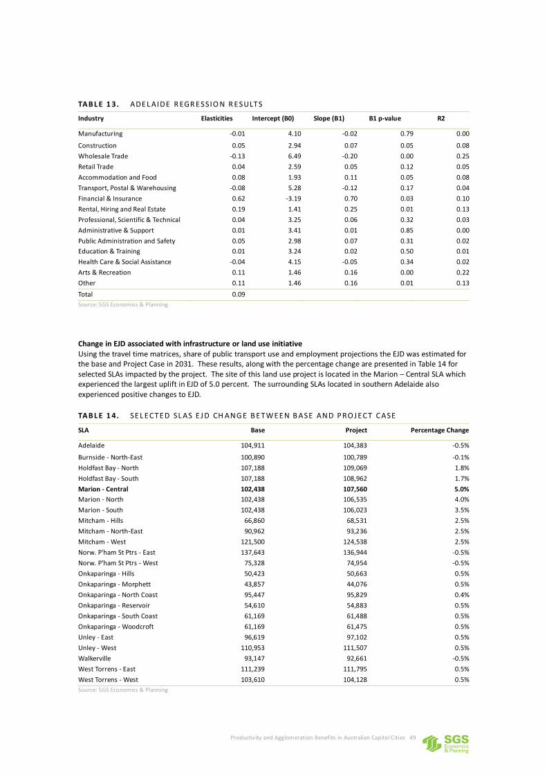
Productivity and Agglomeration Benefits in Australian Capital Cities 49
TAB L E 1 3. ADEL AIDE R EGR ESSIO N R ESULTS
Industry Elasticities Intercept (B0) Slope (B1) B1 p-value R2
Manufacturing -0.01 4.10 -0.02 0.79 0.00
Construction 0.05 2.94 0.07 0.05 0.08
Wholesale Trade -0.13 6.49 -0.20 0.00 0.25
Retail Trade 0.04 2.59 0.05 0.12 0.05
Accommodation and Food 0.08 1.93 0.11 0.05 0.08
Transport, Postal & Warehousing -0.08 5.28 -0.12 0.17 0.04
Financial & Insurance 0.62 -3.19 0.70 0.03 0.10
Rental, Hiring and Real Estate 0.19 1.41 0.25 0.01 0.13
Professional, Scientific & Technical 0.04 3.25 0.06 0.32 0.03
Administrative & Support 0.01 3.41 0.01 0.85 0.00
Public Administration and Safety 0.05 2.98 0.07 0.31 0.02
Education & Training 0.01 3.24 0.02 0.50 0.01
Health Care & Social Assistance -0.04 4.15 -0.05 0.34 0.02
Arts & Recreation 0.11 1.46 0.16 0.00 0.22
Other 0.11 1.46 0.16 0.01 0.13
Total 0.09
Source: SGS Economics & Planning
Change in EJD associated with infrastructure or land use initiative Using the travel time matrices, share of public transport use and employment projections the EJD was estimated for the base and Project Case in 2031. These results, along with the percentage change are presented in Table 14 for selected SLAs impacted by the project. The site of this land use project is located in the Marion – Central SLA which experienced the largest uplift in EJD of 5.0 percent. The surrounding SLAs located in southern Adelaide also experienced positive changes to EJD.
TAB L E 1 4. SEL ECTED SL AS E J D CH ANG E B ETWEEN B ASE AND P RO J ECT CASE
SLA Base Project Percentage Change
Adelaide 104,911 104,383 -0.5%
Burnside - North-East 100,890 100,789 -0.1%
Holdfast Bay - North 107,188 109,069 1.8%
Holdfast Bay - South 107,188 108,962 1.7%
Marion - Central 102,438 107,560 5.0%
Marion - North 102,438 106,535 4.0%
Marion - South 102,438 106,023 3.5%
Mitcham - Hills 66,860 68,531 2.5%
Mitcham - North-East 90,962 93,236 2.5%
Mitcham - West 121,500 124,538 2.5%
Norw. P'ham St Ptrs - East 137,643 136,944 -0.5%
Norw. P'ham St Ptrs - West 75,328 74,954 -0.5%
Onkaparinga - Hills 50,423 50,663 0.5%
Onkaparinga - Morphett 43,857 44,076 0.5%
Onkaparinga - North Coast 95,447 95,829 0.4%
Onkaparinga - Reservoir 54,610 54,883 0.5%
Onkaparinga - South Coast 61,169 61,488 0.5%
Onkaparinga - Woodcroft 61,169 61,475 0.5%
Unley - East 96,619 97,102 0.5%
Unley - West 110,953 111,507 0.5%
Walkerville 93,147 92,661 -0.5%
West Torrens - East 111,239 111,795 0.5%
West Torrens - West 103,610 104,128 0.5%
Source: SGS Economics & Planning
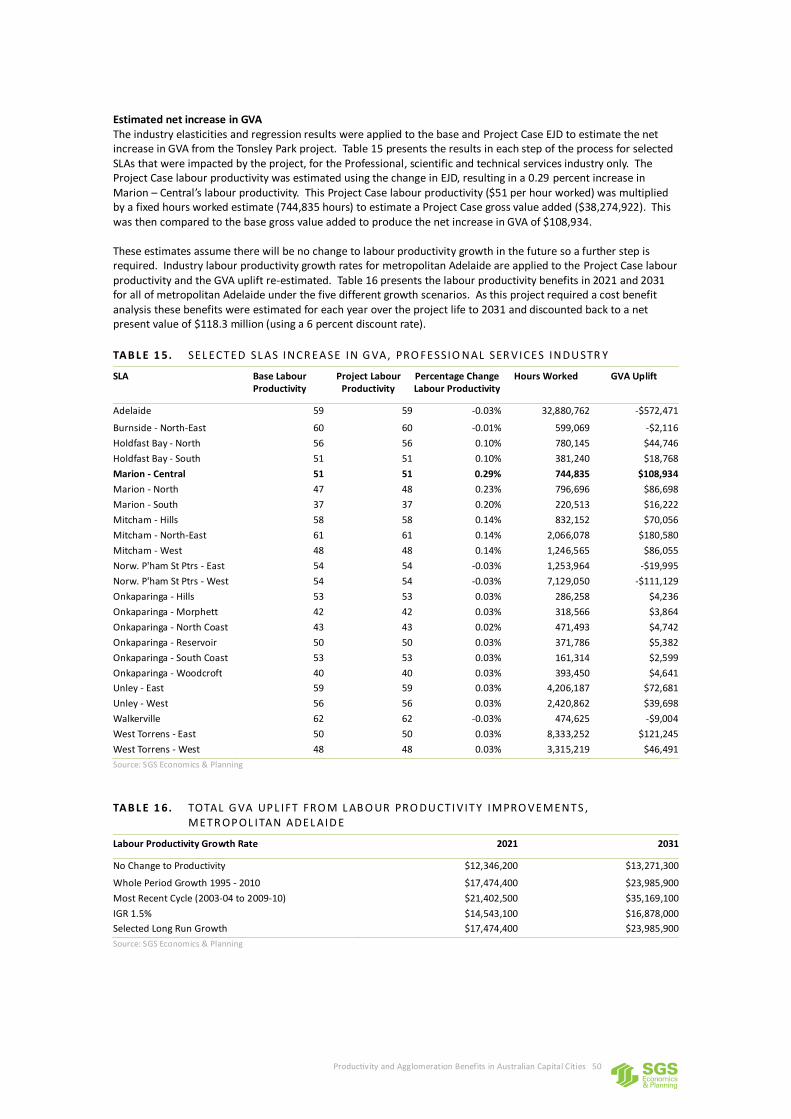
Productivity and Agglomeration Benefits in Australian Capital Cities 50
Estimated net increase in GVA The industry elasticities and regression results were applied to the base and Project Case EJD to estimate the net increase in GVA from the Tonsley Park project. Table 15 presents the results in each step of the process for selected SLAs that were impacted by the project, for the Professional, scientific and technical services industry only. The Project Case labour productivity was estimated using the change in EJD, resulting in a 0.29 percent increase in Marion – Central’s labour productivity. This Project Case labour productivity ($51 per hour worked) was multiplied by a fixed hours worked estimate (744,835 hours) to estimate a Project Case gross value added ($38,274,922). This was then compared to the base gross value added to produce the net increase in GVA of $108,934. These estimates assume there will be no change to labour productivity growth in the future so a further step is required. Industry labour productivity growth rates for metropolitan Adelaide are applied to the Project Case labour productivity and the GVA uplift re-estimated. Table 16 presents the labour productivity benefits in 2021 and 2031 for all of metropolitan Adelaide under the five different growth scenarios. As this project required a cost benefit analysis these benefits were estimated for each year over the project life to 2031 and discounted back to a net present value of $118.3 million (using a 6 percent discount rate).
TAB L E 1 5. SEL ECTED SL AS INCR EA SE IN G VA, PRO FESSIO NAL SER VICES INDU STR Y
SLA Base Labour Productivity
Project Labour Productivity
Percentage Change Labour Productivity
Hours Worked GVA Uplift
Adelaide 59 59 -0.03% 32,880,762 -$572,471
Burnside - North-East 60 60 -0.01% 599,069 -$2,116
Holdfast Bay - North 56 56 0.10% 780,145 $44,746
Holdfast Bay - South 51 51 0.10% 381,240 $18,768
Marion - Central 51 51 0.29% 744,835 $108,934
Marion - North 47 48 0.23% 796,696 $86,698
Marion - South 37 37 0.20% 220,513 $16,222
Mitcham - Hills 58 58 0.14% 832,152 $70,056
Mitcham - North-East 61 61 0.14% 2,066,078 $180,580
Mitcham - West 48 48 0.14% 1,246,565 $86,055
Norw. P'ham St Ptrs - East 54 54 -0.03% 1,253,964 -$19,995
Norw. P'ham St Ptrs - West 54 54 -0.03% 7,129,050 -$111,129
Onkaparinga - Hills 53 53 0.03% 286,258 $4,236
Onkaparinga - Morphett 42 42 0.03% 318,566 $3,864
Onkaparinga - North Coast 43 43 0.02% 471,493 $4,742
Onkaparinga - Reservoir 50 50 0.03% 371,786 $5,382
Onkaparinga - South Coast 53 53 0.03% 161,314 $2,599
Onkaparinga - Woodcroft 40 40 0.03% 393,450 $4,641
Unley - East 59 59 0.03% 4,206,187 $72,681
Unley - West 56 56 0.03% 2,420,862 $39,698
Walkerville 62 62 -0.03% 474,625 -$9,004
West Torrens - East 50 50 0.03% 8,333,252 $121,245
West Torrens - West 48 48 0.03% 3,315,219 $46,491
Source: SGS Economics & Planning
TAB L E 1 6. TOTAL G VA UP L IFT FRO M L AB O UR PRO DU CTI V ITY IMPRO VEMENTS , METR OP OL ITAN ADEL AID E
Labour Productivity Growth Rate 2021 2031
No Change to Productivity $12,346,200 $13,271,300
Whole Period Growth 1995 - 2010 $17,474,400 $23,985,900
Most Recent Cycle (2003-04 to 2009-10) $21,402,500 $35,169,100
IGR 1.5% $14,543,100 $16,878,000
Selected Long Run Growth $17,474,400 $23,985,900
Source: SGS Economics & Planning
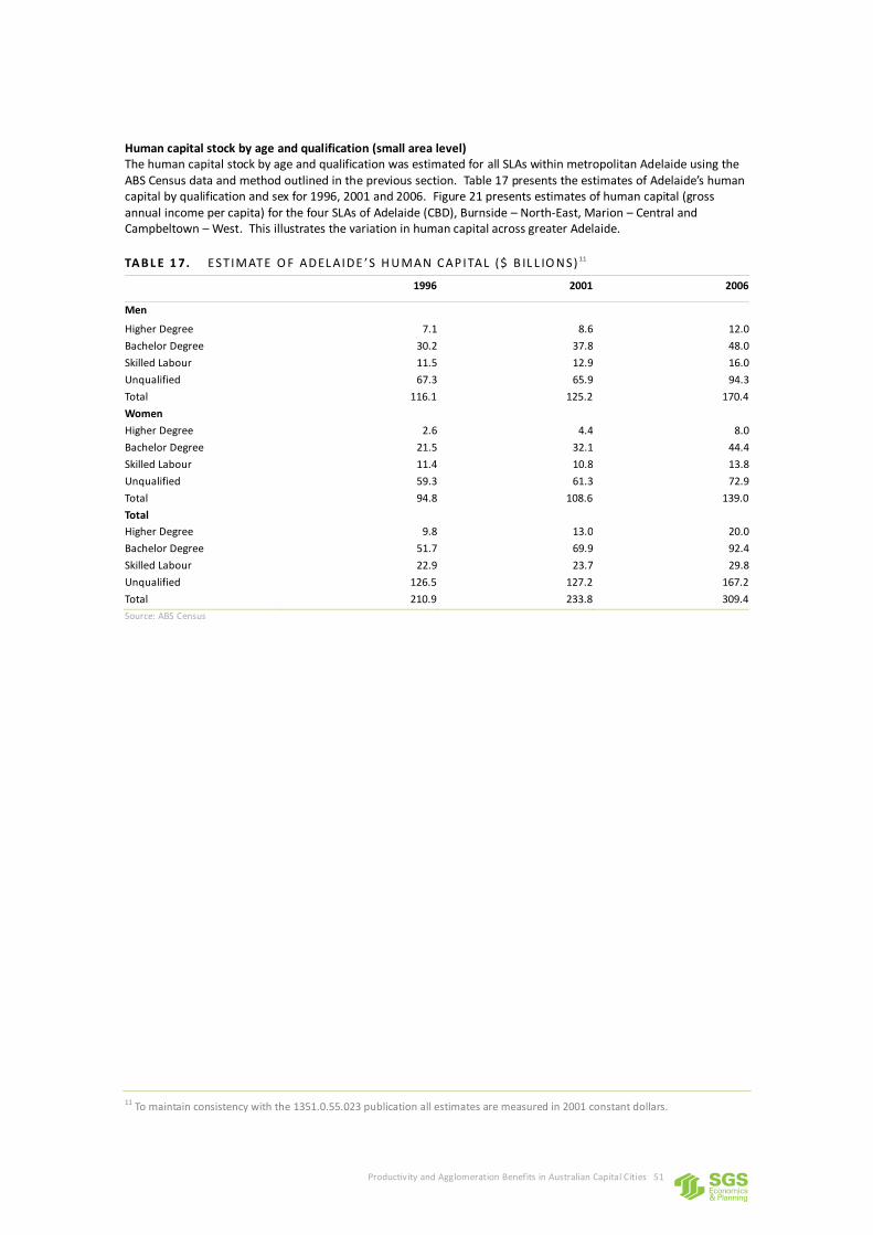
Productivity and Agglomeration Benefits in Australian Capital Cities 51
Human capital stock by age and qualification (small area level) The human capital stock by age and qualification was estimated for all SLAs within metropolitan Adelaide using the ABS Census data and method outlined in the previous section. Table 17 presents the estimates of Adelaide’s human capital by qualification and sex for 1996, 2001 and 2006. Figure 21 presents estimates of human capital (gross annual income per capita) for the four SLAs of Adelaide (CBD), Burnside – North-East, Marion – Central and Campbeltown – West. This illustrates the variation in human capital across greater Adelaide.
TAB L E 1 7. EST IMATE O F ADEL AIDE ’ S H U MAN CAP ITAL ($ B IL L IO NS) 11
1996 2001 2006
Men
Higher Degree 7.1 8.6 12.0
Bachelor Degree 30.2 37.8 48.0
Skilled Labour 11.5 12.9 16.0
Unqualified 67.3 65.9 94.3
Total 116.1 125.2 170.4
Women
Higher Degree 2.6 4.4 8.0
Bachelor Degree 21.5 32.1 44.4
Skilled Labour 11.4 10.8 13.8
Unqualified 59.3 61.3 72.9
Total 94.8 108.6 139.0
Total
Higher Degree 9.8 13.0 20.0
Bachelor Degree 51.7 69.9 92.4
Skilled Labour 22.9 23.7 29.8
Unqualified 126.5 127.2 167.2
Total 210.9 233.8 309.4
Source: ABS Census
11 To maintain consistency with the 1351.0.55.023 publication all estimates are measured in 2001 constant dollars.
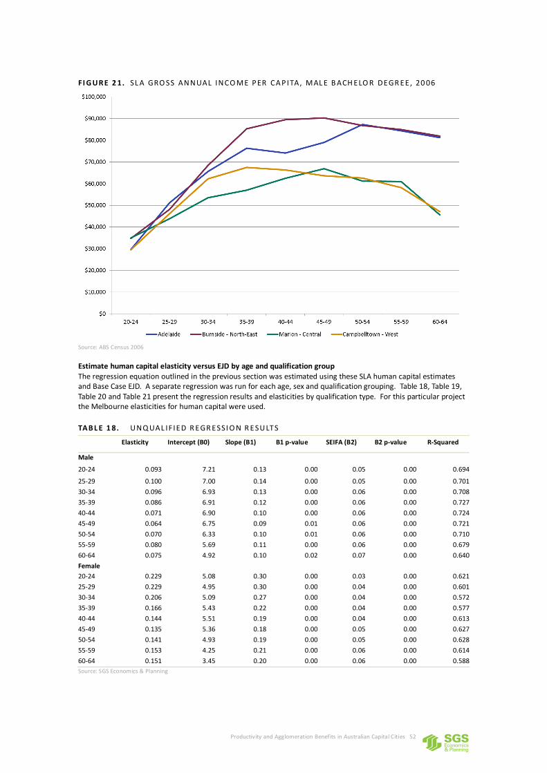
Productivity and Agglomeration Benefits in Australian Capital Cities 52
FI G UR E 2 1. SL A GRO SS ANNUAL INCO ME P ER CA P ITA, MAL E B ACH ELO R DEGR EE, 20 06
Source: ABS Census 2006
Estimate human capital elasticity versus EJD by age and qualification group The regression equation outlined in the previous section was estimated using these SLA human capital estimates and Base Case EJD. A separate regression was run for each age, sex and qualification grouping. Table 18, Table 19, Table 20 and Table 21 present the regression results and elasticities by qualification type. For this particular project the Melbourne elasticities for human capital were used.
TAB L E 1 8. U NQ UAL IFIED R EGR ESSI O N R ESU LTS
Elasticity Intercept (B0) Slope (B1) B1 p-value SEIFA (B2) B2 p-value R-Squared
Male
20-24 0.093 7.21 0.13 0.00 0.05 0.00 0.694
25-29 0.100 7.00 0.14 0.00 0.05 0.00 0.701
30-34 0.096 6.93 0.13 0.00 0.06 0.00 0.708
35-39 0.086 6.91 0.12 0.00 0.06 0.00 0.727
40-44 0.071 6.90 0.10 0.00 0.06 0.00 0.724
45-49 0.064 6.75 0.09 0.01 0.06 0.00 0.721
50-54 0.070 6.33 0.10 0.01 0.06 0.00 0.710
55-59 0.080 5.69 0.11 0.00 0.06 0.00 0.679
60-64 0.075 4.92 0.10 0.02 0.07 0.00 0.640
Female
20-24 0.229 5.08 0.30 0.00 0.03 0.00 0.621
25-29 0.229 4.95 0.30 0.00 0.04 0.00 0.601
30-34 0.206 5.09 0.27 0.00 0.04 0.00 0.572
35-39 0.166 5.43 0.22 0.00 0.04 0.00 0.577
40-44 0.144 5.51 0.19 0.00 0.04 0.00 0.613
45-49 0.135 5.36 0.18 0.00 0.05 0.00 0.627
50-54 0.141 4.93 0.19 0.00 0.05 0.00 0.628
55-59 0.153 4.25 0.21 0.00 0.06 0.00 0.614
60-64 0.151 3.45 0.20 0.00 0.06 0.00 0.588
Source: SGS Economics & Planning
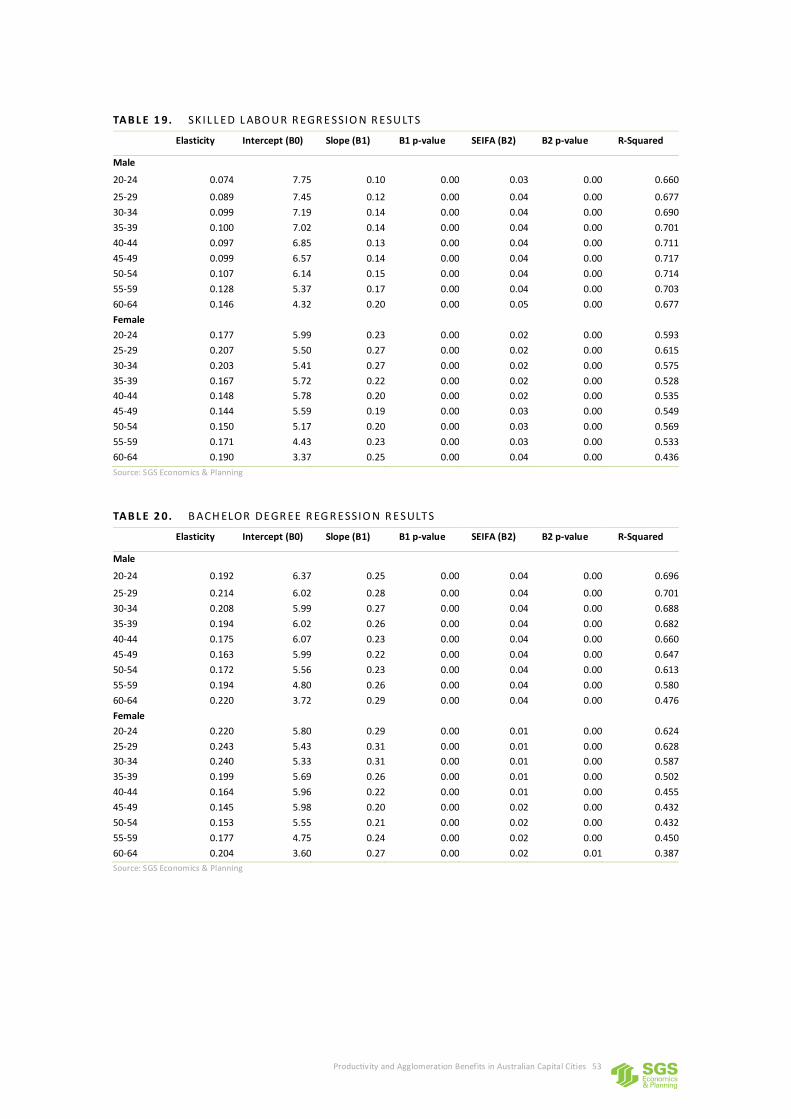
Productivity and Agglomeration Benefits in Australian Capital Cities 53
TAB L E 1 9. SK IL L ED L ABO U R R EGR E SSIO N R ESU LTS
Elasticity Intercept (B0) Slope (B1) B1 p-value SEIFA (B2) B2 p-value R-Squared
Male
20-24 0.074 7.75 0.10 0.00 0.03 0.00 0.660
25-29 0.089 7.45 0.12 0.00 0.04 0.00 0.677
30-34 0.099 7.19 0.14 0.00 0.04 0.00 0.690
35-39 0.100 7.02 0.14 0.00 0.04 0.00 0.701
40-44 0.097 6.85 0.13 0.00 0.04 0.00 0.711
45-49 0.099 6.57 0.14 0.00 0.04 0.00 0.717
50-54 0.107 6.14 0.15 0.00 0.04 0.00 0.714
55-59 0.128 5.37 0.17 0.00 0.04 0.00 0.703
60-64 0.146 4.32 0.20 0.00 0.05 0.00 0.677
Female
20-24 0.177 5.99 0.23 0.00 0.02 0.00 0.593
25-29 0.207 5.50 0.27 0.00 0.02 0.00 0.615
30-34 0.203 5.41 0.27 0.00 0.02 0.00 0.575
35-39 0.167 5.72 0.22 0.00 0.02 0.00 0.528
40-44 0.148 5.78 0.20 0.00 0.02 0.00 0.535
45-49 0.144 5.59 0.19 0.00 0.03 0.00 0.549
50-54 0.150 5.17 0.20 0.00 0.03 0.00 0.569
55-59 0.171 4.43 0.23 0.00 0.03 0.00 0.533
60-64 0.190 3.37 0.25 0.00 0.04 0.00 0.436
Source: SGS Economics & Planning
TAB L E 2 0. B ACH ELOR DEGR EE R EG R ESSIO N R ESULTS
Elasticity Intercept (B0) Slope (B1) B1 p-value SEIFA (B2) B2 p-value R-Squared
Male
20-24 0.192 6.37 0.25 0.00 0.04 0.00 0.696
25-29 0.214 6.02 0.28 0.00 0.04 0.00 0.701
30-34 0.208 5.99 0.27 0.00 0.04 0.00 0.688
35-39 0.194 6.02 0.26 0.00 0.04 0.00 0.682
40-44 0.175 6.07 0.23 0.00 0.04 0.00 0.660
45-49 0.163 5.99 0.22 0.00 0.04 0.00 0.647
50-54 0.172 5.56 0.23 0.00 0.04 0.00 0.613
55-59 0.194 4.80 0.26 0.00 0.04 0.00 0.580
60-64 0.220 3.72 0.29 0.00 0.04 0.00 0.476
Female
20-24 0.220 5.80 0.29 0.00 0.01 0.00 0.624
25-29 0.243 5.43 0.31 0.00 0.01 0.00 0.628
30-34 0.240 5.33 0.31 0.00 0.01 0.00 0.587
35-39 0.199 5.69 0.26 0.00 0.01 0.00 0.502
40-44 0.164 5.96 0.22 0.00 0.01 0.00 0.455
45-49 0.145 5.98 0.20 0.00 0.02 0.00 0.432
50-54 0.153 5.55 0.21 0.00 0.02 0.00 0.432
55-59 0.177 4.75 0.24 0.00 0.02 0.00 0.450
60-64 0.204 3.60 0.27 0.00 0.02 0.01 0.387
Source: SGS Economics & Planning
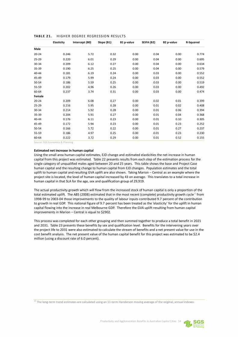
Productivity and Agglomeration Benefits in Australian Capital Cities 54
TAB L E 2 1. H IGH ER DEG R EE REGR ESSIO N RESU LTS
Elasticity Intercept (B0) Slope (B1) B1 p-value SEIFA (B2) B2 p-value R-Squared
Male
20-24 0.246 5.72 0.32 0.00 0.04 0.00 0.774
25-29 0.220 6.01 0.29 0.00 0.04 0.00 0.695
30-34 0.209 6.12 0.27 0.00 0.04 0.00 0.634
35-39 0.190 6.25 0.25 0.00 0.04 0.00 0.579
40-44 0.181 6.19 0.24 0.00 0.03 0.00 0.552
45-49 0.179 5.99 0.24 0.00 0.03 0.00 0.552
50-54 0.186 5.59 0.25 0.00 0.03 0.00 0.519
55-59 0.202 4.96 0.26 0.00 0.03 0.00 0.492
60-64 0.237 3.74 0.31 0.00 0.03 0.00 0.474
Female
20-24 0.209 6.08 0.27 0.00 0.02 0.01 0.399
25-29 0.216 5.95 0.28 0.00 0.01 0.02 0.408
30-34 0.214 5.92 0.28 0.00 0.01 0.06 0.394
35-39 0.204 5.91 0.27 0.00 0.01 0.04 0.368
40-44 0.176 6.11 0.23 0.00 0.01 0.10 0.305
45-49 0.172 5.94 0.23 0.00 0.01 0.23 0.252
50-54 0.166 5.72 0.22 0.00 0.01 0.27 0.237
55-59 0.186 4.97 0.25 0.00 0.01 0.23 0.230
60-64 0.222 3.72 0.29 0.00 0.01 0.52 0.155
Source: SGS Economics & Planning
Estimated net increase in human capital Using the small area human capital estimates, EJD change and estimated elasticities the net increase in human capital from this project was estimated. Table 22 presents results from each step of the estimation process for the single category of unqualified males aged between 20 and 25 years. This table shows the base and Project Case human capital and the resulting change to human capital from EJD changes. Population estimates and the total uplift to human capital and resulting GVA uplift are also shown. Taking Marion – Central as an example where the project site is located, the level of human capital increased by 43 on average. This translates to a total increase in human capital in that SLA for the age, sex and qualification group of 29,919. The actual productivity growth which will flow from the increased stock of human capital is only a proportion of the total estimated uplift. The ABS (2008) estimated that in the most recent (complete) productivity growth cycle12 from 1998-99 to 2003-04 those improvements to the quality of labour inputs contributed 9.7 percent of the contribution to growth in real GDP. This national figure of 9.7 percent has been treated as the ‘elasticity’ for the uplift in human capital flowing into the increase in real Melbourne GDP. Therefore the GVA uplift resulting from human capital improvements in Marion – Central is equal to $2902. This process was completed for each other grouping and then summed together to produce a total benefit in 2021 and 2031. Table 23 presents these benefits by sex and qualification level. Benefits for the intervening years over the project life to 2031 were also estimated to calculate the stream of benefits and a net present value for use in the cost benefit analysis. The net present value of the human capital benefit for this project was estimated to be $2.4 million (using a discount rate of 6.0 percent).
12 The long-term trend estimates are calculated using an 11-term Henderson moving average of the original, annual indexes
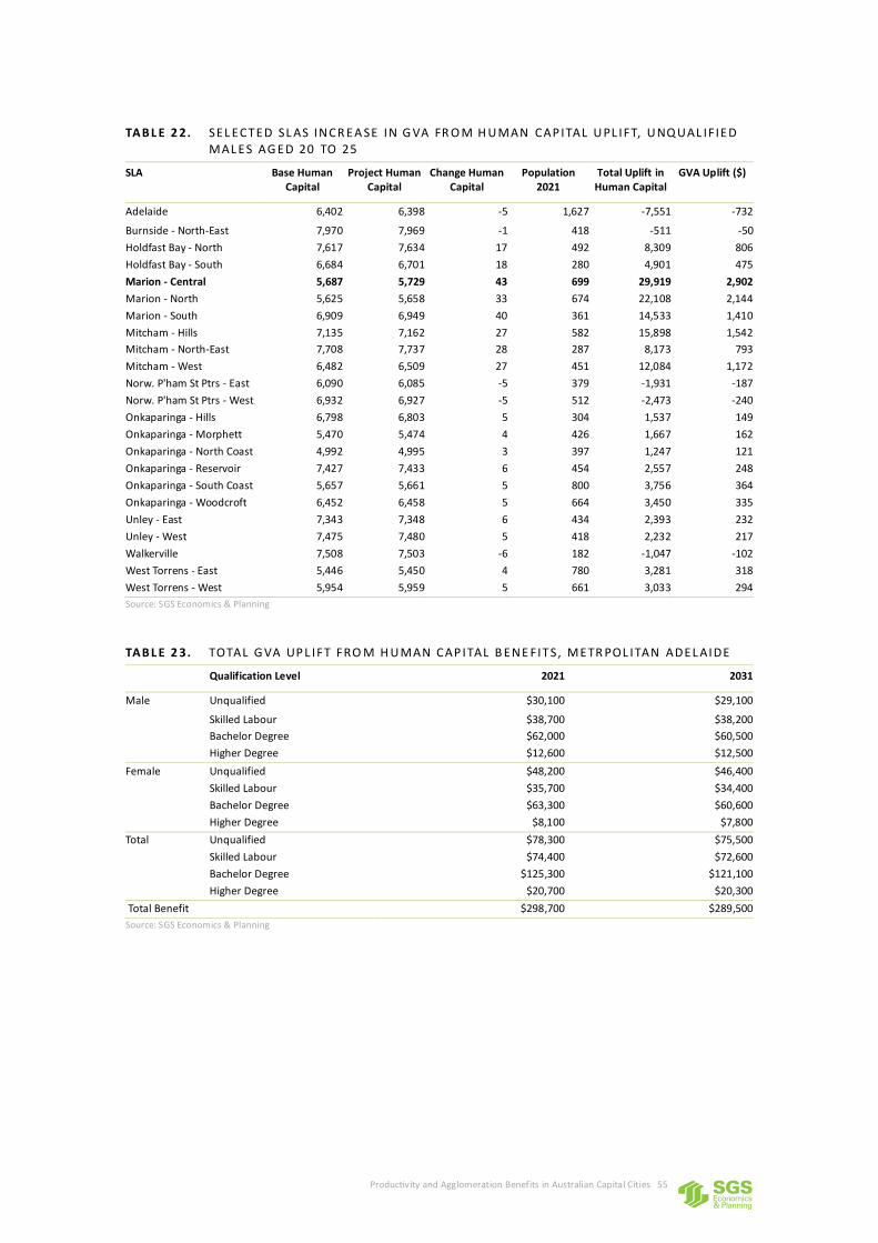
Productivity and Agglomeration Benefits in Australian Capital Cities 55
TAB L E 2 2. SEL ECTED SL AS INCR EA SE IN G VA FR O M H U MAN CAP ITAL U PL IFT, U NQ UAL IFIED MAL ES AG ED 20 TO 25
SLA Base Human Capital
Project Human Capital
Change Human Capital
Population 2021
Total Uplift in Human Capital
GVA Uplift ($)
Adelaide 6,402 6,398 -5 1,627 -7,551 -732
Burnside - North-East 7,970 7,969 -1 418 -511 -50
Holdfast Bay - North 7,617 7,634 17 492 8,309 806
Holdfast Bay - South 6,684 6,701 18 280 4,901 475
Marion - Central 5,687 5,729 43 699 29,919 2,902
Marion - North 5,625 5,658 33 674 22,108 2,144
Marion - South 6,909 6,949 40 361 14,533 1,410
Mitcham - Hills 7,135 7,162 27 582 15,898 1,542
Mitcham - North-East 7,708 7,737 28 287 8,173 793
Mitcham - West 6,482 6,509 27 451 12,084 1,172
Norw. P'ham St Ptrs - East 6,090 6,085 -5 379 -1,931 -187
Norw. P'ham St Ptrs - West 6,932 6,927 -5 512 -2,473 -240
Onkaparinga - Hills 6,798 6,803 5 304 1,537 149
Onkaparinga - Morphett 5,470 5,474 4 426 1,667 162
Onkaparinga - North Coast 4,992 4,995 3 397 1,247 121
Onkaparinga - Reservoir 7,427 7,433 6 454 2,557 248
Onkaparinga - South Coast 5,657 5,661 5 800 3,756 364
Onkaparinga - Woodcroft 6,452 6,458 5 664 3,450 335
Unley - East 7,343 7,348 6 434 2,393 232
Unley - West 7,475 7,480 5 418 2,232 217
Walkerville 7,508 7,503 -6 182 -1,047 -102
West Torrens - East 5,446 5,450 4 780 3,281 318
West Torrens - West 5,954 5,959 5 661 3,033 294
Source: SGS Economics & Planning
TAB L E 2 3. TOTAL G VA UP L IFT FRO M H U MAN CAP ITAL B ENE FITS, METR POL ITAN ADEL AIDE
Qualification Level 2021 2031
Male Unqualified $30,100 $29,100
Skilled Labour $38,700 $38,200
Bachelor Degree $62,000 $60,500
Higher Degree $12,600 $12,500
Female Unqualified $48,200 $46,400
Skilled Labour $35,700 $34,400
Bachelor Degree $63,300 $60,600
Higher Degree $8,100 $7,800
Total Unqualified $78,300 $75,500
Skilled Labour $74,400 $72,600
Bachelor Degree $125,300 $121,100
Higher Degree $20,700 $20,300
Total Benefit $298,700 $289,500
Source: SGS Economics & Planning
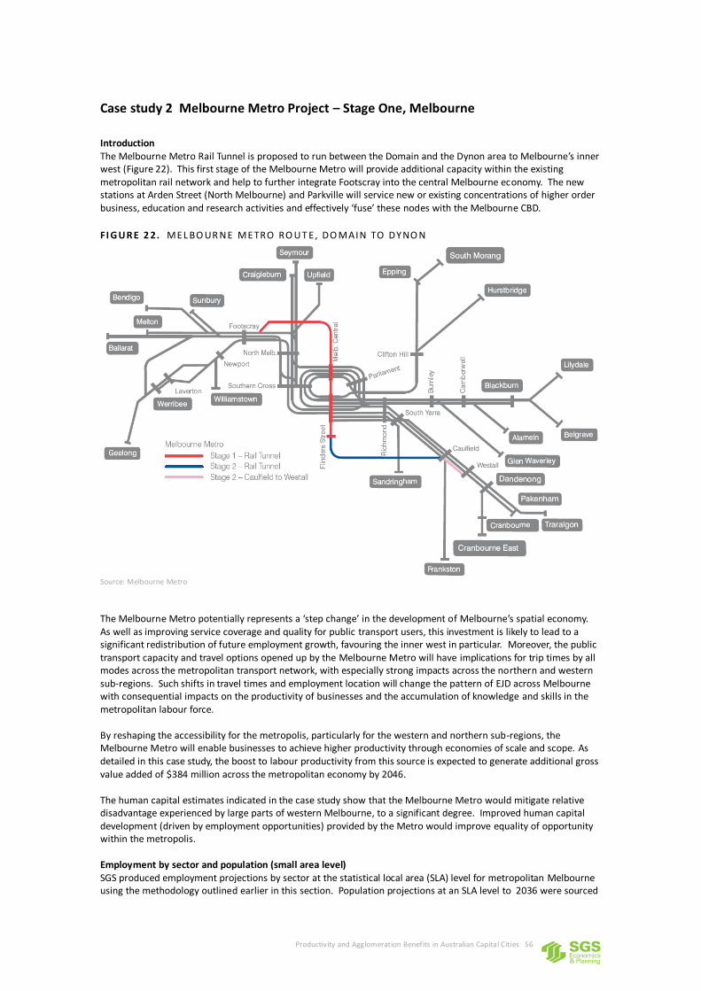
Productivity and Agglomeration Benefits in Australian Capital Cities 56
Case study 2 Melbourne Metro Project – Stage One, Melbourne
Introduction The Melbourne Metro Rail Tunnel is proposed to run between the Domain and the Dynon area to Melbourne’s inner west (Figure 22). This first stage of the Melbourne Metro will provide additional capacity within the existing metropolitan rail network and help to further integrate Footscray into the central Melbourne economy. The new stations at Arden Street (North Melbourne) and Parkville will service new or existing concentrations of higher order business, education and research activities and effectively ‘fuse’ these nodes with the Melbourne CBD.
FI G UR E 2 2. MEL BO UR NE METRO RO U T E, DO MAIN TO DYNO N
Source: Melbourne Metro
The Melbourne Metro potentially represents a ‘step change’ in the development of Melbourne’s spatial economy. As well as improving service coverage and quality for public transport users, this investment is likely to lead to a significant redistribution of future employment growth, favouring the inner west in particular. Moreover, the public transport capacity and travel options opened up by the Melbourne Metro will have implications for trip times by all modes across the metropolitan transport network, with especially strong impacts across the northern and western sub-regions. Such shifts in travel times and employment location will change the pattern of EJD across Melbourne with consequential impacts on the productivity of businesses and the accumulation of knowledge and skills in the metropolitan labour force. By reshaping the accessibility for the metropolis, particularly for the western and northern sub-regions, the Melbourne Metro will enable businesses to achieve higher productivity through economies of scale and scope. As detailed in this case study, the boost to labour productivity from this source is expected to generate additional gross value added of $384 million across the metropolitan economy by 2046. The human capital estimates indicated in the case study show that the Melbourne Metro would mitigate relative disadvantage experienced by large parts of western Melbourne, to a significant degree. Improved human capital development (driven by employment opportunities) provided by the Metro would improve equality of opportunity within the metropolis. Employment by sector and population (small area level) SGS produced employment projections by sector at the statistical local area (SLA) level for metropolitan Melbourne using the methodology outlined earlier in this section. Population projections at an SLA level to 2036 were sourced
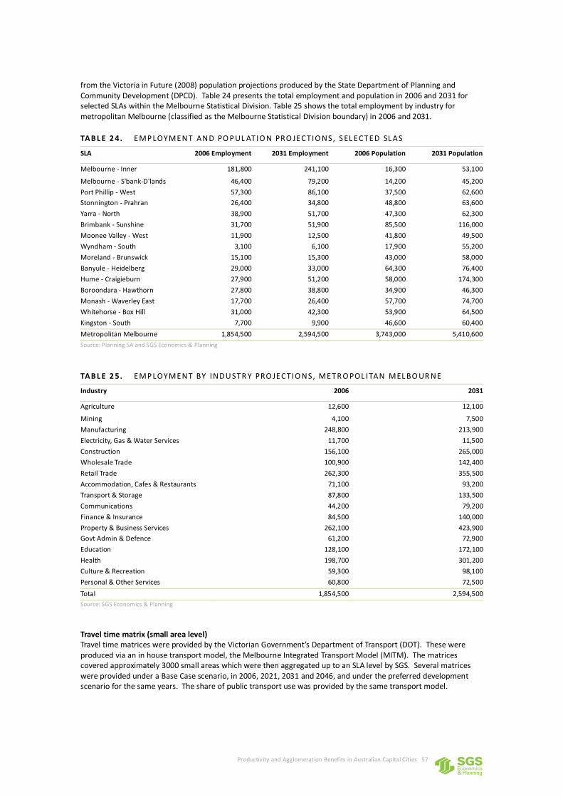
Productivity and Agglomeration Benefits in Australian Capital Cities 57
from the Victoria in Future (2008) population projections produced by the State Department of Planning and Community Development (DPCD). Table 24 presents the total employment and population in 2006 and 2031 for selected SLAs within the Melbourne Statistical Division. Table 25 shows the total employment by industry for metropolitan Melbourne (classified as the Melbourne Statistical Division boundary) in 2006 and 2031.
TAB L E 2 4. EMP LOYMENT AND PO P UL ATIO N PRO JECT IO NS, S EL ECTED SL AS
SLA 2006 Employment 2031 Employment 2006 Population 2031 Population
Melbourne - Inner 181,800 241,100 16,300 53,100
Melbourne - S'bank-D'lands 46,400 79,200 14,200 45,200
Port Phillip - West 57,300 86,100 37,500 62,600
Stonnington - Prahran 26,400 34,800 48,800 63,600
Yarra - North 38,900 51,700 47,300 62,300
Brimbank - Sunshine 31,700 51,900 85,500 116,000
Moonee Valley - West 11,900 12,500 41,800 49,500
Wyndham - South 3,100 6,100 17,900 55,200
Moreland - Brunswick 15,100 15,300 43,000 58,000
Banyule - Heidelberg 29,000 33,000 64,300 76,400
Hume - Craigieburn 27,900 51,200 58,000 174,300
Boroondara - Hawthorn 27,800 38,800 34,900 46,300
Monash - Waverley East 17,700 26,400 57,700 74,700
Whitehorse - Box Hill 31,000 42,300 53,900 64,500
Kingston - South 7,700 9,900 46,600 60,400
Metropolitan Melbourne 1,854,500 2,594,500 3,743,000 5,410,600
Source: Planning SA and SGS Economics & Planning
TAB L E 2 5. EMP LOYMENT BY INDU STR Y PRO JECT IO NS, METR O POL ITAN MEL BO UR NE
Industry 2006 2031
Agriculture 12,600 12,100
Mining 4,100 7,500
Manufacturing 248,800 213,900
Electricity, Gas & Water Services 11,700 11,500
Construction 156,100 265,000
Wholesale Trade 100,900 142,400
Retail Trade 262,300 355,500
Accommodation, Cafes & Restaurants 71,100 93,200
Transport & Storage 87,800 133,500
Communications 44,200 79,200
Finance & Insurance 84,500 140,000
Property & Business Services 262,100 423,900
Govt Admin & Defence 61,200 72,900
Education 128,100 172,100
Health 198,700 301,200
Culture & Recreation 59,300 98,100
Personal & Other Services 60,800 72,500
Total 1,854,500 2,594,500
Source: SGS Economics & Planning
Travel time matrix (small area level) Travel time matrices were provided by the Victorian Government’s Department of Transport (DOT). These were produced via an in house transport model, the Melbourne Integrated Transport Model (MITM). The matrices covered approximately 3000 small areas which were then aggregated up to an SLA level by SGS. Several matrices were provided under a Base Case scenario, in 2006, 2021, 2031 and 2046, and under the preferred development scenario for the same years. The share of public transport use was provided by the same transport model.
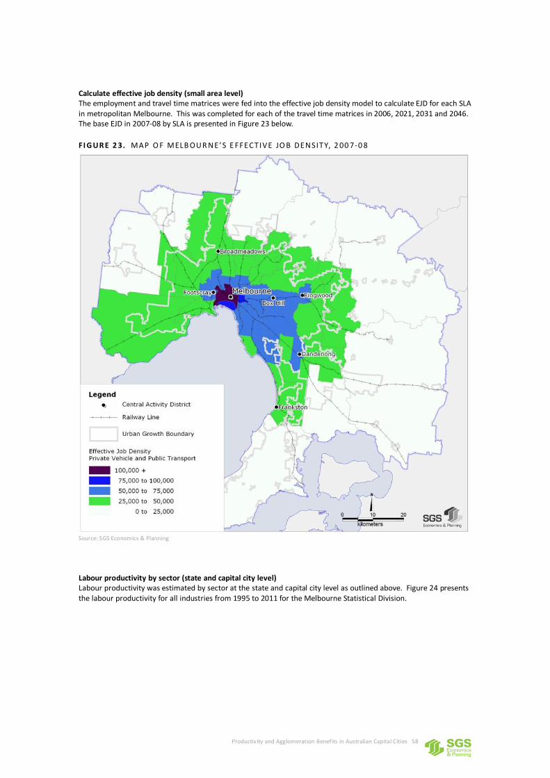
Productivity and Agglomeration Benefits in Australian Capital Cities 58
Calculate effective job density (small area level) The employment and travel time matrices were fed into the effective job density model to calculate EJD for each SLA in metropolitan Melbourne. This was completed for each of the travel time matrices in 2006, 2021, 2031 and 2046. The base EJD in 2007-08 by SLA is presented in Figure 23 below.
FI G UR E 2 3. MAP O F MELB OU R NE’S E FFECTIVE JO B DENSITY, 2 00 7-0 8
Source: SGS Economics & Planning
Labour productivity by sector (state and capital city level) Labour productivity was estimated by sector at the state and capital city level as outlined above. Figure 24 presents the labour productivity for all industries from 1995 to 2011 for the Melbourne Statistical Division.
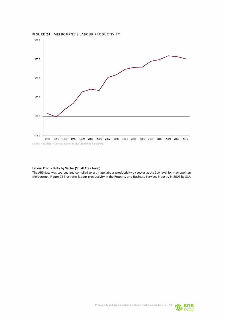
Productivity and Agglomeration Benefits in Australian Capital Cities 59
FI G UR E 2 4. MEL BO UR N E ’S L ABO UR PR O DU CTIV IT Y
Source: ABS State Accounts 5220.0 and SGS Economics & Planning
Labour Productivity by Sector (Small Area Level) The ABS data was sourced and compiled to estimate labour productivity by sector at the SLA level for metropolitan Melbourne. Figure 25 illustrates labour productivity in the Property and Business Services industry in 2006 by SLA.
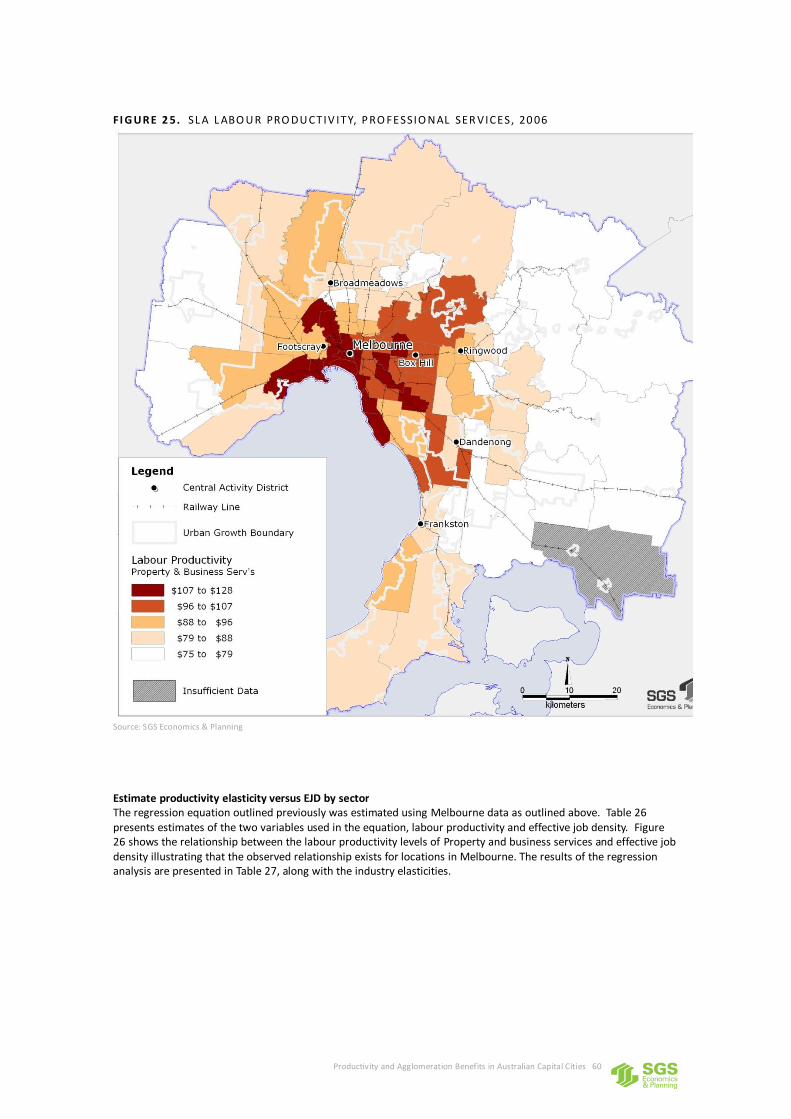
Productivity and Agglomeration Benefits in Australian Capital Cities 60
FI G UR E 2 5. SL A L ABO U R PRO DU CTIV ITY, P RO FESSIO NAL SER VICES, 20 06
Source: SGS Economics & Planning
Estimate productivity elasticity versus EJD by sector The regression equation outlined previously was estimated using Melbourne data as outlined above. Table 26 presents estimates of the two variables used in the equation, labour productivity and effective job density. Figure 26 shows the relationship between the labour productivity levels of Property and business services and effective job density illustrating that the observed relationship exists for locations in Melbourne. The results of the regression analysis are presented in Table 27, along with the industry elasticities.
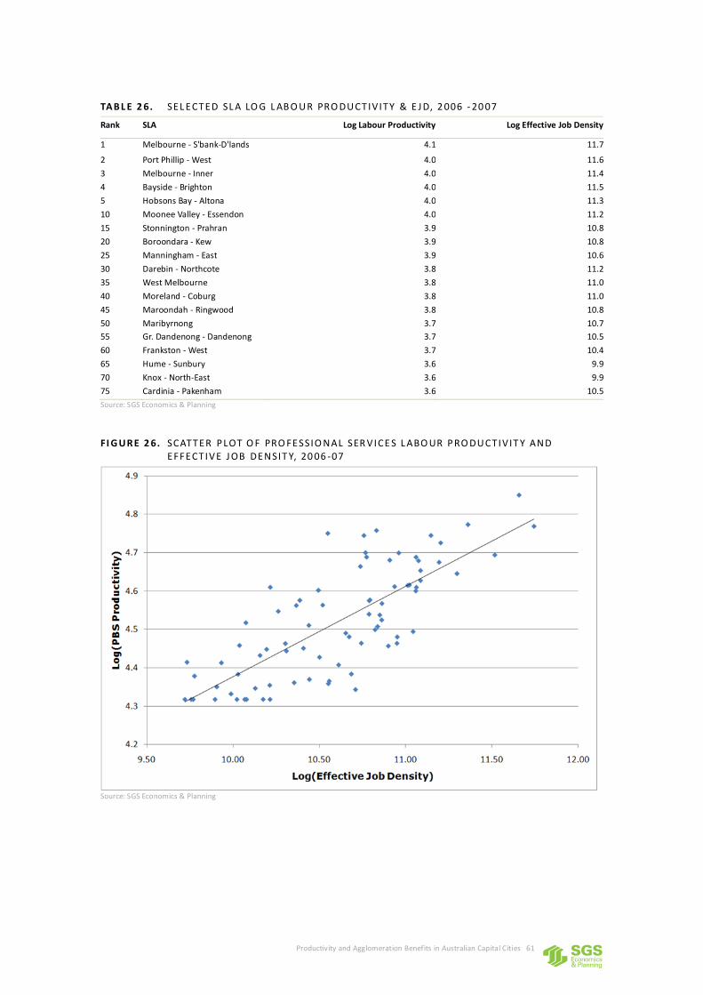
Productivity and Agglomeration Benefits in Australian Capital Cities 61
TAB L E 2 6. SEL ECTED SL A LO G L AB O U R PRO DU CTIV ITY & E J D, 2 006 - 20 07
Rank SLA Log Labour Productivity Log Effective Job Density
1 Melbourne - S'bank-D'lands 4.1 11.7
2 Port Phillip - West 4.0 11.6
3 Melbourne - Inner 4.0 11.4
4 Bayside - Brighton 4.0 11.5
5 Hobsons Bay - Altona 4.0 11.3
10 Moonee Valley - Essendon 4.0 11.2
15 Stonnington - Prahran 3.9 10.8
20 Boroondara - Kew 3.9 10.8
25 Manningham - East 3.9 10.6
30 Darebin - Northcote 3.8 11.2
35 West Melbourne 3.8 11.0
40 Moreland - Coburg 3.8 11.0
45 Maroondah - Ringwood 3.8 10.8
50 Maribyrnong 3.7 10.7
55 Gr. Dandenong - Dandenong 3.7 10.5
60 Frankston - West 3.7 10.4
65 Hume - Sunbury 3.6 9.9
70 Knox - North-East 3.6 9.9
75 Cardinia - Pakenham 3.6 10.5
Source: SGS Economics & Planning
F I G UR E 2 6. SCATTER P LOT O F PRO FESSIO NAL SER VICE S L ABO UR P RO DU CTIV IT Y AND EFFECTIVE J OB DENSIT Y, 20 06 -07
Source: SGS Economics & Planning
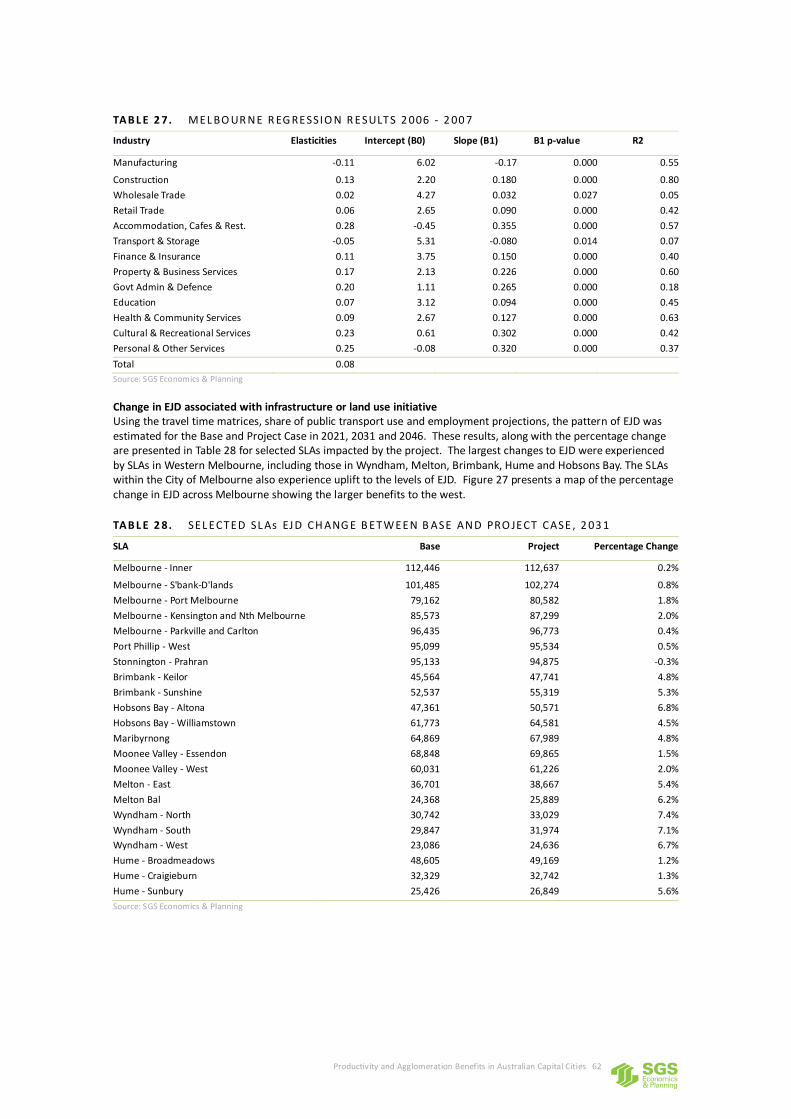
Productivity and Agglomeration Benefits in Australian Capital Cities 62
TAB L E 2 7. MEL BO UR NE R EG RESSIO N R ESULTS 2 006 - 2 00 7
Industry Elasticities Intercept (B0) Slope (B1) B1 p-value R2
Manufacturing -0.11 6.02 -0.17 0.000 0.55
Construction 0.13 2.20 0.180 0.000 0.80
Wholesale Trade 0.02 4.27 0.032 0.027 0.05
Retail Trade 0.06 2.65 0.090 0.000 0.42
Accommodation, Cafes & Rest. 0.28 -0.45 0.355 0.000 0.57
Transport & Storage -0.05 5.31 -0.080 0.014 0.07
Finance & Insurance 0.11 3.75 0.150 0.000 0.40
Property & Business Services 0.17 2.13 0.226 0.000 0.60
Govt Admin & Defence 0.20 1.11 0.265 0.000 0.18
Education 0.07 3.12 0.094 0.000 0.45
Health & Community Services 0.09 2.67 0.127 0.000 0.63
Cultural & Recreational Services 0.23 0.61 0.302 0.000 0.42
Personal & Other Services 0.25 -0.08 0.320 0.000 0.37
Total 0.08
Source: SGS Economics & Planning
Change in EJD associated with infrastructure or land use initiative Using the travel time matrices, share of public transport use and employment projections, the pattern of EJD was estimated for the Base and Project Case in 2021, 2031 and 2046. These results, along with the percentage change are presented in Table 28 for selected SLAs impacted by the project. The largest changes to EJD were experienced by SLAs in Western Melbourne, including those in Wyndham, Melton, Brimbank, Hume and Hobsons Bay. The SLAs within the City of Melbourne also experience uplift to the levels of EJD. Figure 27 presents a map of the percentage change in EJD across Melbourne showing the larger benefits to the west.
TAB L E 2 8. SEL ECTED SL As EJ D CH ANG E B ETWEEN B ASE AND PRO JECT CASE , 2 03 1
SLA Base Project Percentage Change
Melbourne - Inner 112,446 112,637 0.2%
Melbourne - S'bank-D'lands 101,485 102,274 0.8%
Melbourne - Port Melbourne 79,162 80,582 1.8%
Melbourne - Kensington and Nth Melbourne 85,573 87,299 2.0%
Melbourne - Parkville and Carlton 96,435 96,773 0.4%
Port Phillip - West 95,099 95,534 0.5%
Stonnington - Prahran 95,133 94,875 -0.3%
Brimbank - Keilor 45,564 47,741 4.8%
Brimbank - Sunshine 52,537 55,319 5.3%
Hobsons Bay - Altona 47,361 50,571 6.8%
Hobsons Bay - Williamstown 61,773 64,581 4.5%
Maribyrnong 64,869 67,989 4.8%
Moonee Valley - Essendon 68,848 69,865 1.5%
Moonee Valley - West 60,031 61,226 2.0%
Melton - East 36,701 38,667 5.4%
Melton Bal 24,368 25,889 6.2%
Wyndham - North 30,742 33,029 7.4%
Wyndham - South 29,847 31,974 7.1%
Wyndham - West 23,086 24,636 6.7%
Hume - Broadmeadows 48,605 49,169 1.2%
Hume - Craigieburn 32,329 32,742 1.3%
Hume - Sunbury 25,426 26,849 5.6%
Source: SGS Economics & Planning
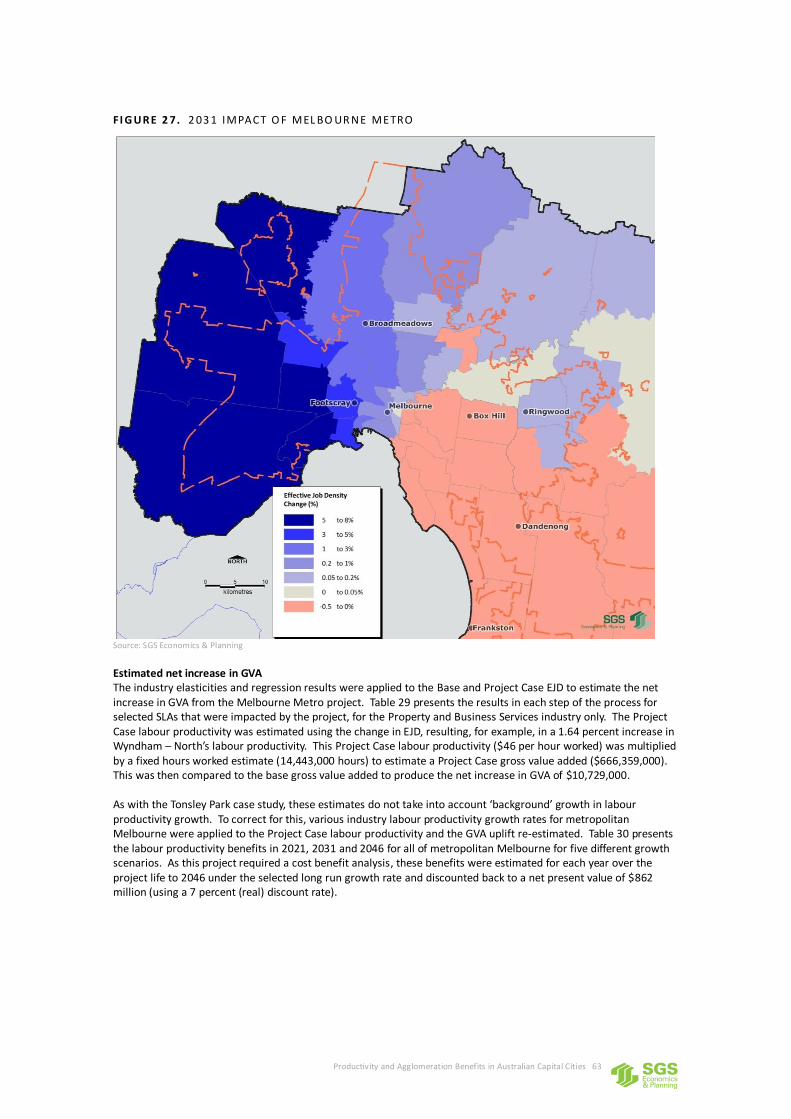
Productivity and Agglomeration Benefits in Australian Capital Cities 63
FI G UR E 2 7. 2 03 1 IMPACT O F MEL BO UR NE METRO
Source: SGS Economics & Planning
Estimated net increase in GVA The industry elasticities and regression results were applied to the Base and Project Case EJD to estimate the net increase in GVA from the Melbourne Metro project. Table 29 presents the results in each step of the process for selected SLAs that were impacted by the project, for the Property and Business Services industry only. The Project Case labour productivity was estimated using the change in EJD, resulting, for example, in a 1.64 percent increase in Wyndham – North’s labour productivity. This Project Case labour productivity ($46 per hour worked) was multiplied by a fixed hours worked estimate (14,443,000 hours) to estimate a Project Case gross value added ($666,359,000). This was then compared to the base gross value added to produce the net increase in GVA of $10,729,000. As with the Tonsley Park case study, these estimates do not take into account ‘background’ growth in labour productivity growth. To correct for this, various industry labour productivity growth rates for metropolitan Melbourne were applied to the Project Case labour productivity and the GVA uplift re-estimated. Table 30 presents the labour productivity benefits in 2021, 2031 and 2046 for all of metropolitan Melbourne for five different growth scenarios. As this project required a cost benefit analysis, these benefits were estimated for each year over the project life to 2046 under the selected long run growth rate and discounted back to a net present value of $862 million (using a 7 percent (real) discount rate).
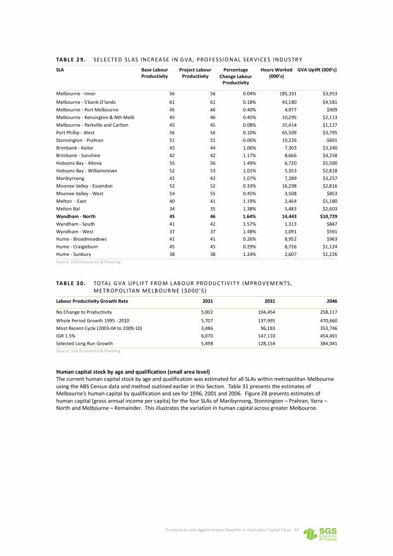
Productivity and Agglomeration Benefits in Australian Capital Cities 64
TAB L E 2 9. SEL ECTED SL AS INCR EA SE IN G VA, PRO FESSIO NAL SER VICES INDU STR Y
SLA Base Labour Productivity
Project Labour Productivity
Percentage
Change Labour Productivity
Hours Worked (000’s)
GVA Uplift (000’s)
Melbourne - Inner 56 56 0.04% 185,331 $3,953
Melbourne - S'bank-D'lands 61 61 0.18% 43,180 $4,581
Melbourne - Port Melbourne 45 46 0.40% 4,977 $909
Melbourne - Kensington & Nth Melb 45 46 0.45% 10,295 $2,113
Melbourne - Parkville and Carlton 45 45 0.08% 31,414 $1,127
Port Phillip - West 56 56 0.10% 65,509 $3,795
Stonnington - Prahran 51 51 -0.06% 19,226 -$601
Brimbank - Keilor 43 44 1.06% 7,303 $3,340
Brimbank - Sunshine 42 42 1.17% 8,666 $4,258
Hobsons Bay - Altona 55 56 1.49% 6,720 $5,500
Hobsons Bay - Williamstown 52 53 1.01% 5,353 $2,818
Maribyrnong 42 42 1.07% 7,289 $3,257
Moonee Valley - Essendon 52 52 0.33% 16,298 $2,816
Moonee Valley - West 54 55 0.45% 3,508 $853
Melton - East 40 41 1.19% 2,464 $1,180
Melton Bal 34 35 1.38% 5,483 $2,603
Wyndham - North 45 46 1.64% 14,443 $10,729
Wyndham - South 41 42 1.57% 1,313 $847
Wyndham - West 37 37 1.48% 1,091 $591
Hume - Broadmeadows 41 41 0.26% 8,952 $963
Hume - Craigieburn 45 45 0.29% 8,726 $1,124
Hume - Sunbury 38 38 1.24% 2,607 $1,226
Source: SGS Economics & Planning
TAB L E 3 0. TOTAL G VA UP L IFT FRO M L AB O UR PRO DU CTIV IT Y IMPRO VEMENTS, METR OP OL ITAN MELB OU R N E ( $0 00 ’S)
Labour Productivity Growth Rate 2021 2031 2046
No Change to Productivity 5,002 104,454 258,117
Whole Period Growth 1995 - 2010 5,707 137,995 470,660
Most Recent Cycle (2003-04 to 2009-10) 3,486 96,183 353,746
IGR 1.5% 6,070 147,110 454,491
Selected Long Run Growth 5,498 128,154 384,041
Source: SGS Economics & Planning
Human capital stock by age and qualification (small area level) The current human capital stock by age and qualification was estimated for all SLAs within metropolitan Melbourne using the ABS Census data and method outlined earlier in this Section. Table 31 presents the estimates of Melbourne’s human capital by qualification and sex for 1996, 2001 and 2006. Figure 28 presents estimates of human capital (gross annual income per capita) for the four SLAs of Maribyrnong, Stonnington – Prahran, Yarra – North and Melbourne – Remainder. This illustrates the variation in human capital across greater Melbourne.
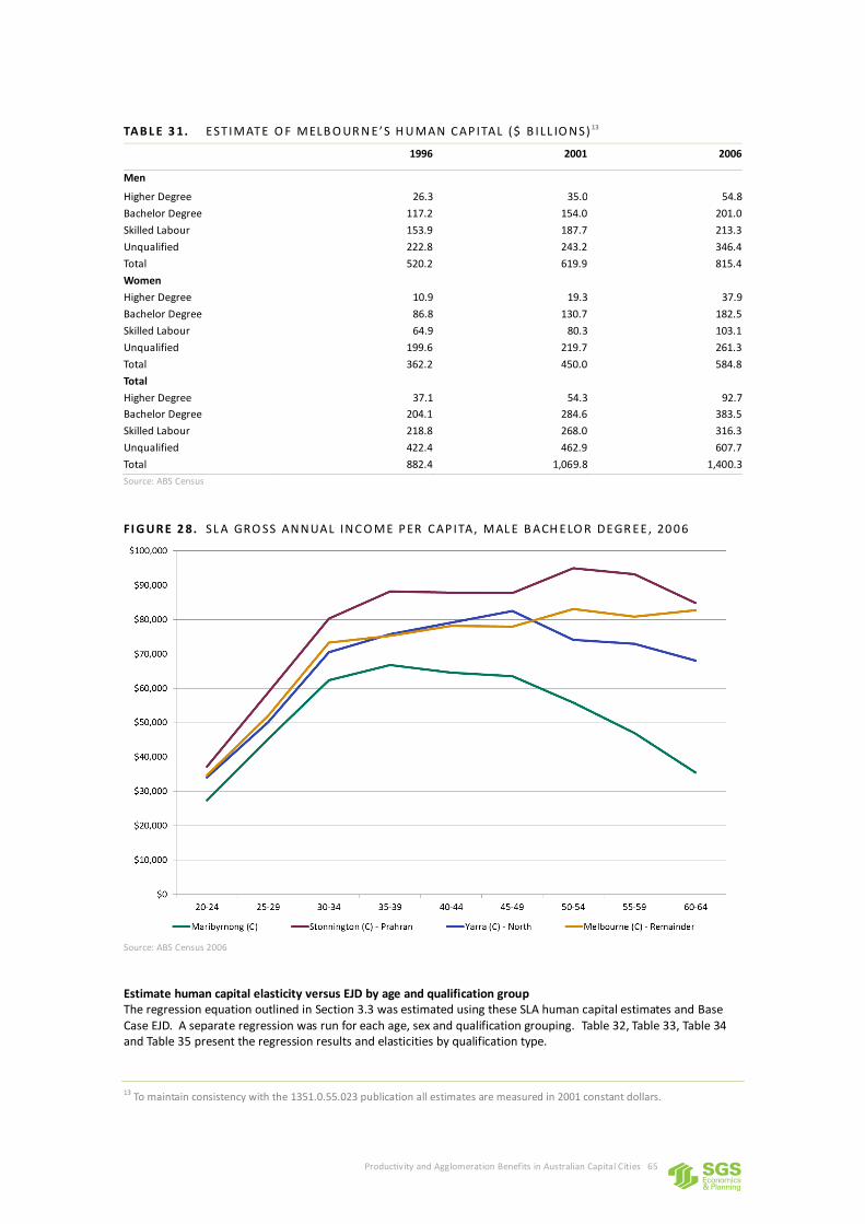
Productivity and Agglomeration Benefits in Australian Capital Cities 65
TAB L E 3 1. EST IMATE O F MELB O UR N E ’S H U MAN CAP ITAL ($ B ILL IO NS) 13
1996 2001 2006
Men
Higher Degree 26.3 35.0 54.8
Bachelor Degree 117.2 154.0 201.0
Skilled Labour 153.9 187.7 213.3
Unqualified 222.8 243.2 346.4
Total 520.2 619.9 815.4
Women
Higher Degree 10.9 19.3 37.9
Bachelor Degree 86.8 130.7 182.5
Skilled Labour 64.9 80.3 103.1
Unqualified 199.6 219.7 261.3
Total 362.2 450.0 584.8
Total
Higher Degree 37.1 54.3 92.7
Bachelor Degree 204.1 284.6 383.5
Skilled Labour 218.8 268.0 316.3
Unqualified 422.4 462.9 607.7
Total 882.4 1,069.8 1,400.3
Source: ABS Census
F I G UR E 2 8. SL A GRO SS ANNUAL INC O ME P ER CAP ITA, MAL E B ACH ELO R DEGR EE, 20 0 6
Source: ABS Census 2006
Estimate human capital elasticity versus EJD by age and qualification group The regression equation outlined in Section 3.3 was estimated using these SLA human capital estimates and Base Case EJD. A separate regression was run for each age, sex and qualification grouping. Table 32, Table 33, Table 34 and Table 35 present the regression results and elasticities by qualification type.
13 To maintain consistency with the 1351.0.55.023 publication all estimates are measured in 2001 constant dollars.

Productivity and Agglomeration Benefits in Australian Capital Cities 66
TAB L E 3 2. U NQ UAL IFIED R EGR ESSI O N R ESU LTS
Elasticity Intercept (B0) Slope (B1) B1 p-value SEIFA (B2) B2 p-value R-Squared
Male
20-24 0.093 7.21 0.13 0.00 0.05 0.00 0.694
25-29 0.100 7.00 0.14 0.00 0.05 0.00 0.701
30-34 0.096 6.93 0.13 0.00 0.06 0.00 0.708
35-39 0.086 6.91 0.12 0.00 0.06 0.00 0.727
40-44 0.071 6.90 0.10 0.00 0.06 0.00 0.724
45-49 0.064 6.75 0.09 0.01 0.06 0.00 0.721
50-54 0.070 6.33 0.10 0.01 0.06 0.00 0.710
55-59 0.080 5.69 0.11 0.00 0.06 0.00 0.679
60-64 0.075 4.92 0.10 0.02 0.07 0.00 0.640
Female
20-24 0.229 5.08 0.30 0.00 0.03 0.00 0.621
25-29 0.229 4.95 0.30 0.00 0.04 0.00 0.601
30-34 0.206 5.09 0.27 0.00 0.04 0.00 0.572
35-39 0.166 5.43 0.22 0.00 0.04 0.00 0.577
40-44 0.144 5.51 0.19 0.00 0.04 0.00 0.613
45-49 0.135 5.36 0.18 0.00 0.05 0.00 0.627
50-54 0.141 4.93 0.19 0.00 0.05 0.00 0.628
55-59 0.153 4.25 0.21 0.00 0.06 0.00 0.614
60-64 0.151 3.45 0.20 0.00 0.06 0.00 0.588
Source: SGS Economics & Planning
TAB L E 3 3. SK IL L ED L ABO U R R EGR E SSIO N R ESU LTS
Elasticity Intercept (B0) Slope (B1) B1 p-value SEIFA (B2) B2 p-value R-Squared
Male
20-24 0.074 7.75 0.10 0.00 0.03 0.00 0.660
25-29 0.089 7.45 0.12 0.00 0.04 0.00 0.677
30-34 0.099 7.19 0.14 0.00 0.04 0.00 0.690
35-39 0.100 7.02 0.14 0.00 0.04 0.00 0.701
40-44 0.097 6.85 0.13 0.00 0.04 0.00 0.711
45-49 0.099 6.57 0.14 0.00 0.04 0.00 0.717
50-54 0.107 6.14 0.15 0.00 0.04 0.00 0.714
55-59 0.128 5.37 0.17 0.00 0.04 0.00 0.703
60-64 0.146 4.32 0.20 0.00 0.05 0.00 0.677
Female
20-24 0.177 5.99 0.23 0.00 0.02 0.00 0.593
25-29 0.207 5.50 0.27 0.00 0.02 0.00 0.615
30-34 0.203 5.41 0.27 0.00 0.02 0.00 0.575
35-39 0.167 5.72 0.22 0.00 0.02 0.00 0.528
40-44 0.148 5.78 0.20 0.00 0.02 0.00 0.535
45-49 0.144 5.59 0.19 0.00 0.03 0.00 0.549
50-54 0.150 5.17 0.20 0.00 0.03 0.00 0.569
55-59 0.171 4.43 0.23 0.00 0.03 0.00 0.533
60-64 0.190 3.37 0.25 0.00 0.04 0.00 0.436
Source: SGS Economics & Planning
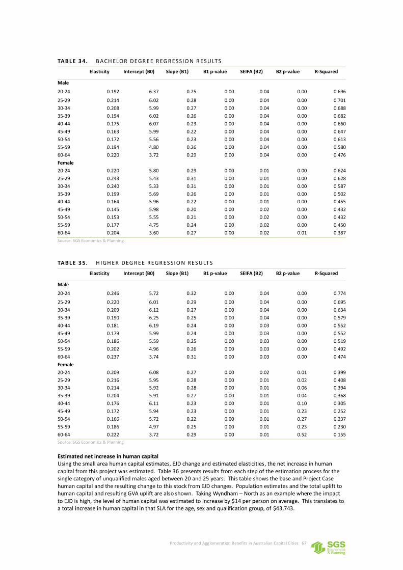
Productivity and Agglomeration Benefits in Australian Capital Cities 67
TAB L E 3 4. B ACH ELOR DEGR EE R EG R ESSIO N R ESULTS
Elasticity Intercept (B0) Slope (B1) B1 p-value SEIFA (B2) B2 p-value R-Squared
Male
20-24 0.192 6.37 0.25 0.00 0.04 0.00 0.696
25-29 0.214 6.02 0.28 0.00 0.04 0.00 0.701
30-34 0.208 5.99 0.27 0.00 0.04 0.00 0.688
35-39 0.194 6.02 0.26 0.00 0.04 0.00 0.682
40-44 0.175 6.07 0.23 0.00 0.04 0.00 0.660
45-49 0.163 5.99 0.22 0.00 0.04 0.00 0.647
50-54 0.172 5.56 0.23 0.00 0.04 0.00 0.613
55-59 0.194 4.80 0.26 0.00 0.04 0.00 0.580
60-64 0.220 3.72 0.29 0.00 0.04 0.00 0.476
Female
20-24 0.220 5.80 0.29 0.00 0.01 0.00 0.624
25-29 0.243 5.43 0.31 0.00 0.01 0.00 0.628
30-34 0.240 5.33 0.31 0.00 0.01 0.00 0.587
35-39 0.199 5.69 0.26 0.00 0.01 0.00 0.502
40-44 0.164 5.96 0.22 0.00 0.01 0.00 0.455
45-49 0.145 5.98 0.20 0.00 0.02 0.00 0.432
50-54 0.153 5.55 0.21 0.00 0.02 0.00 0.432
55-59 0.177 4.75 0.24 0.00 0.02 0.00 0.450
60-64 0.204 3.60 0.27 0.00 0.02 0.01 0.387
Source: SGS Economics & Planning
TAB L E 3 5. H IGH ER DEG R EE REGR ES SIO N RESU LTS
Elasticity Intercept (B0) Slope (B1) B1 p-value SEIFA (B2) B2 p-value R-Squared
Male
20-24 0.246 5.72 0.32 0.00 0.04 0.00 0.774
25-29 0.220 6.01 0.29 0.00 0.04 0.00 0.695
30-34 0.209 6.12 0.27 0.00 0.04 0.00 0.634
35-39 0.190 6.25 0.25 0.00 0.04 0.00 0.579
40-44 0.181 6.19 0.24 0.00 0.03 0.00 0.552
45-49 0.179 5.99 0.24 0.00 0.03 0.00 0.552
50-54 0.186 5.59 0.25 0.00 0.03 0.00 0.519
55-59 0.202 4.96 0.26 0.00 0.03 0.00 0.492
60-64 0.237 3.74 0.31 0.00 0.03 0.00 0.474
Female
20-24 0.209 6.08 0.27 0.00 0.02 0.01 0.399
25-29 0.216 5.95 0.28 0.00 0.01 0.02 0.408
30-34 0.214 5.92 0.28 0.00 0.01 0.06 0.394
35-39 0.204 5.91 0.27 0.00 0.01 0.04 0.368
40-44 0.176 6.11 0.23 0.00 0.01 0.10 0.305
45-49 0.172 5.94 0.23 0.00 0.01 0.23 0.252
50-54 0.166 5.72 0.22 0.00 0.01 0.27 0.237
55-59 0.186 4.97 0.25 0.00 0.01 0.23 0.230
60-64 0.222 3.72 0.29 0.00 0.01 0.52 0.155
Source: SGS Economics & Planning
Estimated net increase in human capital Using the small area human capital estimates, EJD change and estimated elasticities, the net increase in human capital from this project was estimated. Table 36 presents results from each step of the estimation process for the single category of unqualified males aged between 20 and 25 years. This table shows the base and Project Case human capital and the resulting change to this stock from EJD changes. Population estimates and the total uplift to human capital and resulting GVA uplift are also shown. Taking Wyndham – North as an example where the impact to EJD is high, the level of human capital was estimated to increase by $14 per person on average. This translates to a total increase in human capital in that SLA for the age, sex and qualification group, of $43,743.
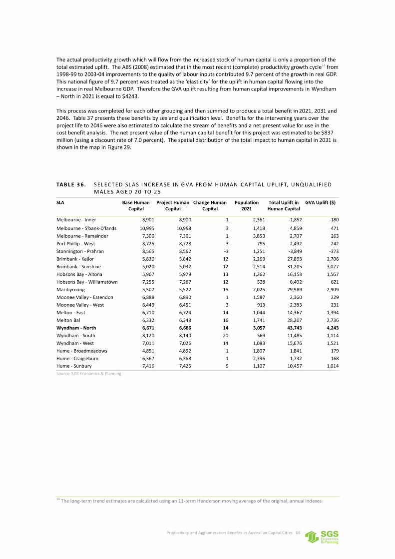
Productivity and Agglomeration Benefits in Australian Capital Cities 68
The actual productivity growth which will flow from the increased stock of human capital is only a proportion of the total estimated uplift. The ABS (2008) estimated that in the most recent (complete) productivity growth cycle14 from 1998-99 to 2003-04 improvements to the quality of labour inputs contributed 9.7 percent of the growth in real GDP. This national figure of 9.7 percent was treated as the ‘elasticity’ for the uplift in human capital flowing into the increase in real Melbourne GDP. Therefore the GVA uplift resulting from human capital improvements in Wyndham – North in 2021 is equal to $4243. This process was completed for each other grouping and then summed to produce a total benefit in 2021, 2031 and 2046. Table 37 presents these benefits by sex and qualification level. Benefits for the intervening years over the project life to 2046 were also estimated to calculate the stream of benefits and a net present value for use in the cost benefit analysis. The net present value of the human capital benefit for this project was estimated to be $837 million (using a discount rate of 7.0 percent). The spatial distribution of the total impact to human capital in 2031 is shown in the map in Figure 29.
TAB L E 3 6. SEL ECTED SL AS INCR EA SE IN G VA FR O M H U MAN CAP ITAL U PL IFT, U NQ UAL IFIED MAL ES AG ED 20 TO 25
SLA Base Human Capital
Project Human Capital
Change Human Capital
Population 2021
Total Uplift in Human Capital
GVA Uplift ($)
Melbourne - Inner 8,901 8,900 -1 2,361 -1,852 -180
Melbourne - S'bank-D'lands 10,995 10,998 3 1,418 4,859 471
Melbourne - Remainder 7,300 7,301 1 3,853 2,707 263
Port Phillip - West 8,725 8,728 3 795 2,492 242
Stonnington - Prahran 8,565 8,562 -3 1,251 -3,849 -373
Brimbank - Keilor 5,830 5,842 12 2,269 27,893 2,706
Brimbank - Sunshine 5,020 5,032 12 2,514 31,205 3,027
Hobsons Bay - Altona 5,967 5,979 13 1,262 16,153 1,567
Hobsons Bay - Williamstown 7,255 7,267 12 528 6,402 621
Maribyrnong 5,507 5,522 15 2,025 29,989 2,909
Moonee Valley - Essendon 6,888 6,890 1 1,587 2,360 229
Moonee Valley - West 6,449 6,451 3 913 2,383 231
Melton - East 6,710 6,724 14 1,044 14,367 1,394
Melton Bal 6,332 6,348 16 1,741 28,207 2,736
Wyndham - North 6,671 6,686 14 3,057 43,743 4,243
Wyndham - South 8,120 8,140 20 569 11,485 1,114
Wyndham - West 7,011 7,026 14 1,083 15,676 1,521
Hume - Broadmeadows 4,851 4,852 1 1,807 1,841 179
Hume - Craigieburn 6,367 6,368 1 2,396 1,732 168
Hume - Sunbury 7,416 7,425 9 1,107 10,457 1,014
Source: SGS Economics & Planning
14 The long-term trend estimates are calculated using an 11-term Henderson moving average of the original, annual indexes
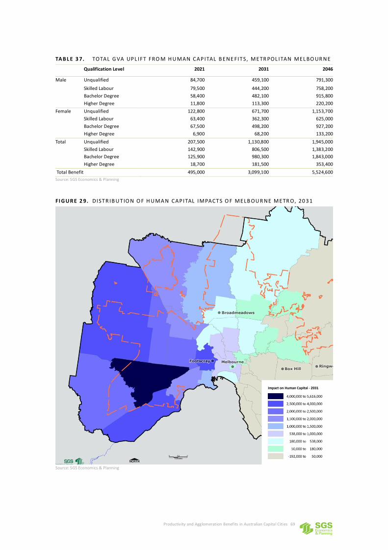
Productivity and Agglomeration Benefits in Australian Capital Cities 69
TAB L E 3 7. TOTAL G VA UP L IFT FRO M H U MAN CAP ITAL B ENE FITS, METR POL ITAN MEL BO UR NE
Qualification Level 2021 2031 2046
Male Unqualified 84,700 459,100 791,300
Skilled Labour 79,500 444,200 758,200
Bachelor Degree 58,400 482,100 915,800
Higher Degree 11,800 113,300 220,200
Female Unqualified 122,800 671,700 1,153,700
Skilled Labour 63,400 362,300 625,000
Bachelor Degree 67,500 498,200 927,200
Higher Degree 6,900 68,200 133,200
Total Unqualified 207,500 1,130,800 1,945,000
Skilled Labour 142,900 806,500 1,383,200
Bachelor Degree 125,900 980,300 1,843,000
Higher Degree 18,700 181,500 353,400
Total Benefit 495,000 3,099,100 5,524,600
Source: SGS Economics & Planning
FI G UR E 2 9. DISTR IB U TIO N O F H U MA N CAP ITAL IMPACTS O F MELB OU R NE METR O, 20 3 1
Source: SGS Economics & Planning
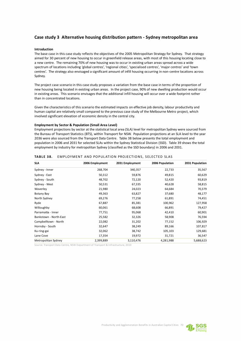
Productivity and Agglomeration Benefits in Australian Capital Cities 70
Case study 3 Alternative housing distribution pattern - Sydney metropolitan area
Introduction The base case in this case study reflects the objectives of the 2005 Metropolitan Strategy for Sydney. That strategy aimed for 30 percent of new housing to occur in greenfield release areas, with most of this housing locating close to a new centre. The remaining 70% of new housing was to occur in existing urban areas spread across a wide spectrum of locations including ‘global centres’, ‘regional cities’, ‘specialised centres’, ‘major centres’ and ‘town centres’. The strategy also envisaged a significant amount of infill housing occurring in non-centre locations across Sydney. The project case scenario in this case study proposes a variation from the base case in terms of the proportion of new housing being located in existing urban areas. In the project case, 90% of new dwelling production would occur in existing areas. This scenario envisages that the additional infill housing will occur over a wide footprint rather than in concentrated locations. Given the characteristics of this scenario the estimated impacts on effective job density, labour productivity and human capital are relatively small compared to the previous case study of the Melbourne Metro project, which involved significant elevation of economic density in the central city. Employment by Sector & Population (Small Area Level) Employment projections by sector at the statistical local area (SLA) level for metropolitan Sydney were sourced from the Bureau of Transport Statistics (BTS), within Transport for NSW. Population projections at an SLA level to the year 2036 were also sourced from the Transport Data Centre. Table 38 below presents the total employment and population in 2006 and 2031 for selected SLAs within the Sydney Statistical Division (SSD). Table 39 shows the total employment by industry for metropolitan Sydney (classified as the SSD boundary) in 2006 and 2031.
TAB L E 3 8. EMP LOYMENT AND PO P UL ATIO N PRO JECT IO NS, S EL ECTED SL AS
SLA 2006 Employment 2031 Employment 2006 Population 2031 Population
Sydney - Inner 268,704 340,357 22,733 35,567
Sydney - East 50,312 59,876 49,815 60,629
Sydney - South 48,702 72,120 52,420 93,819
Sydney - West 50,531 67,335 40,628 58,815
Waverley 21,980 24,023 64,684 70,379
Botany Bay 49,363 63,827 37,680 48,177
North Sydney 69,276 77,258 61,891 74,451
Ryde 67,887 85,381 100,962 127,958
Willoughby 60,061 68,608 66,891 79,427
Parramatta - Inner 77,751 95,068 42,410 60,901
Bankstown - North-East 25,582 32,326 58,908 76,594
Campbelltown - North 22,082 31,202 77,152 106,929
Hornsby - South 32,647 38,249 89,166 107,817
Ku-ring-gai 32,062 38,742 105,103 129,681
Lane Cove 17,354 19,972 31,721 36,547
Metropolitan Sydney 2,399,889 3,110,476 4,281,988 5,688,623
Source: Transport Data Centre, NSW Department of Transport & Infrastructure, 2010

Productivity and Agglomeration Benefits in Australian Capital Cities 71
TAB L E 3 9. EMP LOYMENT BY INDU STR Y PRO JECT IO NS, METR O POL ITAN SYDNEY
Industry 2006 2031
Agriculture, Forestry & Fishing 8,689 11,121
Mining 4,505 5,266
Manufacturing 208,618 232,765
Electricity, Gas, Water & Waste 17,755 17,630
Construction 116,719 132,555
Wholesale Trade 119,186 122,481
Retail Trade 225,235 335,405
Accommodation & Food Services 128,609 201,628
Transport, Postal & Warehousing 111,952 144,940
Information Media & Telecom 63,096 62,973
Financial & Insurance Services 138,894 163,610
Rental, Hiring & Real Estate Services 39,683 59,850
Professional, Scientific & Technical Services 189,516 259,001
Administrative & Support Services 66,749 68,005
Public Administration & Safety 120,636 159,000
Education & Training 154,129 216,131
Health Care & Social Assistance 211,282 309,083
Arts & Recreation Services 30,188 37,598
Other Services 77,752 109,864
Total 2,033,190 2,648,907
Source: Transport Data Centre, NSW Department of Transport & Infrastructure, 2010
Travel time matrix (small area level) Travel time matrices were also provided by the BTS. These were produced by the BTS in-house via the Strategic Transport Model (STM). The matrices covered approximately 2700 small areas which were then aggregated up to an SLA level by SGS. Four matrices were provided covering the base case and project case scenarios in 2031 for car and public transport use. The share of public transport use was sourced from the ABS 2006 Census.
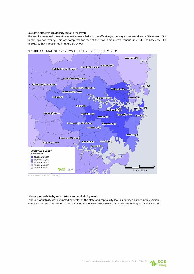
Productivity and Agglomeration Benefits in Australian Capital Cities 72
Calculate effective job density (small area level) The employment and travel time matrices were fed into the effective job density model to calculate EJD for each SLA in metropolitan Sydney. This was completed for each of the travel time matrix scenarios in 2031. The base case EJD in 2031 by SLA is presented in Figure 30 below.
FI G UR E 3 0. MAP O F SYDNEY’S EFFECT IVE JO B DENSITY, 2 03 1
Source: SGS Economics & Planning
Labour productivity by sector (state and capital city level) Labour productivity was estimated by sector at the state and capital city level as outlined earlier in this section. Figure 31 presents the labour productivity for all industries from 1995 to 2011 for the Sydney Statistical Division.
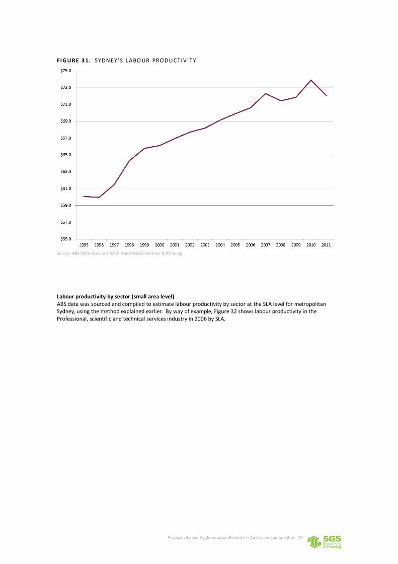
Productivity and Agglomeration Benefits in Australian Capital Cities 73
FI G UR E 3 1. SYDNEY ’ S L ABO UR PRO DU CTIV ITY
Source: ABS State Accounts 5220.0 and SGS Economics & Planning
Labour productivity by sector (small area level) ABS data was sourced and compiled to estimate labour productivity by sector at the SLA level for metropolitan Sydney, using the method explained earlier. By way of example, Figure 32 shows labour productivity in the Professional, scientific and technical services industry in 2006 by SLA.
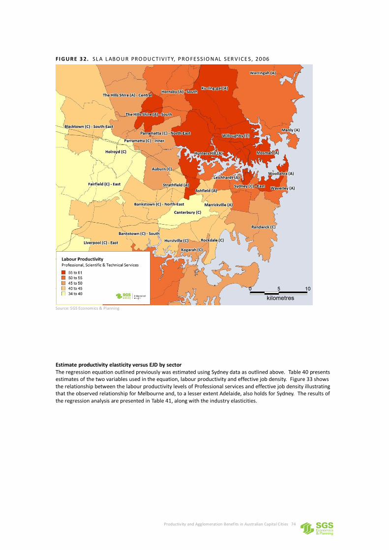
Productivity and Agglomeration Benefits in Australian Capital Cities 74
FI G UR E 3 2. SL A L ABO U R PRO DU CTIV ITY, P RO FESSIO NAL SER VICE S, 20 06
Source: SGS Economics & Planning
Estimate productivity elasticity versus EJD by sector The regression equation outlined previously was estimated using Sydney data as outlined above. Table 40 presents estimates of the two variables used in the equation, labour productivity and effective job density. Figure 33 shows the relationship between the labour productivity levels of Professional services and effective job density illustrating that the observed relationship for Melbourne and, to a lesser extent Adelaide, also holds for Sydney. The results of the regression analysis are presented in Table 41, along with the industry elasticities.
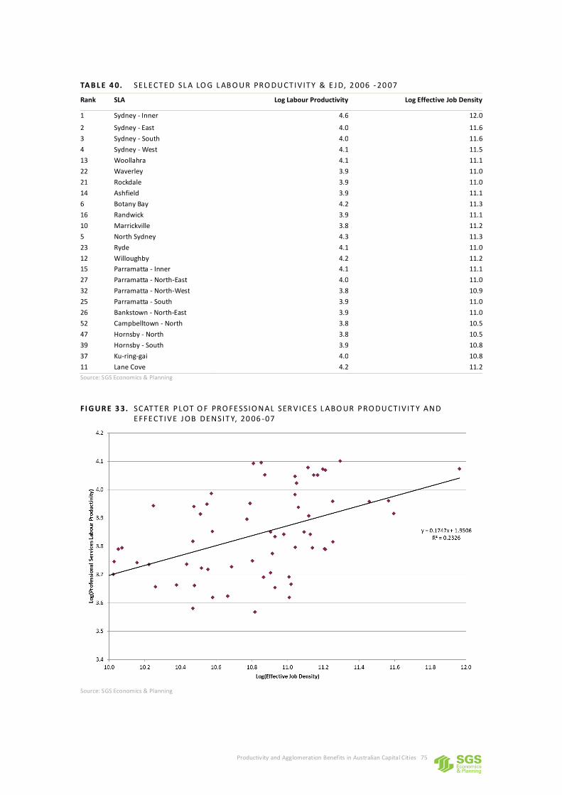
Productivity and Agglomeration Benefits in Australian Capital Cities 75
TAB L E 4 0. SEL ECTED SL A LO G L AB O U R PRO DU CTIV ITY & E J D, 2 006 - 20 07
Rank SLA Log Labour Productivity Log Effective Job Density
1 Sydney - Inner 4.6 12.0
2 Sydney - East 4.0 11.6
3 Sydney - South 4.0 11.6
4 Sydney - West 4.1 11.5
13 Woollahra 4.1 11.1
22 Waverley 3.9 11.0
21 Rockdale 3.9 11.0
14 Ashfield 3.9 11.1
6 Botany Bay 4.2 11.3
16 Randwick 3.9 11.1
10 Marrickville 3.8 11.2
5 North Sydney 4.3 11.3
23 Ryde 4.1 11.0
12 Willoughby 4.2 11.2
15 Parramatta - Inner 4.1 11.1
27 Parramatta - North-East 4.0 11.0
32 Parramatta - North-West 3.8 10.9
25 Parramatta - South 3.9 11.0
26 Bankstown - North-East 3.9 11.0
52 Campbelltown - North 3.8 10.5
47 Hornsby - North 3.8 10.5
39 Hornsby - South 3.9 10.8
37 Ku-ring-gai 4.0 10.8
11 Lane Cove 4.2 11.2
Source: SGS Economics & Planning
F I G UR E 3 3. SCATTER P LOT O F PRO FESSIO NAL SER VICE S L ABO UR P RO DU CTIV IT Y AND EFFECTIVE J OB DENSIT Y, 20 06 -07
Source: SGS Economics & Planning
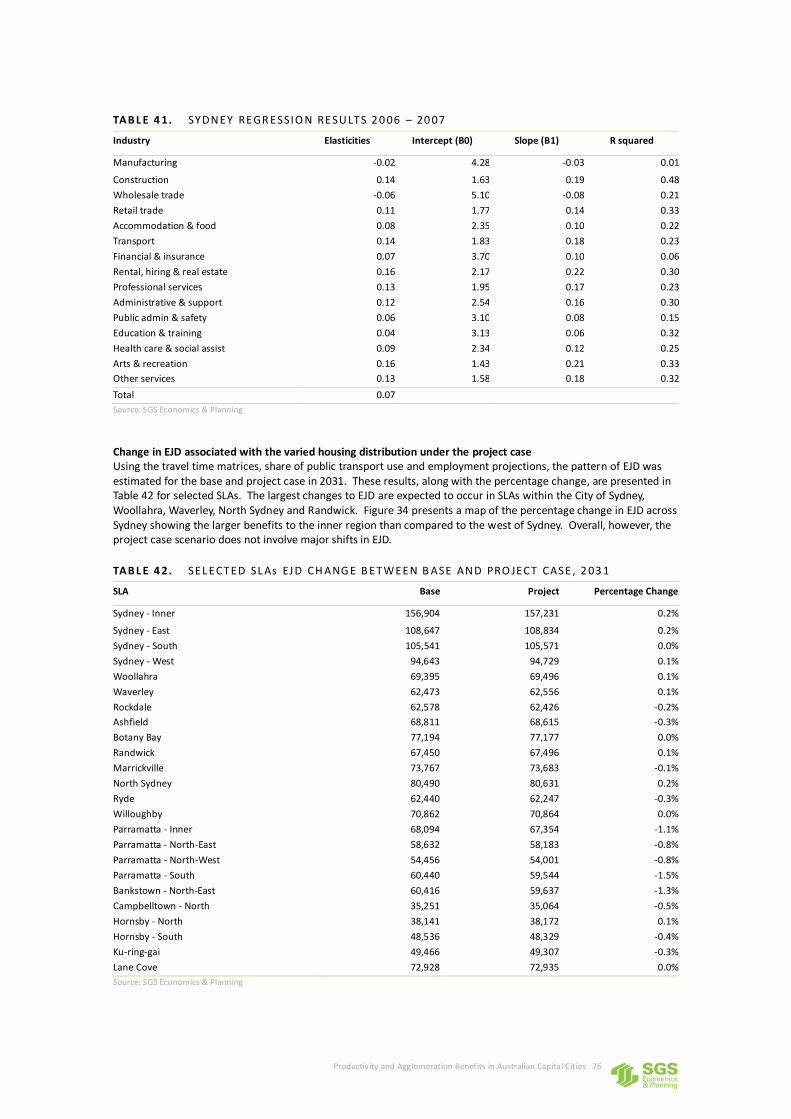
Productivity and Agglomeration Benefits in Australian Capital Cities 76
TAB L E 4 1. SYDNEY REGR ESSIO N RESU LTS 2 0 06 – 20 07
Industry Elasticities Intercept (B0) Slope (B1) R squared
Manufacturing -0.02 4.28 -0.03 0.01
Construction 0.14 1.63 0.19 0.48
Wholesale trade -0.06 5.10 -0.08 0.21
Retail trade 0.11 1.77 0.14 0.33
Accommodation & food 0.08 2.35 0.10 0.22
Transport 0.14 1.83 0.18 0.23
Financial & insurance 0.07 3.70 0.10 0.06
Rental, hiring & real estate 0.16 2.17 0.22 0.30
Professional services 0.13 1.95 0.17 0.23
Administrative & support 0.12 2.54 0.16 0.30
Public admin & safety 0.06 3.10 0.08 0.15
Education & training 0.04 3.13 0.06 0.32
Health care & social assist 0.09 2.34 0.12 0.25
Arts & recreation 0.16 1.43 0.21 0.33
Other services 0.13 1.58 0.18 0.32
Total 0.07
Source: SGS Economics & Planning
Change in EJD associated with the varied housing distribution under the project case Using the travel time matrices, share of public transport use and employment projections, the pattern of EJD was estimated for the base and project case in 2031. These results, along with the percentage change, are presented in Table 42 for selected SLAs. The largest changes to EJD are expected to occur in SLAs within the City of Sydney, Woollahra, Waverley, North Sydney and Randwick. Figure 34 presents a map of the percentage change in EJD across Sydney showing the larger benefits to the inner region than compared to the west of Sydney. Overall, however, the project case scenario does not involve major shifts in EJD.
TAB L E 4 2. SEL ECTED SL As EJ D CH ANG E B ETWEEN B ASE AND PRO JECT CASE , 2 03 1
SLA Base Project Percentage Change
Sydney - Inner 156,904 157,231 0.2%
Sydney - East 108,647 108,834 0.2%
Sydney - South 105,541 105,571 0.0%
Sydney - West 94,643 94,729 0.1%
Woollahra 69,395 69,496 0.1%
Waverley 62,473 62,556 0.1%
Rockdale 62,578 62,426 -0.2%
Ashfield 68,811 68,615 -0.3%
Botany Bay 77,194 77,177 0.0%
Randwick 67,450 67,496 0.1%
Marrickville 73,767 73,683 -0.1%
North Sydney 80,490 80,631 0.2%
Ryde 62,440 62,247 -0.3%
Willoughby 70,862 70,864 0.0%
Parramatta - Inner 68,094 67,354 -1.1%
Parramatta - North-East 58,632 58,183 -0.8%
Parramatta - North-West 54,456 54,001 -0.8%
Parramatta - South 60,440 59,544 -1.5%
Bankstown - North-East 60,416 59,637 -1.3%
Campbelltown - North 35,251 35,064 -0.5%
Hornsby - North 38,141 38,172 0.1%
Hornsby - South 48,536 48,329 -0.4%
Ku-ring-gai 49,466 49,307 -0.3%
Lane Cove 72,928 72,935 0.0%
Source: SGS Economics & Planning
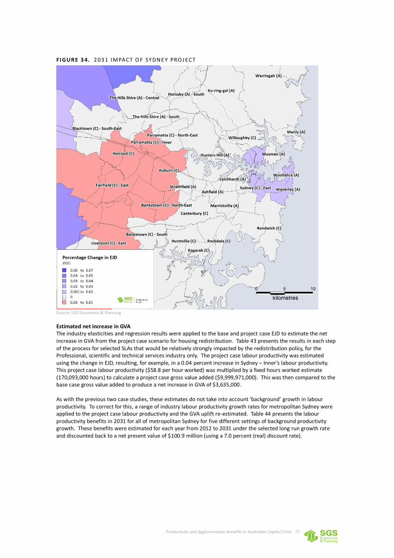
Productivity and Agglomeration Benefits in Australian Capital Cities 77
FI G UR E 3 4. 2 03 1 IMPACT O F SYDNE Y PRO J ECT
Source: SGS Economics & Planning
Estimated net increase in GVA The industry elasticities and regression results were applied to the base and project case EJD to estimate the net increase in GVA from the project case scenario for housing redistribution. Table 43 presents the results in each step of the process for selected SLAs that would be relatively strongly impacted by the redistribution policy, for the Professional, scientific and technical services industry only. The project case labour productivity was estimated using the change in EJD, resulting, for example, in a 0.04 percent increase in Sydney – Inner’s labour productivity. This project case labour productivity ($58.8 per hour worked) was multiplied by a fixed hours worked estimate (170,093,000 hours) to calculate a project case gross value added ($9,999,971,000). This was then compared to the base case gross value added to produce a net increase in GVA of $3,635,000. As with the previous two case studies, these estimates do not take into account ‘background’ growth in labour productivity. To correct for this, a range of industry labour productivity growth rates for metropolitan Sydney were applied to the project case labour productivity and the GVA uplift re-estimated. Table 44 presents the labour productivity benefits in 2031 for all of metropolitan Sydney for five different settings of background productivity growth. These benefits were estimated for each year from 2012 to 2031 under the selected long run growth rate and discounted back to a net present value of $100.9 million (using a 7.0 percent (real) discount rate).
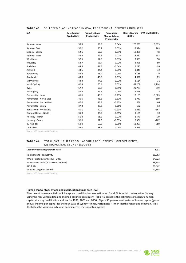
Productivity and Agglomeration Benefits in Australian Capital Cities 78
TAB L E 4 3. SEL ECTED SL AS INCR EA SE IN G VA, PRO FESSIO NAL SER VICES INDU STR Y
SLA Base Labour Productivity
Project Labour Productivity
Percentage
Change Labour Productivity
Hours Worked (000’s)
GVA Uplift (000’s)
Sydney - Inner 58.8 58.8 0.04% 170,093 3,635
Sydney - East 50.2 50.2 0.03% 17,874 269
Sydney - South 52.5 52.5 0.01% 18,385 48
Sydney - West 52.3 52.3 0.02% 18,432 153
Woollahra 57.5 57.5 0.03% 3,963 58
Waverley 53.7 53.7 0.02% 3,998 50
Rockdale 44.5 44.5 -0.04% 5,247 -99
Ashfield 44.5 44.4 -0.05% 1,449 -32
Botany Bay 45.4 45.4 0.00% 3,186 -6
Randwick 49.8 49.8 0.01% 4,950 29
Marrickville 44.3 44.3 -0.02% 3,514 -31
North Sydney 60.4 60.4 0.03% 68,209 1,264
Ryde 57.2 57.2 -0.05% 29,733 -919
Willoughby 57.5 57.5 0.00% 19,818 5
Parramatta - Inner 46.6 46.5 -0.19% 12,185 -1,083
Parramatta - North-East 46.6 46.5 -0.13% 1,741 -109
Parramatta - North-West 47.0 46.9 -0.15% 956 -66
Parramatta - South 37.3 37.2 -0.26% 632 -62
Bankstown - North-East 40.1 40.0 -0.23% 1,833 -167
Campbelltown - North 35.9 35.9 -0.09% 1,165 -39
Hornsby - North 51.8 51.9 0.01% 2,570 19
Hornsby - South 52.0 52.0 -0.07% 5,306 -207
Ku-ring-gai 59.9 59.9 -0.06% 11,261 -380
Lane Cove 58.7 58.7 0.00% 7,613 7
Source: SGS Economics & Planning
TAB L E 4 4. TOTAL G VA UP L IFT FRO M L AB O UR PRO DU CTIV IT Y IMPRO VEMENTS, METR OP OL ITAN SYDNEY ( $0 00 ’S)
Labour Productivity Growth Rate 2031
No Change to Productivity 26,563
Whole Period Growth 1995 - 2010 34,922
Most Recent Cycle (2003-04 to 2009-10) 39,235
IGR 1.5% 38,542
Selected Long Run Growth 40,355
Source: SGS Economics & Planning
Human capital stock by age and qualification (small area level) The current human capital stock by age and qualification was estimated for all SLAs within metropolitan Sydney using the ABS Census data and method outlined previously. Table 45 presents the estimates of Sydney’s human capital stock by qualification and sex for 1996, 2001 and 2006. Figure 35 presents estimates of human capital (gross annual income per capita) for the four SLAs of Sydney – Inner, Parramatta – Inner, North Sydney and Mosman. This illustrates the variation in human capital across metropolitan Sydney.
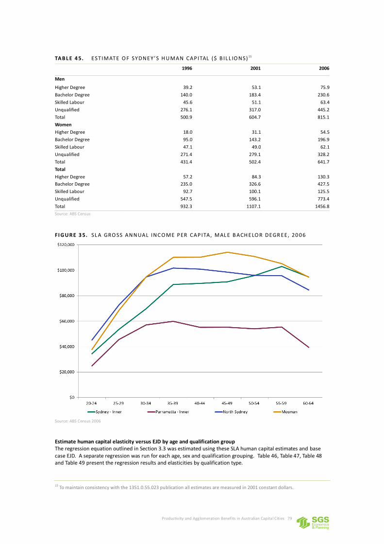
Productivity and Agglomeration Benefits in Australian Capital Cities 79
TAB L E 4 5. EST IMATE O F SYDNEY’S H U MAN CAP ITAL ($ B IL L IO NS) 15
1996 2001 2006
Men
Higher Degree 39.2 53.1 75.9
Bachelor Degree 140.0 183.4 230.6
Skilled Labour 45.6 51.1 63.4
Unqualified 276.1 317.0 445.2
Total 500.9 604.7 815.1
Women
Higher Degree 18.0 31.1 54.5
Bachelor Degree 95.0 143.2 196.9
Skilled Labour 47.1 49.0 62.1
Unqualified 271.4 279.1 328.2
Total 431.4 502.4 641.7
Total
Higher Degree 57.2 84.3 130.3
Bachelor Degree 235.0 326.6 427.5
Skilled Labour 92.7 100.1 125.5
Unqualified 547.5 596.1 773.4
Total 932.3 1107.1 1456.8
Source: ABS Census
F I G UR E 3 5. SL A GRO SS ANNUAL INC O ME P ER CAP ITA, MAL E B ACH ELO R DEGR EE, 20 0 6
Source: ABS Census 2006
Estimate human capital elasticity versus EJD by age and qualification group The regression equation outlined in Section 3.3 was estimated using these SLA human capital estimates and base case EJD. A separate regression was run for each age, sex and qualification grouping. Table 46, Table 47, Table 48 and Table 49 present the regression results and elasticities by qualification type.
15 To maintain consistency with the 1351.0.55.023 publication all estimates are measured in 2001 constant dollars.
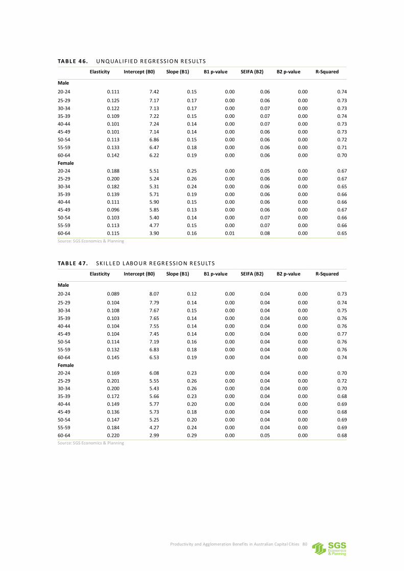
Productivity and Agglomeration Benefits in Australian Capital Cities 80
TA B L E 4 6. U NQ UAL IFIED R EGR ESSI O N R ESU LTS
Elasticity Intercept (B0) Slope (B1) B1 p-value SEIFA (B2) B2 p-value R-Squared
Male
20-24 0.111 7.42 0.15 0.00 0.06 0.00 0.74
25-29 0.125 7.17 0.17 0.00 0.06 0.00 0.73
30-34 0.122 7.13 0.17 0.00 0.07 0.00 0.73
35-39 0.109 7.22 0.15 0.00 0.07 0.00 0.74
40-44 0.101 7.24 0.14 0.00 0.07 0.00 0.73
45-49 0.101 7.14 0.14 0.00 0.06 0.00 0.73
50-54 0.113 6.86 0.15 0.00 0.06 0.00 0.72
55-59 0.133 6.47 0.18 0.00 0.06 0.00 0.71
60-64 0.142 6.22 0.19 0.00 0.06 0.00 0.70
Female
20-24 0.188 5.51 0.25 0.00 0.05 0.00 0.67
25-29 0.200 5.24 0.26 0.00 0.06 0.00 0.67
30-34 0.182 5.31 0.24 0.00 0.06 0.00 0.65
35-39 0.139 5.71 0.19 0.00 0.06 0.00 0.66
40-44 0.111 5.90 0.15 0.00 0.06 0.00 0.66
45-49 0.096 5.85 0.13 0.00 0.06 0.00 0.67
50-54 0.103 5.40 0.14 0.00 0.07 0.00 0.66
55-59 0.113 4.77 0.15 0.00 0.07 0.00 0.66
60-64 0.115 3.90 0.16 0.01 0.08 0.00 0.65
Source: SGS Economics & Planning
TAB L E 4 7. SK IL L ED L ABO U R R EGR E SSIO N R ESU LTS
Elasticity Intercept (B0) Slope (B1) B1 p-value SEIFA (B2) B2 p-value R-Squared
Male
20-24 0.089 8.07 0.12 0.00 0.04 0.00 0.73
25-29 0.104 7.79 0.14 0.00 0.04 0.00 0.74
30-34 0.108 7.67 0.15 0.00 0.04 0.00 0.75
35-39 0.103 7.65 0.14 0.00 0.04 0.00 0.76
40-44 0.104 7.55 0.14 0.00 0.04 0.00 0.76
45-49 0.104 7.45 0.14 0.00 0.04 0.00 0.77
50-54 0.114 7.19 0.16 0.00 0.04 0.00 0.76
55-59 0.132 6.83 0.18 0.00 0.04 0.00 0.76
60-64 0.145 6.53 0.19 0.00 0.04 0.00 0.74
Female
20-24 0.169 6.08 0.23 0.00 0.04 0.00 0.70
25-29 0.201 5.55 0.26 0.00 0.04 0.00 0.72
30-34 0.200 5.43 0.26 0.00 0.04 0.00 0.70
35-39 0.172 5.66 0.23 0.00 0.04 0.00 0.68
40-44 0.149 5.77 0.20 0.00 0.04 0.00 0.69
45-49 0.136 5.73 0.18 0.00 0.04 0.00 0.68
50-54 0.147 5.25 0.20 0.00 0.04 0.00 0.69
55-59 0.184 4.27 0.24 0.00 0.04 0.00 0.69
60-64 0.220 2.99 0.29 0.00 0.05 0.00 0.68
Source: SGS Economics & Planning
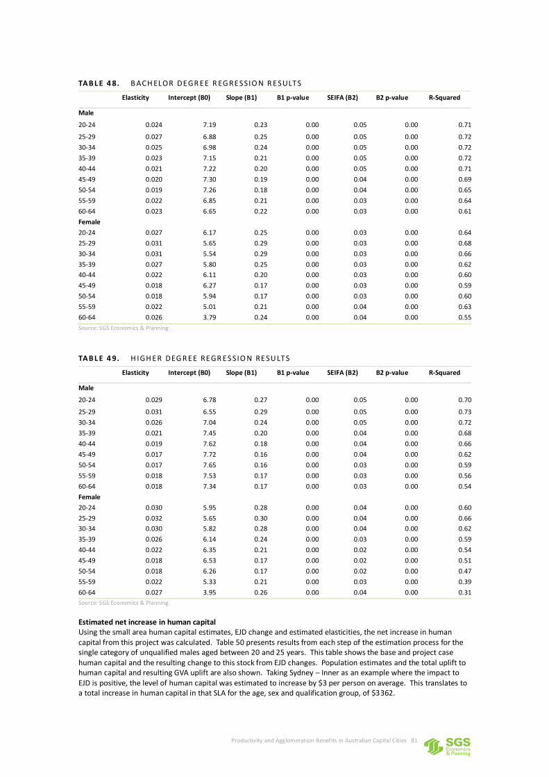
Productivity and Agglomeration Benefits in Australian Capital Cities 81
TAB L E 4 8. B ACH ELOR DEGR EE R EG RESSIO N R ESULTS
Elasticity Intercept (B0) Slope (B1) B1 p-value SEIFA (B2) B2 p-value R-Squared
Male
20-24 0.024 7.19 0.23 0.00 0.05 0.00 0.71
25-29 0.027 6.88 0.25 0.00 0.05 0.00 0.72
30-34 0.025 6.98 0.24 0.00 0.05 0.00 0.72
35-39 0.023 7.15 0.21 0.00 0.05 0.00 0.72
40-44 0.021 7.22 0.20 0.00 0.05 0.00 0.71
45-49 0.020 7.30 0.19 0.00 0.04 0.00 0.69
50-54 0.019 7.26 0.18 0.00 0.04 0.00 0.65
55-59 0.022 6.85 0.21 0.00 0.03 0.00 0.64
60-64 0.023 6.65 0.22 0.00 0.03 0.00 0.61
Female
20-24 0.027 6.17 0.25 0.00 0.03 0.00 0.64
25-29 0.031 5.65 0.29 0.00 0.03 0.00 0.68
30-34 0.031 5.54 0.29 0.00 0.03 0.00 0.66
35-39 0.027 5.80 0.25 0.00 0.03 0.00 0.62
40-44 0.022 6.11 0.20 0.00 0.03 0.00 0.60
45-49 0.018 6.27 0.17 0.00 0.03 0.00 0.59
50-54 0.018 5.94 0.17 0.00 0.03 0.00 0.60
55-59 0.022 5.01 0.21 0.00 0.04 0.00 0.63
60-64 0.026 3.79 0.24 0.00 0.04 0.00 0.55
Source: SGS Economics & Planning
TAB L E 4 9. H IGH ER DEG R EE REGR ES SIO N RESU LTS
Elasticity Intercept (B0) Slope (B1) B1 p-value SEIFA (B2) B2 p-value R-Squared
Male
20-24 0.029 6.78 0.27 0.00 0.05 0.00 0.70
25-29 0.031 6.55 0.29 0.00 0.05 0.00 0.73
30-34 0.026 7.04 0.24 0.00 0.05 0.00 0.72
35-39 0.021 7.45 0.20 0.00 0.04 0.00 0.68
40-44 0.019 7.62 0.18 0.00 0.04 0.00 0.66
45-49 0.017 7.72 0.16 0.00 0.04 0.00 0.62
50-54 0.017 7.65 0.16 0.00 0.03 0.00 0.59
55-59 0.018 7.53 0.17 0.00 0.03 0.00 0.56
60-64 0.018 7.34 0.17 0.00 0.03 0.00 0.54
Female
20-24 0.030 5.95 0.28 0.00 0.04 0.00 0.60
25-29 0.032 5.65 0.30 0.00 0.04 0.00 0.66
30-34 0.030 5.82 0.28 0.00 0.04 0.00 0.62
35-39 0.026 6.14 0.24 0.00 0.03 0.00 0.59
40-44 0.022 6.35 0.21 0.00 0.02 0.00 0.54
45-49 0.018 6.53 0.17 0.00 0.02 0.00 0.51
50-54 0.018 6.26 0.17 0.00 0.02 0.00 0.47
55-59 0.022 5.33 0.21 0.00 0.03 0.00 0.39
60-64 0.027 3.95 0.26 0.00 0.04 0.00 0.31
Source: SGS Economics & Planning
Estimated net increase in human capital Using the small area human capital estimates, EJD change and estimated elasticities, the net increase in human capital from this project was calculated. Table 50 presents results from each step of the estimation process for the single category of unqualified males aged between 20 and 25 years. This table shows the base and project case human capital and the resulting change to this stock from EJD changes. Population estimates and the total uplift to human capital and resulting GVA uplift are also shown. Taking Sydney – Inner as an example where the impact to EJD is positive, the level of human capital was estimated to increase by $3 per person on average. This translates to a total increase in human capital in that SLA for the age, sex and qualification group, of $3362.
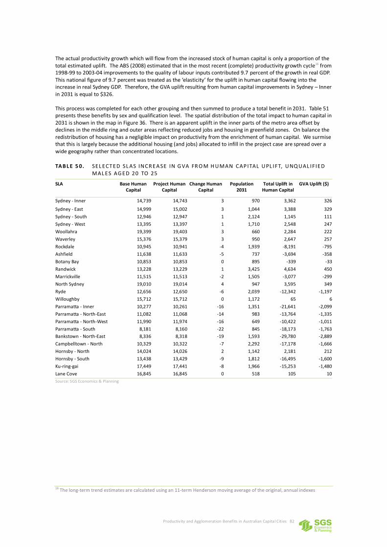
Productivity and Agglomeration Benefits in Australian Capital Cities 82
The actual productivity growth which will flow from the increased stock of human capital is only a proportion of the total estimated uplift. The ABS (2008) estimated that in the most recent (complete) productivity growth cycle16 from 1998-99 to 2003-04 improvements to the quality of labour inputs contributed 9.7 percent of the growth in real GDP. This national figure of 9.7 percent was treated as the ‘elasticity’ for the uplift in human capital flowing into the increase in real Sydney GDP. Therefore, the GVA uplift resulting from human capital improvements in Sydney – Inner in 2031 is equal to $326. This process was completed for each other grouping and then summed to produce a total benefit in 2031. Table 51 presents these benefits by sex and qualification level. The spatial distribution of the total impact to human capital in 2031 is shown in the map in Figure 36. There is an apparent uplift in the inner parts of the metro area offset by declines in the middle ring and outer areas reflecting reduced jobs and housing in greenfield zones. On balance the redistribution of housing has a negligible impact on productivity from the enrichment of human capital. We surmise that this is largely because the additional housing (and jobs) allocated to infill in the project case are spread over a wide geography rather than concentrated locations.
TAB L E 5 0. SEL ECTED SL AS INCR EA SE IN G VA FR O M H U MAN CAP ITAL U PL IFT, U NQ UAL IFIED MAL ES AG ED 20 TO 25
SLA Base Human Capital
Project Human Capital
Change Human Capital
Population 2031
Total Uplift in Human Capital
GVA Uplift ($)
Sydney - Inner 14,739 14,743 3 970 3,362 326
Sydney - East 14,999 15,002 3 1,044 3,388 329
Sydney - South 12,946 12,947 1 2,124 1,145 111
Sydney - West 13,395 13,397 1 1,710 2,548 247
Woollahra 19,399 19,403 3 660 2,284 222
Waverley 15,376 15,379 3 950 2,647 257
Rockdale 10,945 10,941 -4 1,939 -8,191 -795
Ashfield 11,638 11,633 -5 737 -3,694 -358
Botany Bay 10,853 10,853 0 895 -339 -33
Randwick 13,228 13,229 1 3,425 4,634 450
Marrickville 11,515 11,513 -2 1,505 -3,077 -299
North Sydney 19,010 19,014 4 947 3,595 349
Ryde 12,656 12,650 -6 2,039 -12,342 -1,197
Willoughby 15,712 15,712 0 1,172 65 6
Parramatta - Inner 10,277 10,261 -16 1,351 -21,641 -2,099
Parramatta - North-East 11,082 11,068 -14 983 -13,764 -1,335
Parramatta - North-West 11,990 11,974 -16 649 -10,422 -1,011
Parramatta - South 8,181 8,160 -22 845 -18,173 -1,763
Bankstown - North-East 8,336 8,318 -19 1,593 -29,780 -2,889
Campbelltown - North 10,329 10,322 -7 2,292 -17,178 -1,666
Hornsby - North 14,024 14,026 2 1,142 2,181 212
Hornsby - South 13,438 13,429 -9 1,812 -16,495 -1,600
Ku-ring-gai 17,449 17,441 -8 1,966 -15,253 -1,480
Lane Cove 16,845 16,845 0 518 105 10
Source: SGS Economics & Planning
16 The long-term trend estimates are calculated using an 11-term Henderson moving average of the original, annual indexes
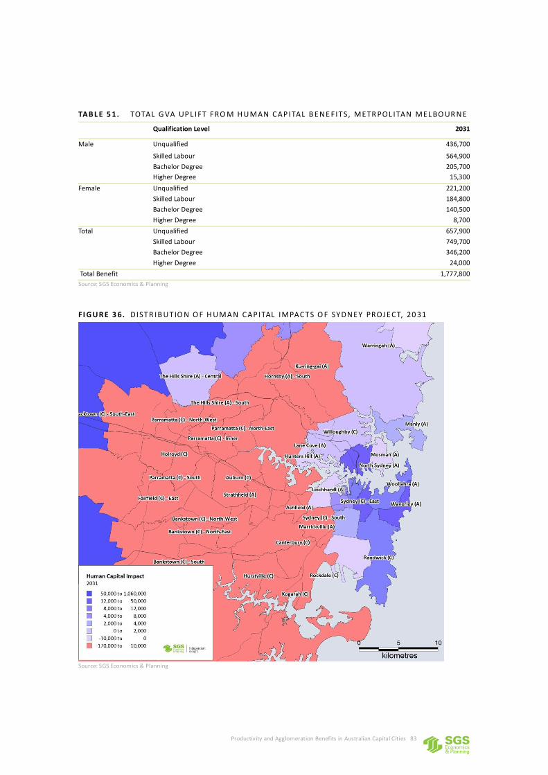
Productivity and Agglomeration Benefits in Australian Capital Cities 83
TAB L E 5 1. TOTAL G VA UP L IFT FRO M H U MAN CAP ITAL B ENE FITS, METR POL ITAN MEL BO UR NE
Qualification Level 2031
Male Unqualified 436,700
Skilled Labour 564,900
Bachelor Degree 205,700
Higher Degree 15,300
Female Unqualified 221,200
Skilled Labour 184,800
Bachelor Degree 140,500
Higher Degree 8,700
Total Unqualified 657,900
Skilled Labour 749,700
Bachelor Degree 346,200
Higher Degree 24,000
Total Benefit 1,777,800
Source: SGS Economics & Planning
FI G UR E 3 6. DISTR IB U TIO N O F H U MA N CAP ITAL IMPACTS O F SYDNEY PROJ ECT, 20 31
Source: SGS Economics & Planning

Productivity and Agglomeration Benefits in Australian Capital Cities 84
4 A RESEARCH AGENDA FOR AUSTRALIA
For the most part, theory and evidence on agglomeration provide convincing arguments which support a significant relationship between economic density and productivity. Nevertheless, there are a number of gaps within the research body and conceptual measurement issues are evident. The links between agglomeration, macroeconomic theory and GDP are not as well researched as the micro-economic foundations of the urban agglomeration idea. A key gap is the theoretical and empirical understanding of how agglomeration contributes to per capita consumption. Rossi-Hansberg and Wright’s (2007) work demonstrates how localisation economies can affect aggregate total factor productivity (p. 616). However, more work is required to better understand the empirical relationship between government policy, urban structure and productivity. The conceptual framework and methods set out in this report and illustrated in the case studies provide something of a starting point for developing this improved understanding in an Australian context. In advancing this understanding, a number of data gaps and methodological dilemmas need to be addressed. These are discussed in this section.
4.1 Research issues - productivity effects of agglomeration
Effective density correlated with other explanatory factors
The methodology explained and demonstrated in this report delivers findings broadly in line with the international literature with respect to the elasticity of productivity versus an index of effective density. This is reassuring. However, the same international literature points to the possibility that the explanatory variable of effective density may be a proxy for, or move with, other factors which influence the geography of higher productivity firms. For example, there may be a ‘selection’ process in place whereby only more productive firms survive in the more intense competitive environment of dense urban centres. Similarly, higher productivity firms may ‘sort’ themselves into central, higher rent, locations simply because they have superior capacity to pay for these scarcer locations. These hypothesised processes raise the question of the direction of causality in the effective density / productivity equation. That is to say, rather than firms being more productive because they are in a central location, firms that are more productive can command central locations. Sorting and selection may obscure the true effect of agglomeration on productivity. Moreover, it is difficult to disentangle these various influences on the spatial patterning of productivity. Firms which are outcompeting less productive agents for high EJD locations are, presumably, gaining off-setting benefits for the additional costs incurred. This, in itself, points to the prospect of external benefits for these top-bidder firms in the form of superior access to skills or suppliers – the very stuff of agglomeration economies. Some recent studies, most notably Mare and Graham (2009), have sought to isolate the impact of agglomeration versus sorting and selection by examining productivity and effective density patterns for enterprises that are closely matched in all aspects other than location. These tend to show a dampening of the agglomeration elasticities though they remain in evidence. Similar studies are warranted in Australia, but will require micro-level data which is not currently available to researchers.
Use of cross sectional data to assess future productivity impacts
As discussed in the case studies (Section 3), productivity versus agglomeration elasticities are generated from cross-sectional data, that is, by examining variations in productivity within a given sector with respect to effective density at a particular point in time. This elasticity is then applied to a prospective change in the pattern of effective density to simulate the net productivity impact associated with a transport intervention or land use strategy.

Productivity and Agglomeration Benefits in Australian Capital Cities 85
The fact that reported elasticities for Australian cities (7 percent to 9 percent for the case studies discussed here) are in the midpoint of the international literature is, again, reassuring and may point to some form of stable linear relationship. This, in turn, provides some comfort that applying a fixed productivity elasticity to future changes in effective density is defensible. However, empirical investigation of this hypothesis is called for. Retrospective studies of the impacts of past major transport investments could shed some light on these issues. We note from the literature that there is limited understanding on the question of whether there is a ‘cap’ to agglomeration, and at what point, if any, the returns to economic densification may become evident. For example, in a bustling metropolis, centrifugal forces as defined by Krugman (1998) may lead to diminishing returns and discourage further agglomeration.
Data on productivity at the firm level
The principal opportunity for strengthening the methodology set out in this report is the assembly of better data on firm productivity at the small area level. At present this information must be inferred from national and state level productivity data. The estimation of productivity variations in the presence of capital intensity is particularly challenging (see further discussion below). The landmark studies conducted in the UK (Graham, 2006) and New Zealand (Mare and Graham, 2009) have had the benefit of detailed micro level data on firm activity and performance. According to the Department of Transport Victoria (2012), similar data sets exist in Australia but have not yet been made available to researchers. The Department points to the possibility of tracking the behaviour of nine thousand firms in Australia over the six years 2004-05 to 2009-10 through the ABS Business Longitudinal Database. Public access to this database is currently highly restricted. It includes business addresses which may be geocoded to enable detailed spatial analysis. The Department further reports that the ABS business database has direct access to Australian Taxation Office (ATO) quarterly Business Activity Statement returns for profitability and also links with Customs and Excise information. There may be other sources for firm level productivity data accessible at the state and territory jurisdictional level, for example, databases held by payroll tax and worker insurance authorities. Unlocking access to this micro-level data, with suitable confidentiality safeguards, would represent a break-through for agglomeration and productivity research in Australia. It should be a priority for jurisdictions.
Refining the measures of effective density and productivity
The index of agglomeration used in the case studies – effective job density – is currently all embracing; it bundles all jobs regardless of their anticipated relevance to a particular sector. In this context, measuring the benefits of agglomeration and human capital improvements for that matter can face two challenges, depending on whether a single industry or multiple industries are analysed. Within a single industry, there can be significant variations in gross value added (that is, productivity) per worker reflecting micro-classification considerations. For example, within the ‘finance industry’, the occupations of bank teller and investment banker would demonstrate different levels of gross value added. The second challenge is when measuring across industries. Some industries are more capital and technology intensive, and this reliance on capital and technology can be reflected in apparent human capital improvements. For example, a telecommunications technician may be more productive following upgrades to key software and hardware. In contrast, occupations within the law, for example, may be far less reliant on capital and technology. In this sense, it can be difficult to distinguish between the contributions of human capital enrichment and technological advancements to improved productivity per worker. One approach to addressing this issue is to attribute weightings to different industries or occupations. A weighting system could also be used to separate out population-driven occupations from the effective density index. Industries such as personal services and retail tend to follow population movements. Including these industries in an estimation of productivity gains from agglomeration may not be entirely appropriate. These strategies to account for capital intensity and to focus on relevant agglomerations of business require testing, preferably with the micro-data sets noted above.

Productivity and Agglomeration Benefits in Australian Capital Cities 86
4.2 Research issues – human capital
Double counting with productivity effects
As noted in Section 1.1, consideration of the human capital boosting effect of major infrastructure projects lies at the frontier of agglomeration research and is an area where Australian research is, arguably, breaking new ground. The hypothesis is that if households can be characterised as ‘knowledge intensive’ enterprises in their own right – an increasingly uncontroversial proposition in Australia’s substantially de-regulated labour market – they should benefit from the same productivity boosting effects of greater economic connectivity and density. This report demonstrates one technique for measuring this uplift in household productivity, or increase in human capital. Thus far, this hypothesis has not been refuted in the literature on theoretical or conceptual grounds. However, the question of double counting with the estimated increase in labour productivity at the firm level looms large. On the face of things, some degree of double counting appears likely. If the business locations of relatively high productivity firms and residential locations of their workers are broadly aligned, the human capital boost enjoyed by households from agglomeration (that is, the margin in wages and salaries) will also be recorded in the higher gross operating surpluses of firms in high EJD areas. This question of additivity of human capital impacts requires further research. Resolving the degree of any double counting is only part of the research challenge. It ought not be overlooked that some of the increase in human capital occasioned by urban agglomeration will not be reflected in labour productivity at the firm level simply because many able people are not in the workforce, often by choice. The fact that these people enjoy agglomeration boosted skills but are not working does not mean that the increase in human capital does not add to welfare. The people in question may be better, more engaged, citizens leading to better communities and more effective governance. Moreover, some of these boosted skills are transportable and transferable. In this sense, separate measurement of the human capital effects of agglomeration are warranted, even if they are reported alongside, rather than in addition to, labour productivity at the firm level.
Direction of causality
The same selection and sorting issues which confound interpretation of the links between effective density and labour productivity are present with respect to the human capital effects of agglomeration. Higher income households may simply be outbidding other households for the more central locations that carry an EJD premium as opposed to the higher EJD ratings driving, in some way, higher incomes other things equal. Again, however, the question arises as to why households would pay more for high EJD locations if these places did not deliver benefits in terms of expanded choices and accelerated skills acquisition. In this regard, it is interesting to note that in at least one major Australian city, Melbourne, high EJD suburbs did not always attract a premium. During those periods of ‘Fordist’ manufacturing expansion, preferred residential locations were often in outer suburban environments offering new housing and/or superior access to natural assets like beaches, hills, views and so on. The house price gradient versus distance from city centre has risen sharply in Melbourne over the past 10 years or so, possibly reflecting the shift to a metropolitan economy powered by technical, scientific and professional services rather than manufacturing (Figure 37). With this shift, expanded opportunities for skills acquisition become ever more important. This may explain enhanced competition for high agglomeration locations compared to previous eras, and the (apparently) strengthening nexus between house prices and EJD (Figure 38). Further research is required to establish whether households are, to some extent, sacrificing suburban amenity to avail themselves of the tacit learning opportunities offered by high EJD locations.
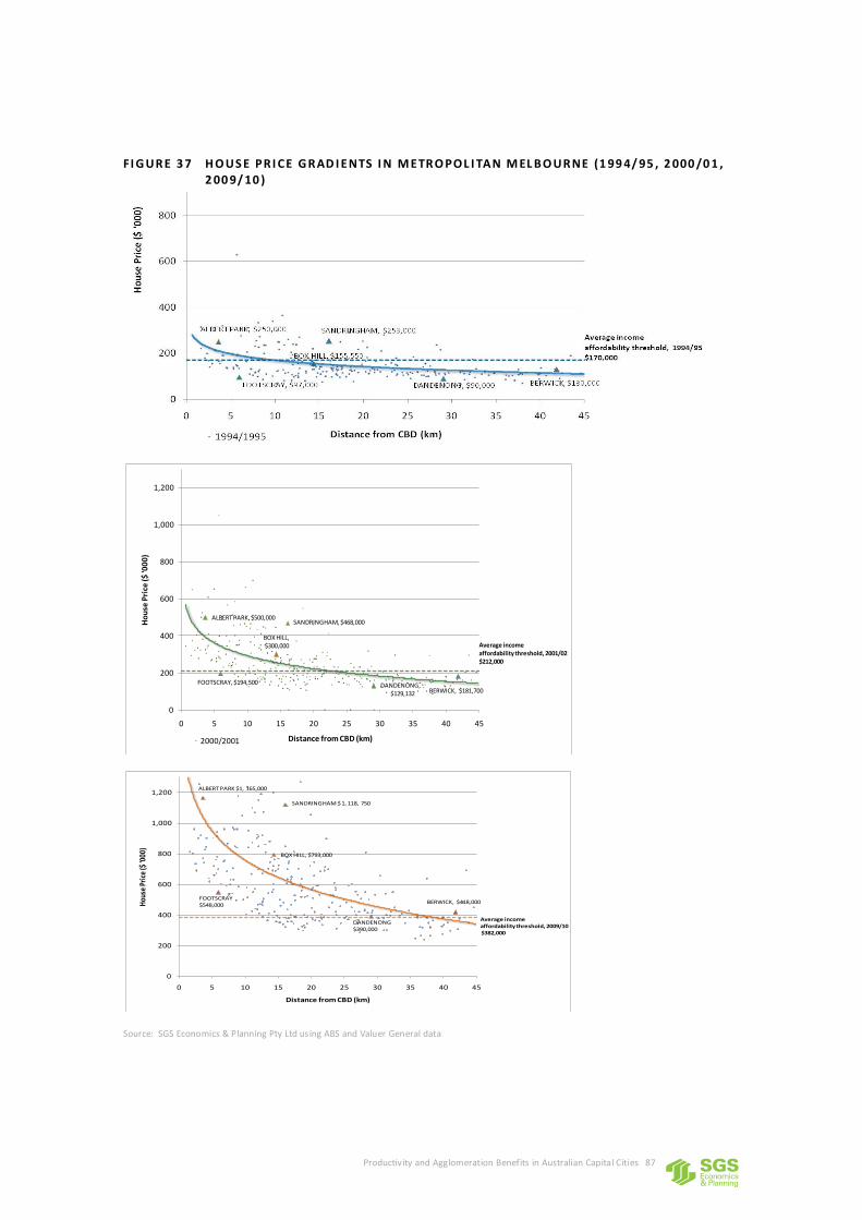
Productivity and Agglomeration Benefits in Australian Capital Cities 87
FI G UR E 3 7 H O US E PR I CE G R AD I ENTS I N M ETR O POL I TAN M EL B O UR NE (1 99 4/ 95 , 2 000 /0 1 , 2 00 9/ 10 )
Source: SGS Economics & Planning Pty Ltd using ABS and Valuer General data
ALBERT PARK, $500,000
BOX HILL,$300,000
0
200
400
600
800
1,000
1,200
0 5 10 15 20 25 30 35 40 45
Ho
use
Pri
ce ($
'00
0)
Distance from CBD (km)2000/2001
Average incomeaffordability threshold, 2001/02$212,000
DANDENONG,$129,132
FOOTSCRAY, $194,500BERWICK, $181,700
SANDRINGHAM, $468,000
BERWICK, $418,000
BOX HILL, $793,000
0
200
400
600
800
1,000
1,200
0 5 10 15 20 25 30 35 40 45
Hou
se P
rice
($ '0
00)
Distance from CBD (km)
Average incomeaffordability threshold, 2009/10$382,000
DANDENONG$390,000
FOOTSCRAY $548,000
SANDRINGHAM $ 1, 118, 750
ALBERT PARK $1, 165,000
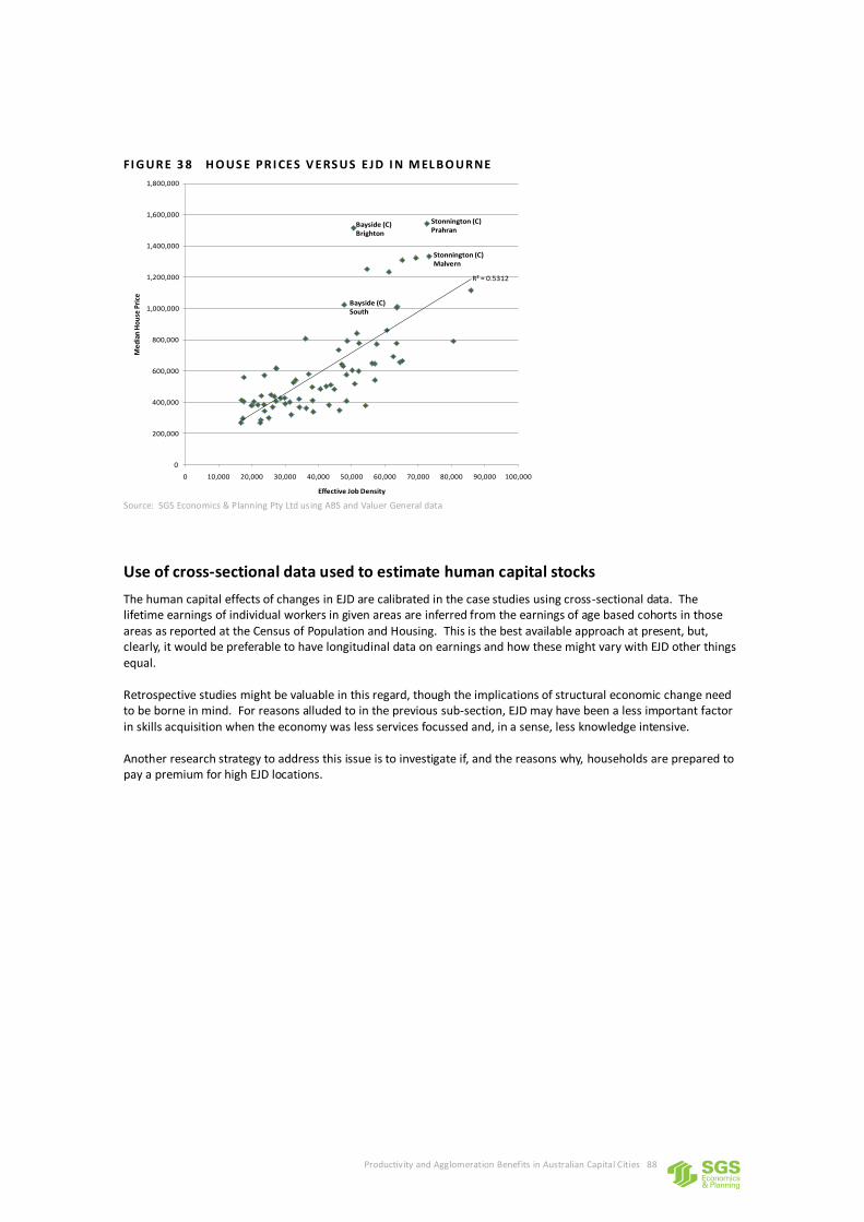
Productivity and Agglomeration Benefits in Australian Capital Cities 88
FI G UR E 3 8 H O US E PR I CES V ERS US EJD I N M EL B O UR NE
Source: SGS Economics & Planning Pty Ltd using ABS and Valuer General data
Use of cross-sectional data used to estimate human capital stocks
The human capital effects of changes in EJD are calibrated in the case studies using cross-sectional data. The lifetime earnings of individual workers in given areas are inferred from the earnings of age based cohorts in those areas as reported at the Census of Population and Housing. This is the best available approach at present, but, clearly, it would be preferable to have longitudinal data on earnings and how these might vary with EJD other things equal. Retrospective studies might be valuable in this regard, though the implications of structural economic change need to be borne in mind. For reasons alluded to in the previous sub-section, EJD may have been a less important factor in skills acquisition when the economy was less services focussed and, in a sense, less knowledge intensive. Another research strategy to address this issue is to investigate if, and the reasons why, households are prepared to pay a premium for high EJD locations.
R² = 0.5312
0
200,000
400,000
600,000
800,000
1,000,000
1,200,000
1,400,000
1,600,000
1,800,000
0 10,000 20,000 30,000 40,000 50,000 60,000 70,000 80,000 90,000 100,000
Me
dia
n H
ou
se P
rice
Effective Job Density
Average - Median House Price vs Effective Job Density (SLA)
Average - Median House Price
Linear (Average - Median House Price)
Bayside (C) South
Bayside (C) Brighton
Stonnington (C)Prahran
Stonnington (C)Malvern
Productivity and Agglomeration Benefits in Australian Capital Cities 89
REFERENCES
Aaberg, Y. (1973): “Regional productivity differences in Swedish manufacturing”, Regional and Urban Economics, 3, 131–56. Aghion, P. and Howitt, P., (1998), Endogenous Growth Theory. Cambridge, MA. MIT Press. Arrow, K.J. (1962) “Economic welfare and the allocation of resources for invention “ in R.R. Nelson, ed., The Rate and Direction of Inventive Activity, Princeton University Press, Princeton 609-626. Audretsch, D.B. and Feldman, M.P. (1996) “R&D spillovers and the geography of innovation and production” American Economic Review 86:3, 630-640. Baumgartner, J.R. (1988) “Physicians’ services and the division of labor across local markets” Journal of Political Economy 96(5): 948-982. Buchanan, P. (2007) The Economic Benefits of CrossRail: Final Report. Colin Buchanan and Volterra, London. Carlot, S. and Duranton, G. (2002) “Communication Externalities in Cities” London School of Economics Working Paper. Chinitz, B.J. (1961) “Contrasts in Agglomeration: New York and Pittsburgh” American Economic Review 51: 279-289. Ciccone, A. and Hall, R.E. (1996) “Productivity and the Density of Economic Activity” American Economic Review 86:54-70. Ciccone, A (2002) “Agglomeration effects in Europe”, European Economic Review 46:213-227. Combes (2000) “Economic Structure and local growth: France, 1984-1993”, Journal of Urban Economics 47: 329-355. Costa, D.L. and Kahn, M.E. (2001) “Power Couples” Quarterly Journal of Economics 116: 1287-1315. Davis, D.R. & Weinstein, D.E.(1996.)"Does Economic Geography Matter for International Specialization?," Harvard Institute of Economic Research Working Papers 1773, Harvard - Institute of Economic Research.. Davis, M.A., Fisher, J.D.M, and Whited, T.M. (2011) “Macroeconomic Implications of Agglomeration”. Discussion paper for the Federal Reserve Bank of Chicago. Dekle, R. And Eaton, J. (1999) “Agglomeration and land rents: evidence from the prefectures” Journal of Urban Economics 46:200-214. Department of Transport (Victoria) (2012) Urban density, productivity and the role of transport; an overview of agglomeration benefits in transport investment appraisal and implications for the transport portfolio. Unpublished working paper Duranton, G. and Overmans, H.G. (2002) “Testing for localisation using micro-geographic data” London School of Economics Working Paper. Eberts, R.W. and P.P. McMillan (1999) “Agglomeration economies and urban public infrastructure” in P. Cheshire and E.S. Mills eds, Handbook of Urban and Regional Economics, Volume 3, North Holland, New York 1455 – 1495. Ellison, G. and Glaeser, E. (1997) “Geographic Concentration in U.S. Manufacturing Industries: A Dartboard Approach” Journal of Political Economy 105: 889-927. Ellison, G. and E. Glaeser (1999) “The geographic concentration of an industry: Does natural advantage explain agglomeration” American Economic Association Papers and Proceedings 89, 311-316.

Productivity and Agglomeration Benefits in Australian Capital Cities 90
European Conference of Transport Ministers, Economic Research Centre (ECMT) 2001. Round Table 119: Transport and Economic Development, France. Glaeser, E.L, Kallal, H.D, Scheinhman, J.A. and Schleifer, A. (1992) “Growth in Cities” Journal of Political Economy 100: 1126-1152. Glaeser, E.L. and Mare, D.C. (2001) “Cities and Skills” Journal of Labor Economics 19(2): 316-342. Graham, D.J. (2006), Wider Economic Benefits of Transport Improvement: Link Between Agglomeration and Productivity, Stage 2 Report, prepared for the Department for Transport, London. Glaeser, E.L. and Resseger, M.G. (2010) “The complementarity between cities and skills” Journal of Regional Science, 50:221-244 Hansen, E.R. (1990) “Agglomeration economies and industrial centralization: The wage – productivity trade offs” Journal of Urban Economics 48:140-159 Hanson, G.H. (1998).”‘Market potential, increasing returns, and geographic concentration.” Working Paper No. 6429, National Bureau of Economic Research. Helsley, R.W. and Strange, W.C. (1990) “Agglomeration Economies and Matching in a System of Cities” Regional Science and Urban Economics 51(1): 25-45. Helsley, R.W. and Strange, W.C. (2001) “Innovation and Input Sharing” Journal of Urban Economics 51(1): 25-45. Henderson, J.V. (1986) “Efficiency of Resource Usage and City Size” Journal of Urban Economics 35: 83 -104. Henderson, J.V, Kurncoro, A. and Turner, M. (1995) “Industrial Development in Cities” Journal of Political Economy 103: 1067-1085. Henderson, J.V. (2003a) “Marshall’s Scale Economics” Journal of Urban Economics 53: 1-28 Henderson, J. V. (2003b) “The Urbanization Process and Economic Growth: The So-What Question” Journal of Economic Growth 8: 47-71. Henry, K. (2010) To Build, Or Not To Build: Infrastructure Challenges in the Years Ahead and the Role of Governments; Address to the Conference on the Economics of Infrastructure in a Globalised World: Issues, Lessons and Future Challenges, 18 March Hensley, R.W. and Strange, W.C. (2002) “Knowledge Barter” University of Toronto Faculty of Management Working Paper. Holmes, T.J. (1999) “Localization of Industry and Vertical Disintegration” Review of Economics and Statistics, 81(2): 314-325. Henderson, Vernon & Kuncoro, Ari & Turner, Matt, 1995. "Industrial Development in Cities," Journal of Political Economy, University of Chicago Press, vol. 103(5), pages 1067-90, October. Henderson, Lee and Lee (2001) “Scale externalities in Korea” Journal of Urban Economics 49:479-504. Infrastructure Australia (2010) Getting the Fundamentals Right for Australia’s Infrastructure Priorities Jacobs, J. (1969) The Economy of Cities, Vintage, New York. Jaffe, A.B, Trajtenberg, M. and Henderson, R. (1993) “Geographic Localization of Knowledge Spillovers as Evidenced by Patent Citations” Quarterly Journal of Economics 108: 577-598 Kim, S. (1995), “Expansion of Markets and the Geographic Distribution of Economic Activities: The Trends in U.S. Regional Manufacturing Structure, 1860-1987” Quarterly Journal of Economics 110(4): 881-908.
Productivity and Agglomeration Benefits in Australian Capital Cities 91
Kim, S. (1999) “Regions, resources and economics geography: Sources of U.S. regional comparative advantage, 1880-1987” Regional Science and Urban Economics, 29: 1-32. Krugman, P.R. (1980) “Scale economies, product differentiation and the pattern of trade” American Economic Review 70:950-9 Krugman, P.R. (1998) “What’s new about the new economic geography?” Oxford Review of Economic Policy, 14:7-17 Mare, D. C. and Graham, D. J. (2009) “Agglomeration Elasticities in New Zealand”, Motu Working Paper 09-06, Motu Economic and Public Policy Research Marshall, A. (1920) Principles of Economics, Macmillan, London. Mincer, J. (1995). Economic Development, Growth of Human Capital, and the Dynamics of the Wage Structure, Journal of Economic Growth, March, pp. 29–48. Moomaw, R.L. (1981) “Productivity and city size: a critique of the evidence” Quarterly Journal of Economics 96: 675 – 688. Moomaw, R. L. (1983) “Is population scale a worthless surrogate for business agglomeration economies?” Regional Science and Urban Economics 13: 525-545. National Cooperative Highway Research Program “Economic Implications of Congestion” NCHRP Report 463, National Academy Press, Washington, D. C. 2001. Nakamura, R. (1985) “Agglomeration economies in urban manufacturing industries: a case of Japanese cities” Journal of Urban Economics 17:108-124. Porter, M. (1990) The Competitive Advantage of Nations, The Free Press, New York. Quigley, J.M. 1998. “Urban Diversity and Economic Growth.” Journal of Economic Perspectives 12: 127-138. Rauch, J. (1993a) “Productivity gains from geographic concentration of human capital: evidence from the cities” Journal of Urban Economics 34: 380-400. Romer, P. (1986) “Increasing Returns and Long Run Growth” Journal of Political Economy 94: 1002-1037. Romer, P.M (1990) “Endogenous Technological Change” Journal of Political Economy, 98:S174-S102 Rosenthal, S.S. and Strange, W.C. (2002) “Geography, Industrial Organization, and Agglomeration” Review of Economics and Statistics 85(2): 377-393. Rossi-Hansberg and Wright (2007) "Establishment Size Dynamics in the Aggregate Economy," American Economic Review, American Economic Association, vol. 97(5), pages 1639-1666, December. Saxenian, A. (1994), Regional Advantage: Culture and Competition in Silicon Valley and Route 128, Harvard University, Cambridge, MA. Shefer, D. (1973) “Localization economies in SMSAs: A production function analysis” Journal of Regional Science 13: 55-64. Simon, C.J. (1988) “Frictional Unemployment and the role of industrial diversity” Quarterly Journal of Economics 103: 715-728. Solow, R.M. (1956) “A contribution to the theory of economic growth” The Quarterly Journal of Economics 70:65-94 Sveikauskas, L. (1975) “The productivity of cities” Quarterly Journal of Economics 89: 393-413. Sveikauskas, L.A, Townroe, P.P., and Hansen, E.R. (1985) “Intraregional Productivity difference in Sao Paulo State Manufacturing Plants” Weltwirtschaftliches Archiv 121:722-40 Swan, T.W. (1956) “Economic Growth and Capital Accumulation” Economic Record 32:335-61

Productivity and Agglomeration Benefits in Australian Capital Cities 92
Tabuchi, T. (1986): ‘Urban agglomeration, capital augmenting technology, and labour market equilibrium’, Journal of Urban Economics, 20, 211–28. Tabuchi, T and Yoshida A. (2000) “Separating Urban Agglomeration Economies in Consumption and Production” Journal of Urban Economics, 48:70-84 Varga, A. (2000) “Local academic knowledge spillovers and the concentration of economic activity”. Journal of Regional Science 40:289-309 Varga, A. (2001) “Universities and regional economic development: Does agglomeration matter? In Johansson, B., Karlsson, C. and Stough, R. (eds) Theories of Endogenous Regional Growth – Lessons for Regional Policies, Springer, Berlin, 345-367 Varga, A. and Schalk, H.J. (2004) “Knowledge spillovers, agglomeration and macroeconomic growth: An empirical approach” Regional Studies 38:977-989 Waldfogel, J. (2003): Preference Externalities: An Empirical Study Of Who Benefits Whom In Differentiated-Product Markets," Rand Journal of Economics, 34(3), 557{568. World Bank (2009) “Reshaping Economic Geography”, World Development Report 2009

Productivity and Agglomeration Benefits in Australian Capital Cities 93

www.sgsep.com.au
Contact us BRISBANE
PO Box 117 Level 1, 76 McLachlan Street Fortitude Valley QLD 4006
+61 7 3124 9026 [email protected]
CANBERRA
Level 1, 55 Woolley Street Dickson ACT 2602
+61 2 6262 7603 [email protected]
HOBART
Unit 2, 5 King Street Bellerive TAS 7018
+61 (0)439 941 934 [email protected]
MELBOURNE
Level 5, 171 La Trobe Street Melbourne VIC 3000
+61 3 8616 0331 [email protected]
SYDNEY
Suite 12, 50 Reservoir Street Surry Hills NSW 2010
+61 2 8307 0121 [email protected]