Problem 1

The corrections can be larger than the anomaly

Stat. TimeT

Dist. (m)

Elev. (m)

Reading(dial units)

Base readingat time T

Drift corr’d anom. (gu)

LC(gu)

FAC(gu)

BC(gu)

Free airanom(gu)

Boug.anom.(gu)

BS 0805 0 0 2934.2 0 0 0

1 0835 20 10.37 2931.3 2934.49 -12.10 -0.16 32.00 -11.73 19.74 8.01

2 0844 40 12.62 2930.6 2934.57 -15.05 -0.32 38.95 -14.28 23.58 9.3

3 0855 60 15.32 2930.4 2934.68 -16.23 -0.48 47.28 -17.34 30.57 13.23

4 0903 80 19.40 2927.2 2934.76 -28.67 -0.63 59.87 -21.95 30.57 8.62

BS 0918 0 0 2934.9 0

Note that the most significant part of the free-air anomaly appear to due to the attraction of the extra material beneath the survey stations, and that when the Bouguer correction is applied the remaining anomaly is quite small and positive – i.e. the rocks below these stations are slightly denser than those below the base station.

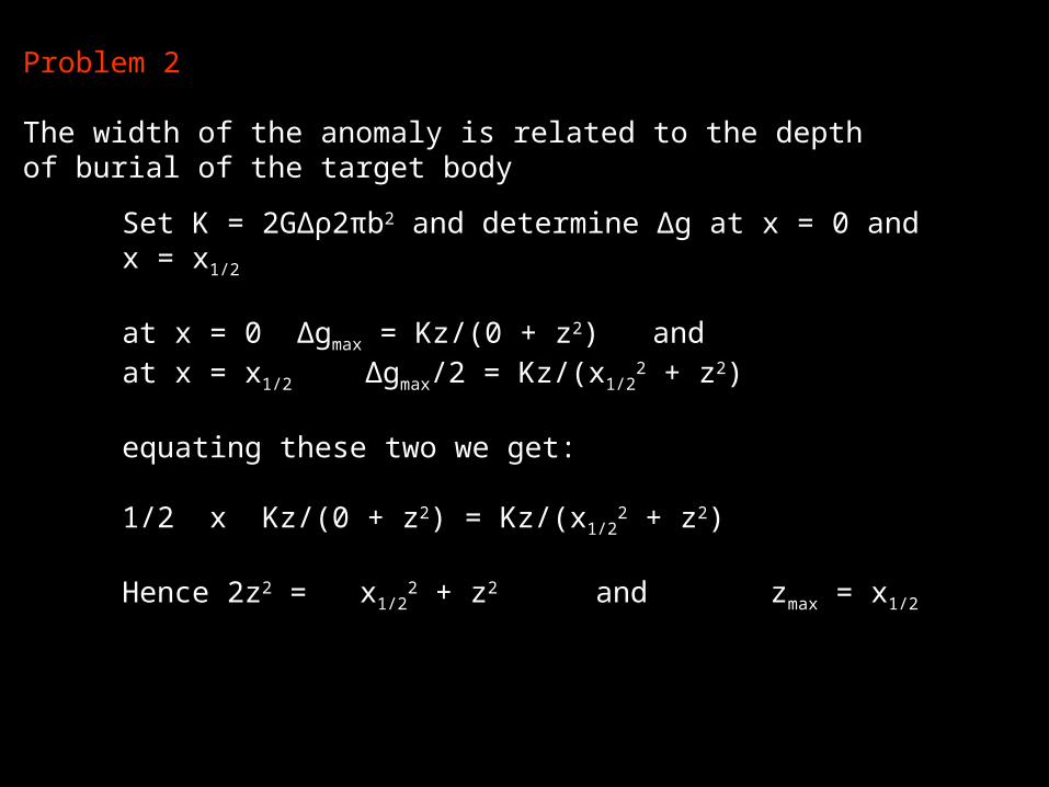
Problem 2

The width of the anomaly is related to the depth of burial of the target body

Set K = 2GΔρ2πb2 and determine Δg at x = 0 and x = x1/2

at x = 0 Δgmax = Kz/(0 + z2) and at x = x1/2 Δgmax/2 = Kz/(x1/2

2 + z2)

equating these two we get:

1/2 x Kz/(0 + z2) = Kz/(x1/22 + z2)

Hence 2z2 = x1/22 + z2 and zmax = x1/2

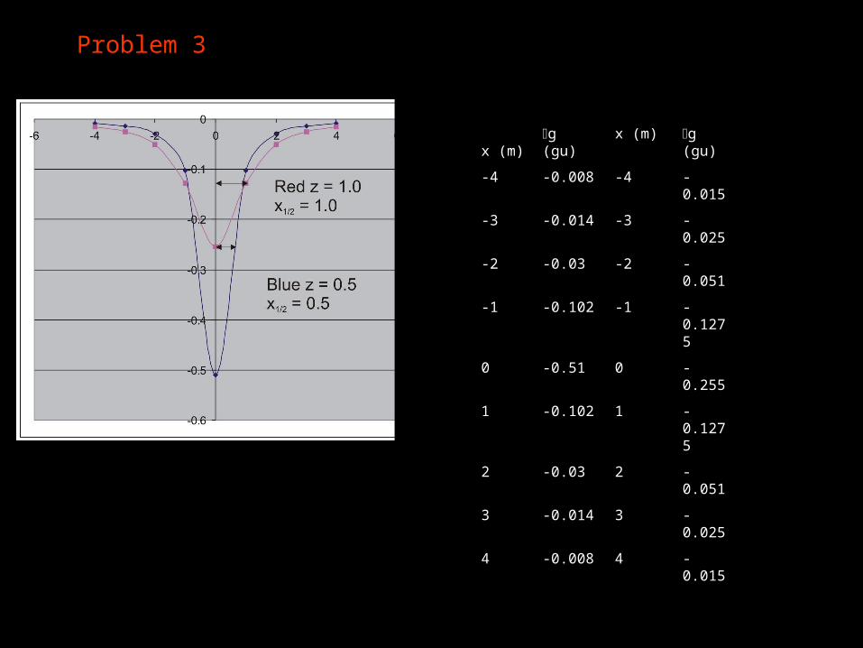
Problem 3

x (m)g (gu) x (m) g (gu)

-4 -0.008 -4 -0.015

-3 -0.014 -3 -0.025

-2 -0.03 -2 -0.051

-1 -0.102 -1 -0.1275

0 -0.51 0 -0.255

1 -0.102 1 -0.1275

2 -0.03 2 -0.051

3 -0.014 3 -0.025

4 -0.008 4 -0.015

Why is it Zmax?If the body were deeper, the width of the anomaly would increase. But you could obtain the same gravity anomaly with other bodies placed at shallower levels in the section

Lecture 2 Gravity 2

Formulae for a horizontal slab

Burial depth on width of anomaly

Modelling gravity data. Non-uniqueness

Calculation of the total mass excess/deficit

Filtering/processing of gravity data

Problems 4-5

Gravity anomaly referred to as:

Delta g or Δg or δg

all interchangeable

Infinite horizontal slab

2g Gt

Example, Δρ = 400 kgm-3 t = 50m

δg = 2 x 3.14 x 400 x 6.67 x 10-11 x 50 = 8.38 x 10-6 ms-2 = 8.38 gu

Independent of depth to slab

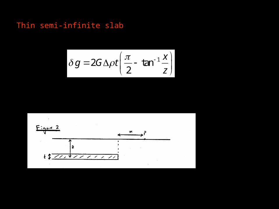
Thin semi-infinite slab

12 tan2

xg G t

z

12 tan2

xg G t

z

12 tan2

xg G t

z

12 tan2

xg G t

z

2g Gt

δg = 0

Change occurs more rapidly when slab is closer to the surface

Sets of theoretical curves are very useful

= 8.38 gu

Semi-infinite thick horizontal slab

12 2 1 1

2

2 1r

g G z z x nr

Start with a simple model – gradually make it more sophisticated

Modelling and non-uniquenessAn infinite number of subsurface density models will fit the gravity data equally as well

Can we constrain Δρ?

Can drill holes constrain parts of the model?

Do we have geological knowledge that limits therange of possible density models?

Do we have other geophysical data that can distinguish between density models?

Forward modelling (by nature is often subjective)Guess model, see if it fits the observed data, change model until it does fit the data

Forward modelling example

matics of crater formation

Younger, thinner Proterozoic crust is adjacent to with the thickened Archean craton, NE India

Modelling and non-uniqueness

Four models of Chicxulub (a,b,c from gravity, magnetic and borehole data)

Numerical modelling crater formation

Morgan et al., 2000

Collins et al., 2002

Forward modelling cont.

Debate on shape of stratigraphic uplift

Shape tells us about thekinematics of crater formation

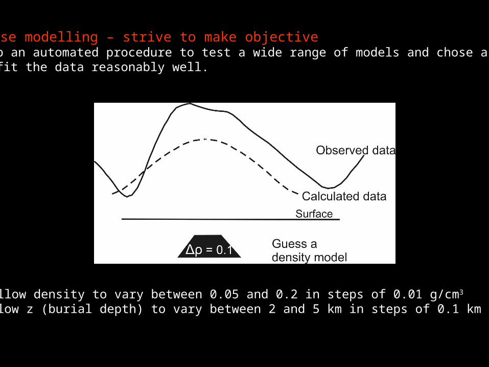
Inverse modelling – strive to make objectiveSet up an automated procedure to test a wide range of models and chose a range that fit the data reasonably well.

e.g. allow density to vary between 0.05 and 0.2 in steps of 0.01 g/cm3

and allow z (burial depth) to vary between 2 and 5 km in steps of 0.1 km

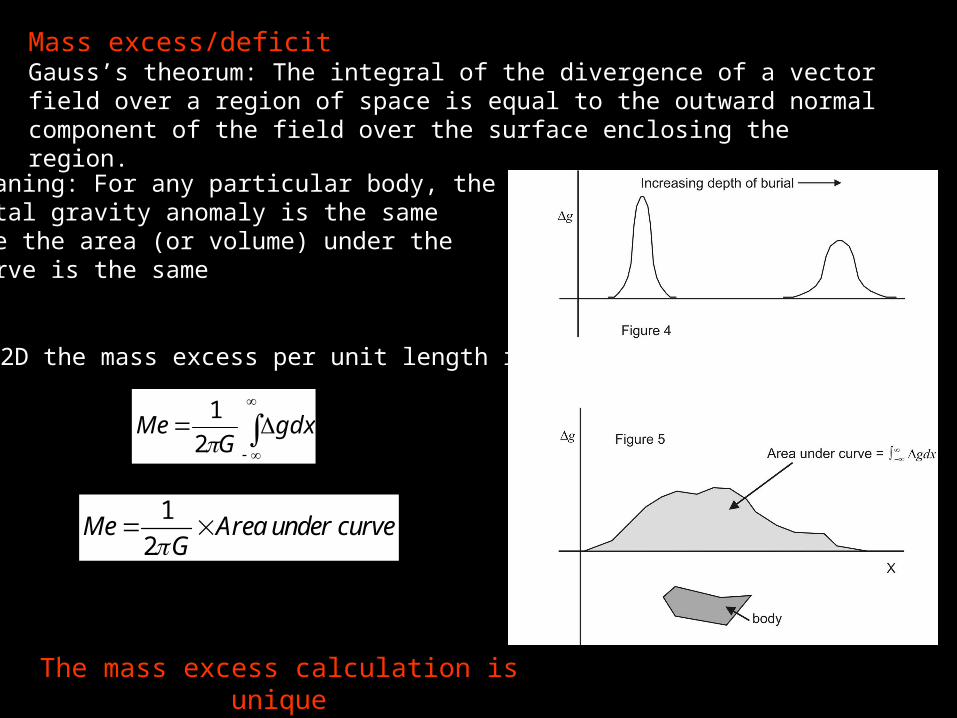
Mass excess/deficitGauss’s theorum: The integral of the divergence of a vector field over a region of space is equal to the outward normal component of the field over the surface enclosing the region.

gdxG

Me21

1

2Me Area under curve

G

The mass excess calculation is unique

Meaning: For any particular body, the total gravity anomaly is the samei.e the area (or volume) under the curve is the same

In 2D the mass excess per unit length is:

In 3D this would be:

gdxdyG

Me21 curveundervolume

GMe

21

Me = 1/2πG x ∑ Δg x Δa

where Δa is the area

∑ Δg = Δg1+ Δg2 + Δg3 ... etc

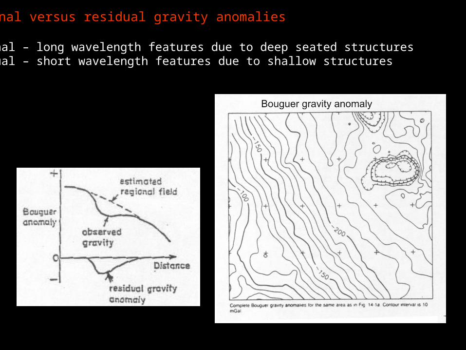
Regional versus residual gravity anomalies

Regional – long wavelength features due to deep seated structuresResidual – short wavelength features due to shallow structures

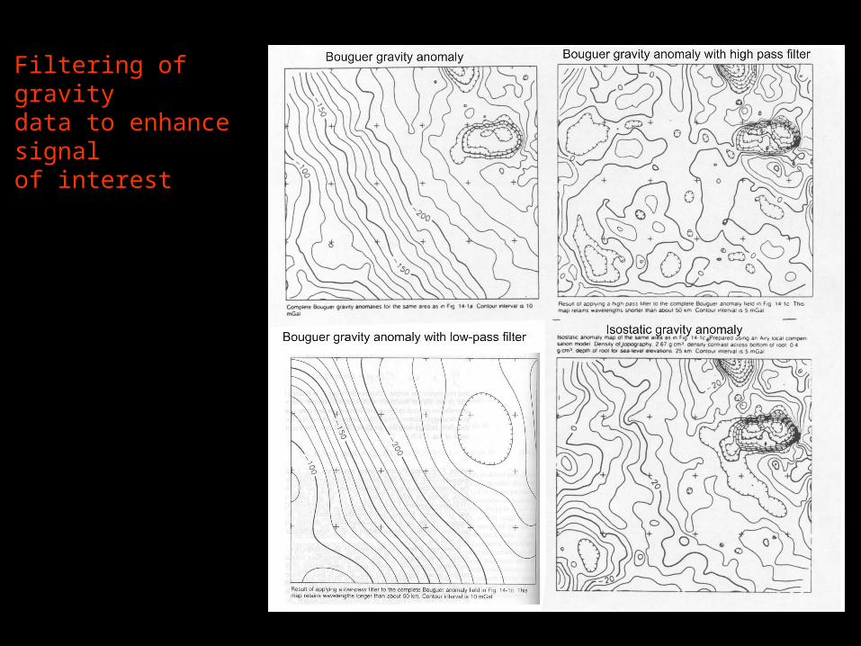
Filtering of gravity data to enhance signalof interest

z = 0

z = -s

z = s

z = 2s

We measure g on surface z = 0 at stations that are a distance x apart

We can calculate the value of g on any surface we like z = s, -s etc

gm = k1g0 + K2(g1+g-1) + K3(g2 + g-2)… etc

ki depends on s and x

g

gm

g0 g1 g2 g3g-1g-2

x

42

2

32

11

rr

g

rr

g

r

Gmg

The gradient of gravity data enhances the residual anomalies.

Bouguer gravity Horizontal gradient of Bouguer gravity