Probability Structure and Return Period of MultidayMonsoon Rainfall

Nur S. Muhammad1; Pierre Y. Julien, M.ASCE2; and Jose D. Salas, M.ASCE3

Abstract: The daily monsoon rainfall data recorded at Subang Airport, Malaysia, from 1960 to 2011 is examined in terms of probabilitystructure for the estimation of extreme daily rainfall precipitation during the Northeast (NE) and Southwest (SW) Malaysian monsoons. Thediscrete autoregressive and moving average [DARMA(1,1)] model is preferable to the first-order Markov chain [DAR(1)] model. The condi-tional probabilities of t consecutive rainy days are time dependent. Nevertheless, a simple two-parameter gamma distribution appropriatelyfits the frequency distribution of multiday rainfall amounts. An algorithm is developed by combining the DARMA(1,1) and gamma models toestimate the return period of multiday rainfall. Extensive comparisons showed that the DARMA(1,1)-gamma model gives a reliable estimateof the return period of rainfall for both NE and SW monsoons at Subang Airport. Furthermore, values generated from the models enable theanalysis of the frequency distribution of extreme rainfall events. DOI: 10.1061/(ASCE)HE.1943-5584.0001253. © 2015 American Societyof Civil Engineers.

Author keywords: Multiday rainfall; Monsoon rainfall precipitation; Return period; Conditional probability; Stochastic modeling.

Introduction

The planning and design of water resources projects require theanalysis of reliable, long-term hydrological data such as rainfalland streamflow. The stochastic point process was first introducedby Todorovic (1968) and subsequently used by Todorovic andYevjevich (1969) and Eagleson (1978) for modeling short-termrainfall. Kavvas and Delleur (1981) were successful in modelingthe sequence of daily rainfall in Indiana using the Neyman-Scott(NS) cluster process. They assumed that a rainfall event occursin midday, to comply with the model order. Multiday rainfall eventswere treated as a group instantaneous rainfall that occurs once aday, with a 1-day interval. Rodriguez-Iturbe et al. (1987) testedthe performance of different types of point process models, i.e., thePoisson and cluster-based models using hourly rainfall data fromDenver, Colorado. They concluded that the white-noise Poissonmodel was unable to produce satisfactory results. Instead,cluster-based models, namely the Neyman-Scott (NS) andBartlett-Lewis (BL) processes, are more flexible, reliable, and ableto represent the actual rainfall scenarios. Since then, other research-ers have improved the NS and BL processes to model fine-scalerainfall. Examples of the use of a modified BL model can be foundin Rodriguez-Iturbe et al. (1988), Glasbey et al. (1995), Khaliq andCunnane (1996), Cowpertwait et al. (2007), and Verhoest et al.(2010). In addition, Cowpertwait (1995), Cowpertwait et al.(1996), and Burton et al. (2008, 2010) are studies that utilize

the modified NS to model rainfall. However, Rodriguez-Iturbe et al.(1988), Cowpertwait et al. (1996, 2007), and Burton et al. (2008)show that the point-process models were unable to produce extremevalues with good accuracy. Furthermore, Obeysekera et al. (1987)applied various types of point-process models for hourly rainfallconsidering the diurnal cycle that is characteristic at certainlocations during some months of the year.

Low-order discrete autoregressive family models, such as thediscrete autoregressive [DAR(1)] and discrete autoregressive andmoving average [DARMA(1,1)] models, are frequently used forsimulating daily rainfall sequences. The DAR(1) model is alsoequivalent to a first-order Markov chain model. This model as-sumes that the probability of rain depends only on the current state(wet or dry) and will not be influenced by its past behavior. Haanet al. (1976), Katz (1977), Roldán and Woolhiser (1982), Small andMorgan (1986), Jimoh and Webster (1996), Sharma (1996), Tanand Sia (1997), and Wilks (1998) are among the studies that weresuccessful in modeling the sequence of rainy and dry days usingfirst-order Markov chains. Wilks (1998) used the first-orderMarkov chain to simulate the occurrence of daily rainfall basedon data from 1951 to 1996 from 25 stations in New York State,USA. The statistical properties such as the joint probabilities forboth rainy and dry days, mean monthly rainfall, and standard de-viations of monthly rainfall indicate that the simulated rainfall datareproduce the rainfall data statistics really well. It was concludedthat the model was successful in preserving the dependence natureof daily rainfall at these stations. First-order Markov chains are sim-ple and do not require a lot of computational effort. However,Feyerherm and Bark (1965) found that first-order Markov chainsare unable to model the scenario of strong dry day persistence.Similar findings were reported by Wallis and Griffiths (1995)and Semenov et al. (1998). The order of a Markov chain maybe influenced by seasonal change and location (Chin 1977;Cazacioc and Cipu 2005; Deni et al. 2009). Chin (1977) found thatthe seasonal change has a significant impact in determining thesuitable order of a Markov chain in more than 200 stations locatedthroughout the USA. High-order Markov chains are suitable tomodel the sequence of daily precipitation during winter at moststations, and first-order Markov chains are appropriate for summer.

1Lecturer, Dept. of Civil and Structural Engineering, Faculty ofEngineering and Built Environment, Universiti Kebangsaan Malaysia,Bangi, Selangor 43600, Malaysia (corresponding author). E-mail:shazwani.muhammad@ukm.edu.my

2Professor, Dept. of Civil and Environmental Engineering, ColoradoState Univ., Fort Collins, CO 80523.

3Professor Emeritus, Dept. of Civil and Environmental Engineering,Colorado State Univ., Fort Collins, CO 80523.

Note. This manuscript was submitted on August 2, 2013; approved onApril 21, 2015; published online on June 17, 2015. Discussion period openuntil November 17, 2015; separate discussions must be submitted forindividual papers. This paper is part of the Journal of Hydrologic Engi-neering, © ASCE, ISSN 1084-0699/04015048(11)/$25.00.

© ASCE 04015048-1 J. Hydrol. Eng.

J. Hydrol. Eng.

Dow

nloa

ded

from

asc

elib

rary

.org

by

Col

orad

o St

ate

Uni

v L

brs

on 0

9/18

/15.

Cop

yrig

ht A

SCE

. For

per

sona

l use

onl

y; a

ll ri

ghts

res

erve

d.

The physical environmental causes and geography can influencethe order of Markov chains. Similar findings were reported byCazacioc and Cipu (2005) for the simulation of rainfall sequencesat several stations in Romania.

For tropical regions, a different approach was used by Deniet al. (2009) in the analysis of Malaysian daily rainfall data basedon the Markov chain model. The objective of their study was tofind the optimum order of a Markov chain for daily rainfall duringthe Northeast (NE) and Southwest (SW) monsoons using two dif-ferent thresholds, i.e., 0.1 and 10.0 mm, where NE and SWare thedirections from which the monsoons are coming. The Akaikeinformation criteria (AIC) and Bayesian information criteria wereused to determine the appropriate order of the Markov chain mod-els. The study used the available data from 18 rainfall stationslocated in various parts of Peninsular Malaysia. They concludedthat the optimum order of a Markov chain varies with the location,monsoon season, and the level of threshold. For example, theoccurrence of rainfall (threshold level 10.0 mm) for the NEand SW monsoons at stations located in the northwestern andeastern regions of Peninsular Malaysia can be represented usinga first-order Markov chain. Additionally, higher order Markovchain models are suitable to represent rainfall occurrence,especially during the NE monsoon, for both levels of threshold.Other examples of the use of a high-order Markov chain tosimulate the rain and dry day sequence are reported by Mimikou(1983), Dahale et al. (1994), Katz and Parlange (1998), andDastidar et al. (2010).

Even though higher order Markov chain models may be used toovercome the lack of persistence of the simple Markov chain, moreparameters have to be used, which increases the model uncertainty(Jacobs and Lewis 1983) and also makes the calculations morecomplex. Jacobs and Lewis (1978) and Kedem (1980) discussthe concept of the stationary DARMA model, which is intendedto be simpler for modeling stationary sequences of dependentdiscrete random variables with specified marginal distributionand correlation structure. Buishand (1977, 1978) modeled thesequence of daily rainfall using DARMA(1,1) at several stationsin the Netherlands, Suriname, India, and Indonesia. SinceDARMA(1,1) is a stationary model, the data for each station weredivided into their respective seasons in order to consider the rainfallseasonal variations. The results have shown that the DARMA(1,1)model is successful in simulating the daily rainfall in tropical andmonsoon areas, where prolonged dry and wet seasons may occur.The DARMA(1,1) model provides longer persistence than theDAR(1) model does. Other studies that use the DARMA(1,1)model to simulate sequences of daily rainfall include Chang et al.(1982, 1984b, a), Delleur et al. (1989), and Cindric (2006). Inaddition, DARMA models have been applied for the analysis ofdroughts (Chung and Salas 2000; Salas et al. 2005; Cancelliereand Salas 2010). For example, Chung and Salas (2000) analyzedthe annual streamflow time series of the Niger River in Africa andconcluded that the drought occurrence can be successfullysimulated using the DARMA(1,1) model. The results showed longperiods of low flows (drought) and high flows, and the DARMA(1,1) model was suitable for simulating streamflows with a longermemory as compared to the DAR(1) model.

Return periods are useful in hydrology to measure the severityof an event. Various definitions of return period have been reportedin the literature, such as first arrival time and interarrival time orrecurrence interval. These definitions give different values whenthe events are dependent in time. However, for single and indepen-dent events, the first arrival time and recurrence interval give thesame value (Fernández and Salas 1999a). Extensive theoriesand applications on the return period definitions and serial

dependence are discussed in Fernández and Salas (1999a, b).Woodyer et al. (1972), Kite (1978), Lloyd (1970), Loaiciga andMariňo (1991), and Şen (1999) defined recurrence interval asthe average elapsed time between the occurrences of critical events,such as earthquakes of high magnitude and extreme floods ordroughts. In addition, Vogel (1987) and Douglas et al. (2002) usedthe return period as the average number of trials required to the firstoccurrence of a critical event. This definition may be more useful inrelation to reservoir operation because knowing the first time thatthe reservoir is at risk of failure is of greater interest than the aver-age time between failures (Douglas et al. 2002). Furthermore, Goelet al. (1998), Shiau and Shen (2001), Kim et al. (2003), Gonzálezand Valdéz (2003), Salas et al. (2005), and Cancelliere and Salas(2004, 2010) reported studies on the calculation of return periodand risk that include both the amount and duration of extremehydrological events.

This study concentrates on the occurrence of multiday rainfallevents in Malaysia. The country experiences two major seasonsclassified as the Northeast (NE) and Southwest (SW) monsoons.The NE monsoon typically occurs from November to March, whilethe SW monsoon is from May to September. April and October areknown as intermonsoon months. Both monsoons bring lots ofmoisture and as a result, Malaysia receives between 2,000 to4,000 mm of rainfall with 150 to 200 rainy days annually (Suhailaand Jemain 2007). One of the most devastating recent multidayrainfall events resulted in the Kota Tinggi flood in December2006 and January 2007. These two extreme monsoon events re-sulted in more than 350 and 450 mm of cumulative rainfall in lessthan a week. The estimated economic loss reached half a billion USdollars and more than 100,000 local residents had to be evacuated(Abu Bakar et al. 2007). Even though it is well known that multidayevents are the main cause of flooding in Malaysia, the topic hasreceived little attention from local researchers.

This paper discusses various aspects of Malaysian monsoons,including the probability distribution and probability structure ofmultiday monsoon rainfall events, the modeling and simulationof daily rainfall sequences, the estimation of extreme rainfall quan-tiles, and the estimation of the return period of multiday rainfall.The occurrences of daily rainfall are characterized and simulatedusing the discrete autoregressive and moving average [DARMA(1,1)] model. These approaches were tested using the observeddaily rainfall measurements collected from Subang Airport nearKuala Lumpur, Malaysia.

Summary of DAR(1) and DARMA(1,1) Models

This study uses the DAR(1) and DARMA(1,1) models to simulatethe occurrence of daily rainfall. The DAR(1) model is representedas (Jacobs and Lewis 1978)

At ¼ VtAt−1 þ ð1 − VtÞYt

with At ¼�At−1 with probability λ

Yt with probability ð1 − λÞ ð1Þ

where Vt is an independent random variable taking values of 0 and1 such that

PðVt ¼ 1Þ ¼ λ ¼ 1 − PðVt ¼ 0Þ ð2Þand λ is a parameter. The variable Yt is another independent andidentically distributed (i.i.d.) random variable, with a commonprobability πk ¼ PðYt ¼ kÞ; k ¼ 0,1.

It should be noted that At is a first-order Markov chainand the process of simulation is assumed to start at A−1

© ASCE 04015048-2 J. Hydrol. Eng.

J. Hydrol. Eng.

Dow

nloa

ded

from

asc

elib

rary

.org

by

Col

orad

o St

ate

Uni

v L

brs

on 0

9/18

/15.

Cop

yrig

ht A

SCE

. For

per

sona

l use

onl

y; a

ll ri

ghts

res

erve

d.

(Buishand 1978). The autocorrelation function of the DAR(1)model is (Jacobs and Lewis 1978)

corrðAt;At−kÞ ¼ rkðAÞ ¼ λk; k ≥ 1 ð3Þwhere rk is the lag-k (days) autocorrelation function.

The autocorrelation function ðrkÞ is estimated based on the se-quences of dry and rainy days, i.e., 0 s and 1 s, and not the rainfallamounts (Delleur et al. 1989) as

rk ¼"XN−k

t¼1

ðxt − xÞðxtþk − xÞ#"XN

t¼1

ðxt − xÞ2#−1

ð4Þ

x ¼ 1

N

XNt¼1

xt ð5Þ

where rk is the lag-k autocorrelation coefficient and N is thesample size.

There are two parameters associated with the DAR(1) model,i.e., π0 (or π1) and λ. The parameter λ may be estimated fromthe lag-1 autocorrelation coefficient as given in Eqs. (3) and (4).The parameters π0 and π1 are based on the dry and wet run lengthsthat are obtained from the observed daily rainfall data set. They areestimated using Eqs. (6) and (7) (Buishand 1978) as follows:

π0 ¼T0

T0 þ T1

ð6Þ

π1 ¼ 1 − π0 ð7Þwhere T0 = mean run length for dry days and T1 = mean run lengthfor wet days.

The one-step transitional probability, pði; jÞ ¼ PðAtþ1 ¼jjAt ¼ iÞ is given by (Jacobs and Lewis 1978) as follows:

pði; jÞ ¼�λþ ð1 − λÞπj; ifi ¼ jð1 − λÞπj; ifi ≠ j i; j ¼ 0; 1 ð8Þ

Eq. (8) can also be represented in terms of the transitionalprobability matrix, as shown in Eq. (9)

P ¼�λþ ð1 − λÞπ0 ð1 − λÞπ1

ð1 − λÞπ0 λþ ð1 − λÞπ1

�ð9Þ

The transitional probability matrix simplifies the calculation ofrun length. The concept of run length is important, especially in mod-eling the sequence of daily rainfall. The run length is defined as thesuccession of events of the same kind, and it is bounded at the begin-ning and the end by events of a different kind. For the DAR(1) model,the probability distribution of wet and dry run lengths can be ob-tained from Eqs. (10) and (11) as derived by Chang et al. (1984b)

PðT1 ¼ nÞ ¼ pn−1ð1; 1Þ½1 − pð1; 1Þ� ð10Þ

PðT0 ¼ nÞ ¼ pn−1ð0; 0Þ½1 − pð0; 0Þ� ð11Þ

The DARMA(1,1) model is represented as (Jacobs and Lewis1978)

Xt ¼ UtYt þ ð1 − UtÞAt−1

with Xt ¼�Yt with probability β

At−1 with probabilityð1 − βÞ ð12Þ

where Ut is an independent random variable taking values of 0 or 1only such that

PðUt ¼ 1Þ ¼ β ¼ 1 − PðUt ¼ 0Þ ð13Þ

Yt is another i.i.d. random variable having a commonprobability πk ¼ PðYt ¼ kÞ, k ¼ 0,1, and At is an autoregressivecomponent given by

At ¼�At−1 with probability λYt with probability ð1 − λÞ

The variable At has the same probability distribution as Yt but isindependent of Yt. It should be noted that Xt is not Markovian, butðXt;AtÞ forms a first-order bivariate Markov chain.

The autocorrelation function of the DARMA(1,1) model is(Buishand 1978)

corrðXt;Xt−kÞ ¼ rkðXÞ ¼ cλk−1; k ≥ 1 ð14Þ

where c ¼ ð1 − βÞðβ þ λ − 2λβÞ ð15Þ

The three parameters of the DARMA(1,1) model need to beestimated, namely π0 or π1, λ, and β. The parameters π0 or π1

may be estimated from Eqs. (6) to (7). The estimation of λ maybe determined by minimizing Eq. (16) using the Newton-Raphsoniteration techniques. Buishand (1978) suggested using the ratio ofthe second to the first autocorrelation coefficients as an initialestimate for λ, as shown in Eq. (17)

ϕðλÞ ¼XMk¼1

½rk − cλk−1�2; k ≥ 1 ð16Þ

λ ¼ r2r1

ð17Þ

in whichM is the total number of lags considered, c can determinedfrom the lag-1 autocorrelation coefficient of the DARMA(1,1)model, and β can be estimated from Eq. (18)

β ¼ð3λ − 1Þ �

ffiffiffiffiffiffiffiffiffiffiffiffiffiffiffiffiffiffiffiffiffiffiffiffiffiffiffiffiffiffiffiffiffiffiffiffiffiffiffiffiffiffiffiffiffiffiffiffiffiffiffiffiffiffiffiffiffiffið3λ − 1Þ2 − 4ð2λ − 1Þðλ − cÞ

q2ð2λ − 1Þ ð18Þ

The probability distributions of the wet and dry run lengthsfor the DARMA(1,1) model are well known in the literature(e.g., Jacobs and Lewis 1978), see the Appendix for more details.

Probability Distribution and Return Period of MultidayRainfall Events

In this section, the probability distribution and return period formultiday rainfall events are investigated considering that theoccurrence of daily rainfall is correlated. The return period of multi-day rainfall events is based on the number of trials between twosuccessive occurrences of the same event. Multiday rainfall eventsoccur frequently during the NE and SW monsoons. Therefore, it isappropriate to estimate the return period as the average time(in days) between the occurrences of specific events. It may alsobe referred to as the recurrence interval. The most importantparameters that hydrologists and water resources specialists areconcerned about when analyzing a multiday rainfall event arethe duration and the amount of cumulative rainfall. Hence, thisstudy considers both parameters in formulating the estimation ofthe return period.

© ASCE 04015048-3 J. Hydrol. Eng.

J. Hydrol. Eng.

Dow

nloa

ded

from

asc

elib

rary

.org

by

Col

orad

o St

ate

Uni

v L

brs

on 0

9/18

/15.

Cop

yrig

ht A

SCE

. For

per

sona

l use

onl

y; a

ll ri

ghts

res

erve

d.

Muhammad (2013) found that the two-parameter gamma func-tion is most suitable for representing the rainfall amount distribu-tion for specified durations at Subang Airport. The method ofmoments is used to estimate the parameters and the formulascan be found in Mood et al. (1974) or Yevjevich (1984). It shouldbe noted that (e.g., Mood et al. 1974) if two independent gammavariables are added, for example, X ¼ R1 þ R2 where both R1 andR2 are gamma(α, β), then X is also gamma(α, 2β). Likewise, if youadd t independent gamma(α, β) variables then X ¼ R1þR2 þ : : : þ Rt is gamma(α, tβ). The data analysis showed thatthe two-parameter gamma distribution was best for describingthe distribution of 1-day and multiday rainfall events at SubangAirport. The empirical representation of rainfall amount distribu-tion in t consecutive rainy days is given in Eq. (19)

fðxÞ ≅ 1

j24.0jΓð0.6tÞ�

x24.0

�0.6 t−1

exp

�− x24.0

�ð19Þ

where x = total amount of rainfall for t consecutive rainy days (mm)and t = number of consecutive rainy days.

Thus, for a given rainfall duration, t, Eq. (19) enables one todetermine the probability of any rainfall event exceeding say x0. De-noting such a probability as PðEjtÞ, it may be determined as follows:

PðEjtÞ ¼Z∞x0

fðxÞdx ð20Þ

To determine the return period of rainfall events, E, of a givenduration, t, an approach used previously for determining the returnperiod of droughts (e.g., Cancelliere and Salas 2002; Gonzáles andValdés 2003; Salas et al. 2005) were followed. It follows that thereturn period of multiday rainfall events can be determined as

T ¼ T1 þ T0

PðEjtÞ ð21Þ

where T1 = mean run length for wet days; T0 = mean run length fordry days; and PðEjtÞ = probability of a rainfall event givenby Eq. (20).

Results and Discussion

Probability Distribution of Daily Rainfall

The daily rainfall measurements at Subang Airport (3°7′1.20″N,101°33′0.00″E) were used in this study. A long and reliable recordof 52 years for the period 1960 to 2011 was provided by theDepartment of Meteorology, Malaysia.

Fig. 1 shows the cumulative distribution function (CDF) for1-day and multiday rainfall at Subang Airport. The figure showsthat the two-parameter gamma distribution function given byEq. (19) fits reasonably well the historical CDF for 1 through 6 daysof rainfall duration. The CDF plot shows that for a single rainy day,there is about 60% chance that the rainfall amount will be less than10 mm, and there is a less than 5% chance that the rainfall amountwill exceed 50 mm. The multiday rainfall events resulted in asignificant amount of rainfall to the study area. The CDF plot alsoshows that there is a nonnegligible probability that 2 and 3 consecu-tive rainy days may produce more than 100 mm of rain. Further,there is 50% of chance of 4, 5, and 6 consecutive rainy daysyielding more than 55, 65, and 85 mm of rainfall, respectively.The probability of rainfall events with more than 100 mm of rainincreases as the number of consecutive rainy days increases. These

results illustrate the important need for a detailed analysis of bothduration and magnitude of multiday rainfall events.

Probability Structure of Rainfall Occurrence

When rain occurs on a given day, it is called a wet day while theabsence of rain on a given day is called a dry day. In this study, awet day is indicated for rainfall amounts of more than 0.1 mm,while a dry day is assumed for amounts less than or equal to0.1 mm. The threshold amount was determined based on the VonNeumann (1941) ratio and a more detailed analysis is presented inMuhammad (2013).

The analysis of the probability structure of rainfall events atSubang Airport shows that more than 50% of the events observedat the study site are rainy days. The estimated probability of rain onany given day is 0.53. If day-to-day rainfall events were indepen-dent, the probability of rain on any day would remain constant at0.53 [shown by a triangle in Fig. 2(a)]. However, Fig. 2(a) showsthat the field rainfall measurements of the conditional probabilityincreases significantly as the number of consecutive rainy day in-creases, i.e., from 0.53 for a single rainy day to about 0.80 for 15consecutive rainy days. For example, the estimated conditionalprobability of a fourth rainy day, given that it follows 3 consecutiverainy days, is 0.68. This probability is far greater than the estimatedprobability of the first day of rain, i.e., 0.53. The occurrence of rainon a given day affects the probability of rain the following days.Thus, the conditional probabilities estimated from the historicaldata show that the events are dependent.

Likewise, Fig. 2(b) gives the estimated conditional probabilitiesof n consecutive dry days at Subang Airport. The estimatedprobability that any given day is dry is 0.47, which increasessignificantly to 0.72 after 15 consecutive dry days. For example,the estimated conditional probability for a second consecutivedry day is 0.58, and the estimated probability for the third dryday increases to 0.63. Thus, the probability structure of n consecu-tive dry days is also dependent as is the case for rainy days. Table 1gives the details of the frequency and the estimated conditionalprobabilities of 1 to 15 consecutive wet and dry days.

Modeling the Occurrence of Daily Rainfall

In this study, the NE and SW monsoons are considered as the dailyrainfall recorded during the months of October to March and April

0.0

0.1

0.2

0.3

0.4

0.5

0.6

0.7

0.8

0.9

1.0

0 10 20 30 40 50 60 70 80 90 100 110 120 130 140 150

F(x)

Rainfall, x (mm)

1-day 2-days 3-days 4-days 5-days 6-days

1-day 2-days 3-days 4-days 5-days 6-days

Observed Theoretical

Rainy days

1 ra

iny

day

2 co

nsec

utiv

e rain

y da

ys

3 co

nsec

utiv

e rain

y da

ys

5 con

secu

tive r

ainy d

ays

6 con

secu

tive r

ainy d

ays

4 co

nsec

utiv

e rain

y da

ys

Fig. 1. Cumulative distribution function of 1-day and multiday rainfallevents at Subang Airport

© ASCE 04015048-4 J. Hydrol. Eng.

J. Hydrol. Eng.

Dow

nloa

ded

from

asc

elib

rary

.org

by

Col

orad

o St

ate

Uni

v L

brs

on 0

9/18

/15.

Cop

yrig

ht A

SCE

. For

per

sona

l use

onl

y; a

ll ri

ghts

res

erve

d.

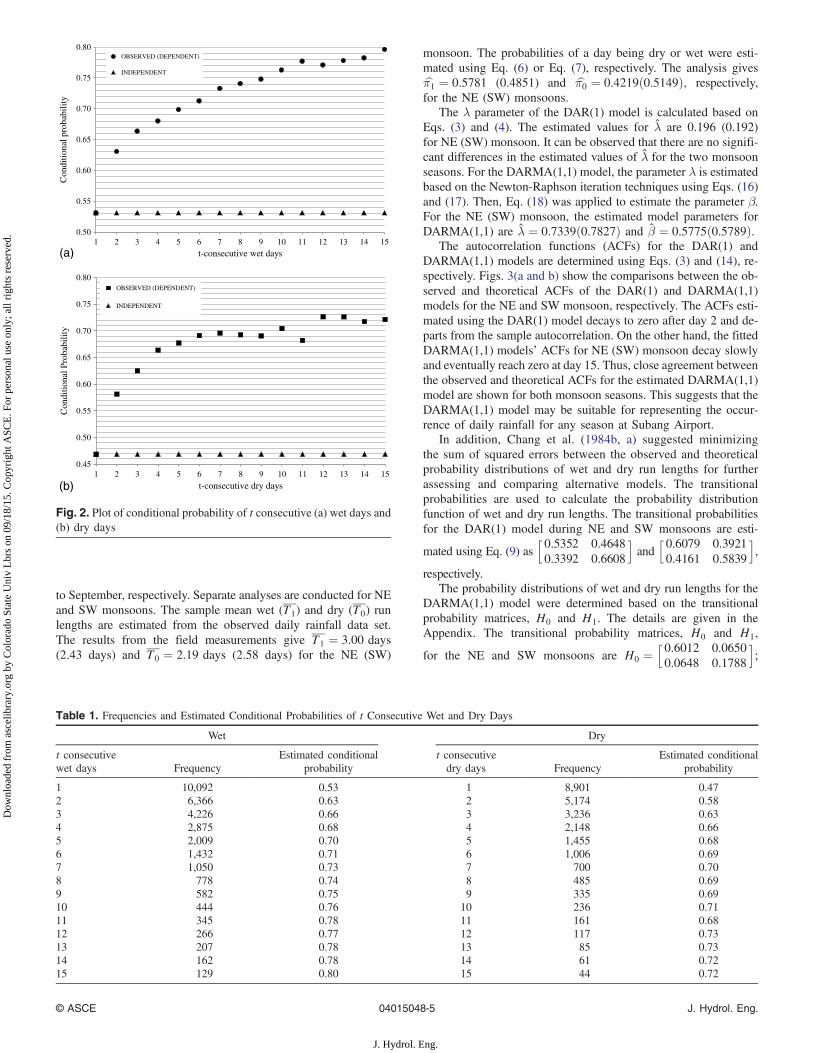
to September, respectively. Separate analyses are conducted for NEand SW monsoons. The sample mean wet (T1) and dry (T0) runlengths are estimated from the observed daily rainfall data set.The results from the field measurements give T1 ¼ 3.00 days(2.43 days) and T0 ¼ 2.19 days (2.58 days) for the NE (SW)

monsoon. The probabilities of a day being dry or wet were esti-mated using Eq. (6) or Eq. (7), respectively. The analysis givesbπ1 ¼ 0.5781 (0.4851) and bπ0 ¼ 0.4219ð0.5149Þ; respectively,for the NE (SW) monsoons.

The λ parameter of the DAR(1) model is calculated based onEqs. (3) and (4). The estimated values for λ are 0.196 (0.192)for NE (SW) monsoon. It can be observed that there are no signifi-cant differences in the estimated values of λ for the two monsoonseasons. For the DARMA(1,1) model, the parameter λ is estimatedbased on the Newton-Raphson iteration techniques using Eqs. (16)and (17). Then, Eq. (18) was applied to estimate the parameter β.For the NE (SW) monsoon, the estimated model parameters forDARMA(1,1) are λ ¼ 0.7339ð0.7827Þ and β ¼ 0.5775ð0.5789Þ.

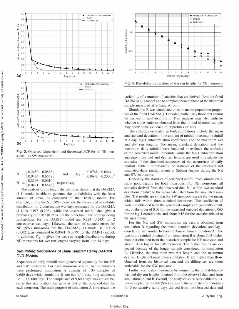
The autocorrelation functions (ACFs) for the DAR(1) andDARMA(1,1) models are determined using Eqs. (3) and (14), re-spectively. Figs. 3(a and b) show the comparisons between the ob-served and theoretical ACFs of the DAR(1) and DARMA(1,1)models for the NE and SW monsoon, respectively. The ACFs esti-mated using the DAR(1) model decays to zero after day 2 and de-parts from the sample autocorrelation. On the other hand, the fittedDARMA(1,1) models’ ACFs for NE (SW) monsoon decay slowlyand eventually reach zero at day 15. Thus, close agreement betweenthe observed and theoretical ACFs for the estimated DARMA(1,1)model are shown for both monsoon seasons. This suggests that theDARMA(1,1) model may be suitable for representing the occur-rence of daily rainfall for any season at Subang Airport.

In addition, Chang et al. (1984b, a) suggested minimizingthe sum of squared errors between the observed and theoreticalprobability distributions of wet and dry run lengths for furtherassessing and comparing alternative models. The transitionalprobabilities are used to calculate the probability distributionfunction of wet and dry run lengths. The transitional probabilitiesfor the DAR(1) model during NE and SW monsoons are esti-

mated using Eq. (9) ash0.5352 0.46480.3392 0.6608

iand

h0.6079 0.39210.4161 0.5839

i,

respectively.The probability distributions of wet and dry run lengths for the

DARMA(1,1) model were determined based on the transitionalprobability matrices, H0 and H1. The details are given in theAppendix. The transitional probability matrices, H0 and H1,

for the NE and SW monsoons are H0 ¼h0.6012 0.06500.0648 0.1788

i;

0.50

0.55

0.60

0.65

0.70

0.75

0.80

1 2 3 4 5 6 7 8 9 10 11 12 13 14 15

ytilibaborp lanoitidnoC

t-consecutive wet days

OBSERVED (DEPENDENT)

INDEPENDENT

0.45

0.50

0.55

0.60

0.65

0.70

0.75

0.80

1 2 3 4 5 6 7 8 9 10 11 12 13 14 15

ytilibaborP lanoitidno

C

t-consecutive dry days

OBSERVED (DEPENDENT)

INDEPENDENT

(a)

(b)

Fig. 2. Plot of conditional probability of t consecutive (a) wet days and(b) dry days

Table 1. Frequencies and Estimated Conditional Probabilities of t Consecutive Wet and Dry Days

Wet Dry

t consecutivewet days Frequency

Estimated conditionalprobability

t consecutivedry days Frequency

Estimated conditionalprobability

1 10,092 0.53 1 8,901 0.472 6,366 0.63 2 5,174 0.583 4,226 0.66 3 3,236 0.634 2,875 0.68 4 2,148 0.665 2,009 0.70 5 1,455 0.686 1,432 0.71 6 1,006 0.697 1,050 0.73 7 700 0.708 778 0.74 8 485 0.699 582 0.75 9 335 0.6910 444 0.76 10 236 0.7111 345 0.78 11 161 0.6812 266 0.77 12 117 0.7313 207 0.78 13 85 0.7314 162 0.78 14 61 0.7215 129 0.80 15 44 0.72

© ASCE 04015048-5 J. Hydrol. Eng.

J. Hydrol. Eng.

Dow

nloa

ded

from

asc

elib

rary

.org

by

Col

orad

o St

ate

Uni

v L

brs

on 0

9/18

/15.

Cop

yrig

ht A

SCE

. For

per

sona

l use

onl

y; a

ll ri

ghts

res

erve

d.

H1 ¼h0.2450 0.08880.0474 0.6548

iand H0 ¼

h0.6748 0.04440.0648 0.2333

i;

H1 ¼h0.2198 0.06100.0471 0.6548

i, respectively.

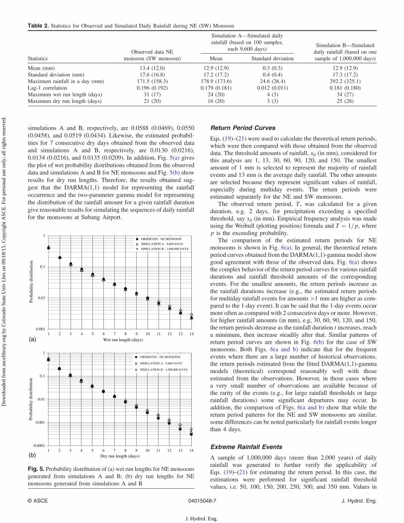
The analysis of run length distributions shows that the DARMA(1,1) model is able to generate the probabilities with the leastamount of error, as compared to the DAR(1) model. Forexample, during the NE (SW) monsoon, the theoretical probabilitydistribution for 2 consecutive wet days estimated for the DARMA(1,1) is 0.197 (0.206), while the observed rainfall data give aprobability of 0.207 (0.218). On the other hand, the correspondingprobabilities for the DAR(1) model are 0.224 (0.243) for 2consecutive wet days. Likewise, the sum of squared errors forNE (SW) monsoons for the DARMA(1,1) model is 0.0015(0.0021), as compared to 0.0091 (0.0079) for the DAR(1) model.In addition, Fig. 4 gives the wet run length distributions duringNE monsoons for wet run lengths varying from 1 to 14 days.

Simulating Sequences of Daily Rainfall Using DARMA(1,1) Models

Sequences of daily rainfall were generated separately for the NEand SW monsoons. For each monsoon season, two simulationswere performed; simulation A consists of 100 samples of9,600 days while simulation B consists of a very long sequence,i.e. 1,000,000 days. The sample size of 9,600 days was chosen be-cause this size is about the same as that of the observed data foreach monsoon. The main purpose of simulation A is to assess the

variability of a number of statistics that are derived from the fittedDARMA(1,1) model and to compare them to those of the historicalsample measured at Subang Airport.

Simulation B was conducted to estimate the population proper-ties of the fitted DARMA(1,1) model, particularly those that cannotbe derived in analytical form. This analysis may also indicatewhether some statistics obtained from the limited historical samplemay show some evidence of departures or bias.

The statistics estimated in both simulations include the meanand standard deviation of the amount of rainfall, maximum rainfallin a day, lag-1 autocorrelation coefficient, and the maximum wetand dry run lengths. The mean, standard deviation, and themaximum daily rainfall were included to evaluate the statisticsof the generated rainfall amounts, while the lag-1 autocorrelationand maximum wet and dry run lengths are used to evaluate thestatistics of the simulated sequences of the occurrence of dailyrainfall. Table 2 summarizes the statistics of the observed andsimulated daily rainfall events at Subang Airport during the NEand SW monsoons.

Generally, the statistics of generated rainfall from simulation Ashow good results for both monsoons. For NE monsoons, allstatistics derived from the observed data fall within two standarddeviations relative to the mean calculated from the simulated sam-ples. The results are similar for SW monsoon except for the mean,which falls within three standard deviations. The coefficient ofvariation obtained from the generated samples are generally small,i.e., on the order of 0.02 for the mean and standard deviation, 0.065for the lag-1 correlations, and about 0.16 for the statistics related tothe maximums.

For the NE and SW monsoons, the results obtained fromsimulation B regarding the mean, standard deviation, and lag-1correlation are similar to those obtained from simulation A. Themaximum rainfall obtained from simulation B is about 70% higherthan that obtained from the historical sample for NE monsoon andabout 100% higher for SW monsoon. The higher results are ex-pected because of the longer sample considered for simulationB. Likewise, the maximum wet run length and the maximumdry run length obtained from simulation B are higher than thoseobtained from the historical data and the differences are morenoticeable for the SW monsoon.

Further verification was made by comparing the probabilities ofwet and dry run lengths obtained from the observed data and fromsimulations A and B. Overall, the analyses show reasonable results.For example, for the NE (SW) monsoon the estimated probabilitiesfor 5 consecutive rainy days derived from the observed data and

0.0

(a)

(b)

0.1

0.2

0.3

0.4

0.5

0.6

0.7

0.8

0.9

1.0

0 1 2 3 4 5 6 7 8 9 10 11 12 13 14 15

Aut

o-)F

CA( noitcnuf noitalerroc

Lag (day)

OBSERVED - NE MONSOON

DAR(1)

DARMA(1,1)

0.0

0.1

0.2

0.3

0.4

0.5

0.6

0.7

0.8

0.9

1.0

0 1 2 3 4 5 6 7 8 9 10 11 12 13 14 15

Aut

o-)F

CA( noitcnuf noitalerroc

Lag (day)

OBSERVED - SW MONSOON

DAR(1)

DARMA(1,1)

Fig. 3. Observed (dependent) and theoretical ACF for (a) NE mon-soons; (b) SW monsoons

0.001

0.01

0.1

1

1 2 3 4 5 6 7 8 9 10 11 12 13 14

noitubirtsidytilibabor

P

Wet run length (days)

OBSERVED - NE MONSOON

DAR(1)

DARMA(1,1)

Fig. 4. Probability distribution of wet run lengths for NE monsoons

© ASCE 04015048-6 J. Hydrol. Eng.

J. Hydrol. Eng.

Dow

nloa

ded

from

asc

elib

rary

.org

by

Col

orad

o St

ate

Uni

v L

brs

on 0

9/18

/15.

Cop

yrig

ht A

SCE

. For

per

sona

l use

onl

y; a

ll ri

ghts

res

erve

d.

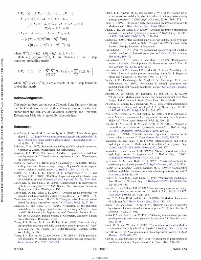
simulations A and B, respectively, are 0.0588 (0.0469), 0.0550(0.0458), and 0.0519 (0.0434). Likewise, the estimated probabil-ities for 7 consecutive dry days obtained from the observed dataand simulations A and B, respectively, are 0.0130 (0.0216),0.0134 (0.0216), and 0.0135 (0.0209). In addition, Fig. 5(a) givesthe plot of wet probability distributions obtained from the observeddata and simulations A and B for NE monsoons and Fig. 5(b) showresults for dry run lengths. Therefore, the results obtained sug-gest that the DARMA(1,1) model for representing the rainfalloccurrence and the two-parameter gamma model for representingthe distribution of the rainfall amount for a given rainfall durationgive reasonable results for simulating the sequences of daily rainfallfor the monsoons at Subang Airport.

Return Period Curves

Eqs. (19)–(21) were used to calculate the theoretical return periods,which were then compared with those obtained from the observeddata. The threshold amounts of rainfall, x0 (in mm), considered forthis analysis are 1, 13, 30, 60, 90, 120, and 150. The smallestamount of 1 mm is selected to represent the majority of rainfallevents and 13 mm is the average daily rainfall. The other amountsare selected because they represent significant values of rainfall,especially during multiday events. The return periods wereestimated separately for the NE and SW monsoons.

The observed return period, T, was calculated for a givenduration, e.g. 2 days, for precipitation exceeding a specifiedthreshold, say x0 (in mm). Empirical frequency analysis was madeusing the Weibull (plotting position) formula and T ¼ 1=p, wherep is the exceeding probability.

The comparison of the estimated return periods for NEmonsoons is shown in Fig. 6(a). In general, the theoretical returnperiod curves obtained from the DARMA(1,1)-gamma model showgood agreement with those of the observed data. Fig. 6(a) showsthe complex behavior of the return period curves for various rainfalldurations and rainfall threshold amounts of the correspondingevents. For the smallest amounts, the return periods increase asthe rainfall durations increase (e.g., the estimated return periodsfor multiday rainfall events for amounts >1 mm are higher as com-pared to the 1-day event). It can be said that the 1-day events occurmore often as compared with 2 consecutive days or more. However,for higher rainfall amounts (in mm), e.g, 30, 60, 90, 120, and 150,the return periods decrease as the rainfall duration t increases, reacha minimum, then increase steadily after that. Similar patterns ofreturn period curves are shown in Fig. 6(b) for the case of SWmonsoons. Both Figs. 6(a and b) indicate that for the frequentevents where there are a large number of historical observations,the return periods estimated from the fitted DARMA(1,1)-gammamodels (theoretical) correspond reasonably well with thoseestimated from the observations. However, in those cases wherea very small number of observations are available because ofthe rarity of the events (e.g., for large rainfall thresholds or largerainfall durations) some significant departures may occur. Inaddition, the comparison of Figs. 6(a and b) show that while thereturn period patterns for the NE and SW monsoons are similar,some differences can be noted particularly for rainfall events longerthan 4 days.

Extreme Rainfall Events

A sample of 1,000,000 days (more than 2,000 years) of dailyrainfall was generated to further verify the applicability ofEqs. (19)–(21) for estimating the return period. In this case, theestimations were performed for significant rainfall thresholdvalues, i.e. 50, 100, 150, 200, 250, 300, and 350 mm. Values in

Table 2. Statistics for Observed and Simulated Daily Rainfall during NE (SW) Monsoon

StatisticsObserved data NE

monsoon (SW monsoon)

Simulation A—Simulated dailyrainfall (based on 100 samples,

each 9,600 days)Simulation B—Simulateddaily rainfall (based on onesample of 1,000,000 days)Mean Standard deviation

Mean (mm) 13.4 (12.0) 12.9 (12.9) 0.3 (0.3) 12.9 (12.9)Standard deviation (mm) 17.6 (16.8) 17.2 (17.2) 0.4 (0.4) 17.3 (17.2)Maximum rainfall in a day (mm) 171.5 (158.3) 178.9 (173.6) 24.6 (26.4) 292.2 (325.1)Lag-1 correlation 0.196 (0.192) 0.179 (0.181) 0.012 (0.011) 0.181 (0.180)Maximum wet run length (days) 31 (17) 24 (20) 4 (3) 34 (27)Maximum dry run length (days) 21 (20) 16 (20) 3 (3) 25 (28)

0.001

0.01

0.1

1

1 2 3 4 5 6 7 8 9 10 11 12 13 14

noitubirtsidytilibabor

P

Wet run length (days)

OBSERVED - NE MONSOON

SIMULATION A - 9,600 DAYS

SIMULATION B - 1,000,000 DAYS

0.0001

0.001

0.01

0.1

1

1 2 3 4 5 6 7 8 9 10 11 12 13 14

noitubirtsidytilibaborP

Dry run length (days)

OBSERVED - NE MONSOON

SIMULATION A - 9,600 DAYS

SIMULATION B - 1,000,000 DAYS

(a)

(b)

Fig. 5. Probability distribution of (a) wet run lengths for NE monsoonsgenerated from simulations A and B; (b) dry run lengths for NEmonsoons generated from simulations A and B

© ASCE 04015048-7 J. Hydrol. Eng.

J. Hydrol. Eng.

Dow

nloa

ded

from

asc

elib

rary

.org

by

Col

orad

o St

ate

Uni

v L

brs

on 0

9/18

/15.

Cop

yrig

ht A

SCE

. For

per

sona

l use

onl

y; a

ll ri

ghts

res

erve

d.

excess of 150 mm are considered to represent extreme to rare eventsand can cause devastating floods on large watersheds.

Fig. 7 shows the comparison between calculated return periodsbased on the generated sample and the theoretical equationscorresponding to NE monsoons. The 2,000-year rainfall wasgenerated using the fitted DARMA(1,1)-gamma models as de-scribed earlier. Generally, the return period curves for most rainfall

threshold amounts show excellent agreement, which further verifiesthat Eqs. (19)–(21) are reliable to estimate the return periods formultiday events. Some departures are noted for the very extremeamounts, i.e. 300 and 350 mm, which is attributed to the variabilityof the generated samples.

Furthermore, it was desired to illustrate the applicability of thefitted DARMA(1,1)-gamma models for obtaining via stochasticrainfall generation the variability of the T-year rainfall quantiles,i.e., the annual frequency distribution of the maximum daily rainfallat Subang Airport. Fig. 8 shows the computed annual frequencydistribution of maximum daily rainfall obtained from the 52-yearhistorical records and from the 100 samples of 2,000 years of rain-fall derived from the generated daily rainfall based on the fittedDARMA(1,1)-gamma models. This result may be particularly use-ful in cases of short records that may be available at a given sitewhere the occurrence of daily rainfall and the variability of rainfallamount can be modeled using the procedures described in this pa-per and the variability of the annual frequency distribution obtainedbased on data generation.

Summary and Conclusions

The analysis of both the Northeast (NE) and Southwest (SW) mon-soon rainfall precipitation events at Subang Airport in Malaysiafrom 1960–2011 demonstrates the following:1. The majority (57%) of rainfall events are multiday events;2. The distribution of daily rainfall is well reproduced (Fig. 1)

with a gamma distribution. Likewise, the distribution ofmultiday rainfall events is also well reproduced with a gammadistribution. Considering the well-known properties of thesum of independent gamma variables enables the derivationof a simple two-parameter gamma distribution to fit thedistribution of daily and multiday rainfall;

3. As expected, the probability of rainfall occurrence (or nonoc-currence) on a given day is not independent, but depends onwhether the previous day was dry or wet. The conditionalprobabilities increase with the number of consecutive rainy(or dry) days (Fig. 2);

4. The rainfall occurrence for both NE and SW monsoons atSubang Airport can be well represented by the DARMA(1,1)model. It reproduces reasonably well a number of key statistics,such as the autocorrelation function (Fig. 3) and run lengths;

100

1000

10000

100000

1000000

10000000

100000000

1 2 3 4 5 6 7 8 9 10 11 12 13 14

)syad(doirep

nruteR

Wet run length (days)

> 50> 100> 150

> 250> 300

> 50> 100> 150> 200> 250> 300

Generated Sample Theoretical

Rainfall (mm)

> 350 > 350

> 200

Fig. 7. Return periods calculated from generated daily rainfall se-quence (1,000,000 days) and theoretical equations for NE monsoons

0

50

100

150

200

250

300

350

400

1 10 100 1000

)m

m( llafniar yliad mu

mixam launn

A

Return period (years)

OBSERVED

GENERATED SAMPLES

Fig. 8. Frequency distributions of maximum daily/annual rainfall ob-tained from the 52-year record and from the 100 samples of annualrainfall derived from the generated daily rainfall based on the fittedDARMA(1,1)/gamma models

10

100

1000

10000

100000

1 2 3 4 5 6 7 8 9 10 11 12 13 14

)syad( doireP nruteR

Wet run length (days)

Observed Theoretical

Rainfall (mm)

> 1

> 13

> 30

> 60

> 90

> 120

> 150

>1

> 13

> 30

> 60

> 90

> 120

> 150

10

100

1000

10000

100000

1 2 3 4 5 6 7 8 9 10 11 12 13 14

)syad( doirep nruteR

Wet run length (days)

Observed Theoretical

Rainfall (mm)

> 1

> 13

> 30

> 60

> 90

> 120

> 150

>1

> 13

> 30

> 60

> 90

> 120

> 150

(a)

(b)

Fig. 6. Observed and theoretical return periods for (a) NE monsoonsand (b) SW monsoons

© ASCE 04015048-8 J. Hydrol. Eng.

J. Hydrol. Eng.

Dow

nloa

ded

from

asc

elib

rary

.org

by

Col

orad

o St

ate

Uni

v L

brs

on 0

9/18

/15.

Cop

yrig

ht A

SCE

. For

per

sona

l use

onl

y; a

ll ri

ghts

res

erve

d.

5. A simple algorithm has been suggested for estimating the returnperiod for multiday rainfall events defined by combining theDARMA(1,1) model and the gamma distribution. The resultingDARMA(1,1)-gamma model yields good agreement (Fig. 6)between the return periods estimated from the observed histor-ical sample and those estimated by the proposed method. Asexpected, some departures occur in cases of rare rainfall ex-tremes for which very few observations are available; and

6. The proposed DARMA(1,1)-gamma model also enables theestimation of the variability in T-year daily maximum rainfall,which could be especially useful for the analysis of extremerainfall precipitation in areas with short historical records.

Appendix. Probability Distributions of the Wet andDry Run Lengths for DARMA(1,1) Model

The procedures to estimate the probability distributions of wet anddry run lengths are given in this section.

The one-step transitional probabilities Hkðu; vÞ can be writtenas (Jacobs and Lewis 1978)

Hkðu; vÞ ¼ PðXtþ1 ¼ k;Atþ1 ¼ vjXt ¼ m;At ¼ uÞ¼ PðXtþ1 ¼ k;Atþ1 ¼ vjAt ¼ uÞ

where ðXtþ1;Atþ1Þ is independent of Xt and u, v, k, and m are 0,1values.

The transition probability matrices are

H0ðu; vÞ ¼�λð1 − βÞ þ ½1 − λð1 − βÞ�π0 ð1 − βÞð1 − λÞπ1

βð1 − λÞπ0 βλπ0

�H1ðu; vÞ ¼

�βλπ1 βð1 − λÞπ1

ð1 − βÞð1 − λÞπ0 λð1 − βÞ þ ½1 − λð1 − βÞ�π1

�Lloyd and Salem (1979) introduced the use of label variable

Wt ¼ 2Xt þ At to convert the first-order bivariate Markov chainðXt;AtÞ into a four-state simple Markov chain. ðXt;AtÞ can havevalues of 0 or 1, so there are four possibilities for the value ofWt, i.e., {0,1,2,3}. Table 3 summarizes the Wt values.

The value of 0 and 1 for Wt corresponds to the state of 0 in Xt,which implies a dry day. In the same manner, a wet day is repre-sented as 1 in Xt, which gives the value of 2 and 3 for Wt.

The transition probabilities are given as

pWð0,1Þ ¼ PðXtþ1 ¼ 0;Atþ1 ¼ 1jXt ¼ 0;At ¼ 0Þ¼ PðXtþ1 ¼ 0;Atþ1 ¼ 1jAt ¼ 0Þ ¼ H0ð0,1Þ

pWð0,2Þ ¼ PðXtþ1 ¼ 1;Atþ1 ¼ 0jXt ¼ 0;At ¼ 0Þ¼ PðXtþ1 ¼ 1;Atþ1 ¼ 0jAt ¼ 0Þ¼H1ð0,0Þ

pWð0,3Þ ¼ PðXtþ1 ¼ 1;Atþ1 ¼ 1jXt ¼ 0;At ¼ 0Þ¼ PðXtþ1 ¼ 1;Atþ1 ¼ 1jAt ¼ 0Þ¼H1ð0,1Þ

pWð1,0Þ ¼ PðXtþ1 ¼ 0;Atþ1 ¼ 0jXt ¼ 0;At ¼ 1Þ¼ PðXtþ1 ¼ 0;Atþ1 ¼ 0jAt ¼ 1Þ¼H0ð1,0Þ

Transition probability matrix,Q, of the univariate Markov chainWt is

Q ¼

0 1 2 30

1

2

3

2664H0ð0; 0Þ H0ð0; 1Þ H1ð0; 0Þ H1ð0; 1ÞH0ð1; 0Þ H0ð1; 1Þ H1ð1; 0Þ H1ð1; 1ÞH0ð0; 0Þ H0ð0; 1Þ H1ð0; 0Þ H1ð0; 1ÞH0ð1; 0Þ H0ð1; 1Þ H1ð1; 0Þ H1ð1; 1Þ

3775and its marginal distribution is

P½Wi ¼ 0� ¼ PðXt ¼ 0;At ¼ 0Þ¼ PðXt ¼ 0;At ¼ 0jAt−1 ¼ 0ÞPðAt−1 ¼ 0Þ

þ PðXt ¼ 0;At ¼ 0jAt−1 ¼ 0ÞPðAt−1 ¼ 1Þ¼ H0ð0,0Þπ0 þH0ð1,0Þπ1

P½Wi ¼ 1� ¼ PðXt ¼ 0;At ¼ 1Þ¼ PðXt ¼ 0;At ¼ 1jAt−1 ¼ 0ÞPðAt−1 ¼ 0Þ

þ PðXt ¼ 0;At ¼ 1jAt−1 ¼ 1ÞPðAt−1 ¼ 1Þ¼ H0ð0,1Þπ0 þH0ð1,1Þπ1

P½Wi ¼ 2� ¼ PðXt ¼ 1;At ¼ 0Þ¼ PðXt ¼ 1;At ¼ 0jAt−1 ¼ 0ÞPðAt−1 ¼ 0Þþ PðXt ¼ 1;At ¼ 0jAt−1 ¼ 1ÞPðAt−1 ¼ 1Þ

¼ H1ð0,0Þπ0 þH1ð1,0Þπ1

P½Wi ¼ 3� ¼ PðXt ¼ 1;At ¼ 1Þ¼ PðXt ¼ 1;At ¼ 1jAt−1 ¼ 0ÞPðAt−1 ¼ 0Þþ PðXt ¼ 1;At ¼ 1jAt−1 ¼ 1ÞPðAt−1 ¼ 1Þ

¼ H1ð0,1Þπ0 þH1ð1,1Þπ1

Probability distributions of wet and dry run lengths oft consecutive days for the DARMA(1,1) model, denoted byPðT1 ¼ tÞ and PðT0 ¼ tÞ, respectively, can be calculated usingconditional probabilities, as given by Chang et al. (1984b)

PðT1 ¼ tÞ ¼ PðX0 ¼ 0;X1 ¼ 1; : : : ;Xt ¼ 1;

Xtþ1 ¼ 0jX0 ¼ 0;X1 ¼ 1Þ; t ¼ 1,2; : : :

¼ PðX0 ¼ 0;X1 ¼ 1; : : : ;Xt ¼ 1;Xtþ1 ¼ 0ÞPðX0 ¼ 0;X1 ¼ 1Þ

Note that

PðX0 ¼ 0;X1 ¼ 1; : : : ;Xt ¼ 1;Xtþ1 ¼ 0Þ¼fP½W0 ¼ 0�½HðnÞ1 ð0Þ

−Hðnþ1Þ1 ð0Þ� þ P½W0 ¼ 1�½HðnÞ

1 ð1Þ −Hðnþ1Þ1 ð1Þ�g

where HðnÞ1 ðjÞ ¼ HðnÞ

1 ðj; 0Þ þHðnÞ1 ðj; 1Þ; j ¼ 0,1

Both HðnÞ1 ðj; 0ÞandHðnÞ

1 ðj; 1Þ are elements of the n steptransition probability matrix

PðX0 ¼ 0;X1 ¼ 1Þ ¼X1k¼0

X1j¼0

H1ðj; kÞ�πj −

X1l¼0

H1ðl; jÞπl

�

where H1ðj; kÞ;H1ðl; jÞ = elements of the n step transitionalprobability matrix

Table 3. Four State Markov Chain, Wt

Variable Value

Xt 0 0 1 1At 0 1 0 1Wt 0 1 2 3

© ASCE 04015048-9 J. Hydrol. Eng.

J. Hydrol. Eng.

Dow

nloa

ded

from

asc

elib

rary

.org

by

Col

orad

o St

ate

Uni

v L

brs

on 0

9/18

/15.

Cop

yrig

ht A

SCE

. For

per

sona

l use

onl

y; a

ll ri

ghts

res

erve

d.

PðT0 ¼ tÞ ¼ PðX0 ¼ 1;X1 ¼ 0; : : : ;Xt ¼ 0;

Xtþ1 ¼ 1jX0 ¼ 1;X1 ¼ 0Þ; t ¼ 1,2; : : :

¼PðX0 ¼ 1;X1 ¼ 0; : : : ;Xt ¼ 0;Xtþ1 ¼ 1ÞPðX0 ¼ 1;X1 ¼ 0Þ

PðX0 ¼ 1;X1 ¼ 0; : : : ;Xt ¼ 0;Xtþ1 ¼ 1Þ¼ fP½W0 ¼ 2�½HðnÞ

0 ð0Þ −Hðnþ1Þ0 ð0Þ�

þ P½W0 ¼ 3�½HðnÞ0 ð1Þ −Hðnþ1Þ

0 ð1Þ�g

where HðnÞ0 ðjÞ ¼ HðnÞ

0 ðj; 0Þ þHðnÞ0 ðj; 1Þ; j ¼ 0,1

Both HðnÞ0 ðj; 0ÞandHðnÞ

0 ðj; 1Þ are elements of the n steptransition probability matrix

PðX0 ¼ 1;X1 ¼ 0Þ ¼X1k¼0

X1j¼0

H0ðj; kÞ�πj −

X1l¼0

H0ðl; jÞπl

�

where HðnÞ0 ðj; kÞ;HðnÞ

0 ðl; jÞ are elements of the n step transitionprobability matrix.

Acknowledgments

This study has been carried out at Colorado State University duringthe Ph.D. studies of the first author. Financial support for the firstauthor from the Ministry of Education, Malaysia and UniversitiKebangsaan Malaysia is gratefully acknowledged.

References

Abu Bakar, S., Yusuf, M. F., and Amly, W. S. (2007). “Johor almost par-alysed (. . .).” ⟨http://www.utusan.com.my/utusan/ info.asp?y=2007&dt=0115&pub=Utusan_Malaysia&sec=Muka_Hadapan&pg=mh_01.htm⟩ (Feb. 11, 2013).

Buishand, T. A. (1977). Stochastic modelling of daily rainfall sequences,Veenman & Zonen, Wageningen, the Netherlands.

Buishand, T. A. (1978). “The binary DARMA (1, 1) process as a model forwet-dry sequences.” Technical Note, Agricultural Univ., Wageningen,the Netherlands.

Burton, A., Fowler, H. J., Blenkinsop, S., and Kilsby, C. G. (2010). “Down-scaling transient climate change using a Neyman-Scott rectangularpulses stochastic rainfall model.” J. Hydrol., 381(1–2), 18–32.

Burton, A., Kilsby, C. G., Fowler, H. J., Cowpertwait, P. S. P., andO’Connell, P. E. (2008). “RainSim: A spatial-temporal stochastic rain-fall modelling system.” Environ. Modell. Software, 23(12), 1356–1369.

Cancelliere, A., and Salas, J. D. (2002). “Characterizing the recurrence ofhydrologic droughts.” AGU Fall Meeting San Francisco, AmericanGeophysical Union, Washington, DC.

Cancelliere, A. and Salas, J. D. (2004). “Drought length properties forperiodic-stochastic hydrologic data.” Water Resour. Res., 40(2), 1–13.

Cancelliere, A., and Salas, J. D. (2010). “Drought probabilities and returnperiod for annual streamflow series.” J. Hydrol., 391(1–2), 77–89.

Cazacioc, L., and Cipu, E. C. (2005). “Evaluation of the transitionprobabilities for daily precipitation time series using a Markov chainmodel.” Mathematics in Engineering and Numerical Physics, Proc.,3rd Int. Colloquium, Balkan Society of Geometers, Geometry BalkanPress, Bucharest, Romania, 82–92.

Chang, T. J., Kavvas, M. L., and Delleur, J. W. (1982). “Stochastic dailyprecipitation modeling and daily streamflow transfer processes.” Tech-nical Rep. No. 146, Purdue Univ. Water Resources Research Center,West Lafayette, IN.

Chang, T. J., Kavvas, M. L., and Delleur, J. W. (1984a). “Daily precipita-tion modeling by discrete autoregressive moving average processes.”Water Resour. Res., 20(5), 565–580.

Chang, T. J., Kavvas, M. L., and Delleur, J. W. (1984b). “Modeling ofsequences of wet and dry days by binary discrete autoregressive movingaverage processes.” J. Clim. Appl. Meteorol., 23(9), 1367–1378.

Chin, E. H. (1977). “Modeling daily precipitation occurrence process withMarkov chain.” Water Resour. Res., 13(6), 949–956.

Chung, C. H., and Salas, J. D. (2000). “Drought occurrence probabilitiesand risks of dependent hydrologic processes.” J. Hydrol. Eng., 10.1061/(ASCE)1084-0699(2000)5:3(259), 259–268.

Cindric, K. (2006). “The statistical analysis of wet and dry spells by binaryDARMA (1, 1) model in Split, Croatia.” BALWOIS Conf. 2006,Balwois, Skopje, Republic of Macedonia.

Cowpertwait, P. S. P. (1995). “A generalized spatial-temporal model ofrainfall based on a clustered point process.” Proc. R. Soc. London,450(1938), 163–175.

Cowpertwait, P. S. P., Isham, V., and Onof, C. (2007). “Point processmodels of rainfall: Developments for fine-scale structure.” Proc. R.Soc. London, 463(2086), 2569–2587.

Cowpertwait, P. S. P., O’Connell, P. E., Metcalfe, A. V., and Mawdsley, J. A.(1996). “Stochastic point process modelling of rainfall. I. Single-sitefitting and validation.” J. Hydrol., 175(1–4), 17–46.

Dahale, S. D., Panchawagh, N., Singh, S. V., Ranatunge, E. R., andBrikshavana, M. (1994). “Persistence in rainfall occurrence overtropical south-east Asia and equatorial Pacific.” Theor. Appl. Climatol.,49(1), 27–39.

Dastidar, A. G., Ghosh, D., Dasgupta, S., and De, U. K. (2010).“Higher order Markov chain models for monsoon rainfall over WestBengal, India.” Indian J. Radio Space Phys., 39(1), 39–44.

Delleur, J. W., Chang, T. J., and Kavvas, M. L. (1989). “Simulation modelsof sequences of dry and wet days.” J. Irrig. Drain. Eng., 10.1061/(ASCE)0733-9437(1989)115:3(344), 344–357.

Deni, S. M., Jemain, A. A., and Ibrahim, K. (2009). “Fitting optimum oforder Markov chain models for daily rainfall occurrences in PeninsularMalaysia.” Theor. Appl. Meteorol., 97(1–2), 109–121.

Douglas, E. M., Vogel, R. M., and Kroll, C. N. (2002). “Impact ofstreamflow persistence on hydrologic design.” J. Hydrol. Eng.,10.1061/(ASCE)1084-0699(2002)7:3(220), 220–227.

Eagleson, P. S. (1978). “Climate, soil and vegetation: I. Introduction towater balance dynamics.” Water Resour. Res., 14(5), 705–712.

Fernández, B., and Salas, J. D. (1999a). “Return period and risk ofhydrologic events. I: Mathematical formulation.” J. Hydrol. Eng.,10.1061/(ASCE)1084-0699(1999)4:4(297), 297–307.

Fernández, B., and Salas, J. D. (1999b). “Return period and risk ofhydrologic events. II: Applications.” J. Hydrol. Eng., 10.1061/(ASCE)1084-0699(1999)4:4(308), 308–316.

Feyerherm, A. M., and Bark, L. D. (1965). “Statistical methods forpersistent precipitation patterns.” J. Appl. Meteorol., 4(3), 320–328.

Glasbey, C. A., Cooper, G., and McGechan, M. B. (1995). “Disaggregationof daily rainfall by conditional simulation from a point-process model.”J. Hydrol., 165(1–4), 1–9.

Goel, N. K., Seth, S. M., and Chanra, S. (1998). “Multivariate modeling offlood flows.” J. Hydraul. Eng., 10.1061/(ASCE)0733-9429(1998)124:2(146), 146–155.

González, J., and Valdés, J. B. (2003). “Bivariate drought recurrence analy-sis using tree ring reconstruction.” J. Hydrol. Eng., 10.1061/(ASCE)1084-0699(2003)8:5(247), 247–258.

Haan, C. T., Allen, D. M., and Street, J. O. (1976). “AMarkov chain modelof daily rainfall.” Water Resour. Res., 12(3), 443–449.

Jacobs, P. A., and Lewis, P. A. W. (1978). “Discrete time series generatedby mixtures. I: Correlational and runs properties.” J. R. Stat. Soc. Ser. B(Method.), 40(1), 94–105.

Jacobs, P. A., and Lewis, P. A.W. (1983). “Stationary discrete autoregressive-moving average time series generated by mixtures.” J. Time Ser. Anal.,4(1), 19–36.

Jimoh, O. D., and Webster, P. (1996). “The optimum order of a Markovchain model for daily rainfall in Nigeria.” J. Hydrol., 185(1–4), 45–69.

Katz, R. W. (1977). “Precipitation as a chain-dependent process.” J. Appl.Meterol., 16(7), 671–676.

Katz, R. W., and Parlange, M. B. (1998). “Overdispersion phenomenon instochastic modeling of precipitation.” J. Clim., 11(4), 591–601.

© ASCE 04015048-10 J. Hydrol. Eng.

J. Hydrol. Eng.

Dow

nloa

ded

from

asc

elib

rary

.org

by

Col

orad

o St

ate

Uni

v L

brs

on 0

9/18

/15.

Cop

yrig

ht A

SCE

. For

per

sona

l use

onl

y; a

ll ri

ghts

res

erve

d.

Kavvas, M. L., and Delleur, J. W. (1981). “A stochastic cluster model ofdaily rainfall sequences.” Water Resour. Res., 17(4), 1151–1160.

Kedem, B. (1980). Binary time series, Marcel Dekker, New York.Khaliq, M. N., and Cunnane, C. (1996). “Modelling point rainfall

occurrences with the modified Bartlett-Lewis rectangular pulsesmodel.” J. Hydrol., 180(1–4), 109–138.

Kim, T. W., Valdés, J. B., and Yoo, C. (2003). “Nonparametric approach forestimating return periods of droughts in arid regions.” J. Hydrol. Eng.,10.1061/(ASCE)1084-0699(2003)8:5(237), 237–246.

Kite, G. W. (1978). Frequency and risk analyses in hydrology, 2nd Ed.,Water Resources, Littleton, CO.

Lloyd, E. H. (1970). “Return periods in the presence of persistence.”J. Hydrol., 10(3), 291–298.

Lloyd, E. H., and Saleem, S. D. (1979). “Waiting time to first achievementof specified levels in reservoirs subject to seasonal Markovian inflows.”Inputs for risk analysis in water systems, E. A. McBean, K. W. Hipel,and T. E. Unay, eds., Water Resources, Fort Collins, CO, 339–379.

Loaiciga, H. A., and Mariňo, M. A. (1991). “Recurrence interval of geo-physical events.” J. Water Resour. Plann. Manage., 10.1061/(ASCE)0733-9496(1991)117:3(367), 367–382.

Mimikou, M. (1983). “Daily precipitation occurrences modeling withMarkov chain of seasonal order.” Hydrol. Sci. J., 28(2), 221–232.

Mood, A. M., Graybill, F. A., and Boes, D. C. (1974). Introduction to thetheory of statistics, 3rd Ed., McGraw-Hill, Tokyo.

Muhammad, N. S. (2013). “Probability structure and return period calcu-lations for multi-day monsoon rainfall events at Subang, Malaysia.”Ph.D. dissertation, Dept. of Civil and Environmental Engineering,Colorado State Univ., Fort Collins, CO.

Obeysekera, J., Tabios, G., and Salas, J. D. (1987). “On parameterestimation of temporal rainfall models.” Water Resour. Res., 23(10),1837–1850.

Rodriguez-Iturbe, I., Cox, D. R., and Isham, V. (1987). “Some models forrainfall based on stochastic point process.” Proc. R. Soc. London, A410(1839), 269–288.

Rodriguez-Iturbe, I., Cox, D. R., and Isham, V. (1988). “A point processmodel for rainfall: Further developments.” Proc. R. Soc. London, A417(1853), 283–298.

Roldan, J., and Woolhiser, D. A. (1982). “Stochastic daily precipitationmodels. 1: A comparison of occurrence process.” Water Resour.Res., 18(5), 1451–1459.

Salas, J. D., et al. (2005). “Characterizing the severity and risk of droughtin the Poudre River, Colorado.” J. Water Resour. Plann. Manage.,10.1061/(ASCE)0733-9496(2005)131:5(383), 383–393.

Semenov, M. A., Brooks, R. J., Barrow, E. M., and Richardson, C. W.(1998). “Comparison of the WGEN and LARS-WG stochastic weathergenerators for diverse climates.” Clim. Res., 10, 95–107.

Şen, Z. (1999). “Simple risk calculations in dependent hydrological series.”Hydrol. Sci. J., 44(6), 871–878.

Sharma, T. C. (1996). “Simulation of the Kenyan longest dry and wetspells and the largest rain-sums using a Markov model.” J. Hydrol.,178(1–4), 55–67.

Shiau, J. T., and Shen, H. W. (2001). “Recurrence analysis of hydrologicdroughts of differing severity.” J. Water Resour. Plann. Manage.,10.1061/(ASCE)0733-9496(2001)127:1(30), 30–40.

Small, M. J., and Morgan, D. J. (1986). “The relationship between acontinuous-time renewal model and a discrete Markov chain modelof precipitation occurrence.” Water Resour. Res., 22(10), 1422–1430.

Suhaila, J., and Jemain, A. A. (2007). “Fitting daily rainfall amount inMalaysia using the normal transform distribution.” J. Appl. Sci.,7(14), 1880–1886.

Tan, S. K., and Sia, S. Y. (1997). “Synthetic generation of tropical rainfalltime series using an event-based method.” J. Hydrol. Eng., 10.1061/(ASCE)1084-0699(1997)2:2(83), 83–89.

Todorovic, P. (1968). “A mathematical study of precipitation phenomena.”Rep. CER 67-68 PT65, Engineering Research Center, Colorado StateUniv., Fort Collins, CO.

Todorovic, P., and Yevjevich, V. (1969). “Stochastic processes ofprecipitation.” Colorado State Univ., Fort Collins, CO, 61.

Verhoest, N. E. C., Vandenberghe, S., Cabus, P., Onof, C., Meca-Figueras,T., and Jameleddine, S. (2010). “Are stochastic point rainfall modelsable to preserve extreme flood statistics?” Hydrol. Processes, 24(23),3439–3445.

Vogel, R. M. (1987). “Reliability indices for water supply systems.”J. Water Resour. Plann. Manage., 10.1061/(ASCE)0733-9496(1987)113:4(563), 563–579.

Von Neumann, J. (1941). “Distribution of the ratio of the mean squaresuccessive difference to the variance.” Ann. Math. Stat., 12(4), 367–395.

Wallis, T. W. R., and Griffiths, J. F. (1995). “An assessment of the weathergenerator (WXGEN) used in the erosion/productivity impact calculator(EPIC).” Agric. Forest Meteorol., 73(1–2), 115–133.

Wilks, D. S. (1998). “Multisite generalization of a daily stochasticprecipitation generation model.” J. Hydrol., 210(1–4), 178–191.

Woodyer, K. D., McGilchrist, C. A., and Chapman, T. G. (1972). “Recur-rence intervals between exceedances of selected river levels: 4. Seasonalstreams.” Water Resour. Res., 8(2), 435–443.

Yevjevich, V. (1984). Probability and statistics in hydrology, WaterResources, Littleton, CO.

© ASCE 04015048-11 J. Hydrol. Eng.

J. Hydrol. Eng.

Dow

nloa

ded

from

asc

elib

rary

.org

by

Col

orad

o St

ate

Uni

v L

brs

on 0

9/18

/15.

Cop

yrig

ht A

SCE

. For

per

sona

l use

onl

y; a

ll ri

ghts

res

erve

d.