
Probabilistic power indices for games with abstention
28
Probabilistic power indices for games with abstention * Josep Freixas † and Daniel Palacios ‡ July, 2008 Abstract In this paper we introduce eight power indices that admit a probabilistic interpreta- tion for voting rules with abstention or with three levels of approval in the input, briefly (3,2) games. We analyze the analogies and discrepancies between standard known in- dices for simple games and the proposed extensions for this more general context. A remarkable difference is that for (3,2) games the proposed extensions of the Banzhaf index, Coleman index to prevent action and Coleman index to initiate action become non–proportional notions, contrarily to what succeeds for simple games. We conclude the work by providing procedures based on generating functions for (3,2) games, and extensible to (j,k) games, to efficiently compute them. Key words : Voting rules with abstention; Probabilistic power indices; Banzhaf and Coleman extensions; Success and Decisiveness; Generating functions Math. Subj. Class. (2000): 91A12, 91A80 1 Introduction A list of remarkable power indices have been introduced in the literature for simple games. Among them we would like to recall those introduced by Rae, Banzhaf, Coleman to prevent action, Coleman to initiate action and K¨onig and Br¨auninger. These authors themselves and other scholars have justified these indices by means of probabilistic approaches. A unifying work in this line of inquiry has been done by Laruelle and Valenciano in [17] where a probabilistic approach has been given for each of the above mentioned power indices. It is worth noticing that although the philosophy under Banzhaf, Coleman to prevent action and Coleman to initiate action power indices is different in the context of simple * Work submitted to Mathematical Social Sciences and presented by the first author at the Computational Foundations of Social Choice Seminar held in Dagstuhl 7–12 March, 2010. The first preliminary version of this work was circulated in July 2008 † Department of Applied Mathematics III and High Engineering School (Manresa Campus), Technical University of Catalonia (Spain). e–mail: [email protected]. Research partially funded by Grants SGR 2009–1029 of Generalitat de Catalunya and MTM 2009–08037 from the Spanish Science and Innovation Ministry. Corresponding author. ‡ He was student of the Master of Applied Mathematics at the Technical University of Catalonia when he contributed to this work. 1
Transcript of Probabilistic power indices for games with abstention

Probabilistic power indices for games with abstention∗
Josep Freixas† and Daniel Palacios‡
July, 2008
Abstract
In this paper we introduce eight power indices that admit a probabilistic interpreta-
tion for voting rules with abstention or with three levels of approval in the input, briefly
(3,2) games. We analyze the analogies and discrepancies between standard known in-
dices for simple games and the proposed extensions for this more general context. A
remarkable difference is that for (3,2) games the proposed extensions of the Banzhaf
index, Coleman index to prevent action and Coleman index to initiate action become
non–proportional notions, contrarily to what succeeds for simple games. We conclude
the work by providing procedures based on generating functions for (3,2) games, and
extensible to (j,k) games, to efficiently compute them.
Key words: Voting rules with abstention; Probabilistic power indices; Banzhaf and
Coleman extensions; Success and Decisiveness; Generating functions
Math. Subj. Class. (2000): 91A12, 91A80
1 Introduction
A list of remarkable power indices have been introduced in the literature for simple games.
Among them we would like to recall those introduced by Rae, Banzhaf, Coleman to prevent
action, Coleman to initiate action and Konig and Brauninger. These authors themselves
and other scholars have justified these indices by means of probabilistic approaches. A
unifying work in this line of inquiry has been done by Laruelle and Valenciano in [17] where
a probabilistic approach has been given for each of the above mentioned power indices.
It is worth noticing that although the philosophy under Banzhaf, Coleman to prevent
action and Coleman to initiate action power indices is different in the context of simple
∗Work submitted to Mathematical Social Sciences and presented by the first author at the Computational
Foundations of Social Choice Seminar held in Dagstuhl 7–12 March, 2010. The first preliminary version of
this work was circulated in July 2008†Department of Applied Mathematics III and High Engineering School (Manresa Campus), Technical
University of Catalonia (Spain). e–mail: [email protected]. Research partially funded by Grants SGR
2009–1029 of Generalitat de Catalunya and MTM 2009–08037 from the Spanish Science and Innovation
Ministry. Corresponding author.‡He was student of the Master of Applied Mathematics at the Technical University of Catalonia when he
contributed to this work.
1
games, these three notions become proportional and for this reason they have been regarded
by scholars as almost equivalent notions without doing distinctions among them. In this
work we consider their natural extensions to the context of games with abstention or more
generally to (3,2) games. In this slightly more wide context these three extended notions
emerge to be non–proportional, and therefore the difference of meaning among them is
highlighted in this broader context. Hence the two Coleman’s indices, almost disregarded
for simple games, excel in the context of games with abstention.
During several decades abstention has almost been omitted by scholars. However, ab-
stention plays a key role in many of the real voting systems that have been modeled by
simple games (such as the United Nations Security Council, or the United States federal
system).
In the mainstream literature, Fishburn [[9] pp. 53–55] and Rubinstein [21] are isolated and brief exceptions. Felsenthal and Machover [7, 8] consider games with abstention and provide for them extensions of the Banzhaf and Shapley–Shubik indices. Freixas and Zwicker [13] consider games with several levels of approval in the input and in the output and introduce weighted games for these structures. Freixas [10, 11] consider Banzhaf and Shapley extensions for these games. Extensions of the desirability relations for simple games have been studied in Tchantcho et. al. [22, 23, 19] and anonymous games have been considered in Freixas and Zwicker [14] and Zwicker [24].
In this paper we extend to ternary games the five power indices mentioned before and
introduce three additional ones. Moreover, we emphasize the analogies and discrepancies
between these power indices for games with abstention or with three levels of ordered ap-
proval and their versions for simple games. A unified probabilistic approach serves to regard
these power indices as probabilities of certain natural events. Moreover, we provide a simple
method to compute these measures.
Section 2 recalls the notions of (j,2) simple game, (j,2) weighted game and their re-
strictions to (3,2) games. In Section 3 we define several power indices for (3,2) games and
remark some essential differences with their analogues for simple games. In section 4 we
mainly consider uncertainty about voter’s behaviour by means of a probability distribution.
This more general approach permits, in Section 5, to interpret all power indices introduced
as probabilities of relevant events. Section 6 is devoted to provide a method based on gen-
erating functions to compute these measures and to illustrate it by means of a real–world
example.
2 The class of (j, 2) simple games
The material on this section is essentially taken from Freixas and Zwicker [13]. Before the
main notions are introduced we need some preliminary definitions. An ordered j-partition
of the finite set N is a sequence A = (A1, ..., Aj) of mutually disjoint sets whose union is N .
Any Ai is allowed to be empty, and we think of Ai as the set of those voters of N who vote
approval level i for the issue at hand (where approval level 1 is the highest level of approval,
2 is the next highest, etc.), |Ai| means de cardinality of Ai. Thus, an ordered j-partition is
2

the analogue of a coalition for a standard simple game. Let jN denote the set of all ordered
j-partitions of N . For A,B ∈ jN , we write A j⊆ B to mean that either A = B or A may
be transformed into B by shifting 1 or more voters to higher levels of approval. This is the
same as saying Ai ↑ ⊆ Bi↑ for each i = 1, 2, ..., j, where Ai↑ denotes A1∪ A2 ∪ . . . ∪ Ai for
each i = 1, 2, .., j; we write A j⊂ B if A j⊆ B and A 6= B. The j⊆ order defined on jN has
minimum: the j-partition N such that Nj = N, and maximum: the j-partition M such
that M1 = N ; i.e. for every j-partition A holds N j⊆ A j⊆ M.
Definition 2.1 A (j,2) hypergraph G = (N,V ) consists of a finite set N together with a
value function V : jN → win, lose; with win > lose.
An equivalent way to uniquely define the hypergraph is by means the set of winning tripar-
titions W, i.e. those tripartitions which are winning for V .
For ordered j-partitions A and B we write A <V B to mean V (A) < V (B), and A ≤V B
to mean V (A) ≤ V (B).
Definition 2.2 A (j , 2 ) simple game (henceforth (j, 2) game) is a (j, 2) hypergraph such
that V (N ) < V (M) and is monotonic: for all ordered j-partitions A and B, if A j⊆ B then
A ≤V B.
A (j, 2) game can be called by equivalent denominations, as for example (j, 2) voting rule. A
(j, 2) game is also defined by the set of winning tripartitions W such that N /∈ W, M ∈ Wand with the monotonicity requirement: if A j⊆ B and A ∈ W then B ∈ W.
An ordinary simple game may be identified with a (2, 2) game for which the value set is
win, lose with win > lose, and a simple game with abstention corresponds to a (3, 2). In
a (j, 2) game can be extended the notions of winning and minimal winning coalitions: A is a
winning j-partition whenever V (A) = win, A is a minimal winning j-partition whenever A
is winning and B is a losing j-partition if B j⊂ A. The set of minimal winning tripartitions,
denoted by Wm, uniquely determines the (3,2) game.
Definition 2.3 Let G = (N,V ) be a (j, 2) game. A representation of G as a weighted (j, 2)
game consists of a sequence w = (w1, ..., wj) of j weight functions, where wi : N → R for
each i and the weight functions satisfy the additional weight-monotonicity requirement that
for each p ∈ N , w1(p) ≥ w2(p) ≥ · · · ≥ wj(p), together with a real number quota q such that
for every j-partition A and V (A) = win if and only if w(A) ≥ q, where w(A) denotes
∑ ∑wi(k) : k ∈ Ai : 1 ≤ i ≤ j
.
We say that G = (N,V ) is a weighted (j, 2) game if it has such a representation.
As was observed in [13] in weighted voting with abstention, each ‘yes’ voter contributes
the weight wyes(p) to the total weight T ; each ‘abstain’ voter contributes wabstain(p) to
T , and each ‘no’ voter contributes wno(p) to T , with the issue passing exactly if T meets
or exceeds some preset quota r. That is, before any voting takes place each voter is pre-
assigned three weights. We will also require that wyes(p) ≥ wabstain(p) ≥ wno(p) for each
3

voter p, but will make no assumptions about the signs of wyes(p), wabstain(p) or wno(p).
As occurs for simple games where two weights represent superfluous information, three
weights represent superfluous information. If we renormalize by subtracting wabstain(p)
from each of the weights wyes(p), wabstain(p) and wno(p) then the new triple of weights
wY (p) = wyes(p) − wabstain(p), 0 and wN (p) = wno(p) − wabstain(p) describes the same
voting system, and satisfies wY (p) ≥ 0 ≥ wN (p).
Of course, it would be as easy to renormalize all ‘no’ weights to zero, or all ‘yes’ weights
to zero, but the idea of abstention suggests that we renormalize at the middle level. This
explains why it seems appropriate to allow weighted voting with abstention to assign positive
weights to ‘yes’ votes, negative weights to ‘no’ votes, to require no other relationship between
a player’s ‘yes’ weight and their ‘no’ weight (except in special cases, discussed in what
follows) and to count abstentions as zero.
Example 2.4 A resolution is carried in the Security Council if at least nine members sup-
port it and no permanent member is explicitely opposed, our formal description of the UNSC
as a (3,2) game is as follows: let P = 1, 2, 3, 4, 5 and R = 6, 7, ..., 15 be respectively the
set of permanent members and nonpermanent members, and
V (A) = V (A1, A2, A3) =
win if |A1| ≥ 9 and A3 ∩ P = ∅lose otherwise
Here, we think of A1 as the set of voters of N who vote ‘yes,’ A2 as the set of those voters
of N who abstain, and A3 as the set of those voters of N who vote ‘no.’
This voting system with abstention can be represented as
[ 9; (1,−6), ..., (1,−6)︸ ︷︷ ︸5
, (1, 0), ..., (1, 0)︸ ︷︷ ︸10
]
where 9 is the quota, (wY (p), wN (p)) = (1,−6) is the vector of weights for any arbitrary
permanent member p and (wY (r), wN (r)) = (1, 0) for any nonpermanent member r.
Example 2.5 Let W be an arbitrary (3,2) game defined on N . The projection of W is the
simple game V defined on N as:
S ∈ V if and only if (S, ∅, N \ S) ∈ W
i.e, tripartitions with abstainers are not taken into account in W to get its projection V.Note that the coalition S ⊆ N can also be identified with the bipartition (S,N \ S).
We introduce here some necessary notation for tripartitions. Given (A1, A2, A3) a tri-
partition such that i /∈ A3. We define:
A↓i =
(A1 \ i, A2 ∪ i, A3) if i ∈ A1
(A1, A2 \ i, A3 ∪ i) if i ∈ A2
4

and if i ∈ A1
A↓↓i = (A1 \ i, A2, A3 ∪ i)
Analogous notation can be defined. Given (A1, A2, A3) a tripartition such that i /∈ A1.
We define:
A↑i =
(A1 ∪ i, A2 \ i, A3) if i ∈ A2
(A1, A2 ∪ i, A3 \ i) if i ∈ A3
and if i ∈ A3
A↑↑i = (A1 ∪ i, A2, A3 \ i).Finally, we will denote ai = |Ai| for i = 1, 2, 3.
3 Power indices for (3, 2) simple games
In this section we extend some measures widely considered for simple games to (3, 2) games,
while some others are new. To define all these measures it is assumed that all the relevant
information is encapsulated in the (3,2) gameW so that all of them can be directly computed
from it.
Rae’s (3,2) extension We define the Rae index for (3,2) games (extension of the Rae
index [20] for simple games) as
Raei(W) =|A : i ∈ A1, A ∈ W|
3n+
|A : i ∈ A3, A /∈ W|3n
The Rae index is regarded as a measure of the success of voter i in the (3,2) game W.
We understand that an abstainer is never satisfied whether the proposal passes or not, so
abstainers do not contribute to the Rae index. Thus, the Rae index as defined is upper
bounded by 2/3 since abstainers do not contribute to the index and both |A : i ∈ A1, A ∈W| and |A : i ∈ A3, A /∈ W| are bounded by 3n−1. Note that the Rae index for simple
games is upper bounded by 1 instead of 2/3.
An index that captures the opposite idea of the Rae index is the following
Ii(W) =|A : i ∈ A1, A /∈ W|
3n+
|A : i ∈ A3, A ∈ W|3n
This latter index measures how unsuccessful is voter i in the (3,2) game W. The index I
was not considered for simple games since it would follow the trivial equation: Raei(W) +
Ii(W) = 1 for every simple game W and voter i ∈ N . However for every (3,2) game W and
voter i ∈ N it holds:
Raei(W) + Ii(W) = 2/3 (1)
This is obvious since
Raei(W) + Ii(W) =|A : i ∈ A1|
3n+
|A : i ∈ A3|3n
=3n−1
3n+
3n−1
3n=
2
3
5

Banzhaf’s (3,2) extension Banzhaf’s ‘raw’ index for a voter i ∈ N in a (3,2) game W is defined in [8] and extended to (j,k) games in [11] as
ηi(W) = |A : A ∈ W, A↓i /∈ W|
The number ηi(W) or rawBzi(W) counts the number of winning tripartitions in which i is
positively decisive descending one single level of approval.
By observing that |A : i ∈ A2, A ∈ W, A↓i /∈ W| =| A : i ∈ A1, A↓i ∈ W, A↓↓i /∈ W |,we see that ηi(W) can also be expressed
ηi(W) = |A : A ∈ W, A↓↓i /∈ W|.
The normalized Banzhaf index for (3,2) simple games is the normalization of ηi(W) for
the sum of the raw indices:
βi(W) =ηi(W)∑i∈N ηi(W)
The condition M ∈ W and N /∈ W in Definition 2.2 guarantees that the denominator is
not null. More interesting in probabilistic meaning is:
Bzi(W) =ηi(W)
total number of tripartitions with i ∈ A1=
ηi(W)
3n−1
The Banzhaf index, Bzi(W) can be regarded as a measure of decisiveness. Here we
consider a ‘broader’ type of decisiveness: ‘A voter i is decisive in wide sense if he/she can
alter the outcome by changing his/her vote’. Roughly speaking, a voter is decisive in a
tripartition if the status of the tripartition (either winning or losing) changes by solely
altering his/her vote to a different level of approval, it does not matter if this change is
‘short’ or ‘long’. Note that if the voter votes ‘yes’ in the tripartition can alter his/her vote
in two ways (one short change to abstention and one long change to ‘no’), the same occurs
if the voter votes ‘no’ in the tripartition he/she can make a short change or a long change
in his/her vote, but if the voter is an abstainer in the tripartition only two short changes
for his/her are feasible. This idea is fundamental for appropriate extensions of Banzhaf and
Coleman indices to games with three levels of approval.
To make this precise consider η′i(W) as the sum of η∗i (W) and η∗∗i (W) where:
η∗i (W) = | A : i ∈ A1, A ∈ W, A↓↓i /∈ W | + | A : i ∈ A2, A ∈ W, A↓i /∈ W|,η∗∗i (W) = | A : i ∈ A3, A /∈ W, A↑↑i ∈ W | + | A : i ∈ A2, A /∈ W, A↑i ∈ W|,
that is, η∗i (W) counts the number of times that i is (positively) decisive altering his/her
vote to a lower level of approval (either altering one single level or two levels). Conversely,
η∗∗i (W) counts the number of times that i is (negatively) decisive altering his/her vote to
an upper level of approval (either altering one single level or two levels). All this suggests
the following ‘alternative’ version of the Banzhaf index for (3,2) games:
Bz′i(W) =η′i(W)
number of tripartitions=
η′i(W)
3n.
6

Proposition 3.1 The two measures: Bzi(W) = Bz′i(W) coincide for all (3,2) game Wand i ∈ N .
Proof: It is enough to prove that η′i(W) = 3ηi((W). We can write η∗i (W) and η∗∗i (W) as
follows:η∗(W) = ηi(W) + |A : i ∈ A2, A ∈ W, A↓i /∈ W|η∗∗(W) = ηi(W) + |A : i ∈ A2, A /∈ W, A↑i ∈ W|
Thus, we need to prove that:
ηi(W) = |A : i ∈ A2, A ∈ W, A↓i /∈ W|+ |A : i ∈ A2, A /∈ W, A↑i ∈ W|
but the latter expression on the right hand–side coincides with
|A : i ∈ A1, A↓i ∈ W, A↓↓i /∈ W|+ |A : i ∈ A1, A↓i /∈ W|
which is equal to
|A : i ∈ A1, A ∈ W, A↓↓i /∈ W|¤
Coleman’s (3,2) extensions We proceed to the extension of the different Coleman in-
dices for simple games [5, 6] to (3,2) simple games. The power of a collectivity to act or
decisiveness measures the ease of decision–making by means of a (3,2) game W, and is given
by
A(W) =|A : A ∈ W|
number of tripartitions=
|W|3n
To extend the other two indices we should be careful since the numerators do not coincide
with ηi(W), weakening the analogy with simple games. Previously to introduce them it is
valuable to observe the following identities:
|A : i ∈ A1, A ∈ W , A↓i /∈ W| =|A : i ∈ A3, A↑i /∈ W , A↑↑i ∈ W| =|A : i ∈ A2, A /∈ W , A↑i ∈ W|
(2)
and|A : i ∈ A1, A↓i ∈ W , A↓↓i /∈ W| =|A : i ∈ A3, A /∈ W , A↑i ∈ W| =|A : i ∈ A2, A ∈ W , A↓i /∈ W|
(3)
Voter i’s Coleman index to prevent action (ColPi ) measures the i’s capacity to convert
winning tripartitions into losing tripartitions by changing his/her vote into a lower level of
approval.
ColPi (W) =|A : i ∈ A1, A ∈ W, A↓↓i /∈ W|+ |A : i ∈ A2, A ∈ W, A↓i /∈ W|
|W| =η∗i (W)
|W|
7
Alternatively, ColPi (W) can be expressed as a function of the number of tripartitions where
i votes ‘yes’ and the number of winning tripartitions. As a direct consequence of applying
equations (2) and (3) we obtain the equivalent expression:
ColPi (W) =|A : i ∈ A1, A ∈ W , A↓i /∈ W|+ 2|A : i ∈ A1, A↓i ∈ W , A↓↓i /∈ W|
|W|
Voter i’s Coleman index to initiate action (ColIi ) measures the i’s capacity to convert
losing tripartitions into winning tripartitions by changing his/her vote into an upper level.
ColIi (W) =|A : i ∈ A3, A /∈ W , A↑↑i ∈ W|+ |A : i ∈ A2, A /∈ W , A↑i ∈ W|
|N \W| =
=η∗∗i (W)
|N \W| =η′i(W)− η∗i (W)
3n − |W| =3ηi(W)− η∗i (W)
3n − |W|or, equivalently
ColIi (W) =2|A : i ∈ A1, A ∈ W , A↓i /∈ W|+ |A : i ∈ A1, A↓i ∈ W , A↓↓i /∈ W|
3n − |W|For simple games the normalizations of these three indices coincide, giving rise to the
so-called ‘Banzhaf–Coleman’ index. In formula, we have the following relation for any simple
game W:Bzi(W)∑
j∈N Bzj(W)=
ColPi (W)∑j∈N ColPj (W)
=ColIi (W)∑j∈N ColIj (W)
(4)
However, this relation is false for (3,2) simple games. The next example illustrates this.
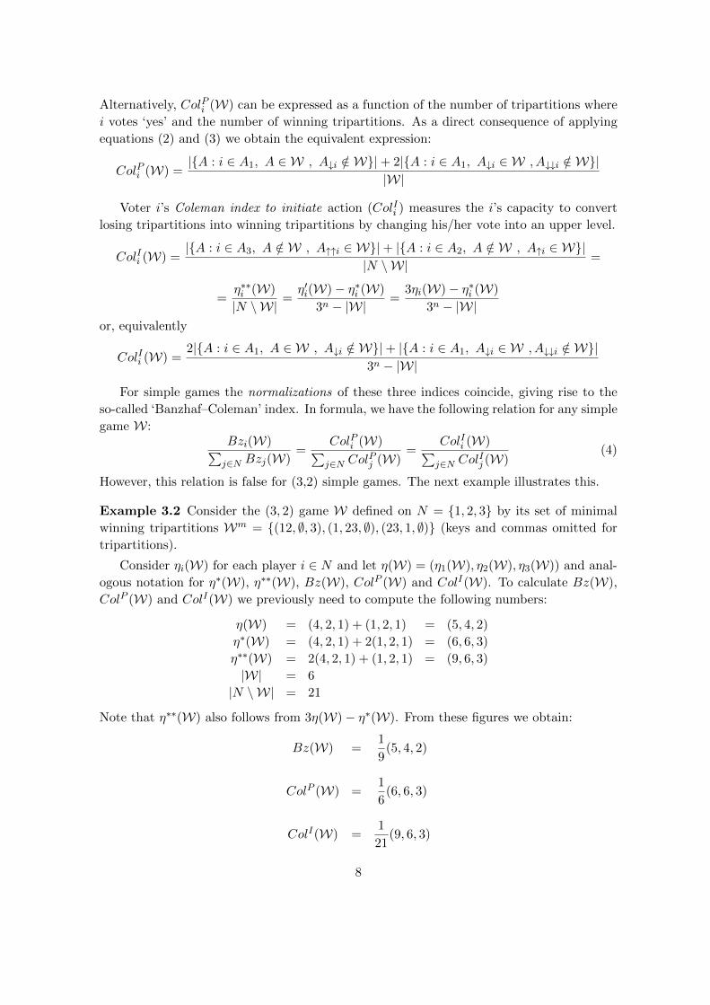
Example 3.2 Consider the (3, 2) game W defined on N = 1, 2, 3 by its set of minimal
winning tripartitions Wm = (12, ∅, 3), (1, 23, ∅), (23, 1, ∅) (keys and commas omitted for
tripartitions).
Consider ηi(W) for each player i ∈ N and let η(W) = (η1(W), η2(W), η3(W)) and anal-
ogous notation for η∗(W), η∗∗(W), Bz(W), ColP (W) and ColI(W). To calculate Bz(W),
ColP (W) and ColI(W) we previously need to compute the following numbers:
η(W) = (4, 2, 1) + (1, 2, 1) = (5, 4, 2)
η∗(W) = (4, 2, 1) + 2(1, 2, 1) = (6, 6, 3)
η∗∗(W) = 2(4, 2, 1) + (1, 2, 1) = (9, 6, 3)
|W| = 6
|N \W| = 21
Note that η∗∗(W) also follows from 3η(W)− η∗(W). From these figures we obtain:
Bz(W) =1
9(5, 4, 2)
ColP (W) =1
6(6, 6, 3)
ColI(W) =1
21(9, 6, 3)
8

The relation for simple games given in (4) is not true for (3,2) games as is illustrated for
W. Indeed,Bz(W)∑
j∈N Bzj(W)=
1
11(5, 4, 2)
ColP (W)∑j∈N ColPj (W)
=1
15(6, 6, 3)
ColI(W)∑j∈N ColIj (W)
=1
18(9, 6, 3)
Concerning the Rae index and I(W) it is not difficult to check that
Rae(W) =1
27(14, 13, 11) while I(W) =
1
27(4, 5, 7)
The lack of proportionality among these three indices for (3,2) games tells us that these are three independent concepts. This difference with simple games is very important. For instance, the proportionality for simple games implies that these three indices are ordinally equivalent (see [4] and [12] for ordinal equivalence of power indices for simple games), whereas for (3,2) games they do not necessarily need to be ordinally equivalent, and hence they can rank voters in different orders.
There exists a linear relationship between the Rae and Banzhaf indices for simple games
which is
Raei(W) =1
2+
1
2Bzi(W) (5)
but the next proposition shows that a different linear relationship holds for (3,2) games:
Proposition 3.3 For each (3,2) game W and i ∈ N it holds
Raei(W) =1
3+
1
3Bzi(W). (6)
Proof: It is enough to prove that |A : i ∈ A1, A ∈ W| + |A : i ∈ A3, A /∈ W| =3n−1 + ηi(W) and dividing by 3n we get the equality. To see this, consider any tripartition
of those counted in ηi(W), i.e. with i being positively crucial, and change (if necessary)
his/her vote to the abstention. Let A one of these tripartitions for which i abstains; as i
is crucial in it his/her vote after the swap will coincide with the output in both A↑i and in
A↓i. Hence, i will be successful in 2ηi(W) tripartitions. Consider now one of the remaining
3n−1 − ηi(W) tripartitions for which i abstains. In such a situation, i will be successful in
only one of the two next: A↑i or A↓i tripartitions, since his/her vote is indifferent to the
final result. In summary, i will be successful in 2 · ηi(W) + (3n−1 − ηi(W)) = 3n−1 + ηi(W).
¤
Relationship (6) for (3,2) games is different from relationship (5) for simple games. We can give an interpretation of Equation (6) for (3,2) games as that Penrose [18] did for
9

equation (5) for simple games. The power of the individual vote can be measured by the
amount by which her chance of being on the winning side exceeds one third. the power, thus
defined, is the same as one third the likelihood of a situation in which an individual vote can
be decisive. Penrose’s measure of power for (3,2) games would correspond to (1/3)Bzi(W).
As 0 ≤ Bzi(W) ≤ 1 for all i ∈ N and (3,2) game W, it trivially follows
1
3≤ Raei(W) ≤ 2
3. (7)
From Equations (1) and (6) also follow:
Ii(W) =1
3− 1
3Bzi(W)
and therefore
0 ≤ Ii(W) ≤ 1
3(8)
for all i ∈ N and (3,2) game W. In contrast to Equations (7) and (8) for simple games the
bounds are:1
2≤ Raei(W) ≤ 1 and 0 ≤ Ii(W) ≤ 1
2.
K¨onig and Br¨auninger’s (3,2) extension The extension of the K¨onig and Br¨auninger voter i’s inclusiveness for simple games [15] to (3,2) games is direct if we take into account that its meaning is to measure the success proportion of a player with respect to the collective success:
KBi(W) =number of winning tripartitions with i voting ‘yes’
total number of winning tripartitions
or, equivalently
KBi(W) =|A : i ∈ A1, A ∈ W|
|W|Note that if voter i ∈ N has yes–veto, i.e. A ∈ W implies i ∈ A1 then KBi(W) = 1.
If voter i ∈ N is null, i.e. A ∈ Wm implies i ∈ A3 then KBi(W) = 1/2. However,
KBi(W) = 1/2 is not exclusive for null voters in (3,2) games. Thus,
1
2≤ KBi(W) ≤ 1
for every (3,2) game and each i ∈ N . These bounds are the same for simple games, but
there KBi(W) = 1/2 iff i is null in the simple game W.
Following Coleman’s idea one may consider (even for simple games) an alternative in-
dex J(W) that measures the (negative) success proportion of a player with respect to the
collective failure:
Ji(W) =number of losing tripartitions with i voting ‘no’
total number of losing tripartitions
or, equivalently
Ji(W) =|A : i ∈ A3, A /∈ W|
|N \W|
10

The two indices above can be regarded as measures of success, now we can define anal-
ogous notions for unsuccess. Let
Li(W) =number of winning tripartitions with i voting ‘no’
total number of winning tripartitions
and
Mi(W) =number of losing tripartitions with i voting ‘yes’
total number of losing tripartitions
Consider now Example 3.2. It is not difficult to check that:
KB(W) =1
6(5, 4, 3)
J(W) =1
21(9, 9, 8)
L(W) =1
6(1, 2, 3)
M(W) =1
21(5, 4, 3)
4 Success, unsuccess and decisiveness in (3, 2) games
In this section we extend the approach followed by Laruelle and Valenciano in [17] for simple
games to (3,2) games.
4.1 Ex post model
First let’s consider the situation ex post, that is, once a committee voted on a given proposal, a tripartition has emerged, and this tripartition has prescribed the final outcome, i.e. passage or rejection of the proposal. A distinction can be made between voters. If the proposal is accepted (rejected), those voters who voted in favour (against) are satisfied with the result, while the others are not. Extending Barry’s contribution for simple games [1], we will say that they have been successful. Thus, being successful means obtaining the outcome—acceptance or rejection— that one voted for. We also say that a successful voter has been decisive in a vote if his/her vote was crucial: i.e., if he/she had changed his/her vote the outcome would have been different. Note that the ex post notions below are binary definitions for each player.
Success ex post (3,2) extension
Definition 4.1 After a decision is made according to a (3,2) game W, if the resulting
configuration of votes is tripartition A,
11

(i) Voter i is said to have been successful if the decision coincides with voter i’s vote, i.e.
iff
(i ∈ A1, A ∈ W) or (i ∈ A3, A /∈ W)
(ii) Voter i is said to have been unsuccessful if the decision is contrary with voter i’s vote,
i.e. iff
(i ∈ A1, A /∈ W) or (i ∈ A3, A ∈ W)
(iii) Voter i is said to have been neutral if voter i abstains, i.e. iff
i ∈ A2
Note that for simple games there are not neutral voters.
Decisiveness ex post (3,2) extension
Definition 4.2 After a decision is made according to a (3,2) game W, if the resulting
configuration of votes is tripartition A,
(i) Voter i is said to have been successfully decisive, if he/she was successful and his/her
vote was critical to that success, i.e. iff
(i ∈ A1, A ∈ W, A↓↓i /∈ W) or (i ∈ A3, A /∈ W, A↑↑i ∈ W)
(ii) Voter i is said to have been neutrally decisive, if he/she was neutral and his/her vote
was critical to the outcome, i.e. iff
(i ∈ A2, A ∈ W, A↓i /∈ W) or (i ∈ A2, A /∈ W, A↑i ∈ W)
Neutrally decisiveness is a new concept with respect to the ex post model for simple
games.
Luckiness ex post (3,2) extension
Definition 4.3 After a decision is made according to a (3,2) game W, if the resulting
configuration of votes is tripartition A,
(i) Voter i is said to have been lucky, i.e. iff
(i ∈ A1, A ∈ W, A↓↓i ∈ W) or (i ∈ A3, A /∈ W, A↑↑i /∈ W)
(ii) Voter i is said to have been neutrally indecisive, if he/she was neutral and his/her
vote was not critical to the outcome, i.e. iff
(i ∈ A2, A ∈ W, A↓i ∈ W) or (i ∈ A2, A /∈ W, A↑i /∈ W)
12
Neutrally indecisiveness is also a new concept with respect to the ex post model for
simple games.
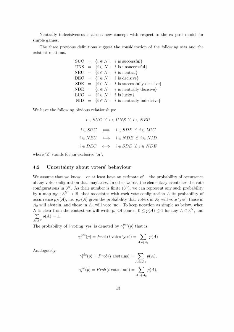
The three previous definitions suggest the consideration of the following sets and the
existent relations.
SUC = i ∈ N : i is successfulUNS = i ∈ N : i is unsuccessfulNEU = i ∈ N : i is neutralDEC = i ∈ N : i is decisiveSDE = i ∈ N : i is successfully decisiveNDE = i ∈ N : i is neutrally decisiveLUC = i ∈ N : i is luckyNID = i ∈ N : i is neutrally indecisive
We have the following obvious relationships:
i ∈ SUC Y i ∈ UNS Y i ∈ NEU
i ∈ SUC ⇐⇒ i ∈ SDE Y i ∈ LUC
i ∈ NEU ⇐⇒ i ∈ NDE Y i ∈ NID
i ∈ DEC ⇐⇒ i ∈ SDE Y i ∈ NDE
where ‘Y’ stands for an exclusive ‘or’.
4.2 Uncertainty about voters’ behaviour
We assume that we know —or at least have an estimate of— the probability of occurrence
of any vote configuration that may arise. In other words, the elementary events are the vote
configurations in 3N . As their number is finite (3n), we can represent any such probability
by a map pN : 3N → R, that associates with each vote configuration A its probability of
occurrence pN (A), i.e. pN (A) gives the probability that voters in A1 will vote ‘yes’, those in
A2 will abstain, and those in A3 will vote ‘no’. To keep notation as simple as below, when
N is clear from the context we will write p. Of course, 0 ≤ p(A) ≤ 1 for any A ∈ 3N , and∑A∈3N
p(A) = 1.
The probability of i voting ‘yes’ is denoted by γyesi (p) that is
γyesi (p) = Prob (i votes ‘yes’) =∑
A:i∈A1
p(A)
Analogously,
γabsi (p) = Prob (i abstains) =∑
A:i∈A2
p(A),
γnoi (p) = Prob (i votes ‘no’) =∑
A:i∈A3
p(A),
13
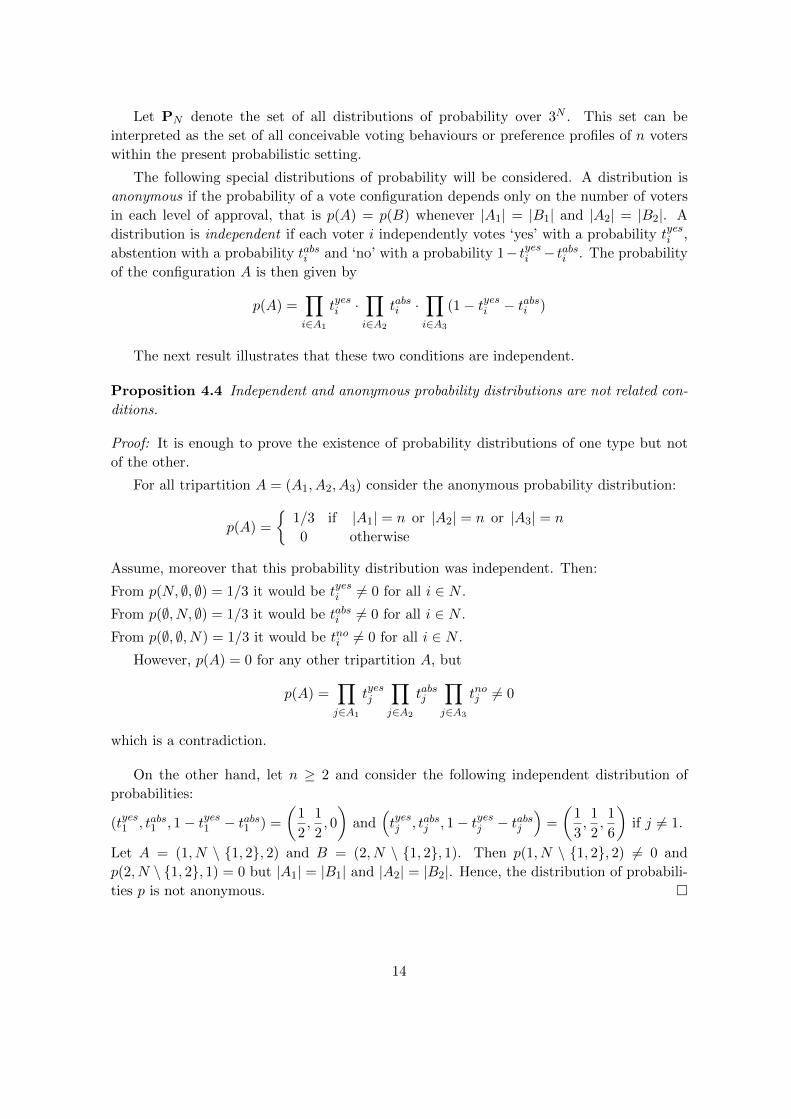
Let PN denote the set of all distributions of probability over 3N . This set can be
interpreted as the set of all conceivable voting behaviours or preference profiles of n voters
within the present probabilistic setting.
The following special distributions of probability will be considered. A distribution is
anonymous if the probability of a vote configuration depends only on the number of voters
in each level of approval, that is p(A) = p(B) whenever |A1| = |B1| and |A2| = |B2|. A
distribution is independent if each voter i independently votes ‘yes’ with a probability tyesi ,
abstention with a probability tabsi and ‘no’ with a probability 1− tyesi − tabsi . The probability
of the configuration A is then given by
p(A) =∏
i∈A1
tyesi ·∏
i∈A2
tabsi ·∏
i∈A3
(1− tyesi − tabsi )
The next result illustrates that these two conditions are independent.
Proposition 4.4 Independent and anonymous probability distributions are not related con-
ditions.
Proof: It is enough to prove the existence of probability distributions of one type but not
of the other.
For all tripartition A = (A1, A2, A3) consider the anonymous probability distribution:
p(A) =
1/3 if |A1| = n or |A2| = n or |A3| = n
0 otherwise
Assume, moreover that this probability distribution was independent. Then:
From p(N, ∅, ∅) = 1/3 it would be tyesi 6= 0 for all i ∈ N .
From p(∅, N, ∅) = 1/3 it would be tabsi 6= 0 for all i ∈ N .
From p(∅, ∅, N) = 1/3 it would be tnoi 6= 0 for all i ∈ N .
However, p(A) = 0 for any other tripartition A, but
p(A) =∏
j∈A1
tyesj
∏
j∈A2
tabsj
∏
j∈A3
tnoj 6= 0
which is a contradiction.
On the other hand, let n ≥ 2 and consider the following independent distribution of
probabilities:
(tyes1 , tabs1 , 1− tyes1 − tabs1 ) =
(1
2,1
2, 0
)and
(tyesj , tabsj , 1− tyesj − tabsj
)=
(1
3,1
2,1
6
)if j 6= 1.
Let A = (1, N \ 1, 2, 2) and B = (2, N \ 1, 2, 1). Then p(1, N \ 1, 2, 2) 6= 0 and
p(2, N \ 1, 2, 1) = 0 but |A1| = |B1| and |A2| = |B2|. Hence, the distribution of probabili-
ties p is not anonymous. ¤
14

Proposition 4.5 If a distribution is both anonymous and independent then each voter votes
‘yes’ with a probability tyes, abstains with probability tabs and votes no with probability 1 −tyes − tabs, and the probability of the configuration A is then given by
p(A) = (tyes)a1(tabs)a2(1− tyes − tabs)n−a1−a2
Proof: Let n ≥ 2 Consider the following three pairs of tripartitions for any pair of voters
i, j ∈ N :
(i, j,N \ i, j), (j, i,N \ i, j),(i,N \ i, j, j), (j,N \ i, j, i),(N \ i, j, i, j), (N \ i, j, j, i).
From anonymity and independence these three pairs lead to the respective equations:
tyesi
tyesj
=tabsi
tabsj
,tyesi
tyesj
=tnoitnoj
,tabsi
tabsj
=tnoitnoj
Lettyesi
tyesj
=tabsi
tabsj
=tnoitnoj
= M
If M 6= 1, then either tyesi + tabsi + tnoi 6= 1 or tyesj + tabsj + tnoj 6= 1 which would be a contradic-
tion. Hence,M = 1 and tyesi = tyesj , tabsi = tabsj and tnoi = tnoj for each pair of voters i and j. ¤
An anonymous and independent distribution is, in fact, a probability distribution, i.e.
n∑
a1=0
n−a1∑
a2=0
(n
a1
)(n− a1a2
)(tyes)a1 · (tabs)a2 · (1− tyes − tabs)n−a1−a2 = 1
because the expression of the left hand–side can be written as
[tyes + tabs + (1− tyes − tabs)]n
Three special cases of anonymous and independent distributions that accumulate some
symmetry deserve to be mentioned.
1. When all vote configuration have the same probability, denoted by
p∗(A) =1
3n
for all tripartition A. This is equivalent to assuming that each voter, independently of
the others, votes ‘yes’ with probability 1/3, abstains with probability 1/3, and votes
‘no’ with probability 1/3. Thus this probability accumulates all symmetries: it is
anonymous and independent, with equal inclination towards ‘yes’, ‘abstention’ and
‘no’.
15

2. Another significant vote configuration is when all voters are active, without abstainers,
and with equal inclination towards ‘yes’ and ‘no’. This is equivalent to assuming that
each voter, independently of the others, votes ‘yes’ with probability 1/2, abstains with
probability 0 and votes ‘no’ with probability 1/2.
p∗∗(A) =
12n , if a2 = 0;
0, if a2 > 0.
for all configurations A ∈ 3N and |A2| = a2.
3. As Felsenthal and Machover [8] suggest, a more cautious approach would be to take the
probability 1− 2p of abstention as an undetermined parameter in the general theory,
leaving 2p to be shared equally between ‘no’ and ‘yes’. In any application of the theory,
the value 1 − 2p might be determined on the basis of specific arguments, including
perhaps empirical data. This would lead us to the family of vote configurations with
equal inclination towards ‘yes’, and ‘no’, which is an extension of vote configuration
p∗. It presupposes the knowledge of the independent probability that a player will
actively participate in the election. Assume that this probability to actively vote is 2p
with p < 1/2 and it is equally distributed between ‘yes’ and ‘no’. This is equivalent
to assuming that each voter, independently of the others, votes ‘yes’ with probability
p, abstains with probability 1− 2p, and votes ‘no’ with probability p.
p∗∗∗(A) = pn−a2(1− 2p)a2 if p < 1/2
for all configurations A ∈ 3N and |A2| = a2. Braham and Steffen [2] argue that
abstention is a totally different action and voters first decide whether they want to
form an opinion on the issue and if the answer is yes, then they vote. This would
suggest a fourth probability distribution with the actively vote 2p distributed between
‘yes’ and ‘no’ in a non–necessarily symmetric way.
4.3 Ex ante model
Assume that a probability distribution over vote configurations p enters the picture as a
second input besides W that governs decisions in a (3,2) game. In a voting situation thus
described by pair (W, p) the ease of passing proposals or probability of acceptance is given
by
α(W, p) = Prob (acceptance) =∑
A:A∈Wp(A)
Furthermore, success, decisiveness and luckiness can also be defined ex ante. It suffices to
replace the sure configuration A by the random vote configuration specified by p in ex post
Definitions 4.1, 4.2, 4.3. This yields the following extension of these concepts.
Success ex ante (3,2) extension
16

Definition 4.6 Let (W, p) be an N voting situation, where W is the (3,2) game and p ∈ PN
is the probability distribution over vote configurations, and let i ∈ N :
(i) Voter i’s (ex ante) success is the probability that i is successful:
ΩSUCi (W, p) = Prob (i is successful) =
∑
A:i∈A1A∈W
p(A) +∑
A:i∈A3A/∈W
p(A)
(ii) Voter i’s (ex ante) failure is the probability that i is unsuccessful
ΩUNSi (W, p) = Prob (i is unsuccessful) =
∑
A:i∈A1A/∈W
p(A) +∑
A:i∈A3A∈W
p(A)
(iii) Voter i’s (ex ante) neutrality is the probability that i is neutral
ΩNEUi (W, p) = Prob (i is neutral) =
∑
A:i∈A2
p(A)
Decisiveness ex ante (3,2) extension
Definition 4.7 Let (W, p) be an N voting situation, where W is the (3,2) simple game and
p ∈ PN is the probability distribution over vote configurations, and let i ∈ N :
(i) Voter i’s (ex ante) success decisiveness is the probability that i is successfully decisive:
ΦSDEi (W, p) = Prob (i is successfully decisive) =
∑
A : i ∈ A1
A ∈ WA↓↓i /∈ W
p(A) +∑
A : i ∈ A3
A /∈ WA↑↑i ∈ W
p(A) (9)
=
a︷ ︸︸ ︷∑
A:i∈A1
A∈WA↓i /∈W
p(A)+
b︷ ︸︸ ︷∑
A:i∈A1
A↓i∈WA↓↓i /∈W
p(A)
+
c︷ ︸︸ ︷∑
A:i∈A3
A/∈WA↑i∈W
p(A)+
d︷ ︸︸ ︷∑
A:i∈A3
A↑i /∈WA↑↑i∈W
p(A)
(ii) Voter i’s (ex ante) neutral decisiveness, is the probability that i is neutrally decisive
ΦNDEi (W, p) = Prob(i is neutrally decisive) =
e︷ ︸︸ ︷∑
A : i ∈ A2
A ∈ WA↓i /∈ W
p(A)+
f︷ ︸︸ ︷∑
A : i ∈ A2
A /∈ WA↑i ∈ W
p(A) (10)
(iii) Voter i’s (ex ante) decisiveness, is the probability that i is successfully decisive and
neutrally decisive, i.e.
ΦDECi (W, p) = ΦSDE
i (W, p) + ΦNDEi (W, p) (11)
17

Obviously ΦSDEi (W, p) ≤ ΦDEC
i (W, p).
Note that the parameters a, b, c, d, e and f that respectively appear in (9) and (10) are
defined for each voter and are functions of W and p, however in some places we will simply
write a instead of the more precise expression ai(W, p) and the same holds for the other five
parameters considered: b, c, d, e and f .
Note that strictly speaking i’s decisiveness depends only on the other voter’s behaviour,
not on his/her own. To see this, voter i’s decisiveness can be rewritten as
ΦDECi (W, p) =
∑
A:i∈A1
A∈WA↓i /∈W
[p(A) + p(A↓i) + p(A↓↓i)] +∑
A:i∈A1
A↓i∈WA↓↓i /∈W
[p(A) + p(A↓i) + p(A↓↓i)]
Such decomposition is held after reordering the six addends of ΦDECi : first (a), (f) and (d),
second (b), (c) and (e). Observe that for each A, [p(A)+p(A↓i)+p(A↓↓i)] is the probabilityof all voters in A1 \ i voting ‘yes’, those in A2 abstain and those in N \ (A1 ∪A2) voting
‘no’. In this case, whatever voter i’s vote, he/she is decisive, while the measures of success
depend on all voters’ behaviour.
Luckiness ex ante (3,2) extension
Definition 4.8 Let (W, p) be an N voting situation, where W is the (3,2) game and p ∈ PN
is the probability distribution over vote configurations, and let i ∈ N :
(i) Voter i’s (ex ante) luckiness is the probability that i is successfully lucky:
ΛLUCi (W, p) = Prob (i is lucky) =
∑
A : i ∈ A1
A↓↓i ∈ W
p(A) +∑
A : i ∈ A3
A↑↑i /∈ W
p(A)
(ii) Voter i’s (ex ante) neutrally indecisiveness or the probability that i is ‘neutrally inde-
cisive’
ΛNINDi (W, p) =
∑
A : i ∈ A2
A↓i ∈ W
p(A) +∑
A : i ∈ A2
A↑i /∈ W
p(A)
Barry’s equation and some other equations From the three previous definitions it
trivially follows the next two equations. The first equation concerns the ex ante voter i’s
satisfaction, while the second equation concerns decisiveness.
ΩSUCi (W, p) + ΩUNS
i (W, p) + ΩNEUi (W, p) = 1
ΦDECi (W, p) = ΦSDE
i (W, p) + ΦNDEi (W, p)
The Barry’s equation for simple games for all probability distribution p on 2N :
Ωi(W, p) = Φi(W, p) + Λi(W, p)
18
is still true for (3,2) simple games but it can be decomposed into two separate identities.
The first identity is the direct extension of Barry’s (success) equation for simple games,
while the second is a new version for neutrality.
ΩSUCi (W, p) = ΦSDE
i (W, p) + ΛLUCi (W, p)
ΩNEUi (W, p) = ΦNDE
i (W, p) + ΛNINDi (W, p)
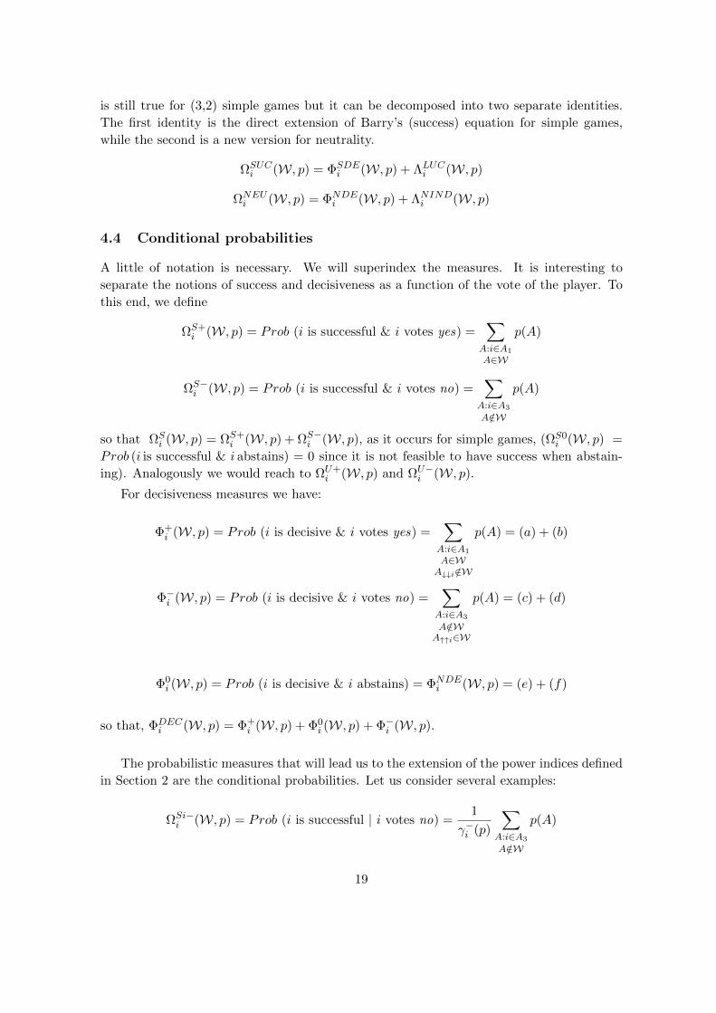
4.4 Conditional probabilities
A little of notation is necessary. We will superindex the measures. It is interesting to
separate the notions of success and decisiveness as a function of the vote of the player. To
this end, we define
ΩS+i (W, p) = Prob (i is successful & i votes yes) =
∑
A:i∈A1
A∈W
p(A)
ΩS−i (W, p) = Prob (i is successful & i votes no) =
∑
A:i∈A3
A/∈W
p(A)
so that ΩSi (W, p) = ΩS+
i (W, p) + ΩS−i (W, p), as it occurs for simple games, (ΩS0
i (W, p) =
Prob (i is successful & i abstains) = 0 since it is not feasible to have success when abstain-
ing). Analogously we would reach to ΩU+i (W, p) and ΩU−
i (W, p).
For decisiveness measures we have:
Φ+i (W, p) = Prob (i is decisive & i votes yes) =
∑
A:i∈A1
A∈WA↓↓i /∈W
p(A) = (a) + (b)
Φ−i (W, p) = Prob (i is decisive & i votes no) =
∑
A:i∈A3
A/∈WA↑↑i∈W
p(A) = (c) + (d)
Φ0i (W, p) = Prob (i is decisive & i abstains) = ΦNDE
i (W, p) = (e) + (f)
so that, ΦDECi (W, p) = Φ+
i (W, p) + Φ0i (W, p) + Φ−
i (W, p).
The probabilistic measures that will lead us to the extension of the power indices defined
in Section 2 are the conditional probabilities. Let us consider several examples:
ΩSi−i (W, p) = Prob (i is successful | i votes no) = 1
γ−i (p)
∑
A:i∈A3
A/∈W
p(A)
19
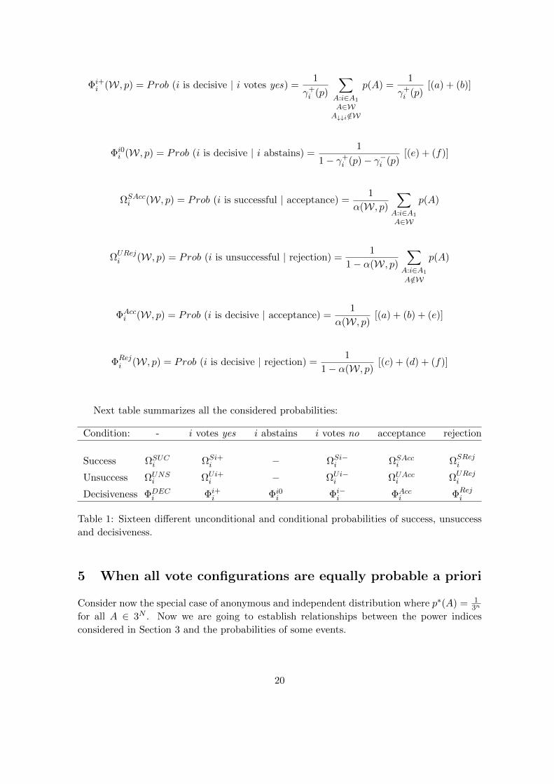
Φi+i (W, p) = Prob (i is decisive | i votes yes) = 1
γ+i (p)
∑
A:i∈A1
A∈WA↓↓i /∈W
p(A) =1
γ+i (p)[(a) + (b)]
Φi0i (W, p) = Prob (i is decisive | i abstains) = 1
1− γ+i (p)− γ−i (p)[(e) + (f)]
ΩSAcci (W, p) = Prob (i is successful | acceptance) = 1
α(W, p)
∑
A:i∈A1
A∈W
p(A)
ΩUReji (W, p) = Prob (i is unsuccessful | rejection) = 1
1− α(W, p)
∑
A:i∈A1
A/∈W
p(A)
ΦAcci (W, p) = Prob (i is decisive | acceptance) = 1
α(W, p)[(a) + (b) + (e)]
ΦReji (W, p) = Prob (i is decisive | rejection) = 1
1− α(W, p)[(c) + (d) + (f)]
Next table summarizes all the considered probabilities:
Condition: - i votes yes i abstains i votes no acceptance rejection
Success ΩSUCi ΩSi+
i − ΩSi−i ΩSAcc
i ΩSReji
Unsuccess ΩUNSi ΩUi+
i − ΩUi−i ΩUAcc
i ΩUReji
Decisiveness ΦDECi Φi+
i Φi0i Φi−
i ΦAcci ΦRej
i
Table 1: Sixteen different unconditional and conditional probabilities of success, unsuccess
and decisiveness.
5 When all vote configurations are equally probable a priori
Consider now the special case of anonymous and independent distribution where p∗(A) = 13n
for all A ∈ 3N . Now we are going to establish relationships between the power indices
considered in Section 3 and the probabilities of some events.
20

Success and Rae (3,2) measures
Raei(W) =|A : i ∈ A1, A ∈ W|
3n+
|A : i ∈ A3, A /∈ W|3n
= ΩSUCi (W, p∗).
Decisiveness, Banzhaf and Coleman (3,2) measures To link the Banzhaf measure
for (3,2) games with decisiveness in the context (W, p∗) we need to relate ηi(W) with the
considered decisiveness measures:
Bzi(W) =1
1/3· ηi(W)
3n=
1
γ+i (p∗)
∑
A:i∈A1
A∈WA↓↓i /∈W
p∗(A) = Φi+i (W, p∗)
it holds: Φi+i (W, p∗) = Φi−
i (W, p∗) = Φi0i (W, p∗) = ΦDEC
i (W, p∗); therefore, Bzi(W) is
equivalent to four probabilistic decisiveness measures. This is because γ+i (p∗) = γ−i (p
∗) =γ0i (p
∗) = 1/3, and that (a) + (b) = (c) + (d) = (e) + (f) when p = p∗, since the number of
tripartitions that take part in each pair of addends is the same. Those addends that appear
in (a), (d) and (f) are identical, in which we pass from ones to others by switching voter i
by its different voting options (the same for (b), (c) and (e)). As immediate corollaries, we
have that ΦSDEi (W, p∗) = 2 · ΦNDE
i (W, p∗) and
Bzi(W) = 3[a(W, p∗) + b(W, p∗)]
As Coleman index to prevent action (ColPi ) is equal toη∗i (W)|W| , it is sufficient to relate
η∗i (W) with probability measures to get a probabilistic interpretations for ColPi . Analo-
gously, as Coleman index to initiate action (ColIi ) is equal toη∗i (W)|W| , it is sufficient to relate
η∗∗i (W) with probability measures to get a probabilistic interpretations for ColIi .
As |W| = α(W, p∗), η∗i (W) = [(a) + (b) + (e)] and η∗∗i (W) = [(c) + (d) + (f)] it follows:
ColPi (W) =1
α(W, p∗)[(a) + (b) + (e)] = ΦAcc
i (W, p∗)
ColIi (W) =1
1− α(W, p∗)[(c) + (d) + (f)] = ΦRej
i (W, p∗)
Alternative expressions of Coleman’s measures are:
ColPi (W) =a(W, p∗) + 2b(W, p∗)
A(W)
ColIi (W) =2a(W, p∗) + b(W, p∗)
1−A(W)
21

Konig and Brauninger and other probabilistic (3,2) measures The nature of the
inclusiveness index is to measure the rate of success of a player with respect to the collective
success, that is:
KBi(W) =|A : i ∈ A1, A ∈ W|
|W|By using the same argument that in the Coleman’s measures we obtain:
KBi(W) =1
α(W, p∗)|A : i ∈ A1, A ∈ W|
3n= ΩSAcc
i (W, p∗)
For the other three indices J , L and M we have analogous relationships.
Next table summarizes the relations studied in this Section for p = p∗. Note that the
complete family of (3,2) measures introduced in Section 3 appear in the table: Rae, Bz,
ColP , ColI , KB, J , L, M . Thus, all these eight measures have interpretation as probabilities
of some events in the context (W, p∗).
Condition: none i votes yes i abstains i votes no acceptance rejection
Success Raei(W) ΩSi+i − ΩSi−
i KBi(W) Ji(W)
Unsuccess Ii(W) ΩUi+i − ΩUi−
i Li(W) Mi(W)
Decisiveness Bzi(W) Bzi(W) Bzi(W) Bzi(W) ColPi (W) ColIi (W)
Table 2: Relationships between power indices for (3,2) games and the current probabilistic
model.
For simple games Laruelle and Valenciano [16] prove that the relation
Ωi(W, p) =1
2+
1
2Φi(W, p)
holds for all simple game W and probability distribution p on 2N if and only if p = p∗,i.e. under the assumption that all vote configurations are equally probable. Thus, for each
p 6= p∗ there is a simple game W such that
Ωi(W, p) 6= 1
2+
1
2Φi(W, p)
Hence, for simple games success and decisiveness are not only conceptually different but also
analytically independent as there is no general way to derive one concept from the other if
p 6= p∗.
But, what happen for (3,2) games? A natural but slightly different extension of Laruelle
and Valenciano’s result for simple games holds for (3,2) games. Indeed, part (i) of Proposi-
tion 5.1 follows the same guidelines of their proof for simple games, part (ii) is derived by
applying their result for simple games, while part (iii) follows from part (i) and by consid-
ering p 6= p∗ and three (or more voting rules) with the same number of voters giving rise to
an incompatible system with unknowns k1 and k2.
22

Proposition 5.1 For all i ∈ N and real numbers k1 and k2 it yields:
i) ΩSUCi (W, p) =
1
3+
1
3ΦDECi (W, p) for all (3,2) game W if and only if p = p∗.
ii) Ωi(V, p) = 1
2+
1
2Φi(V, p) for all projection V of an arbitrary (3,2) game W if and
only if p = (1/2, 1/2).
iii) ΩSUCi (W, p) = k1 + k2Φ
DECi (W, p) for all (3,2) game W if and only if p = p∗.
Example 5.2 Consider again Example 3.2, i.e. the (3, 2) game W defined on N = 1, 2, 3by its set of minimal winning tripartitions Wm = (12, ∅, 3), (1, 23, ∅), (23, 1, ∅) (keys and
commas omitted for tripartitions).
Consider decisiveness for each player, i.e.
ΦDEC(W, p) = (ΦDEC1 (W, p),ΦDEC
2 (W, p),ΦDEC3 (W, p))
As we have seen in (9), (10) and (11): ΦDECi (W, p) = ai + bi + ci + di + ei + fi. Let
a = (a1, a2, a3) and analogous notation for b, c, d, e and f .
For voting configuration p∗ then one may easily check that: a = d = f and b = c = e
independently of W. Moreover, for the particular W of this example we have:
a = d = f = 133(4, 2, 1) =
(427 ,
227 ,
127
)
b = c = e = 133(1, 2, 1) =
(127 ,
227 ,
127
)
so that:
ΦDEC(W, p∗) = (ΦDEC1 (W, p∗),ΦDEC
2 (W, p∗),ΦDEC3 (W, p∗)) =
(15
27,12
27,6
27
)
while for success we obtain the expected result according to Proposition 5.1-(i)
ΩSUC(W, p∗) =(14
27,13
27,11
27
).
Consider now p∗∗ then one may easily check that:
ΦDEC(W, p∗∗) =(4
8,4
8,0
8
)and ΩSUC(W, p∗∗) =
(6
8,6
8,4
8
)
so that one might suspect that the relationship:
Ωi(W, p∗∗) =1
2+
1
2Φi(W, p∗∗) (12)
is true, but this is not the case as the following example illustrates. Let
Wm = (1, 2, 3), (13, ∅, 2), (2, 13, ∅) then:
ΦDEC(W, p∗∗) =(6
8,2
8,1
8
)and ΩSUC(W, p∗∗) =
(7
8,5
8,5
8
)
Thus, Equation (12) is not true for this (3,2) game.
23

6 Computation of power indices for (3,2) games
In this section, we show how to compute for weighted (3,2) games, in an efficient way, the indices we have been working with along the previous sections. To this end, we extend to weighted (3,2) games the idea by Brams and Affuso [3], which consists of using generating functions to obtain η(W) as the sum of some of its coefficients. We want to note that the procedure below can be easily extended to the class of (j,k) games, considered in Freixas and Zwicker [13], and similar indices to those considered in Section 3 of this paper.
Let’s consider a weighted (3,2) simple game as described in Definition 2.3 with quota q
and weights wY (p) and wN (p) for each player p ∈ N . We build the global generating func-
tion f(x) and the individual generating functions fi(x) in the following way:
f(x) =∏
p∈N(xw
N (p) + 1 + xwY (p)) =
WY∑
j=WN
αjxj
fi(x) =∏
p6=i
(xwN (p) + 1 + xw
Y (p)) =
WY −wY (i)∑
j=WN−wN (i)
αjxj
where W Y =∑
p∈NwY (p), WN =
∑
p∈NwN (p).
Once the individual generating function is computed, we have to sum their relevant
coefficients to get the value of ηi(W). Note that each αj indicates the number of tripartitions
with total weight j that can be set up using any of the N players apart from i, so that the
relevant coefficients are those referred to those tripartitions which change their condition
(from winners to losers) when player i descends one single level of approval:
q−wN (i)−1∑
j=q−wY (i)
αj = (αq−wY (i) + ...+ αq−1) + (αq + ...+ αq−wN (i)−1) =
= |A : A ∈ W, A↓i /∈ W, i ∈ A1|+ |A : A ∈ W, A↓i /∈ W, i ∈ A2| = ηi(W)
Recall that here wY (i) ≥ 0 and wN (i) ≤ 0 by the convention to normalize in the middle
level, but this convention is not compulsory to compute indices with generating functions.
A small modification in the previous formula serves to obtain η∗i (W) and η∗∗i (W):
η∗i (W) = (αq−wY (i) + ...+ αq−1) + 2 · (αq + ...+ αq−wN (i)−1)
η∗∗i (W) = 2 · (αq−wY (i) + ...+ αq−1) + (αq + ...+ αq−wN (i)−1)
as it is obvious using the same reasoning which was applied to the Coleman indices’ nume-
rators in Section 3.
24

Rae, Banzhaf and Coleman indices are immediately obtained from these raw ones. The
numerator of the Konig-Brauninger index can also be computed in an analogous way, now
considering as relevant the following coefficients:
WY −wY (i)∑
j=q−wY (i)
αj = (αq−wY (i) + ...+ αWY −wY (i)) = |A : i ∈ A1, A ∈ W|
Note that the sum starts at the same first coefficient as before but ends at the last one, as
we are considering all the winning tripartitions in which voter i votes ‘yes’. To compute the
Konig and Brauninger index denominator (and Coleman’s decisiveness index, as well), we
need to use the global GF :
|W| =WY∑
j=q
αj = αq + αq+1...+ αWY
The other success and unsuccess notions derived from the Konig and Brauninger index
(J(W), L(W) and M(W)) would be computed in similar ways. Let’s check in the next
example that all these procedures work:
Example 6.1 Consider again the game W described in the Example 3.2, in which Wm =
(12, ∅, 3), (1, 23, ∅), (23, 1, ∅). This (3,2) simple game can also be represented as a weighted
(3,2) simple game by [ 2 ; (2,−1), (1,−2), (1,−1)] (where q = 2 and each player’s ‘yes’ and
‘no’ votes appear in brackets). First of all, let’s compute the individual generating function:
f1(x) = (x−2 + 1 + x)(x−1 + 1 + x) = x−3 + x−2 + 2x−1 + 2 + 2x+ x2
f2(x) = (x−1 + 1 + x2)(x−1 + 1 + x) = x−2 + 2x−1 + 2 + 2x+ x2 + x3
f3(x) = (x−1 + 1 + x2)(x−2 + 1 + x) = x−3 + x−2 + x−1 + 3 + x+ x2 + x3
The next step is obtaining the different raw indices using the procedure explained above:
q − wY (1) = 0 q = 2
q − 1 = 1 q − wN (1)− 1 = 2
→ η1(W) = (α0 + α1) + a2 = 4 + 1 = 5
q − wY (2) = 1 q = 2
q − 1 = 1 q − wN (2)− 1 = 3
→ η2(W) = α1 + (α2 + α3) = 2 + 2 = 4
q − wY (3) = 1 q = 2
q − 1 = 1 q − wN (3)− 1 = 2
→ η3(W) = α1 + α2 = 1 + 1 = 2
Indeed, these values coincide with the ones given in Example 3.2. Now we can easily compute
η∗(W) and η∗∗(W):
η∗(W) = (4 + 2 · 1, 2 + 2 · 2, 1 + 2 · 1) = (6, 6, 3)
η∗∗(W) = (2 · 4 + 1, 2 · 2 + 2, 2 · 1 + 1) = (9, 6, 3)
25
Finally, we deal with the KB index. Its numerators for each player are:
|A : 1 ∈ A1, A ∈ W| = α0 + ... = 2 + 2 + 1 = 5
|A : 2 ∈ A1, A ∈ W| = α1 + ... = 2 + 1 + 1 = 4
|A : 3 ∈ A1, A ∈ W| = α1 + ... = 1 + 1 + 1 = 3
while the denominator is obtained from the global generating function:
f(x) = (x−1+1+x2)(x−2+1+x)(x−1+1+x) = x−4+2x−3+3x−2+5x−1+5+5x+3x2+2x3+x4
|W| = α2 + ... = 3 + 2 + 1 = 6
Again, this method provides the same results which were given in the Example considered.
For large values of n = |N |, these calculations can become really tedious. That is why
some mathe-matical software may help. The indices we are showing in the next example
have been computed by an algorithm ran with Maple.
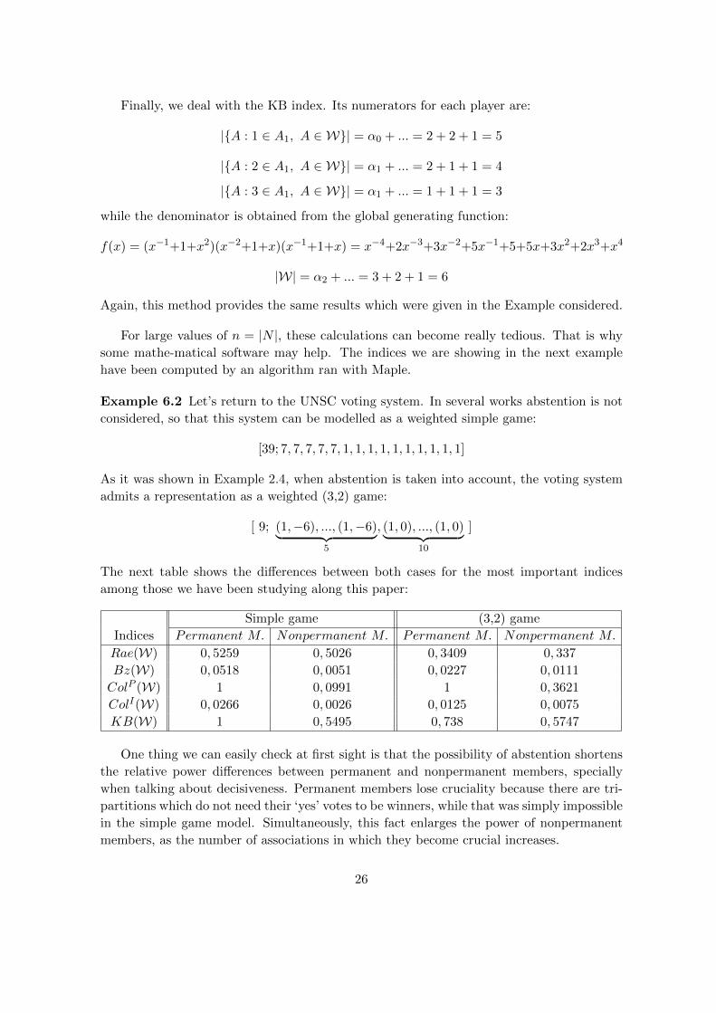
Example 6.2 Let’s return to the UNSC voting system. In several works abstention is not
considered, so that this system can be modelled as a weighted simple game:
[39; 7, 7, 7, 7, 7, 1, 1, 1, 1, 1, 1, 1, 1, 1, 1]
As it was shown in Example 2.4, when abstention is taken into account, the voting system
admits a representation as a weighted (3,2) game:
[ 9; (1,−6), ..., (1,−6)︸ ︷︷ ︸5
, (1, 0), ..., (1, 0)︸ ︷︷ ︸10
]
The next table shows the differences between both cases for the most important indices
among those we have been studying along this paper:
Simple game (3,2) game
Indices Permanent M. Nonpermanent M. Permanent M. Nonpermanent M.
Rae(W) 0, 5259 0, 5026 0, 3409 0, 337
Bz(W) 0, 0518 0, 0051 0, 0227 0, 0111
ColP (W) 1 0, 0991 1 0, 3621
ColI(W) 0, 0266 0, 0026 0, 0125 0, 0075
KB(W) 1 0, 5495 0, 738 0, 5747
One thing we can easily check at first sight is that the possibility of abstention shortens
the relative power differences between permanent and nonpermanent members, specially
when talking about decisiveness. Permanent members lose cruciality because there are tri-
partitions which do not need their ‘yes’ votes to be winners, while that was simply impossible
in the simple game model. Simultaneously, this fact enlarges the power of nonpermanent
members, as the number of associations in which they become crucial increases.
26
Another fact we can observe is the loss of proporcionality between the Banzhaf and
Coleman indices, in the way it was announced in Section 3 (see Example 3.2): while the
proportion of power between permanent and nonpermanent members is exactly the same
(' 10 : 1) for each of the three indices in the simple game model, in the (3,2) game all of
them are considerably different: (Bz ' (2 : 1), (2 : 1) ≤ ColP ≤ (3 : 1), ColI ≤ (2 : 1)).
This is another evidence of the independence of these three concepts when abstention takes
part as an input.
References
[1] B. Barry. Is it better to be powerful or lucky?, part I and part II. Political Studies,28:183–194, 338–352, 1980.
[2] M. Braham and F. Steffen. Voting power in games with abstentions. Power andFairness, 20:333–348, 2003.
[3] S.J. Brams and P.J. Affuso. Power and size: A new paradox. Theory and Decision,
7:29–56, 1976.
[4] F. Carreras and J. Freixas. On ordinal equivalence of power measures given by regularsemivalues. Mathematical Social Sciences, 55:221–234, 2008.
[5] J.S. Coleman. Control of collectivities and the power of a collectivity to act. In
B. Lieberman, editor, Social Choice, pages 269–300. Gordon and Breach, New York,
USA, 1971.
[6] J.S. Coleman. Combinatorics: Individual Interests and Collective Action: selected Es-
says. Cambridge University Press, 1986.
[7] D.S. Felsenthal and M. Machover. Ternary voting games. International Journal of
Game Theory, 26:335–351, 1997.
[8] D.S. Felsenthal and M. Machover. The Measurament of Voting Power: Theory and
practice, problems and paradoxes. Cheltenham: Edward Elgar, 1998.
[9] P.C. Fishburn. The Theory of Social Choice. Princeton: Princeton University Press,1973.
[10] J. Freixas. Banzhaf measures for games with several levels of approval in the input andoutput. Annals of Operations Research, 137:45–66, 2005.
[11] J. Freixas. The Shapley–Shubik power index for games with several levels of approvalin the input and output. Decision Support Systems, 39:185–195, 2005.
[12] J. Freixas. On ordinal equivalence of the Shapley and Banzhaf values. InternationalJournal of Game Theory. DOI: 10.1007/s00182-009-0179-0, 2010.
27

[13] J. Freixas and W.S. Zwicker. Weighted voting, abstention, and multiple levels of ap-
proval. Social Choice and Welfare, 21:399–431, 2003.
[14] J. Freixas and W.S. Zwicker. Anonymous yes–no voting with abstention and multiple
levels of approval. Games and Economic Behavior, 69:428–444, 2009.
[15] T. K¨onig and T. Br¨auninger. The inclusiveness of European decision rules. Journal ofTheoretical Politics, 10:125–142, 1998.
[16] A. Laruelle and F. Valenciano. Semivalues and voting power. International Journal ofGame Theory Review, 5:41–61, 2003.
[17] A. Laruelle and F. Valenciano. Voting and Collective Decision–Making. Cambridge
University Press, 2008.
[18] L.S. Penrose. The elementary statistics of majority voting. Journal of the Royal Sta-tistical Society, 109:53–57, 1946.
[19] R. Pongou, B. Tchantcho, and L. Diffo Lambo. Political influence in multi-choice
institutions : Cyclicity, anonymity and transitivity, forthcoming. Theory and Decision,
2010.
[20] D. Rae. Decision rules and individual values in Constitutional choice. American Polit-ical Sciences Review, 63:40–56, 1969.
[21] A. Rubenstein. Stability of decision systems under majority rule. Journal of Economic
Theory, 23:150–159, 1980.
[22] B. Tchantcho, L. Diffo Lambo, R. Pongou, and B. Mbama Engoulou. Voters’ powerin voting games with abstention: Influence relation and ordinal equivalence of powertheories. Games and Economic Behavior, 64:335–350, 2008.
[23] B. Tchantcho, L. Diffo Lambo, R. Pongou, and J. Moulen. On the equilibrium of votinggames with several levels of approval. Social Choice and Welfare, 34:379–396, 2009.
[24] W.S. Zwicker. Anonymous voting rules with abstention: weighted voting. In S.J. Brams, W.V. Gehrlein, and F.S. Roberts, editors, The Mathematics of Preference, Choice, and Order: Essays in Honor of Peter C. Fishburn, pages 239–258. Heidelberg: Springer,2009.
28