Probabilistic Parameter Uncertainty Analysis of Single ... · Probabilistic Parameter Uncertainty...
93
NASA/TM-2005-213280 Probabilistic Parameter Uncertainty Analysis of Single Input Single Output Control Systems Brett A. Smith Joint Institute for Advancement of Flight Sciences George Washington, University, Hampton, Virginia Sean P. Kenny Langley Research Center, Hampton, Virginia Luis G. Crespo National Institute of Aerospace, Hampton, Virginia March 2005 https://ntrs.nasa.gov/search.jsp?R=20050160469 2020-05-13T01:07:28+00:00Z
Transcript of Probabilistic Parameter Uncertainty Analysis of Single ... · Probabilistic Parameter Uncertainty...

https://ntrs.nasa.gov/search.jsp?R=20050160469 2020-05-13T01:07:28+00:00Z
NASA/TM-2005-213280
Probabilistic Parameter Uncertainty Analysis of Single Input Single Output Control SystemsBrett A. SmithJoint Institute for Advancement of Flight SciencesGeorge Washington, University, Hampton, Virginia
Sean P. KennyLangley Research Center, Hampton, Virginia
Luis G. CrespoNational Institute of Aerospace, Hampton, Virginia
March 2005

The NASA STI Program Office . . . in Profile
Since its founding, NASA has been dedicated to the advancement of aeronautics and space science. The NASA Scientific and Technical Information (STI) Program Office plays a key part in helping NASA maintain this important role.
The NASA STI Program Office is operated by Langley Research Center, the lead center for NASA’s scientific and technical information. The NASA STI Program Office provides access to the NASA STI Database, the largest collection of aeronautical and space science STI in the world. The Program Office is also NASA’s institutional mechanism for disseminating the results of its research and development activities. These results are published by NASA in the NASA STI Report Series, which includes the following report types:
• TECHNICAL PUBLICATION. Reports of completed research or a major significant phase of research that present the results of NASA programs and include extensive data or theoretical analysis. Includes compilations of significant scientific and technical data and information deemed to be of continuing reference value. NASA counterpart of peer-reviewed formal professional papers, but having less stringent limitations on manuscript length and extent of graphic presentations.
• TECHNICAL MEMORANDUM. Scientific and technical findings that are preliminary or of specialized interest, e.g., quick release reports, working papers, and bibliographies that contain minimal annotation. Does not contain extensive analysis.
• CONTRACTOR REPORT. Scientific and technical findings by NASA-sponsored contractors and grantees.
• CONFERENCE PUBLICATION. Collected papers from scientific and technical conferences, symposia, seminars, or other meetings sponsored or co-sponsored by NASA.
• SPECIAL PUBLICATION. Scientific, technical, or historical information from NASA programs, projects, and missions, often concerned with subjects having substantial public interest.
• TECHNICAL TRANSLATION. English-language translations of foreign scientific and technical material pertinent to NASA’s mission.
Specialized services that complement the STI Program Office’s diverse offerings include creating custom thesauri, building customized databases, organizing and publishing research results . . . even providing videos.
For more information about the NASA STI Program Office, see the following:
• Access the NASA STI Program Home Page at http://www.sti.nasa.gov
• Email your question via the Internet to [email protected]
• Fax your question to the NASA STI Help Desk at (301) 621-0134
• Telephone the NASA STI Help Desk at (301) 621-0390
• Write to:NASA STI Help DeskNASA Center for AeroSpace Information7121 Standard DriveHanover, MD 21076-1320

NASA/TM-2005-213280
Probabilistic Parameter Uncertainty Analysis of Single Input Single Output Control SystemsBrett A. SmithJoint Institute for Advancement of Flight SciencesGeorge Washington, University, Hampton, Virginia
Sean P. KennyLangley Research Center, Hampton, Virginia
Luis G. CrespoNational Institute of Aerospace, Hampton, Virginia
National Aeronautics andSpace Administration
Langley Research CenterHampton, Virginia 23681-2199
March 2005

Available from:
NASA Center for AeroSpace Information (CASI) National Technical Information Service (NTIS)7121 Standard Drive 5285 Port Royal RoadHanover, MD 21076-1320 Springfield, VA 22161-2171(301) 621-0390 (703) 605-6000
The use of trademarks or names of manufacturers in this report is for accurate reporting and does not constitute anofficial endorsement, either expressed or implied, of such products or manufacturers by the National Aeronautics andSpace Administration.

iii
Abstract
The current standards for handling uncertainty in control systems use interval bounds for
definition of the uncertain parameters. This type of approach gives no information about the
likelihood of system performance but simply gives the response bounds. When used in design,
current methods of µ-analysis and can lead to overly conservative controller designs. With
these methods worst case conditions are weighted equally with the most likely conditions. This
research explores a unique approach for probabilistic analysis of control systems. Current
reliability methods are examined, First Order Reliability Methods and Monte Carlo using
sampling procedures such as Hammersley Sequence Sampling, showing the strong areas of
each in handling probability. A hybrid method is developed using these reliability tools for
efficiently propagating probabilistic uncertainty through classical control analyses problems.
The method developed is applied to classical Bode and Step response analysis as well as
analysis methods that explore the effects of the uncertain parameters on stability and
performance metrics. The benefits of using this hybrid approach for calculating the mean and
variance of response cumulative distribution functions are shown. Results of the probabilistic
analysis of a missile pitch control system show the added information provided by this hybrid
analysis. Finally, a probability of stability analysis is performed on both the missile pitch
control problem and a benchmark non collocated mass spring system.
H∞
ContentsAbstract .................................................................................................................................... iii
Contents ................................................................................................................................... iv
List of Figures ......................................................................................................................... vii
Nomenclature .......................................................................................................................... ix
Acronyms ...................................................................................................................................x
Chapter 1: Introduction ...........................................................................................................1
Probabilistic Uncertainty ....................................................................................................1
Current State of Probabilistic Control Analysis .................................................................3
Controls ...............................................................................................................................4
Probabilistic and Reliability Analysis .................................................................................6
Sampling and Monte Carlo .................................................................................................7
Reliability Methods ..........................................................................................................10
Probabilistic Analysis of SISO systems ............................................................................11
Classical Response Analysis ............................................................................................11
Parameter Space Analysis ................................................................................................14
Chapter 2: Reliability Methods .............................................................................................16
Sampling and Monte Carlo ...............................................................................................16
Stratified Sampling Methods (Latin Hypercube) .............................................................17
Low Discrepancy Methods and Hammersley Sequence Sampling ..................................19
Justification For Using HSS .............................................................................................21
First Order Reliability Methods (FORM) .........................................................................23
Transformation to Standard Normal Space ......................................................................24
iv

Most Probable Point Determination .................................................................................26
Limit State Approximation and Probability of Failure Calculation .................................26
Chapter 3: Hybrid Approach ................................................................................................28
General Hybrid Method ....................................................................................................28
Tail Refinement Process ...................................................................................................29
Capturing Abnormal Occurrences ....................................................................................33
Hybrid Data Processing and Representation ....................................................................34
Response Analysis Issues .................................................................................................38
Extending to Parameter Space Analysis ...........................................................................40
Performance Metric Analysis ...........................................................................................41
Probability of Instability Analysis ....................................................................................42
Chapter 4: Analysis of Hybrid Method ................................................................................47
Definition of Example Problem #1 ...................................................................................47
Probabilistic Response Plots .............................................................................................49
Bode Analysis ...................................................................................................................49
Step Response Analysis ....................................................................................................51
Comparing the Hybrid Method with Standard Uncertainty Analysis ..............................52
Mean and Variance Benefits of Hybrid Approach ...........................................................54
System Response Code Testing ........................................................................................56
Scalable Testing Techniques ............................................................................................57
Computational Effort Analysis .........................................................................................58
Definition of Example Problem #2 ...................................................................................60
Parameter Space Analysis .................................................................................................62
v

Performance Metric Analysis ...........................................................................................62
Probability of Instability ...................................................................................................66
Chapter 5: Conclusions ..........................................................................................................74
Chapter 6: Future Work ........................................................................................................76
References ................................................................................................................................78
vi

List of Figures
Figure 1-1: Norm bounded Uncertainty vs. Probabilistic Uncertainty........................ 2
Figure 1-2: Parameter Uncertainty Propagation .......................................................... 3
Figure 1-3: Uncertainty Separated Into Delta Block ................................................... 5
Figure 1-4: Probabilistic Bode Response .................................................................. 13
Figure 2-1: Stratified Sampling ................................................................................. 18
Figure 2-2: Monte Carlo Sampling Methods (100 points) A) Random Sample
generation, B) Latin Hypercube Samples, C) Hammersley Sequence
Samples. .............................................................................................. 20
Figure 2-3: Comparison of Sampling Methods for a Standard Normal Distribution 22
Figure 2-4: Nonlinear Transformation from x-space to u-space ............................... 25
Figure 2-5: Schematic of Limit State Approximation ............................................... 27
Figure 3-1: FORM Step Prediction............................................................................ 32
Figure 3-2: Pchip vs. Spline Curve Fitting ................................................................ 37
Figure 3-3: First Order Approximation Problem....................................................... 39
Figure 3-4: Hypercube Scaling Methods ................................................................... 43
Figure 4-1: Classical Pitch Autopilot ........................................................................ 48
Figure 4-2: Probabilistic Bode Analysis.................................................................... 50
Figure 4-3: Probabilistic Step Response.................................................................... 52
Figure 4-4: Hybrid Method Compared to D Block Representation of Uncertainty .. 53
Figure 4-5: Mean Computation Error for Hybrid and HSS Methods ........................ 55
Figure 4-6: Variance Computation Error for Hybrid and HSS Methods................... 56
Figure 4-7: Bode Magnitude Computational Time Analysis .................................... 58
vii
Figure 4-8: Bode Phase Computational Effort Analysis ........................................... 59
Figure 4-9: Step Response Computational Effort Analysis....................................... 60
Figure 4-10: Non collocated two-mass-spring system .............................................. 60
Figure 4-11: Performance Metrics as a Function of Scaled Parameter Space........... 63
Figure 4-12: Performance Metrics as a Function of Scaled Parameter Space........... 65
Figure 4-13: Uniform Percentage Scaling of Missile Pitch Problem ........................ 66
Figure 4-14: Effects of Parameter Distributions on Probability of Instability .......... 67
Figure 4-15: Comparison of Benchmark Problem Controllers, Linear Scale ........... 69
Figure 4-16: Comparison of Benchmark Problem Controllers, Log Scale ............... 70
Figure 4-17: Closest Point Hypercube Scaling Problem ........................................... 72
Figure 4-18: Gradient Based Hypercube Scaling Difficulty ..................................... 73
viii

Nomenclature
α = Angle of Attack
β = Distance to most probable point (reliability index)
∆ = Delta Uncertainty Block
δε = Elevon Fin Deflection
Φ = Standard Normal Cumulative Distribution
φR = Inverse Radix
ω = Natural Frequency
ζ = Damping Ratio
Az = Normal Body Acceleration
fX = Joint Probability Density Function of X
FX = Cumulative Distribution Function of X
G(u) = Limit State Function in Standard Normal Space
g(x) = Limit State Function in Physical Space
J = Performance Function
k = Spring Constant
K(s) = System Controller Function
m = Mass
p = Integer Value
Pf = Probability of Failure
pi = Digits of Integer p
Pr = Probability
q = Pitch Rate
R = Radix
U = Uniform Distribution
V = Velocity
x = Specific Instance of Parameters in Physical Space
X = Uncertain Parameters in Physical Space
ix

Acronyms
CDF = Cumulative Distribution Function
fmincon = Matlab Gradient Based Optimization Function
FORM = First Order Reliability Method
HSS = Hammersley Sequence Sampling
LHS = Latin Hypercube Sampling
MATPA = Matlab based FORM Analysis Code
MCS = Monte Carlo Sampling
MPP = Most Probable Point
MV = Mean Value
PDF = Probability Density Function
rmodel = MATLAB Random Stable Transfer Function Generator
SISO = Single Input Single Output
SORM = Second Order Reliability Method
x
Chapter 1
Introduction
The demand to improve performance of modern and future aerospace vehicles is going to
continue to grow as we push new limits. Retaining the level of safety seen in aerospace vehicles
will be just as demanding in the future. Increasing system performance while maintaining
reliability or safety requirements can be provided by uncertainty based design methods. Using
probabilistic information about the uncertainty can help to develop systems that are not overly
conservative on performance simply to ensure an acceptable response to extreme conditions.
The goal of this research is the development of a method for incorporating probabilistic
uncertainty into classical control systems analysis tools.
1.1 Probabilistic Uncertainty
Using the definition in [1] uncertainty based design can be split into two categories based
on desired results, robust design and reliability based design. Robust design seeks insensitivity
to small uncertainties, while reliability based design seeks a probability of failure less than
some limit. A large amount of work has been done on robust design with respect to control
systems, however less work has been done incorporating probability or reliability based design
in controls. In both controls and aerospace arenas, the traditional design process has been done
using norm-bounded descriptions of uncertainties, essentially safety factors and knockdown
factors. While these safety factors give limits to the problem, information about the likelihood
1

of particular events is ignored. Such methods can lead to overly conservative designs that
sacrifice performance to accommodate the worst case conditions. A probabilistic approach to
uncertainty uses information about the likelihood of parameters in determining the likelihood
of the response. Figure 1-1 shows a comparison between norm-bounded uncertainty (all values
have equal likelihood) and probabilistic uncertainty, where information about the likelihood of
parameter values in included. This comparison provides the focus for this research, to develop
classical control analysis that includes probabilistic uncertainties to aid in finding the best
controller that meets both performance and safety requirements.
To further expand on the concept of probabilistic analysis of Single Input Single Output
(SISO) control systems, the topic can be explained with a bit more clarity. While this research
focuses on uncertainty analysis, the type of uncertainty design that the analysis will support
must be considered. When probabilistic uncertainty is included, robust design looks at
conditions near the mean reducing sensitivity to small variations about that mean. Reliability
based design is concerned with conditions near the tails of the probability density function
(PDF), ensuring that the probability of the system response being outside a safe range is below
-1.5 -1 -0.5 0 0.5 1 1.50
0.2
0.4
0.6
0.8
1
Random Variable (x)
Prob
abili
ty
Probabilistic
Norm Bounded
Figure 1-1: Norm bounded Uncertainty vs. Probabilistic Uncertainty
2

a given limit. Along with two types of uncertainty based design are two types of uncertainty;
model uncertainty where the physics defining the problem are only approximately correct, and
parameter uncertainty where basic coefficients in the governing equations of the system are
uncertain. Throughout this paper uncertainty will be pertaining to parameter uncertainty, model
uncertainty will be excluded. Given probabilistic parameter uncertainty a probabilistic
definition of the system response be used to make decisions about the reliability and robustness
of the system. Figure 1-2 diagrams the propagation of parameter uncertainty through a process
that produces a response distribution, which is the goal of the tools contained in this paper. An
example of the process in Figure 1-2 with respect to classical control analysis methods would
be a Bode or step response.
1.2 Current State of Probabilistic Control Analysis
A review of the state of current research pertaining to control design and analysis of
systems with probabilistic parameter uncertainties indicate that there exists only a small
amount of literature pertaining directly to this topic. A large amount of work has been done in
-5 0 50
0.2
0.4-5 0 50
0.2
0.4
-5 0 50
0.2
0.4
0 50
0.5
1
Analysis
Response
Parameters
Figure 1-2: Parameter Uncertainty Propagation
x1:
x2:
x3:
PDF’s
Process
DistributionProbabilistic Response
3

the field of robust design, however; this work predominately uses norm-bounded uncertainty
containing no information about the probability distribution of parameters. A few papers like
those directed by Stengel [2],[3] take into account probability when working with parameter
uncertainty in control systems and will be discussed in section 1.3. In this research, a different
approach is described for using probabilistic parameter information and reliability methods to
analyze systems. There has also been a large amount of research in the past two decades on
reliability analysis, mostly coming from the civil/structures engineering field and is gaining
more use in other engineering disciplines. The dominant amounts of information pertaining
directly to either classical control analysis or reliability analysis led to splitting the survey of
current work into a section on controls and a section on probabilistic design methods. The
methods that include probability in control analysis are incorporated into section 1.3 on
controls.
1.3 Controls
Classical control design techniques are those frequency domain and graphical techniques
pioneered by Bode, Nyquist, Nichols, others [4] [5]. The developmental efforts of these
researchers laid the groundwork for analysis of control systems and methods for describing
stability robustness. Gain and phase margins are the most widely used metric to express
robustness. There has been extensive work over the years on robust control design facing
parameter uncertainty, however; these methods have been based on norm bounded uncertainty.
Methods for handling robust control design grew as complexity of systems increased, leading
to current techniques of µ-analysis and design. The structured singular value, µ, is a
mathematical object used to analyze the effects of uncertainty in linear algebra problems,
particularly helpful in analysis of effects due to parameter uncertainty on stability[6]. The µ
H∞
4

framework is based on linear fractional transformations used to separate the uncertainties from
matrices representing the system. The desired separation is seen in Figure 1-3, where ∆ is a
diagonal matrix of individual parameter uncertainties and M is the transformed system with
interconnections to the uncertainty. µ-analysis then uses a set of tools to connect the system
with controllers or other system matrices and analyze the effects of different values for
individual uncertainties on the overall system performance.
is a controller optimization technique that best meets certain performance criteria. It
can also be used with µ-analysis to produce an optimal controller that is still robustly stable
given the system uncertainties [7]. More on these methods are included in references [6], [8],
[1]. It can be seen in references[8] and [9] that current µ-analysis approach still considers
uncertainty in the system as a norm bounded set. The drawback of this approach is that all
uncertain values are given an equal likelihood of occurrence. Realistically most physical
random variables have some sort of probabilistic distribution. Thus µ-analysis and methods
of robust control are designing for the worst case scenario by giving extreme conditions the
same importance as the most probable conditions[10]. Both of these methods attempt to reduce
the conservatism in the design imposed by interval bounds on the uncertain parameters. There
is still the downfall of designing for extreme cases with this description of the uncertain
variables. When designs are developed using norm-bounded uncertainties, systems often lack
the performance characteristics that could be achieved for the most likely cases.
Figure 1-3: Uncertainty Separated Into Delta Block
∆
M uy
H∞
H∞
5

There has also been some work done on robust pole placement for system design with
uncertainty. Again this approach uses interval bounds to define uncertainties in the
system[11],[12]. This approach has the same problem of not being able to design for better
performance at the most likely cases. Probabilistic information, not just interval bounds, about
the uncertainty is required to design for performance at the most likely cases and still meet
requirements at extreme values,
A few research investigations have looked at incorporating the probabilistic parameter
information into the design process. Stochastic robustness of linear time invariant systems has
been analyzed by looking at probability distributions of the closed loop eigenvalues[13].
Probabilistic robustness is then measured by the probability that all eigenvalues lie in the left
half plane. In this work, Monte Carlo simulation (MCS) is used to find the distribution of
eigenvalues in the complex plane; the stochastic robustness is then the probability of stability
for the system. Continued work in the stochastic robustness analysis has included other
performance metrics and has been applied to designing an optimal controller that reduces the
probabilities of unacceptable performance[13],[2],[3]. All of these works use only MCS for
probability calculations and focus on designing a controller for a system with specified
parameter uncertainties. This research focuses on analysis of system responses with defined
parameter distributions and how varying uncertainty affects probability of stability.
1.4 Probabilistic and Reliability Analysis
A lot of research also exists in the areas of reliability analysis and reliability methods.
Reliability methods are based on the concept of a limit state function that separates a failure
region from a safe region[14]. The definition of failure can be defined as any undesirable
behavior in the system. This limit state function, g(x), separates the failure region g(x)≤0 from
6

the safe region g(x)>0, so the probability of failure Pf =P[g(x)≤0]. Pf is calculated with the
following integral, where fX is the joint PDF of the random variables, X, that is,
(1.1)
This integral can become unmanageable for high dimensional systems or when the
algorithm for g(x) is complicated. Numerical error is also a problem for very low
probabilities[14]. Reliability methods are a way of approximating a solution to the given
integral with reduced computational effort. A few of the reliability based design tools are
Monte Carlo analysis, First Order Reliability Method (FORM), and Second Order Reliability
Methods (SORM).
1.4.1 Sampling and Monte Carlo
Monte Carlo is a direct numerical simulation tool that is simple but can be computationally
intense. Random samples are generated with the desired distributions for uncertain parameters,
and then the system is simulated with each set of generated samples. The number of results
produced in the failure region is divided by the total number of results giving an approximate
Pf. If an indicator function is defined such that it has the value 1 in the failure region and 0 in
elsewhere, i.e. equation (1.2),
(1.2)
then the integral in equation (1.1) can be rewritten as seen in equation (1.3).
Pf P g x( ) 0≤[ ] fX x( ) xdg x( ) 0≤
∫= =
Ig x( )0 g x( ) 0>1 g x( ) 0 ≤
=
7

(1.3)
The indicator function forces integration of only the failure region while allowing the integral
to be evaluated for all (x). Forming the Pf integral as in equation (1.3) shows that probability of
failure is also the expected value of Ig(x). Monte Carlo uses a discrete evaluation of the
expected value integral to approximate the probability of failure integral. The expected value of
the indicator function can be approximated by the summation of Ig(x) divided by the number of
evaluations, as shown in the following,
(1.4)
in other words, the number of samples in the failure region divided by the total number of sam-
ples.
Although the Monte Carlo method is a simple concept, computational time can
significantly increase as greater accuracy is needed or as the simulated system becomes more
complicated. The absolute error in approximating the Pf integral from regular Monte Carlo is of
, this slow rate of convergence leads to a very high number of samples to
approximate low probability levels. Computation time increases because the function has to be
evaluated for each sample. With complex systems, a large numbers of functions evaluations
can be cost prohibitive. With Pf approximated by the expected value of the indicator function a
representation of accuracy can be developed based on sample size, since the indicator function
is a boolean variable (either 0 or 1). Stengel[13] discuses the number of samples required for
the approximate Pf to be within an interval around the true Pf, given some confidence level. For
Pf fX x( ) xdg x( ) 0≤
∫ Ig x( )fX x( ) xd
∞–
∞
∫= =
Pf fX x( ) xdg x( ) 0≤
∫1N---- Ig xi( )
i 1=
N
∑≈=
O N 1 2⁄–( )
8
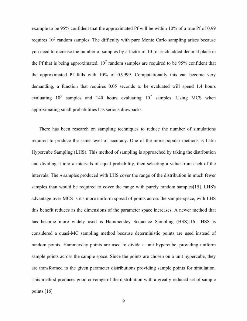
example to be 95% confident that the approximated Pf will be within 10% of a true Pf of 0.99
requires 105 random samples. The difficulty with pure Monte Carlo sampling arises because
you need to increase the number of samples by a factor of 10 for each added decimal place in
the Pf that is being approximated. 107 random samples are required to be 95% confident that
the approximated Pf falls with 10% of 0.9999. Computationally this can become very
demanding, a function that requires 0.05 seconds to be evaluated will spend 1.4 hours
evaluating 105 samples and 140 hours evaluating 107 samples. Using MCS when
approximating small probabilities has serious drawbacks.
There has been research on sampling techniques to reduce the number of simulations
required to produce the same level of accuracy. One of the more popular methods is Latin
Hypercube Sampling (LHS). This method of sampling is approached by taking the distribution
and dividing it into n intervals of equal probability, then selecting a value from each of the
intervals. The n samples produced with LHS cover the range of the distribution in much fewer
samples than would be required to cover the range with purely random samples[15]. LHS's
advantage over MCS is it's more uniform spread of points across the sample-space, with LHS
this benefit reduces as the dimensions of the parameter space increases. A newer method that
has become more widely used is Hammersley Sequence Sampling (HSS)[16]. HSS is
considered a quasi-MC sampling method because deterministic points are used instead of
random points. Hammersley points are used to divide a unit hypercube, providing uniform
sample points across the sample space. Since the points are chosen on a unit hypercube, they
are transformed to the given parameter distributions providing sample points for simulation.
This method produces good coverage of the distribution with a greatly reduced set of sample
points.[16]
9

1.4.2 Reliability Methods
Some of the early methods of analytical probabilistic analysis are the Mean Value (MV)
method, response surface method, and differential analysis[17]. All three methods are very
similar, the MV method and differential analysis methods are based on generating a taylor
series expansion of the response surface about the nominal values of the uncertain parameters.
With the MV method the moments of the approximate function are used to determine and
approximate Pf. The differential analysis method produces the taylor series expansion and then
partial derivatives of the response surface are calculated, helping to define the shape of the
response surface used to approximate Pf. The response surface methods are very similar to MV
methods, however; where the MV method finds a taylor series expansion of the true
performance function, the response surface approximates the performance function with a
simpler function, often a second order polynomial. After defining the simpler approximate
performance function, the response surface method proceeds the same as the MV method. An
in depth survey of reliability methods can be found in [14], [17].
First Order Reliability Method (FORM) and Second Order Reliability Method (SORM) are
methods that have come into much wider use in the past decade [18]. These methods are related
to the response surface method since response surface is approximated with a simpler function.
The goal of FORM is to compute failure probabilities efficiently, while avoiding the particular
errors due to problem formulation seen in other methods. The FORM method takes specific
advantage of transforming the problem into a standard normal space (u-space), where uncertain
parameters are independent with standard normal distributions. The uniformity and exponential
decay properties of u-space can be used to reduce error from response surface approximation as
well as simplifying the Pf calculation. The transformation and limit state approximation are the
10

basis of the FORM and SORM techniques. FORM approximates the limit state function with a
tangent hyper-plane, a linear or “First-Order” approximation, while SORM approximates the
limit state function with a Hyper-parabola, a “Second-Order” approximation. SORM can have
a dramatic effect of reducing error from limit state approximation, but it comes at the
computational cost of having to calculate derivatives of the limit state surface. Both FORM and
SORM are strong in regions of low probability, however the approximation error increases as
the limit state function nears the origin in standard normal space.
1.5 Probabilistic Analysis of SISO systems
A probabilistic view of Classical Control analysis for SISO systems will be a beneficial
step in providing information on performance of systems with parameter uncertainty. The goal
of this research is to show a probabilistic-based method for control systems analysis of SISO
systems with parameter uncertainty. The extreme conditions do not dominate the design
process by incorporating probability in the uncertainty. The most probable cases can be used to
achieve a desired performance while extreme cases can still be considered. The nominal
system, or system with mean values of all uncertain parameters, give one response but, a third
dimension to the traditional response plots is added when you add probability because each
response is represented with a distribution. Representing the probabilistic information on
classical response plots must be incorporated to provide clear understandable plots. One
method is the use of probabilistic confidence bounds.
1.5.1 Classical Response Analysis
Probabilistic response plot analysis looks at probabilistic analysis of the bode magnitude
and phase plots as well as the step response. With probabilistic response plots, the added
11

dimension of probability is used to give real confidence intervals that represent the range of
probable system responses. The idea pursued is to take these existing controls tools (bode, step
response) add to them the probabilistic analysis tools (HSS, FORM) providing a new capability
to evaluate system performance.
The hybrid approach developed mixes sampling and FORM to solve the problem. Using
both methods allows for the strengths of each tool to be used. Sampling computation is quick in
midrange probabilities and FORM approximation error is small in low probability regions. The
appropriate combination of the two methods can produce a cumulative distribution function
(CDF) of the system response with accurate representation through the middle and the tails of
the CDF. One advantage of mixing these methods in a hybrid approach is reduced
computational effort. As discussed in section 1.4.1 sampling alone can be extremely expensive
to reach low levels of probability. Using Form allows for specific computations of these much
lower levels of probability. A few FORM analyses can reach the levels of probability that
would require a number of samples many orders of magnitude larger. Once the full CDF has
been generated, it is easy to represent the desired confidence intervals for the system response.
12

A representation of probabilistic bode response is shown in Figure 1-4. If the Bode response is
considered to be probabilistic, a cross section of the response at any frequency would produce a
probabilistic distribution. Figure 1-4 shows the cross section of a specific frequency produces a
CDF representing the probability that the Bode response will be less than given magnitude or
phase values. A probabilistic step response would have the same structure, where at each
instant in time the response values of all possible systems could be represented as a
distribution.
-100
-80
-60
-40
-20
0
Mag
nitu
de (d
B)
10-1
100
101
102
-180
-135
-90
-45
0
Phas
e (d
eg)
Bode Diagram
Frequency (rad/sec)
0
0.5
1
Magnitude
Pr
0
0.5
1
Phase
Pr
Figure 1-4: Probabilistic Bode Response
Freq = 1.2 rad/sec.
CDF
CDF
Freq = 1.2 rad/sec.
13

1.5.2 Parameter Space Analysis
Parameter analysis examines how the parameter space affects the performance of the
system. The concept of the largest stable hypercube has been explored with norm bounded
uncertainty to determine how much certain parameters can change before becoming
detrimental to the system. The norm bounded set of parameters can be scaled until instability is
reached. This largest stable hypercube is simply the largest parameter space. By adding a
probabilistic distribution to the parameters not only can the largest stable hypercube be found,
but also the rate at which the probability of instability increases. For example, consider two
systems, system A parameters can be scaled by a factor of 2 with guaranteed stability.
However, continuing to increase the parameter scaling factor to 2.5 may lead to 30%
probability of instability. Now, system B is only stable when the parameter space is scaled by a
factor of 1.5, but a continued increase shows the parameters can be scaled to 2.5 with only 1%
probability of instability. System A may be considered more robust; however, if a small
probability of instability is acceptable, system B may be a much more desirable system.
Clearly, this information about the rate at which instability increases can only be obtained with
a probabilistic approach. Requirements would provide the method for choosing the most
desirable system. Parameter space analysis looks at this probability of instability problem as
well as how the size of the parameter space affects specific performance metrics.
The largest variation allowed in the parameters to still ensure stability is very useful. A
probabilistic approach to the analysis allows for the added depth of understanding how the
system will continue to perform if this largest variation is exceeded. Similar analysis can
provide added information to other performance metrics to determine how the changes in the
parameter distributions affect the performance characteristics. Items such as rise time, peak
14

value, and settling time of a step response can be analyzed to see how the mean of the
performance metric compares to the nominal value as the parameters space varies. Analyses
like these could aid in reducing costs of systems while maintaining a level of performance
characteristics and meeting a required level of risk.
This chapter has introduced the ideas of probabilistic controls and has presented a method
for approaching these types of problems. A hybrid approach to the problem was chosen to take
advantage of the strengths of both sampling and FORM methods. A full CDF of the system
response is desired, so with the hybrid approach FORM is used to resolve the tails, areas of low
probability, while Monte Carlo excels at filling in the mid regions of the CDF. The
development of the hybrid method and its benefits is presented. A review of sample problems
and a comparison of this analysis technique to current methods are presented next.
15

Chapter 2
Reliability Methods
2.1 Sampling and Monte Carlo
The Monte Carlo method is based on simulating a system with a set of sample points. A
sample is a vector or ordered set of the form x=(x1,x2,...xN), where N in the number of
uncertain parameters. This vector is a specific instance selected at random from the set of
random variables X. The most important part of the Monte Carlo method is generating the
sample points. Pseudo-Monte Carlo sampling, also known simply as Monte Carlo sampling
(MCS), is the most well known method. MCS consists of the pseudo-random number
generation of n samples on a k-dimensional hypercube. The ‘pseudo-’ implies that the random
numbers are produced with an algorithm intended to imitate a truly random natural process.
Random numbers may be repeated exactly given the seed used in the random number
algorithm. The “pseudo-” prefix may be dropped though it is still implied throughout this
paper. With MCS and many sampling methods, samples are generated over a uniform
distribution U(0,1), then inversely mapped the CDF of the desired distribution to produce the
desired samples. The approximation error (see section 1.4.1) when approximating an integral
when using Monte Carlo sampling is dependent on the even distribution of the sample points
not on the randomness [16]. With a limited sample size, purely random sampling can lead to
clumping of sample points or areas of the sample space not adequately represented. Uniformity
is key to efficient sampling techniques so alternate methods of generating sample points can
16

considerably improve the MC simulation results, two such methods are stratified sampling and
low discrepancy sampling.
2.1.1 Stratified Sampling Methods (Latin Hypercube)
The goal of stratified sampling techniques is to produce a more uniform distribution of
sample points throughout the sample space.[19] The basic concept is to divide the sample space
into bins of equal probability, and then generate a random sample inside of each unique bin. By
dividing the sample space into bins before selecting the random samples, better overall
coverage is achieved compared to MCS. Stratified methods also give the user the ability to
control the number of bins, ensuring a desired number of samples in given probability ranges.
One popular variant of the basic stratified sampling technique is Latin Hypercube sampling
(LHS). As a stratified technique, the sample space is again divided into unique bins of equal
probability, then a reduced set of samples are randomly selected in the sample space. With LHS
the randomly selected samples have two major constraints:
• each sample is randomly placed inside a bin
• all one dimensional projections of samples shall have one and only one sample in each
bin.
17
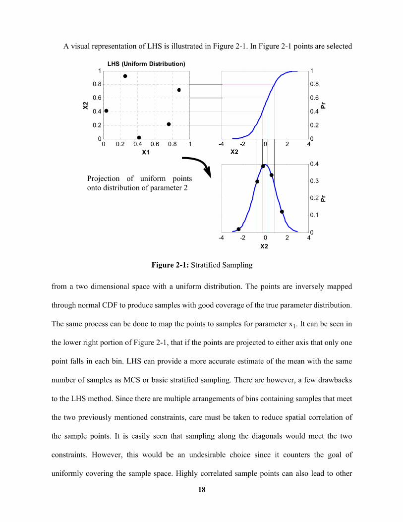
A visual representation of LHS is illustrated in Figure 2-1. In Figure 2-1 points are selected
from a two dimensional space with a uniform distribution. The points are inversely mapped
through normal CDF to produce samples with good coverage of the true parameter distribution.
The same process can be done to map the points to samples for parameter x1. It can be seen in
the lower right portion of Figure 2-1, that if the points are projected to either axis that only one
point falls in each bin. LHS can provide a more accurate estimate of the mean with the same
number of samples as MCS or basic stratified sampling. There are however, a few drawbacks
to the LHS method. Since there are multiple arrangements of bins containing samples that meet
the two previously mentioned constraints, care must be taken to reduce spatial correlation of
the sample points. It is easily seen that sampling along the diagonals would meet the two
constraints. However, this would be an undesirable choice since it counters the goal of
uniformly covering the sample space. Highly correlated sample points can also lead to other
0 0.2 0.4 0.6 0.8 10
0.2
0.4
0.6
0.8
1LHS (Uniform Distribution)
X1
X2
-4 -2 0 2 40
0.2
0.4
0.6
0.8
1
X2
Pr
-4 -2 0 2 40
0.1
0.2
0.3
0.4
X2
Pr
Figure 2-1: Stratified Sampling
Projection of uniform pointsonto distribution of parameter 2
18

less desirable results[19]. A third ‘soft’ criterion is included in LHS algorithms to minimize
correlation of sample points. One drawback of the LHS method is that the uniform quality of
the sample points decreases as the dimension k of the sample space increases, however; with
LHS the error of the estimate is still reduced compared to MCS with the same number of
samples, or similar results can be achieved with a fewer number of sample points.
2.1.2 Low Discrepancy Methods and Hammersley Sequence Sampling
Another class of sampling methods is quasi-Monte Carlo Methods[20], with the explicit
goal of producing an evenly distributed set of sample points over the sample space. The word
quasi- is used because the sample points contain no randomness, instead they are chosen by a
strictly deterministic algorithm. The goal again is to produce evenly distributed sample points
throughout the sample space, while not having a high correlation between the points, i.e. not
forming a regular grid. Another term for this type of method is low discrepancy sampling,
where discrepancy is a measure of how close the sample points are from an ideal uniform
distribution. This ideal uniform distribution can be thought of as a set of points that are all
equidistant from each other and unstructured, or have no regular pattern.
One variant of these quasi-Monte Carlo methods is Hammersley Sequence sampling (HSS)
described by Kalagnanam and Diwekar [16] which uses the Hammersley sequence to generate
n uniformly distributed samples on a k-dimensional hypercube. This low discrepancy method
has an advantage over techniques like LHS in that is selects points for uniformity over all
dimensions of the hypercube, where LHS primarily focuses on uniformity across one
dimension. HSS sample points keep their uniformity as the number of dimensions increases.
The differences in sampling techniques can be seen in Figure 2-2 showing the uniformity of the
19

HSS points. The benefits of the HSS method and the ability to get similar MC results with a
greatly reduced set of sample points led to the use of HSS points in all the sampling used in this
research.
Described in Kalagnanam [16] and Giunta [19], the Hammersley sequence is based on the
inverse radix notation using prime numbers as the radix- R. Radix notation of an integer p is a
sum of the digits of p multiplied by powers of the base, or radix.
(2.1)
for example in base 10 the number 516 in radix notation looks like,
. Reversing the digits of p about the decimal point generates a
0 0.5 10
0.5
1A) Randomly Generated Samples
0 0.5 10
0.5
1B) Latin Hypercube Samples
0 0.5 10
0.5
1C) Hammersly Sequence Samples
Figure 2-2: Monte Carlo Sampling Methods (100 points) A) Random Sample generation, B) Latin Hypercube Samples, C) Hammersley Sequence Samples.
p pmpm 1– …p1po=
p poRo p1R1 … pmRm+ + +=
516 6 100 1 101 5 102⋅+⋅+⋅=
20

unique fraction between 0 and 1, known as the inverse radix number, 0.615 in the case of the
example.
(2.2)
The Hammersley points of a k-dimensional hypercube are generated using
(2.3)
where Ri are the first k-1 prime numbers, and p=1,2,3...,N. These N Hammersley points are
distributed on the unit hypercube [0,1]k (see Figure 2-2c for a two dimensional representation).
Given the CDF of each parameter distribution the Hammersley points can be inversely
transformed to give a low discrepancy sequence of sample points in the parameter space.
2.1.3 Justification For Using HSS
A simple demonstration is given to show the benefits of low discrepancy sampling
techniques. Given a distribution with a known mean and variance apply each sampling method
and evaluate the mean and variance of the sample points. The level of Pr achievable with each
sampling technique is still 1/N. The benefit of LHS and HSS methods is the reduced error
bounds. The narrower error bounds result in a more accurate computation of the mean with the
same number of samples, or an equivalent mean calculation with far fewer sample points.
φR p( ) 0.pop1p2…pm=
φR p( ) poR 1– p1R 2– … pmR m– 1–+ + +=
xk p( ) pN---- φR1
p( ) φR2p( ) … φRk 1–
p( )=
21

Using a standard normal distribution, Figure 2-3 shows the results of 200 samples for different
sampling schemes. The more accurate representation of the HSS samples is evident. A
comparison of the mean and variance calculations can be seen in Table 2-1 and Table 2-2
respectively.These benefits of HSS drove the decision for the use of HSS in the methods
Table 2-1: Comparison of Mean Calculations for Different Sampling MethodsSampling Method 100 1000 10000 100000
MCS 0.00057607 0.0012104 2.1091e-005 6.9766e-005LHS 8.5421e-005 1.0392e-005 4.175e-007 9.8505e-008HSS 1.7347e-017 3.9248e-016 1.2248e-015 1.2098e-016
Actual mean value = 0
-4 -3 -2 -1 0 1 2 3 40
0.2
0.4
0.6
0.8
1 Random SamplesHSSActual
Figure 2-3: Comparison of Sampling Methods for a Standard Normal Distribution
Random Variable
Prob
abili
ty
22

developed. LHS showed a slight reduction in variance error however, the significant
improvement of HSS in the mean computation was the deciding factor for choosing HSS.
Being a deterministic set also allowed for easy repeatability of simulations.
2.2 First Order Reliability Methods (FORM)
Reliability methods are based on finding regions of failure and regions of safety of a given
system with uncertain parameters. Each random variable X is represented by a probabilistic
distribution. A scalar state function g(x) is defined which produces a metric of interest given a
specified set of the random parameters. This state function is used to separate the safe region
from the failure region, and is formulated so that g(x)>0 defines the safe region and
defines the failure region. The condition that separates failure and safety, g(x)=0, is know as the
limit state function. Probability of failure can then be defined by the integral shown in equation
(1.1) As mentioned before, with high dimensions this integral can be very difficult and
unmanageable. The ability to find the Pf without directly integrating the integral is highly
desirable.
The goal of FORM is to simplify integration by calculating Pf based on an analytical
approximation of the limit state function. These methods are especially effective when looking
at very low levels of probability of failure, where traditional sampling methods become
Table 2-2: Comparison of Variance Calculations for Different Sampling MethodsSampling Method 100 1000 10000 100000
MCS 0.93405 0.98866 0.99869 0.99968Error 0.06595 0.01134 0.00131 0.00032
LHS 0.93734 0.98960 0.99853 0.99981Error 0.06266 0.01040 0.00147 0.00019
HSS 0.93026 0.98886 0.99845 0.99981Error 0.06973 0.01113 0.00154 0.00019
Actual variance = 1
g x( ) 0≤
23

excessively expensive. Reliability methods simplify the problem of performing
multidimensional integration with a method of transforming the problem into a standard
normal space and approximating the limit state surface with a simpler lower order hyper
surface.
2.2.1 Transformation to Standard Normal Space
Standard normal space (u-space) is defined so that all random variables are statistically
independent, with normal distributions having zero mean and unit variance. In u-space all
random variables are defined by the standard normal density function.
[21] (2.4)
U-space has several desirable advantages for approximating the limit state surface. Most
notable are the exponential decay of the probability density, and the symmetry about the origin.
The exponential decay in the u-space allows for good approximations of Pf with a hyperplane
since the probability attributed to the area between the actual and approximate g(x) reduces
exponentially with the distance from the point where g(x) is approximated. Symmetry of u-
space simplifies the approximation because the direction to the hyperplane does not affect the
fU u( ) 1
2π( )1 2⁄-------------------
e 1 2⁄( )– uTu⋅( )⋅=
24

approximation only the distance. The transformation of the random variables to u-space, shown
in Figure 2-4, is the first step of the FORM process.
The transformation process takes the variables from their native distributions in the
physical space, x-space, through a one-to-one nonlinear mapping into u-space. The simplest
form, the Hasofer-Lind Transformation, can be used when the random variables X have normal
distributions and are uncorrelated. The normal distributions then must simply be shifted to a
standard normal distribution, by
(2.5)
For variables that are independent but not normally distributed the following diagonal
transformation may be used:
(2.6)
0 5 10 150
5
10
15x-space
x1
x2
-10 0 10 20-15
-10
-5
0
5
10
15
20u-space
u1
u2
Figure 2-4: Nonlinear Transformation from x-space to u-space
one to one mapping
Ui
xi µXi–
σXi
------------------=
ui Φ 1– FXixi( )[ ]=
25
Where is the standard normal cumulative distribution function (CDF) and is the CDF of
the random variable X. Transformations that are more complex exist to handle correlated
random variables, such as the Nataf and Roseblatt transformations. See reference [14] for a
review of these and other transformations. For the present research, only uncorrelated random
variables were used.
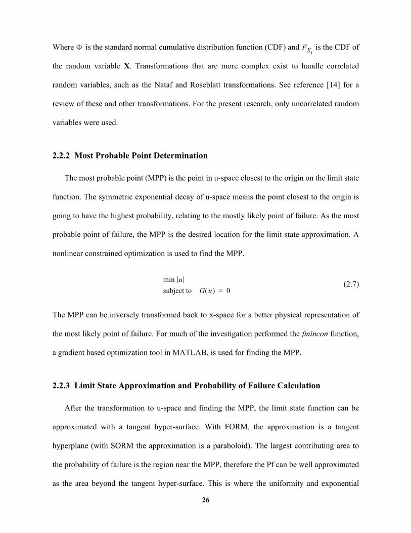
2.2.2 Most Probable Point Determination
The most probable point (MPP) is the point in u-space closest to the origin on the limit state
function. The symmetric exponential decay of u-space means the point closest to the origin is
going to have the highest probability, relating to the mostly likely point of failure. As the most
probable point of failure, the MPP is the desired location for the limit state approximation. A
nonlinear constrained optimization is used to find the MPP.
(2.7)
The MPP can be inversely transformed back to x-space for a better physical representation of
the most likely point of failure. For much of the investigation performed the fmincon function,
a gradient based optimization tool in MATLAB, is used for finding the MPP.
2.2.3 Limit State Approximation and Probability of Failure Calculation
After the transformation to u-space and finding the MPP, the limit state function can be
approximated with a tangent hyper-surface. With FORM, the approximation is a tangent
hyperplane (with SORM the approximation is a paraboloid). The largest contributing area to
the probability of failure is the region near the MPP, therefore the Pf can be well approximated
as the area beyond the tangent hyper-surface. This is where the uniformity and exponential
Φ FXi
min usubject to G u( ) 0=
26

decay of the normal distribution is helpful in reducing the significance of error in
approximation of the limit state hyper surface. SORM has the advantage of being able to reduce
error resulting from highly curved limit state function, however SORM comes with added an
complexity in calculating the Pf.
The Pf is approximated as the area on the failure side of the tangent hyper-surface. Since
FORM uses a tangent hyper-plane, the value of working in u-space is apparent at this point. As
seen in Figure 2-5, the Pf can be approximated with FORM simply using the distance from the
origin to the MPP. This distance is also known as the reliability index.
(2.8)
Finding the Pf for SORM is not quite as simple because you are approximating with a second
order hyper surface, however finding the area on the failure side of the surface is significantly
easier than finding the area of the failure region of the original g(x).
All FORM calculations were based on the MATPA tool developed at NASA Langley.
β
Pf Φ β–( )≈
Figure 2-5: Schematic of Limit State Approximation
u1
u2
β
mppU
G(u)=0
Failure Region
Accounts for most Pf
O
First order approximation of G(u)=0
27
Chapter 3
Hybrid Approach
The idea for using a hybrid method to approach probabilistic SISO analysis is to take
advantage of the strengths of two different techniques of reliability analysis. Sampling excels in
the central region of the probability distribution scale and FORM excels in end regions of the
probability scale, each technique is then used in its strong area. The data from this third
dimension of information is then used to provide information about the probable performance
of the system. The following sections describe a way to put these tools together to analyze the
effects of probabilistic parameter uncertainty on SISO systems.
3.1 General Hybrid Method
Given a control system with deterministic parameters, it will produce a single response
curve. For example, a Bode magnitude plot shows the magnitude of the system steady state
response due to a sinusoidal input over a range of frequencies. If slightly different parameters
for the system are applied, the Bode magnitude will obviously change. When the system
parameters are defined in a probabilistic manner, the system response will be probabilistic in
nature. In the example of Bode magnitude, at each frequency the magnitude can be represented
by a probabilistic distribution of the magnitude response of that frequency. A specific set of
parameters 'x' will produce a response C(x) at one frequency or time. The CDF of this response
can be thought of as giving the probability that the system response will be greater than some
28

reference level, C(x)>Ref. The approach to finding this distribution with reliability methods is
to write the limit state function as g(x)=Ref-C(x). Thus the failure region g(x)<0 is defined by
C(x)>Ref. Using reliability tools the full CDF can be found by sweeping across the full range
of reference levels between Pr[Ref-C(x)]=0 to Pr[Ref-C(x)]=1.
The shape of this response distribution is unknown so sampling is used as the first step of
the hybrid approach. HSS points are generated, then applied to the function C(x), producing a
first approximation of the response distribution. Using a low number of HSS points (e.g. 200)
allows for a good definition of the midrange of the CDF, including the general shape of the
distribution. Using sampling data to determine a starting point, FORM is used to resolve the
probability in the tails of the CDF down to a predetermined level. The hybrid method then takes
both sets of data and combines them to produce a full CDF of the system response at that
instance. The entire process must be repeated at each desired frequency or time to generate a
full probabilistic representation of the system response. Computational time obviously grows
with each additional instance for which the response CDF must be calculated, however; taking
advantage of matrix based operations in MATLAB can help to improve computational effort.
The sampling data can be computed over the full frequency range with one function call. The
FORM process involves a scalar optimization, which must be performed independently at each
frequency or time interval.
3.2 Tail Refinement Process
Sampling was used to find the midrange of the CDF, FORM is then used to refine the tail
regions of the CDF. The true CDF is unknown a priori, so the sampling data can be used to
determine a starting point for the FORM calculations. Given Pf=Pr[Ref-C(x)≤0] the C(x)
values from sampling can be used as the first initial Ref values for FORM. The first FORM
29

computation is performed at the fourth sample from each end of the CDF generated from
sampling to allow for an overlap between FORM and sampling data. Section 3.4 describes the
logic for choosing the 4th point, and the process for combining the sampling and FORM data.
Performing the FORM calculations at the location of the Ref value generated from a sample
evaluation guarantees a feasible problem with a known approximate solution. The FORM
problem becomes infeasible if the PF is zero, therefore feasibility is ensured because there
exists some level of probability of failure at this Ref value. When Pf=0 the limit state function
is mapped to infinity during the transformation to u-space. The optimization problem of
minimizing |u| subject to G(u)=0 is ill posed if no finite u can produce G(u)=0. Aside from
ensuring a feasible problem, performing the first FORM computation at a sample point allows
for a smart choice of initial conditions to be used for the optimization. The specific sample
point produced a value for the response function C(x), this reference value is then used in
FORM to solve . If the sample point produces C(x) and is then used as
the Ref value, the sample point x should be a good initial condition for finding an accurate first
form solution. Using the initial conditions that produced the reference condition aids in
reducing convergence time of the optimization.
Determining a step or value to the next FORM analysis is done using the slope of the
last three sample points. This technique places the second FORM point within the region of
sample points, again ensuring a feasible problem. The reference value is only moved a small
amount so the FORM problem is very similar to the first. The results of the first FORM
computation can be used as initial conditions for the second computation. Providing these
smarter initial conditions reduces the number of optimization iterations for the new FORM
calculation.
Pr g x( ) Ref C x( )–≤[ ]
∆Ref
30

At Each location of the SISO response analyses the FORM calculations are performed
many times, FORM computations are slow enough that only the desired number computations
to define the tail of the CDF should be calculated. With the shape and limit of the tail unknown,
it is difficult to evenly space the desired number of FORM calculations. It is known that the
CDF ranges from 0 to 1 on the y-axis so a vertical spacing can be defined and used to determine
the reference step size. For example, a FORM solution is desired at probability levels
decreasing by a factor of 10 (Pf=1e-2, 1e-3, e-4...). With the shape of the tail still unknown a
method for determining the reference step value for each new FORM computation must be
developed in an attempt to achieve the FORM results at the desired levels of probability.
The step determination method is slightly different for the first, second, and all remaining
steps. With no prior FORM data, the first step was chosen based on the average spacing of the
last three sample points. This averaging gives a rough estimate of the slope of the CDF tail, and
again ensures that a solution to the FORM problem exists since there is a known probability of
failure. A least squares fitting of data with extrapolation has been applied for determining the
remaining steps (2 - N). A review of many resultant CDFs showed a second order exponential
decay function best represented the tail of most CDF’s. For determining the second step only
two FORM calculations exist so a first order model, is used, where Pf is known
and the new x is desired. The step is then the difference between x at the desired Pf and the
previous x. For remaining steps, third and higher, calculations are done with the same least
squares method, however; using a second order exponential decay model, given as,
(3.1)
Pf a e⋅ b x⋅=
Pf a e⋅ b x⋅ ec x2⋅⋅=
31

where a, b, and c are coefficients of the fitted curve. Figure 3-1 shows the results of the
exponential decay extrapolation with asterisks representing predicted Pf at given locations
while the circles are the calculated Pf at that value. One modification was required for use of
the least squares technique, the x values must be normalized so that the least squares matrix in
equation (3.2) remains invertible as the x values become large.
(3.2)
Equation (3.2) represents the least squares equation used to find the coefficients of the
exponential decay function of equation (3.1). The coefficients are then used for the
extrapolation to find the new x value that will produce the desired probability.
-3.5 -3 -2.5 -2 -1.5 -1 -0.5 0
x 10-3
10-7
10-6
10-5
10-4
10-3
10-2
Normalized Scale Value
Pro
babi
lity
of F
ailu
re
Figure 3-1: FORM Step Prediction
∆Ref
Pf( )log 1 x x2a( )log
bc
⋅=
32

One of the primary reasons that this more elaborate extrapolation scheme was developed
was to prevent FORM from attempting zero probability computations. The FORM process uses
a transformation to standard normal space, when Pf is zero the distance to the MPP is infinite
since the limit state function is transformed to infinity. This event leads to an infeasible
problem. It is desired to avoid this scenario because in general FORM takes a significantly
longer time to not converge to a solution than it takes to converge. When FORM does not
converge it produces no beneficial information other than it did not work, the added
computational time makes this an undesirable scenario. A series of safeguards were developed
to avoid or limit the occurrence of failed FORM computations.
3.3 Capturing Abnormal Occurrences
FORM computations use a gradient based optimization, and are not guaranteed to produce
a solution. A few issues exist that can cause the optimization to not converge are as follows:
• Infeasibility of FORM (Pf =0 or 1)
• Limit state function discontinuities
• Nonsmooth limit state functions
• Complicated limit state functions requiring extensive function evaluations with given
initial conditions.
For these reasons, safeguards have been implemented into the algorithm to improve the
performance of the hybrid method. When the FORM computation fails before the desired level
of probability is reached, an attempt to alter specific conditions to find a converged solution is
desirable. With the goal of keeping computational time low, two safeguards were put in place
to attempt recovery from a failed FORM calculation. If the FORM computation fails,
determining if the problem is actually feasible is the primary step in finding a solution. If the Pf
33

is truly zero or one, the limit state function is transformed to infinity in u-space making the
FORM problem infeasible. A feasibility test uses a non gradient based optimizer to find the
closest point to the limit state function contained within the parameter space. A vector is
defined in u-space, from the origin to this point, then a set of samples along an extended portion
of this vector are transformed back to x-space. When evaluating these transformed samples, if a
sign change is found the problem is feasible, and if no sign change is found the problem is
considered infeasible. With feasibility of the problem known, there are two options. First, if the
problem is infeasible the initial conditions of the problem may not have been well suited for the
problem. New initial conditions are selected, half way between the infeasible and previous
feasible locations, and the FORM problem is computed again. If the second attempt also fails,
the hybrid analysis is not completed for that specific frequency, or time. The second option
when FORM is found to be not feasible then the reference value is outside the possible
response range and must be stepped back. A new reference value is chosen half way between
the failed and previous successful computations. As before this is only attempted once to
facilitate the quick computation for the entire response. The individual issues that cause the
FORM failures can be scrutinized separately if the information at that specific frequency or
time is needed.
3.4 Hybrid Data Processing and Representation
After sampling and FORM computations, probability of failure data exist for each
respective method. These two sets of data must be combined to form one continuous
monotonically increasing CDF. Both Methods are approximations and may not exactly match,
therefore, FORM and Sampling data overlap in the hybrid method helping facilitate a smoother
combination of the data. For FORM, approximation error increases in u-space as the limit state
34

function approaches the origin. A probability of failure level of 2% was assumed as an upper
limit for trusting FORM solutions. Above this level of probability the approximation error is
likely to be significant. However, sampling is more accurate when there are a significant
number of points in the failure region compared to the total number of samples evaluated.
Sampling results with less than 2% of the samples in the failure region were assumed less
accurate than a FORM solution at that probability level. For this research 200 sample points
were typically used, so less than 5 was considered not as accurate as FORM. The reasoning
behind the transition between FORM and sampling is based on an assumption of when to trust
FORM and when to trust sampling. The data combination logic was defined to achieve a
transition between FORM and sampling, using a few safeguards to ensure a smooth and
monotonically increasing final CDF. Logic must be specified for the combination when the
points don’t exactly line up. The logic used is as follows:
• The end 4 points of the sampling are discarded due to lack of accuracy.
• If all FORM points have a Pf less than the 5th sample point from end of the CDF, they
are appended to the sampling Pf vector.
• If any FORM points result in PF greater than the 5th sample point from end of the CDF,
they are discarded and the remaining points are appended to the Pf vector.
The 5th sample point from the end is assumed as the limit between when FORM is trusted and
where sampling is trusted. The assumed limit is the justification for discarding FORM points
greater than this 5th sample point from the end of the CDF. The combination logic is used for
both tails of the CDF, and is necessary to insure a proper CDF.
One of the desires of generating the data to produce a full CDF of the system response is the
ability to calculate the mean and variance of the system response. Both pieces of information
35

are very useful in the analysis of SISO systems. Depending on the distributions of the
parameters and the characteristics of the system the mean response may or may not follow the
response of the system with nominal parameter values. Representing the spread of the CDF, the
variance can also be useful if comparing multiple systems to determine which system will have
the narrowest range of responses. Given the relation between the CDF and the PDF
(3.3)
where F(x) is the CDF and f(x) is the PDF. The expected value is calculated using the CDF data
as follows.
(3.4)
Similarly the variance is calculated in the following equation.
(3.5)
Representing the entire distribution along with the system response is unwieldy and
difficult to interpret, leading to a method of representing the response by its mean, upper, and
lower confidence bounds. The confidence bounds represent some percentage of system
responses will be within these bounds.
The data from both methods (e.g. sampling and FORM) representing the CDF are discrete,
and will not likely have a datum point exactly coinciding with the desired confidence interval.
Thus, the data must be curve fitted to interpolate where the probability limit lies. A spline
interpolate works poorly because of the generated CDF data lacks smoothness, which produces
overshoot in the interpolate. By definition monotonicity must be maintained since the CDF is
f x( ) F x( )dxd
--------------=
E[ ] x f⋅ X x( ) xd∞–
∞
∫ x Fd X x( )⋅
0
1
∫= =
V[ ] x E[ ]–( )2 fX x( ) xd⋅
∞–
∞
∫ x E[ ]–( )2 Fd X x( )⋅
0
1
∫= =
36
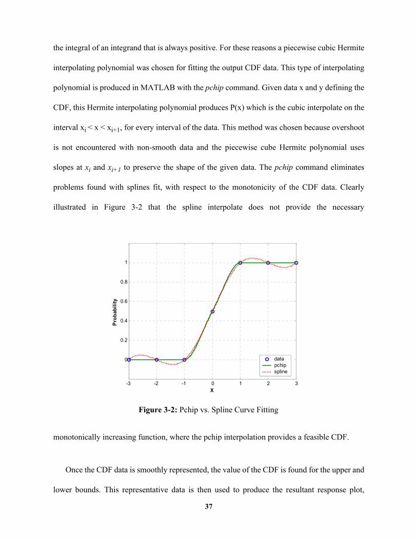
the integral of an integrand that is always positive. For these reasons a piecewise cubic Hermite
interpolating polynomial was chosen for fitting the output CDF data. This type of interpolating
polynomial is produced in MATLAB with the pchip command. Given data x and y defining the
CDF, this Hermite interpolating polynomial produces P(x) which is the cubic interpolate on the
interval xi < x < xi+1, for every interval of the data. This method was chosen because overshoot
is not encountered with non-smooth data and the piecewise cube Hermite polynomial uses
slopes at xi and xi+1 to preserve the shape of the given data. The pchip command eliminates
problems found with splines fit, with respect to the monotonicity of the CDF data. Clearly
illustrated in Figure 3-2 that the spline interpolate does not provide the necessary
monotonically increasing function, where the pchip interpolation provides a feasible CDF.
Once the CDF data is smoothly represented, the value of the CDF is found for the upper and
lower bounds. This representative data is then used to produce the resultant response plot,
-3 -2 -1 0 1 2 3
0
0.2
0.4
0.6
0.8
1
X
Prob
abili
ty
datapchipspline
Figure 3-2: Pchip vs. Spline Curve Fitting
37

whether it is a Bode response or a step response. Having the fully defined CDF also allows
quick representation of the response with any other desired confidence intervals without having
to regenerate the response.
3.5 Response Analysis Issues
The hybrid method of response analysis works for a wide range of systems. In general,
good performance is achieved but the automated method of performing FORM calculations
does not guarantee finding probability levels to the desired limits. FORM does provide a
benefit to defining the CDF but also possesses it’s own difficulties. One issue arises from using
an exponential decay model when extrapolating the tails of the CDF and determining a .
If the tail of this CDF does not fit the model, the extrapolation technique may perform poorly
preventing a converged FORM solution. An example of this occurs when using uniform
distributions for the uncertain parameters. The often sharp drop off in probability of the
response CDF makes the exponential decay model less efficient and may miss the point where
the probability drops suddenly. An unknown shape of the CDF tails and a large possibility of
response distributions means any extrapolation method is unlikely to perform well in all cases.
One solution to this problem may be the inverse MPP problem, instead of choosing a Ref value
and finding the Pf with FORM, the Pf could be given and perform an inverse problem to find
the Ref value that produces the chosen Pf. This would eliminate any extrapolation technique
because desired levels of Pf would be able to be exactly chosen. No research has been
performed on this problem, so the inverse MPP approach remains as future work.
A second issue causing difficulty for the hybrid method originates with the FORM process.
There are cases where the Pf reduces, although the MPP does not move significantly farther
away from the origin in u-space. With multiple FORM calculations performed to develop the
∆Ref
38

end of the CDF, the limit state function normally moves farther from the origin with each new
calculation. The FORM process uses a first order approximation of the limit state function so
the probability of failure is found directly from the distance the MPP is from the origin.
Equation (1.1) showed that Pf is found by integrating over the failure region, therefore the Pf is
reduced when this area is smaller even if the MPP does not move farther from the origin, in u-
space. If the MPP does not move significantly farther from the origin, the reduction of
probability is not captured by FORM and the approximation error increases. An example of this
is illustrated in Figure 3-3, where the approximated Pf stays constant as the limit state function
shifts from G1(u) to G2(u). As FORM is calculated at each different location, the limit state
function increases its curvature instead of moving away from the origin. Occasionally seen in
Bode magnitude plots around the system poles, FORM calculations may never reach the
desired limit if the MPP does not shift away from the origin in u-space. The implementation of
SORM has the potential to improve accuracy in probability of failure calculation by reducing
the error in approximation of the highly curved limit state function.
Figure 3-3: First Order Approximation Problem
u1
u2
mpp
G2(u)=0G1(u)=0
Tangent Surface
O
39

An issue that can lead to limited low probability computations of a CDF is found when the
limit state function becomes non-smooth or highly erratic. This issue is particular to the use of
a gradient based optimizer in the FORM process, not the overall FORM concept. Having many
minimums or sharp edges in the limit state function can prevent the gradient-based FORM
optimization from converging to a solution, or converging to the correct solution. Designed as a
general tool for system analysis, the hybrid method cannot accommodate or work around all of
these issues. Most difficulties can be determined from the resulting information of the overall
analysis. Adjustments to the developed method for specific problems can often solve these
issues, so that full CDF's to the desired level of probability may be achieved.
The last difficulty is specific to phase representation and is not just a problem with the hybrid
method. If the variation in the uncertain parameters causes the phase response to range greater
than 2π, producing a representation of the CDF becomes difficult. The current process
developed does not have the ability to accommodate a CDF that spans a range greater than 2π.
3.6 Extending to Parameter Space Analysis
While probabilistic response plots analyzed a specific set of distributions, parameter space
analysis is the concept of looking at how large the uncertain parameters can be allowed to
expand, before undesirable system metrics occur. The parameter space is defined for this work
as, the hypercube containing all possible combinations of the uncertain parameters. The
standard approach finds the amount parameters can expand before undesirable metrics are
found. Approaching this analysis probabilistically allows the parameter space to be expanded
beyond the first undesirable metric, finding the probability that undesirable performance
metrics will occur. For the stability example, if this hypercube is allowed to expand beyond the
onset of instability the growth rate of probability of instability can be measured. This can give
40

an insight to the allowable range of parameters for a predefined acceptable probability of
instability and an indication of the robustness of the system. The basic concept of the hybrid
method is the same however the approach or application is different between the probabilistic
response plots and the parameter space analysis. Two types of parameter space analysis are
explored, performance metric analysis and probability of instability analysis. The performance
metric technique most closely follows the process used in the probabilistic response plots,
while probability of instability analysis shares the same basic tools, but the approach is
different.
3.6.1 Performance Metric Analysis
Few modifications were necessary to adapt the system response hybrid techniques to
analyze parameter space with respect to performance characteristics. Given the full set of
uncertain parameters (parameter space) and a performance metric, a CDF of all possible
performance metric results can be found. Sampling and FORM are used in the same way as
described in sections 3.1 - 3.4. HSS samples are used to give a quick approximation of the
performance metric CDF midrange. In this case C(x) is the function that generates the desired
performance metric; rise time, peak value, or settling time. Using the sampling as a reference,
FORM is used to finish generating the CDF with the limit state function again defined as
g(x)=Ref-C(x). 'Ref' is a value used to step away until the low level of probability is reached.
This full CDF now describes the range and likelihood of the performance metric results.
Instead of performing the computations of another time or frequency as in the probabilistic
response plots, the size of the parameter space is increased and another performance CDF is
generated. The mean and variance of these CDFs are computed and then compared with the
41

performance of the nominal system. A new specific performance metric function J, has been
defined in this research. The expected value of J or the variance of J is compared to the
performance metric of the nominal system, Jo, in a simple ratio, E(J)/Jo or V[J]/Jo. Plots of
these two ratios can provide information about how expanding the parameter space, increasing
the amount of uncertainty, affects the performance metric defined by J.
3.6.2 Probability of Instability Analysis
As a parameter space analysis tool, stability analysis is very different from the performance
metric analysis. The main difference when looking at probability of stability is that a full CDF
is never desired. The performance metric analysis finds a full CDF of the metric at each
increasing amounts of uncertainty. In probability of instability analysis, if the failure region is a
closed space, the probability of instability may never reach a value of one. This difference is
the reason that the approach is so different between the two parameter space analyses.
The basic concept is; given a system with some nominal parameter values, how much
uncertainty can be allowed before instability is possible in the system. Allowing for
probabilistic definitions of the uncertain parameters lets the analysis be taken a step further
than conventional approaches to determining stability bounds, where the rate at which
probability of instability increases can be determined. It is desired to explore how the parameter
space can be enlarged before instability onset changes depending on the shape, or scaling
factor, of the increasing parameter space. Largely dependent on how much is known about the
42

parameter uncertainty, there are many ways to scale this hypercube of the parameter space.
Four such methods are considered;
• Uniform percentage of mean values,
• Ratio based on the most probable point of failure in x-space (mppX),
• Ratio based on the closest point on g(x)=0 to the nominal values,
• Ratio based on the gradient of g(x).
These are discussed next.
Each method is trying to find the probability of instability based on the size of the parameter
space, but each is different on how they select the relative scaling between each side of the
hypercube. The last three scaling methods are illustrated in Figure 3-4.
The first method explored was the uniform percent scaling of the mean values. This was
chosen as it appears the most common amongst non-probabilistic parametric uncertainty
Figure 3-4: Hypercube Scaling Methods
x1
x2
g(x)=0
mppX
Min|µ-x|
Gradient Vector
43

analysis. Each parameter is defined as the range where is the mean, or
nominal value. This generates a norm bounded set or uniform distribution with all values
having equal likelihood. Using a simple uniform distribution does not show the probabilistic
benefits, however; it allows for comparison with previous works. The analysis can easily
incorporate distribution information when known. The process is the same when using
distributions with bounded support with the shape only affecting the calculated probability
levels. The largest stable hypercube is initially unknown so sampling is used to find a rough
guess of when the parameter space produces unstable systems. A very small amount of
uncertainty is allowed then 200 HSS samples are evaluated to check stability. The size of the
hypercube is increased until probability of stability is no longer 100%. Having bounded the
transition between zero probability of instability and non-zero probability of instability, a
bisection technique is used with HSS sampling to find a hypercube producing a low probability
of instability. After narrowing down the probability, FORM computations are performed at
steps down to a low level of probability of instability. These FORM calculations provide the
data for representing how the probability of instability increases as the parameter space
increases.
A second method for scaling the hypercube is to find the most probable point of failure in
x-space, MPP in x-space, and let the vector from the mean values to the MPP in x-space be the
vector to one corner of the hypercube, see Figure 3-4. This method requires some general
knowledge about the parameter distributions, not just the mean value. The parameter space is
first set very large, though still with the given distribution shapes. A FORM analysis provides a
MPP in x-space used to define the new scaling ratio. This method has the benefit of knowing
exactly what parameter space range will be the largest stable hypercube. Using the MPP in x-
ηi 1 ηi∆±( )⋅ ηi
44

space as the scale for the hypercube ensures that the hypercube will touch the limit state
function first at this point. The hypercube be can slightly increased with this scaling,
performing FORM calculations as it grows to find probability of instability.
The previous two methods assumed some previous knowledge of the uncertain parameter
distributions. Transformations to u-space require knowledge of the uncertain parameter
distributions, however, basic information of the parameter distributions may be unknown. One
way to determine a hypercube scaling factor without this knowledge is to work in x-space. The
closest point to the nominal parameter values on the limit state function, g(x)=0, is found and
used to set the scaling ratio of the hypercube, see Figure 3-4. This closest point is found from
the following constraint equations, where η is again the nominal parameter value.
(3.6)
This minimum distance point in x-space, similar to MPP in x-space method, gives the largest
set of parameters with this scaling that will maintain stability. The parameter space hypercube
is then increased from this starting size using FORM to see how the probability of instability
increases as the hypercube grows.
The final technique used for developing a hypercube scaling was to use gradient
information of the state function, where the ith hypercube element can be written as,
(3.7)
A finite differencing approach was used to find the gradient information of the limit state
function seen in equation (3.7). This finite differencing was done using as the difference
between 95% and 105% of the nominal value of xi. Unlike some methods, it is not immediately
min η x–subject to g x( ) 0=
∇i g( ) g∂xi∂
------- ∆g∆xi--------≈=
∆xi
45

known what range of parameters will first introduce instability using this method of
determining hypercube scaling. The gradient information gives a vector that points in the
direction the greatest rate of change in g(x). Points are selected along the direction of this
vector until a sign change is g(x) is found, indicating the transition into the failure region. A
bisection technique can be used to find a more precise value for the point on the limit state
surface. From this point FORM can be used to find the probability of instability in a similar
way as the previous methods.
Each of these scaling methods will provide the largest parameter values allowable, given
that scaling factor, that ensure 100% stability. The additional probabilistic information can give
insight to how quickly the probability of instability in the system grows when these limiting
values are exceeded.
46

Chapter 4
Analysis of Hybrid Method
4.1 Definition of Example Problem #1
Two different example problems on uncertainty analysis were chosen from the literature to
compare with the newly developed hybrid method. The first example, developed by Wise
[22][7][23], is a missile pitch autopilot system with four uncertain parameters. The following
aerodynamic equations and nominal aerodynamic stability derivatives represent a trim angle-
of-attack of 16 degrees, Mach 0.8, and altitude of 4000 ft. With a linearized set of equations,
the pitch dynamics decouple from the roll-yaw dynamics of the missile system. The state space
representation of the pitch dynamics is,
(4.1)
where α is angle-of-attack, q is pitch rate, δe is elevon fin deflection. The uncertain parameters
are the dimensional aerodynamic stability derivatives with the following nominal values used:
Zα=-1.3046 (1/s), Zδ=-0.2142 (1/s), Mα=47.7109 (1/s2), and Mδ=-104.8346 (1/s2). The
corresponding accelerometer and gyro output equations are,
(4.2)
α·
q·Zα 1
Mα 0αq
Zδ
Mδ
δe+=
Az
q
VZα 0
0 1αq
VZδ
0δe+=
47

where Az is normal body acceleration and V is velocity. Having a damping ratio of ζ=0.6 and
natural frequency of ω=113.0 (rad/s) the dynamics of the elevon fin actuator are governed by
equation (4.3), where is the commanded elevon deflection.
(4.3)
Incorporating the actuator dynamics the linearized missile dynamics can be represented in the
following transfer function.
(4.4)
See reference [23] for a full development of the system.
A classical autopilot structure is given to control the commanded elevon fin deflection, δec,
based on the normal body acceleration and pitch rate outputs. A block diagram of the system
with the two controller blocks is given in Figure 4-1. The two controllers have the following
δec
δ··e 2ζωδe·– ω2δe– ω2δec+=
G s( )
ω2V Zδs2 ZαMδ ZδMα–+( )
s2 Zαs– Mα–( ) s2 2ζωs ω2+ +( )----------------------------------------------------------------------------------
ω2 Mδs MαZδ MδZα–+( )
s2 Zαs– Mα–( ) s2 2ζωs ω2+ +( )----------------------------------------------------------------------------------
Azδec-------
qδec-------
= =
Inner Rate Loop
Outer Accel. Loop
( )a zK s as+ q
δzA
q( )q qK s a
s+
G(s)K(s)
AzAzc
Figure 4-1: Classical Pitch Autopilot
48

values: Ka=-0.0015, Kq=-0.32, az=2.0, and aq=6.0. The overall system provides the normal
body acceleration, Az, in response to an acceleration command. This missile pitch system
allowed the hybrid method to be compared to the analysis done by Wise[23]. The original
papers [22][7][23] did not use a probabilistic representations of these parameters, however
assumed distributions were given to each of the parameters. All four uncertain parameter was
assumed to have a beta distribution having shape coefficients of 2 and 2 with limits of plus and
minus 50% of the nominal value.
4.2 Probabilistic Response Plots
The Bode and step response analysis were explored first, with the missile pitch problem.
Some results of the hybrid method producing probabilistic response plots are shown in this
section. The performance of the hybrid method was also analyzed. One hybrid method analysis
was looking at the benefits of the hybrid approach when calculating the mean and variance of
the distributions. The hybrid approach was also compared with a standard -analysis
technique.
4.2.1 Bode Analysis
The Bode response provides information about how physical system responds to sinusoidal
inputs over a range of frequencies after all transients have died out[24]. Introducing
probabilistic information into this classical analysis tool can expand the benefits of this
analysis, showing what frequency ranges are most affected by the parametric uncertainty.
Frequency response techniques such as Bode analysis must represent both parts of the complex
data, magnitude and phase. Because the FORM process is optimizing a scalar output the two
portions of the complex data must be analyzed separately, forcing Bode magnitude and phase
µ
49

plots to be generated separately with the hybrid method. Using the missile pitch autopilot
system described in section 4.1, probabilistic Bode magnitude and phase responses can be seen
in Figure 4-2. The hybrid method propagated the parametric uncertainty through the system
providing a full distribution of the magnitude and phase at each frequency. Representing this
probabilistic information in the traditional Bode plot without adding a third axis produces
cluttered and difficult to read graphs, as mentioned in section 3.4. The probabilistic information
in Figure 4-2 is represented by the mean, upper, and lower confidence intervals. This technique
simplifies representation of the data to produce a clean readable plot. For this analysis,
10-2
100
Frequency ω (rad/s)
Mag
nitu
de d
B
Magnitude
10-1
100
101
102
103
104-400
-300
-200
-100
0
Frequency ω (rad/s)
Phas
e (d
eg)
Phase
Lower IntervalMeanUpper Interval
Lower IntervalMeanUpper Interval
Figure 4-2: Probabilistic Bode Analysis
50

confidence bounds of 99.999% are represented, which means 99.999% of all responses will be
below the upper bound and 99.999% of the responses will be above the lower bound. Although,
only one set of bounds is displayed, the entire CDF has been calculated, therefore confidence
bounds of any level less than the FORM computation limit can be displayed without
reanalyzing the system. Viewing the results seen in Figure 4-2 shows the system is always
stable with the assumed distributions on the parameters.
4.2.2 Step Response Analysis
Similar to the Bode Response Analysis, a probabilistic step response provides information
not found with norm-bounded uncertainty techniques. The hybrid method does not change
when applied to the step response; only the limit state function is different. The limit state
function that represents the step response of the system is evaluated at individual time intervals
in the same style as the probabilistic bode response. This probabilistic step response of the
51

missile pitch problem can be seen in Figure 4-3. The variance is calculated, along with the
mean and confidence intervals, for all the points of the response. The mean and variance of the
response are only available with a probabilistic representation of the response plots. This
probabilistic step response depicts areas that are more affected by the uncertainty. The first 0.5
seconds for example have a large variation in response while the variance drops as the system
reaches its steady state value.
4.2.3 Comparing the Hybrid Method with Standard Uncertainty Analysis
Verification that the hybrid method is indeed producing accurate results requires that it be
compared with an existing method for uncertainty analysis. It was stated earlier that the
0 0.5 1 1.5 2 2.5 3 3.5 4 4.5-0.5
0
0.5
1
1.5
time (sec)
outp
ut
0 0.5 1 1.5 2 2.5 3 3.5 4 4.510
-6
10-4
10-2
time (sec)
Varia
nce
Lower IntervalMeanUpper Interval
Figure 4-3: Probabilistic Step Response
Out
put
Varia
nce
52

standard uncertainty analysis and design methods in controls, µ-analysis and , are
dominated by ‘worst-case’ scenarios, essentially the vertices of the parameter hyperspace.
While this technique neglects considerations of likelihood of the response, it is useful to
compare the hybrid method to this standard procedure. Giving all parameters uniform
distributions to define the uncertainty allows the hybrid method to be compared directly to the
current standard of a delta block representation of the uncertainty (see Figure 1-3). The delta
block representation is the current basis for most uncertainty analysis which does not produce
probabilistic information, however the two different methods should produce the same bounds
for the system response. Figure 4-4 shows the resulting comparison of the Bode magnitude
analysis of a simple mass-spring-damper problem. It can be seen that the hybrid method
H∞
10-1
100
10110
-3
10-2
10-1
100
101
Frequency ω (rad/s)
Mag
nitu
de d
B
Figure 4-4: Hybrid Method Compared to ∆ Block Representation of Uncertainty
53
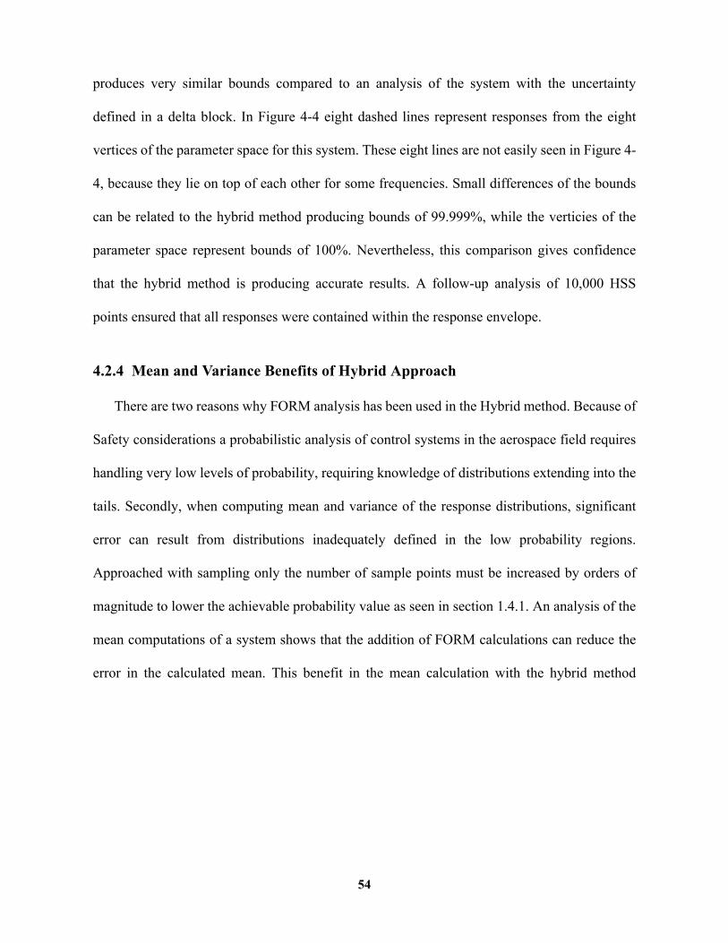
produces very similar bounds compared to an analysis of the system with the uncertainty
defined in a delta block. In Figure 4-4 eight dashed lines represent responses from the eight
vertices of the parameter space for this system. These eight lines are not easily seen in Figure 4-
4, because they lie on top of each other for some frequencies. Small differences of the bounds
can be related to the hybrid method producing bounds of 99.999%, while the verticies of the
parameter space represent bounds of 100%. Nevertheless, this comparison gives confidence
that the hybrid method is producing accurate results. A follow-up analysis of 10,000 HSS
points ensured that all responses were contained within the response envelope.
4.2.4 Mean and Variance Benefits of Hybrid Approach
There are two reasons why FORM analysis has been used in the Hybrid method. Because of
Safety considerations a probabilistic analysis of control systems in the aerospace field requires
handling very low levels of probability, requiring knowledge of distributions extending into the
tails. Secondly, when computing mean and variance of the response distributions, significant
error can result from distributions inadequately defined in the low probability regions.
Approached with sampling only the number of sample points must be increased by orders of
magnitude to lower the achievable probability value as seen in section 1.4.1. An analysis of the
mean computations of a system shows that the addition of FORM calculations can reduce the
error in the calculated mean. This benefit in the mean calculation with the hybrid method
54

(shown in Figure 4-5) is similar to increasing the number of sample points by a factor of 100.
The comparison analysis in Figure 4-5 shows the error in the mean computations of a Bode
phase analysis in the spring mass system (section 4.2.3) with three uncertain parameters. An
analytic result for the exact mean is not available, an assumed ‘true’ answer was found from a
Monte Carlo simulation with 300,000 samples. The mean response at each frequency was then
calculated using a trapezoidal integration technique for solving equation (3.4). Three cases; 200
HSS, 10,000 HSS, and the hybrid approach, were performed and the mean values of the
response were calculated. Figure 4-5 shows the difference between these cases and the
accepted value . The comparison shows how adding
FORM results on the tails of the distributions generated by 200 HSS points improves the mean
10-1
100
101
10-6
10-5
10-4
10-3
10-2
Frequency ω (rad/s)
10,000HSS - 455.8Hybrid - 384.05200HSS - 5.93
Figure 4-5: Mean Computation Error for Hybrid and HSS Methods
acce
pted
mea
n c–
alcu
late
d m
ean
acce
pted
mea
n----
--------
--------
--------
--------
--------
--------
--------
--------
--------
--------
--------
--
accepted mean c– alculated meanaccepted mean
----------------------------------------------------------------------------------------------
55
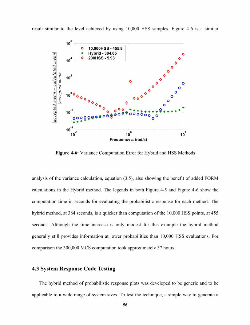
result similar to the level achieved by using 10,000 HSS samples. Figure 4-6 is a similar
analysis of the variance calculation, equation (3.5), also showing the benefit of added FORM
calculations in the Hybrid method. The legends in both Figure 4-5 and Figure 4-6 show the
computation time in seconds for evaluating the probabilistic response for each method. The
hybrid method, at 384 seconds, is a quicker than computation of the 10,000 HSS points, at 455
seconds. Although the time increase is only modest for this example the hybrid method
generally still provides information at lower probabilities than 10,000 HSS evaluations. For
comparison the 300,000 MCS computation took approximately 37 hours.
4.3 System Response Code Testing
The hybrid method of probabilistic response plots was developed to be generic and to be
applicable to a wide range of system sizes. To test the technique, a simple way to generate a
10-1
100
10110
-4
10-2
100
102
104
106
Frequency ω (rad/s)
10,000HSS - 455.8Hybrid - 384.05200HSS - 5.93
Figure 4-6: Variance Computation Error for Hybrid and HSS Methods
acce
pted
mea
n c–
alcu
late
d m
ean
acce
pted
mea
n----
--------
--------
--------
--------
--------
--------
--------
--------
--------
--------
--------
--
56

large number of different uncertain test systems was needed. This scalable test system
generates stable transfer functions with an arbitrary number of random variables. The scalable
testing model was used both for systematic testing of the hybrid method and for computational
effort analysis.
4.3.1 Scalable Testing Techniques
The scalable model is built using the real portion of the system poles as random variables.
Using the poles as the basis for the random variables was done both for simplicity and for
producing systems of similar style while they were scaled. The technique developed starts by
using the rmodel function in Matlab to define a random stable transfer function. Considering
complex conjugate pairs as one variable the real component of each pole is given a
probabilistic distribution. All distributions were lognormal, with the nominal pole value used as
the mean, and a standard deviation defined by 10% of the pole value. Although all poles are
defined by lognormal distributions, using the pole value in determining the standard deviation
gave a wide range of distribution shapes. The order of the system transfer function could now
be arbitrarily set, thereby quickly producing systems of order n. Since there are an unknown
number of conjugate pairs, the number of random variables is less than n. This drawback of
basing the scalable model off the rmodel function is that the number of random variables
cannot be directly specified. While the number of poles is specified, an unknown number of
complex poles will cause some variation in the number of random variables. Nevertheless, this
scalable model allowed for extended testing of the hybrid software to ensure it wasn’t overly
specialized for the few specific example problems being analyzed.
57

4.3.2 Computational Effort Analysis
One of the main benefits of the scalable testing model was the ability to generate an
extensive computational effort analysis relating the CPU time with the number of uncertain
variables. Figures 4-7 through 4-9 show the computational time in minutes for an increasing
number of uncertain parameters. The time represented is the time necessary to complete a full
Bode magnitude or phase response plot using the hybrid method evaluated at 20 evenly space
frequencies. Some variation is expected even in systems with the same number of random
variables since the exact number of FORM calculations cannot be specified, therefore the
number of FORM computations at each frequency is not the same. This computation analysis is
meant to look at the trend of the hybrid method computing a full system response. The
computation time as a function of the number of random variables is depicted in Figure 4-7.
Fitting a second order polynomial through the data points shows the apparent second order
growth trend in CPU time. For the Bode magnitude data seen in Figure 4-7 the norm of the
0 5 10 15 20 25 30-2
0
2
4
6
8
10
12
14
16
18
Number of Random Variables
Com
puta
tion
Tim
e (m
in)
data 1 linear quadratic
Figure 4-7: Bode Magnitude Computational Time Analysis
58

residuals for the fitted data was 8.8 for the linear fit and 6.3 for the quadratic curve fit. It
becomes evident that as the number of random variables increases the computational effort will
eventually become prohibitively costly. The complexity of the limit state function is also a
major contributor to the computational time. While a more complicated limit state functions
increase computational time, the second order growth remains evident. This can be seen in the
difference between time analysis of the Bode magnitude and Bode phase plots. The
computational effort for the Bode phase plot is depicted in Figure 4-8, it can be seen that the
data has a similar quadratic curve as Figure 4-7, however; the phase plot computations are
faster. For the Bode phase data, the norm of the residuals was 3.2 for the linear fit and 1.7 for
the quadratic fit. The step response is a more complicated function to evaluate than either the
Bode magnitude or phase, thus it is expected to require more computation time. Illustrated in
0 5 10 15 20 25 30-2
0
2
4
6
8
10
12
Number of Random Variables
Com
puta
tion
Tim
e (m
in)
data 1 linear quadratic
Figure 4-8: Bode Phase Computational Effort Analysis
59
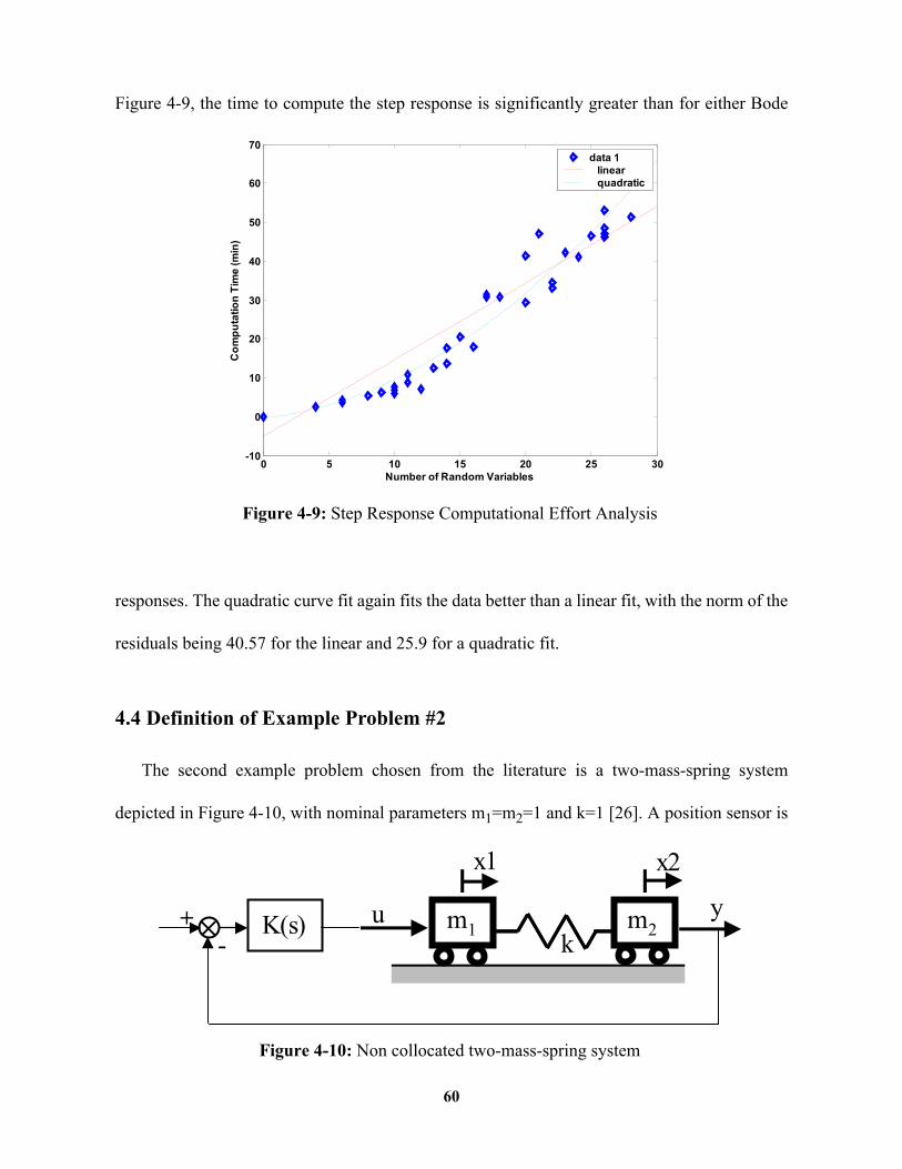
Figure 4-9, the time to compute the step response is significantly greater than for either Bode
responses. The quadratic curve fit again fits the data better than a linear fit, with the norm of the
residuals being 40.57 for the linear and 25.9 for a quadratic fit.
4.4 Definition of Example Problem #2
The second example problem chosen from the literature is a two-mass-spring system
depicted in Figure 4-10, with nominal parameters m1=m2=1 and k=1 [26]. A position sensor is
0 5 10 15 20 25 30-10
0
10
20
30
40
50
60
70
Number of Random Variables
Com
puta
tion
Tim
e (m
in)
data 1 linear quadratic
Figure 4-9: Step Response Computational Effort Analysis
Figure 4-10: Non collocated two-mass-spring system
m1 m2k
x1 x2
yuK(s)-
+
60
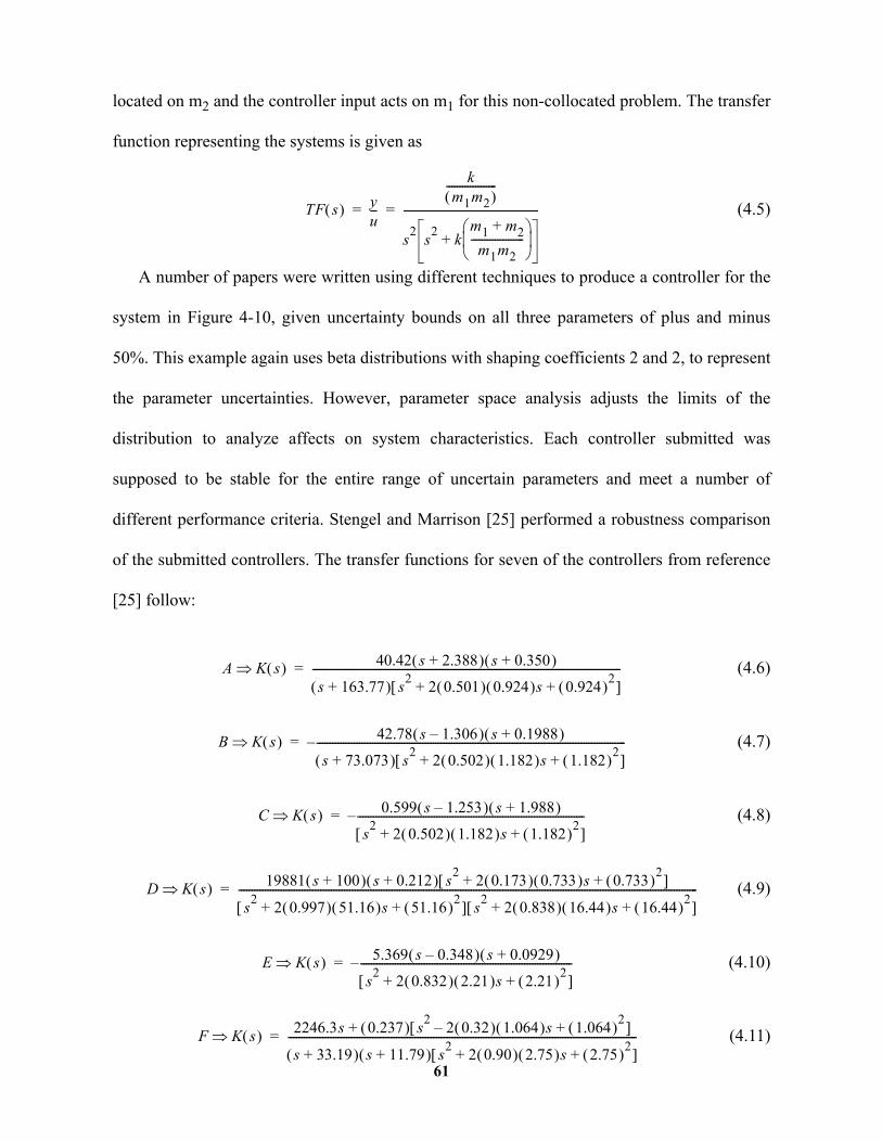
located on m2 and the controller input acts on m1 for this non-collocated problem. The transfer
function representing the systems is given as
(4.5)
A number of papers were written using different techniques to produce a controller for the
system in Figure 4-10, given uncertainty bounds on all three parameters of plus and minus
50%. This example again uses beta distributions with shaping coefficients 2 and 2, to represent
the parameter uncertainties. However, parameter space analysis adjusts the limits of the
distribution to analyze affects on system characteristics. Each controller submitted was
supposed to be stable for the entire range of uncertain parameters and meet a number of
different performance criteria. Stengel and Marrison [25] performed a robustness comparison
of the submitted controllers. The transfer functions for seven of the controllers from reference
[25] follow:
(4.6)
(4.7)
(4.8)
(4.9)
(4.10)
(4.11)
TF s( ) yu---
km1m2( )
-------------------
s2 s2 km1 m2+
m1m2--------------------
+
---------------------------------------------------= =
A K s( )⇒ 40.42 s 2.388+( ) s 0.350+( )
s 163.77+( ) s2 2 0.501( ) 0.924( )s 0.924( )2+ +[ ]---------------------------------------------------------------------------------------------------------------------=
B K s( )⇒ 42.78 s 1.306–( ) s 0.1988+( )
s 73.073+( ) s2 2 0.502( ) 1.182( )s 1.182( )2+ +[ ]---------------------------------------------------------------------------------------------------------------------–=
C K s( )⇒ 0.599 s 1.253–( ) s 1.988+( )
s2 2 0.502( ) 1.182( )s 1.182( )2+ +[ ]--------------------------------------------------------------------------------------–=
D K s( )⇒ 19881 s 100+( ) s 0.212+( ) s2 2 0.173( ) 0.733( )s 0.733( )2+ +[ ]
s2 2 0.997( ) 51.16( )s 51.16( )2+ +[ ] s2 2 0.838( ) 16.44( )s 16.44( )2+ +[ ]------------------------------------------------------------------------------------------------------------------------------------------------------------------------------=
E K s( )⇒ 5.369 s 0.348–( ) s 0.0929+( )
s2 2 0.832( ) 2.21( )s 2.21( )2+ +[ ]--------------------------------------------------------------------------------–=
F K s( )⇒ 2246.3s 0.237( ) s2 2 0.32( ) 1.064( )s– 1.064( )2+[ ]+
s 33.19+( ) s 11.79+( ) s2 2 0.90( ) 2.75( )s 2.75( )2+ +[ ]------------------------------------------------------------------------------------------------------------------------------------=
61

(4.12)
However, the original equations are from the following references [28] A-C, [29] D, [30] E,
and [31] F. The remaining three controllers were unable to be reproduced and give a stable
system. About half of controllers in equations (4.6) through (4.12) have a leading negative sign
to account for inconsistency in negative feedback representation of the original paper.
4.5 Parameter Space Analysis
The probabilistic response plots were developed first, then the hybrid method was reapplied
to explore parameter space analysis. Both performance metric analysis and probability of
instability were found to produce good results, however; the performance metric analysis
exhibited the need for a more problem dependent approach. Most of the parameter space
analysis was performed using beta distributions, a bounded support distribution that has two
shape parameters a and b that prescribe the curvature within the support of the distribution.
4.5.1 Performance Metric Analysis
While many control system performance metrics exist, a few specific performance metrics
were used for the development of the probabilistic performance metric analysis discussed here.
The specific metrics were rise time, peak value, and settling time. There were a few early
hurdles in adapting the hybrid method to performance metric analysis. While the response plot
analysis developed limit state functions directly from response equations, the performance
metrics analyzed in this research required limit state function to be produced based on a
discretely sampled step response. A coarse spacing of time values produced a very nonsmooth
limit state function making the gradient based optimization in MATPA (see section 2.2.3)
H K s( )⇒ 2.13 s 0.145+( ) s 0.98–( ) s 3.43+( )
s2 2 0.82( ) 1.59( )s 1.59( )2+ +[ ] s2 2 0.46( ) 2.24( )s 2.24( )2+ +[ ]------------------------------------------------------------------------------------------------------------------------------------------------------------–=
62
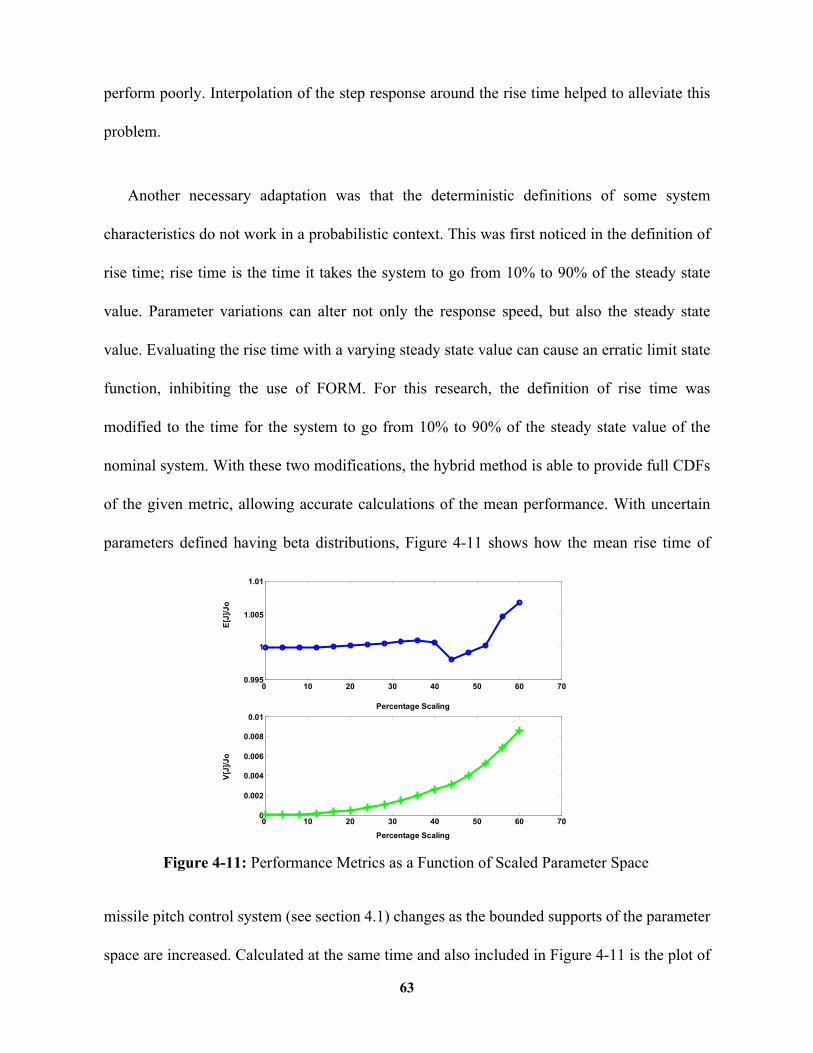
perform poorly. Interpolation of the step response around the rise time helped to alleviate this
problem.
Another necessary adaptation was that the deterministic definitions of some system
characteristics do not work in a probabilistic context. This was first noticed in the definition of
rise time; rise time is the time it takes the system to go from 10% to 90% of the steady state
value. Parameter variations can alter not only the response speed, but also the steady state
value. Evaluating the rise time with a varying steady state value can cause an erratic limit state
function, inhibiting the use of FORM. For this research, the definition of rise time was
modified to the time for the system to go from 10% to 90% of the steady state value of the
nominal system. With these two modifications, the hybrid method is able to provide full CDFs
of the given metric, allowing accurate calculations of the mean performance. With uncertain
parameters defined having beta distributions, Figure 4-11 shows how the mean rise time of
missile pitch control system (see section 4.1) changes as the bounded supports of the parameter
space are increased. Calculated at the same time and also included in Figure 4-11 is the plot of
0 10 20 30 40 50 60 700.995
1
1.005
1.01
Percentage Scaling
E[J]
/Jo
0 10 20 30 40 50 60 700
0.002
0.004
0.006
0.008
0.01
Percentage Scaling
V[J]
/Jo
Figure 4-11: Performance Metrics as a Function of Scaled Parameter Space
63

V[J]/Jo, representing how the variance of the performance metric values increases as the
supports of the parameter space are increased. For the example shown in Figure 4-11 it can be
seen that with uncertain parameters having a range of up to plus and minus 40% of the nominal
values, the expected value of the rise time stays very close to the rise time value of the nominal
system. As the uncertainty is increased the distribution of rise time spreads out, however stays
centralized about the nominal system.
By only changing the limit state function to represent a different performance metric such
as peak value, the exact same analysis method can be used. Each performance metric requires a
different limit state function, and each brought its own unique difficulties. Settling time
provided a few more difficulties than those found working with rise time analysis. With settling
time defined as the time the response last exceeds 2% of the steady state value, uncertainty can
cause large jumps in the settling time value as different oscillations of the response are the last
to exceed 2% deviation from the steady state value. A slight modification to the definition of
settling time is harder to define than it was for rise time. This issue inhibits the use of FORM
reducing the accuracy of the mean calculations. For the settling time analysis the true hybrid
approach only works well when there is enough knowledge of the system step response to
know these jumps in settling time value do not exist. For systems where these issues do not
arise the settling time analysis can be performed in the same manner as the rise time and peak
64

value analysis. Figure 4-12 illustrates the Settling time analysis on the missile pitch control
problem. The expected value analysis in Figure 4-12 shows that with increasing amounts of
uncertainty in this system the expected settling time is slower than the nominal system
This performance metric analysis of the parameter space provides insight into system
performance as the uncertainty of the parameters is allowed to expand. The knowledge of how
desired performance metrics are affected by growing uncertainty bounds can be one additional
tool to help find the most desirable control system, however, cost must also be considered. As
an uncertainty analysis method, the performance metric analysis is less robust than the
probabilistic response plots and requires more knowledge of the system response to ensure an
analysis of the performance metric is achievable. There are cases when the analysis is not valid
such as peak value analysis of an overdamped system, or cases where FORM becomes non-
beneficial such as when gaps in settling time are produced. These added complexities make the
performance metric analysis a much more system specific analysis tool.
0 10 20 30 40 50 60 701
1.05
1.1
1.15
1.2
E[J]
/Jo
0 0.1 0.2 0.3 0.4 0.5 0.6 0.70
0.05
0.1
0.15
0.2
Precentage Scaling
V[J]
/Jo
Precentage Scaling
Figure 4-12: Performance Metrics as a Function of Scaled Parameter Space
65
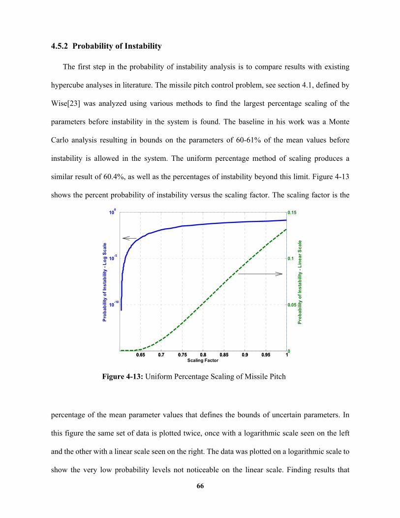
4.5.2 Probability of Instability
The first step in the probability of instability analysis is to compare results with existing
hypercube analyses in literature. The missile pitch control problem, see section 4.1, defined by
Wise[23] was analyzed using various methods to find the largest percentage scaling of the
parameters before instability in the system is found. The baseline in his work was a Monte
Carlo analysis resulting in bounds on the parameters of 60-61% of the mean values before
instability is allowed in the system. The uniform percentage method of scaling produces a
similar result of 60.4%, as well as the percentages of instability beyond this limit. Figure 4-13
shows the percent probability of instability versus the scaling factor. The scaling factor is the
percentage of the mean parameter values that defines the bounds of uncertain parameters. In
this figure the same set of data is plotted twice, once with a logarithmic scale seen on the left
and the other with a linear scale seen on the right. The data was plotted on a logarithmic scale to
show the very low probability levels not noticeable on the linear scale. Finding results that
0.65 0.7 0.75 0.8 0.85 0.9 0.95 1
10-10
10-5
100
Scaling Factor
Prob
abili
ty o
f Ins
tabi
lity
- Log
Sca
le
0.65 0.7 0.75 0.8 0.85 0.9 0.95 10
0.05
0.1
0.15
Prob
abili
ty o
f Ins
tabi
lity
- Lin
ear S
cale
Figure 4-13: Uniform Percentage Scaling of Missile Pitch
66

correlate well with previous research gives confidence that the hybrid method is producing
accurate results.
Analyzing the system with a norm bounded set, or uniform distribution, is beneficial for
comparison to non-probabilistic analysis. The real advantage to the hybrid method is being able
to incorporate distributions such as beta distributions. Most physical parameters do not have a
uniform distribution but one where each value has a different likelihood. The hybrid method
allows the system with different distributions defining the uncertain parameters to be analyzed
and compared. A system analyzed with beta distributions having the same support but different
shape parameters produces different results. Figure 4-14, shows that the point at which stability
is first violated stays similar, however; the rate that probability of instability increases does
change with different parameter distributions. This provides better information about the limits
on the parameter space if a specified probability of instability is acceptable. If a specified
0.65 0.7 0.75 0.8 0.85 0.9 0.95 1
10-10
10-5
100
Scaling Factor
Prob
abili
ty o
f Ins
tabi
lity
- Log
Sca
le
UniformBeta a=2 b=2Beta a=3 b=3
Figure 4-14: Effects of Parameter Distributions on Probability of Instability
67

probability of instability is acceptable, the shape of the distributions representing the uncertain
parameters is important. Assuming a distribution for parameters has consequences if the
uncertain parameters do not closely represent the assumed distribution. If the uncertain
parameters are not closely represented by a uniform distribution, conservative results may be
produced.
Another type of probability analysis compares multiple controllers for a given system.
Using the Benchmark example describe in section 4.4 all controllers are compared in Figure 4-
68

15 and Figure 4-16. This analysis used the uniform percentage scaling method, and the x-axis
20 30 40 50 60 70 80 90 100 0
0.02
0.04
0.06
0.08
0.1
0.12
0.14
0.16
0.18
0.2P
f
HDBEACF
H
D
B
E
A
C
F
Uniform Dialation of Parameter Space (%)
Figure 4-15: Comparison of Benchmark Problem Controllers, Linear Scale
69

values represent the percentage variation of the uncertain variables. That is the x-axis shows the
percentage change in each of the parameters in the system. Controller D is significantly more
robust than the others, while controller A is the least robust. Controller D allows the uncertain
parameters to vary by 60% of the nominal value before any probability of instability, while
controller A will only tolerate a range of parameters within 20% of the nominal values before
any probability of instability. While each controller will accept a different amount of
uncertainty, all have similar rate of growth in probability of instability. Ranked for robustness,
controller D would be the best choice for the system. The results for all the controllers compare
well with the analysis of the controllers in reference [25], which also shows controller D as the
most stable.
20 30 40 50 60 70 80 90 100 10-12
10-10
10-8
10-6
10-4
10-2
100
Pf
HDBEACF
H D
B
E A
C F
Uniform Dialation of Parameter Space (%)
Figure 4-16: Comparison of Benchmark Problem Controllers, Log Scale
70

As described in section 3.6 there are many ways the parameter space hypercube can be
scaled to fit the needs of each problem. Each hypercube scaling technique was used to analyze
the stable parameter space for the missile pitch problem. Table 4-1 shows the nominal values
for the different variables and the delta values each scaling technique provides for the extent of
a stable parameter space. The hypercubes represented by Table 4-1 are the nominal value plus
and minus the delta given in the column of each scaling technique. The uniform percentage
column represents a hypercube with each parameter having 60.4% variation about the nominal
values. Table 4-1 shows that each of the different methods produces a different range of
parameters that leads to instability. The requirements of the problem would determine which
technique provides the best results.
No one scaling method seems to provide the best overall answer, however; each has its own
unique degenerate cases where the method produces poor results. Although unlikely to occur at
the same time, both the method using mppX and the method using the closes point in x-space
have the same type of problem. The problem arises if the closest point on the limit state
Table 4-1: Comparison of Hypercube Scaling Techniques on Missile Pitch Problem
Nominal Values
Uniform Percentage
mppX Closest point in x-space
Gradient of g(x)
Zα=-1.3046 0.788 0.1528 1.3046 1.2383Zδ=-0.2142 0.1293 0.0040 9.3E-07 0.6113Mα=47.711 28.817 9.5976 2.4E-06 0.0197Mδ=-104.83 63.317 76.599 9.7E-07 0.00877
71

function falls on or near an axis of a random variable, see Figure 4-17. When this condition
exists, the hypercube may be disproportionately sensitive in the direction of that parameter.
Though accurate, the parameter space bounds that result may misrepresent how much
parameters may vary before inducing instability. The finite differencing method also has a
drawback. The finite differencing used to find the gradient of g(x) is done at the mean values of
the system, the resultant vector may not point in the direction of the first point of contact
Figure 4-17: Closest Point Hypercube Scaling Problem
x1
x2
72

between the hypercube and the limit state surface. See Figure 4-18 for a representation of this
problem. With this method points were taken along the gradient vector to find when the
hypercube transitions across the limit state function. If the gradient vector doesn’t point to the
first point of contact, techniques must be developed to find the largest hypercube still within the
stable parameter space. This problem can easily be detected if a significant probability of
instability is computed at the starting hypercube. When detected, one method for solving the
issue is to use the MPP found with the FORM calculation and shrink the hypercube until this
point is on the surface of the hypercube. This process may need to be repeated if the scaling of
the hypercube allows for a portion of the limit state function to stay within the hypercube.
However, once that starting hypercube is found with zero probability of instability the analysis
can proceed as usual.
Figure 4-18: Gradient Based Hypercube Scaling Difficulty
x1
x2
∇v
Initial Hypercube
True max stablehypercube
73

Chapter 5
Conclusions
The increasing demand on aerospace control systems requires high performance
characteristics as well as being robust to uncertainties. Individually the two requirements often
oppose each other. A probabilistic approach can produce control systems that both improve
performance as well as improve robustness. A hybrid method for approaching the analysis of
SISO systems with parameter uncertainty in a probabilistic manner has been investigated. A
missile pitch example and spring mass example were used to explore results of the hybrid
method. Incorporating the FORM tools helped provide definition in regions of low probability
without the hundreds of thousands of sample evaluations required with Monte Carlo
techniques.
The developed hybrid method adapted quite well to probabilistic response plots, in both the
frequency and time domain. Applied to a range of the system response, a probabilistic
definition of the specific response plot was easily found. Confidence bounds provide response
limits and indicate the likelihood of the system response exceeding these bounds. These plots
also provide information about areas of the response that are more affected by the parameter
uncertainty. The main difficulty of the hybrid method was the developed extrapolation method
used for selecting FORM locations, although it worked well for most response distributions.
74

Expanding from the probabilistic response plot application, the hybrid method was applied
to parameter space analysis. Due to the nature of many system characteristics the performance
metric analysis required more restructuring of the problem to fit the hybrid method tools. Also
for this type of analysis some prior knowledge is necessary to ensure the performance metric
being analyzed is legitimate over the range of responses seen with increasing uncertainty.
However the performance metric analysis is able to produce useful information on changes in
the uncertainty affected performance metrics. The missile pitch example showed how the
distribution of rise time stays centralized evenly distributed about the nominal parameters.
Results of a similar analysis showed a skewed distribution for settling time where as
uncertainty increased more systems had a settling time later than the nominal system.
The probability of instability analysis performed quite well across a wide range of systems.
While the scaling of the parameter space is arbitrary, four techniques were given and discussed.
Any one of these four techniques, or some other scaling, can be used for most generic systems
when determining the largest parameter uncertainties before a probability of instability exists.
The hybrid method provided information beyond pervious research by mapping the growth in
probability of instability as the amount of uncertainty in the system increased.
The developed hybrid method was found to perform well both for producing probabilistic
response plots and analyzing the effects of varying uncertainty with parameter space analysis.
As a preliminary study this paper has shown many benefits and possibilities of probabilistic
control analysis. This research has shown that the hybrid method for probabilistic analysis
provides previously unavailable information about system responses due to parameter
uncertainty
75

Chapter 6
Future Work
One of the most noticeable areas of future work is moving from the analysis phase to the
design phase. It is mentioned in the introduction, there has been some research performed using
sampling to incorporate probability into control design, however including low probability
analysis tools such as FORM could improve results. Related directly to the hybrid method of
analysis, the addition of SORM could improve results over the use of FORM in some cases.
This research looked at Bode and step responses as two classical analysis tools, however
there are also root locus, Nyquist, and Nichols plots. The hybrid approach to including
probability into the system analysis has not been applied to these analysis methods. The main
challenge with both of these tools is that they display a combined representation of the complex
data. Nyquist plots represent phase versus magnitude while root locus represents the real vs.
imaginary portions of the data. This makes the problem much more difficult because you are
looking at a joint probability distribution that may have high correlation. The difficulty that
prevented the hybrid approach from being applied to these methods was the inability to
separate the joint distribution into independent distributions. The use of FORM inhibited the
ability to accommodate these two analysis tools.
There are many ways for efficiency improvements to be made in the analysis methods,
particularly in the response analysis. Since FORM must be performed separately at each
76

frequency, this analysis could be easily segmented and performed on a distributed computing
system. This would allow for greatly reduced analysis time for a large number of uncertain
parameters, or systems that are more complex. Another option would be to arrange the software
for the hybrid method to perform a slightly more extensive sampling analysis of the overall
system, and then only performing the more detailed analysis at desired locations.
Briefly discussed in section 3.5 was the issue of the inverse MPP problem. In this research,
the standard FORM problem was used to find the probability of failure and extrapolation
techniques were developed attempting to find the desired probability of failure results. The
inverse problem would allow for the probability of failure to be prescribed and the conditions
that produce this probability would be found. Instead of finding the MPP, the distance from the
MPP to the origin is prescribed and the conditions that cause the closest point of the limit state
function to be this prescribed distance from the origin. The inverse problem could allow for a
specified number of FORM computations at prescribed levels.
77

References
[1] Zang, Thomas A., et al., Needs and Opportunities for Uncertainty-Based Multidisciplinary Design Methods for Aerospace Vehicles, NASA/TM-2002-211462, 2002.
[2] Wang, Qian; Stengel, Robert F.; Robust Nonlinear Control of Hypersonic Aircraft, AIAA Journal of Guidance, Control, and Dynamics, Vol. 23, No. 4, Aug. 2000.
[3] Marrison, Christopher I.; Stengel, Robert F.; Design of Robust Control Systems For a Hypersonic Aircraft, AIAA Journal of Guidance, Control, and Dynamics, Vol. 21, No. 1, Feb. 1998.
[4] Bennett, Stuart, A Brief History of Automatic control, IEEE Control Systems 1996.
[5] Nise, Norman S.; Control Systems Engineering, John Wiley & Sons, Inc., 2000.
[6] Balas, Gary J.; Doyle, John C.; et al.; µ-Analysis and Synthesis Toolbox for Use with MATLAB®, MUSYN Inc. and The MathWorks, Inc., 2001.
[7] Wise, Kevin A.; Mears, Barry C., Poolla, Kameshwar; Missile Autopilot Design Using Optimal Control With µ-Synthesis, Proceedings of the American Control Conference,
San Diego, CA. May 1990, pp. 2362-2367.
[8] Toffner-Clausen, Steen; Anderson, Palle, Estimated Frequency Domain Model Uncertainties used in Robust Controller Design - A mu-Approach, Proceedings of the Third IEEE Conference on Control Applications, 1994.
[9] Balas, Gary J.; Doyle, John C., Robustness and Performance Trade-Offs in Control Design for Flexible Structures, IEEE Transactions on Control Systems Technology, Vol. 2, No. 4, Dec. 1994.
[10] Savkin, Andrey V.; Peterson, Ian R.; Ugrinovskii, Vallery A., Robust Control Design Using H-infinity Methods, pp 1-29, Springer-Verlag London, 2000.
[11] Henrion, Didier; Sebek, Micheal; Kucera, Vladimir; Robust pole placement for second-order systems: an LMI approach, 4th IFAC Symposium on Robust Control Design, June 2003.
[12] Shue, Shyh-Pyng; Shi, Peng; Robust Pole Placement of Single Input Uncertain Systems For Control of Aircraft, American Institute of Aeronautics and Astronautics, 1997.
H∞
H∞
78
[13] Stengel, Robert F.; Ray, Laura R.; Stochastic Robustness of Linear Time-Invariant Control Systems, IEEE Transactions on Automatic Control, Vol. 36, No. 1, Jan. 1991.
[14] Hamed, Maged M.; Bendeit, Philip B., Reliability-Based Uncertainty Analysis of Groundwater Contaminant Transport and Remediation, EPA/600/R-99/028, June 1999.
[15] Wyss, Gregory D,; Jorgensen. Kelly H., A User's Guide to LHS: Sandia's Latin Hypercube Sampling Software, Sandia National Laboratories, 1998.
[16] Kalagnanam, Jayant R.; Diwekar Urmila M.; An Efficient Sampling Technique for Off-line Quality Control, Technometrics, Vol. 39, No. 3, Aug. 1997.
[17] Robinson, David G.; A Survey of Probabilistic Methods Used in Reliability, Risk and Uncertainty Analysis: Analytical Techniques I, Sandia National Laboratories, SAND98-1189, June 1998.
[18] Rackwitz, Rudiger, Reliability Analysis - Past Present and Future. 8th ASCE Specialty Conference on Probabilistic Mechanics and Structural Reliability, PCM2000-RRR, July 2000.
[19] Giunta, Anthony A.; Wojtkiewicz Jr., S. F.; Eldred, M. S.; Overview of Modern Design of Experiments Methods for Computational Simulations, American Institute of Aeronautics and Astronautics, 2003.
[20] Robinson, D.; Atcitty, C.; Comparison of Quasi- and Pseudo-Monte Carlo Sampling for Reliability and Uncertainty Analysis, American Institute of Aeronautics and Astronautics, 1999.
[21] Papoulis, Athanasios; Probability, Random Variables, And Stochastic Processes, McGraw Hill, Inc., 1991.
[22] Wise, Kevin A.; Nguyen, Tam; Optimal Disturbance Rejection in Missile Autopilot Design Using Projective Controls, IEEE, October 1992.
[23] Wise, Kevin A.; Kundur, Sridhar; Missile Autopilot Robustness to Real and Complex Uncertainties Using A Parameter Space Robustness Test, AIAA Guidance, Navigation and Control Conference, August 1993.
[24] Phillips, Charles L.;Harbor, Royce D.; Feedback Control Systems, Prentice Hall, 2000.
[25] Stengel, Robert F.; Marrison, Christopher I.; Robustness of solutions to a benchmark Control Problem, AIAA Journal of Guidance, Control, and Dynamics, Vol. 15, No. 5, Oct. 1992.
[26] Wie, B.; Bernstein, D.S.; A benchmark Problem for Robust Control Design, Proceedings of the 1990 American Control Conference, May 1990, pp. 961-962.
79

[27] Yaz, Engin. Deterministic and Stochastic Robustness Measures for Discrete Systems, IEEE Transactions on Automatic Control, Vol. 33, No. 10, Oct. 1988.
[28] Byrns Jr, Edward V.;Calise, Anthony J.; Fixed Order Dynamic Compensation for the H2/ Benchmark Problem, Proceedings of the 1990 American Controls Conference, May
1990.
[29] Chiang, R. Y.; Safonov, M.G.; Robust Control Synthesis for an Underdamped, Non-colocated Spring-Mass System, Proceedings of the 1990 American Controls Conference, May 1990.
[30] Ly, Uy-Loi; Robust Control Design Using Nonlinear Constrained Optimization, Proceedings of the 1990 American Controls Conference, May 1990.
[31] Collins, Jr., E .G.; Bernstein, D. S.; Robust Control Design for a Benchmark Problem Using a Structured Covariance Approach, Proceedings of the 1990 American Controls Conference, May 1990.
H∞
H∞
80

REPORT DOCUMENTATION PAGE Form ApprovedOMB No. 0704-0188
2. REPORT TYPE
Technical Memorandum 4. TITLE AND SUBTITLE
Probabilistic Parameter Uncertainty Analysis of Single Input Single Output Control Systems
5a. CONTRACT NUMBER
6. AUTHOR(S)
Smith, Brett A.; Kenny, Sean P.; and Crespo, Luis G.
7. PERFORMING ORGANIZATION NAME(S) AND ADDRESS(ES)
NASA Langley Research Center George Washington University Hampton, VA 23681-2199 303 Butler Farm Rd. Suite 106A Hampton, VA 23666
9. SPONSORING/MONITORING AGENCY NAME(S) AND ADDRESS(ES)
National Aeronautics and Space AdministrationWashington, DC 20546-0001
8. PERFORMING ORGANIZATION REPORT NUMBER
L-18389
10. SPONSOR/MONITOR'S ACRONYM(S)
NASA
13. SUPPLEMENTARY NOTESBrett: George Washington University; Kenny: Langley Research Center; Grespo: National Institute of Aerospace.An electronic version can be found at http://ntrs.nasa.gov
12. DISTRIBUTION/AVAILABILITY STATEMENTUnclassified - UnlimitedSubject Category 08Availability: NASA CASI (301) 621-0390
19a. NAME OF RESPONSIBLE PERSON
STI Help Desk (email: [email protected])
14. ABSTRACT
The current standards for handling uncertainty in control systems use interval bounds for definition of the uncertain parameters. This approach gives no information about the likelihood of system performance, but simply gives the response bounds. When used in design, current methods of m-analysis and can lead to overly conservative controller design. With these methods, worst case conditions are weighted equally with the most likely conditions. This research explores a unique approach for probabilistic analysis of control systems. Current reliability methods are examined showing the strong areas of each in handling probability. A hybrid method is developed using these reliability tools for efficiently propagating probabilistic uncertainty through classical control analysis problems. The method developed is applied to classical response analysis as well as analysis methods that explore the effects of the uncertain parameters on stability and performance metrics. The benefits of using this hybrid approach for calculating the mean and variance of responses cumulative distribution functions are shown. Results of the probabilistic analysis of a missile pitch control system, and a non-collocated mass spring system, show the added information provided by this hybrid analysis.
15. SUBJECT TERMS
Probability; Control Analysis; Probabilistic Control; Hammersley; First Order Reliability Methods
18. NUMBER OF PAGES
93
19b. TELEPHONE NUMBER (Include area code)
(301) 621-0390
a. REPORT
U
c. THIS PAGE
U
b. ABSTRACT
U
17. LIMITATION OF ABSTRACT
UU
Prescribed by ANSI Std. Z39.18Standard Form 298 (Rev. 8-98)
3. DATES COVERED (From - To)
5b. GRANT NUMBER
5c. PROGRAM ELEMENT NUMBER
5d. PROJECT NUMBER
5e. TASK NUMBER
5f. WORK UNIT NUMBER
23-762-45-G7
11. SPONSOR/MONITOR'S REPORT NUMBER(S)
NASA/TM-2005-213280
16. SECURITY CLASSIFICATION OF:
The public reporting burden for this collection of information is estimated to average 1 hour per response, including the time for reviewing instructions, searching existing data sources, gathering and maintaining the data needed, and completing and reviewing the collection of information. Send comments regarding this burden estimate or any other aspect of this collection of information, including suggestions for reducing this burden, to Department of Defense, Washington Headquarters Services, Directorate for Information Operations and Reports (0704-0188), 1215 Jefferson Davis Highway, Suite 1204, Arlington, VA 22202-4302. Respondents should be aware that notwithstanding any other provision of law, no person shall be subject to any penalty for failing to comply with a collection of information if it does not display a currently valid OMB control number.PLEASE DO NOT RETURN YOUR FORM TO THE ABOVE ADDRESS.
1. REPORT DATE (DD-MM-YYYY)
03 - 200501-