Computing F

Epipolar geometry: basic equation0Fxx'T

separate known from unknown

0'''''' 333231232221131211 fyfxffyyfyxfyfxyfxxfx

0,,,,,,,,1,,,',',',',',' T333231232221131211 fffffffffyxyyyxyxyxxx

(data) (unknowns)(linear)

0Af

0f1''''''

1'''''' 111111111111

nnnnnnnnnnnn yxyyyxyxyxxx

yxyyyxyxyxxx

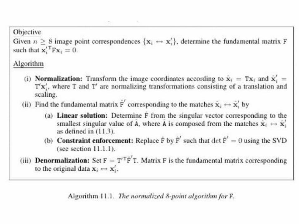
If A has rank 8 soln unique up to a scale factorFor noisy data, rank of A might be larger than 8 least squares solnMinimize || Af || subject to ||f|| = 1 singular vector for smallest sing. value of AThis is called “8 point” algorithm

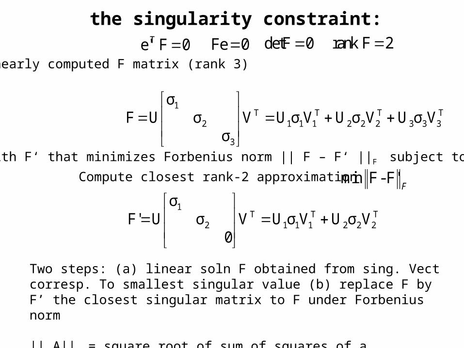
the singularity constraint: 0Fe'T 0Fe 0detF 2Frank

T333

T222

T111

T

3

2

1

VσUVσUVσUVσ

σσ

UF

SVD from linearly computed F matrix (rank 3)

Replace F with F‘ that minimizes Forbenius norm || F – F‘ ||F subject to det(F‘) = 0

T222

T111

T2

1

VσUVσUV0

σσ

UF'

FF'-FminCompute closest rank-2 approximation

Two steps: (a) linear soln F obtained from sing. Vect corresp. To smallest singular value (b) replace F by F’ the closest singular matrix to F under Forbenius norm

|| A||F = square root of sum of squares of ai,j

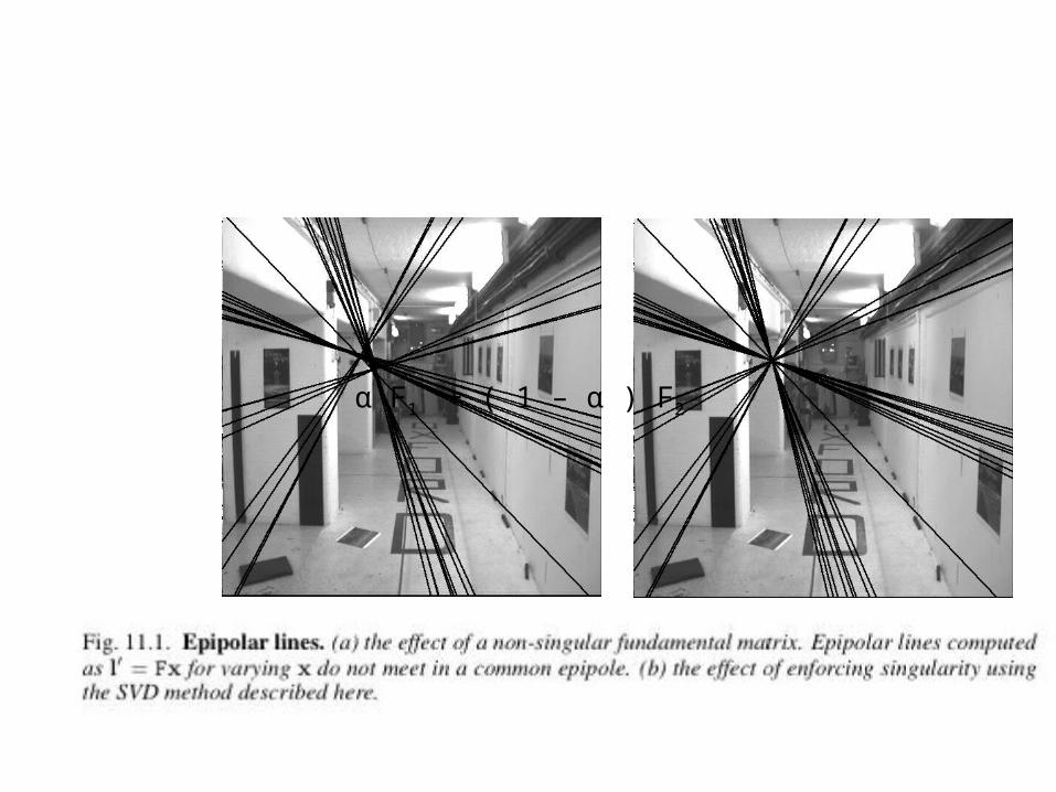
α F1 + ( 1 – α ) F2

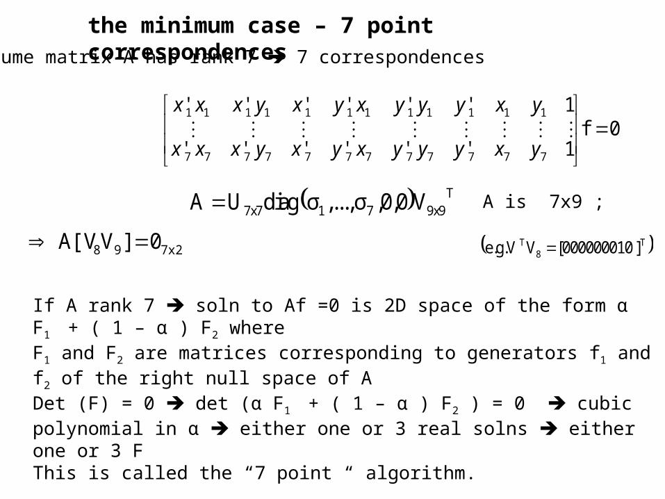
the minimum case – 7 point correspondences

0f1''''''

1''''''

777777777777

111111111111

yxyyyxyxyxxx

yxyyyxyxyxxx

T9x9717x7 V0,0,σ,...,σdiagUA

7x298 0]VA[V T8

T ] 000000010[Ve.g.V

Assume matrix A has rank 7 7 correspondences

A is 7x9 ;

If A rank 7 soln to Af =0 is 2D space of the form α F1 + ( 1 – α ) F2 whereF1 and F2 are matrices corresponding to generators f1 and f2 of the right null space of ADet (F) = 0 det (α F1 + ( 1 – α ) F2 ) = 0 cubic polynomial in α either one or 3 real solns either one or 3 FThis is called the “7 point “ algorithm.

0

1´´´´´´

1´´´´´´

1´´´´´´

33

32

31

23

22

21

13

12

11

222222222222

111111111111

f

f

f

f

f

f

f

f

f

yxyyyyxxxyxx

yxyyyyxxxyxx

yxyyyyxxxyxx

nnnnnnnnnnnn

~10000 ~10000 ~10000 ~10000~100 ~100 1~100 ~100

!Orders of magnitude differenceBetween column of data matrix least-squares yields poor results

the NOT normalized 8-point algorithm

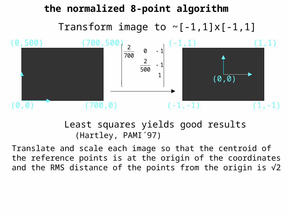
Transform image to ~[-1,1]x[-1,1]

(0,0)

(700,500)

(700,0)

(0,500)

(1,-1)

(0,0)

(1,1)(-1,1)

(-1,-1)

1

1500

2

10700

2

Least squares yields good results (Hartley, PAMI´97)

the normalized 8-point algorithm

Translate and scale each image so that the centroid of the reference points is at the origin of the coordinates and the RMS distance of the points from the origin is √2

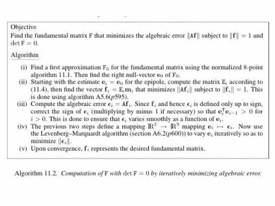
algebraic minimization

Find F‘ with rank 2 directly, i.e. Find singular matrix F‘ that minimizes || A F‘|| subject to ||F‘|| = 1

• Arbitrary singular matrix F can be written as F = M [e]x where M is nonsingular and [e]x is any skew symmetrix matrix

• For now, assume e is known

• F = M [e]x f = Em where f and m are vectors corresponding to F and M matrices and

• Minimize || A E m || subject to || Em || = 1

• Apply Algorithm A.5.6 from Hartley and Zisserman

Geometric distance

Gold standard

Sampson error

Symmetric epipolar distance

Gold standard

Maximum Likelihood Estimation

i

iiii dd 22 'x̂,x'x̂,x

(= least-squares for Gaussian noise)

0x̂F'x̂ subject to T

iXt],|[MP'0],|[IP Parameterize:

Initialize: normalized 8-point, (P,P‘) from F, reconstruct Xi

iiii XP''x̂,PXx̂

Minimize cost using Levenberg-Marquardt(preferably sparse LM, see book)

(overparametrized)

xi and x’I measured correspondence; and true correspondence

Find F to minimize

i'x̂ix̂

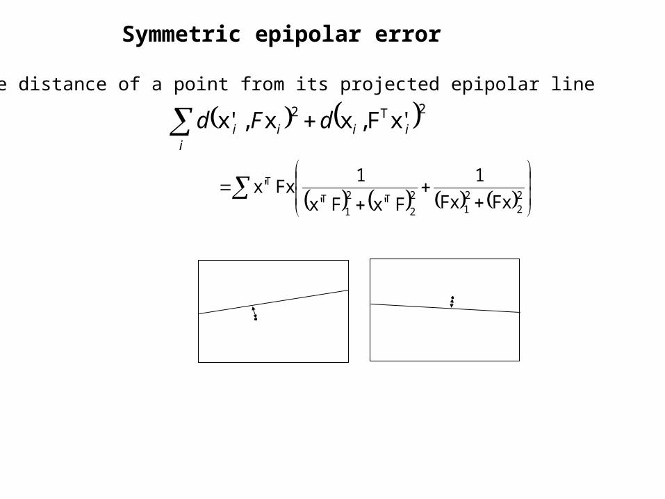
Symmetric epipolar error

2

221

2

2T2

1T

T

FxFx

1

Fx'Fx'

1Fxx'

i

iiii dFd2T2 x'F,xx,x'

Minimize distance of a point from its projected epipolar line

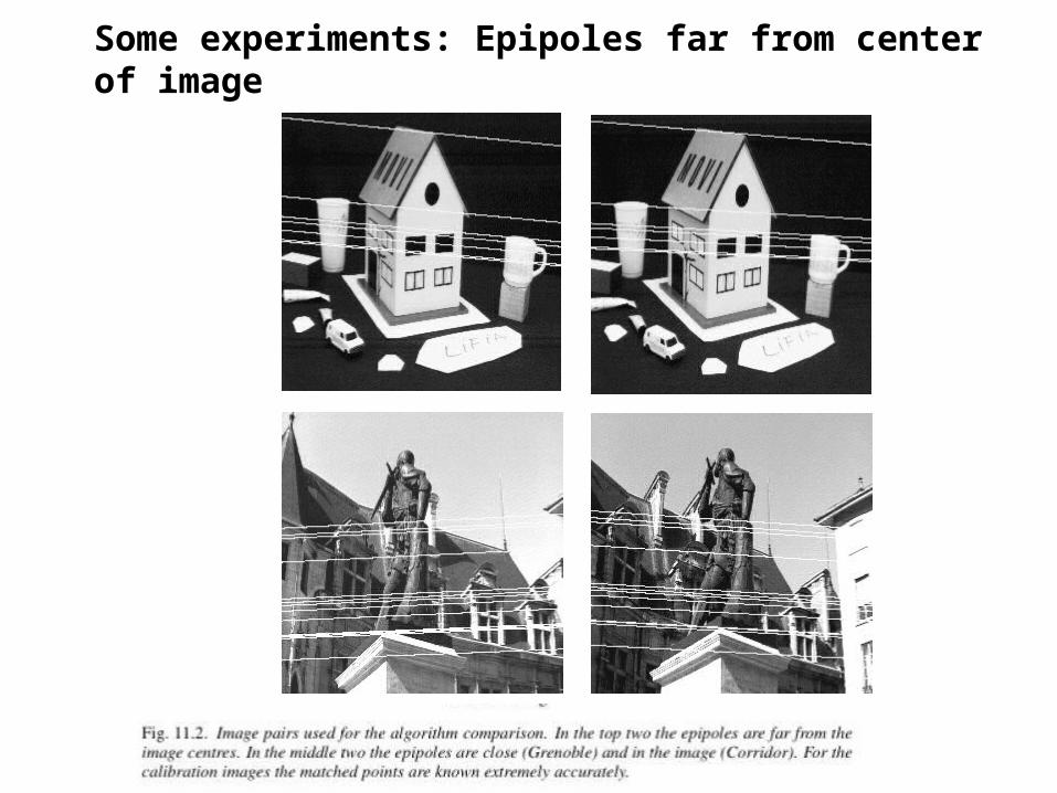
Some experiments: Epipoles far from center of image

Some experiments:

Epipoles in the image

Epipoles closeto image

Some experiments:

Matched points known extremely accurately

Algorithm comparison

• Normalized 8 point (alg. 11.1)• Min. Algebraic error while imposing singularlity (Alg.

11.2)• Gold standard algorithm (Alg. 11.3)• N = total number of correspondences• Choose n out of N points randomly 100 times• Find average residual error vs. n

• Squared distance between a point’s epipolar line and the other image averaged over all N

• This is not directly minimized by any of the 3 algorithms

NdFdi

iiii /)x'F,xx,x'(2T2

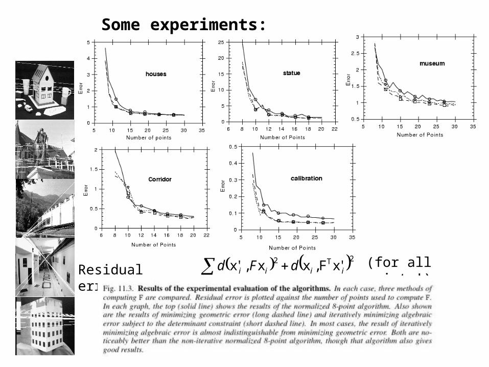
Some experiments:

i

iiii dFd2T2 x'F,xx,x' (for all points!)Residual error:

Recommendations:

1. Do not use unnormalized algorithms

2. Quick and easy to implement: 8-point normalized (alg. 11.1)

3. Better: enforce rank-2 constraint during minimization (alg. 11.2)

4. Best: Maximum Likelihood Estimation (alg. 11.3) (minimal parameterization, sparse implementation)

Automatic computation of F

(i) Interest points(ii) Putative correspondences(iii) RANSAC (iv) Non-linear re-estimation of F(v) Guided matching(repeat (iv) and (v) until stable)

• Extract feature points to relate images

• Required properties:• Well-defined

(i.e. neigboring points should all be different)

• Stable across views(i.e. same 3D point should be extracted as feature for neighboring viewpoints)

Feature points

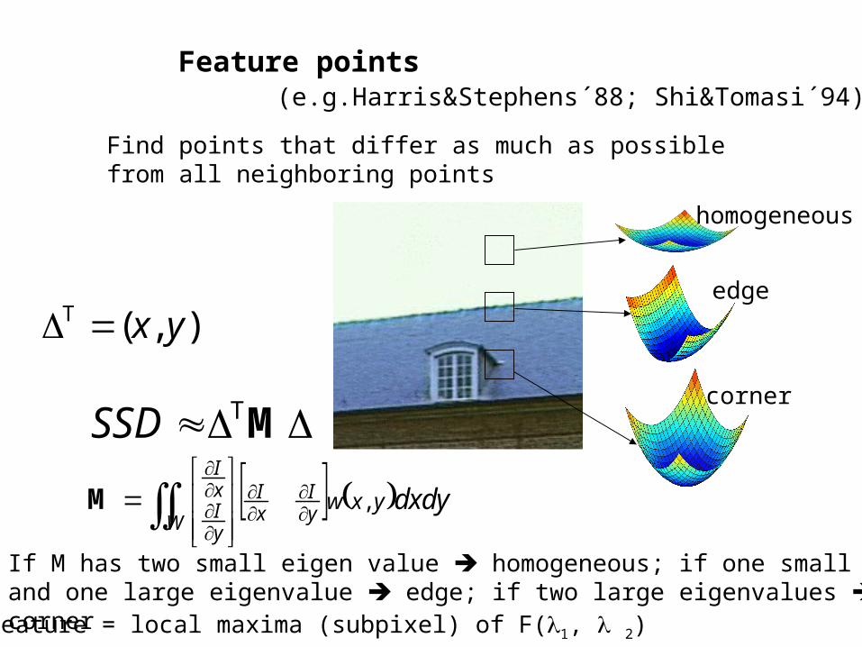
homogeneous

edge

corner

dxdyyxwyI

xI

W yIxI

,

M

If M has two small eigen value homogeneous; if one small and one large eigenvalue edge; if two large eigenvalues corner

(e.g.Harris&Stephens´88; Shi&Tomasi´94)

MTSSD

Find points that differ as much as possible from all neighboring points

Feature = local maxima (subpixel) of F(1, 2)

Feature points

),( yxT

Select strongest features (e.g. 1000/image)

Feature points

Evaluate NCC for all features withsimilar coordinates

Keep mutual best matchesKeep mutual best matches

Still many wrong matches!Still many wrong matches!

10101010 ,,´´, e.g. hhww yyxxyx

?

Feature matching

0.96 -0.40 -0.16 -0.39 0.19

-0.05 0.75 -0.47 0.51 0.72

-0.18 -0.39 0.73 0.15 -0.75

-0.27 0.49 0.16 0.79 0.21

0.08 0.50 -0.45 0.28 0.99

1 5

24

3

1 5

24

3

Gives satisfying results for small image motions

Feature example

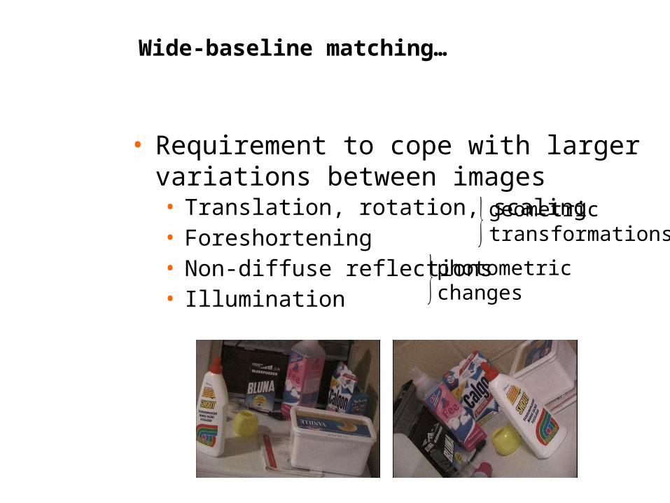
• Requirement to cope with larger variations between images• Translation, rotation, scaling• Foreshortening• Non-diffuse reflections• Illumination

geometric transformations

photometric changes

Wide-baseline matching…

Wide baseline matching for two different region types

(Tuytelaars and Van Gool BMVC 2000)

Wide-baseline matching…

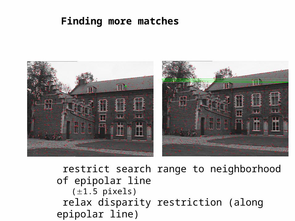
restrict search range to neighborhood of epipolar line (1.5 pixels)

relax disparity restriction (along epipolar line)

Finding more matches

Step 1. Extract featuresStep 2. Compute a set of potential matchesStep 3. do

Step 3.1 select minimal sample (i.e. 7 matches)

Step 3.2 compute solution(s) for F

Step 3.3 determine inliers

until (#inliers,#samples)<95%

samples#7)1(1

matches#inliers#

#inliers 90%

80%

70% 60%

50%

#samples

5 13 35 106 382

Step 4. Compute F based on all inliersStep 5. Look for additional matchesStep 6. Refine F based on all correct matches

(generate hypothesis)

(verify hypothesis)

RANSAC

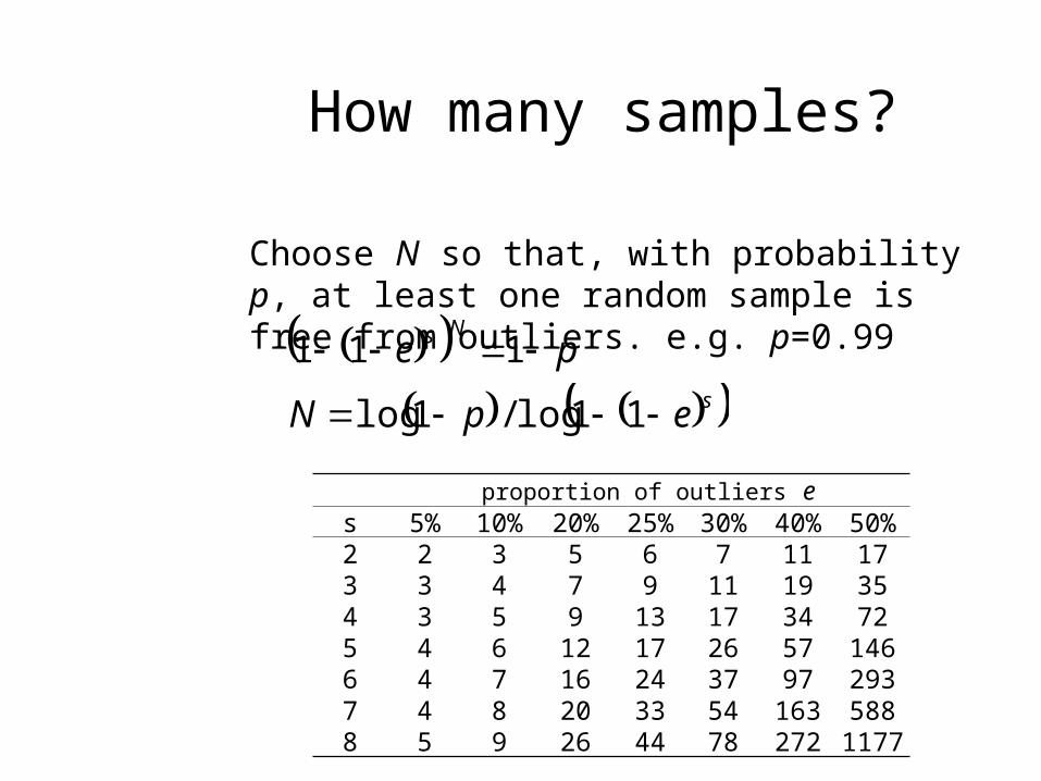
How many samples?

Choose N so that, with probability p, at least one random sample is free from outliers. e.g. p=0.99

sepN 11log/1log

peNs 111

proportion of outliers es 5% 10% 20% 25% 30% 40% 50%2 2 3 5 6 7 11 173 3 4 7 9 11 19 354 3 5 9 13 17 34 725 4 6 12 17 26 57 1466 4 7 16 24 37 97 2937 4 8 20 33 54 163 5888 5 9 26 44 78 272 117

7

• Absence of sufficient features (no texture)• Repeated structure ambiguity

(Schaffalitzky and Zisserman, BMVC‘98)

• Robust matcher also finds Robust matcher also finds support for wrong hypothesissupport for wrong hypothesis• solution: detect repetition solution: detect repetition

More problems:

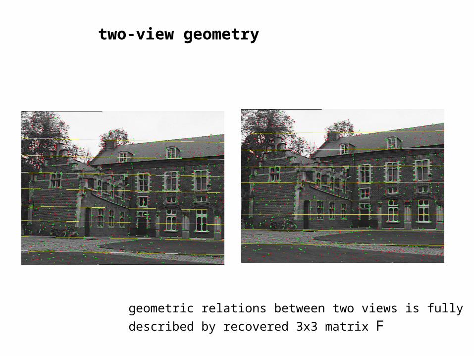
geometric relations between two views is fully

described by recovered 3x3 matrix F

two-view geometry

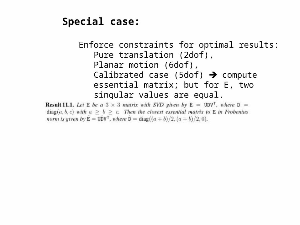
Special case:

Enforce constraints for optimal results:Pure translation (2dof), Planar motion (6dof), Calibrated case (5dof) compute essential matrix; but for E, two singular values are equal.