Principles of Programming in Econometrics
220
PPEctr Principles of Programming in Econometrics Introduction, structure, and advanced programming techniques Charles S. Bos VU University Amsterdam Tinbergen Institute [email protected] August 2019 – Version Python Lecture slides Compilation: August 23, 2019 1/203
Transcript of Principles of Programming in Econometrics

PPEctr
Principles of Programming in EconometricsIntroduction, structure, and advanced programming techniques
Charles S. Bos
VU University AmsterdamTinbergen Institute
August 2019 – Version PythonLecture slides
Compilation: August 23, 2019
1/203

PPEctr
Target
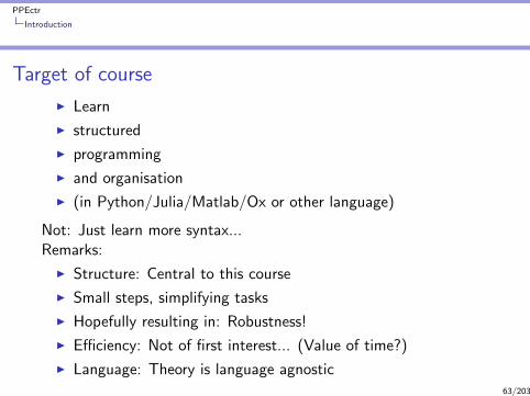
Target of course
I Learn
I structured
I programming
I and organisation
I (in Python/Julia/Matlab/Ox or other language)
Not only: Learn more syntax... (mostly today)Remarks:
I Structure: Central to this course
I Small steps, simplifying tasks
I Hopefully resulting in: Robustness!
I Efficiency: Not of first interest... (Value of time?)
I Language: Theory is language agnostic2/203

PPEctr
Target
Target of course II
... Or move from
3/203

PPEctr
Target
Target of course II
... Or move from
to(Maybe discuss at end of first day?...)
3/203
PPEctr
Syntax: Start
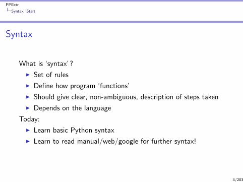
Syntax
What is ‘syntax’?
I Set of rules
I Define how program ‘functions’
I Should give clear, non-ambiguous, description of steps taken
I Depends on the language
Today:
I Learn basic Python syntax
I Learn to read manual/web/google for further syntax!
4/203
PPEctr
Syntax: Start
Syntax II
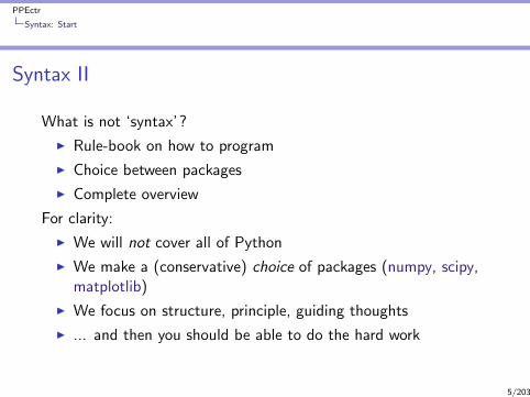
What is not ‘syntax’?
I Rule-book on how to program
I Choice between packages
I Complete overview
For clarity:
I We will not cover all of Python
I We make a (conservative) choice of packages (numpy, scipy,matplotlib)
I We focus on structure, principle, guiding thoughts
I ... and then you should be able to do the hard work
5/203

PPEctr
Program
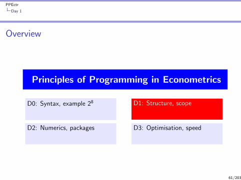
Overview
Principles of Programming in Econometrics
D0: Syntax, example 28 D1: Structure, scope
D2: Numerics, packages D3: Optimisation, speed
6/203
PPEctr
Program
Day 0: Syntax
9.30 Introduction
Example: 28
Elements
Main concepts
Closing thoughts
Revisit E0
13.30 Practical (at VU, main building)I Checking variables, types, conversion and functionsI Implementing Backsubstitution
7/203

PPEctr
Program
Day 1: Structure
9.30 IntroductionI Programming in theoryI Science, data, hypothesis, model, estimation
Structure & Blocks (Droste)
Further concepts ofI Data/Variables/TypesI FunctionsI Scope, globals
13.30 PracticalI Regression: Simulate dataI Regression: Estimate model
8/203

PPEctr
Program
Day 2: Numerics and flow
9.30 Numbers and representation
I Steps, flow and structure
I Floating point numbers
I Practical Do’s and Don’ts
I Packages
I Graphics
13.30 PracticalI Cleaning OLS programI LoopsI Bootstrap OLS estimationI Handling data: Inflation
9/203
PPEctr
Program
Day 3: Optimisation
9.30 Optimization (minimize)I Idea behind optimizationI Gauss-Newton/Newton-RaphsonI Stream/order of function calls
I Standard deviations
I Restrictions
I Speed
13.30 PracticalI Regression: Maximize likelihoodI GARCH-M: Intro and likelihood
10/203

PPEctr
Program
Evaluation
I No old-fashioned exam
I Range of exercises, to try out during course
I Short voluntary final exercise (see VU Canvas, TBA). If youhand it in, you may receive some comments/hints onprogramming style.
Main message: Work for your own interest, later courses will besimpler if you make good use of this course...
11/203

PPEctr
Day 0
Overview
Principles of Programming in Econometrics
D0: Syntax, example 28 D1: Structure, scope
D2: Numerics, packages D3: Optimisation, speed
12/203

PPEctr
Day 0
Day 0: Syntax
9.30 Introduction
Example: 28
Elements
Main concepts
Closing thoughts
Revisit E0
13.30 Practical (at VU, main building)I Checking variables, types, conversion and functionsI Implementing Backsubstitution
13/203

PPEctr
Example: 28
Programming by example
Let’s start simple
I Example: What is 28?
I Goal: Simple situation, program to solve it
I Broad concepts, details follow
14/203
PPEctr
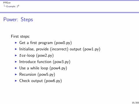
Example: 28
Power: Steps
First steps:
I Get a first program (pow0.py)
I Initialise, provide (incorrect) output (pow1.py)
I for-loop (pow2.py)
I Introduce function (pow3.py)
I Use a while loop (pow4.py)
I Recursion (pow5.py)
I Check output (pow6.py)
15/203
PPEctr
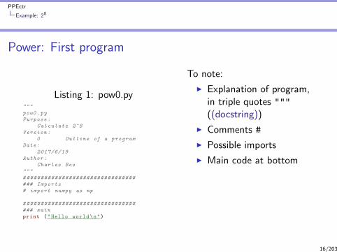
Example: 28
Power: First program
Listing 1: pow0.py"""
pow0.py
Purpose:
Calculate 2^8
Version:
0 Outline of a program
Date:
2017/6/19
Author:
Charles Bos
"""
# ###############################
### Imports
# import numpy as np
# ###############################
### main
print ("Hello world\n")
To note:
I Explanation of program,in triple quotes """
((docstring))
I Comments #
I Possible imports
I Main code at bottom
16/203

PPEctr
Example: 28
Power: Initialise
Listing 2: pow1.py# Magic numbers
dBase= 2
iC= 8
# Initialisation
dRes= 1
# Estimation
# Not done yet ...
# Output
print ("The result of ", dBase , "^", iC,
"= ", dRes , "\n")
To note:
I Each line is a command
I Distinction between‘magics’, ‘initialisation’,‘estimation’ and ‘output’
I Function print(a, b,
c) is used
17/203
PPEctr
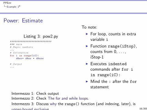
Example: 28
Power: Estimate
Listing 3: pow2.py# ##########################
### main
# Magic numbers
...
# Estimation
for i in range(iC):
dRes= dRes * dBase
# Output
...
To note:
I For loop, counts in extravariable i
I Function range(iStop),counts from 0, . . . ,iStop-1
I Executes indented
commands after for i
in range(iC):
I Mind the : after the for
statement
Intermezzo 1: Check outputIntermezzo 2: Check The for and while loops.
Intermezzo 3: Discuss why the range() function (and indexing, later), is
upper-bound exclusive. 18/203

PPEctr
Example: 28
Power: Functions
Listing 4: pow3.pydef Pow(dBase , iPow):
"""
Purpose:
Calculate dBase^iPow
Inputs:
dBase double , base
iPow integer , power
Return value:
dRes double , dBase^iPow
"""
dRes= 1
for i in range(iPow):
# print ("i= ", i)
dRes= dRes * dBase
return dRes
### Main
dRes= Pow(dBase , iC)
To note:
I Function has owndocstring
I Function defines twoarguments dBase, iPow
I Function indents one tabforward
I Uses local dRes, i
I returns the result
I And dRes= Pow(dBase,
iC) catches the result;cf. dRes= 256.
I Allows to re-use functions for multiple purposesI Could also be called as dRes= Pow(4, 7)I Here, only one output
19/203

PPEctr
Example: 28
Power: While
Listing 5: pow3.pydRes= 1
for i in range(iC):
dRes= dRes*dBase
Listing 6: pow4.pydRes= 1
i= 0
while (i < iPow):
dRes= dRes*dBase
i+= 1
To note:I The for i in range(iter) loop corresponds to a while
loopI Look at the order: First init, then check, then action, then
increment, and check again.I The for-loop is slightly simpler, as beforehand the number of
iterations is fixed.I A loop command can be a compound command, multiple
commands all indented equally.20/203

PPEctr
Example: 28
Power: Recursion
Listing 7: pow5.pydef Pow_Recursion(dBase , iPow):
# print ("In Pow_Recursive , with iPow= ", iPow)
if (iPow == 0):
return 1
return dBase * Pow_Recursion(dBase , iPow -1)
To note:
I 28 ≡ 2× 27
I 20 ≡ 1
I Use this in a recursion
I New: If statement
Intermezzo: Check Python manual on if statement, or a simplerWiki on the same topic.Q: What is wrong, or maybe just non-robust in this code?
A: Rather use if (iPow <= 0), do not continue for non-positiveiPow!
21/203

PPEctr
Example: 28
Power: Recursion
Listing 8: pow5.pydef Pow_Recursion(dBase , iPow):
# print ("In Pow_Recursive , with iPow= ", iPow)
if (iPow == 0):
return 1
return dBase * Pow_Recursion(dBase , iPow -1)
To note:
I 28 ≡ 2× 27
I 20 ≡ 1
I Use this in a recursion
I New: If statement
Intermezzo: Check Python manual on if statement, or a simplerWiki on the same topic.Q: What is wrong, or maybe just non-robust in this code?A: Rather use if (iPow <= 0), do not continue for non-positiveiPow!
21/203

PPEctr
Example: 28
Power: Check outcome
Always, (always...!) check your outcome
Listing 9: pow6.pyimport math
...
# Output
print ("The result of ", dBase , "^", iC, "= ")
print (" - Using Pow (): ", Pow(dBase , iC))
print (" - Using Pow_Recursion (): ", Pow_Recursion(dBase , iC))
print (" - Using **: ", dBase ** iC)
print (" - Using math.pow: ", math.pow(dBase , iC))
Listing 10: outputThe result of 2 ^ 8 =
- Using Pow (): 256
- Using Pow_Recursion (): 256
- Using **: 256
- Using math.pow: 256.0
22/203
PPEctr
Example: 28
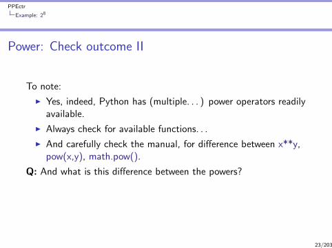
Power: Check outcome II
To note:
I Yes, indeed, Python has (multiple. . . ) power operators readilyavailable.
I Always check for available functions. . .
I And carefully check the manual, for difference between x**y,pow(x,y), math.pow().
Q: And what is this difference between the powers?
A: According to the manual, math.pow() transforms first tofloats, then computes. The others leave integers intact.
23/203

PPEctr
Example: 28
Power: Check outcome II
To note:
I Yes, indeed, Python has (multiple. . . ) power operators readilyavailable.
I Always check for available functions. . .
I And carefully check the manual, for difference between x**y,pow(x,y), math.pow().
Q: And what is this difference between the powers?A: According to the manual, math.pow() transforms first tofloats, then computes. The others leave integers intact.
23/203

PPEctr
Elements
Elements to considerI Comments: # (until end of line)
I Docstring: """ Docstring """
I import statements: At front of each code fileI Spacing: Important for routines/loops/conditional statementsI Variables, types and naming (subset):
boolean bX=True
scalar integer iN= 20
scalar double/float dC= 4.5
string sName=’Beta1’
list lX= [1, 2, 3], lY= [’Hello’, 2, True]
tuple tX= (1, 2, 3)
vector vX= np.array([1, 2, 3, 4])
matrix mX= np.array([[1, 2.5], [3, 4]])
function fnFunc = print
24/203
PPEctr
Elements
Elements: Comments
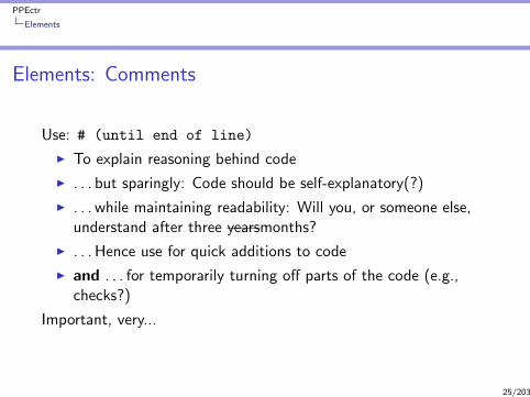
Use: # (until end of line)
I To explain reasoning behind code
I . . . but sparingly: Code should be self-explanatory(?)
I . . . while maintaining readability: Will you, or someone else,understand after three yearsmonths?
I . . . Hence use for quick additions to code
I and . . . for temporarily turning off parts of the code (e.g.,checks?)
Important, very...
25/203

PPEctr
Elements
Elements: DocstringsUse:
I To explain the functions/modules you writeI Either single-line
(‘"""Return the iPow’th power of dBase."""),I or multi-line, after function defintion:
def Pow_Recursion(dBase, iPow):"""Purpose:
Calculate dBase^iPow through recursion
Inputs:dBase double, baseiPow integer, power
Return value:dRes double, dBase^iPow
"""
I . . . and at start of module, explainingname/purpose/version/date/author
Important, indeed...26/203
PPEctr
Elements
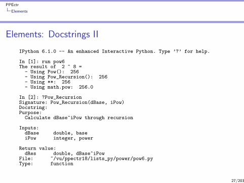
Elements: Docstrings II
IPython 6.1.0 -- An enhanced Interactive Python. Type ’?’ for help.
In [1]: run pow6The result of 2 ^ 8 =
- Using Pow(): 256- Using Pow_Recursion(): 256- Using **: 256- Using math.pow: 256.0
In [2]: ?Pow_RecursionSignature: Pow_Recursion(dBase, iPow)Docstring:Purpose:
Calculate dBase^iPow through recursion
Inputs:dBase double, baseiPow integer, power
Return value:dRes double, dBase^iPow
File: ~/vu/ppectr18/lists_py/power/pow6.pyType: function
27/203
PPEctr
Elements
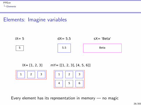
Elements: Imagine variables
iX= 5
5
dX= 5.5
5.5
sX= 'Beta'
Beta
lX= [1, 2, 3]
1 2 3
mY= [[1, 2, 3], [4, 5, 6]]
1 2 3
4 5 6
Every element has its representation in memory — no magic28/203
PPEctr
Elements
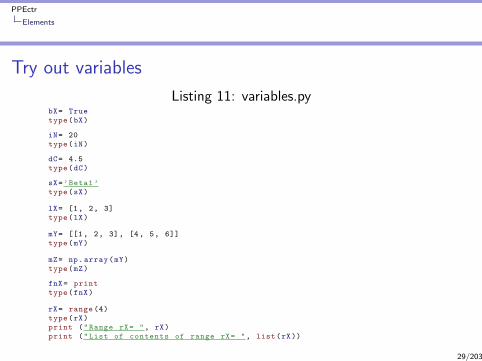
Try out variables
Listing 11: variables.pybX= Truetype(bX)
iN= 20type(iN)
dC= 4.5type(dC)
sX=’Beta1’type(sX)
lX= [1, 2, 3]type(lX)
mY= [[1, 2, 3], [4, 5, 6]]type(mY)
mZ= np.array(mY)type(mZ)
fnX= printtype(fnX)
rX= range (4)type(rX)print ("Range rX= ", rX)print ("List of contents of range rX= ", list(rX))
29/203
PPEctr
Elements
Hungarian notation
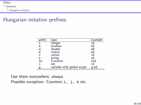
Hungarian notation prefixes
prefix type examplei integer iXb boolean bXd double dXm matrix mXv vector vXs string sXfn Function fnXl list lXg variable with global scope g mX
Use them everywhere, always.Possible exception: Counters i, j, k etc.
30/203

PPEctr
Elements
Hungarian notation
Hungarian 2
Python does not force Hungarian notation. Why would you?
I Forces you to think: What should each object be?
I Improves readability of code
I Helps (tremendously) in debugging
Drawbacks:
I Python recognizes many different types; in ‘EOR/QRM/PhD’,not all are useful to track
I Hungarian notation best used for ‘intention’: vector vX for1-dimensional list or array or a n × 1 or 1× n matrix, matrixmX for 2-dimensional list/array
31/203
PPEctr
Elements
Hungarian notation
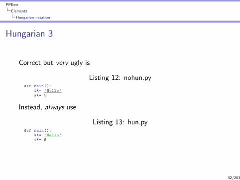
Hungarian 3
Correct but very ugly is
Listing 12: nohun.pydef main ():
iX= ’Hello’
sX= 5
Instead, always use
Listing 13: hun.pydef main ():
sX= ’Hello’
iX= 5
32/203
PPEctr
Recap
Recap
But let us recap the first lessons, and extend the knowledge...
33/203

PPEctr
Recap of main concepts
Functions
All work in functionsAll work is done in functions (or at least, that’s what we’ll do!)
Listing 14: recap1.pydef main ():
dX= 5.5
dX2= dX ** 2
print ("The square of ", dX , " is ", dX2)
# ##########################################################
### start main
if __name__ == "__main__":
main()
Note:
I This function main() takes no argumentsI . . . but Python only executes the first line outside a functionI . . . which is an if statement, calling main()
I . . . only if we call this routine as a separate program (allows usto import files later)
34/203

PPEctr
Recap of main concepts
Functions
Quiz-time: Main
Listing 15: recap quiz.pydef main ():
print ("Hello world")
# ##########################################################
### start main
print ("This is an orphan statement")
if __name__ == "__main__":
main()
Q1 What is the output of this program?
Q2 Would anything change if the line starting with if is skipped?
Q3 And why does one use the conditional statement?
Answer: Deep Python philosophy. But follow the custom...
35/203

PPEctr
Recap of main concepts
Functions
Quiz-time: Main
Listing 16: recap quiz.pydef main ():
print ("Hello world")
# ##########################################################
### start main
print ("This is an orphan statement")
if __name__ == "__main__":
main()
Q1 What is the output of this program?
Q2 Would anything change if the line starting with if is skipped?
Q3 And why does one use the conditional statement?
Answer: Deep Python philosophy. But follow the custom...
35/203

PPEctr
Recap of main concepts
Functions
Squaring and printingUse other functions to do your work for you
Listing 17: recap2.pyimport math
def printsquare(dIn):
dOut= math.pow(dIn , 2)
print ("The square of ", dIn , " is ", dOut)
def main ():
dX= 5.5
printsquare(dX)
printsquare (6.3)
Here, printsquare does not give a return value, only screenoutput.printsquare takes in one argument, with a value locally calleddIn. Can either be a true variable (dX), a constant (6.3), or eventhe outcome of a calculation (dX-5).Note the usage of import math for the math.pow() function.
36/203

PPEctr
Recap of main concepts
Return statement
Return
Use return a to give one value back to the calling function (ase.g. the math.pow() function also gives a value back).
Listing 18: recap return.pydef createones(iR, iC):
mX= np.ones((iR , iC)) # Use numpy , handing over Tuple (iR , iC)
return mX
def main ():
iR= 2 # Magic numbers
iC= 5
mX= createones(iR, iC) # Estimation , catch output of createones
print ("Matrix mX=\n", mX) # Output
Alternative: See below, altering pre-defined mutable (= matrix) argument
37/203
PPEctr
Recap of main concepts
Return statement
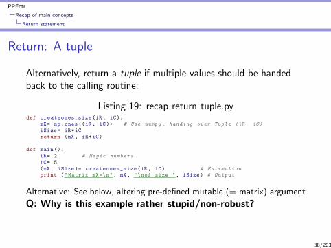
Return: A tuple
Alternatively, return a tuple if multiple values should be handedback to the calling routine:
Listing 19: recap return tuple.pydef createones_size(iR, iC):
mX= np.ones((iR , iC)) # Use numpy , handing over Tuple (iR , iC)
iSize= iR*iC
return (mX, iR*iC)
def main ():
iR= 2 # Magic numbers
iC= 5
(mX , iSize)= createones_size(iR, iC) # Estimation
print ("Matrix mX=\n", mX, "\nof size ", iSize) # Output
Alternative: See below, altering pre-defined mutable (= matrix) argument
Q: Why is this example rather stupid/non-robust?
A: Rather use mX.size, no space for errors
38/203

PPEctr
Recap of main concepts
Return statement
Return: A tuple
Alternatively, return a tuple if multiple values should be handedback to the calling routine:
Listing 20: recap return tuple.pydef createones_size(iR, iC):
mX= np.ones((iR , iC)) # Use numpy , handing over Tuple (iR , iC)
iSize= iR*iC
return (mX, iR*iC)
def main ():
iR= 2 # Magic numbers
iC= 5
(mX , iSize)= createones_size(iR, iC) # Estimation
print ("Matrix mX=\n", mX, "\nof size ", iSize) # Output
Alternative: See below, altering pre-defined mutable (= matrix) argument
Q: Why is this example rather stupid/non-robust?A: Rather use mX.size, no space for errors
38/203

PPEctr
Recap of main concepts
Indexing and matrices
IndexingA matrix is a NumPy array of multiple doubles, a string consists ofmultiple characters, a list of multiple elements. Get to thoseelements by using indices (starting at 0):
Listing 21: recap3.pydef index(mA, sB, lC):
print ("Element [0,1] of\n", mA, "\nis %g" % mA[0 ,1])
print ("Elements [0:5] of ’%s’ are ’%s’" % (sB, sB [0:5]))
print ("Element [4] of ’%s’ is letter ’%s’" % (sB, sB[4]))
print ("Element [1] of\n", lC, "\nis ’%s’" % lC[1])
# ##########################################################
### main
def main ():
mX= np.random.randn(2, 3) # Some random numbers
sY= ’Hello world’ # A string
lZ= (mX, sY, 6.3) # A list of items
index(mX, sY, lZ)
Warnings:I Indexing starts at [0] (as in C, Java, Julia, Ox etc, fine)I Selecting a range indicates [start:end+1]... Extremely
dangerous, if you use other languages... And ugly,according to Prof E.W. Dijkstra
39/203
PPEctr
Recap of main concepts
Indexing and matrices
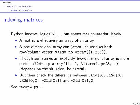
Indexing matrices
Python indexes ‘logically’. . . , but sometimes counterintuitively.
I A matrix is effectively an array of an array
I A one-dimensional array can (often) be used as bothrow/column vector, vX1d= np.array([1,2,3]).
I Though sometimes an explicitly two-dimensional array is moreuseful, vX2d= np.array([1, 2, 3]).reshape(3, 1)
(depends on the situation, be careful)
I But then check the difference between vX1d[0], vX2d[0],vX2d[0,0], vX2d[0:1] and vX2d[0:1,0]
See recap4.py. . .
40/203

PPEctr
Recap of main concepts
Indexing and matrices
Indexing matrices II
Listing 22: recap4.pyimport numpy as np
# ##########################################################
### main
def main ():
vX= np.array([1, 2, 3]). reshape(3, 1) # A column vector
print ("vX=\n", vX)
print ("Note how vX is a lists -of -lists , cast to a two -dimensional array\n")
print ("vX[0]= ", vX[0], "(a one -dimensional array)")
print ("vX[0,0]= ", vX[0,0], "(a scalar)")
print ("vX [0:1]= ", vX[0:1], "(a 1 x 1 matrix)")
# ##########################################################
### start main
if __name__ == "__main__":
main()
41/203

PPEctr
Recap of main concepts
Indexing and matrices
Stepwise Indexing
An index may also take a step:
Listing 23: recap4b.pyimport numpy as np
# ##########################################################
### main
def main ():
vX= np.random.randn (10)
print ("Full vX:\n", vX)
print ("Every second element :\n", vX [::2])
print ("Every second element , starting at second :\n", vX [1::2])
Convenient for selecting subsets!
42/203

PPEctr
Recap of main concepts
Indexing and matrices
Boolean Indexing
One can also index using (a vector of) booleans, to select only therows/columns/elements where the boolean is True:
Listing 24: recap4c.pyimport numpy as np
# ##########################################################
### main
def main ():
vX= np.random.randn(10, 1)
vI= vX >= 0
print (pd.DataFrame(np.append(vX , vI, axis= 1), columns =["X", "I"]))
vXP= vX[vI]
print ("Non -negative elements :\n", vXP)
print ("(Careful with resulting type/size!)")
Convenient for selecting subsets!
43/203

PPEctr
Recap of main concepts
Indexing and matrices
MatricesA matrix:
I . . . is the work-horse of most econometric work (data, linearalgebra, likelihoods and derivatives etc)
I . . . is not natively included in Python
I . . . hence we’ll take the numpy array instead
I (Note: We’ll choose not to use the numpy matrix)
I Matrices tend to be two-dimensional
I . . . hence we’ll often force our matrices/vectors into suchshape:
vX= [1, 2, 3] # A one - dimensional list
vX= np.array(vX) # ... transformed into a one - dimensional array
vX= vX.reshape(3, 1) # ... and made into a two - dimensional matrix
vX= vX.reshape(-1, 1) # ... same thing , Python checks row size
I Important: Check your matrices, make sure you distinguishmatrix/one-dimensional array/scalar!
44/203
PPEctr
Recap of main concepts
Indexing and matrices
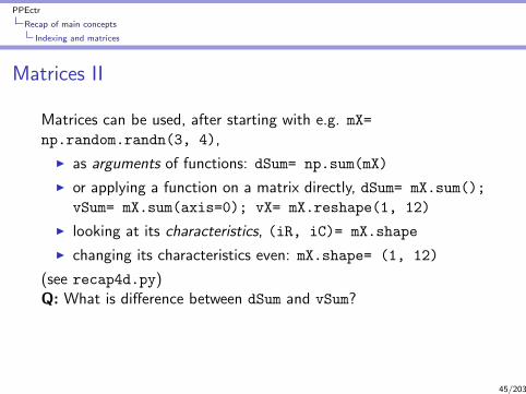
Matrices II
Matrices can be used, after starting with e.g. mX=
np.random.randn(3, 4),
I as arguments of functions: dSum= np.sum(mX)
I or applying a function on a matrix directly, dSum= mX.sum();
vSum= mX.sum(axis=0); vX= mX.reshape(1, 12)
I looking at its characteristics, (iR, iC)= mX.shape
I changing its characteristics even: mX.shape= (1, 12)
(see recap4d.py)Q: What is difference between dSum and vSum?
Hint: Always, always keep track of what your matrix is, and checkyourself...
45/203
PPEctr
Recap of main concepts
Indexing and matrices
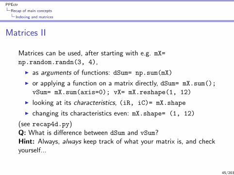
Matrices II
Matrices can be used, after starting with e.g. mX=
np.random.randn(3, 4),
I as arguments of functions: dSum= np.sum(mX)
I or applying a function on a matrix directly, dSum= mX.sum();
vSum= mX.sum(axis=0); vX= mX.reshape(1, 12)
I looking at its characteristics, (iR, iC)= mX.shape
I changing its characteristics even: mX.shape= (1, 12)
(see recap4d.py)Q: What is difference between dSum and vSum?Hint: Always, always keep track of what your matrix is, and checkyourself...
45/203
PPEctr
Recap of main concepts
Indexing and matrices
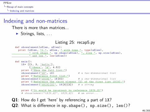
Indexing and non-matricesThere is more than matrices...
I Strings, lists, . . .
Listing 25: recap5.pydef showelement(sElem , aElem ):
print (sElem , "= ", aElem , " with type ", type(aElem),
" with shape ", np.shape(aElem), ", size ", np.size(aElem),
" and len ", len(aElem ))
def main ():
lX= [[1, 2, ’hello’],
[’there’, "A", 4.5]]
print ("Show the full list:")
showelement("lX", lX) # a two - dimensional list
print ("Reference first list:")
showelement("lX[0]", lX[0]) # a one - dimensional list
print ("Reference the third element [2] of the first list lX[0]:")
showelement("lX [0][2]", lX [0][2]) # a string
print ("It would be incorrect to reference lX[0,2]")
# showelement ("lX[0,2]", lX [0 ,2]) # an error ...
Q1: How do I get ‘here’ by referencing a part of lX?Q2: What is difference in np.shape(), np.size(), len()?
46/203
PPEctr
Recap of main concepts
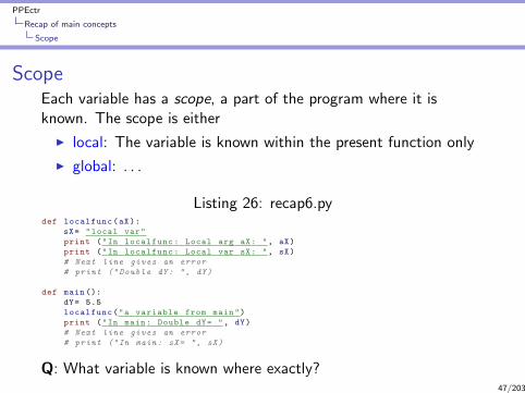
Scope
ScopeEach variable has a scope, a part of the program where it isknown. The scope is either
I local: The variable is known within the present function only
I global: . . .
Listing 26: recap6.pydef localfunc(aX):
sX= "local var"
print ("In localfunc: Local arg aX: ", aX)
print ("In localfunc: Local var sX: ", sX)
# Next line gives an error
# print (" Double dY: ", dY)
def main ():
dY= 5.5
localfunc("a variable from main")
print ("In main: Double dY= ", dY)
# Next line gives an error
# print ("In main: sX= ", sX)
Q: What variable is known where exactly?47/203

PPEctr
Recap of main concepts
Scope
Scope II
Each function (including main)
I can create/use at will new local variables
I can receive through arguments variables from other functions
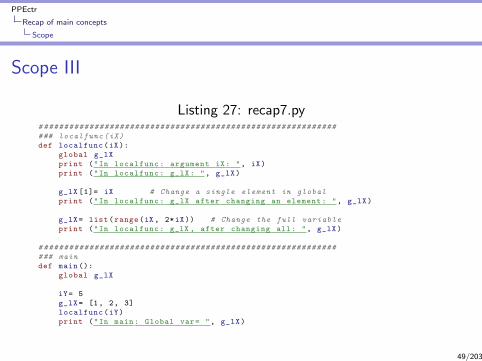
Additionally, each function can
I share a global variable
I where the global variable shall be prefixed by g , as in g mX
I . . . where the variable is declared global within a function,before its use, see recap7.py
48/203
PPEctr
Recap of main concepts
Scope
Scope III
Listing 27: recap7.py# ##########################################################
### localfunc (iX)
def localfunc(iX):
global g_lX
print ("In localfunc: argument iX: ", iX)
print ("In localfunc: g_lX: ", g_lX)
g_lX [1]= iX # Change a single element in global
print ("In localfunc: g_lX after changing an element: ", g_lX)
g_lX= list(range(iX, 2*iX)) # Change the full variable
print ("In localfunc: g_lX , after changing all: ", g_lX)
# ##########################################################
### main
def main ():
global g_lX
iY= 5
g_lX= [1, 2, 3]
localfunc(iY)
print ("In main: Global var= ", g_lX)
49/203

PPEctr
Recap of main concepts
Scope
Scope IV
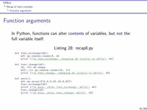
Each function (including main)
I can create/use at will new local variables
I can receive through arguments variables from other functions
I can use global variables (but please forget them...)
Additionally, each function can
I change part of the mutable variable (list/array/matrix) ...Then the variable does not change, only part of the contents
[Example: See recap8.py below]
50/203
PPEctr
Recap of main concepts
Function arguments
Function arguments
In Python, functions can alter contents of variables, but not thefull variable itself:
Listing 28: recap8.pydef func_nochange(mX):
mX= np.random.randn(3, 4)
print ("In func_nochange , changing mX locally to mX=\n", mX)
def func_change(mX):
iR, iC= mX.shape
mX[:,:]= np.random.randn(iR, iC)
print ("In func_change , changing mX locally to mX=\n", mX)
def main ():
mX= np.array ([[1.0 ,2 ,3] ,[4 ,5 ,6]])
func_nochange(mX)
print ("In main , after func_nochange: mX=\n", mX)
func_change(mX)
print ("In main , after func_change: mX=\n", mX)
51/203
PPEctr
Recap of main concepts
Function arguments
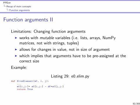
Function arguments II
Limitations: Changing function arguments
I works with mutable variables (i.e. lists, arrays, NumPymatrices, not with strings, tuples)
I allows for changes in value, not in size of argument
I which implies that arguments have to be pre-assigned at thecorrect size
Example:
Listing 29: e0 elim.pydef ElimElement(mC , i, j):
...
mC[i,j:]= mC[i,j:] - dF*mC[j,j:]
return True
52/203

PPEctr
Closing thoughts
Closing thoughts
Almost enough for today...Missing are:
I Operators for ndarraysI Precise definition of compound statements
I if-elif-elseI whileI for
I Corresponding concepts in Matlab
I Many, many details. . .
During this course,
Open the Python/NumPy documentation
and learn to find your way
53/203

PPEctr
Installation
Base installation of PythonMany ways. . . Here:
I MiniConda (https://conda.io/miniconda.html): Thisinstalls the base Python 3.7, with minimal fuss. On Windows,add the Miniconda3 and Miniconda3\scripts directories toyour path.
I At Conda command prompt (= terminal on OSX/Linux),install packages spyder IPython, Matplotlib, NumPy, SciPy,HDF5, Pandas and StatsModels through
conda install ipython matplotlib numpy scipy hdf5 \
pandas statsmodels
I Once in a while, update it all from Conda command prompt,using
conda update --all
conda clean --all54/203
PPEctr
Installation
Full installation of Python
Alternatively, use a full installation of anaconda:
I AnaConda (https://www.anaconda.com/download/): Thisinstalls the base Python 3.7+packages+Spyder, with minimalfuss.
I At Conda command prompt (= terminal on OSX/Linux),update occasionally, using
conda update --all
conda clean --all
55/203
PPEctr
Installation
Editor/IDEFor editing/running programs, several options again:
I Whatever editor of choice, run from command line (go ahead)I Spyder: Install (if needed) through
conda install spyder
I Atom: Install from https://atom.io with packagesHydrogen, Autocomple-python, and add
conda install jupyter
I IPython: Install (if needed) through
conda install ipython
(You’ll probably see me switching; I use Atom for all editing of Python, R, Ox, LATEX,
but sometimes prefer Spyder, IPython for quick testing)
56/203
PPEctr
Installation
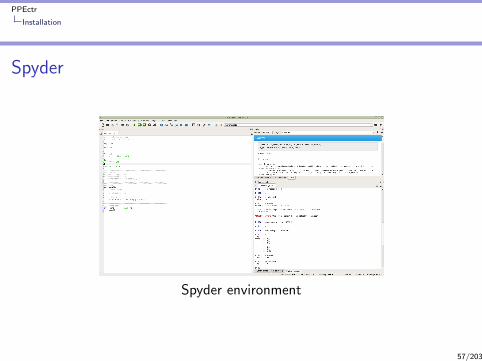
Spyder
Spyder environment
57/203
PPEctr
Installation
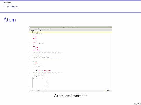
Atom
Atom environment
58/203

PPEctr
Installation
IPython
IPython environment
59/203

PPEctr
Afternoon Day 0
Afternoon session
Practical atVU UniversityMain building, HG 0B08 (EOR/QRM), 0B16 (TI-MPhil)13.30-16.00h
Topics:
I Checking variables and functions
I Implementing Backsubstitution
I Secret message (if time permits, should be easy)
60/203
PPEctr
Day 1
Overview
Principles of Programming in Econometrics
D0: Syntax, example 28 D1: Structure, scope
D2: Numerics, packages D3: Optimisation, speed
61/203

PPEctr
Day 1
Day 1: Structure
9.30 IntroductionI Programming in theoryI Science, data, hypothesis, model, estimation
Structure & Blocks (Droste)
Further concepts ofI Data/Variables/TypesI FunctionsI Scope, globals
13.30 PracticalI Regression: Simulate dataI Regression: Estimate model
62/203
PPEctr
Introduction
Target of course
I Learn
I structured
I programming
I and organisation
I (in Python/Julia/Matlab/Ox or other language)
Not: Just learn more syntax...Remarks:
I Structure: Central to this course
I Small steps, simplifying tasks
I Hopefully resulting in: Robustness!
I Efficiency: Not of first interest... (Value of time?)
I Language: Theory is language agnostic63/203

PPEctr
Introduction
What? Why?Wrong answer:
For the fun of it
A correct answer
To get to the results we need, in a fashion that iscontrollable, where we are free to implement the newestand greatest, and where we can be ‘reasonably’ sure ofthe answers
Data
HypothesisE= f(m)
ModelE= m c2
EstimationE²= m² (c²)2
0
1
1
1
1
1
1
10
1
1
0
0
1
1
Pro
gra
mm
ing
Science
64/203
PPEctr
Introduction
Aims and objectives
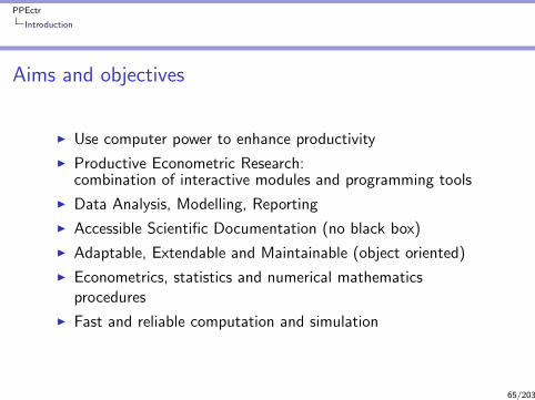
I Use computer power to enhance productivity
I Productive Econometric Research:combination of interactive modules and programming tools
I Data Analysis, Modelling, Reporting
I Accessible Scientific Documentation (no black box)
I Adaptable, Extendable and Maintainable (object oriented)
I Econometrics, statistics and numerical mathematicsprocedures
I Fast and reliable computation and simulation
65/203

PPEctr
Introduction
Options for programming
GU
I
CL
I
Pro
gram
Sp
eed
Qu
anE
con
CommentEViews + - - ± + Black box, TS
Stata ± + - - - Less programmingMatlab + + + + ± Expensive, other audience
Gauss ± ± + ± + ‘Ugly’ code, unstableS+/R ± + + - ± Very common, many packages
Ox + ± + + + Quick, links to C, ectricsPython + + + + ± Neat syntax, common
Julia + + + ++ + General/flexible/difficult, quickC(++)/Fortran - - + ++ - Very quick, difficult
Here: Use Ox Matlab Python as environment, apply theoryelsewhere
66/203

PPEctr
Introduction
History
There was once. . .Apple II, CPU 6502, 1Mhz, 48kB of memory. . .Now: More possibilities, also computationally:
Timings for OLS (30 observations, 4 regressors):2017 I5-7Y54 1.2Ghz 64b 1.047.000†/sec
2014 I5-4460S 2.9Ghz 64b 1.100.000†/sec
2012 Xeon E5-2690 2.9Ghz 64b 950.000†/sec
2009 Xeon X5550 2.67Ghz 64b 670.000†/sec
2008 Xeon 2.8Ghz OSX 392.000†/sec
2006 AMD3500+ 64b 320.000†/sec
2004 PM-1200 147.000†/sec
2001 PIII-1000 104.000†/sec2000 PIII-500 60.000/sec1996 PPro200 30.000/sec1993 P5-90 6.000/sec1989 386/387 300/sec1981 86/87 (est.) 30/sec
Increase:≈ × 1000 in 15 years≈ × 10000 in 25 years.
Note: For further speed increase, use multi-cpu.
67/203

PPEctr
Introduction
Speed increase — but keep thinking
x ∼ NIG(α, β, δ, µ) P(X < x) =
∫ x
0f (z)dz = F (x) xq = F−1(q)
S(q) =x1−q + xq − 2x 1
2
x1−q − xqKL(q) =
x 1−q2
+ x q2− 2x 1
4
x 1−q2− x q
2
KR(q) = ...
-0.15
-0.1
-0.05
0
0.05
0.1
0.15
0 0.05 0.1 0.15 0.2 0.25 0.3 0.35 0.4 0.45 0.5
S x qσSE(S)
-0.4
-0.2
0
0.2
0.4
0.6
0.8
1
1.2
0 0.05 0.1 0.15 0.2 0.25 0.3 0.35 0.4 0.45 0.5
KL x lσKLE(KL) x l
-0.2
-0.1
0
0.1
0.2
0.3
0.4
0.5
0.6
0.7
0.5 0.55 0.6 0.65 0.7 0.75 0.8 0.85 0.9 0.95 1
KR x rσKR x rE(KR) x r
Direct calculation of graph: > 40 min
Pre-calc quantiles (=memoization): 5 sec
68/203

PPEctr
Introduction
Speed increase — but keep thinking
x ∼ NIG(α, β, δ, µ) P(X < x) =
∫ x
0f (z)dz = F (x) xq = F−1(q)
S(q) =x1−q + xq − 2x 1
2
x1−q − xqKL(q) =
x 1−q2
+ x q2− 2x 1
4
x 1−q2− x q
2
KR(q) = ...
-0.15
-0.1
-0.05
0
0.05
0.1
0.15
0 0.05 0.1 0.15 0.2 0.25 0.3 0.35 0.4 0.45 0.5
S x qσSE(S)
-0.4
-0.2
0
0.2
0.4
0.6
0.8
1
1.2
0 0.05 0.1 0.15 0.2 0.25 0.3 0.35 0.4 0.45 0.5
KL x lσKLE(KL) x l
-0.2
-0.1
0
0.1
0.2
0.3
0.4
0.5
0.6
0.7
0.5 0.55 0.6 0.65 0.7 0.75 0.8 0.85 0.9 0.95 1
KR x rσKR x rE(KR) x r
Direct calculation of graph: > 40 minPre-calc quantiles (=memoization): 5 sec
68/203

PPEctr
Programming in theory
Programming in Theory
Plan ahead
I Research question: What do I want to know?
I Data: What inputs do I have?
I Output: What kind of output do I expect/need?I Modelling:
I What is the structure of the problem?I Can I write it down in equations?
I Estimation: What procedure for estimation is needed (OLS,ML, simulated ML, GMM, nonlinear optimisation, Bayesiansimulation, etc)?
69/203
PPEctr
Programming in theory
Blocks & names
Closer to practice
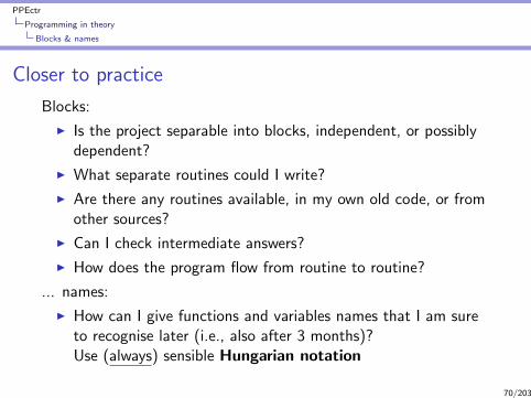
Blocks:
I Is the project separable into blocks, independent, or possiblydependent?
I What separate routines could I write?
I Are there any routines available, in my own old code, or fromother sources?
I Can I check intermediate answers?
I How does the program flow from routine to routine?
... names:
I How can I give functions and variables names that I am sureto recognise later (i.e., also after 3 months)?Use (always) sensible Hungarian notation
70/203

PPEctr
Programming in theory
Input/output
Even closer to practice
Define, on paper, for each routine/step/function:
I What inputs it has (shape, size, type, meaning), exactly
I What the outputs are (shape, size, type, meaning), alsoexactly...
I What the purpose is...
Also for your main program:
I Inputs can be magic numbers, (name of) data file, but alsospecification of model
I Outputs could be screen output, file with cleansed data,estimation results etc. etc.
71/203
PPEctr
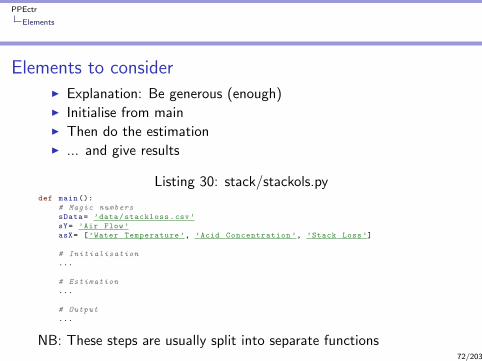
Elements
Elements to considerI Explanation: Be generous (enough)I Initialise from mainI Then do the estimationI ... and give results
Listing 30: stack/stackols.pydef main ():
# Magic numbers
sData= ’data/stackloss.csv’
sY= ’Air Flow’
asX= [’Water Temperature ’, ’Acid Concentration ’, ’Stack Loss’]
# Initialisation
...
# Estimation
...
# Output
...
NB: These steps are usually split into separate functions72/203

PPEctr
Droste
The ‘Droste effect’
I The program performs a certain function
I The main function is split in three (here)
I Each subtask is again a certain function that has to beperformed
Apply the Droste effect:
I Think in terms of functions
I Analyse each function to split it
I Write in smallest building blocks73/203
PPEctr
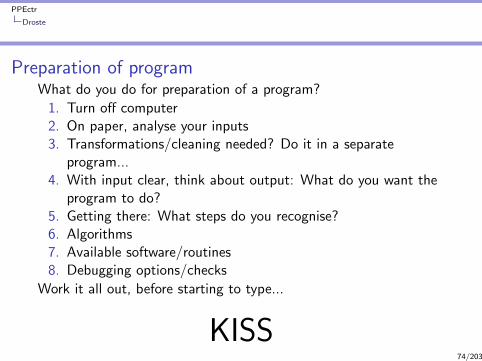
Droste
Preparation of programWhat do you do for preparation of a program?
1. Turn off computer2. On paper, analyse your inputs3. Transformations/cleaning needed? Do it in a separate
program...4. With input clear, think about output: What do you want the
program to do?5. Getting there: What steps do you recognise?6. Algorithms7. Available software/routines8. Debugging options/checks
Work it all out, before starting to type...
KISS74/203

PPEctr
KISS
KISSKeep it simple, stupid
Implications:
I Simple functions, doing one thing only
I Short functions (one-two screenfuls)
I With commenting on top
I Clear variable names (but not too long either; Hungarian)
I Consistency everywhere
I Catch bugs before they catch you
See also:
I https://www.kernel.org/doc/Documentation/process/
coding-style.rst (General Kernel)
I https://www.python.org/dev/peps/pep-0008/ (PEP 8:Python coding guide)
75/203

PPEctr
Concepts: Data, variables, functions, actions
What is programming about?
Managing DATA, in the form of VARIABLES, usuallythrough a set of predefined FUNCTIONS or ACTIONS
Of central importance: Understand variables, functions at alltimes...
So let’s exagerate
76/203

PPEctr
Concepts: Data, variables, functions, actions
Variables
Variable
I A variable is an item which can have a certain value.
I Each variable has one value at each point in time.
I The value is of a specific type.
I A program works by managing variables, changing the valuesuntil reaching a final outcome
[ Example: Paper integer 5 ]
77/203
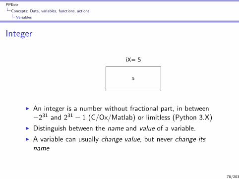
PPEctr
Concepts: Data, variables, functions, actions
Variables
Integer
iX= 5
5
I An integer is a number without fractional part, in between−231 and 231 − 1 (C/Ox/Matlab) or limitless (Python 3.X)
I Distinguish between the name and value of a variable.
I A variable can usually change value, but never change itsname
78/203

PPEctr
Concepts: Data, variables, functions, actions
Variables
Double
dX= 5.5
5.5
I A double (aka float) is a number with possibly a fractionalpart.
I Note that 5.0 is a double, while 5 is an integer.
I A computer is not ‘exact’, careful when comparing integersand doubles
I If you add a double to an integer, the result is double (inPython 3/Ox at least, language dependent)
[ Example: dAdd= 1/3; iD= 0; dD= iD + dAdd; type(dD) ]
79/203

PPEctr
Concepts: Data, variables, functions, actions
Variables
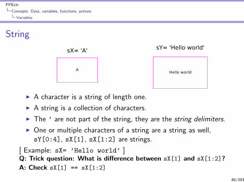
String
sX= 'A'
A
sY= 'Hello world'
Hello world
I A character is a string of length one.
I A string is a collection of characters.
I The ’ are not part of the string, they are the string delimiters.
I One or multiple characters of a string are a string as well,sY[0:4], sX[1], sX[1:2] are strings.
[ Example: sX= ’Hello world’ ]Q: Trick question: What is difference between sX[1] and sX[1:2]?
A: Check sX[1] == sX[1:2]
80/203
PPEctr
Concepts: Data, variables, functions, actions
Variables
String
sX= 'A'
A
sY= 'Hello world'
Hello world
I A character is a string of length one.
I A string is a collection of characters.
I The ’ are not part of the string, they are the string delimiters.
I One or multiple characters of a string are a string as well,sY[0:4], sX[1], sX[1:2] are strings.
[ Example: sX= ’Hello world’ ]Q: Trick question: What is difference between sX[1] and sX[1:2]?
A: Check sX[1] == sX[1:2]
80/203

PPEctr
Concepts: Data, variables, functions, actions
Variables
‘Simple’ types
I Boolean
I Integer
I Double/float
I String
Check type using
bX= True
type(bX)
81/203

PPEctr
Concepts: Data, variables, functions, actions
Variables
‘Difficult’ types
I List
I Tuple
I Matrix
I Function
I Lambda function
I DataFrame
I . . .
82/203

PPEctr
Concepts: Data, variables, functions, actions
Variables
List
lX= ['Beta', 5, [5.5]]
Beta 5 5.5
I A list is a collection of other objects.
I A list itself has one dimension, but can contain lists.
I An element of a list can be of any type (integer, double,function, matrix, list etc)
I A list of a list of a list has three dimensions etc.
I One may replace elements of a list (a list is mutable)
[ Example: lX= [’Beta’, 5, [5.5]]; lX[0]= ’Alpha’ ]
83/203
PPEctr
Concepts: Data, variables, functions, actions
Variables
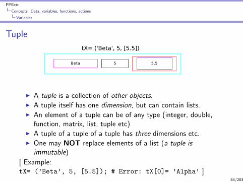
Tuple
tX= ('Beta', 5, [5.5])
Beta 5 5.5
I A tuple is a collection of other objects.I A tuple itself has one dimension, but can contain lists.I An element of a tuple can be of any type (integer, double,
function, matrix, list, tuple etc)I A tuple of a tuple of a tuple has three dimensions etc.I One may NOT replace elements of a list (a tuple is
immutable)
[ Example:tX= (’Beta’, 5, [5.5]); # Error: tX[0]= ’Alpha’ ]
84/203
PPEctr
Concepts: Data, variables, functions, actions
Variables
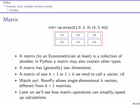
Matrix
mX= np.array([[1.0, 2, 3], [4, 5, 6]])
1.0 2.0 3.0
4.0 5.0 6.0
I A matrix (to an Econometrician at least) is a collection ofdoubles; in Python a matrix may also contain other types.
I A matrix has (generally) two dimensions.
I A matrix of size k × 1 or 1× k we tend to call a vector, vX
I Watch out: NumPy allows single-dimensional k vectors,different from k × 1 matrices.
I Later on we’ll see how matrix operations can simplify/speedup calculations.
85/203

PPEctr
Concepts: Data, variables, functions, actions
Variables
Matrix II
mX= np.array([[1.0, 2, 3], [4, 5, 6]])
1.0 2.0 3.0
4.0 5.0 6.0
In Python:
I we’ll use a list-of-lists as input into a NumPy array
I ensure we have doubles by making at least one of the entries adouble (here: 1.0), type(mX[1,2])
I if needed force it into a 2-dimensional shape,mX.shape= (6, 1)
[ Example: mX= np.array([[1.0, 2, 3], [4, 5, 6]]) ]
86/203

PPEctr
Concepts: Data, variables, functions, actions
Variables
Function
print ("Hello world")
print()
I A function performs a certain task, usually on a (number of)variables
I Hopefully the name of the function helps you to understandits task
I You can assign a function to a variable,fnMyPrintFunction= print
[ Example: fnMyPrintFunction(’Hello world’) ]
87/203

PPEctr
Concepts: Data, variables, functions, actions
Variables
Function II
Listing 31: pow6.pydef Pow(dBase , iPow):
dRes= 1
i= 0
while (i < iPow):
# print ("i= ", i)
dRes= dRes * dBase
i+= 1
return dRes
I You can define your own routines/functions
I You decide the output
I You tend to return the output
I (later: You may alter mutable arguments)
[ Example: dPow= Pow(2.0, 8) ]
88/203
PPEctr
Concepts: Data, variables, functions, actions
Variables
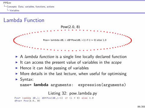
Lambda FunctionPow(2.0, 8)
Pow= lambda dB, i: dB*Pow(dB, i-1) if (i > 0) else 1.0
I A lambda function is a single line locally declared functionI It can access the present value of variables in the scopeI Hence it can hide passing of variablesI More details in the last lecture, when useful for optimisingI Syntax:
name= lambda arguments: expression(arguments)
Listing 32: pow lambda.pyPow= lambda dB,i: dB*Pow(dB,i-1) if (i > 0) else 1.0
dPow= Pow(2.0, 8)
89/203
PPEctr
Concepts: Data, variables, functions, actions
Variables
List comprehension
Alternative to a Lambda function can be a list comprehension, incertain cases. A list comprehension
I applies a function successively on all items in a list
I and returns the list of results
Structure:List = [ func(i) for i in somelist]
Examples:
[i for i in range (10)]
[i for i in range (10) if i%2 == 0]
[i**2 for i in range (10)]
[np.sqrt(mS2[i,i]) for i in range(iK)]
Q: Can you predict the outcome of each of these statements?
90/203

PPEctr
Concepts: Data, variables, functions, actions
Variables
DataFrame
I A Pandas dataframe is an object made for input/output ofdata
I It can be used to read/store/show your data
I And has plenty more options
I Very useful for data handling!
[ Example: import pandas as pd; lc= list(’ABC’);
df= pd.DataFrame(np.random.randn(4,3), columns=lc); df ]
91/203

PPEctr
Concepts: Data, variables, functions, actions
Variables
DataFrame II
Listing 33: stackols.pysData= ’data/stackloss.csv’
sY= ’Air Flow’
asX= [’Water Temperature ’, ’Acid Concentration ’, ’Stack Loss’]
# Initialisation
df= pd.read_csv(sData) # Read csv into dataframe
vY= df[sY]. values # Extract y-variable
mX= df[asX]. values # Extract x-variables
iN= vY.size # Check number of observations
mX= np.hstack ([np.ones((iN, 1)), mX]) # Append a vector of 1s
asX= [’constant ’]+asX
# Estimation
vBeta= np.linalg.lstsq(mX, vY)[0] # Run OLS y= X beta + e
# Output
print ("Ols estimates")
print (pd.DataFrame(vBeta , index=asX , columns =[’beta’]))
92/203

PPEctr
And other languages?
Python and other languagesConcepts are similar
I Python (and e.g. Ox/Gauss/Matlab) have automatic typing.Use it, but carefully...
I C/C++/Fortran need to have types and sizes specified at thestart. More difficult, but still same concept of variables.
I Precise manner for specifying a matrix differs from languageto language. Python needs some getting used to, but is(very...) flexible in the end
I Remember: An element has a value and a nameI A program moves the elements around, hopefully in a smart
manner
Keep track of your variables,know what is their type, size, and scope
93/203
PPEctr
And other languages?
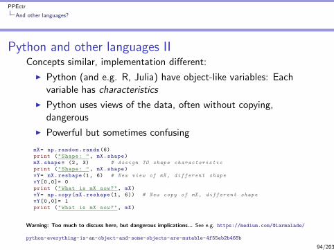
Python and other languages IIConcepts similar, implementation different:
I Python (and e.g. R, Julia) have object-like variables: Eachvariable has characteristics
I Python uses views of the data, often without copying,dangerous
I Powerful but sometimes confusing
mX= np.random.randn (6)
print ("Shape: ", mX.shape)
mX.shape= (2, 3) # Assign TO shape characteristic
print ("Shape: ", mX.shape)
vY= mX.reshape(1, 6) # New view of mX , different shape
vY[0,0]= 0
print ("What is mX now?", mX)
vY= np.copy(mX.reshape(1, 6)) # New copy of mX , different shape
vY[0,0]= 1
print ("What is mX now?", mX)
Warning: Too much to discuss here, but dangerous implications... See e.g. https://medium.com/@larmalade/
python-everything-is-an-object-and-some-objects-are-mutable-4f55eb2b468b
94/203

PPEctr
And other languages?
All languages
Programming is exact science
I Keep track of your variables
I Know what is their scope
I Program in small bits
I Program extremely structured
I Document your program wisely
I Think about algorithms, data storage, outcomes etc.
95/203

PPEctr
And other languages?
Scope
Further topics: Scope
Any variable is available only within the block in which it isdeclared.In practice:
1. Arguments to a function, e.g. mX in fnPrint( mX), areavailable within this function
2. A local variable mY is only known below its first use, withinthe present function
3. A global variable, indicated with global g_mZ at the start ofa function, and retains its value between functions.
96/203

PPEctr
And other languages?
Scope
Further topics: Scope
Any variable is available only within the block in which it isdeclared.In practice:
1. Arguments to a function, e.g. mX in fnPrint( mX), areavailable within this function
2. A local variable mY is only known below its first use, withinthe present function
3. A global variable, indicated with global g mZ at the start ofa function, and retains its value between functions.
96/203

PPEctr
And other languages?
Scope
Further topics: Scope II
Listing 34: scope global.oxdef localfunc ():
global g_sX
print ("In localfunc: g_sX= ", g_sX)
g_sX= "and goodbye" # Change the full global variable
# ##########################################################
### main
def main ():
global g_sX
g_sX= "Hello"
localfunc ()
print ("In main , after localfunc: g_sX= ", g_sX)
Rules for globals:
I Only use them when absolutely necessary (dangerous!)I Annotate them, g_I Fill them at last possible momentI Do not change them afterwards (unless absolutely necessary)
97/203
PPEctr
Afternoon Day 1
Afternoon session
Practical atVU UniversityMain building, HG 0B08 (EOR/QRM), 0B16 (TI-MPhil)13.30-16.00h
Topics:
I Regression: Simulate data
I Regression: Estimate model
98/203
PPEctr
Day 2
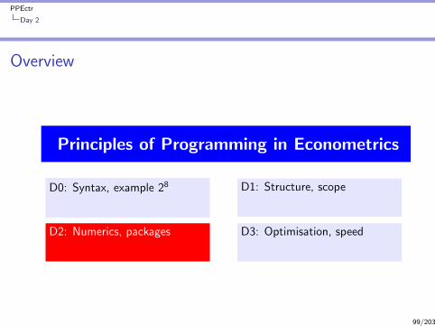
Overview
Principles of Programming in Econometrics
D0: Syntax, example 28 D1: Structure, scope
D2: Numerics, packages D3: Optimisation, speed
99/203
PPEctr
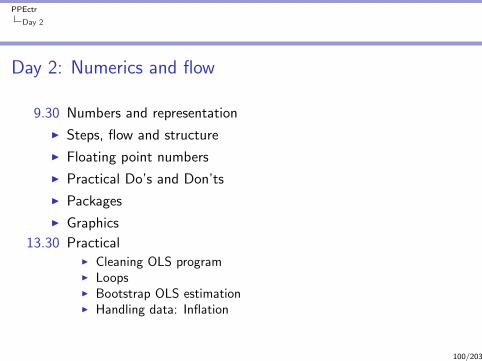
Day 2
Day 2: Numerics and flow
9.30 Numbers and representation
I Steps, flow and structure
I Floating point numbers
I Practical Do’s and Don’ts
I Packages
I Graphics
13.30 PracticalI Cleaning OLS programI LoopsI Bootstrap OLS estimationI Handling data: Inflation
100/203

PPEctr
Day 2
Reprise: What? Why?Wrong answer:
For the fun of it
A correct answer
To get to the results we need, in a fashion that iscontrollable, where we are free to implement the newestand greatest, and where we can be ‘reasonably’ sure ofthe answers
Data
HypothesisE= f(m)
ModelE= m c2
EstimationE²= m² (c²)2
0
1
1
1
1
1
1
10
1
1
0
0
1
1
Pro
gra
mm
ing
Science
101/203

PPEctr
Steps
Step P1: Analyse the dataI Read the original data fileI Make a first set of plots, look at itI Transform as necessary (aggregate, logs, first differences,
combine with other data sets)I Calculate statisticsI Save a file in a convenient format for later analysis
Data
HypothesisE= f(m)
ModelE= m c2
EstimationE²= m² (c²)2
0
1
1
1
1
1
1
10
1
1
0
0
1
1
Pro
gra
mm
ing
P1
mData= np.hstack ([vDate , mFX])
np.savez_compressed("data/fx9709.npz", mData)
df= pd.DataFrame(mData , columns =["Date", "UKUS", "EUUS", "JPUS"])
df.to_csv("data/fx9709.csv")
df.to_csv("data/fx9709.csv.gz",compression="gzip")
df.to_excel("data/fx9709.xlsx")
102/203

PPEctr
Steps
Step P2: Analyse the model
I Can you simulate data from the model?
I Does it look ‘similar’ to empirical data?
I Is it ‘the same’ type of input?
Data
HypothesisE= f(m)
ModelE= m c2
EstimationE²= m² (c²)2
0
1
1
1
1
1
1
10
1
1
0
0
1
1
Pro
gra
mm
ing
P2
mU= np.random.randn(iT, 4); # Log -returns US , UK , EU , JP factors
mF= np.cumsum(mU, axis =0); # Log -factors
mFX= np.exp(mF[:,1:]-mF [:.0]); # FX UK EU JP wrt US
103/203

PPEctr
Steps
Step P3: Estimate the model
I Take input (either empirical or simulated data)
I Implement model estimation
I Prepare useful outcome
Data
HypothesisE= f(m)
ModelE= m c2
EstimationE²= m² (c²)2
0
1
1
1
1
1
1
10
1
1
0
0
1
1
Pro
gra
mm
ing
P3
104/203
PPEctr
Steps
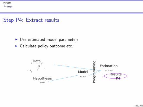
Step P4: Extract results
I Use estimated model parameters
I Calculate policy outcome etc.
Data
HypothesisE= f(m)
ModelE= m c2
EstimationE²= m² (c²)2
0
1
1
1
1
1
1
10
1
1
0
0
1
1
Pro
gra
mm
ing
ResultsP4
105/203

PPEctr
Steps
Step P5: Output
I Create tables/graphs
I Provide relevant output
Often this is the hardest part: What exactly did you want toknow? How can you look at the results? How can you go back tooriginal question, is this really the (correct) answer?
106/203

PPEctr
Steps
Result of stepsdef main ():
# Magic numbers
sData= "data/fx0017.csv" # Or use "data/sim0017.csv"
asFX= ["EUR/USD","GBP/USD","JPY/USD"]
vYY= [2000, 2015] # Years to analyse
# Initialise
(vDate , mRet)= ReadFX(asFX , vYY , sData)
# Estimate
(vP , vS , dLnPdf )= Estimate(mRet , asFX)
mFilt= ExtractResults(vP, mRet)
#Output
Output(vP, vS, dLnPdf , mFilt , asFX)
I Short mainI Starts off with setting items that might be changed: Only up
front in main (magic numbers)I Debug one part at a time (t.py)!I Easy for later re-use, if you write clean small blocks of codeI Input to estimation program is prepared data file, not raw
data (...).107/203

PPEctr
Flow
Program flow
Programming is (should be) no magic:
I Read your program. There is only one route the program willtake. You can follow it as well.
I Statements are executed in order, starting at main()
I A statement can call a function: The statements within thefunction are executed in order, until encountering a return
statement or the end of the function
I A statement can be a looping or conditional statement,repeating or skipping some statements. See below.
I (The order can also be broken by break or continuestatements. Don’t use, ugly.)
And that is all, any program follows these lines.(Sidenote: Objects/parallel programming etc)
108/203
PPEctr
Flow
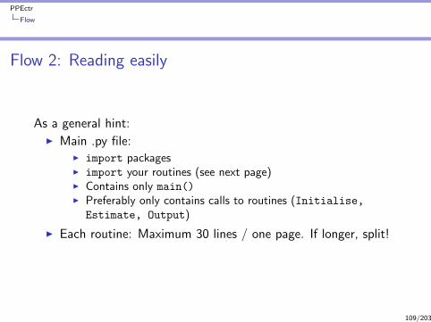
Flow 2: Reading easily
As a general hint:I Main .py file:
I import packagesI import your routines (see next page)I Contains only main()I Preferably only contains calls to routines (Initialise,
Estimate, Output)
I Each routine: Maximum 30 lines / one page. If longer, split!
109/203

PPEctr
Flow
Flow 3: Using modulesA module is a file containing a set of functions
All content from module incstack.py in directory lib can beimported by
from lib.incstack import *
Result: Nice short stackols3.py
Listing 35: stackols3.pyfrom lib.incstack import * # Import module with stackloss functions
# ##########################################################
### main
def main ():
# Magic numbers
...
# Initialisation
(vY , mX)= ReadStack(sData , sY, asX , True)
...
Q: What would be the difference between from
lib.incstack import * and import lib.incstack?In Spyder:
I check current directory (pwd), make sure that you are in your working directory (use cd if need be)I add general directory with modules to the PYTHONPATH, using Tools-PYTHONPATH manager
110/203
PPEctr
Flow
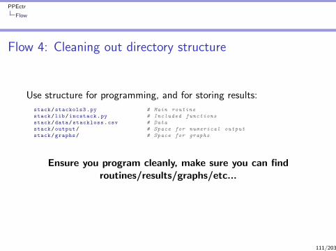
Flow 4: Cleaning out directory structure
Use structure for programming, and for storing results:
stack/stackols3.py # Main routine
stack/lib/incstack.py # Included functions
stack/data/stackloss.csv # Data
stack/output/ # Space for numerical output
stack/graphs/ # Space for graphs
Ensure you program cleanly, make sure you can findroutines/results/graphs/etc...
111/203

PPEctr
Floating point numbers and rounding errors
Precision
Not all numbers are made equal...Example: What is 1/3 + 1/3 + 1/3 + ...?
Listing 36: precision/onethird.pydef main ():
# Magic numbers
dD= 1/3
# Estimation
print ("i j sum diff");
dSum= 0.0
for i in range (10):
for j in range (3):
print (i, j, dSum , (dSum -i))
dSum+= dD # Successively add a third
See outcome: It starts going wrong after 16 digits...
112/203

PPEctr
Floating point numbers and rounding errors
Decimal or Binary
1-to-10 (Source: XKCD, http://xkcd.com/953/)
113/203
PPEctr
Floating point numbers and rounding errors
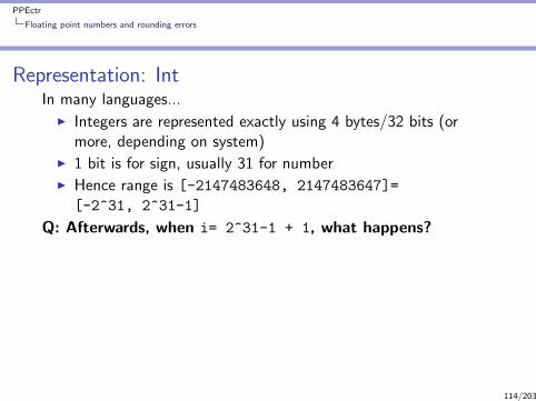
Representation: IntIn many languages...
I Integers are represented exactly using 4 bytes/32 bits (ormore, depending on system)
I 1 bit is for sign, usually 31 for numberI Hence range is [-2147483648, 2147483647]=
[-2^31, 2^31-1]
Q: Afterwards, when i= 2^31-1 + 1, what happens?
Answer:
I Ox: Circles around to a negative integer, without warning...I Matlab: Gets stuck at 2^31-1...I Python2: Uses 8 bytes, 64 bits. After 263 − 1, moves to long
type, without limitI Python3: long is the standard integer type, without any limit!
See precision/intmax.py
114/203

PPEctr
Floating point numbers and rounding errors
Representation: IntIn many languages...
I Integers are represented exactly using 4 bytes/32 bits (ormore, depending on system)
I 1 bit is for sign, usually 31 for numberI Hence range is [-2147483648, 2147483647]=
[-2^31, 2^31-1]
Q: Afterwards, when i= 2^31-1 + 1, what happens? Answer:
I Ox: Circles around to a negative integer, without warning...I Matlab: Gets stuck at 2^31-1...I Python2: Uses 8 bytes, 64 bits. After 263 − 1, moves to long
type, without limitI Python3: long is the standard integer type, without any limit!
See precision/intmax.py114/203
PPEctr
Floating point numbers and rounding errors
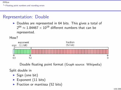
Representation: DoubleI Doubles are represented in 64 bits. This gives a total of
264 ≈ 1.84467× 10¹⁹ different numbers that can berepresented.
How?
Double floating point format (Graph source: Wikipedia)
Split double inI Sign (one bit)I Exponent (11 bits)I Fraction or mantissa (52 bits)
115/203
PPEctr
Floating point numbers and rounding errors
Representation: Double II
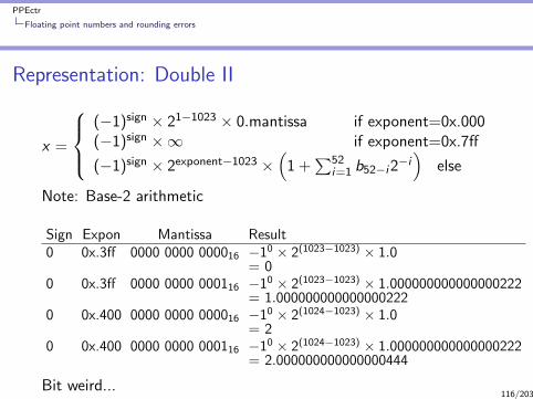
x =
(−1)sign × 21−1023 × 0.mantissa if exponent=0x.000(−1)sign ×∞ if exponent=0x.7ff
(−1)sign × 2exponent−1023 ×(
1 +∑52
i=1 b52−i2−i)
else
Note: Base-2 arithmetic
Sign Expon Mantissa Result0 0x.3ff 0000 0000 000016 −10 × 2(1023−1023) × 1.0
= 00 0x.3ff 0000 0000 000116 −10 × 2(1023−1023) × 1.000000000000000222
= 1.0000000000000002220 0x.400 0000 0000 000016 −10 × 2(1024−1023) × 1.0
= 20 0x.400 0000 0000 000116 −10 × 2(1024−1023) × 1.000000000000000222
= 2.000000000000000444
Bit weird...116/203
PPEctr
Floating point numbers and rounding errors
Consequence: Addition
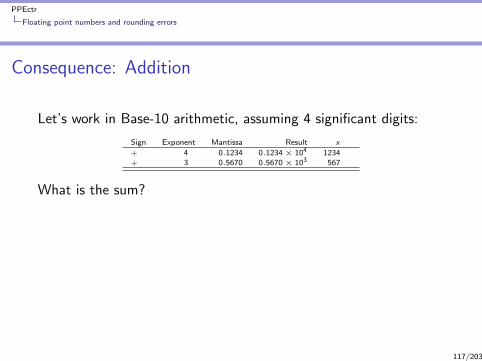
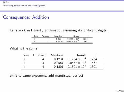
Let’s work in Base-10 arithmetic, assuming 4 significant digits:
Sign Exponent Mantissa Result x
+ 4 0.1234 0.1234 × 10⁴ 1234+ 3 0.5670 0.5670 × 10³ 567
What is the sum?
Sign Exponent Mantissa Result x+ 4 0.1234 0.1234× 10⁴ 1234+ 4 0.0567 0.0567× 10⁴ 567+ 4 0.1801 0.1801× 10⁴ 1801
Shift to same exponent, add mantissas, perfect
117/203
PPEctr
Floating point numbers and rounding errors
Consequence: Addition
Let’s work in Base-10 arithmetic, assuming 4 significant digits:
Sign Exponent Mantissa Result x
+ 4 0.1234 0.1234 × 10⁴ 1234+ 3 0.5670 0.5670 × 10³ 567
What is the sum?
Sign Exponent Mantissa Result x+ 4 0.1234 0.1234× 10⁴ 1234+ 4 0.0567 0.0567× 10⁴ 567+ 4 0.1801 0.1801× 10⁴ 1801
Shift to same exponent, add mantissas, perfect
117/203
PPEctr
Floating point numbers and rounding errors
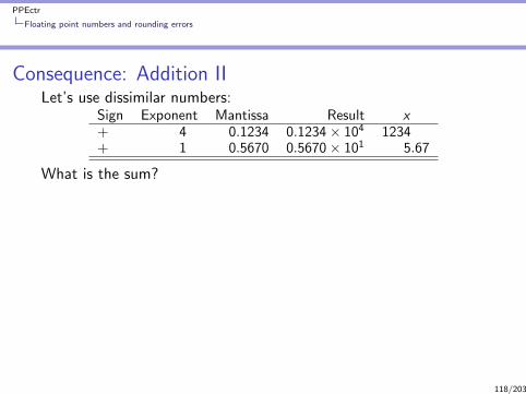
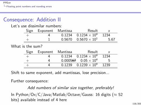
Consequence: Addition IILet’s use dissimilar numbers:
Sign Exponent Mantissa Result x+ 4 0.1234 0.1234× 10⁴ 1234+ 1 0.5670 0.5670× 101 5.67
What is the sum?
Sign Exponent Mantissa Result x+ 4 0.1234 0.1234× 10⁴ 1234+ 4 0.000567 0.05× 10⁴ 5+ 4 0.1239 0.1239× 10⁴ 1239
Shift to same exponent, add mantissas, lose precision...
Further consequence:
Add numbers of similar size together, preferably!
In Python/Ox/C/Java/Matlab/Octave/Gauss: 16 digits (≈ 52bits) available instead of 4 here
118/203
PPEctr
Floating point numbers and rounding errors
Consequence: Addition IILet’s use dissimilar numbers:
Sign Exponent Mantissa Result x+ 4 0.1234 0.1234× 10⁴ 1234+ 1 0.5670 0.5670× 101 5.67
What is the sum?
Sign Exponent Mantissa Result x+ 4 0.1234 0.1234× 10⁴ 1234+ 4 0.000567 0.05× 10⁴ 5+ 4 0.1239 0.1239× 10⁴ 1239
Shift to same exponent, add mantissas, lose precision...
Further consequence:
Add numbers of similar size together, preferably!
In Python/Ox/C/Java/Matlab/Octave/Gauss: 16 digits (≈ 52bits) available instead of 4 here
118/203

PPEctr
Floating point numbers and rounding errors
Consequence: Addition III
Check what happens in practice:
Listing 37: precision/accuracy.pydef main ():
dA= 0.123456 * 10**0
dB= 0.471132 * 10**15
dC= -dB
print ("a: ", dA, ", b: ", dB, ", c: ", dC)
print ("a + b + c: ", dA+dB+dC)
print ("a + (b + c): ", dA+(dB+dC))
print ("(a + b) + c: ", (dA+dB)+dC)
results ina: 0.123456 , b: 471132000000000.0 , c: -471132000000000.0
a + b + c: 0.125
a + (b + c): 0.123456
(a + b) + c: 0.125
119/203

PPEctr
Floating point numbers and rounding errors
Consequence: Addition III
Check what happens in practice:
Listing 38: precision/accuracy.pydef main ():
dA= 0.123456 * 10**0
dB= 0.471132 * 10**15
dC= -dB
print ("a: ", dA, ", b: ", dB, ", c: ", dC)
print ("a + b + c: ", dA+dB+dC)
print ("a + (b + c): ", dA+(dB+dC))
print ("(a + b) + c: ", (dA+dB)+dC)
results ina: 0.123456 , b: 471132000000000.0 , c: -471132000000000.0
a + b + c: 0.125
a + (b + c): 0.123456
(a + b) + c: 0.125
119/203
PPEctr
Floating point numbers and rounding errors
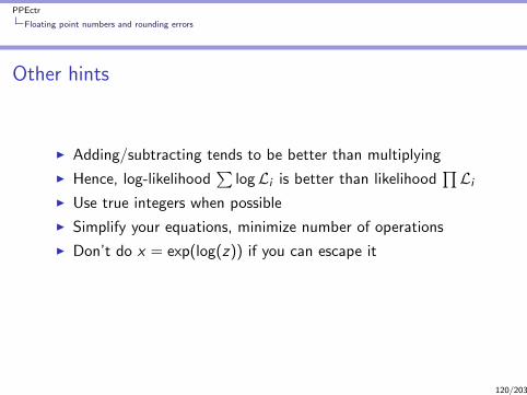
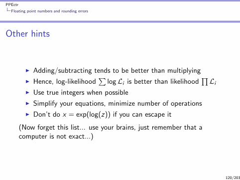
Other hints
I Adding/subtracting tends to be better than multiplying
I Hence, log-likelihood∑
logLi is better than likelihood∏Li
I Use true integers when possible
I Simplify your equations, minimize number of operations
I Don’t do x = exp(log(z)) if you can escape it
(Now forget this list... use your brains, just remember that acomputer is not exact...)
120/203
PPEctr
Floating point numbers and rounding errors
Other hints
I Adding/subtracting tends to be better than multiplying
I Hence, log-likelihood∑
logLi is better than likelihood∏Li
I Use true integers when possible
I Simplify your equations, minimize number of operations
I Don’t do x = exp(log(z)) if you can escape it
(Now forget this list... use your brains, just remember that acomputer is not exact...)
120/203

PPEctr
Do’s and Don’ts
Do’s and Don’tsThe do’s:
+ Use commenting through DocString for each routine,consistent style, and inline comments elsewhere if necessary
+ Use consistent indenting
+ Use Hungarian notation throughout (exception: countersi , j , k , l etc)
+ Define clearly what the purpose of a function is: One actionper function for clarity
+ Pass only necessary arguments to function
+ Analyse on paper before programming
+ Define debug possibilities, and use them
+ Order: Header – DocString – Code
+ Debug each bit (line...) of code after writing
121/203

PPEctr
Do’s and Don’ts
Do’s and Don’ts
The don’ts:
- Multipage functions
- Magic numbers in middle of program
- Use globals g vY when not necessary
- Unstructured, spaghetti-code
- Program using ‘write – write – write – debug’...
122/203
PPEctr
Import modules
import
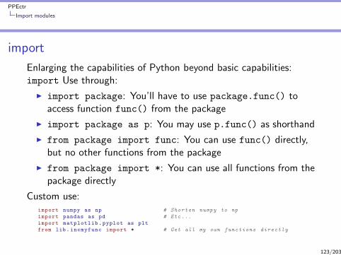
Enlarging the capabilities of Python beyond basic capabilities:import Use through:
I import package: You’ll have to use package.func() toaccess function func() from the package
I import package as p: You may use p.func() as shorthand
I from package import func: You can use func() directly,but no other functions from the package
I from package import *: You can use all functions from thepackage directly
Custom use:import numpy as np # Shorten numpy to np
import pandas as pd # Etc ...
import matplotlib.pyplot as plt
from lib.incmyfunc import * # Get all my own functions directly
123/203

PPEctr
Import modules
Python modules
Python packages
Package Purposenumpy Central, linear algebra and statistical operationsmatplotlib.pyplot Graphical capabilitiespandas Input/output, data analysis... Many others...
Warning: Use packages, but with care. How can you ascertain thatthe package computes exactly what you expect? Do youunderstand?
124/203

PPEctr
Import modules
Private modules
Private modules
I Convenient to package routines into modules, for use frommultiple (related) programs
I Stored in local project/lib directory, if only related to currentproject
I ... or stored at central python/lib directory: Use environmentvariable PYTHONPATH to tell Python where modules may befound; see Spyder – Tools – PYTHONPATH Manager
125/203

PPEctr
Graphics
A module: matplotlib.pyplotSeveral options available, here we focus on pyplot.
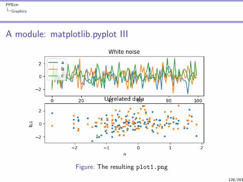
Listing 39: matplotlib/plot1.pyimport matplotlib.pyplot as plt
import numpy as np
# Initialisation
mY= np.random.randn (100, 3)
# Output
plt.figure(figsize =(8 ,4)) # Choose alternate size (def= (6.4 ,4.8))
plt.subplot(2, 1, 1) # Work with 2x1 grid , first plot
plt.plot(mY) # Simply plot the white noise
plt.legend (["a", "b", "c"]) # Add a legend
plt.title("White noise") # ... and a title
plt.subplot(2, 1, 2) # Start with second plot
plt.plot(mY[:,0], mY[:,1:], ".") # Plot here some cross -plots
plt.ylabel("b,c")
plt.xlabel("a")
plt.title("Unrelated data") # ... and name the graph
plt.savefig("graphs/plot1.png"); # Save the result
plt.show() # Done , show it
Details: matplotlib documentation, or e.g. Kevin Sheppard’sPython Introduction
126/203
PPEctr
Graphics
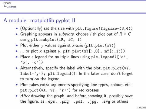
A module: matplotlib.pyplot III (Optionally) set the size with plt.figure(figsize=(8,4))
I Graphing appears in subplots, choose i ’th plot out of R × Cusing plt.subplot(iR, iC, i)
I Plot either y values against x-axis (plt.plot(mY))I ... or plot x against y , plt.plot(mY[:,0], mY[:,1:])
I Place a legend for multiple lines using plt.legend([’a’,
’b’, ’c’])
I Alternatively, specify the label with the plot, plt.plot(vY,label=’y’); plt.legend(). In the later case, don’t forgetto turn on the legend.
I Plot takes extra arguments specifying line types, colours etc:plt.plot(vX, vY, ’r+’) for red crosses
I After drawing the graph, and before showing it, possibly savethe figure, as .eps, .png, .pdf, .jpg, .svg or others
127/203
PPEctr
Graphics
A module: matplotlib.pyplot III
Figure: The resulting plot1.png
128/203
PPEctr
Graphics
Pandas + matplotlib
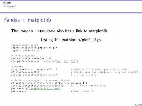
The Pandas DataFrame also has a link to matplotlib.
Listing 40: matplotlib/plot1 df.pyimport numpy as np
import matplotlib.pyplot as plt
import pandas as pd
# Initialisation
mY= np.random.randn (100, 3)
df= pd.DataFrame(mY , columns =["a", "b", "c"])
# Output
(fig , axes)= plt.subplots(2, 1) # Work with 2x1 grid , get link to axes
df.plot(ax=axes [0]) # Simply plot the dataframe , on first subplot
axes [0]. set_title("White noise") # ... and a title
# Build a cross -plot , in second subplot
df.plot(x="a", y=["b", "c"], style=".", ax=axes [1])
axes [1]. set_title("Unrelated data") # ... and a second title
plt.savefig("graphs/plot1_df.png")
plt.show() # Done , show it
129/203

PPEctr
Afternoon Day 2
Afternoon session
Practical atVU UniversityMain building, HG 0B08 (EOR/QRM), 0B16 (TI-MPhil)13.30-16.00h
Topics:
I Cleaning OLS program
I Loops
I Bootstrap OLS estimation
I Handling data
130/203

PPEctr
Day 3
Overview
Principles of Programming in Econometrics
D0: Syntax, example 28 D1: Structure, scope
D2: Numerics, packages D3: Optimisation, speed
131/203

PPEctr
Day 3
Day 3: Optimisation
9.30 Optimization (minimize)I Idea behind optimizationI Gauss-Newton/Newton-RaphsonI Stream/order of function calls
I Standard deviations
I Restrictions
I Speed
13.30 PracticalI Regression: Maximize likelihoodI GARCH-M: Intro and likelihood
132/203

PPEctr
Optimisation
OptimisationDoing Econometrics ≡ estimating models, e.g.:
1. Optimise likelihood
2. Minimise sum of squared residuals
3. Mimimise difference in moments
4. Solving utility problems (macro/micro)
5. Do Bayesian simulation, MCMC
Options 1-3 evolve around
θ = argminθ
f (y ; θ), f (y ; θ) : <k → <
Option 4 evolves around
r(y ; θ) ≡ 0, r(y ; θ) : <k → <k
133/203
PPEctr
Optimisation
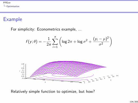
Example
For simplicity: Econometrics example, ...
f (y ; θ) = − 1
2n
n∑i=1
(log 2π + log σ2 +
(yi − µ)2
σ2
)
3.4 3.6
3.8 4
4.2 4.4
4.6 4.8
5
µ 1.4 1.6 1.8 2 2.2 2.4 2.6σ
-2.3
-2.25
-2.2
-2.15
-2.1
-2.05
-2
-1.95
f
Relatively simple function to optimize, but how?
134/203
PPEctr
Optimisation
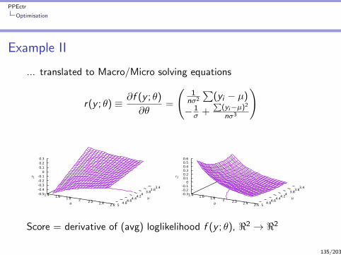
Example II
... translated to Macro/Micro solving equations
r(y ; θ) ≡ ∂f (y ; θ)
∂θ=
(1
nσ2
∑(yi − µ)
− 1σ +
∑(yi−µ)2
nσ3
)
3.4 3.6
3.8 4
4.2 4.4
4.6 4.8
5
µ 1.4 1.6 1.8 2 2.2 2.4 2.6σ
-0.5-0.4-0.3-0.2-0.1
0 0.1 0.2 0.3
r1
3.4 3.6
3.8 4
4.2 4.4
4.6 4.8
5
µ 1.4 1.6 1.8 2 2.2 2.4 2.6σ
-0.3-0.2-0.1
0 0.1 0.2 0.3 0.4 0.5 0.6
r2
Score = derivative of (avg) loglikelihood f (y ; θ), <2 → <2
135/203

PPEctr
Optimisation
Crawling up a hill
Step back and concentrate:
I Searching for
θ = argminθ f (y ; θ) = argmaxθ −f (y ; θ)
I How would you do that?
I Imagine Alps:
a. Step outside hotelb. What way goes up?c. Start Crawling up a hilld. Continue for a whilee. If not at top, go to b.
136/203

PPEctr
Optimisation
Crawling up a hill
Step back and concentrate:
I Searching for
θ = argminθ f (y ; θ) = argmaxθ −f (y ; θ)
I How would you do that?I Imagine Alps:
a. Step outside hotelb. What way goes up?c. Start Crawling up a hilld. Continue for a whilee. If not at top, go to b.
136/203
PPEctr
Optimisation
Use function characteristics
Translate to mathematics:
a. Set j = 0, start in some point θ(j)
b. Choose a direction s
c. Move distance α in that direction, θ(j+1) = θ(j) + αs
d. Increase j , and if not at top continue from b
Direction s: Linked to gradient?Minimum: Gradient 0, second derivative positive definite?(Maximum: Gradient 0, second derivative negative definite?)
137/203

PPEctr
Optimisation
Ingredients
Ingredients
Inputs are
I f , use (negative) average log likelihood, or averagesum-of-squares;
I Starting value θ(0);
I Possibly g = f ′, analytical first derivatives of f ;
I (and possibly H = f ′′, analytical second derivatives of f ).
or
I r , use set of equations, if necessary scaled;
I Starting value θ(0);
I If available J = r ′, analytical Jacobian of r
138/203
PPEctr
Optimisation
Ingredients
Ingredients II (optimize)
f (θ) : <k → < Function, scalar
f ′(θ) =
[∂f (θ)
∂θ1, . . . ,
∂f (θ)
∂θk
]T≡ g Derivative, gradient, k × 1
f ′′(θ) =
[∂2f (θ)
∂θi∂θj
]ki ,j=1
≡ H Second derivative, Hessian, k × k
If derivatives are continuous (as we assume), then
∂2f (θ)
∂θi∂θj=∂2f (θ)
∂θj∂θiH = HT
Hessian symmetric
139/203
PPEctr
Optimisation
Ingredients
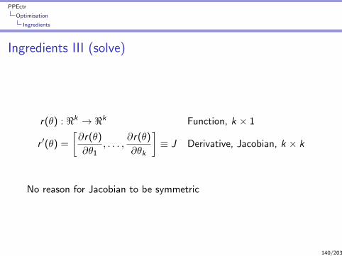
Ingredients III (solve)
r(θ) : <k → <k Function, k × 1
r ′(θ) =
[∂r(θ)
∂θ1, . . . ,
∂r(θ)
∂θk
]≡ J Derivative, Jacobian, k × k
No reason for Jacobian to be symmetric
140/203

PPEctr
Optimisation
Newton-Raphson and friends
Newton-Raphson for minimisation
I Approximate f (θ) locally with quadratic function
f (θ + h) ≈ q(h) = f (θ) + hT f ′(θ) +1
2hT f ′′(θ)h
I Minimise q(h) (instead of f (θ + h))
q′(h) = f ′(θ) + f ′′(θ)h = 0⇔ f ′′(θ)h = −f ′(θ) or Hh = −g
by solving last expression, h = −H−1g
I Set θ = θ + h, and repeat as necessary
Problems:
I Is H positive definite/invertible, at each step?
I Is step h, of length ||h||, too big or small?
I Do we converge to true solution?141/203

PPEctr
Optimisation
Newton-Raphson and friends
Newton-Raphson for solving equations
I Approximate r(y ; θ) locally with linear function
r(θ + h) ≈ q′(h) = r(θ) + r ′(θ)h
I Solve q′(h) = 0 (instead of r(θ + h) = 0)
q′(h) = r(θ) + r ′(θ)h = 0⇔ r ′(θ)h = −r(θ) or Jh = −r
by solving last expression, h = −J−1r
I Set θ = θ + h, and repeat as necessary
Problems:
I Is J negative definite/invertible, at each step?
I Is step h, of length ||h||, too big or small?
I Do we converge to true solution?142/203
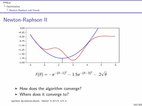
PPEctr
Optimisation
Newton-Raphson and friends
Newton-Raphson II
f (θ) = −e−(θ−1)2 − 1.5e−(θ−3)2 − .2√θ
I How does the algorithm converge?I Where does it converge to?
ipython np newton show2, theta= 5.9/1/0.1/0.4
143/203
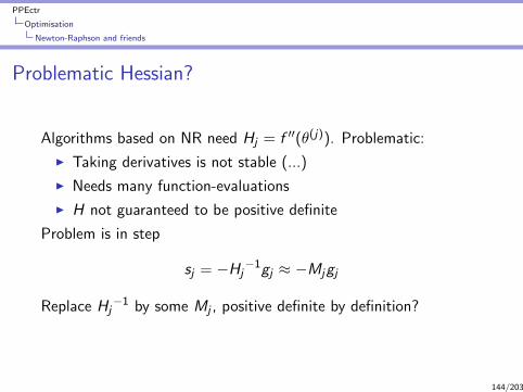
PPEctr
Optimisation
Newton-Raphson and friends
Problematic Hessian?
Algorithms based on NR need Hj = f ′′(θ(j)). Problematic:
I Taking derivatives is not stable (...)
I Needs many function-evaluations
I H not guaranteed to be positive definite
Problem is in step
sj = −Hj−1gj ≈ −Mjgj
Replace Hj−1 by some Mj , positive definite by definition?
144/203
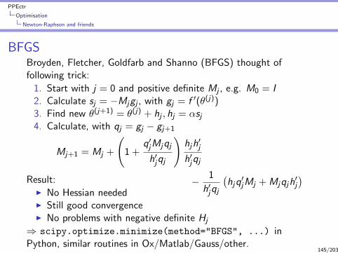
PPEctr
Optimisation
Newton-Raphson and friends
BFGSBroyden, Fletcher, Goldfarb and Shanno (BFGS) thought offollowing trick:
1. Start with j = 0 and positive definite Mj , e.g. M0 = I2. Calculate sj = −Mjgj , with gj = f ′(θ(j))3. Find new θ(j+1) = θ(j) + hj , hj = αsj4. Calculate, with qj = gj − gj+1
Mj+1 = Mj +
(1 +
q′jMjqj
h′jqj
)hjh′j
h′jqj
− 1
h′jqj
(hjq′jMj + Mjqjh
′j
)Result:
I No Hessian neededI Still good convergenceI No problems with negative definite Hj
⇒ scipy.optimize.minimize(method="BFGS", ...) inPython, similar routines in Ox/Matlab/Gauss/other.
145/203

PPEctr
Optimisation in practice
InputsInputs could be
I f , use (negative) average log likelihood, or averagesum-of-squares.
I Starting value θ0
I Possibly f ′, analytical first derivatives of f .
θ = argmaxθ
f (y ; θ), f (y ; θ) : <k → <
Or one could need
I Set of conditions to be solved,
I preferably nicely scaled,
r(y ; θ) ≡ 0, r(y ; θ) : <k → <k
146/203
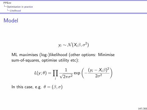
PPEctr
Optimisation in practice
Likelihood
Model
yi ∼ N (Xiβ, σ2)
ML maximises (log-)likelihood (other options: Minimisesum-of-squares, optimise utility etc):
L(y ; θ) =∏i
1√2πσ2
exp
(−(yi − Xiβ)2
2σ2
)In this case, e.g. θ = (β, σ)
147/203

PPEctr
Optimisation in practice
Likelihood
Function f
Write towards function f , to minimise:
log L(y ; θ) = −1
2
(n log 2π + n log σ2 +
1
σ2
∑(yi − Xiβ)2
)f (y ,X ; θ) =
1
2
(log 2π + log σ2 +
1
nσ2
∑(yi − Xiβ)2
)For testing:
I Work with generated data, e.g. n = 100, β =< 1, 1, 1 >′, σ =1,X = [1,U2,U3], y = Xβ + ε, ε ∼ N (0, σ2)
I Ensure you have the data...
148/203
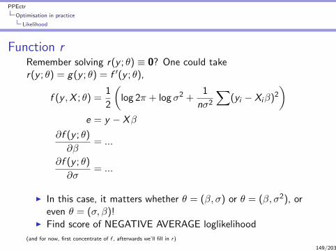
PPEctr
Optimisation in practice
Likelihood
Function rRemember solving r(y ; θ) ≡ 0? One could taker(y ; θ) = g(y ; θ) = f ′(y ; θ),
f (y ,X ; θ) =1
2
(log 2π + log σ2 +
1
nσ2
∑(yi − Xiβ)2
)e = y − Xβ
∂f (y ; θ)
∂β= ...
∂f (y ; θ)
∂σ= ...
I In this case, it matters whether θ = (β, σ) or θ = (β, σ2), oreven θ = (σ, β)!
I Find score of NEGATIVE AVERAGE loglikelihood
(and for now, first concentrate of f , afterwards we’ll fill in r)
149/203

PPEctr
Optimisation in practice
Likelihood
Comments of function
Listing 41: estnorm.py# ##########################################################
### dLL= LnLRegr(vP , vY , mX)
def LnLRegr(vP , vY , mX):
"""
Purpose:
Compute loglikelihood of regression model
Inputs:
vP iK+1 vector of parameters , with sigma and beta
vY iN vector of data
mX iN x iK matrix of regressors
Return value:
dLL double , loglikelihood
"""
Note: Full set of inputs including data. Parameters vP and vY both in 1D vector, mX as 2D matrix.
150/203
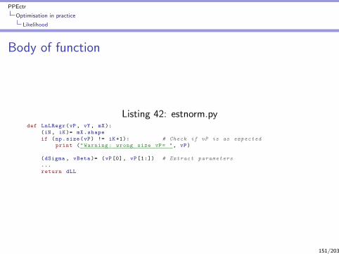
PPEctr
Optimisation in practice
Likelihood
Body of function
Listing 42: estnorm.pydef LnLRegr(vP , vY , mX):
(iN , iK)= mX.shape
if (np.size(vP) != iK+1): # Check if vP is as expected
print ("Warning: wrong size vP= ", vP)
(dSigma , vBeta)= (vP[0], vP[1:]) # Extract parameters
...
return dLL
151/203

PPEctr
Optimisation in practice
Likelihood
Body of function II
and fill in the remainder
Listing 43: estnorm.pydef LnLRegr(vP , vY , mX):
...
vE= vY - mX @ vBeta
vLL= -0.5*(np.log(2*np.pi) + 2*np.log(dSigma) + np.square(vE/dSigma ))
dLL= np.sum(vLL , axis= 0)
print (".", end="") # Give sign of life
return dLL
152/203

PPEctr
Optimisation in practice
Likelihood
Intermezzo: On robustness
WARNING:
I Check sizes of arguments to LL LnLRegr function carefully...
I Both y and θ should be 1D vectors, not 2D columns
I Calculate LL as dLL= np.sum(vLL, axis= 0), explicitlyalong axis 0
What could go wrong?
153/203
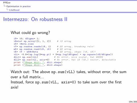
PPEctr
Optimisation in practice
Likelihood
Intermezzo: On robustness II
What could go wrong?
iN= 10; dSigma= 1;
vBeta= np.array([1, 1, 1]) # 1D array
iK= vBeta.size
vY= np.random.randn(iN, 1) # 2D array , breaking rule!
mX= np.random.rand(iN, iK) # 2D array
vE= vY - mX@vBeta # 2D array , shape (iN , iN)!
vLL= -0.5*(np.log(2*np.pi) + 2*np.log(dSigma) + np.square(vE/dSigma ))
dLL1= np.sum(vLL) # No error , nice scalar , but WRONG
dLL2= np.sum(vLL , axis =0) # No error , but 1D (iN ,) vector , detectable
print ("Shape dLL1: ", dLL1.shape)
print ("Shape dLL2: ", dLL2.shape)
Watch out: The above np.sum(vLL) takes, without error, the sumover a full matrix...Instead, force np.sum(vLL, axis=0) to take sum over the firstaxis!
154/203

PPEctr
Optimisation in practice
Likelihood
... And optimize? NO!Before you continue: Check the loglikelihood
I Does it work at all?
I Is the LL higher for a ‘good’ set of parameters, low for ‘bad’parameters?
I Is it reasonably efficient?
I How does it react to incorrect shape of parameters/data?
I How does it react to incorrect parameters (σ ≤ 0)?
Latter question, several options:
1. Don’t allow it, set dSigma= np.fabs(vP[0])
2. Flag that things go wrong: if (dSigma <= 0): return
-math.inf
3. Use constrained optimisation, e.g. Sequential Least SQuaresProgramming (SLSQP)
155/203
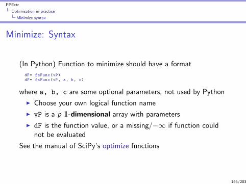
PPEctr
Optimisation in practice
Minimize syntax
Minimize: Syntax
(In Python) Function to minimize should have a format
dF= fnFunc(vP)
dF= fnFunc(vP, a, b, c)
where a, b, c are some optional parameters, not used by Python
I Choose your own logical function name
I vP is a p 1-dimensional array with parameters
I dF is the function value, or a missing/−∞ if function couldnot be evaluated
See the manual of SciPy’s optimize functions
156/203

PPEctr
Optimisation in practice
Minimize syntax
Minimize: Syntax II
No space for data? Negative average LL instead of positive LL?Use local Lambda function, providing the function to minimize as
Listing 44: estnorm.py# Create lambda function returning NEGATIVE AVERAGE LL , as function of vP only
AvgNLnLRegr= lambda vP: -LnLRegr(vP, vY, mX)/iN
Advantage:
I Simply return the negative of your previously preparedfunction, divided by n
I Value of data vY, mX at moment of call is passed along
I No globals needed!
Good alternative: Construct function AvgNLnLRegrXY(vP, vY, mX), and call opt.minimize(AvgNLnLRegr, vP0,
args=(vY, mX), method="BFGS")
157/203
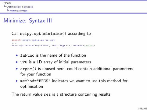
PPEctr
Optimisation in practice
Minimize syntax
Minimize: Syntax III
Call scipy.opt.minimize() according to
import scipy.optimize as opt
...
res= opt.minimize(fnFunc , vP0 , args=(), method="BFGS")
I fnFunc is the name of the function
I vP0 is a 1D array of initial parameters
I args=() is unused here, could contain additional parametersfor your function
I method="BFGS" indicates we want to use this method foroptimisation
The return value res is a structure containing results.
158/203

PPEctr
Optimisation in practice
Minimize syntax
Minimize: Syntax IV
After optimisation:
I Always check the outcome:
res= opt.minimize(AvgNLnLRegr , vP0 , args=(), method="BFGS")
vP= np.copy(res.x) # For safety , make a fresh copy
sMess= res.message
dLL= -iN*res.fun
print ("\nBFGS results in ", sMess , "\nPars: ", vP , "\nLL= ", dLL)
% print ("Full results: ", res)
I Possibly start thinking of using the outcome (standard errors,predictions, policy evaluation, robustness . . . )
159/203
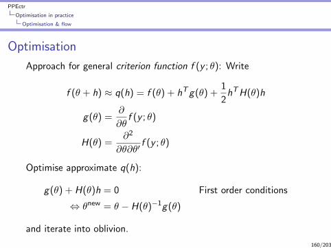
PPEctr
Optimisation in practice
Optimisation & flow
Optimisation
Approach for general criterion function f (y ; θ): Write
f (θ + h) ≈ q(h) = f (θ) + hTg(θ) +1
2hTH(θ)h
g(θ) =∂
∂θf (y ; θ)
H(θ) =∂2
∂θ∂θ′f (y ; θ)
Optimise approximate q(h):
g(θ) + H(θ)h = 0 First order conditions
⇔ θnew = θ − H(θ)−1g(θ)
and iterate into oblivion.
160/203
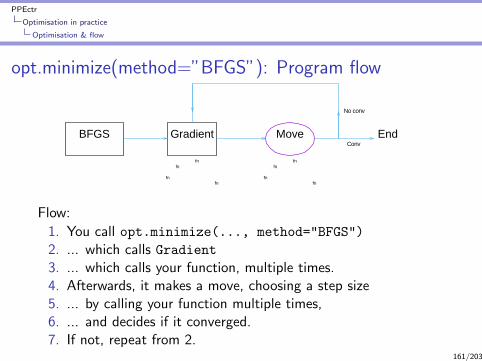
PPEctr
Optimisation in practice
Optimisation & flow
opt.minimize(method=”BFGS”): Program flow
BFGS Gradient Move EndConv
No conv
fnfn
fnfn
fnfn
fnfn
Flow:
1. You call opt.minimize(..., method="BFGS")
2. ... which calls Gradient
3. ... which calls your function, multiple times.4. Afterwards, it makes a move, choosing a step size5. ... by calling your function multiple times,6. ... and decides if it converged.7. If not, repeat from 2.
161/203

PPEctr
Optimisation in practice
Optimisation & flow
BFGS: Program flow II
Check out estnorm plot.py (k = 3, n = 100)
162/203

PPEctr
Optimisation in practice
Average loglikelihood
Minimize: Average
Why use average loglikelihood?
1. Likelihood function L(y ; θ) tends to have tiny values →possible problem with precision
2. Loglikelihood function log L(y ; θ) depends on number ofobservations: Large sample may lead to large |LL|, not stable
3. Average loglikelihood tends to be moderate in numbers,well-scaled...
Better from a numerical precision point-of-view.Warning:
Take care with score and standard errors (see later)
163/203

PPEctr
Optimisation in practice
Precision/convergence
Minimize: Precision
Optimisation is said to be successfull if (roughly):
1. ||g (j)(θ(j))|| ≤ gtol, with g (j) the score at θ(j), at iteration j :Scores are relatively small.
Note: Check 1 also depends on the scale of your function...Preferably f (θ) ≈ 1, not f (θ) ≈ 1e − 15!
Adapt the precision withres= opt.minimize(AvgNLnLRegr, vP0, args=(),
method="BFGS", tol= 1e-4),default is tol=1e-5.
164/203

PPEctr
Optimisation in practice
Score function
Minimize: Scores
-10
0
10
20
30
40
50
60
0.8 0.85 0.9 0.95 1 1.05 1.1 1.15 1.2
neg.LL x σ
Optimising ≡ ‘goingdown’≡ finding gradient.
Numerical gradient, for small h:
f ′(θ) =∂f (θ)
∂θ≈ f (θ + h)− f (θ)
h≈ f (θ + h)− f (θ − h)
2h
Function evaluations: 2× dim(θ)
Preferred: Analytical score f ′(θ)
165/203

PPEctr
Optimisation in practice
Score function
Minimize: Scores II
def AvgNLnLRegr_Jac(vP, vY , mX):
vSc= ???? # Compute analytical score
return vSc # return score , for NEGATIVE AVERAGE LL
I Provide a score function
I Work out vector of scores, of same size as θ.
I DEBUG! Check your score against opt.approx fprime()
166/203
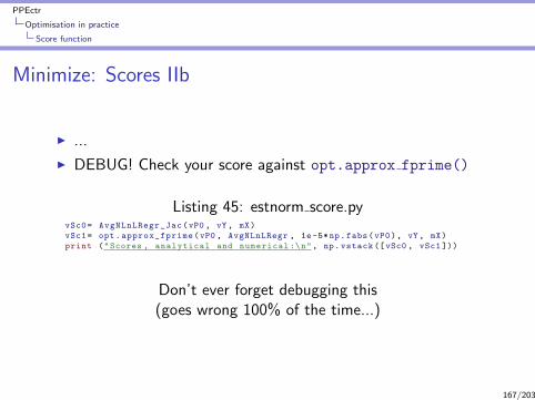
PPEctr
Optimisation in practice
Score function
Minimize: Scores IIb
I ...
I DEBUG! Check your score against opt.approx fprime()
Listing 45: estnorm score.pyvSc0= AvgNLnLRegr_Jac(vP0 , vY, mX)
vSc1= opt.approx_fprime(vP0 , AvgNLnLRegr , 1e-5*np.fabs(vP0), vY , mX)
print ("Scores , analytical and numerical :\n", np.vstack ([vSc0 , vSc1 ]))
Don’t ever forget debugging this(goes wrong 100% of the time...)
167/203
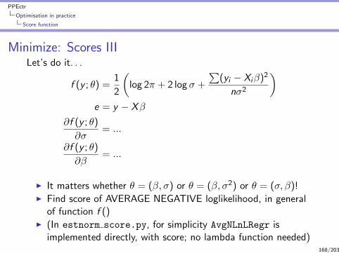
PPEctr
Optimisation in practice
Score function
Minimize: Scores IIILet’s do it. . .
f (y ; θ) =1
2
(log 2π + 2 log σ +
∑(yi − Xiβ)2
nσ2
)e = y − Xβ
∂f (y ; θ)
∂σ= ...
∂f (y ; θ)
∂β= ...
I It matters whether θ = (β, σ) or θ = (β, σ2) or θ = (σ, β)!I Find score of AVERAGE NEGATIVE loglikelihood, in general
of function f ()I (In estnorm score.py, for simplicity AvgNLnLRegr is
implemented directly, with score; no lambda function needed)168/203
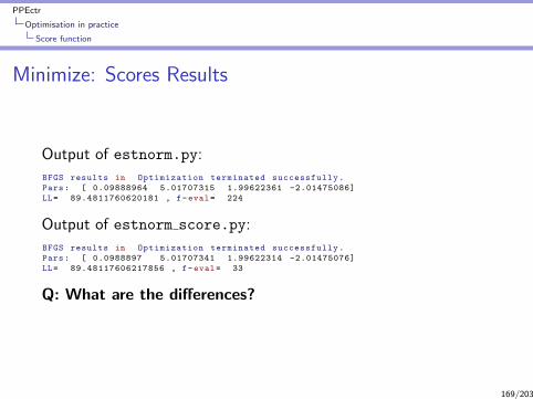
PPEctr
Optimisation in practice
Score function
Minimize: Scores Results
Output of estnorm.py:
BFGS results in Optimization terminated successfully.
Pars: [ 0.09888964 5.01707315 1.99622361 -2.01475086]
LL= 89.4811760620181 , f-eval= 224
Output of estnorm score.py:
BFGS results in Optimization terminated successfully.
Pars: [ 0.0988897 5.01707341 1.99622314 -2.01475076]
LL= 89.48117606217856 , f-eval= 33
Q: What are the differences?
169/203
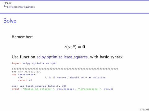
PPEctr
Solve nonlinear equations
Solve
Remember:
r(y ; θ) = 0
Use function scipy.optimize.least squares, with basic syntax
import scipy.optimize as opt
# ###################################################################
### vF= fnFunc0(vP)
def fnFunc0(vP):
vF= ... // k 1D vector , should be 0 at solution
return vF
res= opt.least_squares(fnFunc0 , x0)
print ("Nonlin LS returns ", res.message , "\nParameters ", res.x)
170/203
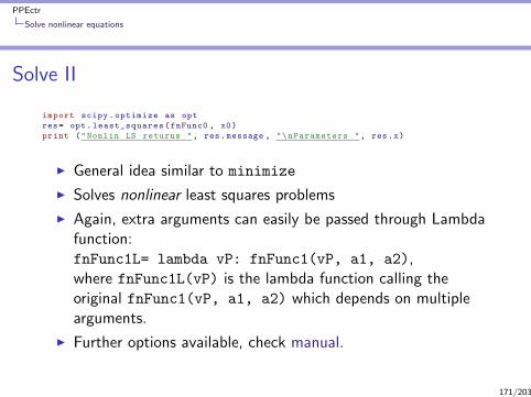
PPEctr
Solve nonlinear equations
Solve II
import scipy.optimize as opt
res= opt.least_squares(fnFunc0 , x0)
print ("Nonlin LS returns ", res.message , "\nParameters ", res.x)
I General idea similar to minimize
I Solves nonlinear least squares problems
I Again, extra arguments can easily be passed through Lambdafunction:fnFunc1L= lambda vP: fnFunc1(vP, a1, a2),where fnFunc1L(vP) is the lambda function calling theoriginal fnFunc1(vP, a1, a2) which depends on multiplearguments.
I Further options available, check manual.
171/203

PPEctr
Solve nonlinear equations
Example: Solve Macro
Given the parameters θ = (pH , ν1), depending on inputy = (σ1, σ2), a certain system describes the equilibrium in aneconomy if
r(y ; θ) =
p− 1σ1
H ν1 + p− 1σ2
H (1− ν1)− 2
pσ1−1σ1
H ν1 + ν1 − pH − 12
= 0.
For the solution to be sensible, it should hold that 0 < ν1 < 1 andpH 6= 0.If y = (2, 2), what are the optimal values of θ = (pH , ν1)?Solution: θ = (0.25, .5)
172/203

PPEctr
Standard deviations
Standard deviations
Given a model with
L(Y ; θ) Likelihood function
l(Y ; θ) = logL(Y ; θ) Log likelihood function
θ = argmaxθl(Y ; θ) ML estimator
what is the vector of standard deviations, σ(θ)?Assuming correct model specification,
Σ(θ) = −H(θ)−1
H(θ) =∂2l(Y ; θ)
∂θ∂θ′
⌋θ=θ
173/203

PPEctr
Standard deviations
SD2: Average likelihoodFor numerical stability, optimise average negative loglikelihood ln.For regression model, e.g. the stackloss model,
l(Y ; θ) = −(y − Xβ)′(y − Xβ)
2σ2− N log 2πσ2 + c
ln(Y ; θ) = −(y − Xβ)′(y − Xβ)
2Nσ2+ log 2πσ2 − c ′
Hln≡ ∂2ln(Y ; θ)
∂θ∂θ′= − 1
N
∂2l(Y ; θ)
∂θ∂θ′Σ(θ) =
1
N(Hln
)−1
Listing 46: opt/lib/incstack.pyres= opt.minimize(AvgNLnLRegr , vP0 , args=(vY , mX), method="BFGS")
mH= hessian_2sided(AvgNLnLRegr , res.x, vY, mX)
mS2= np.linalg.inv(mH)/iN
vS= np.sqrt(np.diag(mS2))
print ("\nBFGS results in ", res.message ,
"\nPars: ", res.x,
"\nLL= ", -iN*res.fun , ", f-eval= ", res.nfev)
174/203

PPEctr
Standard deviations
SD2: Hessian...
Hessian:
I is numerically unstable
I defines your standard errors
I hence is utterly important
I should be calculated with care!
But first: Check the gradient (simpler)
175/203

PPEctr
Standard deviations
SD2: Gradient...
Gradient:
g =∂f (θ)
∂θ≈ f (θ + h)− f (θ)
h≈ f (θ + h)− f (θ − h)
2h
I Central difference far more precise than forward difference
I Step size hi should depend on θi , different per element
I Rounding errors can become enormous, when h too small
I Python seems to provide scipy.optimize.approx fprime,forward difference
I ... and symbolic differentiation (better, slower, not pursuedhere)
⇒ lib/grad.py contains gradient 2sided()
176/203

PPEctr
Standard deviations
SD2: gradient 2sided
⇒ lib/grad.py contains gradient 2sided() (simplified here)
Listing 47: lib/grad.pydef gradient_2sided(fun , vP , *args):
iP = np.size(vP)
vP= vP.reshape(iP) # Ensure vP is 1D-array
vh = 1e-8*(np.fabs(vP)+1e-8) # Find stepsize
mh = np.diag(vh) # Build a diagonal matrix
fp = np.zeros(iP)
fm = np.zeros(iP)
for i in range(iP): # Find f(x+h), f(x-h)
fp[i] = fun(vP+mh[i], *args)
fm[i] = fun(vP-mh[i], *args)
vG= (fp - fm) / (2*vh) # Get central gradient
return vG
177/203
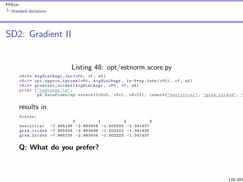
PPEctr
Standard deviations
SD2: Gradient II
Listing 48: opt/estnorm score.pyvSc0= AvgNLnLRegr_Jac(vP0 , vY, mX)
vSc1= opt.approx_fprime(vP0 , AvgNLnLRegr , 1e-5*np.fabs(vP0), vY , mX)
vSc2= gradient_2sided(AvgNLnLRegr , vP0 , vY, mX)
print ("\nScores :\n",
pd.DataFrame(np.vstack ([vSc0 , vSc1 , vSc2]), index=["Analytical", "grad_1sided", "grad_2sided"]))
results inScores:
0 1 2 3
Analytical -7.965135 -2.863504 -1.502223 -1.341437
grad_1sided -7.965005 -2.863499 -1.502222 -1.341435
grad_2sided -7.965135 -2.863504 -1.502223 -1.341437
Q: What do you prefer?
178/203
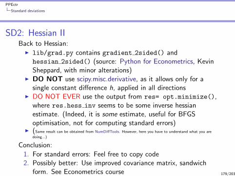
PPEctr
Standard deviations
SD2: Hessian IIBack to Hessian:
I lib/grad.py contains gradient 2sided() andhessian 2sided() (source: Python for Econometrics, KevinSheppard, with minor alterations)
I DO NOT use scipy.misc.derivative, as it allows only for asingle constant difference h, applied in all directions
I DO NOT EVER use the output from res= opt.minimize(),where res.hess inv seems to be some inverse hessianestimate. (Indeed, it is some estimate, useful for BFGSoptimisation, not for computing standard errors)
I (Same result can be obtained from NumDiffTools. However, here you have to understand what you are
doing...)
Conclusion:
1. For standard errors: Feel free to copy code2. Possibly better: Use improved covariance matrix, sandwich
form. See Econometrics course 179/203
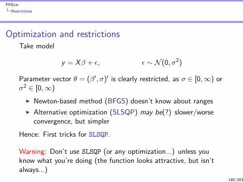
PPEctr
Restrictions
Optimization and restrictionsTake model
y = Xβ + ε, ε ∼ N (0, σ2)
Parameter vector θ = (β′, σ)′ is clearly restricted, as σ ∈ [0,∞) orσ2 ∈ [0,∞)
I Newton-based method (BFGS) doesn’t know about ranges
I Alternative optimization (SLSQP) may be(?) slower/worseconvergence, but simpler
Hence: First tricks for SLSQP.
Warning: Don’t use SLSQP (or any optimization...) unless youknow what you’re doing (the function looks attractive, but isn’talways...)
180/203
PPEctr
Restrictions
SLSQP
Restrictions: SLSQP
minimize(method="SLSQP") is an alternative tominimize(method="BFGS")
I Without restrictions, delivers results similar to BFGS
I Allows for sequential quadratic programming solution, forlinear and non-linear restrictions.
General call:res= opt.minimize(fun , vP0 , method="SLSQP", args=(),
bounds=tBounds , constraints=tCon)
181/203

PPEctr
Restrictions
SLSQP
SLSQP IIRestrictions:
1. bounds: Tuple of form tBounds= ((l0, u0), (l1, u1),
...) with lower and upper bounds per parameter (use None ifno restriction)
2. constraints: Tuple of dictionaries with entry ‘type’,indicating whether the function indicates an inequality(”ineq”) or equality (”eq”), and entry ‘fun’, giving a functionof a single argument which returns the constrained value. E.g.tCons= ({’type’: ’ineq’, ’fun’: fngt0},{’type’: ’eq’, ’fun’: fneq0})
Listing 49: estnorm slsqp.py/estnorm slsqp2.pytBounds= ((0, None),) + iK*((None , None),)
res= opt.minimize(AvgNLnLRegr , vP0 , method="SLSQP", bounds=tBounds)
# Or , alternatively
tCons= ({’type’: ’ineq’, ’fun’: fnsigmapos })
res= opt.minimize(AvgNLnLRegr , vP0 , method="SLSQP", constraints=tCons)
See manual for more details... 182/203

PPEctr
Restrictions
SLSQP
SLSQP III
Advantages:
I Simple
I Implements restrictions on parameter space (e.g.σ > 0, 0 < α + δ < 1)
Disadvantages:
I BFGS is meant for global optimisation; SLSQP might workworse
I Often better to incorporate restrictions in parametertransformation: Estimate θ = log σ,−∞ < θ <∞
So check out transformations...
183/203
PPEctr
Restrictions
Transforming parameters
Transforming parameters
Variance parameter positive?Solutions:
1. Use σ2 as parameter, have AvgLnLiklRegr return -math.infwhen negative σ2 is found
2. Use σ ≡ |θ0| as parameter, ie forget the sign altogether(doesn’t matter for optimisation, interpret negative σ inoutcome as positive value)
3. Transform, optimise θ∗0 = log σ ∈ (−∞,∞), no trouble foroptimisation
Last option most common, most robust, neatest.
184/203

PPEctr
Restrictions
Transforming parameters
Transform: Common transformations
Constraint θ∗ θ
[0,∞) log(θ) exp(θ∗)
[0, 1] log(
θ1−θ
)exp(θ∗)
1+exp(θ∗)
Of course, to get a range of [L,U], use a rescaled [0, 1]transformation.Note: See also exercise transpar
185/203

PPEctr
Restrictions
Transforming parameters
Transform: General solution
Distinguish θ = (σ, β′)′ and θ∗ = (log σ, β′)′. Steps:
I Get starting values θ
I Transform to θ∗
I Optimize θ∗, transforming back within LL routine
I Transform optimal θ∗ back to θ
Listing 50: opt/estnorm tr.py# Prepare wrapping function
def AvgNLnLiklRegrTr(vPTr , vY, mX):
vP= np.copy(vPTr) # Remember to COPY vPTr to a NEW variable
vP[0]= np.exp(vPTr [0])
return AvgNLnLiklRegr(vP, vY , mX)
...
vP0Tr= np.copy(vP0) # Remember to COPY vP0 to a NEW variable
vP0Tr [0]= np.log(vP0 [0])
res= opt.minimize(AvgNLnLRegrTr , vP0Tr , args=(vY , mX), method="BFGS")
vP= np.copy(res.x) # Remember to COPY x to a NEW variable
vP[0]= np.exp(vP[0]) # Remember to transform back!
186/203

PPEctr
Restrictions
Transforming parameters
Transform: Use functions
Notice code before: Transformations are performed
1. Before minimize
2. After minimize
3. Within AvgNLnLiklRegrTr
4. And probably more often for computing standard errors
Premium source for bugs... (see previous page: Two distinctimplementations for back-transform? Why?!?)
Solution: Define
I vPTr= TransPar(vP): θ → θ∗
I vP= TransBackPar(vPTr) θ∗ → θ
And test (in a separate program) whether transformation worksright. Necessary when using multiple transformed parameters.
187/203

PPEctr
Restrictions
Transforming parameters
Transform: Use functions II
Listing 51: opt/estnorm tr3.py# Use lambda function to transform back in place
AvgNLnLRegrTr= lambda vPTr , vY , mX: AvgNLnLRegr(TransBackPar(vPTr), vY, mX)
vP0Tr= TransPar(vP0)
res= opt.minimize(AvgNLnLRegrTr , vP0Tr , args=(vY , mX), method="BFGS")
vP= TransBackPar(res.x) # Remember to transform back!
188/203
PPEctr
Restrictions
Transforming parameters
Standard deviations
Remember:
Σ(θ) = −H(θ)−1
H(θ) =δ2l(Y ; θ)
δθδθ′
⌋θ=−θ
= Nδ2ln(Y ; θ)
δθδθ′
⌋θ=θ
Therefore, we need (average negative) loglikelihood in terms of θ,not θ∗ for sd’s...
189/203
PPEctr
Restrictions
Transforming parameters
Transforming parameters II: SDQuestion: How to construct standard deviations?Answers:
1. Use transformation in estimation, not in calculation ofstandard deviation. Advantage: Simpler. Disadvantage:Troublesome when parameter close to border.
2. Use transformation throughout, use Delta-method to computestandard errors. Advantage: Fits with theory. Disadvantage:Is standard deviation of σ informative, is its likelihoodsufficiently peaked/symmetric?
3. After estimation, compute bootstrap standard errors4. Who needs standard errors? Compute 95% bounds on θ∗,
translate those to 95% bounds on parameter θ. Advantage:Theoretically nicer. Disadvantage: Not everybody understandsadvantage.
See next slides.190/203
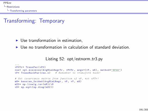
PPEctr
Restrictions
Transforming parameters
Transforming: Temporary
I Use transformation in estimation,
I Use no transformation in calculation of standard deviation.
Listing 52: opt/estnorm tr3.py...
vP0Tr= TransPar(vP0)
res= opt.minimize(AvgNLnLRegrTr , vP0Tr , args=(vY , mX), method="BFGS")
vP= TransBackPar(res.x) # Remember to transform back!
# Get covariance matrix from function of vP , not vPTr!
mH= hessian_2sided(AvgNLnLRegr , vP, vY, mX)
mS2= np.linalg.inv(mH)/iN
vS= np.sqrt(np.diag(mS2))
191/203

PPEctr
Restrictions
Transforming parameters
Transforming: Delta
n1/2(θ∗ − θ∗0)a∼ N
(0,V∞(θ∗)
)θ = g(θ∗)
θ ≈ g(θ∗0) + g ′(θ∗0)(θ∗ − θ∗0)
n1/2(θ − θ0)a= g ′0n
1/2(θ∗ − θ∗0)a∼ N (0, (g ′0)2V∞(θ∗)) scalar
n1/2(θ − θ0)a∼ N (0,G0V
∞(θ∗)G ′0) vector
In practice: Use
var(θ) = G var(θ∗)G ′
G =δg(θ∗)
δθ∗′=(dg(θ∗)dθ∗1
dg(θ∗)dθ∗2
· · · dg(θ∗)dθ∗k
)= Jacobian
192/203
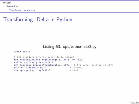
PPEctr
Restrictions
Transforming parameters
Transforming: Delta in Python
Listing 53: opt/estnorm tr3.pyvPTr= res.x
# Get standard errors , using delta method
mH= hessian_2sided(AvgNLnLRegrTr , vPTr , vY, mX)
mS2Th= np.linalg.inv(mH)/iN
mG= jacobian_2sided(TransBackPar , vPTr) # Evaluate jacobian at vPTr
mS2= mG @ mS2Th @ mG.T # Cov(vP)
vS= np.sqrt(np.diag(mS2)) # s(vP)
193/203

PPEctr
Restrictions
Transforming parameters
Transforming: Bootstrap
I Estimate model, resulting in θ = g(θ∗)
I From the model, generate j = 1, ..,B bootstrap samples
y(j)s (θ)
I For each sample, estimate θ(j)s = g(θ∗
(j)s )
I Report var(θ) = var(θ(1)s , . . . , θ
(B)s )
I.e, report variance/standard deviation among those B estimates ofthe parameters, assuming your parameter estimates are used in theDGP.
Simple, somewhat computer-intensive?
194/203
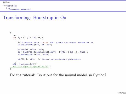
PPEctr
Restrictions
Transforming parameters
Transforming: Bootstrap in Ox
{
...
for (j= 0; j < iB; ++j)
{
// Simulate data Y from DGP , given estimated parameter vP
GenerateData (&vY, mX , vP);
TransPar (&vPTr , vP);
ir= MaxBFGS(fnAvgLnLiklRegrTr , &vPTr , &dLL , 0, TRUE);
TransBackPar (&vPB , vPTr);
mG[][j]= vPB; // Record re-estimated parameters
}
mS2= variance(mG’);
avS [0]= sqrt(diagonal(mS2)’);
}
For the tutorial: Try it out for the normal model, in Python?
195/203

PPEctr
Speed
Speed
Elements to consider
I Use matrices, avoid loops
I Adapt large matrices in-place
I Use built-in functions
I Optimise inner loop
I Avoid using ‘hat’ matrices/outer products over largedimensions
I Link in C or Fortran code
I Use Numba or Cython
196/203

PPEctr
Speed
Loops
Speed: Loops vs matrices
Avoid loops like the plague.Most of the time there is a matrix alternative, like for constructingdummies:
Listing 54: speed loop2.pyiN= 10000
iR= 1000
vY= np.random.randn(iN, 1)
vDY= np.zeros_like(vY)
with Timer("Loop"):
for r in range(iR):
for i in range(iN):
if (vY[i] > 0):
vDY[i]= 1
else:
vDY[i]= -1
with Timer("Matrix"):
for r in range(iR):
vDY= np.ones_like(vY)
vDY[vY <= 0]= 1
197/203

PPEctr
Speed
Argument vs return
Speed: Argument vs return
Listing 55: speed argument.pydef funcret(mX):
(iN , iK)= mX.shape
mY= np.random.randn(iN, iK)
return mY
def funcarg(mX):
(iN , iK)= mX.shape
mX[:,:]= np.random.randn(iN, iK)
def main ():
...
mX= np.zeros((iN, iK))
with Timer("return"):
for r in range(iR):
mX= funcret(mX)
with Timer("argument"):
for r in range(iR):
funcarg(mX)
Note: No true difference to be found, good memory management...
198/203

PPEctr
Speed
Functions
Speed: Built-in functions
Listing 56: speed builtin.pydef MyOls(vY, mX):
vB= np.linalg.inv(mX.T@mX)@mX.T@vY
return vB
def main ():
...
with Timer("MyOls"):
for r in range(iR):
vB= MyOls(vY, mX)
with Timer("lstsq"):
for r in range(iR):
vB= np.linalg.lstsq(mX, vY, rcond=None )[0]
Note: This function lstsq is even slower... More stable in awkward situations...
199/203

PPEctr
Speed
Concatenation
Speed: Concatenation or predefine
In a simulation with a matrix of outcomes, predefine the matrix tobe of the correct size, then fill in the rows.The other option, concatenating rows to previous results, takes alot longer.
Listing 57: speed concat.pyiN= 1000
iK= 1000
mX= np.empty((0, iK))
with Timer("concat"):
for j in range(iN):
mX= np.vstack ([mX, np.random.randn(1, iK)])
mX= np.empty((iN, iK))
with Timer("predef"):
for j in range(iN):
mX[j,:]= np.random.randn(1, iK)
200/203
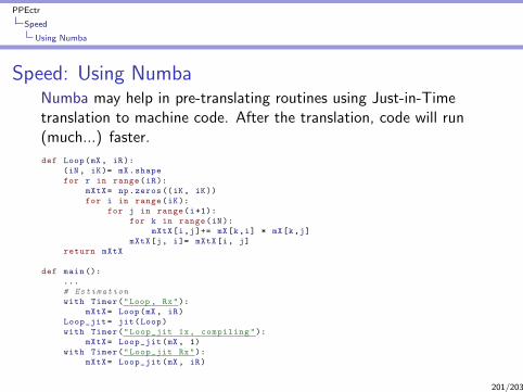
PPEctr
Speed
Using Numba
Speed: Using NumbaNumba may help in pre-translating routines using Just-in-Timetranslation to machine code. After the translation, code will run(much...) faster.
def Loop(mX, iR):
(iN , iK)= mX.shape
for r in range(iR):
mXtX= np.zeros((iK, iK))
for i in range(iK):
for j in range(i+1):
for k in range(iN):
mXtX[i,j]+= mX[k,i] * mX[k,j]
mXtX[j, i]= mXtX[i, j]
return mXtX
def main ():
...
# Estimation
with Timer("Loop , Rx"):
mXtX= Loop(mX, iR)
Loop_jit= jit(Loop)
with Timer("Loop_jit 1x, compiling"):
mXtX= Loop_jit(mX, 1)
with Timer("Loop_jit Rx"):
mXtX= Loop_jit(mX, iR)
201/203

PPEctr
Speed
Overview
Speed: Overview
Conclusions:
I If your program takes more than a few seconds, optimise
I Track the time spent in functions, optimise what takes longest
I Don’t concatenate/stack
I Use matrix-operations/vectorized code instead of loops
I Look into Numba for loop-heavy code
I Use Cython (not covered here), or move to Julia, (not coveredhere) for computationally intensive stuff
202/203

PPEctr
Speed
Overview
Closing thoughts
And so, the course comes to an end...Please
I keep concepts, principles of programming, in mind
I structure your programs wisely
On a voluntary basis:
I in groups of max 2
I before Monday September 30, 9.00AMI hand in a solution to
1. GARCH-ML problem (similar to OLS exercise, minorextensions)
2. BinTree problem (relevant to QRM students, nice setting forothers)
(see Canvas for details)
203/203