Principles of Programming Languages Declarative ...arusoaie.andrei/... · Principles of Programming...
106
Principles of Programming Languages Declarative programming: functional programming Andrei Arusoaie 1 1 Department of Computer Science January 9, 2020
Transcript of Principles of Programming Languages Declarative ...arusoaie.andrei/... · Principles of Programming...
Principles of Programming LanguagesDeclarative programming: functional
programming
Andrei Arusoaie1
1Department of Computer Science
January 9, 2020

Outline
Paradigms
Declarative ProgrammingFunctional Programming
Conclusion
Outline
Paradigms
Declarative ProgrammingFunctional Programming
Conclusion
Outline
Paradigms
Declarative ProgrammingFunctional Programming
Conclusion

Paradigms
I Imperative Programming:
I Object Oriented Programming:I Declarative Programming
I Functional ProgrammingI Logic Programming
Paradigms
I Imperative Programming:I Object Oriented Programming:
I Declarative ProgrammingI Functional ProgrammingI Logic Programming
Paradigms
I Imperative Programming:I Object Oriented Programming:I Declarative Programming
I Functional ProgrammingI Logic Programming
Outline
Paradigms
Declarative ProgrammingFunctional Programming
Conclusion

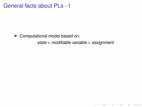
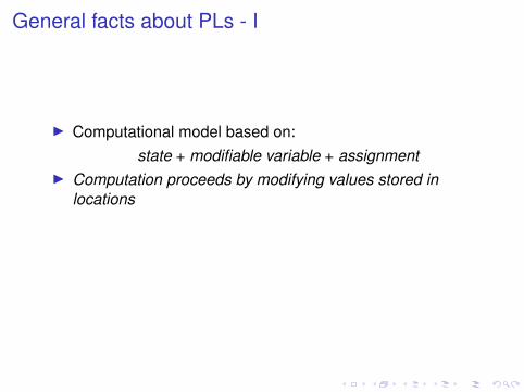
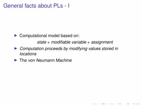
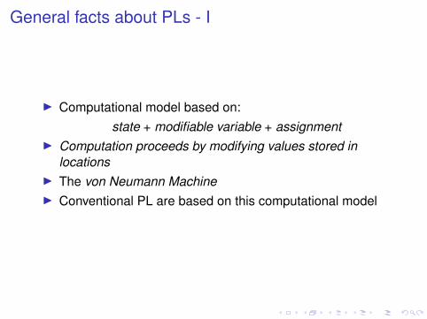
General facts about PLs - I
I Computational model based on:state + modifiable variable + assignment
I Computation proceeds by modifying values stored inlocations
I The von Neumann MachineI Conventional PL are based on this computational model
General facts about PLs - I
I Computational model based on:state + modifiable variable + assignment
I Computation proceeds by modifying values stored inlocations
I The von Neumann MachineI Conventional PL are based on this computational model
General facts about PLs - I
I Computational model based on:state + modifiable variable + assignment
I Computation proceeds by modifying values stored inlocations
I The von Neumann MachineI Conventional PL are based on this computational model
General facts about PLs - I
I Computational model based on:state + modifiable variable + assignment
I Computation proceeds by modifying values stored inlocations
I The von Neumann Machine
I Conventional PL are based on this computational model
General facts about PLs - I
I Computational model based on:state + modifiable variable + assignment
I Computation proceeds by modifying values stored inlocations
I The von Neumann MachineI Conventional PL are based on this computational model
General facts about PLs - II
I However, this is not the only possible model upon which tobase a PL
:I It is possible to compute without referring to a state. How?I ... by rewriting expressionsI The computation is expressed in terms of modifications of
the environmentI “Pure” principles: do not modify the ‘state’; no side-effects
General facts about PLs - II
I However, this is not the only possible model upon which tobase a PL:I It is possible to compute without referring to a state
. How?I ... by rewriting expressionsI The computation is expressed in terms of modifications of
the environmentI “Pure” principles: do not modify the ‘state’; no side-effects
General facts about PLs - II
I However, this is not the only possible model upon which tobase a PL:I It is possible to compute without referring to a state. How?
I ... by rewriting expressionsI The computation is expressed in terms of modifications of
the environmentI “Pure” principles: do not modify the ‘state’; no side-effects
General facts about PLs - II
I However, this is not the only possible model upon which tobase a PL:I It is possible to compute without referring to a state. How?I ... by rewriting expressions
I The computation is expressed in terms of modifications ofthe environment
I “Pure” principles: do not modify the ‘state’; no side-effects
General facts about PLs - II
I However, this is not the only possible model upon which tobase a PL:I It is possible to compute without referring to a state. How?I ... by rewriting expressionsI The computation is expressed in terms of modifications of
the environment
I “Pure” principles: do not modify the ‘state’; no side-effects
General facts about PLs - II
I However, this is not the only possible model upon which tobase a PL:I It is possible to compute without referring to a state. How?I ... by rewriting expressionsI The computation is expressed in terms of modifications of
the environmentI “Pure” principles: do not modify the ‘state’; no side-effects
Functional programming: history + characteristics
I This paradigm is as old as the imperative one
I Turing machine vs. λ-calculusI Ingredients: higher-order functions + recursionI PLs: Haskell, Miranda (pure) + Lisp, ML, Scheme, . . .
Functional programming: history + characteristics
I This paradigm is as old as the imperative oneI Turing machine vs. λ-calculus
I Ingredients: higher-order functions + recursionI PLs: Haskell, Miranda (pure) + Lisp, ML, Scheme, . . .
Functional programming: history + characteristics
I This paradigm is as old as the imperative oneI Turing machine vs. λ-calculusI Ingredients: higher-order functions + recursion
I PLs: Haskell, Miranda (pure) + Lisp, ML, Scheme, . . .
Functional programming: history + characteristics
I This paradigm is as old as the imperative oneI Turing machine vs. λ-calculusI Ingredients: higher-order functions + recursionI PLs: Haskell, Miranda (pure) + Lisp, ML, Scheme, . . .
Some mathematical background
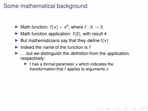
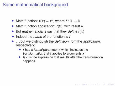
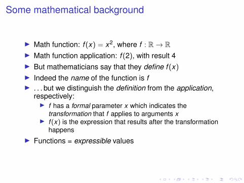
I Math function: f (x) = x2
, where f : R→ RI Math function application: f (2), with result 4I But mathematicians say that they define f (x)I Indeed the name of the function is fI . . . but we distinguish the definition from the application,
respectively:I f has a formal parameter x which indicates the
transformation that f applies to arguments xI f (x) is the expression that results after the transformation
happensI Functions = expressible values
Some mathematical background
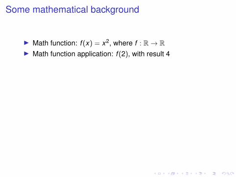
I Math function: f (x) = x2, where f : R→ R
I Math function application: f (2), with result 4I But mathematicians say that they define f (x)I Indeed the name of the function is fI . . . but we distinguish the definition from the application,
respectively:I f has a formal parameter x which indicates the
transformation that f applies to arguments xI f (x) is the expression that results after the transformation
happensI Functions = expressible values
Some mathematical background
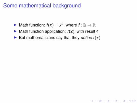
I Math function: f (x) = x2, where f : R→ RI Math function application: f (2), with result 4
I But mathematicians say that they define f (x)I Indeed the name of the function is fI . . . but we distinguish the definition from the application,
respectively:I f has a formal parameter x which indicates the
transformation that f applies to arguments xI f (x) is the expression that results after the transformation
happensI Functions = expressible values
Some mathematical background
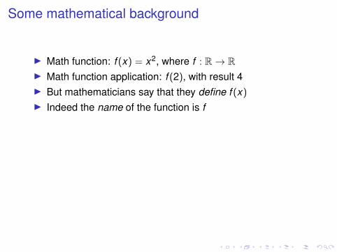
I Math function: f (x) = x2, where f : R→ RI Math function application: f (2), with result 4I But mathematicians say that they define f (x)
I Indeed the name of the function is fI . . . but we distinguish the definition from the application,
respectively:I f has a formal parameter x which indicates the
transformation that f applies to arguments xI f (x) is the expression that results after the transformation
happensI Functions = expressible values
Some mathematical background
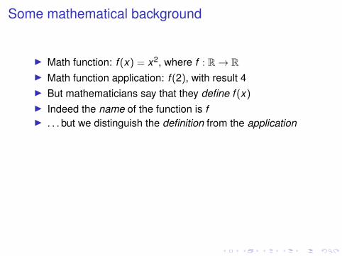
I Math function: f (x) = x2, where f : R→ RI Math function application: f (2), with result 4I But mathematicians say that they define f (x)I Indeed the name of the function is f
I . . . but we distinguish the definition from the application,respectively:I f has a formal parameter x which indicates the
transformation that f applies to arguments xI f (x) is the expression that results after the transformation
happensI Functions = expressible values
Some mathematical background
I Math function: f (x) = x2, where f : R→ RI Math function application: f (2), with result 4I But mathematicians say that they define f (x)I Indeed the name of the function is fI . . . but we distinguish the definition from the application
,respectively:I f has a formal parameter x which indicates the
transformation that f applies to arguments xI f (x) is the expression that results after the transformation
happensI Functions = expressible values
Some mathematical background
I Math function: f (x) = x2, where f : R→ RI Math function application: f (2), with result 4I But mathematicians say that they define f (x)I Indeed the name of the function is fI . . . but we distinguish the definition from the application,
respectively:I f has a formal parameter x which indicates the
transformation that f applies to arguments x
I f (x) is the expression that results after the transformationhappens
I Functions = expressible values
Some mathematical background
I Math function: f (x) = x2, where f : R→ RI Math function application: f (2), with result 4I But mathematicians say that they define f (x)I Indeed the name of the function is fI . . . but we distinguish the definition from the application,
respectively:I f has a formal parameter x which indicates the
transformation that f applies to arguments xI f (x) is the expression that results after the transformation
happens
I Functions = expressible values
Some mathematical background
I Math function: f (x) = x2, where f : R→ RI Math function application: f (2), with result 4I But mathematicians say that they define f (x)I Indeed the name of the function is fI . . . but we distinguish the definition from the application,
respectively:I f has a formal parameter x which indicates the
transformation that f applies to arguments xI f (x) is the expression that results after the transformation
happensI Functions = expressible values
More about writing function application
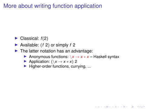
I Classical: f (2)
I Available: (f 2) or simply f 2I The latter notation has an advantage:
I Anonymous functions: \x → x ∗ x – Haskell syntaxI Application: (\x → x ∗ x) 2I Higher-order functions, currying, ...
More about writing function application
I Classical: f (2)I Available: (f 2) or simply f 2
I The latter notation has an advantage:I Anonymous functions: \x → x ∗ x – Haskell syntaxI Application: (\x → x ∗ x) 2I Higher-order functions, currying, ...
More about writing function application
I Classical: f (2)I Available: (f 2) or simply f 2I The latter notation has an advantage:
I Anonymous functions: \x → x ∗ x – Haskell syntaxI Application: (\x → x ∗ x) 2I Higher-order functions, currying, ...
More about writing function application
I Classical: f (2)I Available: (f 2) or simply f 2I The latter notation has an advantage:
I Anonymous functions: \x → x ∗ x – Haskell syntax
I Application: (\x → x ∗ x) 2I Higher-order functions, currying, ...
More about writing function application
I Classical: f (2)I Available: (f 2) or simply f 2I The latter notation has an advantage:
I Anonymous functions: \x → x ∗ x – Haskell syntaxI Application: (\x → x ∗ x) 2
I Higher-order functions, currying, ...
More about writing function application
I Classical: f (2)I Available: (f 2) or simply f 2I The latter notation has an advantage:
I Anonymous functions: \x → x ∗ x – Haskell syntaxI Application: (\x → x ∗ x) 2I Higher-order functions, currying, ...
λ-calculus
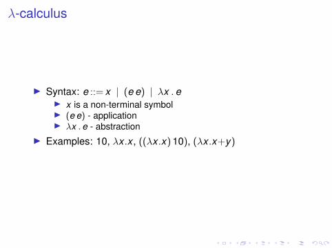
I Syntax: e ::= x | (e e) | λx .eI x is a non-terminal symbolI (e e) - applicationI λx .e - abstraction
I Examples: 10, λx .x , ((λx .x)10), (λx .x+y)
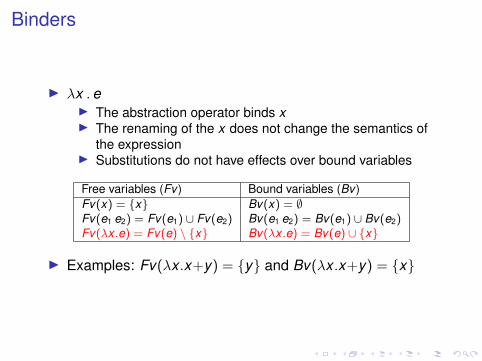
Binders
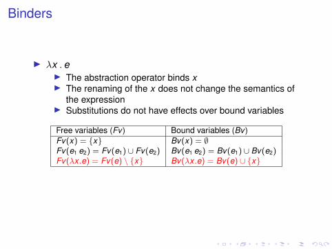
I λx .eI The abstraction operator binds xI The renaming of the x does not change the semantics of
the expressionI Substitutions do not have effects over bound variables
Free variables (Fv ) Bound variables (Bv )Fv(x) = {x} Bv(x) = ∅Fv(e1 e2) = Fv(e1) ∪ Fv(e2) Bv(e1 e2) = Bv(e1) ∪ Bv(e2)Fv(λx .e) = Fv(e) \ {x} Bv(λx .e) = Bv(e) ∪ {x}
I Examples: Fv(λx .x+y) = {y} and Bv(λx .x+y) = {x}
Binders
I λx .eI The abstraction operator binds xI The renaming of the x does not change the semantics of
the expressionI Substitutions do not have effects over bound variables
Free variables (Fv ) Bound variables (Bv )Fv(x) = {x} Bv(x) = ∅Fv(e1 e2) = Fv(e1) ∪ Fv(e2) Bv(e1 e2) = Bv(e1) ∪ Bv(e2)Fv(λx .e) = Fv(e) \ {x} Bv(λx .e) = Bv(e) ∪ {x}
I Examples: Fv(λx .x+y) = {y} and Bv(λx .x+y) = {x}
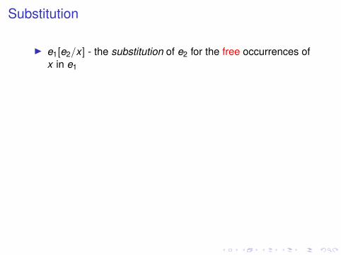
Substitution
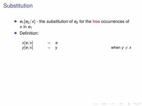
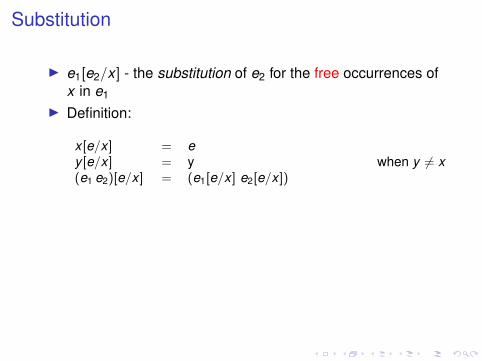
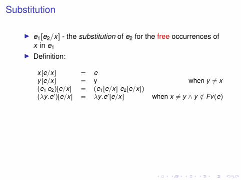
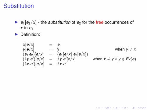
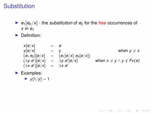
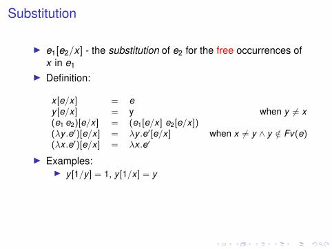
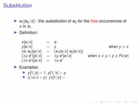
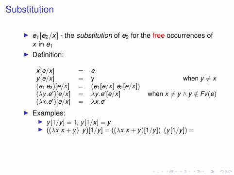
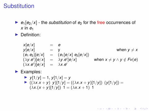
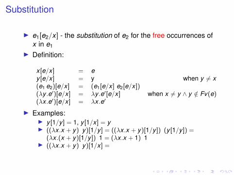
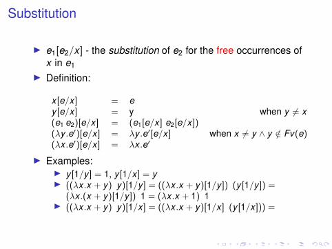
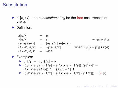
I e1[e2/x ] - the substitution of e2 for the free occurrences ofx in e1
I Definition:
x [e/x ] = ey [e/x ] = y when y 6= x(e1 e2)[e/x ] = (e1[e/x ] e2[e/x ])(λy .e′)[e/x ] = λy .e′[e/x ] when x 6= y ∧ y /∈ Fv(e)(λx .e′)[e/x ] = λx .e′
I Examples:I y [1/y ] = 1, y [1/x ] = yI ((λx .x + y) y)[1/y ] = ((λx .x + y)[1/y ]) (y [1/y ]) =
(λx .(x + y)[1/y ]) 1 = (λx .x + 1) 1I ((λx .x + y) y)[1/x ] = ((λx .x + y)[1/x ] (y [1/x ])) = (? y)
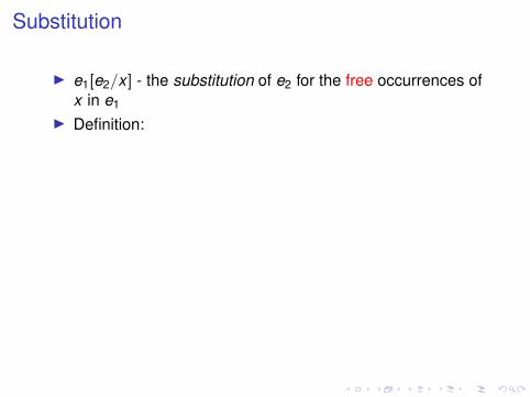
Substitution
I e1[e2/x ] - the substitution of e2 for the free occurrences ofx in e1
I Definition:
x [e/x ] = ey [e/x ] = y when y 6= x(e1 e2)[e/x ] = (e1[e/x ] e2[e/x ])(λy .e′)[e/x ] = λy .e′[e/x ] when x 6= y ∧ y /∈ Fv(e)(λx .e′)[e/x ] = λx .e′
I Examples:I y [1/y ] = 1, y [1/x ] = yI ((λx .x + y) y)[1/y ] = ((λx .x + y)[1/y ]) (y [1/y ]) =
(λx .(x + y)[1/y ]) 1 = (λx .x + 1) 1I ((λx .x + y) y)[1/x ] = ((λx .x + y)[1/x ] (y [1/x ])) = (? y)
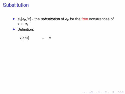
Substitution
I e1[e2/x ] - the substitution of e2 for the free occurrences ofx in e1
I Definition:
x [e/x ] = e
y [e/x ] = y when y 6= x(e1 e2)[e/x ] = (e1[e/x ] e2[e/x ])(λy .e′)[e/x ] = λy .e′[e/x ] when x 6= y ∧ y /∈ Fv(e)(λx .e′)[e/x ] = λx .e′
I Examples:I y [1/y ] = 1, y [1/x ] = yI ((λx .x + y) y)[1/y ] = ((λx .x + y)[1/y ]) (y [1/y ]) =
(λx .(x + y)[1/y ]) 1 = (λx .x + 1) 1I ((λx .x + y) y)[1/x ] = ((λx .x + y)[1/x ] (y [1/x ])) = (? y)
Substitution
I e1[e2/x ] - the substitution of e2 for the free occurrences ofx in e1
I Definition:
x [e/x ] = ey [e/x ] = y when y 6= x
(e1 e2)[e/x ] = (e1[e/x ] e2[e/x ])(λy .e′)[e/x ] = λy .e′[e/x ] when x 6= y ∧ y /∈ Fv(e)(λx .e′)[e/x ] = λx .e′
I Examples:I y [1/y ] = 1, y [1/x ] = yI ((λx .x + y) y)[1/y ] = ((λx .x + y)[1/y ]) (y [1/y ]) =
(λx .(x + y)[1/y ]) 1 = (λx .x + 1) 1I ((λx .x + y) y)[1/x ] = ((λx .x + y)[1/x ] (y [1/x ])) = (? y)
Substitution
I e1[e2/x ] - the substitution of e2 for the free occurrences ofx in e1
I Definition:
x [e/x ] = ey [e/x ] = y when y 6= x(e1 e2)[e/x ] = (e1[e/x ] e2[e/x ])
(λy .e′)[e/x ] = λy .e′[e/x ] when x 6= y ∧ y /∈ Fv(e)(λx .e′)[e/x ] = λx .e′
I Examples:I y [1/y ] = 1, y [1/x ] = yI ((λx .x + y) y)[1/y ] = ((λx .x + y)[1/y ]) (y [1/y ]) =
(λx .(x + y)[1/y ]) 1 = (λx .x + 1) 1I ((λx .x + y) y)[1/x ] = ((λx .x + y)[1/x ] (y [1/x ])) = (? y)
Substitution
I e1[e2/x ] - the substitution of e2 for the free occurrences ofx in e1
I Definition:
x [e/x ] = ey [e/x ] = y when y 6= x(e1 e2)[e/x ] = (e1[e/x ] e2[e/x ])(λy .e′)[e/x ] = λy .e′[e/x ] when x 6= y ∧ y /∈ Fv(e)
(λx .e′)[e/x ] = λx .e′
I Examples:I y [1/y ] = 1, y [1/x ] = yI ((λx .x + y) y)[1/y ] = ((λx .x + y)[1/y ]) (y [1/y ]) =
(λx .(x + y)[1/y ]) 1 = (λx .x + 1) 1I ((λx .x + y) y)[1/x ] = ((λx .x + y)[1/x ] (y [1/x ])) = (? y)
Substitution
I e1[e2/x ] - the substitution of e2 for the free occurrences ofx in e1
I Definition:
x [e/x ] = ey [e/x ] = y when y 6= x(e1 e2)[e/x ] = (e1[e/x ] e2[e/x ])(λy .e′)[e/x ] = λy .e′[e/x ] when x 6= y ∧ y /∈ Fv(e)(λx .e′)[e/x ] = λx .e′
I Examples:I y [1/y ] = 1, y [1/x ] = yI ((λx .x + y) y)[1/y ] = ((λx .x + y)[1/y ]) (y [1/y ]) =
(λx .(x + y)[1/y ]) 1 = (λx .x + 1) 1I ((λx .x + y) y)[1/x ] = ((λx .x + y)[1/x ] (y [1/x ])) = (? y)
Substitution
I e1[e2/x ] - the substitution of e2 for the free occurrences ofx in e1
I Definition:
x [e/x ] = ey [e/x ] = y when y 6= x(e1 e2)[e/x ] = (e1[e/x ] e2[e/x ])(λy .e′)[e/x ] = λy .e′[e/x ] when x 6= y ∧ y /∈ Fv(e)(λx .e′)[e/x ] = λx .e′
I Examples:I y [1/y ] = 1
, y [1/x ] = yI ((λx .x + y) y)[1/y ] = ((λx .x + y)[1/y ]) (y [1/y ]) =
(λx .(x + y)[1/y ]) 1 = (λx .x + 1) 1I ((λx .x + y) y)[1/x ] = ((λx .x + y)[1/x ] (y [1/x ])) = (? y)
Substitution
I e1[e2/x ] - the substitution of e2 for the free occurrences ofx in e1
I Definition:
x [e/x ] = ey [e/x ] = y when y 6= x(e1 e2)[e/x ] = (e1[e/x ] e2[e/x ])(λy .e′)[e/x ] = λy .e′[e/x ] when x 6= y ∧ y /∈ Fv(e)(λx .e′)[e/x ] = λx .e′
I Examples:I y [1/y ] = 1, y [1/x ] = y
I ((λx .x + y) y)[1/y ] = ((λx .x + y)[1/y ]) (y [1/y ]) =(λx .(x + y)[1/y ]) 1 = (λx .x + 1) 1
I ((λx .x + y) y)[1/x ] = ((λx .x + y)[1/x ] (y [1/x ])) = (? y)
Substitution
I e1[e2/x ] - the substitution of e2 for the free occurrences ofx in e1
I Definition:
x [e/x ] = ey [e/x ] = y when y 6= x(e1 e2)[e/x ] = (e1[e/x ] e2[e/x ])(λy .e′)[e/x ] = λy .e′[e/x ] when x 6= y ∧ y /∈ Fv(e)(λx .e′)[e/x ] = λx .e′
I Examples:I y [1/y ] = 1, y [1/x ] = yI ((λx .x + y) y)[1/y ] =
((λx .x + y)[1/y ]) (y [1/y ]) =(λx .(x + y)[1/y ]) 1 = (λx .x + 1) 1
I ((λx .x + y) y)[1/x ] = ((λx .x + y)[1/x ] (y [1/x ])) = (? y)
Substitution
I e1[e2/x ] - the substitution of e2 for the free occurrences ofx in e1
I Definition:
x [e/x ] = ey [e/x ] = y when y 6= x(e1 e2)[e/x ] = (e1[e/x ] e2[e/x ])(λy .e′)[e/x ] = λy .e′[e/x ] when x 6= y ∧ y /∈ Fv(e)(λx .e′)[e/x ] = λx .e′
I Examples:I y [1/y ] = 1, y [1/x ] = yI ((λx .x + y) y)[1/y ] = ((λx .x + y)[1/y ]) (y [1/y ]) =
(λx .(x + y)[1/y ]) 1 = (λx .x + 1) 1I ((λx .x + y) y)[1/x ] = ((λx .x + y)[1/x ] (y [1/x ])) = (? y)

Substitution
I e1[e2/x ] - the substitution of e2 for the free occurrences ofx in e1
I Definition:
x [e/x ] = ey [e/x ] = y when y 6= x(e1 e2)[e/x ] = (e1[e/x ] e2[e/x ])(λy .e′)[e/x ] = λy .e′[e/x ] when x 6= y ∧ y /∈ Fv(e)(λx .e′)[e/x ] = λx .e′
I Examples:I y [1/y ] = 1, y [1/x ] = yI ((λx .x + y) y)[1/y ] = ((λx .x + y)[1/y ]) (y [1/y ]) =
(λx .(x + y)[1/y ]) 1 =
(λx .x + 1) 1I ((λx .x + y) y)[1/x ] = ((λx .x + y)[1/x ] (y [1/x ])) = (? y)
Substitution
I e1[e2/x ] - the substitution of e2 for the free occurrences ofx in e1
I Definition:
x [e/x ] = ey [e/x ] = y when y 6= x(e1 e2)[e/x ] = (e1[e/x ] e2[e/x ])(λy .e′)[e/x ] = λy .e′[e/x ] when x 6= y ∧ y /∈ Fv(e)(λx .e′)[e/x ] = λx .e′
I Examples:I y [1/y ] = 1, y [1/x ] = yI ((λx .x + y) y)[1/y ] = ((λx .x + y)[1/y ]) (y [1/y ]) =
(λx .(x + y)[1/y ]) 1 = (λx .x + 1) 1
I ((λx .x + y) y)[1/x ] = ((λx .x + y)[1/x ] (y [1/x ])) = (? y)
Substitution
I e1[e2/x ] - the substitution of e2 for the free occurrences ofx in e1
I Definition:
x [e/x ] = ey [e/x ] = y when y 6= x(e1 e2)[e/x ] = (e1[e/x ] e2[e/x ])(λy .e′)[e/x ] = λy .e′[e/x ] when x 6= y ∧ y /∈ Fv(e)(λx .e′)[e/x ] = λx .e′
I Examples:I y [1/y ] = 1, y [1/x ] = yI ((λx .x + y) y)[1/y ] = ((λx .x + y)[1/y ]) (y [1/y ]) =
(λx .(x + y)[1/y ]) 1 = (λx .x + 1) 1I ((λx .x + y) y)[1/x ] =
((λx .x + y)[1/x ] (y [1/x ])) = (? y)
Substitution
I e1[e2/x ] - the substitution of e2 for the free occurrences ofx in e1
I Definition:
x [e/x ] = ey [e/x ] = y when y 6= x(e1 e2)[e/x ] = (e1[e/x ] e2[e/x ])(λy .e′)[e/x ] = λy .e′[e/x ] when x 6= y ∧ y /∈ Fv(e)(λx .e′)[e/x ] = λx .e′
I Examples:I y [1/y ] = 1, y [1/x ] = yI ((λx .x + y) y)[1/y ] = ((λx .x + y)[1/y ]) (y [1/y ]) =
(λx .(x + y)[1/y ]) 1 = (λx .x + 1) 1I ((λx .x + y) y)[1/x ] = ((λx .x + y)[1/x ] (y [1/x ])) =
(? y)
Substitution
I e1[e2/x ] - the substitution of e2 for the free occurrences ofx in e1
I Definition:
x [e/x ] = ey [e/x ] = y when y 6= x(e1 e2)[e/x ] = (e1[e/x ] e2[e/x ])(λy .e′)[e/x ] = λy .e′[e/x ] when x 6= y ∧ y /∈ Fv(e)(λx .e′)[e/x ] = λx .e′
I Examples:I y [1/y ] = 1, y [1/x ] = yI ((λx .x + y) y)[1/y ] = ((λx .x + y)[1/y ]) (y [1/y ]) =
(λx .(x + y)[1/y ]) 1 = (λx .x + 1) 1I ((λx .x + y) y)[1/x ] = ((λx .x + y)[1/x ] (y [1/x ])) = (? y)
Alpha - equivalence
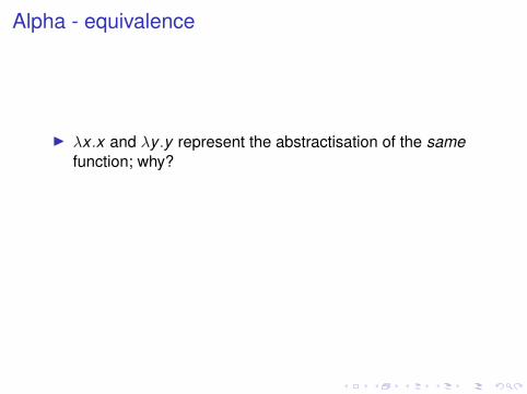
I λx .x and λy .y represent the abstractisation of the samefunction; why?
I α− equivalence:λx .e ≡α λy .e[y/x ], where y is fresh (6∈ Fv(e))
I Example: (λx .x + y) ≡α (λz.(x + y)[z/x ]) = (λz.z + y)
Alpha - equivalence
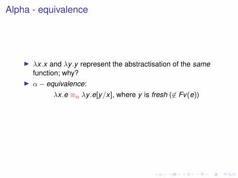
I λx .x and λy .y represent the abstractisation of the samefunction; why?
I α− equivalence:λx .e ≡α λy .e[y/x ], where y is fresh (6∈ Fv(e))
I Example: (λx .x + y) ≡α (λz.(x + y)[z/x ]) = (λz.z + y)
Alpha - equivalence
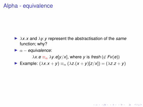
I λx .x and λy .y represent the abstractisation of the samefunction; why?
I α− equivalence:λx .e ≡α λy .e[y/x ], where y is fresh (6∈ Fv(e))
I Example: (λx .x + y) ≡α (λz.(x + y)[z/x ]) = (λz.z + y)
Beta - reduction
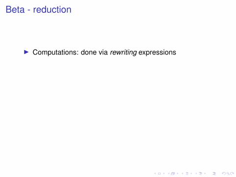
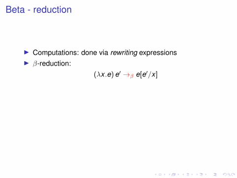
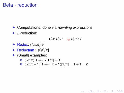
I Computations: done via rewriting expressions
I β-reduction:(λx .e)e′ →β e[e′/x ]
I Redex: (λx .e)e′
I Reductum : e[e′/x ]I (Small) examples:
I (λx .x) 1→β x [1/x ] = 1I (λx .x + 1) 1→β (x + 1)[1/x ] = 1 + 1 = 2
Beta - reduction
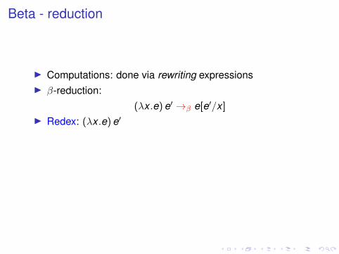
I Computations: done via rewriting expressionsI β-reduction:
(λx .e)e′ →β e[e′/x ]
I Redex: (λx .e)e′
I Reductum : e[e′/x ]I (Small) examples:
I (λx .x) 1→β x [1/x ] = 1I (λx .x + 1) 1→β (x + 1)[1/x ] = 1 + 1 = 2
Beta - reduction
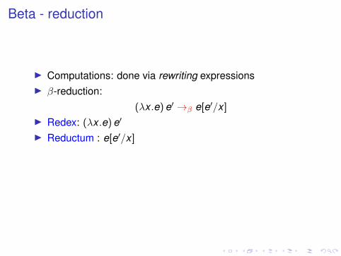
I Computations: done via rewriting expressionsI β-reduction:
(λx .e)e′ →β e[e′/x ]I Redex: (λx .e)e′
I Reductum : e[e′/x ]I (Small) examples:
I (λx .x) 1→β x [1/x ] = 1I (λx .x + 1) 1→β (x + 1)[1/x ] = 1 + 1 = 2
Beta - reduction
I Computations: done via rewriting expressionsI β-reduction:
(λx .e)e′ →β e[e′/x ]I Redex: (λx .e)e′
I Reductum : e[e′/x ]
I (Small) examples:I (λx .x) 1→β x [1/x ] = 1I (λx .x + 1) 1→β (x + 1)[1/x ] = 1 + 1 = 2
Beta - reduction
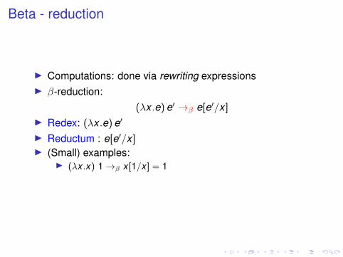
I Computations: done via rewriting expressionsI β-reduction:
(λx .e)e′ →β e[e′/x ]I Redex: (λx .e)e′
I Reductum : e[e′/x ]I (Small) examples:
I (λx .x) 1→β x [1/x ] = 1
I (λx .x + 1) 1→β (x + 1)[1/x ] = 1 + 1 = 2
Beta - reduction
I Computations: done via rewriting expressionsI β-reduction:
(λx .e)e′ →β e[e′/x ]I Redex: (λx .e)e′
I Reductum : e[e′/x ]I (Small) examples:
I (λx .x) 1→β x [1/x ] = 1I (λx .x + 1) 1→β (x + 1)[1/x ] = 1 + 1 = 2
Normal forms
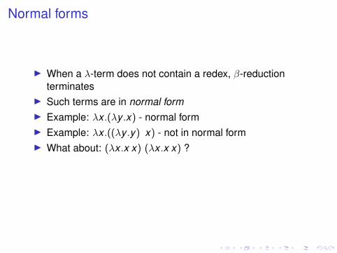
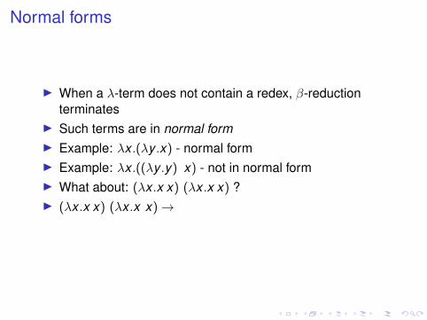
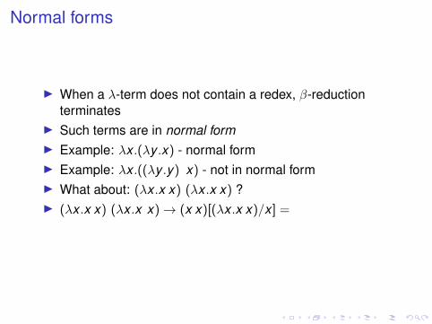
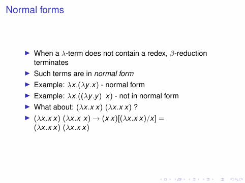
I When a λ-term does not contain a redex, β-reductionterminates
I Such terms are in normal formI Example: λx .(λy .x) - normal formI Example: λx .((λy .y) x) - not in normal formI What about: (λx .x x) (λx .x x) ?I (λx .x x) (λx .x x)→ (x x)[(λx .x x)/x ] =
(λx .x x) (λx .x x)→ · · ·
Normal forms
I When a λ-term does not contain a redex, β-reductionterminates
I Such terms are in normal form
I Example: λx .(λy .x) - normal formI Example: λx .((λy .y) x) - not in normal formI What about: (λx .x x) (λx .x x) ?I (λx .x x) (λx .x x)→ (x x)[(λx .x x)/x ] =
(λx .x x) (λx .x x)→ · · ·
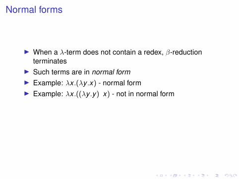
Normal forms
I When a λ-term does not contain a redex, β-reductionterminates
I Such terms are in normal formI Example: λx .(λy .x) - normal formI Example: λx .((λy .y) x) - not in normal form
I What about: (λx .x x) (λx .x x) ?I (λx .x x) (λx .x x)→ (x x)[(λx .x x)/x ] =
(λx .x x) (λx .x x)→ · · ·
Normal forms
I When a λ-term does not contain a redex, β-reductionterminates
I Such terms are in normal formI Example: λx .(λy .x) - normal formI Example: λx .((λy .y) x) - not in normal formI What about: (λx .x x) (λx .x x) ?
I (λx .x x) (λx .x x)→ (x x)[(λx .x x)/x ] =(λx .x x) (λx .x x)→ · · ·
Normal forms
I When a λ-term does not contain a redex, β-reductionterminates
I Such terms are in normal formI Example: λx .(λy .x) - normal formI Example: λx .((λy .y) x) - not in normal formI What about: (λx .x x) (λx .x x) ?I (λx .x x) (λx .x x)→
(x x)[(λx .x x)/x ] =(λx .x x) (λx .x x)→ · · ·
Normal forms
I When a λ-term does not contain a redex, β-reductionterminates
I Such terms are in normal formI Example: λx .(λy .x) - normal formI Example: λx .((λy .y) x) - not in normal formI What about: (λx .x x) (λx .x x) ?I (λx .x x) (λx .x x)→ (x x)[(λx .x x)/x ] =
(λx .x x) (λx .x x)→ · · ·
Normal forms
I When a λ-term does not contain a redex, β-reductionterminates
I Such terms are in normal formI Example: λx .(λy .x) - normal formI Example: λx .((λy .y) x) - not in normal formI What about: (λx .x x) (λx .x x) ?I (λx .x x) (λx .x x)→ (x x)[(λx .x x)/x ] =
(λx .x x) (λx .x x)
→ · · ·

Normal forms
I When a λ-term does not contain a redex, β-reductionterminates
I Such terms are in normal formI Example: λx .(λy .x) - normal formI Example: λx .((λy .y) x) - not in normal formI What about: (λx .x x) (λx .x x) ?I (λx .x x) (λx .x x)→ (x x)[(λx .x x)/x ] =
(λx .x x) (λx .x x)→ · · ·
Recursion
I How to define recursive functions?
I Example:
sum∆= λn.if (n ≤ 0)then0elsen + (sum(n − 1))
I Let’s do it in Haskell!
Recursion
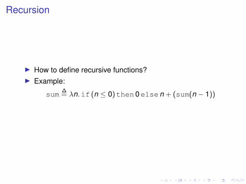
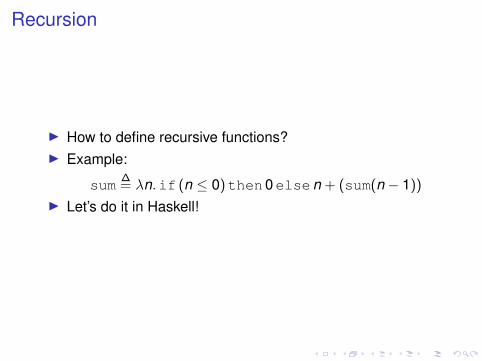
I How to define recursive functions?I Example:
sum∆= λn.if (n ≤ 0)then0elsen + (sum(n − 1))
I Let’s do it in Haskell!
Recursion
I How to define recursive functions?I Example:
sum∆= λn.if (n ≤ 0)then0elsen + (sum(n − 1))
I Let’s do it in Haskell!
Haskell example explained
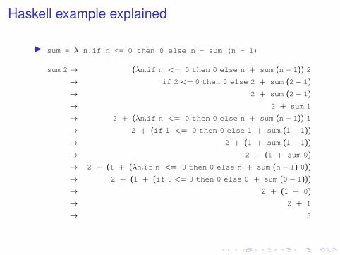
I sum = λ n.if n <= 0 then 0 else n + sum (n - 1)
sum 2→ (λn.if n <= 0 then 0 else n + sum (n− 1)) 2
→ if 2 <= 0 then 0 else 2 + sum (2− 1)
→ 2 + sum (2− 1)
→ 2 + sum 1
→ 2 + (λn.if n <= 0 then 0 else n + sum (n− 1)) 1
→ 2 + (if 1 <= 0 then 0 else 1 + sum (1− 1))
→ 2 + (1 + sum (1− 1))
→ 2 + (1 + sum 0)
→ 2 + (1 + (λn.if n <= 0 then 0 else n + sum (n− 1) 0))
→ 2 + (1 + (if 0 <= 0 then 0 else 0 + sum (0− 1)))
→ 2 + (1 + 0)
→ 2 + 1
→ 3
The Y-combinator
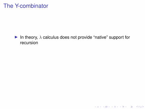
I In theory, λ calculus does not provide “native” support forrecursion
I But, it is possible to add it using the Y -combinatorI Combinators are λ expressions without free variables
I The Y-combinator:λf .(λx .f (x x)) (λx .f (x x))
The Y-combinator
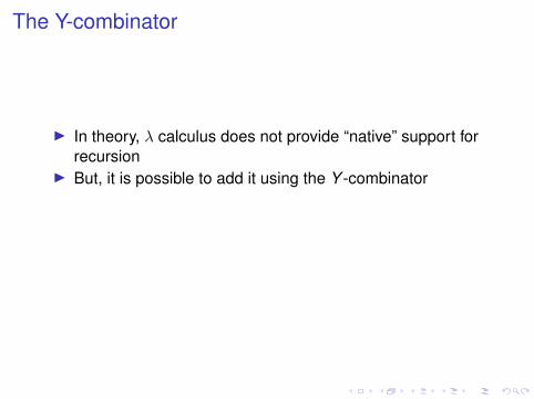
I In theory, λ calculus does not provide “native” support forrecursion
I But, it is possible to add it using the Y -combinator
I Combinators are λ expressions without free variablesI The Y-combinator:
λf .(λx .f (x x)) (λx .f (x x))
The Y-combinator
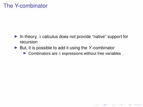
I In theory, λ calculus does not provide “native” support forrecursion
I But, it is possible to add it using the Y -combinatorI Combinators are λ expressions without free variables
I The Y-combinator:λf .(λx .f (x x)) (λx .f (x x))
The Y-combinator
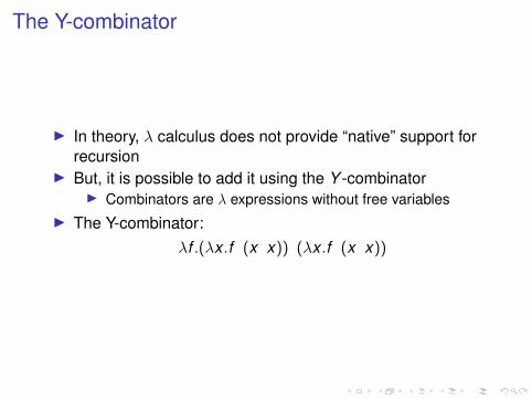
I In theory, λ calculus does not provide “native” support forrecursion
I But, it is possible to add it using the Y -combinatorI Combinators are λ expressions without free variables
I The Y-combinator:λf .(λx .f (x x)) (λx .f (x x))
Evaluation
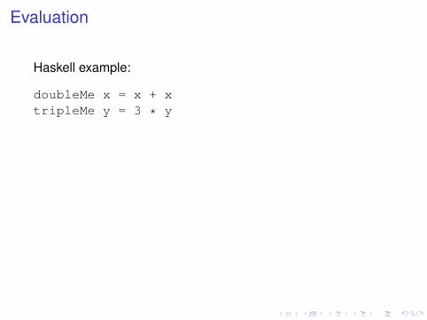
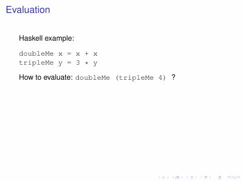
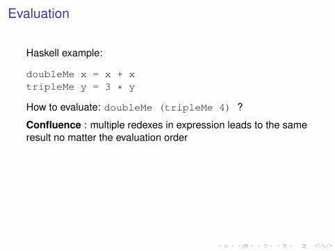
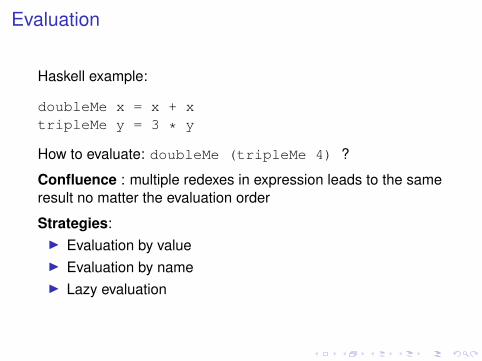
Haskell example:
doubleMe x = x + xtripleMe y = 3 * y
How to evaluate: doubleMe (tripleMe 4) ?
Confluence : multiple redexes in expression leads to the sameresult no matter the evaluation order
Strategies:I Evaluation by valueI Evaluation by nameI Lazy evaluation
Evaluation
Haskell example:
doubleMe x = x + xtripleMe y = 3 * y
How to evaluate: doubleMe (tripleMe 4) ?
Confluence : multiple redexes in expression leads to the sameresult no matter the evaluation order
Strategies:I Evaluation by valueI Evaluation by nameI Lazy evaluation
Evaluation
Haskell example:
doubleMe x = x + xtripleMe y = 3 * y
How to evaluate: doubleMe (tripleMe 4) ?
Confluence : multiple redexes in expression leads to the sameresult no matter the evaluation order
Strategies:I Evaluation by valueI Evaluation by nameI Lazy evaluation
Evaluation
Haskell example:
doubleMe x = x + xtripleMe y = 3 * y
How to evaluate: doubleMe (tripleMe 4) ?
Confluence : multiple redexes in expression leads to the sameresult no matter the evaluation order
Strategies:I Evaluation by valueI Evaluation by nameI Lazy evaluation
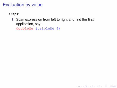
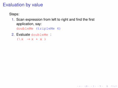
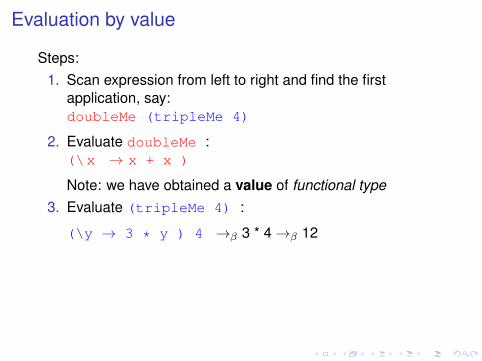
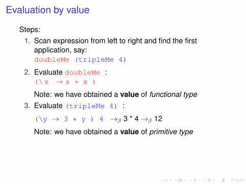
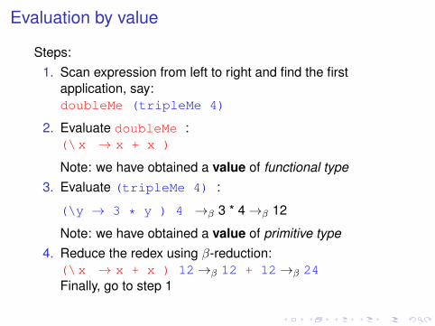
Evaluation by value
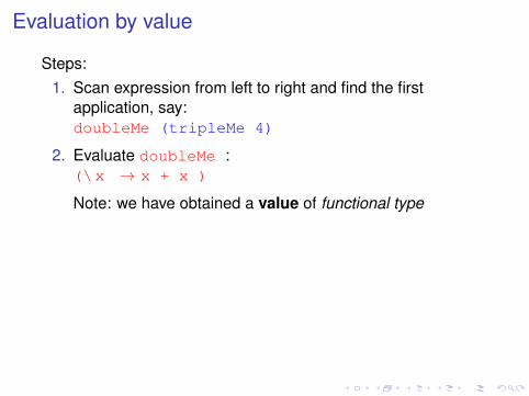
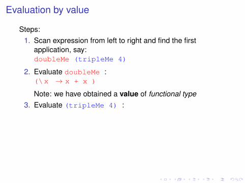
Steps:1. Scan expression from left to right and find the first
application, say:doubleMe (tripleMe 4)
2. Evaluate doubleMe :(\x → x + x )
Note: we have obtained a value of functional type3. Evaluate (tripleMe 4) :
(\y → 3 * y ) 4 →β 3 * 4→β 12
Note: we have obtained a value of primitive type4. Reduce the redex using β-reduction:
(\x → x + x ) 12→β 12 + 12→β 24Finally, go to step 1
Evaluation by value
Steps:1. Scan expression from left to right and find the first
application, say:doubleMe (tripleMe 4)
2. Evaluate doubleMe :(\x → x + x )
Note: we have obtained a value of functional type
3. Evaluate (tripleMe 4) :
(\y → 3 * y ) 4 →β 3 * 4→β 12
Note: we have obtained a value of primitive type4. Reduce the redex using β-reduction:
(\x → x + x ) 12→β 12 + 12→β 24Finally, go to step 1
Evaluation by value
Steps:1. Scan expression from left to right and find the first
application, say:doubleMe (tripleMe 4)
2. Evaluate doubleMe :(\x → x + x )
Note: we have obtained a value of functional type3. Evaluate (tripleMe 4) :
(\y → 3 * y ) 4 →β 3 * 4→β 12
Note: we have obtained a value of primitive type4. Reduce the redex using β-reduction:
(\x → x + x ) 12→β 12 + 12→β 24Finally, go to step 1
Evaluation by value
Steps:1. Scan expression from left to right and find the first
application, say:doubleMe (tripleMe 4)
2. Evaluate doubleMe :(\x → x + x )
Note: we have obtained a value of functional type3. Evaluate (tripleMe 4) :
(\y → 3 * y ) 4 →β 3 * 4→β 12
Note: we have obtained a value of primitive type
4. Reduce the redex using β-reduction:(\x → x + x ) 12→β 12 + 12→β 24Finally, go to step 1
Evaluation by value
Steps:1. Scan expression from left to right and find the first
application, say:doubleMe (tripleMe 4)
2. Evaluate doubleMe :(\x → x + x )
Note: we have obtained a value of functional type3. Evaluate (tripleMe 4) :
(\y → 3 * y ) 4 →β 3 * 4→β 12
Note: we have obtained a value of primitive type4. Reduce the redex using β-reduction:
(\x → x + x ) 12→β 12 + 12→β 24Finally, go to step 1
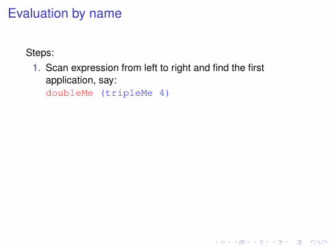
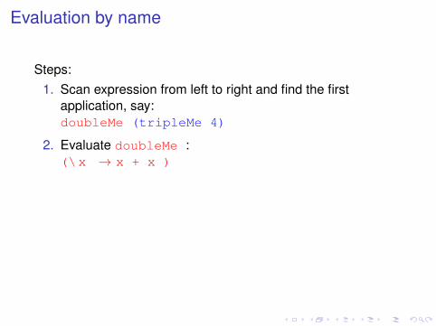
Evaluation by name
Steps:1. Scan expression from left to right and find the first
application, say:doubleMe (tripleMe 4)
2. Evaluate doubleMe :(\x → x + x )
Note: we have obtained a value of functional type3. Reduce the redex using β-reduction:
(\x → x + x ) tripleMe 4→β
(tripleMe 4) + (tripleMe 4)→β · · · →β 24
Finally, go to step 1
Evaluation by name
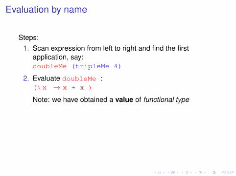
Steps:1. Scan expression from left to right and find the first
application, say:doubleMe (tripleMe 4)
2. Evaluate doubleMe :(\x → x + x )
Note: we have obtained a value of functional type
3. Reduce the redex using β-reduction:(\x → x + x ) tripleMe 4→β
(tripleMe 4) + (tripleMe 4)→β · · · →β 24
Finally, go to step 1

Evaluation by name
Steps:1. Scan expression from left to right and find the first
application, say:doubleMe (tripleMe 4)
2. Evaluate doubleMe :(\x → x + x )
Note: we have obtained a value of functional type3. Reduce the redex using β-reduction:
(\x → x + x ) tripleMe 4→β
(tripleMe 4) + (tripleMe 4)→β · · · →β 24
Finally, go to step 1
Lazy evaluation
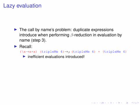
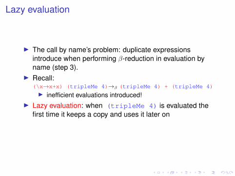
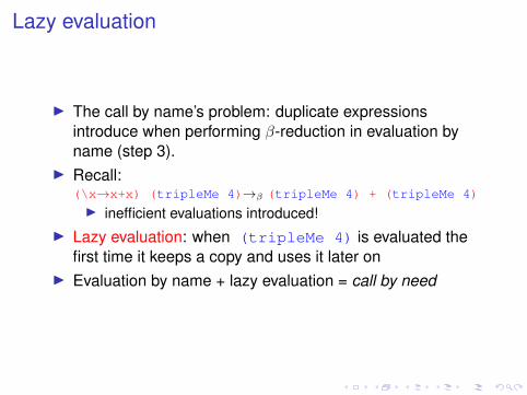
I The call by name’s problem: duplicate expressionsintroduce when performing β-reduction in evaluation byname (step 3).
I Recall:(\x→x+x) (tripleMe 4)→β (tripleMe 4) + (tripleMe 4)
I inefficient evaluations introduced!I Lazy evaluation: when (tripleMe 4) is evaluated the
first time it keeps a copy and uses it later onI Evaluation by name + lazy evaluation = call by need

Lazy evaluation
I The call by name’s problem: duplicate expressionsintroduce when performing β-reduction in evaluation byname (step 3).
I Recall:(\x→x+x) (tripleMe 4)→β (tripleMe 4) + (tripleMe 4)
I inefficient evaluations introduced!I Lazy evaluation: when (tripleMe 4) is evaluated the
first time it keeps a copy and uses it later onI Evaluation by name + lazy evaluation = call by need
Lazy evaluation
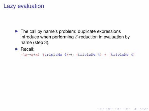
I The call by name’s problem: duplicate expressionsintroduce when performing β-reduction in evaluation byname (step 3).
I Recall:(\x→x+x) (tripleMe 4)→β (tripleMe 4) + (tripleMe 4)
I inefficient evaluations introduced!
I Lazy evaluation: when (tripleMe 4) is evaluated thefirst time it keeps a copy and uses it later on
I Evaluation by name + lazy evaluation = call by need
Lazy evaluation
I The call by name’s problem: duplicate expressionsintroduce when performing β-reduction in evaluation byname (step 3).
I Recall:(\x→x+x) (tripleMe 4)→β (tripleMe 4) + (tripleMe 4)
I inefficient evaluations introduced!I Lazy evaluation: when (tripleMe 4) is evaluated the
first time it keeps a copy and uses it later on
I Evaluation by name + lazy evaluation = call by need
Lazy evaluation
I The call by name’s problem: duplicate expressionsintroduce when performing β-reduction in evaluation byname (step 3).
I Recall:(\x→x+x) (tripleMe 4)→β (tripleMe 4) + (tripleMe 4)
I inefficient evaluations introduced!I Lazy evaluation: when (tripleMe 4) is evaluated the
first time it keeps a copy and uses it later onI Evaluation by name + lazy evaluation = call by need
Functional programming in Haskell
I Integers, BooleansI TypesI Lists: head, tail, reverse, reverse, sum, infinite listsI Lazy evaluation: examples using functions on infinite listsI Higher-order functions: map, foldlI Generate prime numbers
Resources
Please refer to the book:I Chapter 11: http://websrv.dthu.edu.vn/
attachments/newsevents/content2415/Programming_Languages_-_Principles_and_Paradigms_thereds1106.pdf
in order to grasp other related items:1. local environment2. types3. pattern matching4. infinite objects