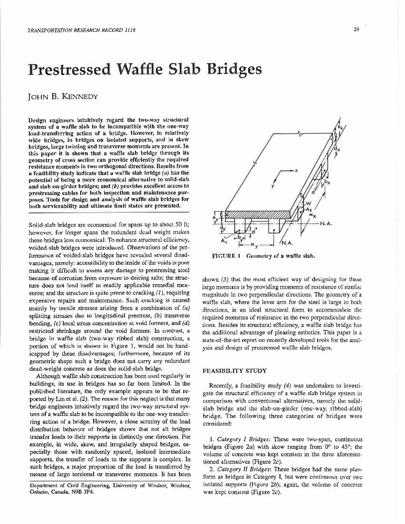
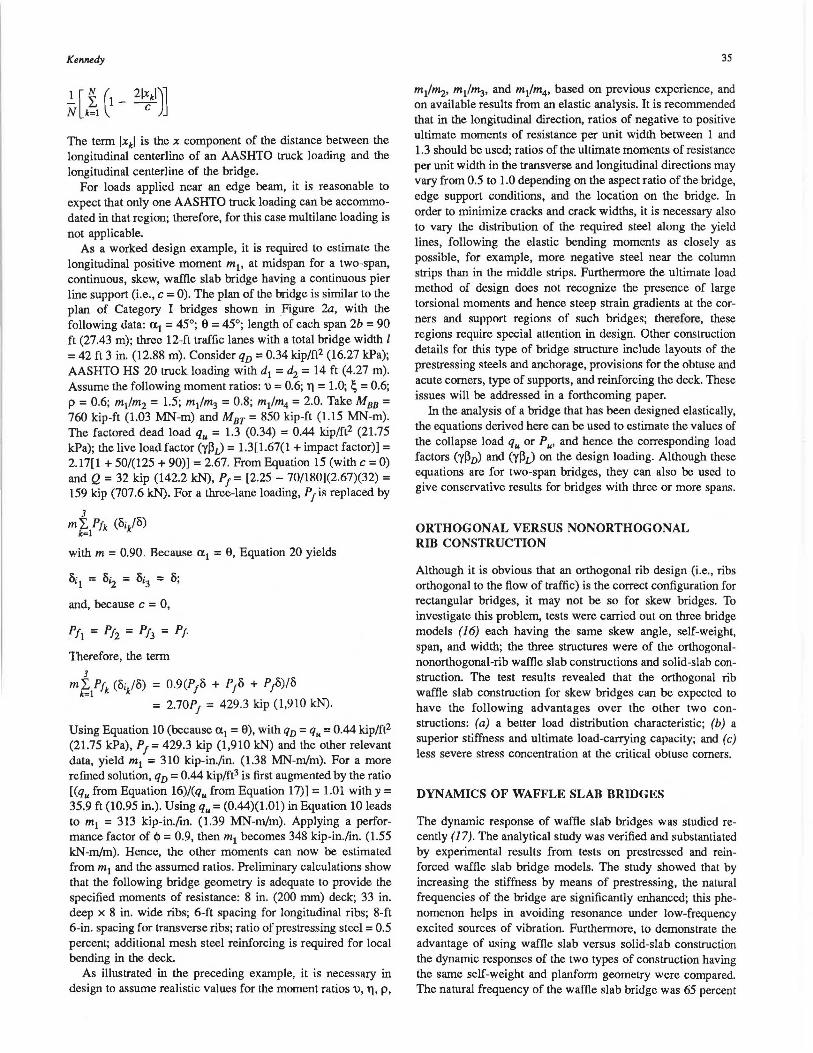
TRANSPORTATION RESEARCH RECORD 1118 29

Prestressed Waffle Slab Bridges

JOHN B. KENNEDY

Design engineers Intuitively regard the two-way structural system of a waffle slab to be Incompatible with the one-way load-transferring action of a bridge. However, in relatively wide bridges, In bridges on Isolated supports, and in skew bridges, large twisting and transverse moments are present. !n this paper it Is shown that a waffle slab bridge through its geometry of cross section can provide efficiently the required resistance moments in two orthogonal directions. Results from a feasibility study indicate that a waffle slab bridge (a) has the potential of being a more economical alternative to solid-slab and slab-on-girder bridges; and (b) provides excellent access to prestresslng cables for both inspection and maintenance pur­poses. Tools for design and analysis of waffle slab bridges for both serviceability and ultimate limit states are presented.

Solid-slab bridges are economical for spans up to about 50 ft; however, for longer spans the redundant dead weight makes these bridges less economical. To enhance structural efficiency, voided-slab bridges were introduced. Observations of the per­formance of voided-slab bridges have revealed several disad­vantages, namely: accessibility to the inside of the voids is poor making it difficult to assess any damage to prestressing steel because of corrosion from exposure to deicing salts; the struc­ture does not lend itself to readily applicable remedial mea­sures; and the structure is quite prone to cracking ( 1 ), requiring expensive repairs and maintenance. Such cracking is caused mainly by tensile stresses arising from a combination of (a) splitting stresses due to longitudinal prestress, (b) transverse bending, (c) local stress concentration at void formers, and (d) restricted shrinkage around the void formers. In contrast, a bridge in waffle slab (two-way ribbed slab) construction, a portion of which is shown in Figure 1, would not be hand­icapped by these disadvantages; furthermore, because of its geometric shape such a bridge does not carry any redundant dead-weight concrete as does the solid-slab bridge.

Although waffle slab construction has been used regularly in buildings, its use in bridges has so far been limited. In the published literature, the only example appears to be that re­ported by Lin et al. (2). The reason for this neglect is that many bridge engineers intuitively regard the two-way structural sys­tem of a waffle slab to be incompatible to the one-way transfer­ring action of a bridge. However, a close scrutiny of the load distribution behavior of bridges shows that not all bridges transfer loads to their supports in distinctly one direction. For example, in wide, skew, and irregularly shaped bridges, es­pecially those with randomly spaced, isolated intermediate supports, the transfer of loads to the supports is complex. In such bridges, a major proportion of the load is transferred by means of large torsional or transverse moments. It has been

Department of Civil Engineering, University of Windsor, Windsor, Ontario, Canada, N9B 3P4.

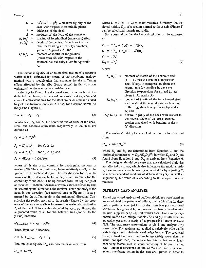
FIGURE 1 Geometry of a waffle slab.

shown (3) that the most efficient way of designing for these large moments is by providing moments of resistance of similaf magnitude in two perpendicular directions. The geometry of a waffle slab, where the lever arm for the steel is large in both directions, is an ideal structural form to accommodate the required moments of resistance in the two perpendicular direc­tions. Besides its structural efficiency, a waffle slab bridge has the additional advantage of pleasing esthetics. This paper is 11

state-of-the-art report on recently developed tools for the anal­ysis and design of prestressed waffle slab bridges.

FEASIBILITY STUDY

Recently, a feasibility study (4) was undertaken to investi­gate the structural efficiency of a waffle slab bridge system in comparison with conventional alternatives, namely the solid­slab bridge and the slab-on-girder (one-way, ribbed-slab) bridge. The following three categories of bridges were considered:

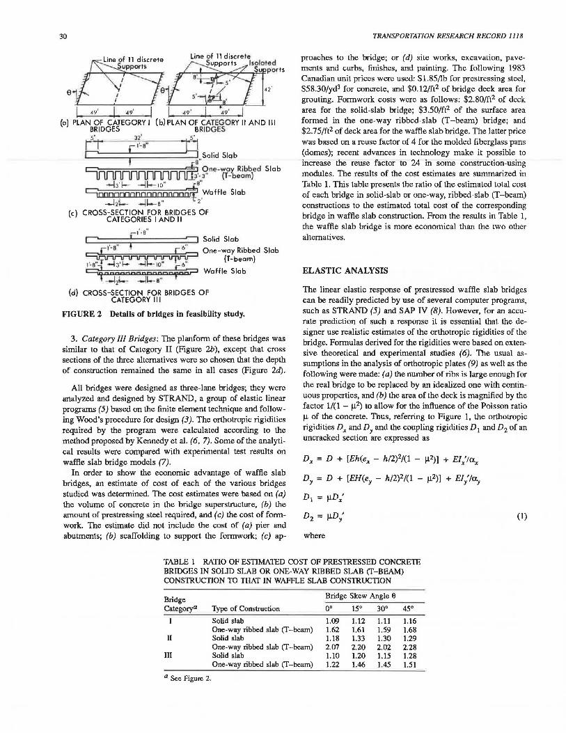
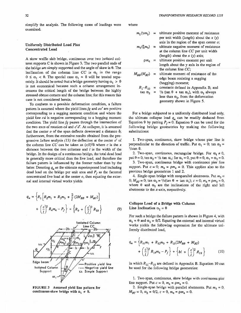
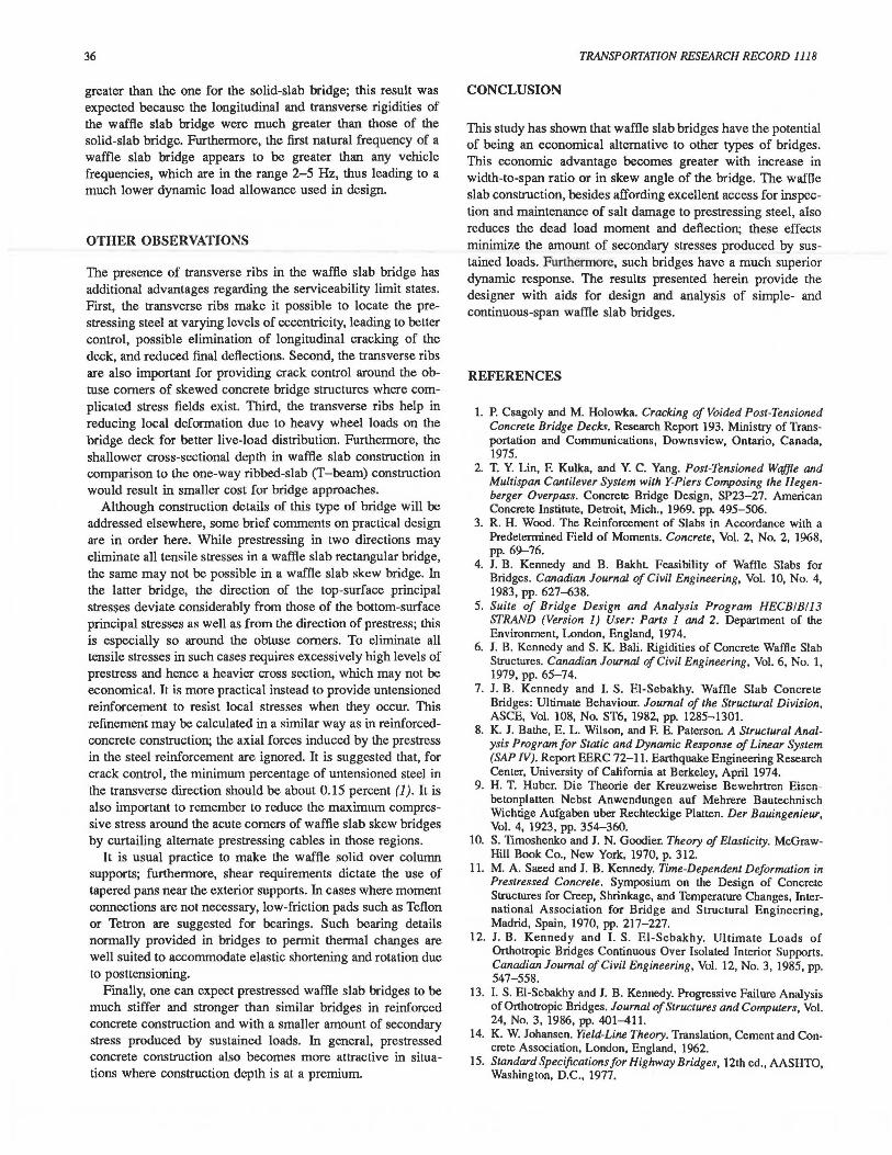
1. Category I Bridges: These were two-span, continuous bridges (Figure 2a) with skew ranging from 0° to 45°; the volume of concrete was kept constant in the three aforemen­tioned alternatives (Figure 2c).

2. Category I/ Bridges: These bridges had the same plan­form as bridges in Category I, but were continuous over two isolated supports (Figure 2b); again, the volume of concrete was kept constant (Figure 2c).

30

a

1 49' 1 49' 1 i.. ~9 · .i . 49 • I (a) PLAN OF CATEGORY I (b)PLAN OF CATEGORY 11 AND Ill

BRIDGES BRIDGES s· :12' s'

P • f i'-a" R Solid Slab a" ~One-way Ribbed Slab ---inrtflflflnf'-3" (T- beam)

- b' I- - H-- 10" ""4e" 9nnnnmnnnonnooon°'f Waffle Slab

--M- -H-s" 2 '

(c) CROSS-SECTION FOR BRIDGES OF CATEGORIES I AND 11

r:1'-s" C , ., f ,;=t Solid Slab ~One-way Ribbed Slab

1·- a·~u.,..r J''t-" u~'l-~o~ u '.:6~ (T-beam)

9 ::17l:'"::lt:·;..n0 f'O? Waffle Slab

(d) CROSS-SECTION FOR BRIDGES OF CATEGORY Ill

FIGURE 2 Details of bridges in feasibility study.

3. Category III Bridges: The planform of these bridges was similar to that of Category II (Figure 2b), except that cross sections of the three alternatives were so chosen that the depth of construction remained the same in all cases (Figure 2<f).

All bridges were designed as three-lane bridges; they were analyzed and designed by STRAND, a group of elastic linear programs (5) based on the finite element technique and follow­ing Wood's procedure for design (3). The orthotropic rigidities required by the program were calculated according to the method proposed by Kennedy ct al. (6, 7). Some of the analyti­cal results were compared with experimental test results on waffle slab bridge models (7).

In order to show the economic advantage of waffle slab bridges, an estimate of cost of each of the various bridges studied was determined. The cost estimates were based on (a) the volume of concrete in the bridge superstructure, (b) the amount of prestressing steel required, and ( c) the cost of form­work. The estimate did not include the cost of (a) pier and abutments; (b) scaffolding to support the formwork; (c) ap-

TRANSPORTATION RESEARCH RECORD 1118

proaches to the bridge; or (d) site works, excavation, pave­ments and curbs, finishes, and painting. The following 1983 Canadian unit prices were used: $1.85/lb for prestressing steel, $58.30/yd3 for concrete, and $0.12/ft2 of bridge deck area for grouting. Formwork costs were as follows: $2.80/ft2 of deck area for the solid-slab bridge; $3.50/ft2 of the surface area formed in the one-way ribbed-slab (T-beam) bridge; and $2.75/ft2 of deck area for the waffle slab bridge. The latter price was based on a reuse factor of 4 for the molded fiberglass pans (domes); recent advances in technology make it possible to increase the reuse factor to 24 in some construction-using modules. The results of the cost estimates are summarized in Table 1. This table presents the ratio of the estimated total cost of each bridge in solid-slab or one-way, ribbed-slab (T-beam) constructions to the estimated total cost of the corresponding bridge in waffle slab construction. From the results in Table 1, the waffle slab bridge is more economical than the two other alternatives.

ELASTIC ANALYSIS

The linear elastic response of prestressed waffle slab bridges can be readily predicted by use of several computer programs, such as STRAND (5) and SAP IV (8). However, for an accu­rate prediction of such a response it is essential that the de­signer use realistic estimates of the orthotropic rigidities of the bridge. Formulas derived for the rigidities were based on exten­sive theoretical and experimental studies (6). The usual as­sumptions in the analysis of orthotropic plates (9) as well as the following were made: (a) the number of ribs is large enough for the real bridge to be replaced by an idealized one with contin­uous properties, and (b) the area of the deck is magnified by the factor 1/(1 - µ2) to allow for the influence of the Poisson ratio µof the concrete. Thus, referring to Figure 1, the orthotropic rigidities D,, and DY and the coupling rigidities D 1 and D2 of an uncracked section are expressed as

D,, = D + [Eh(e,, - h/2)2/(l - µ2)] + EI,,'la,,

Dy = D + [EH(ey - h/2)2/(l - µ2)] + Eiy'lay

D2 = µDy'

where

(1)

TABLE 1 RATIO OF ESTIMATED COST OF PRES1RESSED CONCRETE BRIDGES IN SOLID SLAB OR ONE-WAY RIBBED SLAB (T-BEAM) CONS1RUCTION TO THAT IN WAFFLE SLAB CONS1RUCTION

Bridge Bridge Skew Angle 9

Categorya Type of Construction oo 15° 30° 45°

I Solid slab 1.0'J 1.12 1.11 1.16 One-way ribbed slab (T-beam) 1.62 1.61 1.59 1.68

II Solid slab 1.18 1.33 1.30 1.29 One-way ribbed slab (T-beam) 2.07 2.20 2.02 2.28

III Solid slab 1.10 1.20 1.15 1.28 One-way ribbed slab (T-beam) 1.22 1.46 1.45 1.51

a See Figure 2.

Kennedy

D

h E

ex_. (exy) e_. (ey)

I_.' (ly')

=

= = = =

=

Eh3/12(1 - µ2) = flexural rigidity of the deck with respect to its middle plane; thickness of the deck; modulus of elasticity of the concrete; spacing of longitudinal (transverse) ribs; depth of the neutral plane from the top fiber for bending in the x (y) direction, given in Appendix A; and moment of inertia of longitudinal (transverse) rib with respect to the assumed neutral axis, given in Appendix A.

The torsional rigidity of an uncracked section of a concrete waffle slab is estimated by means of the membrane analogy method with a modification that accounts for the stiffening effect afforded by the ribs (beam stems) in the direction orthogonal to the one under consideration.

Referring to Figure 1 and considering the geometry of the deflected membrane, the torsional constants for deck, stem, and concrete equivalent area for the steel are calculated and added to yield the torsional constant 1. Thus, for a section normal to the y-axis (Figure 1),

(2)

in which 11, 12, and 13, the contributions of areas of the deck, stem, and concrete equivalent, respectively, to the steel, are defined as

1 11 = 2 Ki<Xyh3;

12 = K1dyb/, for dy ~ by;

12 = K1byd/, for by ~ dy; and

13 = 4K1 (n - l)(A,')2/1t (3)

where K1 is the usual constant for rectangular sections in torsion (10). The contribution 13, being relatively small, can be ignored in a practical design. The modification for 11 is by means of the reduction factor of 1/z, which accounts for the continuity of the deck, it being distinct from the top flange of an isolated T-section. Because a waffle slab is stiffened by ribs in two orthogonal directions, the torsional contributionl1 of the deck in one direction (see hatched area in Figure 1) is aug­mented by the stiffening rib in the orthogonal direction. Con­sidering the section normal to the x-axis (Figure 1), the pres­ence of the transverse rib W increases the torsional contribution 18 of the deck S to a value denoted by lcs + W)· Hence, the augmented value of 1 1 for the hatched area (normal to the y-axis) becomes

(4)

Thus, Equation 2 becomes

(5)

The torsional rigidity Dyx can now be calculated from

(6)

31

where G = E/2(1 + µ) = shear modulus. Similarly, the tor­sional rigidity Dxy of a section normal to the x-axis (Figure 1) can be calculated mutatis mutandis.

For a cracked section, the flexural rigidities can be expressed as

D_. = E[/8_. + l,j(l - µ2)]/ex_.

Dy = E[/8y + lc/(1 - µ2)]<Xy

Di = µD_.'

D2 =µDy'

where

= moment of inertia of the concrete and (n - 1) times the area of compression steel, if any, in compression about the neutral axis for bending in the x (y) direction (expressions for I ex and Icy are given in Appendix A);

(7)

= moment of inertia of the transformed steel section about the neutral axis for bending in the x (y) direction, given in Appendix A;and

= flexural rigidity of the deck with respect to the neutral plane of the gross cracked section associated with bending in the x (y) direction.

The torsional rigidity for a cracked section can be calculated from

D = ex(D n )1f2 xy x'-'y (8)

where D,. and Dy are detennined from Equation 7, and the torsional parameter ex = D:r:/(D/J./a. in which D_. and DY are found from Equation 1 and Dxy is derived from Equation 6.

The designer should be aware that the calculated rigidities are affected by creep, which also influences the modular ratio n; these influences can be readily accounted for by adjusting Ee to a time-dependent modulus of deformation ( 11 ), as well as augmenting the value of n according to the adopted code of practice.

ULTIMATE LOAD ANALYSES

The ultimate load analyses of waffle slab bridges were based on assumed yield line patterns of failure; the justification for these failure patterns were (a) test results from two post-tensioned waffle slab bridge models, continuous over two isolated interior column supports (12); (b) test results from five simply sup­ported waffle slab bridge models (7); and (c) results from an extensive parametric study of a progressive failure analysis (13 ). The customary assumptions in yield line analysis (14) were made. The analyses are applied to relatively wide waffle slab bridges with relatively weak edge beams. The predicted collapse load has been found to be invariably lower than the actual collapse load; the reason for this is that some load­enhancing factors such as strain hardening of the prestressing steel, torsional resistance of the waffle slab, and to a lesser extent membrane action in the slab are ignored in order to

32

simplify the analysis. The following cases of loadings were examined.

Uniformly Distributed Load Plus Concentrated Load

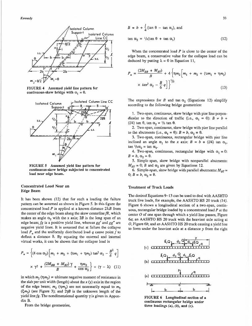
A skew waffle slab bridge, continuous over two isolated col­umn supports C is shown in Figure 3. The two parallel ends of the bridge are simply supported and the angle of skew is 0. The inclination of the column line CC is cx1 in the range 0 ~ cx1 < 0. The special case cx1 = 0 will be treated sepa­rately. It should be noted that a bridge geometry having cx1 > 0 is not economical because such a column arrangement in­creases the critical length of the bridge between the highly stressed obtuse comers and the column line; for this reason this case is not considered herein.

To conform to a possible deformation condition, a failure pattern is assumed where the yield lines Jg and oo' are positive corresponding to a sagging moment condition and where the yield line cd is negative corresponding to a hogging moment condition. The yield line Jg passes through the intersection of the two axes of rotation cd and c' d'. At collapse, it is assumed that the center o of the span deflects downward a distance B; furthermore, from the extensive results obtained from the pro­gressive failure analysis (13) the deflection at the center o' of the column line CC can be taken as (c//)2B where c is the x distance between the two columns and l is the width of the bridge. In the design of a continuous bridge, the total dead load is generally more critical than the live load, and therefore the failure pattern is influenced by the former rather than by the latter. Denoting qu as the ultimate superimposed load including dead load on the bridge per unit area and Pf as the factored concentrated live load at the center o, then equating the exter­nal and internal virtual works yields

qu = {R1 [ Rzm1 + R3"'J + f (2MBB + MBT)J

+ (f )2 R4m4 - Pf} + {R9 + (f )2 Rio}

- Positive yield line --- Negative yield line s:s. Simple Support

FIGURE 3 Assumed yield line pattern for continuous-skew bridge with cx1 -:t- 0.

(9)

TRANSPORTATION RESEARCH RECORD 1118

where

m1 (um1) = ultimate positive moment of resistance

m3(~"'3) =

pm4 -·

MBB(MBT) =

Ri-R10 = tan <Xz =

per unit width (length) about the x (y) axis in the region of the span center o; ultimate negative moment of resistance at the column line CC per unit width (length) about the x (y) axis; ultimate positive moment per unit length about the y axis in the region of the column line CC; ultimate moment of resistance of the edge beam resisting a sagging (hogging) moment; constants defined in Appendix B; and 1/2 (tan 0 + tan cx1), with cx1 always less than exz, from the deformation geometry shown in Figure 5.

For a bridge subjected to a uniformly distributed load only, the ultimate collapse load qu can be readily deduced from Equation 9 by putting Pf= 0. Equation 9 can be used for the following bridge geometries by making the following substitutions:

1. Two-span, continuous, skew bridge whose pier line is perpendicular to the direction of traffic. Put cx1 = O; tan <Xz = 1/ztan 0.

2. Two-span, continuous, rectangular bridge. For cx1 -:f. 0, put 0 = 0, tan <Xz = 1/2 tan cx1; for cx1 = 0, put 0 = 0, cx1 = <Xz = 0.

3. Two-span, continuous bridge with continuous pier line support. Put c = O; m4 = pm4 = 0. This applies also to the previous bridge geometries 1 and 2.

4. Single-span bridge with nonparallel abutments. Put m3 = O; M BT= O; tan <Xz = 1/2(tan 0 + tan cx1); c = O; m4 = pm4 = 0, where 0 and cx1 are the inclinations of the right and left abutments to the x-axis, respectively.

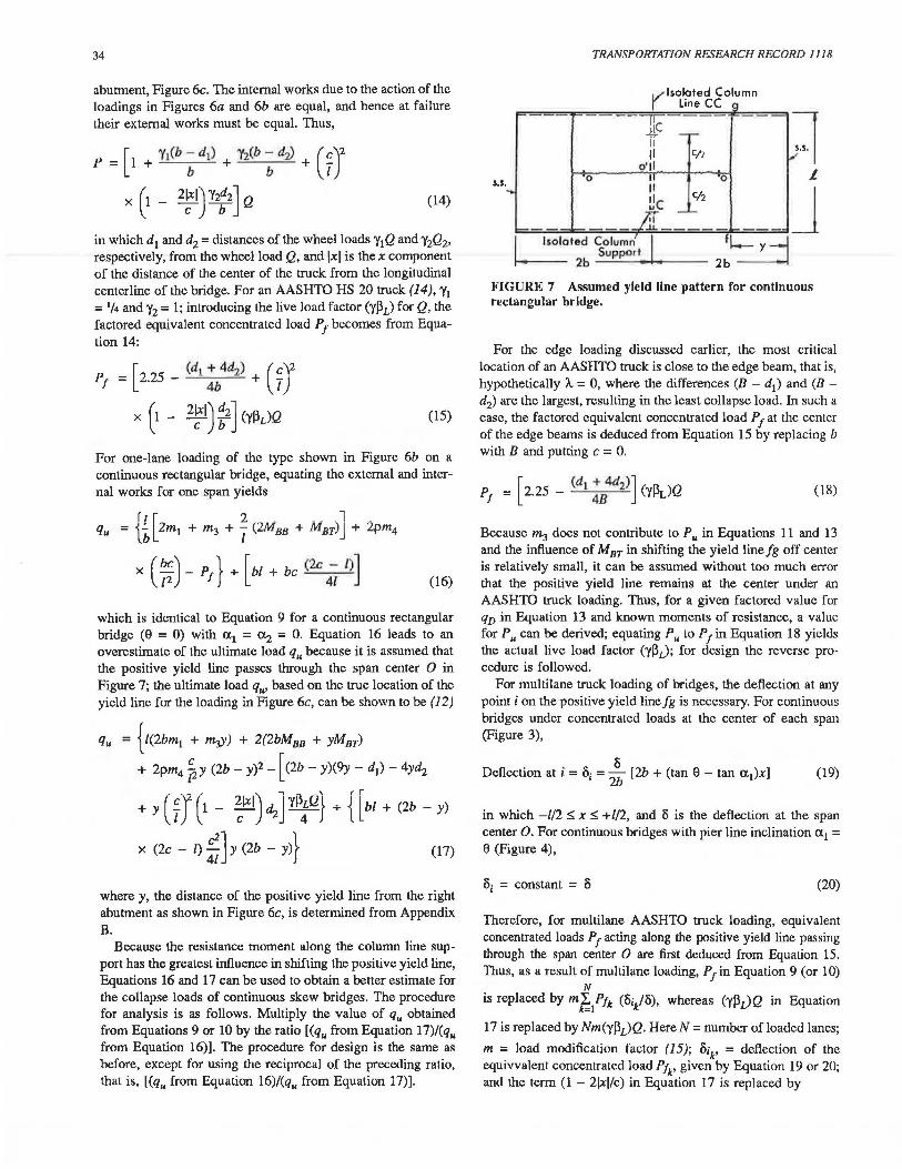
Collapse Load of a Bridge with Column Line Inclination cx1 = 0

For such a bridge the failure pattern is shown in Figure 4, with cx1 = 0 and <Xz = 0/2. Equating the external and internal virtual works yields the following expression for the ultimate uni­formly distributed load,

qu = { R11m1 + R12m3 + R13(2MBB + MBT)

+ (7)2 R14m4 - Pf} + {bl + (f )2 R19 } (10)

in which R11-R19 are defined in Appendix B. Equation 10 can be used for the following bridge geometries:

1. Two-span, continuous, skew bridge with continuous pier line support. Put c = 0, m4 = pm4 = 0.

2. Single-span bridge with parallel abutments. Put m3 = 0, M BT = 0, <Xz = 0/2, c = 0, m4 = pm4 = 0.

Kennedy

FIGURE 4 Assumed yield line pattern for continuous-skew bridge with o.1 = 0.

FIGURE 5 Assumed yield line pattern for continuous-skew bridge subjected to concentrated load near edge beam.

Concentrated Load Near an Edge Beam

It has been shown (12) that for such a loading the failure pattern can be assumed as shown in Figure 5. In this figure the concentrated load P is applied at a known distance 21..B from the center of the edge beam along the skew centerline JR, which makes an angle o.z with the x axis; 28 is the Jong span of an edge beam; Jg is a positive yield line, whereas gg' and gg" are negative yield lines. It is assumed that at failure the collapse load Pu and the uniformly distributed load q cause point f to deflect a distance o. By equating the external and internal virtual works, it can be shown that the collapse load is

Pu = { (4 cos o.2) [ m1 + 1nz + (Um1 + Tj!nz) tan2 0.2 - r q J

x y2 + (2MBB + MBT) y + r11n2 } + (y - A.) (11) B cos CXz

in which mz (Tltn.z) = ultimate negative moment of resistance in the slab per unit width (length) about the x (y) axis in the region of the edge beam; mz (Tltn.z) are not necessarily equal to ~ (~~) (see Figure 3); and 2yB is the unknown length of the yield line Jg. The nondimensional quantity y is given in Appen­dix B.

From the bridge geometries,

33

I B = b + 4 (tan 0 - tan o.1), and

(12)

When the concentrated load P is close to the center of the edge beam, a conservative value for the collapse load can be deduced by putting A.= 0 in Equation 11,

x tan2 o.z - ~ q J }1/2

(13)

The expressions for B and tan o.z (Equations 12) simplify according to the following bridge geometries:

1. Two-span, continuous, skew bridge with pier line perpen­dicular to the direction of traffic (i.e., cx1 = 0): B = b + (l/4) tan 0, tan o.z = 1/z tan 0.

2. Two-span, continuous, skew bridge with pier line parallel to the abutments (i.e., cx1 = 0): B = b, CXz = 0.

3. Two-span, continuous, rectangular bridge with pier line inclined an angle a 1 to the x axis: B = b + (//4) tan cx1,

tan 1/2o.z = tan cx1. 4. Two-span, continuous, rectangular bridge with cx1 = 0:

B = b, CXz = 0. 5. Simple-span, skew bridge with nonparallel abutments:

M8T = O; B and CXz are given by Equations 12. 6. Simple-span, skew bridge with parallel abutments: M BT=

O; B = b, CXz = 0.

Treatment of Truck Loads

The desired Equations 9-13 can be used to deal with AASIITO truck live loads, for example, the AASHfO HS 20 truck (14). Figure 6 shows a longitudinal section of a two-span, contin­uous, rectangular bridge loaded by a concentrated load P at the center 0 of one span through which a yield line passes, Figure 6a; an AASIITO HS 20 truck with the heaviest axle acting at O, Figure 6b; and an AASHTO HS 20 truck causing a yield line to form under the heaviest axle at a distance y from the right

'20 ~- d2 °1 a1 1rio ,q (c) ' I I I I I I I I I I I I I I iJ I I I I I I

(a) I t J I f t l I I I I I I I I l f 4 I 4 I l

0

b b

FIGURE 6 Longitudinal section of a continuous rectangular bridge under three loadings (a), (b), and (c).

34

abutment, Figure 6c. The internal works due to the action of the loadings in Figures 6a and 6b are equal, and hence at failure their external works must be equal. Thus,

(14)

in which d1 and d2 = distances of the wheel loads y1Q and y2Q2,

respectively, from the wheel load Q, and lxl is the x component of the distance of the center of the truck from the longitudinal centerline of the bridge. For an AASHTO HS 20 truck ( 14 ), y1 = 1/4 and y2 = 1; introducing the live load factor (YJ3L) for Q, the factored equivalent concentrated load P1 becomes from Equa­tion 14:

_ [ (d + 4d:z_) (c)2 P1 - 2.25 - 4b + T

x (1 - 2~1) :2 J (YJ3L)Q (15)

For one-lane loading of the type shown in Figure 6b on a continuous rectangular bridge, equating the external and inter­nal works for one span yields

qu = H[2m1 + m3 + T (2Mnn + MnT)] + 2pm4

x ( ~~) - P1 } + [bl + be (2c 4~ l) J (16)

which is identical to Equation 9 for a continuous rectangular bridge (0 = 0) with a 1 = az = 0. Equation 16 leads to an overestimate of the ultimate load qu because it is assumed that the positive yield line passes through the span center 0 in Figure 7; the ultimate load qu, based on the true location of the yield line for the loading in Figure 6c, can be shown to be (12)

qu = {t(2bm1 + my>) + 2(2bMBB + yMBT)

+ 2pm4 ~ y (2b - y)2 - [ (2b - y)(9y - d1) - 4yd2

+ y (f J (1 - ~!xi) dz J yJ3~Q} + { [bt + (2b - y)

x (2c - l) ~] y (2b - y)} (17)

where y, the distance of the positive yield line from the right abutment as shown in Figure 6c, is determined from Appendix B.

Because the resistance moment along the column line sup­port has the greatest influence in shifting the positive yield line, Equations 16 and 17 can be used to obtain a better estimate for the collapse loads of continuous skew bridges. The procedure for analysis is as follows. Multiply the value of qu obtained from Equations 9 or 10 by the ratio [(qu from Equation 17)/(qu from Equation 16)]. The procedure for design is the same as before, except for using the reciprocal of the preceding ratio, that is, [(qu from Equation 16)/(qu from Equation 17)].

TRANSPORTATION RESEARCH RECORD 1118

V Isolated Column J L' CC

s.s

me g

Tc ~

~ -~

II 11 C/l ...

o'll 0 " 0

· .... II c/2 ~c

hI -~

~

:1 I.

J I

ated Column I fl ,, y j Support

2b ------- 2b

FIGURE 7 Assumed yield line pattern for continuous rectangular bridge.

For the edge loading discussed earlier, the most critical location of an AASHTO truck is close to the edge beam, that is, hypothetically A. = 0, where the differences (B - d1) and (B -dz) are the largest, resulting in the least collapse load. In such a case, the factored equivalent concentrated load P1 at the center of the edge beams is deduced from Equation 15 by replacing b with B and putting c = 0.

[ (d1 + 4tfi)J Pl = 2.25 -

48 (yl\)Q (18)

Because m3 does not contribute to Pu in Equations 11 and 13 and the influence of M BT in shifting the yield line fg off center is relatively small, it can be assumed without too much error that the positive yield line remains at the center under an AASHTO truck loading. Thus, for a given factored value for qD in Equation 13 and known moments of resistance, a value for Pu can be derived; equating Pu to P1 in Equation 18 yields the actual live load factor (yJ3J; for design the reverse pro­cedure is followed.

For multilane truck loading of bridges, the deflection at any point i on the positive yield line fg is necessary. For continuous bridges under concentrated loads at the center of each span (Figure 3),

Deflection at i = O; = ! [2b + (tan 0 - tan a 1)x] (19)

in which -//2 :S x :S +//2, and o is the deflection at the span center 0. For continuous bridges with pier line inclination cx1 = 0 (Figure 4),

O; = constant = o (20)

Therefore, for multilane AASHTO truck loading, equivalent concentrated loads P1 acting along the positive yield line passing through the span center 0 are first deduced from Equation 15. Thus, as a result of multilane loading, P1 in Equation 9 (or 10)

N is replaced by m'ft,ttk (0;/15), whereas (yJ3JQ in Equation

17 is replaced by Nm(yJ3L)Q. Here N =number of loaded lanes;

m = load modification factor (15); Oik' = deflection of the equivvalent concentrated load Ptk' given by Equation 19 or 20; and the term (1 - 21xl/c) in Equation 17 is replaced by

KenMdy

1 [ ~ (1 - 271)~ N k=t IJ

The term lxkl is the x component of the distance between the longitudinal centerline of an AASHTO truck loading and the longitudinal centerline of the bridge.

For loads applied near an edge beam, it is reasonable to expect that only one AASHTO truck loading can be accommo­dated in that region; therefore, for this case multilane loading is not applicable.

As a worked design example, it is required to estimate the longitudinal positive moment m1, at midspan for a two-span, continuous, skew, waffle slab bridge having a continuous pier line support (i.e., c = 0). The plan of the bridge is similar to the plan of Category I bridges shown in _Figure 2a, with the following data: a.1 = 45°; 0 = 45°; length of each span 2b = 90 ft (27.43 m); three 12-ft traffic lanes with a total bridge width l = 42 ft 3 in. (12.88 m). Consider qD = 0.34 kip/ft2 (16.27 kPa); AASHTO HS 20 truck loading with d1 = d2 = 14 ft (4.27 m). Assume the following moment ratios: u = 0.6; TJ = 1.0; ~ = 0.6; p = 0.6; m1/m2 = 1.5; m1/~ = 0.8; m1/m4 = 2.0. Take M88 = 760 kip-ft (1.03 MN-m) and MBT = 850 kip-ft (1.15 MN-m). The factored dead load qu = 1.3 (0.34) = 0.44 kip/ft2 (21.75 kPa); the live load factor (yPJ = 1.3[ 1.67(1 +impact factor)] = 2.17[1+50/(125 + 90)] = 2.67. From Equation 15 (with c = 0) and Q = 32 kip (142.2 kN), P1 = [2.25 - 70/180](2.67)(32) = 159 kip (707.6 kN). For a three-lane loading, P1 is replaced by

3 m I, Pfk (o;/6)

k=l

with m = 0.90, Because cx1 = 0, Equation 20 yields

011 :: 512 = Oi3 = o; and, because c = 0,

1herefore, the term

3 mt:/tk (oi/o) = 0.9(P1o + P1o + Pt°)fo

= 2.10P1 = 429.3 kip (1,910 kN).

Using Equation 10 (because cx1 = 0), with qD = qu = 0.44 kip/ft2

(21.75 kPa), P1 = 429.3 kip (1,910 kN) and the other relevant data, yield m1 = 310 kip-in.fin. (1.38 MN-m/m). For a more refined solution, qD = 0.44 kip/ft3 is first augmented by the ratio [(qu from Equation 16)/(qu from Equation 17)] = 1.01 with y = 35.9 ft (10.95 in.). Using qu = (0.44)(1.01) in Equation 10 leads to m1 = 313 kip-in.fin. (1.39 MN-m/m). Applying a perfor­mance factor of cl>= 0.9, then m1 becomes 348 kip-in.fin. (1.55 kN-m/m). Hence, the other moments can now be estimated from m1 and the assumed ratios. Preliminary calculations show that the following bridge geometry is adequate to provide the specified moments of resistance: 8 in. (200 mm) deck; 33 in. deep x 8 in. wide ribs; 6-ft spacing for longitudinal ribs; 8-ft 6-in. spacing for transverse ribs; ratio of pres tressing steel = 0.5 percent; additional mesh steel reinforcing is required for local bending in the deck.

As illustrated in the preceding example, it is necessary in design to assume realistic values for the moment ratios u, TJ, p,

35

m1/mi, m1/~, and m1/m4, based on previous experience, and on available results from an elastic analysis. It is recommended that in the longitudinal direction. ratios of negative to positive ultimate moments of resistance per unit width between 1 and 1.3 should be used; ratios of the ultimate moments of resistance per unit width in the transverse and longitudinal directions may vary from 0.5 to 1.0 depending on the aspect ratio of the bridge, edge support conditions, and the location on the bridge. In order to minimize cracks and crack widths, it is necessary also to vary the distribution of the required steel along the yield lines, following the elastic bending moments as closely as possible, for example, more negative steel near the column strips than in the middle strips. Furthermore the ultimate load method of design does not recognize the presence of large torsional moments and hence steep strain gradients at the cor­ners and support regions of such bridges; therefore, these regions require special attention in design. Other construction details for this type of bridge structure include layouts of the prestressing steels and anchorage, provisions for the obtuse and acute corners, type of supports, and reinforcing the deck. These issues will be addressed in a forthcoming paper.

In the analysis of a bridge that has been designed elastically, the equations derived here can be used to estimate the values of the collapse load qu or Pu• and hence the corresponding load factors (YPv) and (YPL) on the design loading. Although these equations are for two-span bridges, they can also be used to give conservative results for bridges with three or more spans.

ORTHOGONAL VERSUS NONORTHOGONAL RIB CONSTRUCTION

Although it is obvious that an orthogonal rib design (i.e., ribs orthogonal to the flow of traffic) is the correct configuration for rectangular bridges, it may not be so for skew bridges. To investigate this problem. tests were carried out on three bridge models (16) each having the same skew angle, self-weight, span, and width; the three structures were of the orthogonal­nonorthogonal-rib waffle slab constructions and solid-slab con­struction. The test results revealed that the orthogonal rib waffle slab construction for skew bridges can be expected to have the following advantages over the other two con­structions: (a) a better load distribution characteristic; (b) a superior stiffness and ultimate load-carrying capacity; and (c) less severe stress concentration at the critical obtuse corners.

DYNAMICS OF WAFFLE SLAB BRIDGES

The dynamic response of waffle slab bridges was studied re­cently (17). The analytical study was verified and substantiated by experimental results from tests on prestressed and rein­forced waffle slab bridge models. The study showed that by increasing the stiffness by means of prestressing, the natural frequencies of the bridge are significantly enhanced; this phe­nomenon helps in avoiding resonance under low-frequency excited sources of vibration. Furthermore, to demonstrate the advantage of using waffle slab versus solid-slab construction the dynamic responses of the two types of construction having the same self-weight and planforrn geometry were compared. The natural frequency of the waffle slab bridge was 65 percent

36

greater than the one for the solid-slab bridge; this result was expected because the longitudinal and transverse rigidities of the waffle slab bridge were much greater than those of the solid-slab bridge. Furthermore, the first natural frequency of a waffle slab bridge appears to be greater than any vehicle frequencies, which are in the range 2-5 Hz, thus leading to a much lower dynamic load allowance used in design.

OTHER OBSERVATIONS

The presence of transverse ribs in the waffle slab bridge has additional advantages regarding the serviceability limit states. First, the transverse ribs make it possible to locate the pre­stressing steel at varying levels of eccentricity, leading to better control, possible elimination of longitudinal cracking of the deck, and reduced final deflections. Second, the transverse ribs are also important for providing crack control around the ob­tuse comers of skewed concrete bridge structures where com­plicated stress fields exist. Third, the transverse ribs help in reducing local deformation due to heavy wheel loads on the bridge deck for better live-load distribution. Furthermore, the shallower cross-sectional depth in waffle slab construction in comparison to the one-way ribbed-slab (T-beam) construction would result in smaller cost for bridge approaches.

Although construction details of this type of bridge will be addressed elsewhere, some brief comments on practical design are in order here. While prestressing in two directions may eliminate all tensile stresses in a waffle slab rectangular bridge, the same may not be possible in a waffle slab skew bridge. In the latter bridge, the direction of the top-surface principal stresses deviate considerably from those of the bottom-surface principal stresses as well as from the direction of prestress; this is especially so around the obtuse comers. To eliminate all tensile stresses in such cases requires excessively high levels of prestress and hence a heavier cross section, which may not be economical. It is more practical instead to provide untensioned reinforcement to resist local stresses when they occur. This refinement may be calculated in a similar way as in reinforced­concrete construction; the axial forces induced by the prestress in the steel reinforcement are ignored. It is suggested that, for crack control, the minimum percentage of untensioned steel in the transverse direction should be about 0.15 percent (1 ). It is also important to remember to reduce the maximum compres­sive stress around the acute corners of waffle slab skew bridges by curtailing alternate prestressing cables in those regions.

It is usual practice to make the waffle solid over column supports; furthermore, shear requirements dictate the use of tapered pans near the exterior supports. In cases where moment connections are not necessary, low-friction pads such as Teflon or Tetron are suggested for bearings. Such bearing details normally provided in bridges to permit thermal changes are well suited to accommodate elastic shortening and rotation due to posttensioning.

Finally, one can expect prestressed waffle slab bridges to be much stiffer and stronger than similar bridges in reinforced concrete construction and with a smaller amount of secondary stress produced by sustained loads. In general, prestressed concrete construction also becomes more attractive in situa­tions where construction depth is at a premium.

TRANSPORTATION RESEARCH RECORD 1118

CONCLUSION

This study has shown that waffle slab bridges have the potential of being an economical alternative to other types of bridges. This economic advantage becomes greater with increase in width-to-span ratio or in skew angle of the bridge. The waffle slab construction, besides affording excellent access for inspec­tion and maintenance of salt damage to prestressing steel, also reduces the dead load moment and deflection; these effects minimize the amount of secondary stresses produced by sus­tained loads. Furthermore, such bridges have a much superior dynamic response. The results presented herein provide the designer with aids for design and analysis of simple- and continuous-span waffle slab bridges.

REFERENCES

1. P. Csagoly and M. Holowka. Cracking of Voided Post-Tensioned Concrete Bridge Decks. Research Report 193. Ministry of Trans­portation and Communications, Downsview, Ontario, Canada, 1975.

2. T. Y. Lin, F. Kulka, and Y. C. Yang. Post-Tensioned Waffle and Multispan Cantilever System with Y-Piers Composing the Hegen­berger Overpass. Concrete Bridge Design, SP23-27. American Concrete Institute, Detroit, Mich., 1969. pp. 495-506.

3. R. H. Wood. The Reinforcement of Slabs in Accordance with a Predetermined Field of Moments. Concrete, Vol. 2, No. 2, 1968, pp. 69-76.

4. J. B. Kennedy and B. Bakht. Feasibility of Waffle Slabs for Bridges. Canadian Journal. of Civil Engineering, Vol. 10, No. 4, 1983, pp. 627-638.

5. Suite of Bridge Design and Analysis Program HECBIB/13 STRAND (Version 1) User: Parts 1 and 2. Department of the Environment, London, England, 1974.

6. J. B. Kennedy and S. K. Bali. Rigidities of Concrete Waffle Slab Structures. Canadian Journal. of Civil Engineering, Vol. 6, No. 1, 1979, pp. 65-74.

7. J.B. Kennedy and I. S. El-Sebakhy. Waffle Slab Concrete Bridges: Ultimate Behaviour. Journal of the Structural Division, ASCE, Vol. 108, No. ST6, 1982, pp. 1285-1301.

8. K. J. Bathe, E. L. Wilson, and F. E. Paterson. A Structural Anal­ysis Program for Static and Dynamic Response of Linear System (SAP IV). Report EERC 72-11. Earthquake Engineering Research Center, University of California at Berkeley, April 1974.

9. H. T. Huber. Die Theorie der Kreuzweise Bewehrtren Eisen­betonplatten Nebst Anwendungen auf Mehrere Bautechnisch Wichtige Aufgaben uber Rechteckige Platten. Der Bauingenieur, Vol. 4, 1923, pp. 354-360.

10. S. 'Iimoshenko and J. N. Goodier. Theory of Elasticity. McGraw­Hill Book Co., New York, 1970, p. 312.

11. M. A. Saeed and J. B. Kennedy. Time-Dependent Deformation in Prestressed Concrete. Symposium on the Design of Concrete Structures for Creep, Shrinkage, and Temperature Changes, Inter­national Association for Bridge and Structural Engineering, Madrid, Spain, 1970, pp. 217-227.

12. J. B. Kennedy and I. S. El-Sebakhy. Ultimate Loads of Orthotropic Bridges Continuous Over Isolated Interior Supports. Canadian Journal of Civil Engineering, Vol. 12, No. 3, 1985, pp. 547-558.

13. I. S. El-Sebakhy and J. B. Kennedy. Progressive Failure Analysis of Orthotropic Bridges. Journal of Structures and Computers, Vol. 24, No. 3, 1986, pp. 401-411.

14. K. W. Johansen. Yield-Line Theory. Translation, Cement and Con­crete Association, London, England, 1962.

15. Standard Specifications for Highway Bridges, 12th ed., AASHTO, Washington, D.C., 1977.

Kennedy

16. J. B. Kennedy. Orientation of Ribs in Waffle-Slab Skew Bridges. Journal of Structural Engineering. Vol. 109, No. 3, March 1983, pp. 811-816.

17. N. F. Grace. Free Vibration of Prestressed Continuous Composite Bridges and Skew Orthotropic Plates. Ph.D. dissertation, Univer­sity of Windsor, Ontario, Canada, 1986.

APPENDIX A

The following define the tenns introduced in the section Elastic Analysis:

e = x [b./lx;(h + dj2) + (n - l)A8

X (h + dx - d') + a.}12/2(1 - µ2)] + [b,..dx + (n - l)A8 + a.}1/(1 - µ2)]

ey = [b1dy01 + d.J2) + (n - l)A/ x (11 + dY - d") + a/'2/2(1 - µ2)] + [bi>' + (n - l)As + a/1/(l - µ2)]

Ix' = b,..dx[(h + d)2) - ex]2

+ (n - l)A8 [(h + dx - d') - ex]2

+ b,_.dx3/12 ly' = biyl(h + d/7:) - eyl2

+ (n - l)A/ [(h + d1

- d") - ey]2

+ bi/112

where

n bx (by) dx (dy)

d' (d'')

A8 (A/)

Dx' (Dy')

lex = ax<kdx)3(3

Icy = a/kdy)3(3

= = =

=

=

=

modular ratio; width of longitudinal (transverse) rib; depth of the longitudinal (transverse) rib; concrete cover to the center of the longitudinal (transverse) prestressing steels; area of prestressing steel in the longitudinal (transverse) rib; and flexural rigidity of the deck with respect to the neutral plane of the gross cross section associated with bending in the x (y) direction.

lsx = nA8 [(h + dx - d') - kdx]2

lsy = nA/[(h + dy - d'') - kdy]2

The location of the neutral axis kdx (or kdy) is determined by equating the tension force to the compression force on the section. Thus, by assuming that the neutral axis lies in the deck, kdx is given by

and kdy by

nA/[(h + dy - d'') - kdyl - Oy(kdy)2/2(1 - µ2) = 0

37

APPENDIX B

The following terms appear in the section Ultimate Load Analysis.

R1 = ~(in which 2b is the length of each span)

'U(Lan 0 + tan CJ.1)2

R - 2 + ------""--2 - 2

[Note: When R7 ~ 0, put R7 ln R8 = O.]

R5 = -b sin~ - (~)(cos~+ tan a.1 sin~

b sin~ R6 = 1 + R

5

R1 = b sin~ - (~)(cos~+ tan a.1 sin~

R 1 _ b sin~

8 = R1

(4802 + /2(tan 0 - Lan a,i)2]/ R9 = 48b

bl 12

Rio = -2

- Sb . 2 (R5 ln R6 + R1 ln R8) COS CX-;? Siii CX-;?

Ru = 2(tan ~J1 (cos2 ~ + u sin2 ~)

x [1n(2b cos0 + Itani)- ln( 2b cos0 - /tan~)]

[Note: When 0 = 0, put Ru = ~I ·]

R12 = (tan ;)-l (cos2 0 + ~ sin2 0)

x {1n [ 2b cos2 0 + (b sin2 0 + b)tan i]

- ln [ 2b cos2 0 + (b sin2 0 - l) tan ~] }

[Note: When 0 = 0, put R12 = t ·] R

_ Sb cos2 0 13 - 0

4b2 cos2 0 - /2 tan2 -2

38

[Note: When R17 :s; 0, put R 11 In R18 = O.]

Ris = (-2b cos 0 sin~ - c cos~)+ 2 cos 0

R16 = [ 1 + (~)cos 0 tan ~r1

R11 = (2b cos 0 sin~ - c cos ~) + 2 cos 0

Ru = [ 2b 1 "] 1-c-cos0tan 2

The nondimensional quantity y in Equation 11 is derived from the stationary condition (JP/(Jy = 0, namely

y2 - (21..)y . c = 0

where

x tan2 <X.i - (B2/6)q]}

TRANSPORTATION RESEARCH RECORD 1118

The distance y of the positive yield line from the right abutment, shown in Figure 6c, is determined from the station­ary value of qu in Equation 17, that is, oq uloy = 0, resulting in the following equation for y:

in which

R20 = [c3 + (2b)c4 + c5]c9 - c4c8 R21 = 2[c2 - (2b)c5 - c6 + c7]c9 + (4b)c4c8 R22 = [3c1 - (2b)(c2 - 2bc5 - c6 + 4c7)]c9

+ [c2 + (2b)c3 - c6 + c7]cs R23 = [2c1 - (4b)c7][c8 - (2b)c9]

R24 = (-2b) [c1 - (2b)c7]c8

where

c1 = 2b(lm1 + 2MBB)

C2 = I~ + 2M BT + 8pm4cb2//2

c3 = -8pm4cb/12

c4 = 2pm4c//2

C5 = 2.25 ("f~JQ

C7 = -dl ("f~JQ/4

be (2c - l) c8 = bl +

21 ; and

(I - 2c) c C9 = 41

Publication of this paper sponsored by Committee on Concrete Bridges.