presentation SEN 2012 - nuclear.ufrj.br presentation SEN... · 0 60 120 180 240 300 360 0 2 4 6 8...
51
Fluidodinâmica Computacional Paulo A. B. de Sampaio – IEN/CNEN Alvaro L.G.A. Coutinho – PEC/COPPE/UFRJ Milton Alves Gonçalves Jr. - PEC/COPPE/UFRJ Marcos Filardy Curi – IEN/CNEN II Semana de Engenharia Nuclear I International Symposium of Nuclear Engineering 13-17 de Agosto de 2012, UFRJ, Rio de Janeiro - RJ
Transcript of presentation SEN 2012 - nuclear.ufrj.br presentation SEN... · 0 60 120 180 240 300 360 0 2 4 6 8...
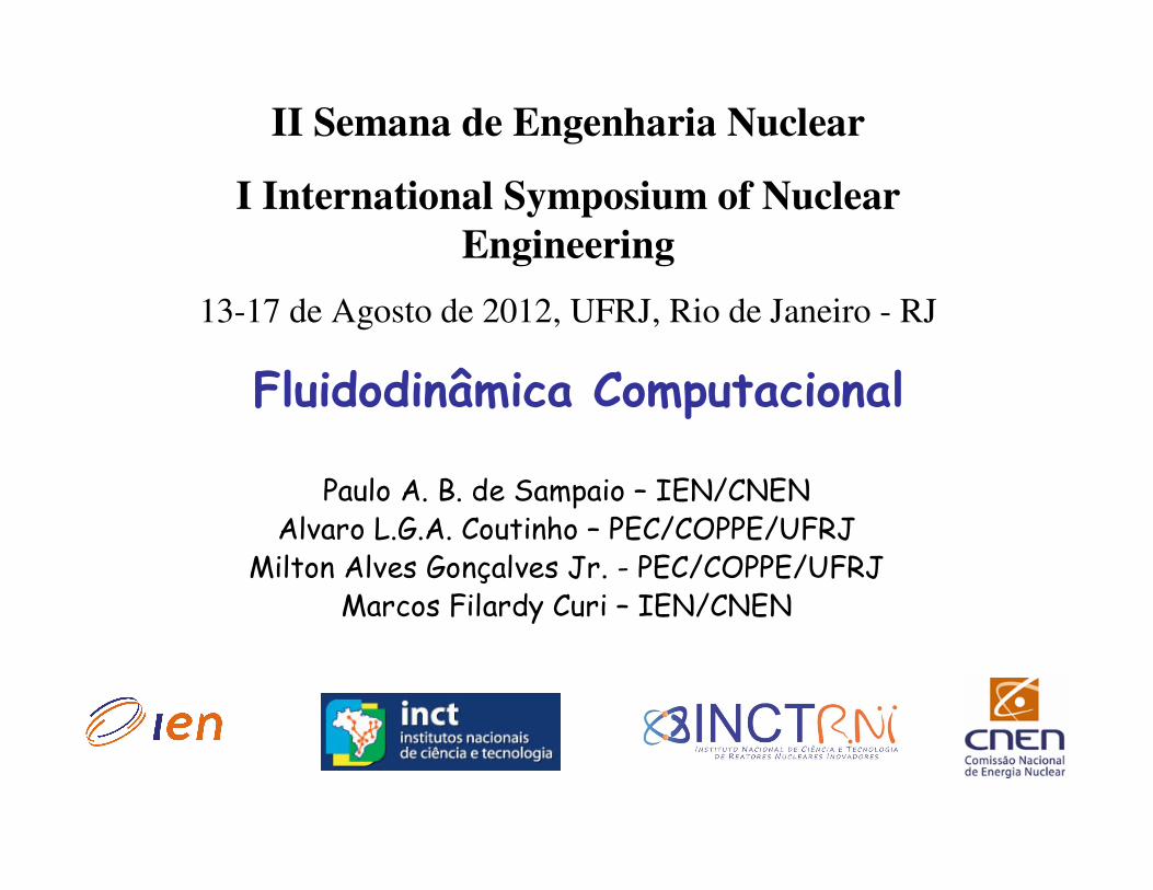
Fluidodinâmica Computacional
Paulo A. B. de Sampaio – IEN/CNENAlvaro L.G.A. Coutinho – PEC/COPPE/UFRJ
Milton Alves Gonçalves Jr. - PEC/COPPE/UFRJMarcos Filardy Curi – IEN/CNEN
II Semana de Engenharia Nuclear
I International Symposium of Nuclear Engineering
13-17 de Agosto de 2012, UFRJ, Rio de Janeiro - RJ

Topics
Introduction
Incompressible viscous flow model
Deriving stable finite element formulations
Numerical examples
Some new developments
Concluding remarks

Introduction
The drawbacks of the Galerkin mixed formulation for incompressible viscous flows:
1. Occurence of wiggles (spatial oscillations of the solution) in convection-dominated flow problems.
2. Restrictions on the choice of interpolating spaces for velocity and pressure.

Introduction
Stabilised finite element methods can be used to overcome deficiencies of the Galerkin method when applied to flow problems.
Examples: 1. Controlling wiggles in convection-dominated flow problems; 2. Circumventing the Babuska-Brezzi condition for incompressible flows modelled by N-S equations in primitive variables (u, p).

Introduction
Stabilised finite element methods can be often interpreted as Petrov-Galerkin weighted residual approximations, where the Galerkin weighting function is modified with the addition of a perturbation.
The terms resulting from the interaction of the perturbation with the residual generate the desired stabilization effect, without compromising the consistency of the approximation.

Introduction
In this work we present a framework for deriving stable finite element formulations for coupled flow problems.
The “stabilising terms” emerge naturally in the derivation, rather than being introduced a priori in the variational formulation of the problem.

Flow and Heat Transfer Model
Incompressible N-S equations with buoyancy force and a convection-diffusion energy equation.
( ) 0TTgβρx
p
x
τ
x
uu
t
uρ 0a
ab
ab
b
ab
a =−+∂
∂+
∂
∂−
∂
∂+
∂
∂
0=∂
∂
a
a
x
u
0=∂
∂+
∂
∂+
∂
∂
b
b
b
bx
q
x
Tu
t
Tcρ
( )abbaab xuxu ∂∂+∂∂= µτ
bb xTq ∂∂−= κ(with the usual i.c and b.c.)

Flow and Heat Transfer Model
In some applications we may also consider the transport and radioactive decay of radionuclides.
0=+∂
∂+
∂
∂+
∂
∂φλ
ξφφ
b
b
b
bxx
ut
0=−∂
∂+
∂
∂+
∂
∂φλ
ηϕϕ
b
b
b
bxx
ut
bb x∂∂−= φψξ bb x∂∂−= ϕςη
with diffusive fluxes given by Fick’s Law


Numerical Examples
Cylinder in cross flow (forced convection)
Mesh transientfor Re=100

Numerical Examples
Cylinder in cross flow (forced convection)
Force coefficients for Re=100, 125 and 150
-0,6-0,4-0,2
00,20,40,60,8
11,21,41,6
0 20 40 60 80 100 120 140 160 180 200
Time
Fo
rce
Co
effic
ien
ts
CD
CL
-0,6-0,4-0,2
00,20,40,60,8
1
1,21,41,6
0 20 40 60 80 100 120 140 160 180 200
Time
Fo
rce
Co
effi
cien
ts
CD
CL
-0,6-0,4
-0,20
0,20,40,60,8
11,2
1,41,6
0 20 40 60 80 100 120 140 160 180 200
Time
Fo
rce
Co
effi
cien
ts
CD
CL
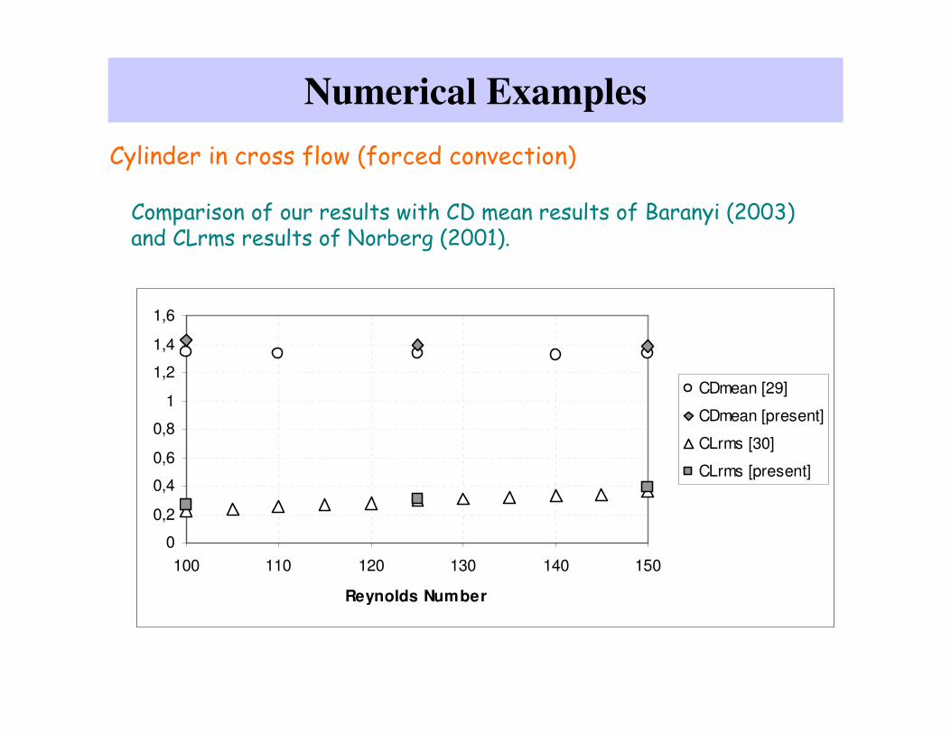
Numerical Examples
Cylinder in cross flow (forced convection)
Comparison of our results with CD mean results of Baranyi (2003)and CLrms results of Norberg (2001).
0
0,2
0,4
0,6
0,8
1
1,2
1,4
1,6
100 110 120 130 140 150
Reynolds Number
CDmean [29]
CDmean [present]
CLrms [30]
CLrms [present]

Numerical Examples
Cylinder in cross flow (forced convection)
Comparison of our results with Strouhal number results of Williamson (1988)
0,15
0,16
0,17
0,18
0,19
0,2
100 110 120 130 140 150
Reynolds Number
Strouhal [31]
Strouhal [present]
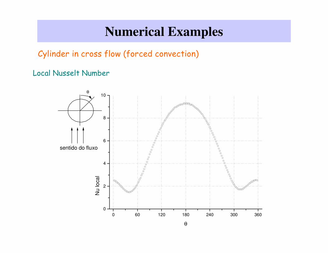
Numerical Examples
Cylinder in cross flow (forced convection)
Local Nusselt Number
0 60 120 180 240 300 3600
2
4
6
8
10N
u lo
cal
θ
θ
sentido do fluxo

Numerical Examples
Cylinder in cross flow (forced convection)
Mean Nusselt Number
100 110 120 130 140 1505,0
5,5
6,0
6,5 Nu - obtido Nu - Lange et al. [36] Nu - Bernstein et al. [35]
Nu
Número de Reynolds

Numerical Examples
Free convection around a hot horizontal cylinder
Temperature field and adaptive mesh for Pr=0.71, Ra=100000

Numerical Examples
Free convection around a hot horizontal cylinder
Temperature field and adaptive mesh for Pr=0.71, Ra=100000
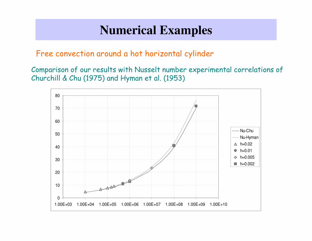
Numerical Examples
Free convection around a hot horizontal cylinder
Comparison of our results with Nusselt number experimental correlations of Churchill & Chu (1975) and Hyman et al. (1953)
0
10
20
30
40
50
60
70
80
1.00E+03 1.00E+04 1.00E+05 1.00E+06 1.00E+07 1.00E+08 1.00E+09 1.00E+10
Nu-Chu
Nu-Hyman
h=0.02
h=0.01
h=0.005
h=0.002
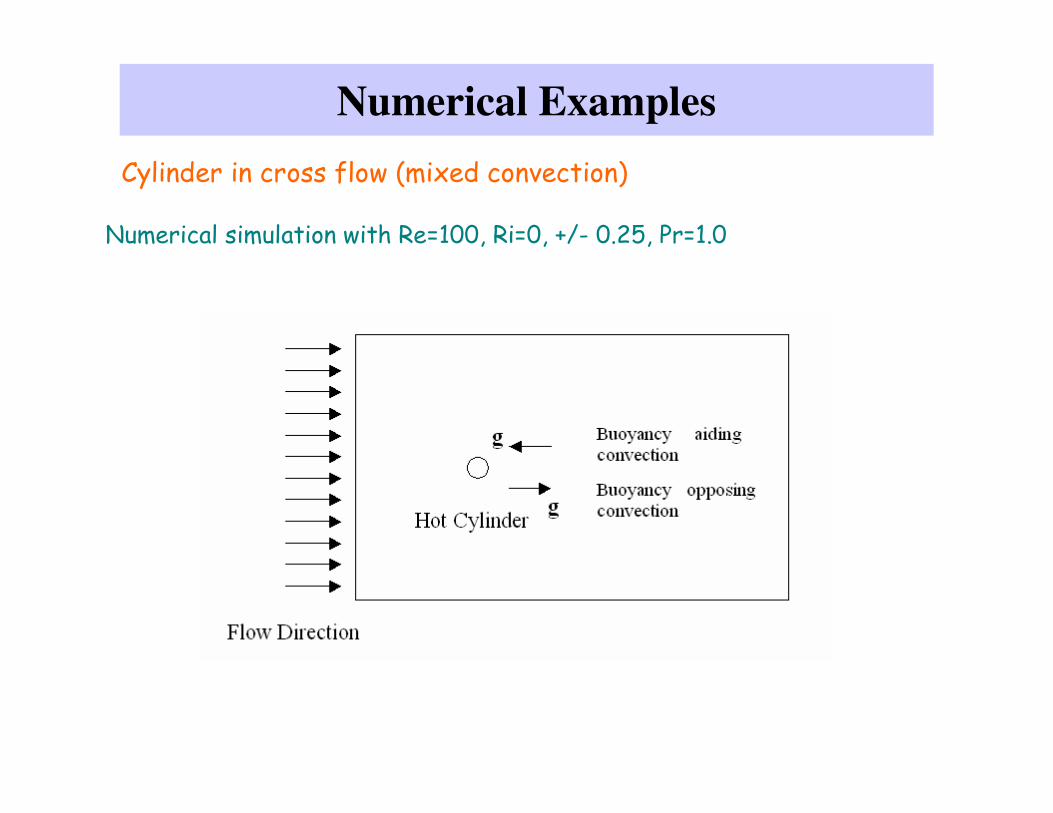
Numerical Examples
Cylinder in cross flow (mixed convection)
Numerical simulation with Re=100, Ri=0, +/- 0.25, Pr=1.0

Numerical Examples
Cylinder in cross flow (the effect of the Ri number):
Re=1000 ; Ri=0 (forced convection only)

Numerical Examples
Cylinder in cross flow (the effect of the Ri number):
Re=1000 ; Ri=1 (buoyancy aiding convection)
Numerical Examples
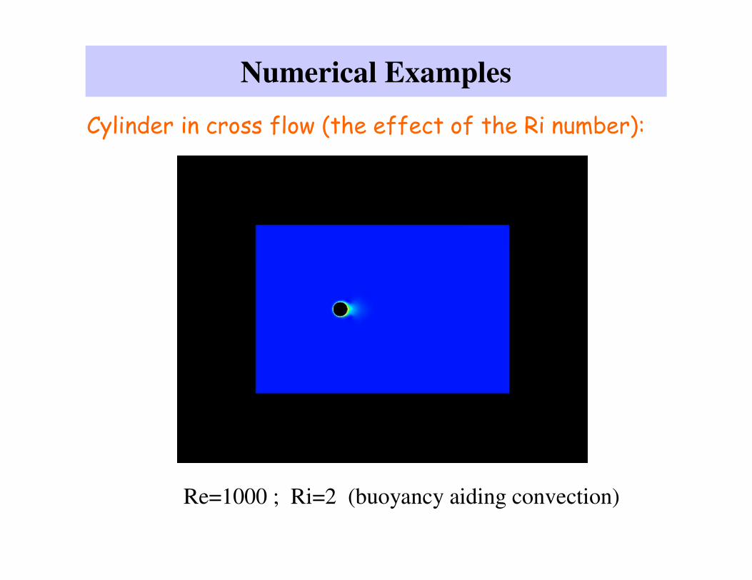
Cylinder in cross flow (the effect of the Ri number):
Re=1000 ; Ri=2 (buoyancy aiding convection)

Numerical Examples
Cylinder in cross flow (the effect of the Ri number):
Re=1000 ; Ri=1 (buoyancy opposing convection)
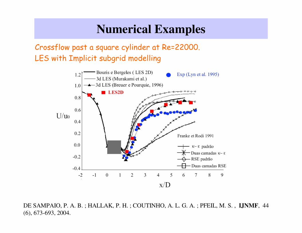
Numerical ExamplesCrossflow past a square cylinder at Re=22000.
LES with Implicit subgrid modelling
DE SAMPAIO, P. A. B. ; HALLAK, P. H. ; COUTINHO, A. L. G. A. ; PFEIL, M. S. , IJNMF, 44 (6), 673-693, 2004.
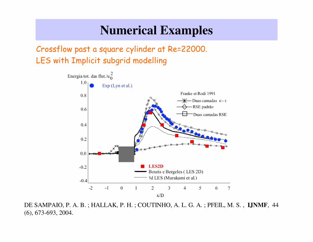
Numerical ExamplesCrossflow past a square cylinder at Re=22000.
LES with Implicit subgrid modelling
DE SAMPAIO, P. A. B. ; HALLAK, P. H. ; COUTINHO, A. L. G. A. ; PFEIL, M. S. , IJNMF, 44 (6), 673-693, 2004.

Numerical ExamplesRio-Niteroi Bridge (Reynolds 5.8E+6 to 1.0E+7).
ALE + LES with Implicit subgrid modelling
DE SAMPAIO, P. A. B. ; HALLAK, P. H. ; COUTINHO, A. L. G. A. ; PFEIL, M. S. , IJNMF, 44 (6), 673-693, 2004.

Some new developments
01
2
2
=
∂
∂
∂
∂+
∂
∂−
∂
∂+
∂
∂+
∂
∂+
∂
∂
r
ur
rrx
u
x
P
r
uv
x
uu
t
uµρ
01
22
2
=
−
∂
∂
∂
∂+
∂
∂−
∂
∂+
∂
∂+
∂
∂+
∂
∂
r
v
r
vr
rrx
v
r
P
r
vv
x
vu
t
vµρ
( ) 01
=∂
∂+
∂
∂rv
rrx
u
Momentum balance (axial)
Momentum balance (radial)
Mass balance
Axissymmetric Problems
Some new developments
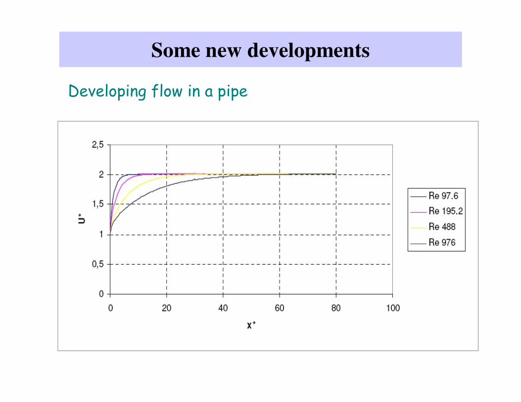
Developing flow in a pipe

Some new developments
Developing flow in a pipe

Some new developments
Developing flow in a pipe

Some new developments
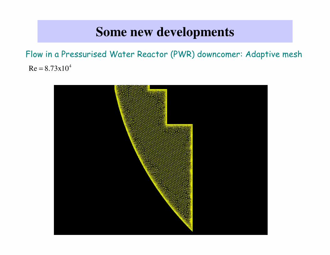
Flow in a Pressurised Water Reactor (PWR) downcomer

Some new developments
Flow in a Pressurised Water Reactor (PWR) downcomer: Velocity field410x73.8Re =
Some new developments
Flow in a Pressurised Water Reactor (PWR) downcomer: Adaptive mesh410x73.8Re =

Some new developments
Alternative time discretisation of convection:
So far we have used
b
n
an
bx
uu
∂
∂ + 2/1
which is formally )( tO ∆
But if this is replaced by
∂
∂+
∂
∂ ++
b
n
an
b
b
n
an
bx
uu
x
uu 1
1
2
1 we obtain )( 2tO ∆
In this case the equations for updating the velocity components become fully coupled.
Some new developments
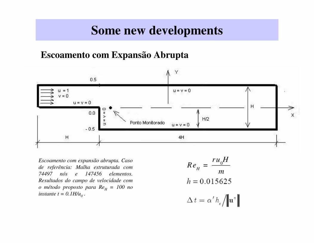
Escoamento com Expansão Abrupta
Escoamento com expansão abrupta. Caso
de referência: Malha estruturada com
74497 nós e 147456 elementos.
Resultados do campo de velocidade com
o método proposto para ReH = 100 no
instante t = 0.1H/u0 .
0H
u HRe
r
m=
Some new developments
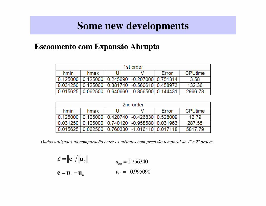
Dados utilizados na comparação entre os métodos com precisão temporal de 1ª e 2ª ordem.
bε = e u
r b= −e u u
0 0.756340bu =
0 0.995090bv = −
Escoamento com Expansão Abrupta

Some new developments
Escoamento com Expansão Abrupta
Erro relativo da velocidade e tempo de CPU para os métodos de 1ª e 2ª ordem. Exemplo de um transiente rápido em
diferentes níveis de refinamento.

Some new developments
Implementação 3D
Características Método original - EdgeCFD® Método presente
Discretização Espacial Temporal Temporal Espacial
Termos de estabilização SUPG / PSPG / LSIC (a priori) Surgem naturalmente
Modelo de turbulência LES – Smagorinsky / VMS LES - Implícito
Sistemas de equações
EDOs não lineares totalmente
acopladas u-p (4 graus de liberdade
por nó). Não simétricas.
Algébricas lineares
parcialmente acopladas
p u. Simétricas,
positivo-definidas.
Esquema de integração temporal Preditor / Multi-corretor Não possui
Solver não linear Newton Inexato Não possui
Solver linear GMRES PCG
Estrutura de dados Aresta por aresta Aresta por aresta
Implementação paralela MPI/OpenMP/Híbrida MPI/OpenMP/Híbrida

Some new developments
Cavidade – 3D
Escoamento induzido no interior de uma
cavidade 3D pelo movimento de uma tampa.
Malha não estruturada com 108104
elementos tetraédricos e 20589 nós.
Linhas de corrente no escoamento induzido
no interior de uma cavidade 3D pelo
movimento de uma tampa para ReL = 100.
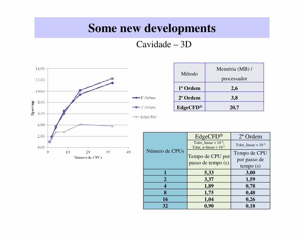
Some new developmentsCavidade – 3D
MétodoMemória (MB) /
processador
1ª Ordem 2,6
2ª Ordem 3,8
EdgeCFD® 20,7
Número de CPUs
EdgeCFD® 2ª OrdemToler_linear = 10-3;
Toler_n-linear = 10-3. Toler_linear = 10-3
Tempo de CPU por passo de tempo (s)
Tempo de CPU por passo de
tempo (s)1 5,33 3,002 3,37 1,594 1,89 0,788 1,75 0,4816 1,04 0,2632 0,90 0,18

ESTUDOS DE LIMITES TERMO-HIDRÁULICOS PARA PROJETO DE VARETAS COMBUSTÍVEL
DE REATORES NUCLEARES
Paulo Augusto Berquó de Sampaio
Maria de Lourdes Moreira
Isaque de Souza Rodrigues
João Carlos Aguiar Gaspar Junior
Renato Raoni
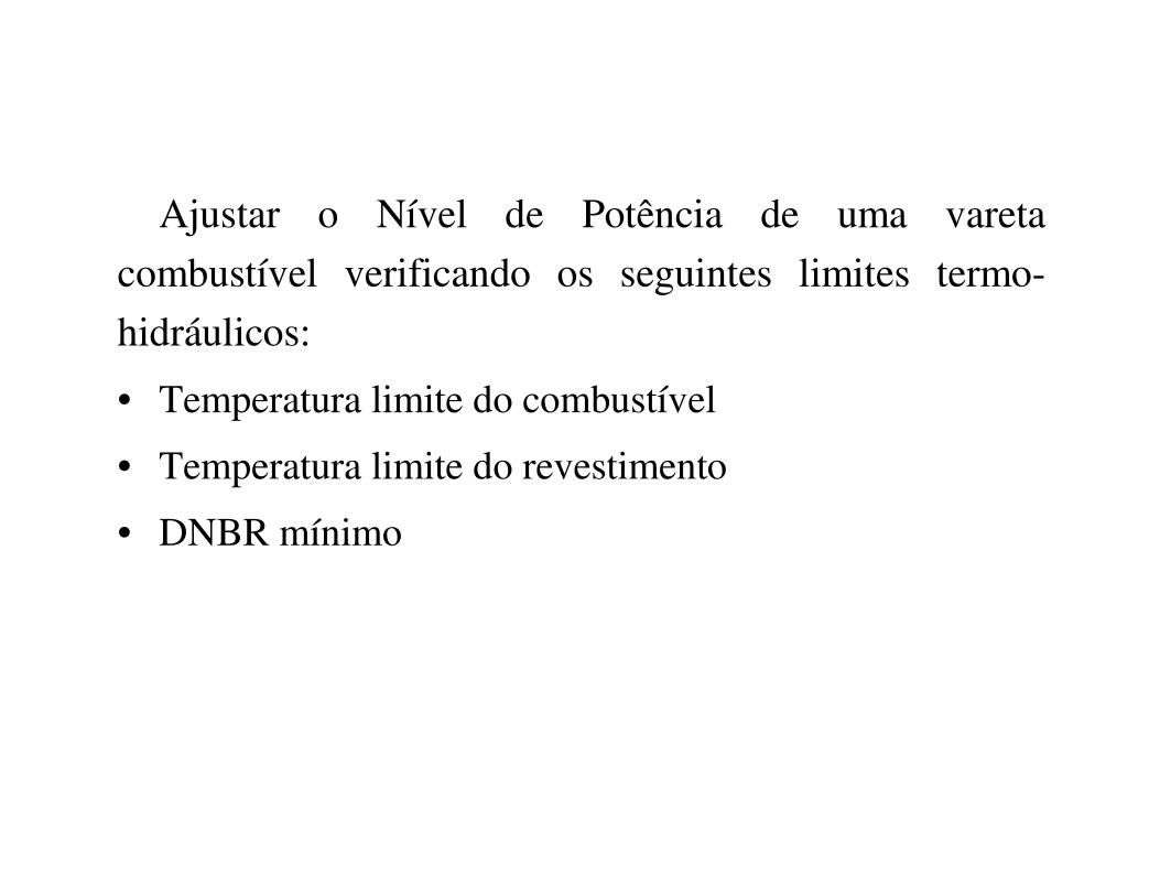
Ajustar o Nível de Potência de uma vareta
combustível verificando os seguintes limites termo-
hidráulicos:
• Temperatura limite do combustível
• Temperatura limite do revestimento
• DNBR mínimo

MODELAGEM FÍSICA- Discretização axial
-1830
-915
0
915
1830
q```
z
Distribuição da taxa volumétrica de geração de calor [ q’’’(z) ] ao longo da vareta combustível
( )
+=′′′ z
HzBAzq .cos).(
π
AB .α=
( )
+=′′′ z
HzAzq .cos).1(
πα
(1) Tong,L.S.; Weisman,J. ; THERMAL ANALYSIS OF PRESSURIZED WATER REACTORS; American Nuclear Society; 1979. pp. 29.
(1)
é o parâmetro que permite a alteração no perfil de distribuição de q’’’α

MODELAGEM FÍSICA- Discretização axial
dzzqAQout
in
z
z
S )('''∫=outin EQE =+
zin hmE•
=
Cálculo da entalpia
Balanço de energia:
Onde:

MODELAGEM FÍSICA- Discretização transversal

MODELAGEM FÍSICA- Discretização transversal
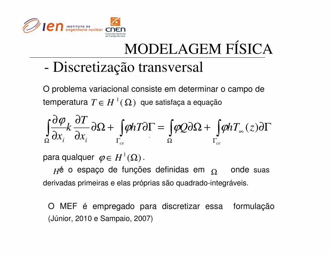
MODELAGEM FÍSICA
O problema variacional consiste em determinar o campo de
temperatura que satisfaça a equação
é o espaço de funções definidas em onde suas
derivadas primeiras e elas próprias são quadrado-integráveis.
)(1 Ω∈ HT
∫∫∫∫Γ
∞
ΩΓΩ
Γ∂+Ω∂=Γ∂+Ω∂∂
∂
∂
∂
cece
zhTQhTx
Tk
x ii
)(ϕϕϕϕ
1H
para qualquer .)(1 Ω∈ Hϕ
.
Ω
- Discretização transversal
O MEF é empregado para discretizar essa formulação (Júnior, 2010 e Sampaio, 2007)

MODELAGEM COMPUTACIONAL
Exemplos de gráficos esquemáticos de perfis de temperatura em seções transversais com a pastilha combustível concêntrica e excêntrica ao revestimento.
O software GID (interface gráfica) foi customizado para apresentar os resultados gerados pelo código VARETA_COMBUSTÍVEL.

MODELAGEM COMPUTACIONAL
- Ajuste do nível de potência
O problema de ajuste do nível de potência pode ser entendido pela pergunta: “Qual deve ser o nível máximo de potência do reator para que as temperaturas máximas do combustível e do revestimento e o DNBR mínimo alcancem os limites estabelecidos pelo projeto?”.

VALIDAÇÃO DO CÓDIGO COMPUTACIONAL
Validação do código computacional em relação à discretização axial de q’’’(z) para pastilha concêntrica ao revestimento.
A validação do código VARETA_COMBUSTÍVEL em relação àdiscretização axial de q’’’(z) para pastilha concêntrica ao revestimento foi feita comparando-se a resolução analítica de um problema apresentado e resolvido por Todreas e Kazimi (1993, p.587) com os resultados numéricos gerados por ele.

ESTUDO DE CASOSCOMPARAÇÃO DE RESULTADOS DE TEMPERATURA PARA PASTILHAS EXCÊNTRICAS AO REVESTIMENTO COM RESULTADOS DE TEMPERATURA PARA PASTILHAS CONCÊNTRICAS AO REVESTIMENTO.
Essa tabela mostra que excentricidade na pastilha combustível fez o DNBR alcançar seu limite mais rapidamente com o aumento dos níveis de potência.