Predictive Analysis on Time Series Data with

SAS

By Cho Eunwoo

Background Information

• They are about the estimates of monthly carbon dioxide emissions from fossil-fuel burning in the United States from 1981 to 2003.

• This time series dataset contains 274 observations.

• Source: http://cdiac.ornl.gov/ftp/trends/emis_mon/emis_mon_usatotal.dat

Original Time Plot

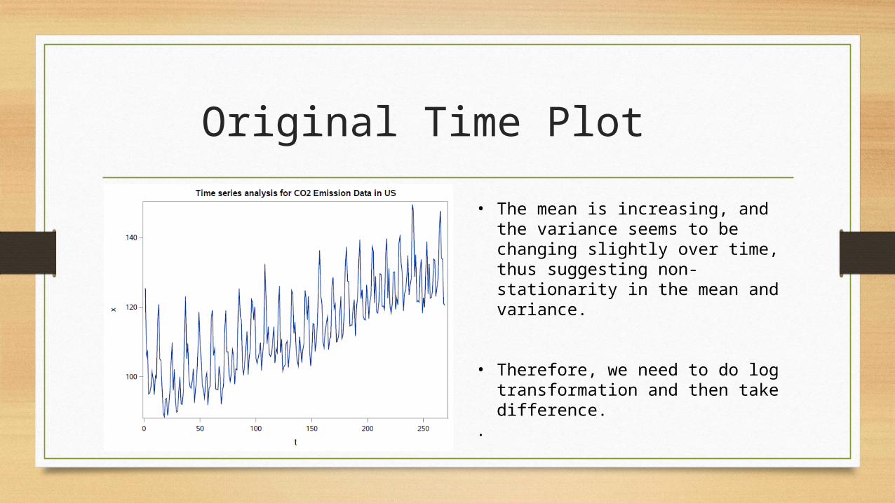
• The mean is increasing, and the variance seems to be changing slightly over time, thus suggesting non-stationarity in the mean and variance.

• Therefore, we need to do log transformation and then take difference.

.

Transformed Time Plot

Trend and Correlation Analysis

Model Specification

• Considering the nature of the data, which is monthly, and the fact that the sample ACFs are significant at lag 12 and 24, we take seasonal difference with s=12.

Model Specification

• Since it is the seasonal time series, we do not focus on PACFs as the patterns are difficult to explain except the pure seasonal AR or MA models.

• A seasonal ARIMA(0,1,0)×(0,1,1)12 model may be identified.

Model Estimation and Diagnostics

Model Estimation and Diagnostics

Forecasting

Forecasting

Ture value log(true value)

forecast of log()

95% C.I.

120.7394 4.7936 4.8124 (4.7615, 4.8633)

132.4187 4.8860 4.8738 (4.8172, 4.9305)

135.1314 4.9062 4.8850 (4.8231, 4.9469)

121.7753 4.8022 4.7979 (4.7311, 4.8647)

125.2487 4.8303 4.8276 (4.7563, 4.8989)

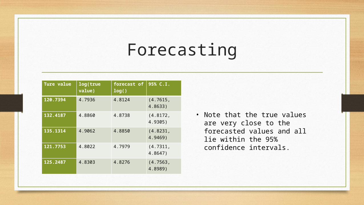
• Note that the true values are very close to the forecasted values and all lie within the 95% confidence intervals.