PREDICTION OF THE TRANSIENT FORCE SUBSEQUENT …etd.lib.metu.edu.tr/upload/12610489/index.pdf ·...

PREDICTION OF THE TRANSIENT FORCE SUBSEQUENT TO A LIQUID MASS IMPACT ON AN ELBOW

OF AN INITIALLY VOIDED LINE

A THESIS SUBMITTED TO THE GRADUTE SCHOOL OF NATURAL AND APPLIED SCIENCES

OF MIDDLE EAST TECHNICAL UNIVERSITY

BY

BÜLENT ABBAS KAYHAN

IN PARTIAL FULFILLMENT OF THE REQUIREMENTS FOR

THE DEGREE OF DOCTOR OF PHILOSOPHY IN

CIVIL ENGINEERING

FEBRUARY 2009

Approval of the thesis:

PREDICTION OF THE TRANSIENT FORCE SUBSEQUENT TO A LIQUID MASS IMPACT ON AN ELBOW


submitted by BÜLENT ABBAS KAYHAN in partial fulfillment of the requirements for the degree of Doctor of Philosophy in Civil Engineering Department, Middle East Technical University by, Prof. Dr. Canan Özgen _____________________ Dean, Graduate School of Natural and Applied Sciences Prof. Dr. Güney Özcebe _____________________ Head of Department, Civil Engineering Assoc. Prof. Dr. Zafer Bozkuş Supervisor, Civil Engineering Dept., METU _____________________ Examining Committee Members: Prof. Dr. Turgut Tokdemir _____________________ Engineering Sciences Dept., METU Assoc. Prof. Dr. Zafer Bozkuş _____________________ Civil Engineering Dept., METU Prof. Dr. Metin Ger _____________________ Civil Engineering Dept., METU Assist. Prof. Dr. Şahnaz Tiğrek _____________________ Civil Engineering Dept., METU Dr. Uğraş Baran _____________________ Havelsan A.Ş.

Date: February 27, 2009

iii

I hereby declare that all information in this document has been obtained and presented in accordance with academic rules and ethical conduct. I also declare that, as required by these rules and conduct, I have fully cited and referenced all material and results that are not original to this work. Name, Last Name: BÜLENT ABBAS KAYHAN

Signature :

iv

ABSTRACT

PREDICTION OF THE TRANSIENT FORCE SUBSEQUENT

TO A LIQUID MASS IMPACT ON AN ELBOW


Kayhan, Bülent Abbas

Ph. D., Department of Civil Engineering

Supervisor: Assoc. Prof. Dr. Zafer Bozkuş

February 2009, 263 pages

The aim of the thesis, is to find the transient force applied by an individual

transient liquid slug on an elbow at the end of a horizontal line due to an impact. The

liquid slug is driven by pressurized air in a tank located upstream of the pipeline.

The time dependent pressure distribution along the elbow and a vertical

extension segment after the elbow was solved, with a 1-D numerical approach along

a curved line mesh. For this purpose; firstly, a 3-D axial turbulent velocity profile

function was assumed for the slug, with its shape allowed to sway towards the

convex side of the elbow along the curved mesh with the aid of a calibration tool.

Then, the pressure values were calculated by using 1-D application of

Reynolds Equations in cylindrical polar and cartesian coordinates for the elbow and

the vertical extension segment, respectively. The transient force acting on the elbow

v

and the following vertical extension segment was found by using these calculated

pressure values and applying conservation of momentum principle over the volume

elements selected along the elbow and the vertical extension segment.

For the analysis of the slug motion from the pressurizer tank to the elbow, a

previously written computer code BOZKUŞ-2 was utilized. Then, the elbow and the

vertical extension segment calculations in this study were made with a new code

KAYHAN, which is an improved version of BOZKUŞ-2.

The calculated transient force and impact pressures at the elbow were also

compared with those from previous studies.

Keywords: Liquid Slug, Elbow, Turbulent Velocity Profile, BOZKUŞ-2,

KAYHAN, Transient Force

vi

ÖZ

BAŞLANGIÇTA BOŞ OLAN BİR BORU HATTININ DİRSEĞİNE

BİR SIVI KÜTLESİNİN ÇARPMASI SONUCU OLUŞAN

TRANSİT KUVVETİN TAHMİNİ

Kayhan, Bülent Abbas

Doktora, İnşaat Mühendisliği Bölümü

Tez Yöneticisi: Doç. Dr. Zafer Bozkuş

February 2009, 263 sayfa

Bu tez çalışmasının amacı yatay bir boru hattının sonundaki dirseğe çarpan

tekil bir su kütlesinin uyguladığı transit kuvvetin belirlenmesidir. Su kütlesi

membada bulunan bir tanktaki basınçlı hava tarafından itilmektedir.

Dirsekte ve ona bağlı, borunun bir düşey uzantı kısmındaki basınç dağılımın

zamana bağlı değişimi, eğrisel bir hat şeklindeki ağ üzerinde 1 boyutlu nümerik bir

yaklaşım ile çözümlenmiştir. Bu amaçla, ilk olarak 3 boyutlu bir eksenel, türbülanslı

akım hız profili fonksiyonu tahmin edilmiştir ve bu fonksiyonun şeklinin seçilen hat

üzerideki eğrisel ağ boyunca, kalibrasyon parametresi olarak kullanılan diğer bir

fonksiyon yardımı ile dirseğin konveks tarafına doğru deforme olabilmesi

sağlanmıştır.

Basınç değerleri silindirik kutupsal ve kartezyen koordinatlardaki Reynolds

vii

Denklemleri’nin, dirsek ve borunun düşey uzantı kısımlarında 1 boyutlu olarak

uygulanması ile hesaplanmıştır. Dirseğe ve ona bağlı, düşey uzantı kısmına etkiyen

transit kuvvet; hesaplanan bu basınç değerleri kullanılarak ve momentumun

korunumu prensibinin dirsek ve düşey uzantı kısmı boyunca seçilen hacimsel

elemanlar üzerinde uygulanması ile bulunmuştur.

Su kütlesinin basınç tankından dirseğe kadar olan hareketinin analizi için

daha önce yazılmış bir bilgisayar kodu olan BOZKUŞ-2 kullanılmıştır. Daha sonra

bu çalışmadaki dirsek ve düşey uzantı kısmı için olan hesaplamalar, BOZKUŞ-2’nin

geliştirilmiş bir versiyonu olan KAYHAN isimli yeni bir kod ile yapılmıştır.

Tezde, dirsekte hesaplanan darbesel basınçlar ve bulunan transit kuvvet

değerlerinin daha önce yapılan çalışmalarda bulunan sonuçlarla karşılaştırılması da

yer almaktadır.

Anahtar Kelimeler: Su kütlesi, Dirsek, Türbülanslı Akım Hız Profili,

BOZKUŞ-2, KAYHAN, Transit Kuvvet

viii

To My Parents

ix

ACKNOWLEDGEMENTS

I would like to express my deepest gratitude to my supervisor Assoc. Prof.

Dr. Zafer Bozkuş for his invaluable guidance and suggestions throughout this study.

I would like to express my special thanks also to my doctoral committee members,

Prof. Dr. Metin Ger, Prof. Dr. Turgut Tokdemir, Assist. Prof. Dr. Şahnaz Tiğrek and

Dr. Uğraş Baran for their valuable suggestions and comments.

My very special thanks extend to Assist. Prof. Dr. Özgür Kurç for his help in

providing the opportunity to use METU Central Server System as a source of

compiler software. Special thanks also go to Assist. Burak Anıl, Assist. Kaan Özenç

and Assist. İlker Küçüktepe for their assistance in the procedure of setting up the

compiler software on computer and making it ready for use.

x

TABLE OF CONTENTS

ABSTRACT …………………………………………………………………….. iv

ÖZ ……………………………………………………………………………….. vi

ACKNOWLEDGEMENTS …………………………………………………...… ix

TABLE OF CONTENTS ………………...……….……………………...….....… x

LIST OF TABLES …………………………………………………………….. xiii

LIST OF FIGURES …………………...………………………………..........… xiv

LIST OF SYMBOLS ….…...………………………………………………....... xvii

CHAPTERS

1. INTRODUCTION ……….………..……………………...…………... 1

1.1 Rationale for the Present Study …….......……………..……… 1

1.2 Specific Objectives of the Present Study …….………….…… 2

1.3 Scope of the Present Study …………………………...……… 3

2. LITERATURE REVIEW ……………………………………………... 4

3. MATHEMATICAL DEVELOPMENT FOR THE HORIZONTAL

PART ……………..…………...……………………………………... 11

3.1 Introduction ……………………………………………….... 11

3.2 Slug Dynamics Equations …………………………………... 12

3.2.1 Conservation of Mass Equation ……………..…….. 14

3.2.2 Conservation of Momentum Equation ……………. 16

3.2.3 Slug Kinematics Equation ………………………… 18

3.3 Gas Dynamics Equations ….……...………...........……….… 19

3.4 Coupling of Gas and Slug Dynamics Equations ……...…...... 21

3.5 Functional Hold Up Coefficient ……………………....….... 25

3.6 Closure ……………………………………………………… 26

4. MATHEMATICAL DEVELOPMENT FOR THE ELBOW PART … 28

4.1 Introduction …………………………………………………. 28

xi

4.2 Assumed Axial Velocity Profile Function ……….................. 29

4.3. Calculation of the Impact Pressures at the Elbow ……..…… 36

4.3.1 Simplifying Assumptions …………………….…… 38

4.3.2 Pressure Distribution Equations …………………... 44

4.3.2.1 Average Pressure Distribution along the

Vertical Extension Segment …………...... 44

4.3.2.2 Average Pressure Distribution along the

Elbow …………………………...……….. 47

4.3.2.3 Calculation of Impact Pressures at the

Convex Side of the Elbow ………………. 49

4.3.3 Calculations for that Part of the Slug in the Horizontal

Pipe ………….…………………………………….. 53

4.3.4 The Initial and the Boundary Conditions ….……… 55

4.4 Transient Force Calculations at the Elbow Part …………….. 61

4.4.1 Calculations at the Elbow ……………...………….. 62

4.4.1.1 Horizontal Transient Force Distribution

at the Elbow ………………..……….…... 63

4.4.1.2 Vertical Transient Force Distribution at

the Elbow ……………....……………….. 66

4.4.2 Calculations at the Vertical Extension Segment …... 67

4.4.2.1 Horizontal Transient Force Distribution at

the Vertical Extension Segment ………… 67

4.4.2.2 Vertical Transient Force Distribution at

the Vertical Extension Segment ……….....… 69

4.4.3 Total Horizontal and the Vertical Transient

Forces ……………………………………………... 70

4.5 Numerical Integrations ………...…………………………..... 71

4.5.1 Double Integration in Polar Coordinates ………..… 71

4.5.2 Evaluation of Numerical Line Integrals ………...… 77

4.5.2.1 Generation of 1-D Clustered Mesh …….... 77

4.5.2.2. Application of 3-Point Gauss Quadrature

Method ……………………………..…… 79

xii

4.6 Calibration Function for the Velocity Profile ………………. 81

4.7 Non-Dimensionalization of the Equations ………………..… 86

4.8 Discretization of the Equations ……………………………... 95

4.9 Evaluation of Local Peak Pressures ……………………….... 99

4.9 Input Data, Mesh Sizes and Error Analyses ……………..….. 99

4.10 Neglecting of Some Terms ……………………………….. 100

4.11 Input Data, Mesh Sizes and Error Analyses ……………… 104

4.11.1 Input Data for Program KAYHAN …………….. 104

4.11.2 Error Analysis and Mesh Size for Area

Integrals ……………………………………...… 106

4.11.3 Error Analysis and Mesh Size for Line

Integrals ………………………………………... 110

4.11.4 Mesh Size and Error Analysis for the Line Mesh along

s -Curve ………………………………………….. 112

4.11.5 Error Analysis and the Mesh Size for Impact Pressure

Calculation …………..………………………….. 115

5. RESULTS AND DISCUSSION ……………………………………. 117

5.1 Peak Pressures at the Elbow ……………………………….. 118

5.2 Pressure-Time History Plots ……………………………….. 120

5.3 Transient Forces at the Elbow ……………………………... 129

5.4 Impact Pressure Distribution at the Elbow ………………… 137

5.5 Discussion on the Existence of Waterhammer Event ……… 140

6. CONCLUSIONS ……………………………………………………. 142

6.1 Summary …………………………………………………... 142

6.2 Concluding Remarks ………………………………………. 143

REFERENCES …………………………………………………………...…… 145

APPENDICES

A. MATHEMATICAL DERIVATION OF THE EQUATIONS …....... 150

A.1 Functional Hold up Coefficient Determination …………… 150

A.1.1 Formulation for the Average Slug Length ………. 150

A.1.2 Correlation between the Hold up and the

Instantaneous Slug Length ……………………... 152

xiii

A.2 Derivations for the Assumed Velocity Profile Function ….. 151

A.2.1 Derivation of Bottom Cone Equation …………… 151

A.2.2 Derivation of Upper Cone Equation …………….. 158

A.2.3 Calculation of Unknown Parameters ……………. 160

A.3 Derivations for the Pressure Distribution Equations ……… 165

A.3.1 Derivation of Average Pressure Distribution

Equation at the Vertical Extension Segment …..... 165

A.3.2 Derivation of Average Pressure Distribution

Equation at the Elbow ……………....…………... 170

A.3.3 Derivation of the Equation for the Pressure at the

Convex Side of the Elbow ……………………… 179

A.4 Derivations for the Transient Force Calculations at the

Elbow Part ………………………………………………… 184

A.4.1 Derivations for the Horizontal Transient Force

Distribution at the Elbow ……………………...... 184

A.4.2 Derivations for the Vertical Transient Force

Distribution at the Elbow ……………………… 188

A.4.3 Derivations for the Horizontal Transient Force

Distribution at the Vertical Extension Segment … 191

A.4.4 Derivations for the Vertical Transient Force

Distribution at the Vertical Extension Segment … 194

A.5 Derivations for Numerical Integration Formulas …………. 196

A.5.1 Derivations for Double Integrals in Polar

Coordinates ……………………………………... 196

A.5.2 Derivations for the Line Integrals ……………….. 200

A.5.2.1 Derivations for 1-D Clustered Mesh

Generation ……………………………... 201

A.5.2.2 Derivations for 3-Point Gauss

Quadrature Method ……………………. 202

A.6 Derivations for the Calibration Function ………………….. 205

xiv

B. CORRELATION FUNCTION FOR THE MAXIMUM

CALIBRATION ANGLE ………………………………………….. 206

C. COMPUTER PROGRAMS ………………………………………... 213

C.1 Explanations for the Functions of the Computer

Programs …………………………………………………... 213

C.2 Flow-Chart for the Computer Code KAYHAN …………... 218

C.3 Computer Code KAYHAN ……………………………….. 224

xv

LIST OF TABLES

TABLES Table 4.1 Initial and the boundary conditions for the elbow and the vertical extension segment calculations. ………….............................…….………. 58 Table 4.2 Values for the terms in Equation (4.81). ……………………………. 100 Table 4.3 Values for the terms in Equation (4.85). ……………………………. 101 Table 4.4 Radial and axial velocities with their time derivatives. ……………... 103

Table 4.5 Input data for program KAYHAN. …………………………………. 105 Table 5.1 Peak pressures at the elbow (psig). …………………………………. 101 Table A.1 Calculation steps for avep LL / ( .4488.9 mLp ). …………...……... 154 Table B.1. Peak pressures used for correlating maxc (all in psig). …………... 207 Table B.2 maxc values vs. inp L/L used for correlation procedure. ………….. 211

xvi

LIST OF FIGURES

FIGURES Figure 2.1 Fenton’s experimental setup [22]. ………...………..……………...… 5 Figure 2.2 System setup used in Bozkuş’s study [2]. …………………………... 6 Figure 2.3 Experimental setup used by Baran [27]. …………………………….. 9 Figure 3.1 Control volume for the liquid slug selected by Bozkuş [2] along the horizontal pipeline. ………………….……………………………………. 13 Figure 3.2 Computational domain used by Bozkuş [2] for the solution of gas dynamics equations. ……………………………………………………… 21

Figure 3.3 Variation of pressure at the upstream pressure tank (Bozkuş [2]). ..... 25 Figure 4.1 Velocity distribution in a curved pipe given by Prandtl [13], [14] (Schlichting [10]). ………………………………………………………... 29 Figure 4.2 Parameters for the general oblique cone equation. ………………….. 30 Figure 4.3 Cross-sectional shape of the assumed turbulent velocity profile function. ………………………………………………………………….. 32 Figure 4.4 Parameters used for the assumed velocity profile in a single coordinate system. ………………………………………………………... 33 Figure 4.5 (a) Complete physical set up for the system (Bozkuş [2]); Computational domain for (b) the elbow and the vertical extension part, (c) the cross-section of the elbow, (d) the cross-section of vertical extension part of the pipe. ……………………………………………….. 34 Figure 4.6 Sample volumetric pipe element on the s-curve, in the vertical extension segment. ………………………………………………. 45 Figure 4.7 Sample volumetric pipe element along the s-curve, for the elbow part. ………………………………………………………………………. 48 Figure 4.8 1-D radial mesh at a cross-section of the elbow. ……………………. 50 Figure 4.9 1-D radial mesh selection at elbow cross-sections, with the line meshes located in the vertical, mid yx plane of the elbow. …………... 52

xvii

Figure 4.10 Computational domain with the nodal numbering along the s -curve given. ………..…………………………………………………... 56 Figure 4.11 Control volume for the transient force calculations at the elbow. …. 62 Figure 4.12 Selection for the location of the P values along the s -curve, for the procedure of interpolation at the faces of the volume elements. ……….... 65 Figure 4.13 Control volume for the transient force calculations at the vertical extension segment. ………………………………………………….. 68 Figure 4.14 Circular mesh over the pipe cross-section. ………………………… 72 Figure 4.15 9-point mesh element selected for double integration in polar coordinates. ………………………………………………………………. 74 Figure 4.16 9-point mesh element for 2-D Gauss Quadrature in cartesian coordinates. ………………………………………………………………. 75 Figure 4.17 Mesh element for the center point of the circular domain in polar coordinates. ……………………………………………………………… 76 Figure 4.18 Line mesh for a given point K on the elbow cross-section. ………. 78 Figure 4.19 Parameters used for the 3-point Gauss Quadrature Method. ………. 80 Figure 4.20 Shape of the calibration function c . ……………………………… 82 Figure 4.21 General variation of the shape of the assumed axial velocity profile along the s –curve. ………………………………………………………. 85 Figure 4.22 Percentage error vs. total mesh size, for 10.mrt ………………. 107 Figure 4.23 Percentage error vs. total mesh size, for 250.mrt ……….…….. 108 Figure 4.24 Percentage error vs. total mesh size, for 50.mrt ………………. 108 Figure 4.25 Percentage error vs. total mesh size, for 750.mrt ……………... 109 Figure 4.26 Percentage error vs. total mesh size, for 01.mrt ………………. 109 Figure 4.27 Percentage error vs. total mesh size, for 51.mrt ………………. 110 Figure 4.28 Variation of percentage error vs. node number, LM . ……………. 112 Figure 4.29 Variation of percentage error vs. node number, slugN …………….. 115

xviii

Figure 5.1 Normalized peak pressures vs. inp L/L . …………………………... 119

Figure 5.2 Pressure-time history plots at the elbow for 4inL ft and 200 P psig. .…………………………………………………………..... 123

Figure 5.3 Pressure-time history plots at the elbow for 4inL ft and 300 P psig. .………………………………………………………….... 123

Figure 5.4 Pressure-time history plots at the elbow for 4inL ft and

400 P psig. .……………………...……………………………………. 124

Figure 5.5 Pressure-time history plots at the elbow for 5inL ft and 100 P psig. .………………………………………………………...….. 124

Figure 5.6 Pressure-time history plots at the elbow for 7inL ft and 100 P psig. .……………………………………………………………. 125


200 P psig. .……………………………………………………………. 125 Figure 5.8 Pressure-time history plots at the elbow for 7inL ft and

400 P psig. .…...……………………………………………………….. 126

Figure 5.9 Pressure-time history plots at the elbow for 9inL ft and 100 P psig. .………...………………………………………………….. 126

Figure 5.10 Pressure-time history plots at the elbow for 11inL ft and 100 P psig. .…...……………………………………………………….. 127


200 P psig. .…...……………………………………………………….. 127

Figure 5.12 Pressure-time history plots at the elbow for 11inL ft and 300 P psig. .……...…………………………………………………….. 128

Figure 5.13 Pressure-time history plots at the elbow for 11inL ft and 400 P psig. .……………………………………………………...…...… 128

Figure 5.14 Transient force components for 4inL ft and 100 P psig. ..…... 130 Figure 5.15 Transient force components for 4inL ft and 200 P psig. ..….. 130

xix

Figure 5.16 Transient force components for 7inL ft and 100 P psig. ..…... 131 Figure 5.17 Transient force components for 7inL ft and 200 P psig. ..….. 131 Figure 5.18 Transient force components for 11inL ft and 200 P psig. ..…. 132 Figure 5.19 Transient force components for 11inL ft and 400 P psig. ..…. 132 Figure 5.20 Values of *F vs. *D (Bozkuş’s [2] 1st peaks were used for normalization). ………………………………………………………….. 134 Figure 5.21 Values of *F vs. *D (Bozkuş’s [2] 2nd peaks were used for normalization). ………………………………………………………….. 136 Figure 5.22 Dynamic pressure distribution for inL 4 ft, 0P 20 psi,

t 0.539 s and NELBW 115. .………………………………………... 138

Figure 5.23 Dynamic pressure distribution for inL 4 ft, 0P 40 psi, t 0.375 s and NELBW 115. ..………………………………………... 138

Figure 5.24 Dynamic pressure distribution for inL 7 ft, 0P 10 psi, t 0.942 s and NELBW 90. .…………………………………………. 139

Figure A.1 Normalized peak pressures vs. inp LL / from program BOZKUŞ-2 and from the experimental data (Bozkuş [2]). ………………………….. 153 Figure A.2 Variation of hold up coefficient, , as a function of sp LL / . ……. 155 Figure A.3 Two coordinate systems combined together for the general oblique and symmetric cone equations. …………………………………………. 156 Figure A.4 Control volume at the elbow with the components of the forces and the velocities shown. ……………………………………………….. 185 Figure B.1 Normalized peak pressures at the elbow for maxc 89.60°. ……… 208 Figure B.2 Normalized peak pressures at the elbow for maxc 89.70°. ……… 208 Figure B.3 Normalized peak pressures at the elbow for maxc 89.75°. ……… 209 Figure B.4 Normalized peak pressures at the elbow for maxc 89.77°. ……… 209 Figure B.5 Normalized peak pressures at the elbow for maxc 89.80°. ……… 210

xx

Figure B.6 Normalized peak pressures at the elbow for maxc 89.82°. ……… 210 Figure B.7 Correlation function for maxc vs. inp L/L . ……………………….. 212

xxi

LIST OF SYMBOLS

a : wave speed,

a : coordinate axis used as the transformation parameter,

A : cross-sectional area of the pipeline, elbow and the vertical extension

segment,

1A , 2A : areas of the parts of the pipe cross-section,

3A , 4A : outer surface areas of the infinitesimal volume element

perpendicular to pipe axis and the at the pipe wall; respectively,

A : lower boundary of the line integral,

cA , cB : points on the coordinate system for the calibration function, c ,

*tA , *A : differential expression,

*tB : differential expression,

C : wave speed,

C : control volume,

CS : control surface,

1C , 2C : parameters,

rc : mesh clustering ratio used for the line mesh,

D : pipe diameter, *D : dispersion distance,

E : integral expression, *

1E , *2E , *E3 : parameters,

f : integrand function,

ff : friction factor,

fwf : friction factor for water,

xxii

F : friction force per unit length of the pipe assuming no reverse flow,

F

: force vector acting on the control volume,

mF : predicted force at the elbow with the numerical model,

pF : experimentally obtained peak force at the elbow,

vecF

: vectorial expression,

xF : force acting on the volumetric element in x -direction,

xF , yF : x and y components of the total transient force acting on the

elbow and the vertical extension segment, respectively,

yF : force acting on the volumetric element in y -direction,

*F : normalized force,

g : gravitational acceleration,

xg , yg , zg : components of gravitational acceleration respectively in x , y

and z directions,

rg , g : components of gravitational acceleration respectively in r and

directions,

g : functional parameter as integrand,

ig , cig : parameters having discrete values at points i ,

1h , 2h , 3h : parameters for the geometry of the velocity profile function,

h : any integrand function for the line integral,

1h , 2h , 3h : values of the function h over the nodes of the 1-D Gauss

element,

i , j , k : incremental grid location in r , and z directions, respectively,

ip : indice for the node number,

AI : area integral expression,

nmAI ,; : expression for the area integral over the mesh element in the circular

domain A , with the mesh element’s center point at node nm, ;

nmAcI ,; : expression for the area integral over the central mesh element in the

circular domain A , with the mesh element’s center point at node nm, ;

xxiii

LI : line integral expression,

1LI : integral expression,

qLI , : expression for the line integral over the line mesh element with the

mesh elements’s center point located at node q ,

*uI , *

I , *usI : integral expressions,

mK : minor loss coefficient at the elbow,

K : upper boundary of the line integral,

l : mixing length,

ml : mixing length,

L : slug length remaining within the horizontal part of the pipeline,

L : scaling factor for length,

aveL : average length of the slug that occurs during the motion of the slug

along the horizontal part of the pipeline,

elbL : central arc length of the elbow,

extL : length of the vertical extension segment after the elbow,

finL : final slug length of the horizontal pipe calculations ,

finalL : final length of the slug remaining in the horizontal part of the pipeline

obtained from horizontal pipe calculations,

inL : initial slug length,

pL : length of the horizontal part of the pipeline,

sL : instantaneous slug length at any time during its travel along the

horizontal part of the pipeline,

impsL : slug length at the instant that the slug front enters the elbow,

tL : travel distance of the slug,

totL : total axial length of the elbow and the vertical extension segment,

m : indice for the radial location of the mesh element in the circular domain,

M and N : number of mesh elements in the radial and the circumferential

directions of the pipe cross-section, respectively,

xxiv

MLPRSS : number of nodes for the line mesh used for the impact pressure

calculation,

LM : total number of clustered line mesh elements in case the domain of line

integral is the whole diameter of the cross-section of the elbow, in r direction,

rtm : Ratio of the circumferential mesh size to the radial one, at any cross-

section of the pipe,

1cm , 2cm : slopes of the calibration function, c , before and after its point

of maximum, respectively,

n : indice for the circumferential location of the mesh element circular

domain,

NBOUND : point on the s -curve at the boundary of the elbow and the

vertical extension segment,

NELBW : number of nodes along the axis of the elbow,

NLFF : nodal number corresponding to the location of the slug front face

along the s -curve,

slugN : number of nodes selected over the slug length, impsL .

NSTOT : total number of nodal points along the s -curve,

ktanN : number of tank pressure data points,

n : outer unit normal vector,

O : center of curvature of the elbow,

O : origin of the local coordinate system,

O : origin of the upper local coordinate system,

cO : origin of the coordinate system for the calibration function, c ,

p : ensemble average local pressure,

P : average pressure over the pipe cross-section,

calcP : calculated average pressure value at the elbow cross-section,

DP : driving air pressure acting on the slug upstream face,

finalDP : final driving air pressure value at the upstream face of the slug from

horizontal pipe calculations at the instant that the slug front face reaches the entrance

section of the elbow,

xxv

EP : average liquid pressure retarding the motion of that part of the slug in

the horizontal part of the pipeline, and acting at the entrance section of the elbow,

calcEP : calculated average liquid pressure retarding the motion of that part of

the slug in the horizontal part of the pipeline, and acting at the entrance section of the

elbow,

0P : initial tank pressure at the pressurizer tank,

atmP : atmospheric absolute pressure,

dP : average pressure acting at the downstream face of the control volume,

NLFFP : atmospheric pressure at the front face of the liquid slug,

NBOUNDP : average pressure at the connection boundary of the elbow and the


Op : local pressure at the center point O of the elbow cross-section,

pP , mP and nP : average pressures at the center points of respectively the

previous, current and next volume elements on the s -curve,

peakp : peak pressure from program KAYHAN at the location of transducer

#2.

TP : tank pressure,

finalTP : final tank pressure value from horizontal pipe calculations at the

instant that the slug front face reaches the entrance section of the elbow,

uP : average pressure acting at the upstream face of the control volume,

wP : driving air absolute pressure acting at the upstream face of the slug,

wetP : wetted perimeter,

PO : atmospheric pressure,

gagePO : atmospheric gage pressure,

q : any node number of the line mesh, also coinciding with the center point

of a 1-D Gauss element,

Q : discharge,

KQ : mesh size of the 1-D clustered line mesh,

xxvi

r : radial axis of the cylindrical coordinate system,

R : internal radius of the pipe,

R : radius of the bottom circle of the lower cone,

R : radius of the bottom circle of the upper cone,

Re : Reynolds number,

RHS : right-hand side of equation,

gR : gas constant,

0R : radius of curvature of the elbow,

mr : given radial coordinate in the cross-section of the elbow, with respect to

the cylindrical coordinate system,

mR : distance of the point of maximum velocity from the origin of the local

coordinate system, measured along the y axis,

qr : radial location of the center point of the 1-D Gauss element over the

clustered mesh, with respect to the cylindrical coordinate system,

s : curvilinear coordinate,

S : surface area of the control volume,

dS : downstream pipe cross-sectional area for the control volume,

ds , us : location of respectively the downstream and the upstream faces of

the current volume element at node ip , on the s -curve,

elbs : location on s -curve for the exit section of the elbow,

exts : location on s -curve for the exit section of the vertical extension

segment,

mS : area of the mid-plane of the volume element perpendicular to pipe axis,

maxs : location on s -curve where the maximum value of c occurs,

ps , ms , ns : location of the center points of respectively the previous, current

and next volume elements on the s -curve,

uS : upstream pipe cross-sectional area for the control volume,

nfrols : slug front face location on the s -curve at ant time step n ,

s , t : cartesian axes as parameters for coordinate transformation,

xxvii

t : time,

T : temperature,

t : scaling factor for time,

int : initial time of slug motion,

fint : final time of slug motion,

nt : time value at any time step n ,

U : average slug velocity,

U : scaling factor for velocity,

aveU : average velocity of the slug taken over the cross-section of the elbow,

bU

: velocity of the boundary of the control surface,

BU : velocity of the back face of the slug,

finalU : final slug velocity obtained from horizontal pipe calculations,

FU : velocity of the front face of the slug,

inU : initial slug velocity,

ixU : fluid velocity relative to the global coordinate axis, on the surface i for

the control volume, and in the x -direction,

mU : maximum velocity on the assumed velocity profile function,

pasU : slug passage velocity through the elbow,

rU

: liquid velocity relative to the control surface boundary,

riU : fluid velocity relative to the control surface i ,

su : velocity profile function defined along the s-curve,

suu , sdu : axial velocity profile functions at the upstream and the downstream

faces of the volume element,

su : average value of the assumed axial velocity profile function along the s -

curve,

xU : liquid velocity relative to the fixed reference frame,

u : axial velocity profile function in the elbow, in direction,

u : average value of the velocity profile function in the elbow, in

xxviii

direction,

uu , du : assumed and calibrated axial velocity profile functions evaluated at

respectively the upstream and downstream faces of the control volume,

V : velocity within the air volume, in the x -direction,

axialV : axial velocity,

V

: velocity vector at any point of the flow,

rV , V : ensemble average local velocity components respectively in r and

directions,

rV , V : turbulence fluctuations of the velocity components respectively in r

and directions,

rdV : local radial velocity at the downstream face of the control volume,

ruV : local radial velocity at the upstream face of the control volume,

xV , yV , zV : ensemble average local velocities respectively in x , y and z

directions,

xV , yV , zV : turbulence fluctuations of the velocity components respectively

in x , y and z directions,

xdV : local velocity in x -direction at the downstream face of the control

volume,

xuV : local velocity in x -direction at the upstream face of the control volume,

yV : average velocity in y direction,

yuV , ydV : local velocities in y -direction at respectively the upstream and the

downstream faces of the control volume,

dV : local axial velocity at the downstream face of the control volume,

uV : local axial velocity at the upstream face of the control volume,

V : average axial velocity in -direction,

1w , 2w , 3w : weighting coefficients,

x , y : cartesian coordinate axes,

x , y , z : coordinate axes for the local coordinate system,

xxix

x , y , z : coordinate axes for the upper local coordinate system,

inX : initial slug position,

0x , 0y , 0z : coordinates for the apex point of the general cone equation,

0x , 0y , 0z : coordinates for the apex point of the upper cone with respect to

the upper local coordinate system,

wy : distance from the pipe wall,

1y , 2y : parameters for the geometry of the velocity profile function,

z : axis of the cylindrical polar coordinate axes,

nz : given z coordinate in the cross-section of the elbow, with respect to the

cylindrical coordinate system.

Greek symbols:

: hold up coefficient,

: angular axis,

d : reference angle for the downstream face of the control volume,

u : reference angle for the upstream face of the control volume,

p : circumferential coordinate for the given cross-section of the elbow , with

respect to the cylindrical coordinate system,

xF , yF : horizontal and the vertical components of the reaction force

applied by the pipe on the control volume, respectively,

sL : whole change in slug length during the travel of the slug from the

pressurizer tank up to the elbow,

WHP : pressure rise due to sudden valve closure,

qr : length of the clustered line mesh element at node q ,

s : axial length of the volume element,

t , 1t , 2t : time increments for the horizontal pipe calculations,

past : slug passage time through the elbow,

st : time increment at any time step of the elbow and the vertical extension

xxx

segment calculations,

1st : first time increment value used for the elbow and the vertical extension

segment calculations, n

st : time increment at any time step, n ,

U : change in slug velocity,

W : weight of the control volume,

: incremental angle of curvature over the infinitesimal element in the

elbow,

: incremental angle of the mesh in direction (angular direction),

: incremental length of the mesh in direction (radial direction),

: volume of the selected pipe element,

: divergence operator,

: roughness height of the pipe wall,

t : turbulent eddy viscosity of the liquid,

: radial coordinate axis over the pipe cross-section,

m : radial distance of the central node of the 9-point mesh element from the

center-point of the domain of the circular cross-section,

: circumferential coordinate axis over the pipe cross-section,

n : angular distance between the line connecting the central node of the 9-

point mesh element to the origin of the circular domain, and the x axis,

: dynamic viscosity of water,

: pi number,

: kinematic viscosity of the liquid,

: density of the liquid (water),

a : density of air,

w : density of water,

: circumferential axis of the cylindrical polar coordinate system,

c : calibration function for the angle at a selected point of the velocity

profile function,

xxxi

entc : c value at the entrance section of the elbow,

extc : c value at the exit section of the vertical extension segment,

maxc : maximum value of c along the s -curve,

f : angle for the gradient of the velocity profile at the pipe wall,

: shear stress value at wy distance away from the circular pipe wall,

0 : wall shear stress,

: divergence operator,

: volume of the control volume,

r : volume of the volumetric element,

1 : volume of the bottom cone,

2 : volume of the oblique upper cone,

: symbol indicating ensemble averaging.

Subscripts:

ip : variable at this node

L : location of the left boundary of the gas volume,

R : location of the right boundary of the gas volume,

S : location of the right at the mid-time step.

Superscripts:

n : time level,

* : dimensionless parameter.

1

CHAPTER I

INTRODUCTION

1.1 Rationale for the Present Study

Study of the impact pressures applied by high pressure air or steam driven

liquid pockets, called slugs, formed in voided lines is an important phenomenon as

far as the resulting potential damage on the pipelines is concerned. There are some

different mechanisms that cause formation of speed motion of liquid slugs in nuclear

power plants.

One of these mechanisms is the creation of a condensate in steam lines of a

power plant during its operation, and following motion of this condensate in the form

of a liquid slug along a voided line (Kim [17]; Merilo and et al. [18]; Bozkuş and

Wiggert [20]). Inadequate draining is one of the factors that yields the formation of

condensate in a steam line which afterwards under the pushing effect of high

pressure steam may accelerate along the voided line, and turn into a slug as a whole

liquid pocket filling all the pipe cross-section during its motion. Then, the liquid slug

which attains very high speeds along the pipeline may hit elbows, partially or fully

open valves or junctions applying very high impact pressures on these parts of the

pipeline.

Another cause of slug creation in voided lines is the pushing effect of high

pressure steam on water, collected in loop seal parts of the pipelines in power plants

(Bozkuş [2]; Wheeler and Siegel [19]; Bozkuş and Wiggert [20]). A loop seal is that

part of a pressurized water reactor which is located upstream the pressurizer safety

and relief valves and it is used for preventing excessive gas leakage through these

valves. When the upstream pressure in the reactor coolant system exceeds a

previously defined limiting value, the safety or relief valves suddenly open to relieve

2

the excess pressure in the system. As soon as the valves open, the high pressure

steam starts to push the water in the loop seal causing the formation of a liquid slug

which attains very high velocities in the pipeline and applies high dynamic pressures

on such pipe components as elbows, tees and valves as a source of potential damage.

The parameters to describe the hydraulic properties of the slug motion and the

following impact event consist of initial mass and length of the slug, magnitude of

the driving pressure acting on the upstream face of the slug, pipe material and pipe

geometry. These hydraulic parameters are all effective in the value that the

magnitude of the dynamic pressures on the pipe components will reach. Since the

magnitude of the dynamic loads acting on the pipeline and its supports is a measure

of the possible damage that the pipeline system will experience, a hydrodynamic

analysis is essential to predict and mitigate any potential risk of damage to the

pipeline system. This field of hydrodynamics that analyses the forces applied by

propelled liquid slugs in voided lines is actually a subject on which a limited number

of studies were have been performed so far and this makes the subject an issue that

requires more attention. Also considering that pipeline systems and pipe supports and

restraints constitute quite a large amount of the total investments to be made for

nuclear power plants, prediction of the forces acting on these support and restraint

structures becomes an important subject of research (Bozkuş [2]; Smith and Van

Laan [21]).

1.2 Specific Objectives of the Present Study

In previously performed numerical studies related with estimation of impact

pressures and dynamic loads applied by liquid slugs on elbows of initially voided

lines, different 1-D mathematical models were proposed for the simulation of slug

motion along straight pipelines and following impact events at elbows located at the

end of the pipelines. Although these 1-D mathematical models were adequate enough

to describe the actual flow conditions for the slug motion along straight pipelines,

they have not included a much detailed modeling of elbow part calculations up to

now. Actually, differing from case for the motion of a liquid slug along a straight

part of a pipeline, the asymmetric axial velocity profile of a slug in an elbow part

requires special attention to consider that distorted profile in a numerical model.

3

The aim of the present study is to predict numerically the transient force

acting on a 90° degree elbow with its axis extending in the vertical plane, and on a

following vertical extension segment, subsequent to a liquid mass impact on those

parts. In the study, both of the elbow and the following vertical extension segment

were taken to be located at the end of a straight and initially voided pipeline

extending in the horizontal plane. For the part of the calculations that accounts for

the motion of the liquid slug in the horizontal pipeline, a previous 1-D study

performed by Bozkuş and Wiggert [2, 20] that contains gas and slug dynamics

equations were utilized. And for the elbow and the following vertical extension

segment calculations, a new 1-D analysis was performed with the intention of

making a more detailed consideration of the flow in those parts, and by taking into

account the variation of 3-D shape of the asymmetric axial velocity profile along the

elbow and the vertical extension segment.

1.3 Scope of the Present Study

In the present study, the transient force acting on a 90° elbow and the

following vertical extension segment was calculated by making a 1-D numerical

analysis. For the analysis, a calibration technique was adopted to determine the

unknown parameters for the change in the shape of an assumed 3-D axial velocity

profile along the elbow and the vertical extension segment. For the calibration

purposes, some experimental data of peak pressures obtained previously by Bozkuş

[2] were utilized as reference values. By using the calibration function obtained from

correlated data, various computer runs were made with different initial slug lengths

and initial tank pressures to get a set of plots for the peak pressure time histories at

the elbow and the time histories for the transient forces acting on the elbow and the

vertical extension segment. The obtained results for the pressure peaks, and impact

pressure and transient force time history plots were also compared with those from

previously made studies.

4

CHAPTER II

LITERATURE REVIEW

There are various studies performed by different researchers, related with the

prediction of forces that arise due to impact of a liquid slug on an elbow of an

initially voided pipeline, but the number of these works is not quite high. Those of

them which are most relevant to the present study were carried out by Woo and

Papadakis [23], Fenton [22], Bozkuş [2], Neumann and Griffith [24], Baran [27].

Woo and Papadakis [23] developed a mathematical model for the

determination of hydrodynamic forces at pipe bends that arise while an initially

voided pipeline system was being filled. In that study, a combination of rigid column

theory and method of characteristics was utilized for the mathematical modeling. As

a result of the analysis, discharges, and forces at the pipes and pipe bends calculated

with that model were seemed to be smaller than those in a previous made model by

Papadakis and Hollingshead [37]. The reason for this reduction was attributed to the

fact that in the previously made model, minor head losses at pipe junctions and pipe

bends had been neglected; and therefore, it was indicated that the inclusion of minor

losses became important if the velocities in the system were high [2, 23].

Fenton [22] performed both an analytical and an experimental study with the

purpose of predicting the forces at a pipe bend, induced by the impact of a liquid slug

which was driven by air along a pipeline. The aim of the analytical study was to

develop a simple method for the prediction of loads acting on the pipe supports. And,

an experimental work was performed to check the validity of the analytical method

developed in the same study. For this purpose, he used an experimental apparatus as

shown in Figure 2.1.

5

Figure 2.1 Fenton’s experimental setup [22].

The experimental apparatus was composed of an air pressurizer vessel to

supply high pressure air to the system and a 2-inch-diameter steel pipe was

connected to this vessel. There was ball valve at the entrance of the steel pipe to

control air flow to the system, and an orifice and a pressure transducer were also

attached to the steel pipe. At the downstream side, a 1-inch-diameter plexiglass pipe

which was inclined upwards was connected to the steel pipe. The connection here

was made by means of a Tee section which was also utilized for the purpose of

filling and draining water to the lower part of the plexiglass pipe. There was an

elbow located at the downstream end of the plexiglass pipe, which was open to the

atmosphere.

Fenton carried out his experiments with different initial slug lengths, initial

tank pressures, and also by varying the distance between the slug front face and the

elbow at the downstream side.

Fenton’s analytical model included some assumptions, the most restrictive of

which was that the slug as a coherent mass. Due to this coherent mass assumption,

6

amount of liquid that was left behind during the slug motion was neglected. As other

assumptions, the gas from the pressure vessel, driving the liquid slug was taken to be

compressed isothermally and as ideal, and the slug flow was considered as

incompressible. During the flow of gas and the liquid slug, the shear resistance acting

on the flow at the pipe wall was taken into consideration.

Fenton’s analytical study overestimated the impact loads at the elbow

especially when the normalized slug travel distance was equal to or greater than 7 [2,

22].

Bozkuş [2] performed an experimental study together with an analytical

modeling to investigate the hydrodynamics of a transient liquid mass driven by high

pressure air in a voided line. For this purpose, he used an experimental setup which

consisted of a pressurizer and a horizontal pipeline connected to this pressurizer, and

at the downstream end of the pipeline there was a 90° elbow attached together with a

vertical extension segment, as shown in Figure 2.2. There was also a slug generator

Figure 2.2 System setup used in Bozkuş’s study [2].

pipe (SGP) located between the pressurizer and a PVC ball valve. By selecting a

SGP of any desired length and filling it with water, it was possible to generate slugs

with different initial lengths. With this system setup, liquid slugs with various initial

Pressure Gauge

Pressurized Air Tank

SGP

2-inch inside diameter 31 ft. (9.45 m.)-long Clear PVC Pipe Elbow

PVCBall Valve

Transducer # 1

Transducer # 2

2 ft.

5 ft.

Accelerometer

7

lengths and under the propelling effect of different initial tank pressures were driven

along the horizontal and initially empty pipeline and the pressure time histories that

form due to impact of the liquid slugs on the elbow were recorded by the transducers

mounted on the elbow as shown in Figure 2.2. As a result of the analysis it was

concluded that long slugs lost more amount of their initial masses than did the short

slugs during their motion along the horizontal pipeline. In addition, for long and

medium slugs, two different peak pressures were observed in the pressure recordings

with respect to time at the elbow. The reason for the occurrence of this double peak

phenomenon was attributed to the disintegration of the slug mass into two pieces

following the sudden opening of the ball valve upstream. Another conclusion drawn

in this study was that more air entrainment effect was observed in the cases of short

slugs than compared to long slugs and this difference between the two cases was

explained with the reason that short slugs had a longer normalized travel distance. It

was also indicated in that study that large amounts of air entrainment was a factor

that caused significant reduction in the densities of especially short liquid slugs.

Analytical study of Bozkuş [2] consisted of two different mathematical

models. The first one of these models, called “Simple Model” [2], included two

different control volume analyses; one for the determination of peak pressures at the

elbow and another for obtaining pressure time history plots for the variation of

impact pressures at the elbow. The second mathematical model was called the

“Advanced Model” [2] and in this model, in addition to the slug dynamics equations

that was used in the Simple Model, another set of equations that also takes into

account the gas dynamics effects were included as a further improvement. The peak

pressures at the elbow were also calculated with this advanced model. Both of the

analytical models gave the peak pressures at the elbow induced by the short slugs as

being higher than the experimentally obtained ones. This overestimation of the

analytical models was indicated to be due to the fact that the air entrainment effect

was neglected in these models, which was a phenomenon that caused the density of

the liquid slug to reduce and thus, the experimentally obtained impact pressures to

become smaller as compared to those from the analytical models. The analytically

obtained peak pressures for long and medium slugs were stated to match closely with

the experimental results. A detailed explanation for the Advanced Model of Bozkuş

8

[2] is given in Chapter III together with the analytical methods followed in writing

the computer codes with both the Simple Model and the Advanced Model.

Bozkuş, et. al [20] published the findings of the study by comparing them to

those from Fenton and Griffith [26] and it was stated that the normalized forces in

Bozkuş’s experimental study were nearly the same as those given by Fenton and

Griffith except that the results from Bozkuş’s study showed a variation of data over a

relatively larger range of normalized force values. This discrepancy between the two

results was indicated to be probably due to the differences in the experimental setups

used. For example, it was pointed out that the pipe diameter in Bozkuş’s study was

twice as large as the one in the case of Fenton and Griffith’s study. In addition, it

was expressed that the pipe in Bozkuş’s study was horizontal rather than the pipe

inclined upwards pipe towards downstream that was used in the study of Fenton and

Griffith. Furthermore, it was stated that in Bozkuş’s study, a ball valve was used to

control the motion of the slug; however, Fenton and Griffith utilized a ruptured disk

for the same purpose. In conclusion, Bozkuş and Wiggert [20] suggested that these

differences between the experimental setups were likely to be the reason for higher

scatter of data in Bozkuş’s study as compared to the values obtained by Fenton and

Griffith.

Neumann and Griffith [24] studied how the forces acting on a 90° bend are

affected if the bend is located downstream of a pipe expansion. As a result of an

analysis by conducting a set of experiments it was concluded that the peak forces at a

bend located after an expansion were very close to those that occurred in case of a

pipe with a constant diameter. Another conclusion reached in that study was that for

both types of the pipes considered, the slug traveling distances required for the force

at the pipe bend to reduce to very small values were nearly the same.

Baran also [27] carried out an experimental and numerical study to

investigate the hydrodynamics of an individual transient liquid mass in voided line.

Baran’s experimental setup consisted of an air tank and a pipeline which was

inclined upward towards downstream, and this pipeline was connected to an air tank

at its upstream end through a ball valve as shown in Figure 2.3. There was a

9

Figure 2.3 Experimental setup used by Baran [27].

sharp turn elbow connected to the downstream end of the inclined pipeline, which

was extending downwards in the vertical plane. A transducer was located on the

elbow to be used with the purpose of measuring slug impact pressures at that point of

the elbow. It was possible with this system to create slugs with desired initial lengths

by filling water from the fill valve into the pipeline, and then drive these slugs under

the action of high pressure air from the air tank along the inclined pipeline upon

sudden opening of the ball valve. With this experimental setup, Baran conducted a

set of tests by propelling slugs with different initial lengths and tank pressures and by

measuring the impact pressures at the elbow. The experimental results from these test

cases were compared with those from Bozkuş’s experimental study [2] and it was

concluded that the results from both studies were in accordance with each other

although there were some differences between the experimental setups used in these

two studies as far as the sizes of the pipe diameters and the pipe inclinations selected

were concerned.

Baran’s numerical analysis was composed of the solution of Euler Equations

with Godunov Method for the compressible gas part in the system shown in Figure

2.3 and of the calculation of impact pressures at the elbow by utilizing a method

proposed by Daugherty and et. al. [30]. In the mathematical modeling, the mass loss

COMPRESSOR

AIR TANK

BALLVALVE

Drain Valve

Fill Valve

Valve

Transducer

Transducer

Computer andDA System

Amplifier

12 m

10

from the slug body during the motion of the slug was neglected in Baran’s study. For

the impact pressure calculation as suggested by Daugherty and et. al., a fictitious

surge tank was assumed to exist at the elbow. Thus, the impact pressures were

allowed to take values somewhere between those of sudden value closure case, and

of a stagnation pressure estimates that would have computed with the use energy

equation for an elbow open to the atmospheric pressure at one end. The impact

pressures at the elbow computed with this method underestimated the peak pressures

at the elbow with respect to those from the experimental findings obtained in the

same study. As a result of this numerical analysis, it was concluded that the modeling

of the elbow so as to give results between the cases of existence of a surge tank and

of a sudden valve closure would have provided the improvement of the results for the

peak pressures obtained at the elbow.

Baran’s results [27] for the variation of normalized peak force with respect to

normalized dispersion distance was compared with the values in Bozkuş’s [2] and

Fenton’s [22] studies in Bozkuş, et. al [28]. From this comparison, it was concluded

that Baran’s results complied with those of Bozkuş and Fenton although the

normalized force values from Baran’s study had some tendency to remain on the

conservative side as Fenton’s data. Making a comment on the obtained results from

the three studies performed by Fenton [22], Bozkuş [2] and Baran [27], it was stated

that there was a sharp drop in the normalized forces when the normalized slug travel

distance with respect to initial slug length was greater than 6. Another conclusion

drawn in this study was that the slanted configuration of the slug front shape with

respect to the inclined pipeline had an increased effect in the occurrence of Taylor-

Instability and thereby resulting in more air entrainment into the slug body to take

place especially for short slugs during their motion.

11

CHAPTER III

MATHEMATICAL DEVELOPMENT FOR THE

HORIZONTAL PART

3.1 Introduction

In the present study, the formulations for the calculation of impact pressures

at the elbow of an initially voided horizontal pipeline applied by an air driven liquid

slug are made in two stages. At first stage, the calculations required for the analysis

of the motion of the liquid slug along the horizontal part of the pipeline is made by

using a previously developed formulation by Bozkuş [2]. Then, in the second stage,

final values for the hydrodynamics parameters obtained from the first part are used as

initial conditions for the analysis of the motion of the slug in the elbow and the

following vertical extension segment of the pipeline as the main purpose of the thesis

In this chapter, a numerical analysis for the hydrodynamics of the motion of

an air driven liquid slug along an initially voided horizontal pipeline, performed

previously by Bozkuş [2], is presented. The system setup used by Bozkuş for this

purpose is as shown in Figure 2.2 and the description of this system was given in

Chapter II. The mathematical formulation given in this chapter which was named as

“Advanced Method” [2] in Bozkuş’s study covers the description of the accelerated

motion of an individual liquid slug from zero initial velocity upon a sudden valve

opening, under the action of the driving effect of high pressure air acting at the

upstream side of the slug. The mass loss from the liquid slug due to its interaction

with the pipe wall during the slug motion along the horizontal pipeline is also

considered with the use of a calibration parameter. The flow of the high pressure gas

upstream the liquid slug is analyzed by using 1-D gas dynamics equations and thus,

the waterhammer effects within the region of slug driving gas volume is taken into

12

account. The solution of gas dynamics equations are made with method of

characteristics and the mathematical expressions obtained from this part are coupled

with a set of slug dynamics equations obtained from a control volume analysis, to

close the system. During the solution, the upstream pressure boundary condition for

the system is taken as the tank pressure at the pipe inlet and the downstream

boundary condition is the zero atmospheric pressure at the slug front face. The

calculations are performed until the computational procedure results in the case that

the slug front face of the liquid slug reaches the elbow at the downstream end of the

horizontal pipeline. The values for the slug driving pressure and the slug velocity

corresponding to the arrival time of the slug front face at the entrance section of the

elbow were then, taken to be utilized as initial conditions for a second stage of

calculations that were made for the analysis of the slug motion within the elbow and

the vertical extension segment of the same system shown in Figure 2.2.

In the following subsections, the derivation of slug dynamics equations with a

control volume analysis, and the formulation for the flow of the gas driving the liquid

slug by using 1-D gas dynamics equations and method of characteristics are

presented. An algorithm that explains the use of the resulting equations from the

above procedure is also given. In Section 3.5 of this chapter, a new formulation for

the calculation of a functional hold up coefficient that was developed in the present

study as an improvement of Bozkuş’s [2] Advanced Method is also presented.

3.2 Slug Dynamics Equations

To analyze the motion of a liquid slug propelled by upstream high pressure

air along a horizontal pipeline, Bozkuş [2] made a control volume analysis by

selecting a control volume as shown in Figure 3.1. Then, he applied the conservation

of mass and conservation of momentum principles over this control volume.

For the analysis of the slug motion, a set of simplifying assumptions were

made. These assumptions are that:

a) The slug flow is accepted as one-dimensional, incompressible and planar.

b) Liquid density is constant.

c) Pipe material is rigid and the pipe does not vibrate or move in any

direction during the slug motion.

13

Figure 3.1 Control volume for the liquid slug selected by Bozkuş [2] along the

horizontal pipeline.

d) Gas (air) does not entrain into the liquid slug (water), in other words, one

phase assumption is valid during the entire motion of the slug.

e) A quasi-steady flow assumption is made to find the shear resistance to the

slug flow.

f) Some of the slug mass is lost during the motion.

The mass loss from the liquid slug during its motion due to interaction of the

slug with the pipe wall by means of shearing effects was taken into account by using

a hold up coefficient, . An value for the hold up coefficient means that the slug

loses its mass through a percentage of 1- of pipe cross-sectional area, during its

motion. For example, if value is equal to 0.99, it means that slug losses its mass at

a rate of 1% of the total pipe cross-sectional area. Thus, during the motion of the

liquid slug by a distance of x along the horizontal pipeline, an amount of mass loss

from the slug equal to the value of xA 1 occurs. Here, the meanings of the

symbols are as,

: density of water

and

A : pipe cross-sectional area.

The hold up coefficient value, , can only take values between 0 and 1. The

A1

CV

L

n

PAU

U

Ur1

r2

r3U

U

U1x

2x

3xUB= = UF

= 0A2

Fs

P = 0atmx

A

A

A1

2

3

n

14

value being equal to 1 indicates that there is no hold up or mass loss from the

slug, while decreasing values of indicates that more amount of mass loss from the

slug is taking place.

In Bozkuş’s study [2], during the motion of a liquid slug along the horizontal

pipeline only single, selected fixed values of hold up coefficients were used in the

calculations. However, in the present study, a function was developed which

accounts for the variation of the value of the hold up coefficient, , along the

horizontal pipeline during the slug motion, in terms of the normalized travel distance

of the liquid slug with respect to instantaneous slug length. The mathematical

procedure for the development of this function is given in Section 3.5 of this chapter.

With the above indicated simplifying assumptions, the application of

conservation of mass and conservation of momentum equations are given in the

following subsections.

3.2.1 Conservation of Mass Equation

For the analysis of the slug motion, firstly the conservation of mass equation

was written in its integral form for a control volume which is moving together with

the liquid slug along the horizontal pipeline, as shown in Figure 3.1:

0

dSnUdSnUd

t.S.C

r

S.C

b

.V.C

(3.1)

In this equation bU

and rU

stand for the velocity of the boundary of the

control surface, and the liquid velocity relative to the control surface boundary,

respectively. Also, S is the surface area and is the volume of the control volume

selected.

Canceling first and second terms of Equation (3.1) and then, applying

remaining part of Equation (3.1) and the relations

AA 1 (3.2)

AA 12 (3.3)

15

AA 3 (3.4)

FBr UUU

1 (3.5)

Fr UU

2 (3.6)

and

03 rU

(3.7)

to the control volume in Figure 3.1; Equation (3.8) below is obtained (Bozkuş [2]).

BF UU (3.8)

In above equations,

A : cross-sectional area of the pipe,

1A , 2A , 3A : areas of the parts of the pipe cross-section as shown in Figure

3.1,

riU : fluid velocity relative to the control surface i ,

BU : velocity of the back face of the slug,

FU : velocity of the front face of the slug,

n : outer unit normal vector.

Now, apart from the above conservation of mass principle, a differential

equation which relates the hold up coefficient, , to the slug length, L , is utilized as

given below.

BF UUdtdL

(3.9)

Solving for BU from (3.9) and substituting into (3.8), the following

expression is obtained:

FUdtdL )11(

(3.10)

16

The resulting equation given in (3.10) is actually a form of continuity

equation and given a value of hold up coefficient α, this equation can be used as a

relation between the slug length L and the slug front velocity UF.

3.2.2 Conservation of Momentum Equation

The general form of the conservation of momentum equation utilized is of the

form

.S.C

rx

.V.C

xx dSnUUdUdtdF

(3.11)

Here,

xU : liquid velocity relative to the fixed reference frame,

rU

: liquid velocity relative to the control surface boundary,

xF : net force acting on the selected control volume, in x -direction.

The left side of (3.11) can be written as:

LDAPFx 0 (3.12)

where,

20 8

1Ff Uf (3.13)

and

D : pipe diameter,

P : air gage pressure driving the liquid slug acting at the slug upstream face,

: pi number,

ff : the Moody’s friction factor,

0 : wall shear stress.

In this formulation, the change in the direction of friction force with that of

17

fluid velocity was discarded with the assumption of no reverse flow.

In Bozkuş’s study [2], a fixed average value of Moody’s friction factor, ff ,

was used in the calculations but in the present study, the friction factor value was

calculated from Swamee-Jain formula (Walski [11]; Swamee and Jain [12]) given in

(3.14) to improve the method.

2

9.0Re74.5

7.3ln

325.1

D

f f

(3.14)

In this expression,

: roughness height of the pipe wall,

Re : Reynods number.

The Reynolds number can be calculated from

DURe F (3.15)

where is the dynamic viscosity of water.

Next, substituting,

dLAd (3.16)

Bx UU 1 (3.17)

02 xU (3.18)

Fx UU 3 (3.19)

FBr UUU

1 (3.20)

Fr UU 2 (3.21)

03 rU (3.22)

in Equation (3.11) according to the control volume selected in Figure 3.1, and also

18

using Equation (3.8) together with the final form of the conservation of mass

expression given by (3.10), the following equation is obtained (Bozkuş [2]):

L

PULD

fdt

dUF

fF

2122

(3.23)

In above derivation, ixU stands for the fluid velocity relative to the global

coordinate axis, on the surface i for the control volume, and in the x -direction

3.2.3 Slug Kinematics Equation

To complete the slug dynamics equations, in addition to above conservation

equations, which are Equations (3.10) and (3.23), one more equation independent of

these can be obtained from the slug kinematics. This last equation is simply an

expression for the rate of change of the position of the front face of the slug with

time, and can be given as:

FUdtdx

(3.24)

In all of the expressions (3.10), (3.23) and (3.24), the slug front velocity FU

can be replaced with the mean slug velocity U and then, the final system of

differential slug dynamics equations becomes

L

PULD

fdt

dU f

2122

(3.25)

UdtdL )11(

(3.26)

Udtdx

(3.27)

19

The average pressure value, P , in (3.25), is calculated from the analysis of

the flow of the high pressure gas at the upstream side of the slug, and the

formulations for this part of the calculation are given in the following section which

includes the solution of gas dynamics equations.

3.3 Gas Dynamics Equations

For the analysis of the flow of the high pressure gas upstream the liquid slug,

the conservation of mass, momentum and energy equations in differential form given

by Equations (3.28), (3.29), (3.30) below were utilized by Bozkuş [2];

02

xVC

xPV

tP

a (3.28)

21 F

xP

xVV

tV

a

(3.29)

012

xPV

tP

CxV

taa

(3.30)

where

A

VPfF wetf

8

2

2 (3.31)

and

TRPC ga

. (3.32)

Here, the meanings of the symbols are as follows:

a : density of air,

V : velocity within the air volume, in the x -direction,

P : average pressure at a cross-section of the pipeline,

t : time,

x : space coordinate along the axes of the horizontal pipe,

F : friction force per unit length of the pipe assuming no reverse flow,

20

wetP : wetted perimeter of the cross-section,

C : wave speed,

gR : gas constant,

T : temperature.

As the assumptions in using the above gas dynamics equations given by

(3.28), (3.29), (3.30); one-dimensional, unsteady, nonuniform and a compressible gas

flow was considered. In addition to these, the flow was also accepted as adiabatic,

isothermal and turbulent.

The system of hyperbolic partial differential equations given by (3.28),

(3.29), (3.30) were transformed to a set of total ordinary differential equations by

using method characteristics. The transformation procedure followed for this purpose

can be found in references from Moody [31], Chaudhry [32] or Streeter [33]. The

resulting ordinary differential equations are given by expressions (3.33) and (3.34).

dtFVCdP for CVdtdx

(3.33)

dtFdVCdP for CVdtdx

(3.34)

with

A

VCPfF wetf

8

2 (3.35)

Equations (3.33) and (3.34) are valid over the computational domain starting

from the upstream pressurizer up to the back face of the liquid slug shown in Figure

3.2. As the slug is moving downstream continuously in an accelerating pattern, the

computational domain gets larger and larger by time as shown in this figure.

Equation (3.33) here is a right travelling characteristic equation and is valid along the C line in the computational domain, and Equation (3.34) is a left travelling

characteristics equation which is valid along the C line.

21

Figure 3.2 Computational domain used by Bozkuş [2] for the solution of gas

dynamics equations.

3.4 Coupling of Gas and Slug Dynamics Equations

To solve the gas dynamics and slug dynamics equations in a closed form

pattern, the fist slug dynamics equation given by (3.25) can be rewritten as in the

following form:

LPP

ULD

fdt

dU

w

atmwfw

2122

(3.36)

The meanings of the symbols here are as:

fwf : friction factor for water,

wP : driving air absolute pressure acting at the upstream face of the slug,

atmP : atmospheric absolute pressure,

w : density of water.

Then, by integrating the slug dynamics equations given in (3.26), (3.27) and

(3.36) between the grid points along the slug path curve shown in Figure 3.2; and

integrating the gas dynamics equations given by (3.33) and (3.34) along the

x

P

U/S

t

CCC

CC

C

R , SR , S

R , S

S

LLL

D/SSlug Path

0

-

-

-

+

+

+

T0

1

2

0

1

2

0

1

2

U

22

corresponding characteristic lines in the computational domain, a set of formulas for

the upstream and the downstream boundary computations of the pressurized gas

region in the horizontal pipeline is obtained. While making these calculations, the

known boundary conditions of the system together with Equation (3.32) and the ideal

gas equation given in (3.37) are also used (Bozkuş [2]).

TR

P

g

(3.37)

The formulas for the calculation of upstream boundary conditions are as

follows as obtained by Bozkuş [2]:

TL PP (3.38)

TR

P

g

LL (3.39)

TRCC gL (3.40)

S

SLSL )CV(

xxtt

(3.41)

SL ttt (3.42)

12

tVDfC

VCPPV

Sa

Sa

SSaSLL

(3.43)

The subscripts L and S of the variables in above equations indicate the

location of left rights boundaries where the variables are being evaluated as shown in

Figure 3.2.

The algorithm for the calculation of the values at the upstream boundary of

the pressurized gas region in the system is presented below.

1) Calculate LP from Equation (3.38) by using the boundary value for the

23

gas pressure TP at the pressurizer tank.

2) Calculate gas density L by using (3.39).

3) Compute the wave speed LC at the upstream boundary of the pressurized

gas region from (3.40).

4) Calculate Lt from Equation (3.41) by taking 0Lx , and using the

known values of variables with the subscript S that were calculated at the

previous time step (Figure 3.2).

5) Compute t from (3.42).

6) Calculate the gas velocity at the left boundary, LV , using (3.43).

The set of equations obtained by Bozkuş [2] for the calculation of

downstream boundary values of the computational domain of the pressurized gas

volume are given below.

SL

LSSLSLLSR UCV

)CV(xUx)tt()CV(Ux

(3.44)

L

LR

CVxxt

1 (3.45)

1ttt LR (3.46)

S

SR

Uxxt

2 (3.47)

21 tULL SSR

(3.48)

TRCC gR (3.49)

24

CtV

DC

fC LaLLa

a

11 2 (3.50)

22212

21 t

LUtU

DfC

S

SS

w

(3.51)

SS

atmw

wLLaLR Ut

LPP

CCVCPP 2

2

1 1

(3.52)

22

2

122

1

1

tLUtU

Df

UtL

PP

u

S

SS

w

SS

atmw

wR

(3.53)

The downstream boundary conditions indicated with the subscript R , for the

domain of gas volume are calculated with the following algorithm:

1) Calculate the position of the upstream face of the slug from (3.44).

2) Compute the time increment, 1t and 2t , values from Equations (3.45)

and (3.47).

3) Calculate Rt value by using (3.46).

4) Compute slug length, RL , by using the expression given by (3.48).

5) Calculate the wave speed, RC , from (3.49).

6) Compute the pressure acting at the upstream face of the slug, RP , by

using Equation (3.52).

7) Calculate the velocity of the upstream face of the slug, RU , from

Equation (3.53).

During the above calculations, the time dependent decrease of the tank

pressure, TP , is also taken into account according to the data given in Figure 3.3. In

this figure;

0P : initial tank pressure at the pressurizer tank.

25

Figure 3.3 Variation of pressure at the upstream pressure tank (Bozkuş [2]).

The calculation procedure given above is continued until the front face of the

slug reaches the entrance section of the elbow with a computer program BOZKUŞ-2

coded by Bozkuş [2]. Then, the final values for the slug velocity, slug length and the

driving air pressure acting at the upstream face of the liquid slug obtained from these

horizontal pipe calculations are used as initial conditions for the analysis of the slug

motion in the elbow and the following vertical extension segment of the pipeline,

given in the later chapters of the thesis.

3.5 Functional Hold Up Coefficient

To be able to better represent the actual hold up amount that occurs during the

motion of the slug along the horizontal part of the pipeline, a new approach of using

a functional hold up coefficient was made in the present study. The new hold up

coefficient that was developed in this study is in the form a function of normalized

slug travel distance with respect to the instantaneous slug length as given in Equation

(3.54). The details for the development of this function are presented in Appendix

Time (s)

P T ,

Res

ervo

ir Pr

essu

re (p

sig)

26

A.1.

65196494057439003850 .L/L.if.)L/L(.)L/L( spspsp

(3.54)

and

spsp L/L.if.)L/L( 651961

This method of calculating the hold up coefficient, , is actually a more

developed form of the previous one used in Bozkuş’s [2] study in which the hold up

coefficient was kept at a constant value during the whole motion of the slug along the

horizontal part of the pipeline.

The expression in (3.54) is the functional hold up coefficient in terms of the

travel distance normalized with respect to the instantaneous slug length. Thus, with

the use of this formula, the hold up coefficient was allowed to change as a function

of instantaneous slug length, sL , during the motion of the slug along the pipeline,

given a certain value for the length of the horizontal part of the pipeline, pL .

With this new development of the functional hold up coefficient, the hold up

value, , is calculated by using the formula given by (3.54) at the beginning of each

time step of the calculations made by executing the algorithm given in Section 3.4

for the motion of the liquid slug along the horizontal part of the pipeline

3.6 Closure

In this chapter, an analytical method for the analysis of an air driven liquid

slug motion along a horizontal pipeline was given as proposed by Bozkuş [2]. For the

improvement of the method, a mathematical development to obtain a functional hold

up coefficient as a part of the present study was also presented in Section 3.5 of this

chapter.

The same system setup given in Figure 2.2, which was used by Bozkuş [2] for

the analysis of the slug motion along the horizontal part of the pipeline, was also

utilized as the system in the present study for the modeling of the slug motion in the

elbow and the following vertical extension segment of the pipeline. In the present

27

study, for the calculation of impact pressures applied by the slug at the elbow of the

system; firstly, that motion of the slug along the horizontal pipeline was analyzed

with Bozkuş’s [2] method given in this chapter, and the final values of the

hydrodynamic parameters for the case that the slug front face reached the elbow were

calculated. Then, by using those final set of values as the initial values in the new

mathematical model that was made in the present study, the analysis of the slug

motion in the elbow and the following vertical extension segment was made. To

perform these calculations, a computer program KAYHAN was coded in this study

with the purpose of computing the impact pressure at the elbow by simulating the

slug motion in the system. This code was written in FORTRAN, and it used a

previously written code BOZKUŞ-2 by Bozkuş [2] for the simulation of the slug

motion along the horizontal pipe in the system.

The formulation for the analysis of the slug motion in the elbow and the

vertical extension segment as the aim of the present study, after the slug reaches the

entrance section of the elbow, is given in the next chapter of the thesis, together with

the discussion of the results and the comparison of them with those from the previous

studies.

28

CHAPTER IV

MATHEMATICAL DEVELOPMENT FOR THE

ELBOW PART

4.1 Introduction

In this chapter, a mathematical development for the analysis of the slug

motion in the elbow and the following vertical extension segment of the pipeline

system shown in Figure 2.2 is given. The elbow and the vertical extension segment

calculations here are a continuation of the analysis of the slug motion along the

horizontal pipeline presented in Chapter III. Therefore, the final values for the

hydrodynamic parameters obtained from horizontal pipe calculations are used as the

initial conditions for the elbow and the vertical extension segment calculations given

in this chapter.

The aim for making the numerical analysis of the slug motion in the elbow

and the vertical extension segment given in this chapter is to predict the time

dependent impact pressures at the elbow and to find the transient hydrodynamic

forces acting on the elbow and the vertical extension segment.

For this purpose, an axial velocity profile function with a 3-D shape was

assumed in Section 4.2. Then, by utilizing this velocity profile function, the time

dependent impact pressures at the elbow, and the transient forces applied by the

liquid slug on the elbow and the vertical extension segment of the pipeline were

formulated in Sections 4.3 and 4.4, respectively. In Section 4.5, some numerical

integration methods are presented to be used for the evaluation of some integral

terms of the equations given in Sections 4.3 and 4.4. A calibration function was

proposed in Section 4.6 for the variation of the skewed shape of the axial velocity

profile function in the elbow and the vertical extension segment. The non-

29

dimensionalization and the discretization of the equations are given in Sections 4.7

and 4.8, respectively. In section 4.9, the mesh sizes and the input data used are

presented.

4.2 Assumed Axial Velocity Profile Function

In this section, an axial velocity profile function with a 3-D shape is assumed

in the elbow and the vertical extension segment of the system shown in Figure 2.2,

which can change in shape along these parts of the pipeline with the help of a

calibration function. This assumed velocity profile function was used later on, in

reducing the number of unknown dependent variables in momentum equations given

in Section 4.3. The transient force calculations in Section 4.4 were also made by

using this velocity profile function.

Figure 4.1 Velocity distribution in a curved pipe given by

Prandtl [13], [14] (Schlichting [10]).

The general pattern of the cross-sectional view of the axial velocity profile

and the velocity distribution over the pipe cross-section, for steady uniform turbulent

pipe flow in curved pipes is given in Figure 4.1 as investigated firstly by Prandtl

[13], [14] (Schlichting [10]). The flow of the liquid slug in the elbow and vertical

extension segment of the pipeline in the present study is actually of type unsteady

and non-uniform; however, as a simplification, the shape of the axial velocity profile

in the current study was selected in such a way that the cross-section of the assumed

30

profile is of the form depicted in Figure 4.1 as suggested by Prandtl.

For this purpose two cone equations were utilized one being an oblique cone

and the other having a symmetric and truncated shape and the plot of these two cones

were mounted on each other to get an assumed turbulent velocity profile with its

point of maximum shifted towards the convex side of the elbow by some amount.

Figure 4.2 Parameters for the general oblique cone equation.

The most general equation for an oblique cone is given in cartesian

coordinates in Equation 4.1. (Young [9])

20

2200

200 zzRzyzyzxzx (4.1)

The parameters for this general oblique cone equation in (4.1) are as given in

Figure 4.2.

According to this figure,

x , y , z : coordinate axes,

0x , 0y , 0z : coordinates of the apex of the cone,

O'R'

R'

x'

y'

z'

-R'

-R'

P'(x' ,y' ,z' )0 0 0

x'y'

0

0

z'0

31

R : radius of the bottom circle of the cone,

O : origin of the cartesian coordinate system.

By using the general cone equation given in (4.1), an equation in the form of

a non-differentiable function for the assumed turbulent axial velocity profile with 3-

D shape was obtained, the cross-sectional view of the plot of which is shown in

Figure 4.3. In this figure, the cross-sectional shape of the assumed velocity profile

function is given over the vertical mid-plane of the elbow and the vertical extension

segment.

While selecting the velocity profile equation, it was accepted that the

maximum velocity occurs in the vertical mid-plane of the elbow and at a distance mR

away from the origin of the local coordinate system as measured in the positive y -

direction as shown in Figure 4.3. This general pattern for the shape of the velocity

profile was suggested by making an analogy with that of a steady uniform turbulent

pipe flow in curved pipes as investigated firstly by Prandtl [13], [14]. (Schlichting

[10])

For the symmetrical bottom cone part of the axial velocity profile equation,

with 3-D shape, the following function was used.

fs Ru tan (4.2)

Equation given in (4.2) is valid for the domain of the bottom cone which is

defined by

Ry 1 (4.3)

according to the polar coordinate system given for the cross-sectional view of the

elbow in Figure 4.5, and considering the placement pattern of the bottom cone in the

cartesian coordinate system shown in Figure 4.4.

And, for the upper oblique cone part of the axial velocity profile function, the

expression given by (4.4) was utilized.

32

Figure 4.3 Cross-sectional shape of the assumed turbulent

velocity profile function.

{m

O

s

R

u

R 0

O'R

s

y'

z'

c

m

Point ofmaximum velocity

Axis s is in the vertical plane

U

33

Figure 4.4 Parameters used for the assumed velocity profile in a single

coordinate system.

c

ff

f

h

R

P (0,R ,U )

x'

y'

z'

Um

12 y'y' Rm

m ma

R-R

-R

h

h

1

2

3

O'

34

Figure 4.5 (a) Complete physical setup for the system (Bozkuş [2]);

Computational domain for (b) the elbow and the vertical extension segment,

(c) the cross-section of the elbow,

(d) the cross-section of vertical extension segment of the pipe.

y

x

RR

s

s

O'

pipe

0

s

zO

O(x,y,z)=(L ,0,0)

r

Oz

CROSS-SECTIONAT THE ELBOW

O(x,y,z)=(L ,0,0)pipe

r

r

O'(r, ,z')=(R , ,0) 0

ELBOW

R0

x

x'

y'

VERTICALEXTENSION

slast

s1last

last

(a)

(b)

(c)

x'

pipeO(x,y,z)=(L ,0,0)O

O'

0R

z

y'

(d)

CROSS-SECTIONAT THE VERTICAL

x

O'(x,y,z)=(L +R ,-(s-L ),0)0pipe elb

SEGMENT

EXTENSION SEGMENT

35

21

221

21

221

21

21

21

2221

2

21

212

212

211

21

221

21

sinhycoshyhyRcoshR

sinRhyhyhRsinhRhyRy

u

mm

mmm

ms

(4.4)

The expression in (4.4) for the upper oblique cone part of the velocity profile

function shown in Figure 4.4 is valid over that region of the pipe cross-section

defined by

10 y (4.5)

according to the polar coordinate system for the cross-section of the elbow given in

Figure 4.5.

The procedure for the mathematical development of the expressions given by

(4.2) and (4.4) above are given in Appendices A.2.1 and A.2.2, respectively.

The meanings of the symbols in equations (4.2) to (4.5) are as:

: radial coordinate axis over the pipe cross-section,

: circumferential coordinate axis over the pipe cross-section,

R : pipe radius,

mR : distance of the point of maximum velocity from the origin of the local

coordinate system, measured along the y axis, according to Figure 4.4,

f : angle for the gradient of the velocity profile at the pipe wall,

with other parameters being as shown in Figure 4.4.

By combining two cone equations, the assumed velocity profile was intended

to be given a shape similar to the actual turbulent velocity profile. The shape of this

assumed profile was also allowed to change along the elbow and the extension

segment with the aid of a calibration function for the angle c shown in Figure 4.4.

With this calibration function in the form of

)(scc , (4.6)

36

c value was changed along the s -curve in the elbow and the extension segment of

the pipe at the desired rate for the calibration purposes.

The values for the parameters mR , 1y , 1h , 2h can be calculated by using

geometry, from Figure 4.4 as

f

mm

URRtan

(4.7)

fcf

fcfm RUy

tantantantantantan

1

(4.8)

fc

fmc

RUh

tantantan

tan21 (4.9)

fc

fcmfc URh

tantantantantantan2

2

(4.10)

where

mU : maximum velocity on the assumed velocity profile function.

The parameters mU and f in expressions (4.7) to (4.10) are calculated as

given in Appendix A.2.3.

By knowing the values of the parameters given in (4.7), (4.8), (4.9) and

(4.10), the piece-wise smooth velocity profile function given by Equations (4.2) and

(4.4) can be defined.

4.3 Calculation of the Impact Pressures at the Elbow

In the present study, the time dependent impact pressure distribution on an

elbow of an initially voided pipeline, applied a by a propelled liquid slug under the

driving effect of high pressure air from upstream, were obtained by solving 1-D

Reynolds Equations numerically. The reason for choosing the Reynolds Equations

was the highly turbulent character of the slug flow due to very high velocities

37

attained in the system. The solution was made over a computational domain selected

within the elbow and the following vertical extension segment of Bozkuş’s [2]

system setup shown in Figure 2.2. The elbow and the vertical extension segment

calculations given here are a continuation of those made for the analysis of the slug

motion along the horizontal part of the pipeline, performed previously by Bozkuş [2]

as presented in Chapter III. In the analysis, the final values for the hydraulic

parameters obtained from the horizontal pipe calculations that corresponds to the

arrival time of the slug front face at the entrance section of the elbow, were utilized

as the initial values of the elbow and the vertical extension segment calculations

given in this chapter.

As the domain over which the Reynolds Equations were solved, that portion

of the elbow and the vertical extension segment of the system occupied by the liquid

slug at any instant during its motion was selected. With this selection of the solution

domain, the downstream boundary condition for the pressure value was taken as the

atmospheric pressure that occurs at the slug front face. By using this downstream

boundary condition, the average pressure values were calculated starting from the

exit of the vertical extension segment towards upstream up to the entrance section of

the elbow. While calculating the average pressure distribution along the elbow, the

local impact pressures that occur at the top point of each cross-section of the elbow

were also calculated with another application of 1-D Reynolds Equations applied in

the direction of radius of curvature of the elbow this time, starting from the center

point up to the top point of the same cross-section. During these radial calculations,

the local pressure boundary condition at center point of the each cross-section was

accepted to be equal to the average pressure that occurs at the same cross-section as

an assumption. While calculating the pressure values, 1-D Reynolds Equations in

cartesian coordinates were used in the calculations that were made for the vertical

extension segment, whereas 1-D cylindrical polar Reynolds Equations were utilized

for the elbow part calculations. The pressure values were solved from these Reynolds

Equations by using an assumed axial velocity profile function having a skewed 3-D

shape, and the shape of this velocity profile was allowed to change along the elbow

and the vertical extension segment by means of a calibration process.

The actual pressure distribution along the elbow and the vertical extension

38

segment has a time dependent pattern due to the transient nature of the liquid slug

motion in the system and; therefore, the above mentioned pressure distribution

calculations were repeated for each time step of the slug motion along the elbow and

the following vertical extension segment. During these calculations, the time

dependent average velocity of the liquid slug was found from a set of slug dynamics

equations applied on that part of the slug remaining in the horizontal part of the

pipeline as proposed by Bozkuş [2]. The value for the average velocity calculated

from the slug dynamics equations were then, taken to be same along that length of

the slug remaining horizontal pipeline, elbow and the vertical extension segment due

to incompressibility assumption made for the flow of the liquid slug.

4.3.1 Simplifying Assumptions

A set of assumptions were made to simplify the numerical procedure for the

solution of Reynolds Equations in the domain of the elbow and the vertical extension

segment of the system. These assumptions are;

a) Slug front is planar but the shape of the axial velocity profile of the liquid

slug is three-dimensional:

Accepting that the slug front face is always a plane surface permitted the

application of 1-D Reynolds Equations to solve for the pressure distribution along

the elbow and the vertical extension segment. While making these 1-D solutions, the

3-D skewed shape of the axial velocity profile of the liquid slug was also considered

with the aid of an assumed and calibrated 3-D axial velocity profile function.

b) Flow is incompressible:

Although during the motion of the liquid slug along the horizontal pipeline

the compressibility effects of high pressure gas from the pressurizer was taken into

account; in the part of the calculations for the motion of the slug along the elbow and

the vertical extension segment, the gas which drives the slug was accepted as

incompressible by neglecting gas dynamics effects in the calculations. The flow of

the liquid slug was also accepted as incompressible during its whole motion in the

system. As a result of this incompressible flow assumption for the liquid slug, and

the continuity principle; the discharge of the slug flow was taken as constant in all

parts of the pipeline it occupies at given time step of the slug motion. However, the

39

3-D skewed shape of an assumed and the calibrated axial velocity profile function

was allowed to change for the slug flow in the elbow and the vertical extension

segment with the aid of a calibration function.

c) The liquid slug was accepted as having a constant density during its

motion.

d) The pipe material was accepted to be rigid, and the pipe was taken to

fixed at its place so that it does not move in any direction and does not

vibrate.

e) One phase flow assumption was made for the liquid slug (water) and

therefore, gas (air) entrainment into the slug was neglected.

f) Shear resistance to the gas and liquid slug flow was considered by

assuming that the flow is steady, fully developed and incompressible.

g) No hold up was considered to occur during the motion of the slug in the

elbow and the vertical extension segment of the pipeline.

h) Reduction of the air pressure between the exit of the pressurizer tank and

the slug upstream face was taken to be a constant value and is equal to

that which occurs at instant of arrival time of the slug front face at the

entrance section of the elbow, during the elbow and the vertical extension

segment calculations.

i) Frictional resistance and dynamics of the air downstream the slug front

face was neglected.

j) The axial velocity profile function with a 3-D skewed shape was assumed

to be composed two cone equations as given previously in Chapter IV.

k) Average pressure at any section of the elbow was assumed to be equal to

the local pressure value at the center point of the same cross-section.

The planar slug front face assumption given in item (a) above was made in

order to avoid the difficulties in the solution that would have arisen due to

consideration of the deformation of the slug front shape during its motion through the

elbow and the vertical extension segment of the pipeline. Neglecting the deformation

of the slug front face and accepting the front face as planar brought adopting of a 1-D

numerical solution technique for the elbow and the vertical extension segment

calculations as was the case also for the horizontal part calculations of the pipeline.

40

Selection of a 1-D solution procedure for Reynolds Equations in the elbow

and the vertical extension segment of the present study can be considered as a

continuation of 1-D approach used for the horizontal pipe calculations performed by

Bozkuş [2]. Also, adopting a 1-D solution technique can be thought to be a suitable

choice since the experimental data for the peak pressures at the elbow are available

only at single points for the locations of transducer #1 and #2 from Bozkuş’s study.

As a part of the simplification process, some dependent variables in the

cartesian and cylindrical polar Reynolds Equations were eliminated while obtaining

the formulas given in this section. The incompressible Reynolds Equations in

cartesian coordinates are given below as presented by Bird and et. al. [8]:

In x -direction: (4.11)

In y -direction: (4.12)

In z -direction:

(4.13)

The Reynolds Equations in cartesian coordinates given by (4.11), (4.12) and

(4.13) were used for the analysis of the flow of the slug in the vertical extension

xxxx

xzxyxx

xz

xy

xx

x

gzV

yV

xVVV

zVV

yVV

x

xp

zVV

yVV

xVV

tV

2

2

2

2

2

2

yyyy

yzyyyx

yz

yy

yx

y

gzV

yV

xV

VVz

VVy

VVx

yp

zV

Vy

VV

xV

Vt

V

2

2

2

2

2

2

zzzz

zzzyzx

zz

zy

zx

z

gzV

yV

xVVV

zVV

yVV

x

zp

zVV

yVV

xVV

tV

2

2

2

2

2

2

41

segment of the pipeline in Bozkuş’s setup given in Figure 2.2, with the selection

pattern of the coordinate axes x , y and z shown in Figure 4.5. In these equations,

the meanings of the symbols are as;

xV , yV , zV : ensemble average local velocities respectively in x , y and z

directions,

xV , yV , zV : turbulent fluctuations of the velocity components respectively

in x , y and z directions,

p : ensemble average local pressure,

: symbol indicating ensemble averaging,

xg , yg , zg : components of gravitational acceleration respectively in x , y

and z directions.

The calculation of the average pressure distribution along the vertical

extension segment was made by solving the Reynolds Equation which was written in

y -direction given in (4.12). For this purpose; firstly, the Reynolds Equation in (4.12)

was taken and three of the unknown velocity components xV , yV , zV in this equation

were reduced to one by eliminating xV and zV making use of Gauss’ Divergence

Theorem and continuity condition (Ger and Holley [5]; Quarteroni and Valli [6]).

Also replacing the term including the Reynolds Stresses and the term for the laminar

shear stresses, which are respectively the second and the third terms on the right-

hand side of Equation (4.12), with the Darcy-Weishbach friction force formula

(Munson [3]); an expression in terms of the dependent variables of the pressure and

the axial velocity, yV , was obtained. For the axial velocity component yV , an

assumed and calibrated axial velocity profile function with a skewed 3-D shape was

utilized. Thus, by using this 1-D Reynolds Equation written in only y -direction, it

became possible to calculate the pressure values in that direction as the only

unknowns, by using the known values of the axial velocity profile function, the

necessary initial and boundary conditions and also the value of the average slug

velocity through the pipeline at any given time. The average velocity value was used

for the determination of some parameters of the assumed and calibrated axial

velocity profile function, for finding the value of the friction factor in the Darcy-

42

Weishbach Equation and also for the calculation of the unsteady term in Reynolds

Equation. The average velocity value at any time step was calculated from slug

dynamics equations of Bozkuş [2] applied on that length of the slug remaining in the

horizontal part of the pipeline, which were coupled with the Reynolds Equations.

In the present study, the incompressible Reynolds Equations in cylindrical

polar coordinates were used for those part of the calculations that account for the

motion of the slug flow in the elbow part of the Bozkuş’s [2] system setup given by

Figure 2.2. The incompressible cylindrical polar Reynolds Equations are as given

below as stated by Bird and et. al. [8] and Davidson [15]:

In r -direction:

(4.14)

In -direction:

(4.15)

In z -direction:

(4.16)

rrr

r

zrrrr

rz

rrr

r

gzVV

rV

rrV

rrr

rVV

VVz

VVr

VVrrr

rp

zVV

rVV

rV

rVV

tV

2

2

22

2

2

2

211

11

gzVV

rV

rrV

rrr

VVz

VVr

VVrrr

prz

VVrVVV

rV

rVV

tV

r

zr

zr

r

2

2

22

2

2

22

211

11

1

zzzz

zzzrz

zz

zzr

z

gzVV

rrVr

rr

VVz

VVr

VVrrr

zp

zVVV

rV

rVV

tV

2

2

2

2

2

11

11

43

The cylindrical polar coordinate system used for the incompressible

cylindrical polar Reynolds Equations given by (4.14), (4.15) and (4.16) is shown in

Figure 4.5 together with the placement pattern of r , and z axes of this coordinate

system over the elbow. In Equations (4.14), (4.15) and (4.16); the symbols are as:

rV , V : ensemble average local velocities respectively in r and

directions,

rV , V : turbulent fluctuations of the velocity components respectively in r

and directions,

rg , g : components of gravitational acceleration respectively in r and

directions.

For the average pressure distribution along the axis of the elbow, the

Reynolds Equation in -direction given by (4.15) was taken and the terms including

the dependent variable rV were eliminated from this equation by proper use of

Gauss’ Divergence Theorem and the continuity equation. During the elimination

process, an integral expression derived from continuity equation for the variation of

rV in terms of the dependent variable, V , and the independent variable, r , was also

utilized. In addition, the variable zV was removed from (4.15) by making use of the

symmetry of the domain for the elbow, with respect to a vertical plane of 0z as

the plane of symmetry. By replacing the friction terms on the right-hand side of

(4.15) with the Darcy-Weishbach friction formula, an expression for the pressure in

terms of the axial velocity V was obtained and the average pressure values along the

axis of the elbow were solved from a 1-D application of this equation as was done in

the case of the vertical extension segment given above.

The local pressure at the top point of each cross-section of the elbow was also

calculated with again a 1-D application of the Reynolds Equation but in the r -

direction this time as given in (4.14), by eliminating rV and zV respectively with the

use of continuity expression and using the symmetry of the domain of the elbow with

respect to the plane of 0z .

44

4.3.2 Pressure Distribution Equations

As the physical domain over which the pressure distribution calculations were

made in the present study, the elbow and the following vertical extension segment of

the system developed by Bozkuş [2] was taken as shown in Figure 2.2. Selection of

the computational domain over this elbow and the vertical extension segment is

given in Figure 4.5. In this computational domain, a cartesian coordinate system was

chosen for the analysis of the slug flow in the vertical extension segment and a

cylindrical polar coordinate system was taken for the analysis of that part of the flow

of the slug in the elbow. The computational solution domain at a given time

consisted of the volume occupied by the slug in the elbow and the vertical extension

segment, and the solution for the pressure distributions were made with the Reynolds

Equations starting from the front face of the slug towards upstream up to the entrance

section of the elbow. After the front face of the liquid slug exited past the end section

of the vertical extension segment to the atmosphere from the pipeline, the solution

domain for the Reynolds Equations was taken as the whole region inside the elbow

and the vertical extension segment. The calculations were stopped when the

upstream face of the liquid slug came to very close locations of the entrance section

of the elbow to avoid some unstable oscillations that would have appeared due to the

liquid slug being unstable. Here, the instability of the liquid slug was caused by the

driving and retarding forces acting of the slug having very close values to each other.

The formulas for the calculation of average pressure distributions along the

axes of the vertical extension segment and the elbow, and the expresion for finding

the local impact pressures at the top point of each cross-section of the elbow are

given in the following subsections.

4.3.2.1 Average Pressure Distribution along the Vertical Extension

Segment

The calculation of average pressures along the vertical extension segment was

made along that part of the s -curve extending in the vertical extension segment and

remaining inside the volume occupied by the liquid slug at any given time. The

solution for this purpose was made by using incompressible cartesian Reynolds

Equations written in the vertical direction along the y axis given in Equation (4.12)

45

above (Bird and et. al. [8]).

By integrating the Reynolds Equation given by (4.12) over the volume

element shown in Figure 4.6 and simplifying some of the terms in the equation, the

following average pressure distribution equation was obtained:

Figure 4.6 Sample volumetric pipe element on the s-curve, in the

vertical extension segment.

(4.17)

The procedure for obtaining (4.17) is presented in Appendix A.3.1.

In this equation;

su : assumed and calibrated axial velocity profile function given in Section

4.2, at any cross-section of the vertical extension segment of the pipe,

su : average value of the assumed and calibrated axial velocity profile

s

A

Volume element V

s

x

y

z

3

4A

gA

uPfdAu

sAtu

sP swetf

A

stt

s

n8

12

2

46

function at any cross-section of the vertical extension segment of the pipe,

s : curvilinear coordinate shown in Figure 4.5,

g : gravitational acceleration.

According to Equation (4.17), it can be said that for a given constant value of

tu s

at any given time nt , one can get a differential relation that is valid over that

portion of the curve s remaining in the vertical extension segment, in the form of an

ordinary differential equation because in that case the only independent variable will

be the s .

The derivative expression in the first term in parenthesis on the right-hand

side of Equation (4.17) was discretized by using first order backward finite

differences as;

s

ns

ns

tt

s

t)u()u(

tu

n

1

(4.18)

where

st : time increment at any time step of the elbow and the vertical extension

segment calculations,

And, superscripts n and 1n in indicates the time levels for the finite

difference approximation.

nsu and 1n

su terms in (4.18) were taken from another part of the computer

program coded by Bozkuş [2], which used slug dynamics equations, to be able to

utilize Equation (4.17) as a closed form expression. Bozkuş’s formulations here are

related with the motion of the slug remaining within that part of the pipe at the

upstream side of the elbow, and the velocity values obtained from that part are also

valid for that continued length of the liquid slug in the elbow and the vertical

extension segment of the pipe. The set of slug dynamics equations for that upstream

part of the liquid slug from Bozkuş’s study are given in Section 4.3.3.

In the second term in parenthesis on the right-hand side of Equation (4.17),

su is the velocity profile function in the direction of s -curve, which is actually the

47

assumed and then calibrated velocity profile given in Section 4.2. Since that velocity

profile function introduces difficulty in taking the integral in the expression given by

(4.17), that term was numerically integrated with a numerical integration process

over the pipe cross-section. Velocity profile function su in the integral expression

here, changes depending on location on curve s and on time t, according to where

and when the calculation is being made in the computational domain. Variation of

the velocity profile along the curve s at any time t, was allowed by the change in

value of the calibration function, s , with s since the discharge of the slug was

taken to be constant along the pipe at any time t.

4.3.2.2 Average Pressure Distribution along the Elbow

To calculate the average pressure distribution along the axis of the elbow, the

incompressible Reynolds Equation in cylindrical polar coordinates written in -

direction was utilized as given in Equation (4.15) (Bird and et. al. [8]; and Davidson

[15]). As the computational domain of average pressure calculations with Equation

(4.15) at the elbow, that part of the s -curve shown in Figure 4.5, extending in the

elbow and remaining within the volume occupied by the liquid slug at any time step

was taken.

The Reynolds Equation in -direction given by (4.15) was integrated over

the volume element in the elbow shown in Figure 4.7, and after some simplifications,

the following average pressure distribution equation along the axis of the elbow was

obtained.

(4.19)

The details of obtaining (4.19) are given in Appendix A.3.2.

In Equation (4.19);

singLuK

AuPf

dAuAR

dAudru

rARtu

sP

elb

mwetf

AA

r

zRRtt n

28

1111

22

2

0022

0

48


direction,


direction,

0R : radius of curvature of the elbow,

: incremental angle of curvature over the infinitesimal element in the

elbow as shown in Figure 4.6,

mK : minor loss coefficient at the elbow,

elbL : the central arc length of the elbow.

Figure 4.7 Sample volumetric pipe element along the

s-curve, for the elbow part.

s

O

A

Volume element V

s

x

y

A

3

4

49

The first term in parenthesis on the right-hand side of the equation above can

calculated as was done for Equation (4.17) for the vertical extension segment of the

pipe in Section 4.3.2.1. The equation to be used for this purpose for the current case

of elbow calculations is given below.

s

nn

tt t)u()u(

tu

n

1 (4.20)

The cross-sectional-average velocity values nu )( and 1)( nu at time levels

n and 1n for the elbow part here are to be determined in the same manner as was

done for the vertical extension segment of the pipeline in Section 4.3.2.1.

4.3.2.3 Calculation of Impact Pressures at the Convex Side of the Elbow

For the impact pressure calculations at the elbow, the r -component of

incompressible Reynolds Equations in cylindrical polar coordinates was used as

given in (4.14).

For the calculation of impact pressure distribution at the convex side of the

elbow, the computational domain was selected as the line mesh starting from the

center point O of each cross-section at the elbow up to the top point C on the

convex side of the cross-section as shown in Figure 4.8. Here, the location of

coordinate axes over the elbow is the same as shown in Figure 4.5. In Figure 4.8,

MLPRSS : number of nodes for the line mesh used for the impact pressure

calculation.

Making some simplifications on the r -component of the Reynolds Equation

given by (4.14), the following equation for the local pressure calculation at the

convex side of the elbow was obtained:

50

Figure 4.8 1-D radial mesh at a cross-section of the elbow.

(4.21)

r

zO

O'

r

z

r

VVolume element r

x'

y'

C'

123

MLPRSSMLPRSS-1

cosg_u

rdr

ur

dru

rzz

dru

rrdr

urr

rrr

ru

dru

rru

dru

rrdr

utrr

p

t

r

RR

t

r

zRR

t

r

RR

t

r

RR

t

r

RR

r

RR

r

RR

23

2

22

21

1111

11211

0220

00

0 00

51

The procedure for finding the expression in (4.21) is given in Appendix

A.3.3.

In Equation (4.21),

t : turbulent eddy viscosity of the fluid.

For the determination of the turbulent eddy viscosity, t , in Equation (4.21);

the mixing length theory as a zero-equation turbulence model was utilized as

suggested in Chen and Jaw [36]. The resulting expressions from this theory are given

below from (4.22) to (4.24) and the mathematical procedure for reaching those form

of the equations is given in Appendix A.3.3.

R

g m

(4.22)

42 060080140 mmm g.g..Rl

(4.23)

w

mt yu

l

2 (4.24)

In above equations,

ml : mixing length,

mg : a parameter.

The turbulent eddy viscosity, t , here can be calculated by using (4.22),

(4.23) and (4.24) at any point in the elbow, given the radial distance from the pipe

centerline, , of that point, while the local pressure distribution is being solved from

the pressure distribution equation (4.21).

The impact pressures at the convex side of the elbow were calculated for each

cross-section of the elbow selected and for each time step of the calculations, by

solving the differential equation (4.21) along the radial line CO shown in Figures

4.8 and 4.9, as an ordinary differential equation by using the assumed axial velocity

profile function for u given in Section 4.2. During these calculations, the only

52

Figure 4.9 1-D radial mesh selection at elbow cross-sections, with the line meshes

located in the vertical, mid yx plane of the elbow.

y

x

O'

r

s

ELBOW

VERTICALEXTENSIONPART

O

C'

53

independent variable was taken as r , with other variables t , and z being

constants at that time step and along the line of integration at a cross-section shown

in Figure 4.8. The seventh term in parenthesis on the right-hand side of (4.21) was

calculated with the finite difference method, as was done for the other terms

including derivatives; with central differences along lines of constant 0z , with a

certain incremental length used for z in the finite difference formula. For the

boundary values needed for the solution of the differential equation in (4.21), the

local pressure at the center point of each cross-section was taken as an equal value to

the average pressure for that cross-section calculated in Section 4.3.2.2.

4.3.3 Calculations for that Part of the Slug in the Horizontal Pipe

To solve for the velocity of the slug during its motion along the elbow and the

vertical extension segment, a set of slug dynamics equations were used, which were

developed by Bozkuş [2] previously for a writing a computer code BOZKUŞ-1.

These slug dynamics equations govern the motion of that part of the liquid slug

remaining in the horizontal part of the pipeline, and the average velocity value, U ,

calculated from this part is also valid all along the whole length of the slug extending

into the elbow and the vertical extension segment due to the continuity principle and

the incompressible flow assumption. The slug dynamics equations utilized for this

part of the calculations are as follows:

LPPU

Df

dtdU EDf

2

2 (4.25)

UdtdL

(4.26)

In above equations,

DP : driving air pressure acting on the slug upstream face,

EP : average liquid pressure retarding the motion of that part of the slug in

the horizontal part of the pipeline, and acting at the entrance section of the elbow,

L : slug length remaining within the horizontal part of the elbow.

54

The difference between Bozkuş’s equations and the ones given above is that,

in Bozkuş’s study, the retarding pressure effect at the elbow was not considered by

taking the pressure as atmospheric there. However, in the current study the

retardation of the motion of the slug in the horizontal part of the pipe was also taken

into account by subtracting the EP value from the air pressure driving the liquid slug,

DP , as in Equation (4.25).

For the elbow and the vertical extension segment calculations, no hold up was

assumed to exist for the whole volume of the liquid slug during its motion in these

parts of the pipeline. As another assumption, the difference between the timely

decreasing instantaneous value of the tank pressure and the driving air pressure, P ,

at the upstream face of the liquid slug was taken to be constant and equal to the value

that occurred when the slug front face reached at the entrance section of the elbow.

This constant value was calculated from the final pressure values obtained from the

horizontal pipe calculations given in Chapter III, as

finalDfinalT PPP . (4.27)

Here,

finalTP : final tank pressure value from horizontal pipe calculations at the

instant that the slug front face reaches the entrance section of the elbow,

finalDP : final driving air pressure value at the upstream face of the slug from

horizontal pipe calculations at the instant that the slug front face reaches the entrance

section of the elbow.

Then, the driving pressure, DP , at the upstream face of the slug at any time

step during the elbow and the vertical extension segment calculations was obtained

with the formula;

PPP TD . (4.28)

The U value computed from the system given by (4.25) and (4.26) was equated to

55

su ( UUuu aves ) to be used in the pressure distribution calculations

in the elbow and the vertical extension segment performed in Section 4.3.2, due to

the continuity principle and the incompressible flow assumption all along the liquid

slug in the pipe. The calculated average velocity values, aveU , which were constant

along the slug in the horizontal part of the pipeline, and in the elbow and the vertical

extension segment of the pipe at any given time step, were also utilized in the

determination of the assumed and calibrated axial velocity profile function for

the slug flow at any cross-section of the elbow and vertical extension segment along

the s -curve given in Section 4.2.

Since U is always positive, in other words, slug is always moving towards

the downstream end of the pipeline, it can be deduced from (4.26) that dtdL is always

negative. Therefore, the length of the slug remaining within the horizontal part of the

pipeline, L , continuously decreases from its initial value to 0, and the computation is

stopped when the back face of the slug reaches at very close locations of the entrance

section of the elbow which means that L becomes very close to 0.

4.3.4 The Initial and the Boundary Conditions

For the solution of average pressure distribution equations given by (4.17)

and (4.19), the computational domain for the elbow and the vertical extension

segment was taken as that length of the s -curve shown in Figure 4.10, which

remains within the volume occupied by the liquid slug at a given time step during the

numerical solution of the equations. In this figure,

NLFF : nodal number corresponding to the location of the slug front face

along the s -curve,

NELBW : number of nodes along the axis of the elbow,

NBOUND : point on the s -curve at the boundary of the elbow and the


NSTOT : total number of nodal points along the s -curve.

The solution of the equations was made by using a FORTRAN subroutine

with the name DVERK written by Hull and et. al. [25], and Jackson and et. al. [35],

which was utilized as a part of the main program KAYHAN developed in the present

56

Figure 4.10 Computational domain with the nodal numbering

along the s -curve given.

O

NLFF

NELBW

NBOUNDNELBW+1

NSTOT-1NSTOT

NSTOT+1

12

0

NELBW-1

Slug front face

Liquid slug

Air

ELBOW

VERTICAL EXTENSION

x

y

s

ip+1

ip-1

ip

SEGMENT

57

study. The subroutine DVERK is an ordinary differential equation solver which

utilizes Runge-Kutta-Verner fifth and the sixth order method. Equations (4.17) and

(4.19) were solved with the subroutine DVERK by using the necessary initial and

boundary conditions for the elbow and the vertical extension segment calculations in

the present study. Since these equations are in the form of ordinary differential

equations of the first order at a given time step, only one boundary condition together

with the initial conditions were required for the solution of each equation. The initial

and the boundary conditions for Equations (4.17) and (4.19) are given in Table 4.1.

Here,

finalU : final slug velocity obtained from horizontal pipe calculations,

NLFFP : atmospheric pressure at the front face of the liquid slug,

NBOUNDP : average pressure at the connection boundary of the elbow and the


In Table 4.1, the boundary conditions for the elbow and the vertical extension

segment calculations are given for two main cases. The first one is the case that the

slug front face is within the elbow which means that

NBOUNDNLFF 0 .

The other case is that the slug front face is in the vertical extension segment of the

pipeline or exited from the that part which means that

1 NSTOTNLFFNBOUND .

For both of these cases, the position of the front face of the liquid slug on the

s -curve at any time step was determined from the equations given by (4.29) and

(4.30) below:

totsaven

frolsaven

froln

frol LtUsiftUss 11 (4.29)

totsaven

froltotn

frol LtUsifLs 1 (4.30)

Table 4.1 Initial and the boundary conditions for the elbow and the vertical extension segment calculations.

Equation

(4.17)

Equation

(4.19)

Equation

(4.21)

Equations

(4.25)

and

(4.26)

Initial Conditions

finals Uu

finalUu

finalUu finalUU

finalDD PP

0EP

finalLL

NBOUNDNLFF 0

_

0 NLFFPP

calcO Ppp PPP TD

calcEE PP

Boundary

Conditions

1 NSTOTNLFFNBOUND

0 NLFFPP

NBOUNDPP

calcO Ppp PPP TD

calcEE PP

58

59

In these equations; n

frols : slug front face location on the s -curve at ant time step n ,

totL : total axial length of the elbow and the vertical extension segment.

Then, the node number NLFF corresponding to the location of the front face

of the slug, nfrols , on the s -curve was taken as the largest node number the location

of which remained just upstream the slug front face location at any given time step.

The average pressure equation in cartesian coordinates given by (4.17) was

solved along s -curve in the vertical extension segment if the slug front face was at a

stage of progressing in this part of the pipeline or the slug front exited to the

atmosphere from this part. If the first case was valid that the slug front face was

moving in the vertical extension segment, the boundary condition for (4.17) was used

as the atmospheric zero gage pressure at the node for the current slug front face

location, NLFF , according to Table 4.1 and the general slug front face location

pattern shown in Figure 4.10. Then, the average pressure values along the vertical

extension segment were calculated stating from this point towards upstream until

calculating the average pressure value at the boundary section of the elbow and the

vertical extension segment, NBOUND . If on the other hand the second case was

valid that the slug front has exited from the end section of the vertical extension

segment, the same calculations were made but starting from the section 1NSTOT

this time and by using the zero atmospheric pressure at this section as the boundary

condition.

Equation (4.19), which is the average pressure distribution equation in

cylindrical polar coordinates, was solved along that part of the s -curve remaining in

the elbow. In case the slug front face was moving in the elbow towards downstream,

the boundary condition was selected as the zero atmospheric pressure at the node for

the slug front face location, NLFF , as given in Table 4.1 and according to the

general form for the location of the slug front face depicted in Figure 4.10.

However, if the slug front passed the connection boundary of the elbow and the

vertical extension segment, NBOUND ; Equation (4.19) was solved starting from the

connection section, NBOUND , towards upstream up the entrance section of the

elbow. In this case, the boundary value for the average pressure at section,

60

NBOUND , was taken from the final average pressure value obtained from the

vertical extension segment calculations.

The above procedure of finding the average pressures was repeated for every

time step of slug motion during the calculations.

For Equation (4.21), which was used for the impact pressure calculation at the

top point of each cross-section of the elbow, the computational domain is as given in

Figure 4.8. The initial and the boundary conditions for this equation is presented in

Table 4.1, where

Op : local pressure at the center point O of the elbow cross-section,

calcP : calculated average pressure value at the elbow cross-section.

The boundary condition given here for Equation (4.21) was taken as the local

pressure, 'Op , at the center point of the each cross-section of the elbow, and the

local pressure at this point was taken as equal to the calculated average pressure

value for that cross-section as an assumption. The solution of (4.21) here was also

made with the subroutine DVERK by using the indicated boundary condition.

By using the boundary condition at point O and the initial conditions,

Equation (4.21) was solved at every time step of the calculations along the radius of

the each cross-section of the elbow upstream the liquid slug front face, starting from

point O up to the top point of the cross-section at the convex side of the elbow, C ,

shown in Figure 4.8 with aim of calculating the local impact pressure value p at

point C .

The solution for the system of slug dynamics equations given by (4.25) and

(4.26) were again made with the subroutine DVERK by utilizing the initial and the

boundary conditions stated in Table 4.1. In the table the meanings of the symbols are

as:

finalL : final length of the slug remaining in the horizontal part of the pipeline

obtained from horizontal pipe calculations,

calcEP : calculated average liquid pressure retarding the motion of that part of

the slug in the horizontal part of the pipeline, and acting at the entrance section of the

elbow.

The system of slug dynamics equations given by (4.25) and (4.26) were

61

solved at each time step of the calculations to find U and L values at the current

time step. The calculated average slug velocity, U , values were then utilized in

determining the unsteady terms in (4.17) and (4.19), and also in finding the unknown

parameters of the assumed and calibrated axial velocity profile function used in

equations (4.17), (4.19) and (4.21). The length of the slug remaining in the horizontal

part of the pipeline, L , values were used in determining final stage at which the

calculations were stopped, when L approached 0.

4.4 Transient Force Calculations at the Elbow Part

In the present study, the transient forces acting on the elbow and the

following vertical extension segment of Bozkuş’s [2] system setup given in Figure

2.2 were calculated with a set of control volume analyses by applying conservation

momentum principle over the elbow and the vertical extension segment. For this

purpose, two types of control volumes were selected as small elements in the elbow

and the vertical extension segment. The volume elements in the elbow had a shape in

the form of a segment of a torus while the elements in the vertical extension segment

were in the shape of a slice of a cylinder. Applying the conservation of momentum

principle over these volume elements, the horizontal and the vertical components of

the reaction forces acting on each of the elements were calculated. Then, by adding

up these force components, the total horizontal and the vertical forces acting on the

elbow and the vertical extension segment were calculated.

During the transient force calculations at the elbow and the vertical extension

segment of the system, the values for forces acting on the volume elements in the

direction of the pipe axis were found by using the calculated average pressure values

along the s -curve, given in Section 4.3.2.1 and 4.3.2.2. And, the momentum fluxes

over the surfaces of the volume elements perpendicular to the flow direction were

calculated with the aid of the assumed and calibrated axial velocity profile function

given in Section 4.2.

The formulas for the calculation of the transient forces acting on the elbow

and the vertical extension segment are given in the following sections.

62

4.4.1 Calculations at the Elbow

The computational domain for the calculation of transient forces applied by

the liquid slug on the elbow while the slug is passing through the elbow and the

vertical extension segment is given in Figure 4.11. The control volumes at the elbow

were selected during the calculations within the volume occupied by the liquid slug

at the elbow at any instant while the slug front is at a stage of advancing in the

elbow. If the slug front passed into the vertical extension segment; then, the control

volumes were selected all along the axis of the elbow. By applying the conservation

of momentum principle in integral form over these control volumes, the horizontal

and the vertical transient force distributions along the axis of the elbow were

obtained for every time step of the liquid slug motion in the elbow and the vertical

extension segment.

Figure 4.11 Control volume for the transient force calculations at the elbow.

u

d

ELBOW

VERTICALEXTENSION

O

x

y

W

V

V

V

V

dd

u

u

r

rP

P

u

d

F

Control VolumeS

S

Su

m

d

ip

F

F

x

y

VVrV

A

A

Mid-plane of thecontrol volumeperpendicular topipe axis

r

SEGMENT

63

The derivation of the formulas for calculation of the horizontal and the

vertical components of the transient forces acting of the volume elements along the

elbow are presented in the following subsections.

4.4.1.1 Horizontal Transient Force Distribution at the Elbow

For the purpose of finding the distribution of horizontal transient forces acting

on the volume elements along the axis of the elbow, the conservation of momentum

principle in its integral form as given below was taken as the starting point.

FdAnVVdVt

CSC

(4.31)

In Equation (4.31);

V

: velocity vector at any point of the flow,

F

: force vector acting on the control volume,

C : control volume,

CS : control surface.

By applying the conservation of momentum equation over the control volume

selected in the elbow as shown in Figure 4.11, the horizontal transient force acting on

the volume element was calculated as the following:

(4.32)

AcosPAcosP

dAucosusindru

r

dAucosusindru

r

dAcosusindru

rtRF

dduu

S

dddd

r

zRR

d

u

S

uuu

r

zRR

u

S

r

zRR

x

d

u

m

220

220

220

1

1

10

64

The details of the mathematical procedure for deriving Equation (4.32) above

are presented in Appendix A.4.1.

In Equation (4.32),

mS : area of the mid-plane of the volume element perpendicular to pipe axis.

uS : upstream pipe cross-sectional area for the control volume,

dS : downstream pipe cross-sectional area for the control volume,

xF : horizontal reaction force applied by the pipe on the control volume,

uP : average pressure acting at the upstream face of the control volume,

dP : average pressure acting at the downstream face of the control volume,

u : reference angle for the upstream face of the control volume,

d : reference angle for the downstream face of the control volume.

uu and du : assumed and calibrated axial velocity profile functions

evaluated at respectively the upstream and downstream faces of the control volume.

Having known the values for the average pressures at the center points ip of

the control volume elements, which were calculated with the formula (4.19) given in

Section 4.3.2.2, the uP and dP values at the upstream and the downstream faces of

the volume elements were calculated with the linear interpolation formulas as given

below in Equations (4.33) and (4.34).

munm

nmmu ss

ssPP

PP

(4.33)

pdmp

mppd ss

ssPP

PP

(4.34)

In Equations (4.33) and (4.34), the symbols are as;

ds , us : location of respectively the downstream and the upstream faces of

the current volume element at node ip , on the s -curve,

65

Figure 4.12 Selection for the location of the P values along the s -curve, for the

procedure of interpolation at the faces of the volume elements.

x

y

uP

dP

O'

ss

sss

s

ip

ip+1

ip-1

u

d

n

m

p

n

p

m

P

P

P

66

ps , ms and ns : location of the center points of respectively the previous,

current and next volume elements on the s -curve,

pP , mP and nP : average pressures at the center points of respectively the

previous, current and next volume elements on the s -curve,

The location of the average pressure, P , values and the coordinates, s , on

the s -curve, which were used in (4.33) and (4.34) are also shown in Figure 4.12.

To find the horizontal transient force distribution along the axis of the elbow, xF

values were calculated at each time step with the expression given by (4.32) over the

same computational domain as was used for the average pressure distribution

calculations at the elbow given in Section 4.3.2.2. During the calculations, in case the

slug front face is at a stage of advancing along the elbow axis; that contribution to

the transient force by the volume element at the downstream boundary NLFF ,

which is half filled with the liquid slug as shown in Figure 4.10, was neglected.

4.4.1.2 Vertical Transient Force Distribution at the Elbow

The vertical transient force distribution acting on the volume elements in the

elbow was found by applying the conservation of momentum equation over the

volume element selected in the elbow shown in Figure 4.11.

The resulting expression for the transient force acting on the volume element

is as given below:

(4.35) ARgAsinPAsinP

dAusinucosdru

r

dAusinucosdru

r

dAsinucosdru

rtRF

dduu

S

dddd

r

zRR

d

u

S

uuu

r

zRR

u

S

r

zRR

y

d

u

m

0

0

220

220

220

1

1

1

67

Here,

yF : vertical reaction force applied by the pipe on the control volume,

Equation (4.35) can be solved over the same computational domain in which

(4.32) was applied, at each time step of the calculations. While using (4.35), the same

simplifying assumption is also valid that in case the slug front is inside the elbow, the

vertical transient force contribution from the volume element at the downstream slug

front face boundary, which was half filled with the liquid slug, is neglected.

4.4.2 Calculations at the Vertical Extension segment

The computational domain used for the calculating the distribution of

transient force applied by the liquid slug, along the axis of the vertical extension

segment of the pipeline is given in Figure 4.13. If the slug front is at a stage of

propagating in the vertical extension segment, the computational domain was

selected as that volume of the vertical extension segment occupied by the liquid slug

at that time step of the calculations. However, if the slug front reached or passed the

downstream end section of the vertical extension segment; then, the whole volume of

the vertical extension segment was used as the computational domain. The horizontal

and the vertical transient force distributions along the vertical extension segment

were calculated by applying the conservation of momentum equation over the

volume elements selected in the vertical extension segment, for every time step of

the calculations during the motion of the liquid slug in this part of the pipeline.

4.4.2.1 Horizontal Transient Force Distribution at the Vertical Extension

Segment

For calculating the distribution of horizontal transient forces acting on the

volume elements selected along the axis of the vertical extension segment, the

conservation of momentum equation given by (4.31) was applied in x -direction over

the control volume selected in the vertical extension segment as shown in Figure

4.13. The resulting expression for the transient force obtained is as given in (4.36).

68

Figure 4.13 Control volume for the transient force calculations at the


(4.36)

Here,

suu and sdu : axial velocity profile functions at the upstream and the

downstream faces of the volume element.

The mathematical procedure for obtaining Equation (4.36) is given Appendix

A.4.3.

d

um

S

sd

x

zRR

sd

su

S

x

zRR

su

S

x

zRR

sx

dAudxs

u

dAudxs

udAsdxs

ut

F

220

220

220

x

y W

d

FS

S

u

F

F

x

y

ControlVolume

mS

V

V

x

x

u

u

d

dVERTICAL EXTENSION

s ip

V

Vx

uP A

APd

Mid-plane of thecontrol volumeperpendicular to

us

us

us

pipe axis

SEGMENT

69

Equation (4.36) can be solved over the same computational domain as was

used for the average pressure distribution calculations at the vertical extension

segment of the pipeline given in Section 4.3.2.1, at each time step of the slug motion.

During the calculations, the horizontal transient force contribution by the volume

element which is half filled by the liquid slug at the downstream boundary location

of the slug front face in the vertical extension segment was neglected as in the case

of elbow part calculations given in Sections 4.4.1.1 and 4.4.1.2.

4.4.2.2 Vertical Transient Force Distribution at the Vertical Extension

Segment

For the calculation of vertical transient force distribution along the axis of the

vertical extension segment, the conservation of momentum equation given by (4.31)

was written in y -direction over the control volume selected in the vertical extension

segment, which is shown in Figure 4.13. This application of the conservation of

momentum principle results in the expression for the vertical component of the

transient force acting on the volume element as given by Equation (4.37).

AsgAPAPdAudAutQsF du

S

sd

S

suy

du

22 (4.37)

The details for obtaining the expression given by (4.37) are presented in

Appendix A.4.4.

Equation (4.37) can be solved over the same computational domain that was

indicated for the average pressure distribution calculations at the vertical extension

segment given in Section 4.3.2.1, at each time step of the calculations. The uP and

dP values in (4.37) were calculated from the interpolation equations (4.33) and

(4.34). And, the calculated average pressure values from Equation (4.17) at the

center points of the volume elements shown in Figure 4.13 were utilized in

interpolating these uP and dP values at the upstream and downstream faces of the

volume elements.

The vertical transient force yF acting on the volume element at the

70

downstream solution boundary at the slug front face location inside the vertical

extension segment, which is half filled by the liquid slug, was again neglected as in

the case of other transient force calculations given in previous sections.

4.4.3 Total Horizontal and the Vertical Transient Forces

By using the distribution of the horizontal and the vertical transient forces

acting on the volume elements along the axes of elbow and the vertical extension

segment of the pipeline calculated at each time step, the time dependent variation of

the horizontal and the vertical components of the total transient force acting on the

elbow and the vertical extension segment was found with a summation procedure as

indicated below:

1

1

NLFF

ip

xx FF (4.38)

1

1

NLFF

ip

yy FF (4.39)

In Equations (4.38) and (4.39);

xF and yF : x and y components of the total transient force acting on the

elbow and the vertical extension segment, respectively,

ip : indice for the node number.

The summations in (4.38) and (4.39) are to be made starting from the first

volume element at the entrance of the elbow up to the element previous to the one at

the downstream boundary at the slug front face location if the slug front is at a stage

of advancing in the elbow and the vertical extension segment according to Figure

4.10. If the slug front reached the exit section of the vertical extension segment or in

case the liquid slug started to exit to the atmosphere from that exit section; then, the

summations in (4.38) and (4.39) were carried out starting from the first volume

element at the entrance of the elbow up to the final element at the exit of the vertical

extension segment.

The calculations for the transient forces acting on the elbow and the vertical

extension segment were stopped when the slug upstream face in the horizontal

71

pipeline reached at very close locations upstream the entrance section of the elbow.

4.5 Numerical Integrations

In order to calculate the area integrals of the form given in Equations (4.17),

(4.19), (4.32), (4.35), (4.36) and (4.37); a numerical method for taking double

integrals in polar coordinates was developed. And, for taking the line integrals that

appear (4.19), (4.21), (4.32), (4.35) and (4.36); a numerical line integration procedure

was also utilized. In the following subsections, the formulas used for these

integration processes, both for area and line integrals, are given.

4.5.1 Double Integration in Polar Coordinates

The second term in parenthesis on the right-hand side of Equation (4.17); the

second and the third terms in parenthesis on the right-hand side of (4.19); the first,

second and third terms on the right-hand side of (4.32), (4.35) and (4.36); and the

second and third terms on the right-hand side of (4.37) involve area integrals over the

pipe cross-section that are not possible to be integrated analytically. Therefore, a

numerical double integration method was needed to utilize to calculate those terms.

The general form of the area integral to be taken can be stated as

dAfIA

A , (4.40)

or

ddrfIA

A , (4.41)

according to the polar coordinate system for the pipe cross-section given in Figure

4.14. In these equations, ,f stands for any function that is to be integrated over

the circular domain of integration.

72

Figure 4.14 Circular mesh over the pipe cross-section.

1,1

M,1m,n

M,N

1,2

1,N

M,2

central nodesfor the meshelements

surroundingnodes for the mesh elements

x'

y'

73

In the present study, the integrals of the form given by (4.41) were taken by

2-D Gauss Quadrature in cartesian coordinates, by using a transformation procedure

of the integral from polar to cartesian coordinates.

For the part of the area integral over the mesh elements except central region

of the circular domain, the formulas resulting from the transformation process are as

follows:

sfg m 2,,

(4.42)

538642297311,; 4gwggggwggggwI nmA

(4.43)

The details of the mathematical procedure for deriving these equations are

given in Appendix A.5.1.

In these equations;

m : value of at the center point of 9-point mesh element as in Figure 4.15,

nmAI ,; : value of area integration over the mesh element with the center point

at node nm, ; and with the mesh element being selected inside the region of circular

area A as shown in Figure 4.15.

In these equations,

s , t : cartesian coordinates used for coordinate transformation,

, : incremental mesh spacings that are taken in the polar coordinate

system respectively in the radial and the circumferential directions as shown in

Figure 4.15.

In Equation (4.43),

1w , 2w and 3w are the weighting coefficients as 8125

1 w , 8140

2 w , 8164

3 w ; and

the parameters ig with the subscript i ranging from 1 to 9 stand for the values of the

function given in (4.42) evaluated at the corresponding locations of the grid points


74

Figure 4.15 9-point mesh element selected for double integration

in polar coordinates.

For that part of the area integral over the mesh elements at the central region

of the circular domain, the transformation procedure gives the following equations:

sfg c 22,, (4.44)

538642297311,;4 cccccccccnmA

c gwggggwggggwI

(4.45)

The details for the derivation of the formulas in (4.44) and (4.45) are given in

Appendix A.5.1.

x'

y'

m n

O'

75

Figure 4.16 9-point mesh element for 2-D Gauss Quadrature

in cartesian coordinates.

www

www

12

w

1

-1

w w

123

6 5 4

789

g'g'g'

g'g'g'

g'g'g'

3

1

22

2 11

s'

t'

0.77460 0.774600.

7746

00.

7746

0

w =

w =

w =

1

2

3

258140816481

Om,n

76

Here,

nmAcI ,; : integral over the mesh element at the central part of the circular

domain of area A shown in Figure 4.17, with center point of the mesh element

located at the node nm, .

Figure 4.17 Mesh element for the center point of the circular

domain in polar coordinates.

In (4.45), parameter cig with the subscript i ranging between values of 1 to 9

represents the values of the expression ,cg evaluated at the location of the nodal

points depicted in Figure 4.18.

Now, by using the circular mesh taken over the pipe cross-section, which is

shown in Figure 4.14, the area integral in (4.40) can be expressed numerically as

N

n

N

n

nAc

M

m

nmAA III1 1

,1;

2

,; . (4.46)

x'

y'

m n

O'

77

In Equation (4.46);

M and N : number of mesh elements in the radial and the circumferential

directions of the pipe cross-section, respectively.

4.5.2 Evaluation of Numerical Line Integrals

The evaluation of the second term in parenthesis on the right-hand side of the

momentum equation given by (4.19); and of the first, second and third terms on the

right-hand side of (4.32), (4.35) and (4.36) includes the process of taking an area

integral over the area A with the integrand itself including a line integral in the

radial direction r of the cylindrical coordinate system given in Figure 4.5. There are

also some other line integrals on the right-hand side of Equation (4.21) which are to

be evaluated during the pressure distribution calculations at the convex side of the

elbow. The evaluation of these line integrals were performed numerically by using 1-

D Gauss Quadrature in the present study.

A clustered mesh generation was also made for the application of the 1-D

Gauss Quadrature to take the line integrals. In Section 4.5.2.1 below; firstly, the

formulas for the generation of the clustered mesh are given; then, in Section 4.5.2.2,

application of 1-D Gauss Quadrature over the clustered mesh is presented.

4.5.2.1 Generation of 1-D Clustered Mesh

The general pattern of selected 1-D meshes for 1-D numerical line

integrations is given in Figure 4.18. In this figure, the coordinate axes z and r were

rotated clockwise by 90° with respect to those shown in Figure 4.5 (c) and (d).

In this general case, the line integral is taken from point A to K over the

selected clustered mesh elements. The purpose of using clustered mesh in Figure

4.18 is to have mesh spacing small enough to be able to evaluate line integrals in

case the point K is very close to the concave side of the computational domain of

the elbow cross-section, but at the same time reduce the simulation time with the

advantage of using larger line mesh elements in the direction of r axis, with

increasing r values.

78

Figure 4.18 Line mesh for a given point K on the elbow cross-section.

If the line integrals are to be taken on the cross-section of the vertical

extension segment of the pipeline and in the direction of x - axis as in the case of

Equation (4.36); then, the only change in Figure 4.18 must be that r -axis is replaced

with the axis x .

The generation of the clustered 1-D mesh was made by using the formulation

given in this section, over the diameter of the elbow cross-section in the direction of

r axis, which is actually the largest span length for a line integral. Then, in case the

point K was somewhere inside the circular domain during a line integration, the

part of this generated clustered line mesh was used in a left justified way such that

the left end of the line mesh matched point A , and that length of the line mesh

extending up to point K was utilized. During this left justification of the clustered

mesh, the rightmost mesh element was selected having a smaller length so as to

complete the span length without exceeding past the point K on the right end of the

R

z

r

z A'

B'R

K'(r , ,z )pm n

n

OO'

mr0

q

r q

QK'1 2 ...

x'

y'

79

domain.

The sizes of the mesh elements on the line mesh were calculated with the

formula given below in (4.47), and the derivation of this formula is given in

Appendix A.5.2.1.

1

11

qrM

r

rq c

ccDr

L (4.47)

In Equation (4.47), subscript q is the indicial variable used for the nodes of

the clustered line mesh elements, and

qr : length of the clustered line mesh element at node q ,

LM : total number of clustered line mesh elements in case the domain of line

integral is the whole diameter of the cross-section of the elbow, in r direction,

rc : mesh clustering ratio.

4.5.2.2 Application of 3-Point Gauss Quadrature Method

The general form of the 1-D numerical integrals that are taken in the present

study is as given below:

K

A

L drhI , , (4.48)

where LI indicates the line integral, being taken over the line mesh between points

A and K shown in Figure 4.18. The integrand h in (4.48) is any function in terms

of the independent variables and as defined before.

In Equation (4.48), K is any point in the circular computational domain of

the elbow cross-section, and is located at the points of upper boundaries of the line

integrals that are taken in Equations (4.19), (4.21), (4.32), (4.35) and (4.36). And,

point A is the projected location of point K on the concave side of the elbow

cross-section which is a sample point of lower boundary of the line integrals.

The point npm zrK ,, shown in Figure 4.18 is actually a given point

80

nm zr , in the circular domain of the elbow cross-section such that the elbow cross-

section is taken at an angle p according to the cylindrical coordinate system given

in Figure 4.5.

To evaluate the line integral given in (4.48), 3-point Gauss Quadrature

Method was utilized with the required parameters for the method given in Figure

4.19 (Mathews, [16]). The sample Gauss element given in Figure 4.19, is actually

located on the clustered 1-D mesh in Figure 4.18 with the center point qO of the

Gauss element matching the center point q of any element in the clustered mesh.

Figure 4.19 Parameters used for the 3-point Gauss Quadrature Method.

The line integral over any Gauss element was calculated by using the formula

given in (4.51) below, with the function h evaluated at the nodal points of the Gauss

element having coordinates , as calculated with Equations (4.49) and (4.50).

20

2 Rrz (4.49)

h' h' h'

w w 1-1

1 2 3

1 2 w1

a'

0.77460 0.77460

r

r

w =

w =

95

98

11

2

q - r2 qr 2+rq

r

Oq

q qr

q

81

zrR

tan 01 (4.50)

312211, 2hwhwhw

rI q

qL

, (4.51)

where

qLI , : expression for the line integral over the line mesh element with the

mesh element’s center point located at node q .

The mathematical derivation for obtaining Equation (4.51) is presented in

Appendix A.5.2.2.

Then, the line integral given in (4.48) can be calculated with the summation

given by

KQ

q

qLL II1

, , (4.52)

where

KQ : mesh size of the 1-D clustered line mesh shown in Figure 4.18.

4.6 Calibration Function for the Velocity Profile

A calibration function for the change of skew of the assumed axial velocity

profile function with 3-D shape in the elbow and the vertical extension segment was

proposed in the present study. The calibration function is of the form )s(cc as

indicated previously by Equation (4.6). The functional parameter c of the assumed

velocity profile function was also shown previously in Figures 4.3 and 4.4.

In the present study, a linear variation of the calibration function, c , was

assumed, and the general shape of the calibration function is given in Figure 4.20.

In this figure;

entc : c value at the entrance section of the elbow,

extc : c value at the exit section of the vertical extension segment,

82

Figure 4.20 Shape of the calibration function c .

maxc : maximum value of c along the s -curve,

maxs : location on s -curve where the maximum value of c occurs,

elbs : location on s -curve for the exit section of the elbow,

exts : location on s -curve for the exit section of the vertical extension

segment,

cO : origin of the coordinate system for the calibration function, c ,

1cm , 2cm : slopes of the calibration function, c , before and after its point

of maximum, respectively.

According to Figure 4.20, the value of the calibration function, c , increases

linearly starting from the entrance section of the elbow and then, after a maximum

value is attained at a location maxs in the elbow, a linear reduction in c values occur

up to the exit location exts of the vertical extension segment.

The maxs value shown in Figure 4.20 was selected in the present study, as the

point on s -curve where the transducer #2 was located in Bozkuş’s [2] setup shown

in Figure 2.2. Thus, it was supposed that the maximum skew of the assumed axial

s ss

m

max elb ext

c ent

c ext

c1

c

s

mc2

c maxc c= (s)

Oc

75D 75D

A Bc c

83

velocity profile function occurred at this point on the s -curve within the elbow.

Then, given a maxc value, which was actually determined by correlation of

peak pressures at the elbow with experimental data later on, the only unknowns for

the calibration function, c , left are the slopes 1cm and 2cm . The slopes 1cm and

2cm were determined from the formulas

maxmax

maxcc ssif

Dsm

751

(4.53)

maxmaxelb

maxcc ssif

sDsm

752

(4.54)

according to Figure 4.20.

The distances which are equal to D75 in Figure 4.20 as measured along the

axis s from the entrance and the exit sections of the elbow up to the points cA and

cB , where the function c cuts the s -axis were determined according to some

experimental data given by Laribi, et. al. [38].

In that study performed by Laribi, et. al. [38]; it is indicated that the swirl,

asymmetries and the turbulence distortions after a pipe bend continues up to 80 to

100 pipe diameters downstream the pipe bend. Also, according to the results of an

experiment conducted in the same study, it was stated that the swirl in a pipe flow

after a double 90° elbows extending in perpendicular planes, the fully developed

flow profile was reached after about 90 pipe diameters downstream the elbow.

In Laribi, et. al.’s study, the swirl in the pipe flow is actually an indication of

unsymmetrical properties of the axial velocity profile. And, the attaining of the fully

developed flow conditions here can be considered as the state that the flow profile

becomes symmetrical. Therefore, in the present study, it was assumed that the axial

velocity profile function becomes completely symmetrical at D75 upstream the

entrance section of the elbow, and D75 downstream of the cross-section for the exit

of the elbow as an approximation. Since c 0 for the symmetric case of the

84

assumed velocity profile function according to the general shape shown in Figure

4.4, the c values at these locations D75 upstream and downstream of the entrance

and the exit sections of the elbow, respectively, were taken as zero as shown in

Figure 4.20.

The c values for the cases that maxss 0 and extmax sss were

calculated with the expressions:

maxmaxmax

maxcmaxcc ssifss

Ds

0

75

(4.55)

extmaxmaxmaxelb

maxcmaxcc sssifss

sDs

75

(4.56)

the derivations of which are given in Appendix A.6.

By knowing the values of elbs and maxs from pipe geometry, and for a given

value of maxc , which was correlated later on in the present study as given in

Appendix B; c values can be calculated along the s -curve as a function of s

utilizing the expressions given by (4.55) and (4.56). By using the calculated values

for the calibration angle, c , along the s -curve, such a variation of the shape of the

axial velocity profile function, su , along the curve s , as depicted in Figure 4.21, is

possible to obtain.

In Figure 4.21, the change in shape of the axial velocity profile function along

the s -curve over the vertical, mid symmetry plane of the elbow and the vertical

extension segment is given. This variation of the assumed axial velocity profile

function along the s -curve is an instantaneously given one, and the variation of the

shape here itself is also supposed to change with time as the value of the discharge,

Q , changes; due to continuity condition.

85

Figure 4.21 General variation of the shape of the assumed axial

velocity profile along the s –curve.

s

x

y

O

z

ELBOW

VERTICALEXTENSIONSEGMENT

us

86

4.7 Non-Dimensionalization of the Equations

The equations derived in the in the present study were non-dimensionalized

by using the scaling factors given below:

1stt (4.57)

m

elb

KLL 2

(4.58)

tLU

(4.59)

In above equations,

t , L and U : scaling factors for time, length and velocity, respectively,

1st : first time increment value used for the elbow and the vertical extension

segment calculations.

The formula for the calculation of 1st is given later in Section 4.9.

By using the scaling factors given by (4.57) to (4.59), the dimensionless

variables to used can be given as the following:

UUU

* , LLL

* , ttt

* , 2*

UPP

, L

ss

* ,

U

UU aveave

* , L

ss frol

frol * , 2

0*0 U

, Lyy w

w * ,

2*

U ,

Lll

* , Uuu

* , Lss

* , 2*

LUQQ

,

UUU m

m * ,

LRR m

m * ,

Lyy

1*1 ,

Lhh

1*1 ,

Lhh

2*2 ,

Uuu s

s * ,

Uu

u

* , Uuu s

s * ,

Uu

u

* , Lll m

m * ,

LUt

t

* , 2

*

Upp

, 2*

UPP D

D

, 2*

UPP E

E

87

2*

UPP u

u

, 2*

UPP m

m

, 2*

UPP d

d

, 2*

UP

P pp

2*

UPP n

n

, Lss u

u * ,

Lss m

m * ,

Lss d

d * ,

Ls

s pp *

Lss n

n * , 22 LU

FF x*x

, 22 LUF

F y*y

,

22 LUFF x*

x

, 22 LUF

F y*y

(4.60)

In above expressions, the superscript * indicates non-dimensional variable.

Using the non-dimensional parameters given by (4.60), the equations used in

the present study were non-dimensionalized as given below:

Calculation of the location of the slug front face:

Equation (4.29):

LLtUsiftUss totsn

aven

froln

sn

aven

froln

frol /*****1** (4.61)

Equation (4.30):

LLtUsifLLs totsaven

froltotn

frol // **1** (4.62)

Formulas for the calculation of the angle for the friction slope at a point very

close ( 250R / distance ) to the pipe wall:

Equation (A.36):

2**

0 81

avef Uf (4.63)

88

Equation (A.39):

RLyw

**

0* 1 (4.64)

Equation (A.40):

** 4.0 wyl (4.65)

Equation (A.41):

***

* 1 ldy

du

w

(4.66)

Equation (A.42):

**

LRyw (4.67)

Equation (A.43):

*

*1 1tan

wf dy

dut

(4.68)

Formulas for the calibration angle for the velocity profile that occurs along the

s -curve:

Equation (4.55):

L

ssifsLsDs

maxmax

max

cmaxcmaxc

**

75

(4.69)

89

Equation (4.56):

L

ssifsLssDs

maxmax

maxelb

cmaxcmaxc

**

75

(4.70)

Calculation of the parameters for the axial velocity profile that has a skewed

3-D shape along the s -curve:

Equation (A.34):

2

**

LAUQ ave

(4.71)

Equation (A.33):

U

RRLUQ

UU f

fc

fcff

m

tan

tantan

tantantantan31 3

2

2232*

* (4.72)

Equation (4.7):

f

mm t

ULRR

tan

**

(4.73)

Equation (4.8):

fcf

fcfm

LRUU

y

tantantan

tantantan**

1

(4.74)

90

Equation (4.9):

L

RUUh c

fc

fm

tan2

tantantan*

*1 (4.75)

Equation (4.10):

fc

fcmfc

LUUR

h

tantan

tantantantan2*2

(4.76)

Axial velocity profile equation along the s -curve that has 3-D skewed shape:

Equation (4.2):

LRyif

LR

ULu fs

**1

** tan (4.77)

Equation (4.4):

*1

*2/12*22*1

2*1

2*22*1

2*1

2*1

2*2*1

2*1

2***2*1

2*1

**1

**2

2**2

2*1

*1

2*12*2*

1

*

0sin

cossin2

sin

yifhy

hyhRhyRRhy

hRhRhyhyRy

tu

mmm

mmm

s

(4.78)

Calculation of the time derivative terms:

Equation (4.18):

ns

ns

ns

tt

s

t

uut

u

n*

1**

*

*

**

(4.79)

91

Equation (4.20):

ns

ns

ns

tt t

uut

u

n*

1**

*

*

**

(4.80)

Differential equation for the average pressure variation along the elbow part

of the s -curve:

Equation (4.19):

(4.81)

Equations for the turbulent Eddy Viscosity calculation at the elbow:

Equation (4.22):

RLgm

* (4.82)

Equation (4.23):

42* 06.008.014.0 mmm ggLRl

(4.83)

Equation (4.24):

*

*2**

ulmt (4.84)

sin8

1

22*2*

*2*

0

3**

//

**

*0

3

*

*

*

**

2*220

**

UgLuu

APf

L

dAuAR

LdAudru

rARL

tu

sP

wetf

AA

r

zLRLRtt

n

92

Differential equation in radial direction of the cylindrical coordinate system,

for the impact pressure calculation at the convex side of the elbow:

Equation (4.21):

cosgULu

rdr

ur

dru

zzrdr

ur

dru

rrr

rrru

dru

ru

dru

rrdr

utrr

p

*

*

*t

r

LRR

**

*

*t

r

zL/RL/R

**

**

t**

r

LRR

**

*t*

r

LRR

**

***

t*

***

*r

LRR

**

*

*

r

LRR

**

**

tt

r

LRR

**

***

*

*

*

*

*

**

*

n**

*

223

3

2

2

2

2

11

11

1211

0

22200

00

00

(4.85)

Linear interpolation equations for the calculation of the average pressure at

the upstream and downstream call faces:

Equation (4.33):

****

****

munm

nmmu ss

ssPPPP

(4.86)

Equation (4.34):

****

****

pdmp

mppd ss

ss

PPPP

(4.87)

93

Expression for the calculation of the horizontal components of the transient

forces acting on the cell elements in the elbow part ( Equation (4.32) ):

(4.88)

Expression for the calculation of the vertical components of the transient

forces acting on the cell elements in the elbow part ( Equation (4.35) ):

(4.89)

AcosPL

AcosPL

dAucosusindru

r

dAucosusindru

r

dAcosusindru

rtR

LF

d*

du*

u

S

**d

*d

r

zL/RL/R

**

d*

S

**u

*u

r

zL/RL/R

**

u*

*

S

*

r

zL/RL/R

**

***

x

d

*

*

u

*

*

m

*

*

22

0

11

1

1

11

2220

2220

2220

ARgUL

AsinPL

AsinPL

dAusinucosdru

r

dAusinucosdru

r

dAsinucosdru

rtR

LF

d*

du*

u

S

**d

*d

r

zL/RL/R

**

d*

S

**u

*u

r

zL/RL/R

**

u*

*

S

*

r

zL/RL/R

**

***

y

d

*

*

u

*

*

m

*

*

02222

0

111

1

1

11

2220

2220

2220

94

Differential equation for the average pressure variation along the vertical

extension segment of the s -curve:

Equation (4.17):

2222

8 UgLu

APf

LdAusA

Ltu

sP *

swetf

A

**s*

tt*

*s

*

*

n**

(4.90)

Expression for the calculation of the horizontal component of the transient

forces acting on the volume elements in the vertical extension segment:

Equation (4.36):

(4.91)

Expression for the calculation of the vertical component of the transient

forces acting on the volume elements in the vertical extension segment:

Equation (4.37):

22222 11

ULAsgAP

LAP

LdAudAu

tQsF

**

d*

u

S S

**sd

**su*

***

y

u d

(4.92)

**sd

S

x

zL/RL/R

**

*sd

S

**su

x

zL/RL/R

**

*su

*

S

x

zL/RL/R

**

*s

**

x

dAudxs

udAudxs

u

dAdxsu

ts

LF

d

*

*u

*

*

m

*

*

2220

2220

2220

1

95

Formulas for the calculation of the horizontal and the vertical components of

the total transient force acting on the elbow and the vertical extension segment:

Equation (4.38):

NLFF

ip

*x

*x FF

1

(4.93)

Equation (4.39):

NLFF

ip

*y

*y FF

1

(4.94)

Criteria to stop the simulation procedure:

Equation (4. ):

15.02*

**2**

D

EDavef

s P

PPD

ULLf

R (4.95)

4.8 Discretization of the Equations

The differential expressions in some of the above equations were discretized

by using finite differences. The discretization procedure at any time step n of the

calculations is as follows:

*s

n*n*

*s

**

t t)u()u(

tu

A

1 (4.96)

96

n*,j,i;

n*,j,i;

** uuu

A 001 (4.97)

A

u dAuI *2** (4.98)

n*,j,i;u

n*,j,i;u

A

** IIdAu 0012

(4.99)

Here, the indices are

i , j , k : incremental grid location in r , and z directions, respectively;

according to Figure 4.5.

The derivative expressions in the first, second and the third terms on the

right-hand side of (4.81) were discretized by using (4.96), (4.97) and (4.99).

And the derivatives in the first and the second terms on the right-hand side of

Equation (4.90) were discretized by (4.100) and (4.102) below, respectively.

*s

n*s

n*s

*s

*s*

t t)u()u(

tu

B

1

(4.100)

A

**s

*us dAuI

2 (4.101)

s

IIdAu

sB

n*,j,i;us

n*,j,i;us

A

**s

*s

0012 (4.102)

In Equations (4.101), the subscript j stands for the incremental grid location

in s -direction in the vertical extension segment shown in Figure 4.5 .

The first up to sixth terms on the right-hand side of (4.85) can be calculated

by using the expressions given by (4.103) to (4.118).

97

*

//

**

*

2*220

dru

Ir

zLRLR

(4.103)

s

nji

nji

r

LRR

tII

dru

t

1*0,,,

*0,,;*

*

*

*

0

(4.104)

*

2

*0,,;*

2

*0,,1;*

1

2

**

**

111

*

0

r

Ir

Ir

dru

rr

nji

i

nji

i

r

LRR

(4.105)

nji

nji

r

LRR

IIdr

u *0,,;

*0,1,;*

**

0

(4.106)

*

0

**

*****

11

r

LRR

t dru

rrrE

(4.107)

*

*0,,1;1

*,,;1*

*

****

*

*

0

1rEE

dru

rrr

r

nji

nöji

r

LRR

t

(4.108)

*

*0,,;*

*0,,1;*

1*0,,;

**0,,;1

11

r

Ir

IrrE

nji

i

nji

injiti

nji

(4.109)

98

*

*0,,1;*

1

*0,,;*

*0,,1;

*1

*0,,1;1

11

r

Ir

IrrE

nji

i

nji

injiti

nji

(4.110)

*

0

**

**2

r

LRR

t dru

E

(4.111)

*,j,i;

*,j,i;

r

LRR

**

*t

EEdr

u*

01202

0

(4.112)

nji

njin

jitn

ji

IIE

*0,,;

*0,1,;*

0,,;*

0,,;2 (4.113)

nji

njin

jitn

ji

IIE

*0,1,;

*0,,;*

0,1,,*

0,1,;2 (4.114)

*

//

*

***

3

*

2*220

dru

zE

r

zLRLR

t (4.115)

*

n*,j,i;

n*o,j,i;

r

zL/RL/R

**

**

t* zEE

dru

zz

*

*

133

2220

(4.116)

zII

En

jin

jinjit

nji

*0,,;

*1,,;*

0,,,*

0,,;3 (4.117)

99

zII

En

jin

jinjit

nji

*1,,;

*0,,;*

1,,;*

1,,;3 (4.118)

The derivative expressions in the seventh and the eight terms on the right-

hand side of (4.85) can be calculated with Equation (4.97).

The derivative term in Equation (4.84) was discretized as follows:

*

n*,j,i;

n*,j,i;

*

* uuu

001 (4.119)

4.9 Evaluation of Local Peak Pressures

As s result of the proper selection of the calibration function given in Section

4.6, the calculated local peak value of the impact pressure distribution along the

convex side of the elbow came out to be at a point where the transducer #2 was

located in Bozkuş’s [2] setup. The impact pressure distribution at this point had a

high gradient and a discontinuous shape as discussed in Section 5.5. To predict the

value of the peak pressure at this discontinuous region, the impact pressures were

extrapolated by using the following second order forward finite difference expression

1321

1 243

ipip

ipipipipip ss

sppp

pp (4.120)

Here,

ipp : maximum impact pressure on the convex side of the elbow

corresponding to node ip shown in Figure 4.10,

ips : location on s -curve at node ip .

The variable ips in Equation (4.120) was taken as

maxip ss (4.121)

100

4.10 Neglecting of Some Terms

To fasten the simulation speed of program KAYHAN, some terms in pressure

distribution and transient force distribution equations developed in the present study

were neglected.

Considering the average pressure distribution equation given in (4.81), the

values of the six terms on the right-hand side of the equation are given in Table 4.2,

for initial slug length, 221.Lin m (4 ft); initial tank pressure, 91680 .P kPa (10

psi); and time, 758600.t s.

Table 4.2 Values for the terms in Equation (4.81). s (m) TERM 1 TERM 2 TERM 3 TERM 4&5 TERM 6 TOTAL

TOTAL2TERM100

0.0379 4.946E-8 -1.831E-7 -1.041E-7 -1.401E-6 1.800E-8 -1.621E-06 11.30 0.0386 4.946E-8 -1.913E-7 -1.102E-7 -1.401E-6 1.825E-8 -1.635E-06 11.70 0.0394 4.946E-8 -2.000E-7 -1.168E-7 -1.401E-6 1.851E-8 -1.650E-06 12.12 0.0400 4.946E-8 -2.094E-7 -1.239E-7 -1.401E-6 1.876E-8 -1.666E-06 12.57 0.0407 4.946E-8 -2.194E-7 -1.317E-7 -1.401E-6 1.900E-8 -1.684E-06 13.03

From this table, it can be seen that the ratio of the 2nd term on the right-hand

side of Equation (4.81) to the total value of the terms is around 13 % and therefore,

this term was neglected in the calculations.

Then Equation (4.81) becomes

(4.122)

Another equation in which some terms were neglected is the impact pressure

distribution equation given by Equation (4.85). The values of the terms on the right-

hand side of this equation is given in Table 4.3 for initial slug length , 221.Lin m

sinU

gLuuAPf

LdAuAR

Lt

usP **wetf

A

**

tt

*

*

*

*

n**

2222

0

3

8

Table 4.3 Values for the terms in Equation (4.85).

r TERM 1 TERM 2 TERM 3 TERM 4 TERM 5 TERM 6 TERM 7 TERM 8 TERM 9 TERM 10 TOTAL 0.0508 1.152E-12 -5.195E-10 -6.013E-08 1.734E-05 -4.229E-10 7.403E-11 2.442E-10 -1.974E-11 4.550E-12 -2.609E-08 1.725E-05 0.0531 1.205E-12 -4.027E-10 -4.317E-08 1.672E-05 -3.494E-10 5.007E-11 3.384E-10 -1.340E-11 3.222E-12 -2.609E-08 1.665E-05 0.0554 1.255E-12 -2.284E-10 -2.592E-08 1.616E-05 -2.619E-10 2.776E-11 4.552E-10 -7.488E-12 1.871E-12 -2.609E-08 1.611E-05 0.0577 1.300E-12 -1.491E-12 -8.589E-09 1.565E-05 -1.602E-10 8.198E-12 5.262E-10 -2.303E-12 5.855E-13 -2.609E-08 1.562E-05 0.0600 1.342E-12 2.735E-10 -8.687E-09 1.517E-05 -4.383E-11 7.699E-12 5.682E-10 -1.916E-12 -5.435E-13 -2.609E-08 1.515E-05

101

102

(4 ft); initial tank pressure, 91680 .P kPa (10 psi); time, 756420.t s. and for

location on the s -curve of 0003480.s m.

By considering that the 5th, 6th and 7th terms require high simulation time and

are smaller with respect to the total value of the terms, these three terms were

neglected in the computations. Then, Equation (4.85) becomes

(4.123)

Some terms in transient force equations given by (4.88), (4.89) and (4.91)

were also neglected to speed up the simulation time of program KAYHAN. In Table

4.4; rV , V , t

Vr

,

tV

values are given at time 756660.t s and location on s -

curve, 005220.s m for different and values on the pipe cross-section. From

this table, it can be seen that radial velocities in the pipeline are much smaller than

axial velocities, and the time derivatives of radial velocities are also negligibly

smaller than the time derivatives of axial velocities. Therefore, the terms in

Equations (4.88), (4.89) and (4.91) which include those smaller quantities were

neglected and the resulting expressions are as given in Equations (4.124), (4.125) and

(4.126), respectively.

cosgULu

r

dru

rru

dru

ru

dru

rrdr

utrr

p

*

*

*t

r

LRR

**

*

*t

*

*r

LRR

**

*

*

r

LRR

**

**

tt

r

LRR

**

***

*

**

*

n**

*

22

3

2

2

2

2

1211

00

00

103

Table 4.4 Radial and axial velocities with their time derivatives.

At the elbow:

(4.124)

At the elbow:

(4.125)

(m)

rV

(m/s)

V

(m/s) t

Vr

(m/s2) t

V

(m/s2)

0.008128 28.8° 0.049830 18.255616 -0.000223 -3.856782

0.008128 57.6° 0.024373 18.410964 -0.000229 -3.856828

0.008128 86.4° 0.009614 18.493808 -0.000230 -3.856869

0.008128 115.2° 0.018855 18.442121 -0.000230 -3.856842

0.012192 28.8° 0.056203 18.193887 -0.000246 -3.856620

0.012192 57.6° 0.009903 18.464135 -0.000249 -3.856730

0.012192 86.4° -0.021103 18.637800 -0.000242 -3.856867

0.012192 115.2° -0.001349 18.526661 -0.000246 -3.856775

0.016256 28.8° 0.071275 18.046456 -0.000284 -3.856276

0.016256 57.6° 0.001630 18.440740 -0.000277 -3.856431

0.016256 86.4° -0.054438 18.780079 -0.000252 -3.856861

0.016256 115.2° -0.017482 18.553305 -0.000269 -3.856554

AcosPL

AcosPL

dAcosudAcosudAcosut

RL

F

d*

du*

u

S

**d

S

**u

*

S

**

*x

dum

22

22

0

11

1

ARgUL

AsinPL

AsinPL

dAsinudAsinudAsinut

RL

F

d*

du*

u

S

**d

S

**u

*

S

**

*y

dum

02222

22

0

111

1

104

At the vertical extension segment:

0 *xF (4.126)

4.11 Input Data, Mesh Sizes and Error Analyses

By using the formulations given in Chapters III and IV, a computer code with

the name KAYHAN was written in FORTRAN Language in the present study for the

calculation of impact pressures and the transient forces acting on the elbow and the

vertical extension segment, by improving the code BOZKUŞ-2 previously written by

Bozkuş [2]. The input data for program KAYHAN used in the current study is given

in Section 4.11.1. In addition, the error analysis and the mesh size for numerical area

integrals, for numerical line integrals with clustered mesh; error analysis for the

determination of optimum mesh size along the s -curve, and for uniform mesh size

for impact pressure calculation are given in subsections 4.11.2 to 4.11.5.

4.11.1 Input Data for Program KAYHAN

The input data used for program KAYHAN in the present study are given in

Table 4.5.

The meanings of the symbols in Table 4.5 are as;

ktanN : number of tank pressure data points,

PO : atmospheric pressure,

inU : initial slug velocity,

inX : initial slug position,

extL : length of the vertical extension segment after the elbow,

gagePO : atmospheric gage pressure,

rtm : Ratio of the circumferential mesh size to the radial one, at any cross-

section of the pipe,

LM : Number of nodes for the line integrals, for the case of integrating along

the pipe diameter as the largest span length.

105

Table 4.5 Input data for program KAYHAN

Explanation for the Parameter Symbol Value

Number of tank pressure data points Ntank 10001

Roughness height of the pipe wall (m) ε 0.00001

Pipe diameter (m) D 0.0508

Density of air (kg/m3) ρa 1.23

Density of water (kg/m3) ρw 1000

Dynamic viscosity of air (Ns/m2) fa 0.0000179

Dynamic viscosity of water (Ns/m2) ffw 0.00112

Length of the horizontal pipe (m) Lp 9.4488

Temperature (C°) T 18

Atmospheric pressure (Pa) PO 101300

Initial slug velocity (m/s) Uin 0

Initial slug position (m) Xin 0.05

Initial slug length (m) Lin 1.22, 1.52, 2.13, 2.74, 3.35

(4 ft, 5 ft, 7 ft, 9 ft, 11 ft)

Initial tank pressure (kPa) P0 68.91, 137.82, 206.73, 275,64

(10psi, 20 psi, 30 psi, 40 psi)

Radius of curvature of the elbow (m) R0 0.0508

Gravitational acceleration (m/s2) g 9.81

Length of the vertical extension segment after the elbow

(m)

Lext 0.4

Minor loss coefficient at the elbow Km 0.26

Atmospheric gage pressure (Pa) POgage 0

Radial mesh size of the pipe cross-section, the

circumferential one being automatically generated

M 25

Ratio of the circumferential mesh size to the radial one,

at any cross-section of the pipe

mrt 1.0

Number of nodes for the line integrals, for the case of

integrating along the pipe diameter as the largest span

length

ML 16

Mesh clustering ratio for the line integrals cr 1.4

Number of nodes for the uniform line mesh, along the

pipe radius, to be used for impact pressure calculation at

the pipe wall

MLPRSS 12

Number of volume elements corresponding to the slug

length at the beginning of impact, mesh along s-curve

being automatically generated

Nslug 1750

Coordinate on curve-s, where the maximum shift of the

velocity profile occurs (m)

smax 0.0532

106

The computer code KAYHAN was run for different initial slug lengths of

1.22 m, 1.52 m, 2.13 m, 2.74 m and 3.35 m (or 4 ft, 5 ft, 7 ft, 9 ft, 11 ft); and

different initial tank pressures of 68.91 kPa, 137.82 kPa, 206.73 kPa and 275.64 kPa

(or 10 psi, 20 psi, 30 psi, 40 psi) for the determination of peak pressures and the

transient forces acting on the elbow and the vertical extension segment in the present

study.

The mesh sizes M , LM , MLPRSS and slugN in Table 4.5 were determined

with error analyses conducted as given in the following sections.

4.11.2 Error Analysis and Mesh Size for Area Integrals

For the error analyses of the area integrals of the form (4.40) as given below

dAfIA

A ,

and the function ,f was chosen as

,u,f s (4.127)

where su is the assumed axial velocity profile function with 3-D shape. Then, the

numerically calculated value of the discharge calQ can be expressed as

A A

sscalA dd,udA,uQI (4.128)

By taking c 89.84˚, f 89.9971˚ and mU =32.32059 m/s as the

parameters of the assumed velocity profile function su , the numerically calculated

discharge , calQ , values were obtained for different mesh sizes NM over the pipe

cross-section. And the percentage error corresponding to each mesh size was

107

calculated with the formula

QQQ

error% cal 100 (4.129)

where Q is the analytically calculated discharge value found as the volume under the

assumed axial velocity profile function, su .

Plots for the percentage error calculated by Equation (4.129), vs. total mesh

size, NM , for different rtm values defined as

MNmrt (4.130)

are given from Figures 4.22 to 4.27.

Figure 4.22 Percentage error vs. total mesh size, for 10.mrt

00.040.080.120.160.2

0.240.280.320.360.4

0 1000 2000 3000 4000 5000

Total Mesh Size

% E

rror

108



00.040.080.120.160.2

0.240.280.320.360.4

0 1000 2000 3000 4000 5000

Total Mesh Size

% E

rror

00.040.080.120.160.2

0.240.280.320.360.4

0 1000 2000 3000 4000 5000

Total Mesh Size

% E

rror

109



00.040.080.120.160.2

0.240.280.320.360.4

0 1000 2000 3000 4000 5000

Total Mesh Size

% E

rror

00.040.080.120.160.2

0.240.280.320.360.4

0 1000 2000 3000 4000 5000

Total Mesh Size

% E

rror

110


From these figures, it can be concluded that for a total mesh size of

625 NM and 01.mrt , the percentage error remains below 0.06 % as given in

Figure 4.26. Therefore, 25M and 25N was chosen for the mesh size over the

pipe cross-section, which was accepted to give enough accuracy.

Although mesh sizes with 01.mrt requires smaller mesh size for the same

accuracy as seen in Figures 4.23 to 4.25, they were not chosen since in that case the

N values would be smaller which requires finer clustered line meshes for line

integrals to be taken later on, causing larger simulation times as mentioned in Section

4.5.2.1.

4.11.3 Error Analysis and Mesh Size for Line Integrals

The size of the clustered line meshes used for the evaluation of numerical line

integrals of the type given by Equation (4.48) as given below

K

A

L dr,hI

were determined by an error analysis presented in this section.

00.040.080.120.160.2

0.240.280.320.360.4

0 1000 2000 3000 4000 5000

Total Mesh Size

% E

rror

111

The integrand ,h in Equation (4.48) given above was selected as

u,h (4.131)

as commonly encountered in pressure distribution equations and transient force

calculations in Sections 4.3.2 and 4.4 of the present study, respectively.

Then, the integral to be used in the error analysis in (4.48) can be given as

K

A

L dru

I

1 (4.132)

where

1LI : integral expression.

For the error analysis, the location of point K was selected on the pipe cross-

section shown in Figure 4.18 as

2018470

,.K,K (4.133)

with in meters, and the pipe cross-section on the s -curve shown in Figure 4.5 was

chosen at location m.s 016370 .

During the computer runs for the analysis, initial slug length, inL , was taken

as 1.21 m (4 ft) and initial tank pressure, 0P , was used as 68.91 kPa (10 psi), together

with other data given in Table 4.5. The 1LI values at time 757230.t s were used

for the analysis.

In the error analysis, the calculated values of 1LI for 30LM gives

0138401 .I L m2/s as a constant value with 5 digits accuracy after the decimal point.

Then the percentage error for the line integral 1LI was calculated by the

formula

112

013840

013840100 1

.I.

error% L (4.134)

The variation of percentage error calculated by (4.134), with the size of the

clustered line mesh, LM , is given in Figure 4.28.

0123456789

10

0 5 10 15 20 25 30 35 40

Node number

% E

rror

Figure 4.28 Variation of percentage error vs. node number, LM .

According to Figure 4.28, the size of the clustered line mesh was chosen as

16LM for which the percentage error remains below 1 %.

4.11.4 Mesh Size and Error Analysis for the Line Mesh along s -Curve

For the elbow and the vertical extension part calculations, the mesh spacing

along the s -curve shown in Figure 4.5 was calculated by using the formula given by

slug

imps

NL

s (4.135)

Here,

impsL : slug length at the instant that the slug front enters the elbow,

113

slugN : number of nodes selected over the slug length, impsL .

And, the time increment at each time step of the slug motion in the elbow and

the vertical extension segment was calculated from the formula

1

sUtCr aves (4.136)

given by Tannehill et. al. [39].

In Equation (4.136),

nst : time increment at any time step, n ,

naveU : average slug velocity at any time step, n ,

Cr : Courant number.

Equation (4.136) is called as the Courant number condition, which is used as

the stability requirement of hyperbolic partial differential equations.

Since the pressure distribution equations given by (4.17), (4.19) and (4.21) to

be solved in the elbow and the vertical extension segment of the pipeline are of

integral type equations, which are unconditionally stable, the Courant number in

(4.136) can be taken as

1Cr (4.137)

as being equal to the upper limit.

Then, the time increment, st , can be calculated from Equation (4.136) as

follows:

nave

ns U

st (4.138)

In non-dimensional form, the equations (4.135) and (4.138) can be expressed

as

114

slug

simp

NLL

s

* (4.139)

n*ave

*n*s

U

st (4.140)

Then, time value at any time step of elbow and the vertical extension segment

calculations, can be calculated with the expression

n*s

n*n* ttt 1 (4.141)

by using the final value for time *t for the horizontal pipe calculations as the initial

condition for the elbow and the vertical extension segment calculations.

The number of nodes, slugN in Equation (4.139), selected on that length of

the slug at the instant that the slug front reaches the entrance section of the elbow

was found by an error analysis.

Since the peak pressure at the point on the convex side of the elbow at the

location of transducer #2 in Bozkuş’s [2] setup, is the parameter which is mostly

affected by the mesh size slugN in the present study, the error analysis was made by

considering the variation of this peak pressure with mesh size.

The error analysis was made for slug lengths of 211.Lin m (4 ft) and initial

tank pressures of 91690 .P kPa (10 psi). In the analysis, it was seen that the peak

pressures attained a constant value of 82. psi (or 565 kPa in SI units) with two

decimal places of accuracy. Therefore, the percentage error was calculated with the

expression

82

82100 peakp

error%

(4.142)

115

Here,

peakp : peak pressure from program KAYHAN at the location of transducer

#2.

The variation of percentage error given by Equation (4.142), with respect to

mesh size, slugN , is given in Figure 4.29.

0

10

20

30

40

50

60

0 1000 2000 3000 4000 5000 6000 7000 8000

Node number

% E

rror

Figure 4.29 Variation of percentage error vs. node number, slugN .

According to the variation of error in Figure 4.29, the mesh size slugN was

chosen as 1750, which gives percentage error for peakp as less that 10 %. Larger

slugN values were not selected in order not to slow down the simulation speed.

4.11.5 Error Analysis and the Mesh Size for Impact Pressure

Calculation

The size of the line mesh MLPRSS along the radius of the pipe cross-section

at the elbow shown in Figure 4.8, used for the calculation of impact pressures at the

convex side of the elbow, was determined with an error analysis given in this section.

For the analysis, the impact pressure, p , values were calculated for initial

116

slug lengths, 132.Lin m (7 ft), initial tank pressures, 91680 .P kPa (10 psi), at

time, 922770.t s and with other input parameters being as in Table 4.5.

It was seen that the impact pressure, p , values remain constant up to 3 digits

of accuracy at a value of 20.2 psi (or 139 kPa in SI units) for node number values of

30MLPRSS , and therefore, the percentage error was calculated with the

expression given below:

220

220100

.p.

error%

(4.143)

The variation of percentage error calculated by (4.143), with respect to node

number MLPRSS is given in Figure 4.30.

0.0

0.5

1.0

1.5

2.0

2.5

3.0

3.5

4.0

4.5

0 5 10 15 20 25 30 35

Node number (MLPRSS)

% E

rror

Figure 4.30 Variation of percentage error vs. node number MLPRSS .

According to the variation of the percentage error in Figure 4.30, the node

number, MLPRSS , for impact pressure calculation at the convex side of the elbow

was taken as 12MLPRSS . For this mesh size selection it can be seen from Figure

4.30 that the percentage error remains below 0.3 %.

117

CHAPTER V

RESULTS AND DISCUSSION

5.1 Introduction

In this chapter, the results obtained from the computer simulations with

program KAYHAN, which was developed in the present study, are presented and

discussed. Comparisons of the obtained results from program KAYHAN with the

previous studies are also given.

The computer simulations with KAYHAN were made with 4 different initial

tank pressures of 68.91 kPa, 137.82 kPa, 206.73 kPa, 275.64 kPa (10, 20, 30 and 40

psi.) For each of these initial tank pressures, simulations with 5 different initial slug

lengths of 1.22 m, 1.52 m, 2.13 m, 2.74 m and 3.35 m (4, 5, 7, 9 and 11 ft) were

performed. Other data as input parameters are as given in Table 4.5.

The input data used for the computer programs and the data used in the

experiments both in the present study and of previous studies are presented in units

of International System (SI) together with their equivalents in British Gravitational

System (BG) given in parenthesis. The results of the computer programs and the

experiments for the pressure values are tabulated and plotted in BG System.

In Section 5.2, the normalized peak pressures at the elbow vs. the normalized

slug travel distances as obtained from program KAYHAN are given and comparisons

with some experimental and numerical results from Bozkuş’s [2] study are made. In

Section 5.3, the pressure-time history plots from program KAYHAN of the present

study are compared with Bozkuş’s [2] experimental results. The transient force-time

history plots obtained from program KAYHAN are given in Section 5.4, and a

comparison of the normalized peak horizontal transient force values vs. the

dispersion distances at the elbow and the vertical extension segment are made with

those from previous studies performed by Fenton [26], Bozkuş [2] and Baran [27]. A

118

set of plots for the impact pressure distribution at the convex side of the elbow at

projected nodal points from the axial s -curve of the elbow are also given in Section

5.5.

5.2 Peak Pressures at the Elbow

The time dependent impact pressure distribution at the convex side of the

elbow was calculated with program KAYHAN by using the formulation given in

Section 4.3.2.3 in the present study. From this pressure distribution, the impact

pressure value at nodal point C on the convex side of the elbow shown in Figure

4.10 at a location 2/3 of the total axial length of the elbow distance away from the

entrance of the elbow was taken, as also being the maximum impact pressure value at

the elbow. This location at the elbow actually corresponds approximately to the same

point where the transducer #2 was located in Bozkuş’s [2] setup shown in Figure 2.2.

In the present study, the maximum impact pressure value was at this location of the

transducer #2 because the maximum shift of the assumed and calibrated axial

velocity profile function with 3-D shape was also here as a result of a proper

selection of the related calibration parameter of the calibration function for the

velocity profile.

By taking the time-peak of the maximum impact pressure values calculated

with program KAYHAN in the present study, which corresponds to the location of

transducer #2 on the elbow in Figure 2.2, the plot given in Figure 5.1 were prepared.

In Figure 5.1, the variation of the peak pressures at the elbow normalized with

respect to the initial tank pressure vs. the slug travel distances as normalized with

respect to the initial slug lengths are plotted. In this plot, the results from the

computer programs KAYHAN, BOZKUŞ-2 [2], and Bozkuş’s [2] experimentally

obtained findings are given together. Totally 6 different hold up coefficients for

BOZKUŞ-2 are involved in this plot ranging from no hold up to 5% hold up.

As can be deduced from Figure 5.1, it can be said the normalized pressures

from program KAYHAN has a sinusoidal variation which provides a better

approximation to Bozkuş’s experimentally obtained values than the values from the

program BOZKUŞ-2. This superiority of the program KAYHAN can be attributed

mainly to two different correlation functions used for obtaining the functional hold

Figure 5.1 Normalized peak pressures vs. inp L/L .

119

0

2

4

6

8

10

12

14

16

18

20

2 3 4 5 6 7 8 9Lp/Lin

ΔP/P

0 & (ρ

U2 )/P0

KAYHAN Bozkuş's experiment BOZKUŞ-2 with no hold upBOZKUŞ-2 with 1% hold up BOZKUŞ-2 with 2% hold up BOZKUŞ-2 with 3% hold upBOZKUŞ-2 with 4% hold up BOZKUŞ-2 with 5% hold up

120

up coefficient and the for calculating a parameter of the calibration function for the

assumed velocity profile in the present study.

For 1.22 m (4 ft) slugs, which are at the right end of the data range of the

plots, it can be seen from Figure 5.1 that the normalized peak pressures from

program KAYHAN, and from program BOZKUŞ-2 with no hold up are in excellent

agreement with the experimental findings of Bozkuş. For 2.13 m (7 ft) slugs, which

are shown at the mid region of the data range, it can be said that the normalized peak

pressure values are overestimated with program KAYHAN but for these slugs, the

values from program BOZKUŞ-2 for all hold up values remain below the

experimental data. For 3.35 m (11 ft) slugs, which are located at the left end of the

data range in the plots, it can be concluded that the normalized peak pressures from

program KAYHAN match with Bozkuş’s experimental data well and the normalized

peak pressures from program BOZKUŞ-2 remain slightly below the experimental

data. For 1.52 m (5 ft) slugs, the results from program BOZKUŞ-2 with no hold up

are closer to experimental data than the results are from program KAYHAN.

However, for 2.74 m (9 ft) slugs, program KAYHAN gives better approximation to

the experimental data than program BOZKUŞ-2 for all hold up values.

A tabulated output for the peak pressures at the location of transducer #2 on

the elbow shown in Figure 2.2 is also given in Table 5.1. In this table the peak

pressures obtained from programs BOZKUŞ-1, BOZKUŞ-2 and KAYHAN are

presented together with the experimental data for different initial slug lengths and

initial tank pressures. Explanations for the functions of these programs, and a

flowchart and the computer code written in FORTRAN Language for program

KAYHAN are given in Appendix C. In the last column of Table 5.1, the Joukowsky

pressure rise values for a fictitious case of sudden valve closure at the elbow location

are presented, and these values are referred later on in Section 5.6.

5.3 Pressure-Time History Plots

The variation of the impact pressures with time from program KAYHAN at

the point on the convex side of the elbow where the transducer #2 in Bozkuş’s [2]

setup was located, was plotted to obtain pressure –time history plots at the elbow.

Table 5.1 Peak pressures at the elbow (psig).

BOZKUŞ-1

BOZKUŞ-2

Bozkuş’s

Experiment

Α α

Slug

Length

Tank

Pressure

1.00 0.99 0.98 0.97 0.96 0.95 1.00 0.99 0.98 0.97 0.96 0.95

KAYHAN

1st

peak

2nd

peak

Joukowsky

Pressure Rise

68.91 kPa (10 psi) 48.95 57.98 70.54 88.84 117.11 164.27 48.88 57.84 70.36 89.08 119.32 174.43 73.82 49±14 - - 137.82 kPa (20 psi) 105.36 124.37 150.77 189.17 248.40 347.05 104.86 123.23 149.68 187.98 249.70 365.33 112.55 137±62 - 1106.85

206.73 kPa (30 psi) 161.38 190.32 230.48 288.89 398.75 528.88 159.82 188.01 226.95 284.89 377.12 557.67 148.80 142±31 - 730.94

1.22 m

(4 ft)

275.64 kPa (40 psi) 220.22 259.44 313.87 392.98 514.90 717.77 218.22 254.50 307.13 384.67 509.85 718.71 183.37 217±119 - 1291.32

68.91 kPa (10 psi) 38.25 43.76 50.93 60.53 73.84 93.10 38.25 43.72 50.98 60.87 74.98 96.52 46.28 28±6 - 537.64

137.82 kPa (20 psi) 83.20 94.90 110.08 130.38 158.47 199.07 83.02 94.43 109.77 130.24 159.73 204.70 72.16 131±48 - 992.78

206.73 kPa (30 psi) 127.80 145.64 168.79 199.72 242.52 304.36 126.99 144.74 167.33 198.45 242.72 310.55 104.98 - - -

1.52 m

(5 ft)

275.64 kPa (40 psi) 174.93 199.16 230.60 272.59 330.66 414.53 173.65 196.85 227.30 269.82 328.44 419.83 133.50 - - -

68.91 kPa (10 psi) 26.16 28.11 32.00 35.92 40.81 47.03 26.23 28.88 32.11 36.15 41.37 48.17 99.71 96±17 79±9 1556.22

137.82 kPa (20 psi) 58.08 63.75 70.60 78.99 89.45 102.75 58.06 63.79 70.64 79.38 90.35 104.89 138.34 135±35 151±18 2067.02

206.73 kPa (30 psi) 89.66 98.35 108.83 121.67 137.66 157.99 89.52 98.06 108.72 121.87 138.47 160.57 168.29 139±27 222±41 990.26

2.13 m

(7 ft)

275.64 kPa (40 psi) 123.40 135.25 149.54 167.03 188.42 216.50 122.76 134.69 148.94 166.45 189.20 219.03 220.62 173±32 264+31 1098.88

68.91 kPa (10 psi) 19.56 21.09 22.87 24.96 27.43 30.39 19.64 21.18 22.96 25.13 27.93 30.96 59.26 56±11 71±6 1495.37

137.82 kPa (20 psi) 44.25 47.57 51.43 55.95 61.30 67.72 44.34 47.66 51.58 56.33 61.96 68.96 89.17 78±16 131±5 1039.14

206.73 kPa (30 psi) 68.64 73.74 79.66 86.60 94.81 104.65 68.68 73.82 79.76 86.94 95.76 106.29 129.59 - - -

2.74 m

(9 ft)

275.64 kPa (40 psi) 94.93 101.91 110.01 119.50 130.72 144.16 94.83 101.78 109.87 119.63 131.60 146.10 164.57 - - -

68.91 kPa (10 psi) 14.53 15.42 16.42 17.56 18.86 20.35 15.51 16.48 17.61 18.92 20.47 22.30 32.49 38±4 65±7 692.80

137.82 kPa (20 psi) 33.64 35.60 37.80 40.30 43.15 46.40 33.76 35.71 37.96 40.59 43.62 47.18 62.34 63±14 124±8 775.83

206.73 kPa (30 psi) 52.48 55.49 58.89 62.73 67.12 72.17 52.62 55.63 59.08 63.09 67.83 73.30 90.82 104±42 171±12 687.15

3.35 m

(11 ft)

275.64 kPa (40 psi) 73.00 77.14 81.00 87.08 93.11 100.03 73.06 77.17 81.91 87.43 93.91 101.51 120.78 126±40 207±16 725.70

121

122

The pressure-time history plots as obtained from program KAYHAN in the

present study together with Bozkuş’s [2] experimental results are shown in Figures

5.2 to 5.13.

In pressure – time history plots in Figures 5.2 to 5.13, the times for the

starting point of the pressure peaks from program KAYHAN and from Bozkuş’s

experimental results show some differences. For example, in Figure 5.2, the peak

pressure from program KAYHAN occurs earlier then the pressure peak from

Bozkuş’s experimental result by some amount. As another example, in Figure 5.3,

program KAYHAN gives the peak pressure at a later time point than the

experimental time value. The time value for the start of the pressure peak here is

actually a very close value to the slug arrival time at the elbow and this time value

was calculated in program KAYHAN by utilizing a modified version of computer

code BOZKUŞ-2 developed by Bozkuş. The slug arrival time at the elbow here was

calculated in program KAYHAN as a final result of the calculations at the horizontal

section of the pipeline in the present study, and the mathematical development for

this part was given in Chapter III.

The peak pressure values from program KAYHAN for shorts slugs as 1.22 m

(4 ft) and 1.52 m (5 ft) initial length, are sometimes approximately half the

experimental peak pressure value or twice the experimental peak as can be seen in

Figures 5.2 to 5.5, which can be considered as a high deviation from the

experimental pressure peaks. However, for medium and long slugs having initial

lengths of 2.13 m, 2.74 m and 3.35 m (7, 9 and 11 ft); the pressure peaks from

program KAYHAN are very close to the first peaks obtained experimentally by

Bozkuş as in Figures 5.6 to 5.13. The higher deviation of the pressure peaks here

obtained from program KAYHAN in the case of short slugs can be explained by the

existence of more air entrainment effect that occurs for short slugs than the case of

medium and long slugs.

As explained in Section 4.3.3, after the slug front face has entered the elbow,

the driving air pressure acting at the upstream face of the slug was taken to be

decreasing at the same rate as the tank pressure in program KAYHAN. Thus, the

compressibility effect of the air column and therefore, the waterhammer effects that

take place in the pipeline were neglected during the motion of the slug in the elbow

123

Figure 5.2 Pressure-time history plots at the elbow for 221.Lin m (4 ft) and

821370 .P kPa (20 psig).


732060 .P kPa (30 psig).

-200

20406080

100120140160180200

0.400 0.410 0.420 0.430 0.440 0.450 0.460

Time (s)

Dyna

mic

Pre

ssur

e (p

sig)

Program KAYHAN Bozkuş's Experiment

-40

0

40

80

120

160

200

240

280

0.520 0.525 0.530 0.535 0.540 0.545 0.550 0.555 0.560 0.565 0.570

Time (s)

Dyna

mic

Pre

ssur

e (p

sig)

Program KAYHAN Bozkuş's experiment

124


642750 .P kPa (40psig).

Figure 5.5 Pressure-time history plots at the elbow for 521.Lin m (5 ft)

and 91680 .P kPa (10 psig).

-400

4080

120160200240280320360

0.360 0.380 0.400 0.420 0.440 0.460 0.480 0.500

Time (s)

Dyna

mic

Pre

ssur

e (p

sig)


-505

101520253035404550

0.680 0.710 0.740 0.770 0.800 0.830 0.860 0.890

Time (s)

Dyna

mic

Pre

ssur

e (p

sig)


125




and 821370 .P kPa (20 psig).

-20

0

20

40

60

80

100

120

140

0.860 0.880 0.900 0.920 0.940 0.960 0.980 1.000

Time (s)

Dyna

mic

Pre

ssur

e (p

sig)


-200

20406080

100120140160180200

0.630 0.640 0.650 0.660 0.670 0.680 0.690

Time (s)

Dyna

mic

Pre

ssur

e (p

sig)


126


and 642750 .P kPa (40 psig).



-250

255075

100125150175200225250275300

0.440 0.450 0.460 0.470 0.480 0.490 0.500 0.510 0.520 0.530

Time (s)

Dyna

mic

Pre

ssur

e (p

sig)


-100

102030405060708090

0.990 1.010 1.030 1.050 1.070 1.090 1.110

Time (s)

Dyna

mic

Pre

ssur

e (p

sig)


127




and 821370 .P kPa (20 psig).

-100

102030405060708090

1.140 1.160 1.180 1.200 1.220 1.240 1.260 1.280

Time (s)

Dyna

mic

Pre

ssur

e (p

sig)


-20

0

20

40

60

80

100

120

140

0.780 0.800 0.820 0.840 0.860 0.880 0.900 0.920

Time (s)

Dyna

mic

Pre

ssur

e (p

sig)


128


and 732060 .P kPa (30 psig).


and 642750 .P kPa (40 psig).

-200

20406080

100120140160180

0.620 0.640 0.660 0.680 0.700 0.720 0.740 0.760 0.780

Time (s)

Dyna

mic

Pre

ssur

e (p

sig)


-40

0

40

80

120

160

200

240

280

0.540 0.560 0.580 0.600 0.620 0.640 0.660 0.680

Time (s)

Dyna

mic

Pre

ssur

e (p

sig)


129

and the vertical extension segment. Neglecting the waterhammer effects here

together with discarding the effect of air entrainment as a simplification, can be said

to be the reasons that the pressure-time history diagrams from program KAYHAN

does not reflect the wavy pattern seen in Bozkuş’s experimental plots. However, the

general shape of the tail regions of the pressure – time history plots are still in close

agreement with the experimental data especially for 3.35 m (11 ft) slugs as shown in

Figures 5.10 to 5.13.

The tail region of pressure-time history plots for 3.35 m (11 ft) slugs from

program KAYHAN, shown in Figures 5.10 to 5.13 are in well agreement with

Bozkuş’s experimental findings. However, for slugs with initial length of 1.22 m,

1.52 m, 2.13 m and 2.74 m (4, 5, 7 and 9 ft); the tail region of the plots from the

present study has a general tendency to remain above the experimental values of

Bozkuş. This discrepancy of the values in the tail region of the pressure – time

history plots in the cases of shorter slug lengths can be attributed to the existence of

more air entrainment for shorter slugs.

5.4 Transient Forces at the Elbow

The horizontal and the vertical components of the transient forces acting on

the elbow and the vertical extension segment were calculated by program KAYHAN

in the present study according to the formulation derived in Section 4.4.

The variation of the horizontal and the vertical transient force components,

xF and yF , acting on the elbow and the vertical extension segment are given from

Figures 5.14 to 5.19 for different initial slug lengths and the initial tank pressures. As

a general characteristic property, it can be said the there is an initial and sharp

increasing part of the transient force components in all the plots which corresponds

to the period that the slug front is at a stage of advancing within the elbow and the

vertical extension segment. Then, after a peak value is attained for both force

components, the transient force values start to decline with a relatively milder slope.

This declining region of the plots can be said to be due to the reduction in slug speed

under the effect of retarding forces applied by the elbow and the vertical extension

segment on the liquid slug.

130

Figure 5.14 Transient force components for 221.Lin m (4 ft) and

91680 .P kPa (10 psig).


821370 .P kPa (20 psig).

0

100

200

300

400

500

600

700

800

0.750 0.760 0.770 0.780 0.790 0.800 0.810

Time (s)

Tran

sien

t For

ce (N

)

Fx Fy

0200400600800

10001200140016001800

0.520 0.525 0.530 0.535 0.540 0.545 0.550 0.555 0.560

Time (s)

Tran

sien

t For

ce (N

)

Fx Fy

131

0

100

200

300

400

500

600

700

0.910 0.920 0.930 0.940 0.950 0.960 0.970 0.980 0.990 1.000

Time (s)

Tran

sien

t For

ce (N

)

Fx Fy


91680 .P kPa (10 psig).


821370 .P kPa (20 psig).

0

200

400

600

800

1000

1200

1400

1600

0.630 0.640 0.650 0.660 0.670 0.680 0.690

Time (s)

Tran

sien

t For

ce (N

)

Fx Fy

132


821370 .P kPa (20 psig).


642750 .P kPa (40 psig).

0

200

400

600

800

1000

1200

1400

1600

0.780 0.790 0.800 0.810 0.820 0.830 0.840 0.850 0.860

Time (s)

Tran

sien

t For

ce (N

)

Fx Fy

0

500

1000

1500

2000

2500

3000

3500

0.540 0.550 0.560 0.570 0.580 0.590 0.600

Time (s)

Tran

sien

t For

ce (N

)

Fx Fy

133

Implementation of a 1-D solution technique by considering that the slug front

is planar in the elbow and the vertical extension segment, and also accepting that the

liquid slug is incompressible are the factors that prevents the consideration of the

further deformation of the shape of the slug body during its motion. This fact can be

thought to be a reason for the calculated transient forces to have a tendency towards

an overestimation.

The plot for the normalized force values, *F , vs. dispersion distances, *D , is

given in Figure 5.20. Here,

m

p*

FF

F (5.1)

in

t*

LLD (5.2)

In (5.1) and (5.2);

pF : experimentally obtained peak force at the elbow,

mF : predicted force at the elbow with the numerical model,

tL : travel distance of the slug.

Results for the normalized forces from 4 different studies are presented in

Figure 5.20. These are Fenton’s [26], Bozkuş’s [2] and Baran’s [27] results, and the

results of the present study. Fenton’s results are shown with vertical solid lines, and

the vertical dash lines show Bozkuş’s results. The small circles on the vertical dash

lines symbolize the average values for each data group presented, and short

horizontal dashes indicate extreme values. The extreme values for Baran’s results are

indicated with cross signs with also the mean values shown by solid squares. The

mean values for the present study in which the mF values were found from

conservation of momentum principle applied on volume elements along the elbow

are given by solid triangles and the extremes are shown by long, horizontal single

dashes (results named as Kayhan-1). The mean values for the present study in which

the mF values were found from

Figure 5.20 Values of *F vs. *D (Bozkuş’s [2] 1st peaks were used for normalization).

134

0

1

2

3

0 2 4 6 8 10

D* (travel distance/initial slug length)

F* (n

orm

aliz

ed fo

rce)

Fenton Baran Bozkuş Kayhan-1 Kayhan-2

135

ApF peakm

are given by solid circles and the extremes are shown by hollow squares (results

named as Kayhan-2).

The horizontal line at 1*F in *F vs. *D plot in the current study indicates

the values of *F at which the experimentally obtained peak forces at the elbow are

equal to the peak forces obtained from the numerical model.

The normalized forces, *F , for the present study were obtained dividing

Bozkuş’s experimentally found peak forces, by the peak values of the numerically

calculated horizontal transient forces of the present study.

In Figure 5.20, *F vs. *D values are presented in which the *F values of

Bozkuş, Kayhan-1 and Kayhan-2 were calculated; by using the values of the first

pressure peaks in experimental pressure-time history plots of Bozkuş [2], for pF . In

this figure, the *F values from the present study have the same data range as

Bozkuş’s data. From these two data set, it can be seen that the results from the

present study of Kayhan-1 and Kayhan-2 are closer to unity with respect to Bozkuş’s

values for 6*D . For dispersion distance, *D , values around 4; the normalized

forces, *F , from Kayhan-1 of the present study remain slightly below Fenton’s and

Baran’s data. This can be explained by the fact that in Fenton’s and Baran’s

numerical models, the mass loss from the liquid slug during the slug motion was

neglected. It can also be said that the results from Kayhan-1 can be considered to be

more correct than Kayhan-2 because in that the case of Kayhan-1, analytical transient

force value is calculated by integration of forces over the whole volume of the elbow,

rather that using a fixed point for peak pressure as in the case of Kayhan-2.

In Figure 5.21, *F vs. *D values were plotted in which the *F values of

Bozkuş, Kayhan-1 and Kayhan-2 were calculated; by using the values of the second

pressure peaks in pressure-time history plots of Bozkuş [2], for pF . The symbols for

each data group here are the same as in the previous plot given by Figure 5.20. From

5.21, it can be deduced that *F values of Bozkuş, Kayhan-1 and Kayhan-2 are in

close agreement for 4*D . According to the plot in Figure 5.21; for 4*D ,

Figure 5.21 Values of *F vs. *D (Bozkuş’s [2] 2nd peaks were used for normalization).

136

0

1

2

3

0 2 4 6 8

D* (travel distance/initial slug length)

F* (n

orm

aliz

ed fo

rce)

Fenton Baran Bozkuş Kayhan-1 Kayhan-2

137

results from Kayhan-1 are smaller than Bozkuş’s values as was also the case in

Figure 5.20. Also, from Figure 5.21, it can be seen that the values from Bozkuş,

Kayhan-1, and Kayhan-2 are higher than Fenton’s [26] and Baran’s [27] data which

can be attributed to the fact that in Figure 5.21, *F values were calculated with

respect to the second pressure peaks in Bozkuş’s experimental pressure-time history

plots having higher values than the first peaks.

5.5 Impact Pressure Distribution at the Elbow

During the simulation of the liquid slug motion, the time dependent impact

pressure distribution at the convex side of the elbow at projected locations C (see

Figure 4.9) from the axial s -curve of the elbow were calculated with the related

expression given in Section 4.3.2.3 for every time step of the slug motion in the

elbow and the vertical extension segment.

Some sample dynamic impact pressure distributions along the elbow are

given from Figures 5.22 to 5.24 at different time, t , values; and for different initial

slug lengths and initial tank pressures. The pressure distributions are given with

respect to the node numbers, ip , along the s -curve. The total number of nodes along

the elbow NELBW here were determined with respect to the initial slug lengths. In

these plots, the dynamic pressure values start with a decreasing pattern due to

existence of friction and minor losses in the elbow. Then, the impact pressures start

to increase as a result of the effect of the skewed shape of the axial velocity profile.

This increase in pressure continues up to a point where the maximum shift of the

velocity profile occurs. This point actually corresponds to the location for the

occurrence of the maximum calibration angle, maxc , of the calibration function, c .

After the point for the maximum value of the impact pressure distribution curve, the

impact pressures start to decrease where the axial velocity profile is at a stage of

attaining its symmetrical shape towards to downstream reaches of the elbow.

In impact pressure distribution plots given by Figures 5.22 to 5 24, it can be

seen that there is a discontinuity prior to the point of maximum pressure in each plot.

The discontinuous regions in the plots correspond to the unsmooth maximum point

of the calibration function used in calibrating the axial velocity profile. At these

points, the direction of change in shape of the axial velocity profile shows an abrupt

138

Figure 5.22 Dynamic pressure distribution for 221.Lin m (4 ft),

821370 .P kPa (20 psi), t 0.539 s and NELBW 115.

0

20

40

60

80

100

120

140

160

180

200

0 20 40 60 80 100 120 140

Node Number (ip) on s-Curve

Dyn

amic

Pre

ssur

e (p

sig)



0

20

40

60

80

100

120

0 20 40 60 80 100 120 140


Dyna

mic

Pre

ssur

e (p

sig)

139

0

20

40

60

80

100

120

0 20 40 60 80 100


Dyna

mic

Pre

ssur

e (p

sig)



variation and this abrupt change results in some fictitious calculated impact pressure

values while evaluating the second derivatives in the differential equations.

Therefore, the impact pressure values in those regions consisting of two nodal points

were left and the resulting impact pressure distribution plots were formed as having

discontinuous shapes.

Since it can be expected that the maximum impact pressure value occurs at

the point along the s -curve, where maxcc , the maximum value of the impact

pressure was calculated by making an extrapolation from the downstream side of the

discontinuous region using backward differences. maxc value corresponds to the

location of the nodal point just before the right end of the discontinuous region and it

was possible to calculate the maximum impact pressure at this nodal point by

extrapolating the impact pressures in the backward direction.

140

5.6 A Discussion on the Existence of Waterhammer Event

The validity of the assumption that waterhammer effects were neglected

during the calculations for the slug in motion elbow and the vertical extension

segment of the pipeline system was also checked in the present study. For this

purpose, Bozkuş’s [2] experimentally obtained peak pressures at the elbow were

compared with Joukowsky pressure rise (Streeter and Wylie [33]) values for the

fictitious case of a sudden valve closure at the elbow location. The Joukowsky

pressure rise formula for the case of a shock wave travelling towards upstream is as

follows:

UaPWH (5.3)

In Equation (5.3);

WHP : pressure rise due to sudden valve closure,

a : wave speed,

U : change in slug velocity.

By taking the final slug velocity as zero, Equation (5.3) can be written as

)U(aP pasWH 0 (5.4)

Here,

pasU : slug passage velocity through the elbow.

The expression given by (5.4) can now be expressed as

pasWH UaP (5.5)

The slug passage velocity through the elbow, pasU , can be calculated with the

equation

pas

finpas t

LU

(5.6)

141

In Equation (5.6),

past : slug passage time through the elbow.

The finL values were taken from program KAYHAN as the slug length at the

instant that the slug front face reaches the elbow. And the past values were found

from Bozkuş’s experimentally obtained pressure-time history plots in Figures 5.2 to

5.13, by measuring the time period from the time of the occurrence of the first

pressure peak up to the time that the pressure rise at the elbow falls to the initial tank

pressure level.

The wave speed, a , in the PVC pipeline used in the current study was taken

as 438 m/s as calculated by Bozkuş [2] with a spectral analysis. Also, the density of

water, , was taken as 500 kg/m3 as an approximation, by considering the reduction

in the value of the liquid density due to air entrainment effect.

Then, the Joukowsky pressure rise values were calculated from Equation

(5.5) and (5.6), and the results are presented in the last column of Table 5.1.

By comparing Bozkuş’s [2] experimentally obtained peak pressures with

Joukowsky pressure rise values in Table 5.1, it can be said the experimental peak

pressures at the elbow are much lower than the values that would occur in the

hypothetical case of sudden valve closure. Since the experimentally obtained peak

pressures are much lower, it can be concluded that a waterhammer event does not

take place during the impact of the liquid slug at the elbow probably due to rather

smoothly curved shape of the elbow.

142

CHAPTER 6

CONCLUSIONS

6.1 Summary

In the present study, the transient force applied by the impact of an individual

transient liquid slug on an elbow and on a vertical extension segment after the elbow,

at the end of an initially voided horizontal line was solved numerically. The liquid

slug was propelled in the pipeline system under the driving effect of pressurized air

in a tank located at the upstream end of the pipeline.

The numerical calculations in the present study were made in two parts. In the

first part of the calculations, the slug motion in the horizontal part of the pipeline was

analyzed by using a previously written computer code BOZKUŞ-2 developed by

Bozkuş [2]. As an improvement of this part of the calculations, the Swamee-Jain

formula was used for finding the friction factor, and also a functional hold up

coefficient concept was developed in the present study. Then, in the second stage of

calculations, a 1-D numerical analysis of slug motion in the elbow and the vertical

extension segment was made with the aid of an assumed and calibrated axial velocity

profile function with 3-D shape, and along a curved line mesh. The shape of assumed

axial velocity profile function was allowed to sway towards the convex side of the

elbow along the curved line mesh with the aid of a calibration tool.

In the analysis of the elbow and the vertical extension segment, the impact

pressure distribution at the convex side of the elbow was found by solving Reynolds

Equations in 1-D. Also the horizontal and the vertical components of the transient

forces acting on the elbow and the following vertical extension segment were found

with the application of conservation of momentum principle over the selected

volume elements along the curved line mesh and summing up the results for the

143

forces acting on each volume element.

The calculation of impact pressure distribution at the elbow and the transient

forces acting on the elbow and the vertical extension segment were made for each

time step of the slug motion in the elbow and the vertical extension segment.

During the impact pressure and transient force calculations, a correlation

function was utilized for the determination of one of the unknown parameters of the

calibration function used for the assumed velocity profile function with 3-D shape.

To obtain the correlation function, the peak pressures obtained from the present study

were correlated with Bozkuş’s [2] experimentally obtained peak pressures. The

correlation function obtained here is in the form of a function in terms of normalized

initial slug length; and this correlation function is valid for all of data ranges of initial

slug lengths and the initial tank pressures.

In the thesis, the obtained impact pressures and the transient forces at the

elbow and the vertical extension segment were also compared with the results of the

previous studies.

6.2 Concluding Remarks

Some comparisons of the peak pressures, pressure-time history plots and the

transient forces from program KAYHAN of the present study were made with the

results of some previous studies.

First of all, it can be said that the sinusoidal variation of the peak pressures at

the elbow obtained from program KAYHAN of the present study was seen to

provide a better approximation to Bozkuş’s [2] experimentally obtained values than

the values obtained from program BOZKUŞ-2 [2]. The advantage here brought by

program KAYHAN can be attributed mainly to two different correlation functions

used for obtaining the functional hold up coefficient, , and for calculating the

parameter maxc of the calibration function for the assumed velocity profile in the

present study.

Some differences were seen in the time values for the starting point of peak

pressures in the pressure-time history plots from program KAYHAN and from

Bozkuş’s [2] experimental results. Since the time for the first peak can be considered

as a very close value to the slug arrival time at the elbow, the differences in the time

144

values for the peak pressures were indicated to be related mainly with the horizontal

pipe calculations performed by the improved version of the program BOZKUŞ-2 [2].

The waterhammer effects and air entrainment were neglected during the

elbow and the vertical extension segment calculations of program KAYHAN in the

present study, and this case was thought to be the reason for not seeing the wavy

pattern in pressure-time history plots from program KAYHAN differing from

Bozkuş’s [2] experimental results.

The tail region of pressure-time history plots for 3.35 m (11 ft) slugs from

program KAYHAN in the present study were seen to be in well agreement with

Bozkuş’s [2] experimental data. However, the tail regions from program KAYHAN

in the case of 1.22 m, 1.52 m, 2.13 m and 2.74 m (4, 5, 7 and 9 ft) slugs remained

above Bozkuş’s experimental values. This case can be explained by neglecting the

air entrainment effect in program KAYHAN of the present study.

The calculated horizontal component of the transient forces from program

KAYHAN has come out to be greater than the vertical component of the transient

forces, and this case can be stated to be due to the air pressure driving the slug acting

in the horizontal direction from upstream.

The obtained normalized force, *F , values from the present study were

compared with Fenton’s [22], Baran’s [27] and Bozkuş’s [2] data. From these

comparisons, for *D values around 4, it was seen that *F values from Fenton’s and

Baran’s study were slightly above the values from the present study. This case was

attributed to the fact that in Fenton’s and Baran’s numerical model, the mass loss

from the liquid slug during the slug motion was neglected. It was also seen that *F

values from the present study were closer to unity as compared to Bozkuş’s values

for 6* D .

It can be said that the well approximation of the peak pressures from the

present study to the experimentally obtained pressure peaks from Bozkuş’s data,

program KAYHAN of the present study can be used in practice to predict the peak

pressures at the elbow. In addition, due to *F values obtained in the present study

being close to unity, it can be suggested that a correct prediction of the transient

forces at the elbow can be made with the formulation developed in the current study,

at least within the domain of initial slug lengths and initial tank pressures used.

145

REFERENCES [1] Barhaghi, D. G. and Davidson, L. “Large Eddy Simulation of a Natural

Convection Boundary Layer on a Vertical Cylinder.” Department of Thermo and Fluid Dynamics. Chalmers University of Technology. 2003.

[2] Bozkuş, Z. 1991. “The Hydrodynamics of an Individual Transient Liquid Slug in

a Voided Line.” Dissertation, Michigan State University. [3] Munson, B. R. and et.al. 1990. “Fundamentals of Fluid Mechanics”. John Wiley

& Sons, Inc. Singapore. [4] Zwillinger, D. 1957. “Handbook of Integration.” Jones and Bartlett Publishers.

Boston. [5] Ger, A. M. and Holley, E. R. “Turbulent Jets in Crossing Pipe Flow.” University

of Illinois. August, 1974. [6] Quarteroni, A., Vali, A. 1997. “Numerical Approximation of Partial Differential

Equations.” Springer Verlag. Berlin. [7] Kreyszig, E. 1993. “Advanced Engineering Mathematics.” John Willey & Sons,

Inc. Singapore. [8] Bird, R. B., Stewart, W. E. and Lightfoot, E. N. 1960. “Transport Phenomena.”

John Willey & Sons, Inc. New York. [9] Young, J. R. 1850. “The Elements of Analytical Geometry.” E. H. Buttler & Co.

Philadelphia.

[10] Schlichting, H. 1960. “Boundary Layer Theory”. Mc. Graw-Hill Book Company. New York.

146

[11] Walski, T. M. 2003. “Advanced Water Distribution Modeling and

Management.” Haestad Methods, Inc. Waterburry. [12] Swamee, P. K., and Jain, A. K. "Explicit Equations for Pipe Flow Problems."

Journal of Hydraulic Engineering, ASCE, 102(5), 657. 1976. [13] Prandtl, L. “The Mechanics of Viscous Fluids.” Aerodynamic Theory, III.

Vol. 142. 1935. [14] Prandtl, L. “Neuere Ergebnisse der Turbulenzforschung”. Z. VDI 77. Vol. 105.

1933. [15] Davidson, P. A. 2005. “Turbulence.” Oxford University Press, Inc. New York. [16] Mathews, J. H. 1987. “Numerical Methods.” Prentice-Hall International,

Inc. London. [17] Kim, J. H. “Water Hammer Prevention, Mitigation and Accommodations: A

Perspective”. Transactions of the American Nuclear Society. 55, 733-734. 1987. [18] Merilo, M.; Van Duyne, D. A.; Saffat, H. H. and Arastu, A. H. “Reducing the

Frequency of Water Hammer in Nuclear Power Plants”. In Transient Thermal Hydraulics and Resulting Loads on Vessel and Piping Systems. (eds. F. J. Moody, Y. W. Shin and J. Colton), PVP-Vol.190, pp 1-7. New York: ASME. 1990.

[19] Wheeler, A. J. and Siegel, E. A. “Measurement of Forces in a Safety Valve

Discharge Line”. ASME Paper 82-WA/NE-8, New York: ASME.1982. [20] Bozkuş, Z. and Wiggert, D. C. “Liquid Slug Motion in a Voided Line”. Journal

of Fluids and Structures. Vol.11, pp.947-963.1997. [21] Smith, P. R. and Van Laan, T. J. 1987. “Piping and Pipe Support Systems.”

Mc.Graw-Hill.

147

[22] Fenton, R. M. “The Forces at a Pipe Bend due to Clearing of Water Trapped

Upstream”. Master Thesis, Massachusetts Institute of Technology, October 1989.

[23] Woo, H. and Papadakis, C. N. “Forces in Initially Empty Pipelines Subject to

Rapid Filling”. Boston, December 1987. Symposium on Fluid Transients in Fluid-Structure Interaction, ASME Winter Annual Meeting.

[24] Neumann, A. and Griffith, P. “Forces on a Pipe Bend Resulting from Clearing

a Pool of Liquid Upstream”. Thermal-Hydraulics, and Structural Mechanics. ASME, 1992.

[25] Hull, E. T., Enright, H. W., and Jackson R. K. “User’s Guide for DVERK- A

Subroutine for Solving Non-Stiff ODE’s”. TR No. 100, October 1976. [26] Fenton, R. M. and Griffith, P. “The Force at a Pipe Bend due to the Clearing of

Water Trapped Upstream”. In Transient Thermal Hydraulics and Resulting Loads on Vessel and Piping Systems, (eds. F. J. Moody, Y. W. Shin and J. Colton) PVP-Vol. 190, pp. 59-67. NewYork: ASME.1990.

[27] Baran, Ö. U. “Experimental and Numerical Analysis of Transient Liquid Slug

Motion in a Voided Line”. M. Sc. Thesis. Department of Civil Engineering. Middle East Technical University. Ankara. Turkey. 1999.

[28] Bozkuş, Z.; Baran, Ö. U.; Ger, M. “Experimental and Numerical Analysis of

Transient Liquid Slug Motion in a Voided Line”. Journal of Pressure Vessel Technology. Vol. 126. pp. 241-249. ASME. May, 2004.

[30] Daugherty, R. L., Franzini, J. B., Finnemore, E. J. 1985. “Fluid Mechanics

with Engineering Applications.” McGraw-Hill. [31] Moody, F. J. 1989. “Introduction to Unsteady Thermofluid Mechanics.”

John Wiley & Sons. New York. [32] Chaudhry, M. H. 1979. “Applied Hydraulic Transients.” Van Nostrand

Reinhold Company. New York.

148

[33] Streeter, V. L. and Wylie, E.B. 1982. “Fluid Transients.” FEB. Press. [34] Mathieu, J. and Scott, J. 2000. “An Introduction to Turbulent Flow”.

Cambridge University Press. New York. [35] Jackson, R. K., Enright, H. W. and Hull, E. T. “Theoretical Criterion for

Comparing Runge-Kutta Formulas.” TR No. 101, January 1977. [36] Chen, C. J. and Jaw, S. Y. 1997. “Fundamentals of Turbulence Modeling.”

Taylor and Francis. New York. [37] Papadakis, C. N. and Hollingshead, D. “Transients in Empty Pipes Subject

to Rapid Filling.” Proceedings of the 1985 ASCE Hydraulics Division Specialty Conference on Hydraulics and Hydrology in the Small Computer Age. Lake Buena Vista, FL. August 12-17, 1985. pp. 1376-1381.

[38] Laribi, B.; Wauters, P. and Aichouni, M. Experimental Study of Decay of

Swirling Turbulent Pipe Flow and its Effect on Orifice Meter Performance. Proceedings of the FEDSM2001. 2001 ASME Fluids Engineering Conference May 29-June 1, 2001, New Orleans, USA.

[39] Tannehill, J. C.; Anderson, D. A. and Pletcher, R. H. 1997 “Computational

Fluid Mechanics and Heat Transfer.” Taylor and Francis. Philadelphia.

149

APPENDICES

150

APPENDIX A

MATHEMATICAL DERIVATION OF THE EQUATIONS

A.1 Functional Hold up Coefficient Determination

To obtain a functional hold up coefficient; first of all, a formulation was made

to get an expression for the average slug length that occurs during the travel of the

slug. Then, the average slug length in this expression was replaced with the

instantaneous slug length as an approximation. After that, by using this new

expression and the results of the computer program BOZKUŞ-2 together with the

experimental values for the peak pressures of Bozkuş [2], a set of hold up coefficient

vs. the approximated instantaneous slug length values were tabulated. With these set

of values, a correlation function was obtained at the end, which related the hold

coefficient to the normalized travel distance of the slug with respect to the

instantaneous slug length. This correlation function was used as the new functional

hold up coefficient which allows the change of the value of the hold up coefficient

with the slug length during the simulation of the slug motion along the horizontal

part of the pipeline.

A.1.1 Formulation for the Average Slug Length

In this section, an expression for the average slug length in terms of the initial

length of the slug and the corresponding hold up value is obtained.

For this purpose, the following differential expression derived by Bozkuş [2]

was taken as the starting point for the formulation:

Fs U

dtdL

11

(A.1)

151

In Equation (A.1),

FU : slug front velocity,

: hold up coefficient,

sL : instantaneous slug length.

Equation (A.1) can also be written as

dtUdL Fs

11

(A.2)

Integrating both sides of the differential expression in (A.2) from the time for

beginning of slug motion to the instant of impact at the elbow, the expression

becomes

dtUdL F

L

L

t

t

s

fin

in

fin

in

11

(A.3)

In Equation (A.3), limits of the integration are as

inL : initial slug length,

finL : final slug length of the horizontal pipe calculations,

int : initial time of slug motion,

fint : final time of slug motion.

After the integration, (A.3) becomes

fin

in

t

t

Finfin dtULL 11

(A.4)

which can also be written as

pinfin LLL

11

(A.5)

152

where

pL : length of the horizontal part of the pipeline.

Then, taking sL as the whole change in slug length during the travel of the

slug from the pressurizer tank up to the elbow, (A.5) can be written as

ps LL

11

(A.6)

And the average length of the slug aveL that occurs during the motion of the

slug along the horizontal part of the pipeline can be expressed with a linear

interpolation,

2

sinave

LLL (A.7)

which can also be written by using (A.6) as

2

11 pinave

LLL

(A.8)

With this expression, an average slug length can be calculated for a given

initial slug length, inL , and a given fixed value of hold up coefficient , .

A.1.2 Correlation between the Hold up and the Instantaneous Slug

Length

A correlation function between the hold up coefficient, , and the

normalized travel distance of the slug with respect to the instantaneous slug length

was obtained by using the results of the computer program BOZKUŞ-2 coded by

Bozkuş [2], and his experimental data as given in Figure A.1. The second column of

Table A.1 was filled in according to the crossing point of the curves for the

Figure A.1 Normalized peak pressures vs. inp LL / from program BOZKUŞ-2 and from the experimental data (Bozkuş [2]).

0

2

4

6

8

10

12

14

16

18

20

2 3 4 5 6 7 8 9

Lp/Lin

ΔP

/P0

BOZKUŞ-2 with no hold up BOZKUŞ-2 with 1% hold up BOZKUŞ-2 with 2% hold up BOZKUŞ-2 with 3% hold upBOZKUŞ-2 with 4% hold up BOZKUŞ-2 with 5% hold up experimental

153

154

Table A.1 Calculation steps for avep LL / ( .4488.9 mLp ).

Hold up Coefficient

(α)

Lp/Lin Lin

(m)

Lave

(m)

(Eq. A.8)

Lp/Lave

1.00 6.8 1.3895 1.3895 6.8000 0.99 6.0 1.5748 1.5271 6.1875 0.98 5.7 1.6577 1.5613 6.0520 0.97 5.3 1.7828 1.6367 5.7732 0.96 5.1 1.8527 1.6559 5.7063 0.95 4.8 1.9685 1.7198 5.4940

normalized peak pressures from BOZKUŞ-2 and for the experimental results as

shown in this figure. These crossing points actually give the optimum values of

normalized travel distances of the slug with respect to the initial slug length, inp LL / ,

for the corresponding hold up coefficient values that Bozkuş [2] used in his study. By

taking the length of the horizontal part of the pipeline as .4488.9 mLp (or

.31 ftLp ), and using the equation given by (A.8), the remaining 3 columns of

Table A.1 were also completed.

The travel distance values normalized with respect to the average slug length,

avep LL / , in Table A.1 were taken as an equivalent value to the travel distance values

normalized with respect to the instantaneous slug length, sp LL / as an

approximation. Then, the hold up coefficient, , vs. the sp LL / values were plotted

as given in Figure A.2.

By using the correlation function shown in Figure A.2, the following

continuous function was obtained for the hold up, as given by Equation (3.54) in the

main text.

155

Figure A.2 Variation of hold up coefficient, , as a function of sp LL / .

65196494057439003850 .L/L.if.)L/L(.)L/L( spspsp

and

spsp L/L.if.)L/L( 651961

The boundaries of the function in (3.54) were arranged such that the

maximum value of the function )/( sp LL is 1. as a limiting condition brought by the

definition of hold up.

A.2 Derivations for the Assumed Velocity Profile Function

In this section, the mathematical procedure for the derivation of assumed

axial velocity profile function with 3-D shape in the elbow and the vertical extension

segment of the pipeline are given. The procedures for the determination of the

unknown parameters of the assumed velocity profile function are also presented.

A.2.1 Derivation of Bottom Cone Equation To be able to obtain an equation for the assumed velocity profile function,

two coordinate systems were combined as shown in Figure A.3, the upper coordinate

α(Lp/Ls)= 0.0385(Lp/Ls) + 0.7439

0.940.950.960.970.980.99

11.011.02

5 5.5 6 6.5 7

Lp/Ls

hold

up

coef

ficie

nt, α

156

Figure A.3 Two coordinate systems combined together for the general oblique

and symmetric cone equations.

0

O'R'

R'

x'

y'-R'

-R'

O''

x''

y''

z''

h

h

1

2

x''y''

0

0

z''0

h3

P''(x'' , y'' , z'' )0 0

R''

R''

-R''-R''

157

system being for the oblique cone and the bottom one for the symmetric truncated

cone.

The equation of the bottom symmetrical truncated cone can be obtained by

using the general cone equation given in (4.1) with the parameters for this equation


For the bottom cone equation, the parameters must be selected as follows

according to Figures 4.2, A.3 and 4.4:

00 x , 00 y because for the symmetric cone, the projection of the apex

point on the base circle falls on the origin.

0z can be determined as

3210 hhhz (A.9)

or

fRz tan0 (A.10)

and

RR (A.11)

Also by taking suz , where su is the assumed velocity profile function, the

following equation was obtained:

22222222 )tan(tantan fsff RuRyRxR (A.12)

or

22222 )tan(tantan fsff Ruyx (A.13)

su can be solved from (A.13) as

fs yxRu tan21

22

(A.14)

158

By substituting in (A.14);

cosx (A.15)

and

siny (A.16)

where is the radial distance and is the angular coordinate over the pipe cross-

section as shown in Figure 4.5, the following expression was obtained for su :

fs Ru tan

as expressed previously in (4.2)

Equation given by (4.2) is valid for the domain of the bottom cone which is

defined by

Ry 1

according to the polar coordinate system given for the cross-sectional view of the

elbow in Figure 4.5, and considering the placement pattern of the bottom cone in the

cartesian coordinate system shown in Figure 4.4.

A.2.2 Derivation of Upper Cone Equation

For the derivation of the upper oblique cone equation, Equation (4.1) for the

general case together with its parameters given in Figure 4.2 was considered again.

Equation (4.1) can be written for the upper oblique cone in Figure A.3 as

20

2200

200 zzRzyzyzxzx (A.17)

In the equation given by (A.17) the symbols are as,

x , y , z : coordinate axes of the upper coordinate system,

0x , 0y , 0z : coordinates of the apex of the oblique cone with respect to the

159

upper coordinate system,

R : radius of the bottom circle of the oblique upper cone,

O : origin of the upper cartesian coordinate system

as given in Figure A.3.

A coordinate transformation between the upper and the lower coordinate

system can be made in the following manner:

xx (A.18)

yy (A.19)

2hzz (A.20)

Also according to Figure 4.4, with the values for the parameters: 00 x ,

mRy 0 , 10 hz , 1yR ; (A.17) can be written as

212

21

212

221 hhzyyhhzRxh m (A.21)

Using suz , (A.21) becomes

212

21

212

221 hhuyyhhuRxh ssm (A.22)

su can be solved from (A.22) as

21

221

21

221

21

21

21

2221

221

21

22

122

112

122

1

2

1

yhyxhyhyRxhRyRhy

hyhRyhRhyRy

u

mmm

mm

ms

(A.23)

The function given in (A.23) can be written in polar coordinates by using

(A.15) and (A.16) as;

160

21

221

21

221

21

21

21

2221

2

21

212

212

211

21

221

21

sinhycoshyhyRcoshR

sinRhyhyhRsinhRhyRy

u

mm

mmm

ms

which was previously given by (4.4).

The velocity profile function in (4.4) for the upper oblique cone part shown in

Figure 4.4 is valid over that region of the pipe cross-section defined by

10 y

according to the polar coordinate system for the cross-section of the elbow given in

Figure 4.5.

A.2.3 Calculation of Unknown Parameters

mU values in (4.7) to (4.10) can be calculated in above equations from

continuity principle that

A

s dAuQ (A.24)

where

A : cross-sectional area of the elbow, perpendicular to the flow direction

and

Q : discharge along the pipe.

Discharge Q in this study was taken constant along the pipe at any given

time during the slug motion, due to continuity principle and the incompressible flow

condition imposed. The value of Q in (A.24) is actually the volume under the

velocity profile function over the domain of whole pipe cross-section. This volume

can be calculated analytically as the addition of two volumes under the symmetric

bottom cone, 1 , and the oblique upper cone, 2 , as seen in Figure 4.4:

161

21 Q (A.25)

or

12

1212

13212

31

31

31 hyhhyhhhRQ

(A.26)

, which can also be written as

12

132

112

13212

31

31

31

31 hyhyhyhhhRQ (A.27)

Canceling second and third terms on the right-hand side,

32

13212

31 hyhhhRQ (A.28)

Using

fRhhh tan321 (A.29)

and

mf URh tan3 (A.30)

according to Figure 4.4, (A.28) can be written as

mff URyRQ tantan31 2

13 (A.31)

Substituting (4.8) in (A.31) and arranging,

03tantantantan

tantantan 322

23

QRRU

ffcf

fcfm (A.32)

162

From (A.32), mU can be solved as:

ffc

fcff

m RRQ

U

tan

tantan

tantantantan3 31

2

223

(A.33)

From (A.33); mU , for any cross-section of the pipe and for any time step, can

be solved for a given Q value at any instant in time, for an angle f for the gradient

of the velocity profile at the pipe wall, and a c value for that cross-section which

can be taken from the calibration function. The discharge, Q , here was calculated by

using the expression

AUQ ave (A.34)

where

aveU : average velocity of the slug along the pipe at any given time, t .

The average velocity aveU here is to be calculated from a set of slug dynamics

equations that are given in Section 4.3.3.

In order to get f values, (i.e. the angle for the gradient of the velocity profile

at the pipe wall) that occur during the motion of the slug through the elbow and the

vertical extension segment; firstly, the Swamee-Jain formula (Walski [11]; Swamee

and Jain [12]) together with an expression for the calculation of wall shear stress

were utilized as given respectively in (3.14) and (3.13). The expressions for the

Reynolds number and the wall shear stress can be rewritten as given below:

DURe ave (A.35)

163

20 8

1avef Uf (A.36)

The Swamee-Jain formula which is a functional representation of the Moody

chart is valid for steady, fully developed and incompresible pipe flows (Munson [3],

Walski [11]) and this formula was used for calculating the Darcy-Weishbach friction

factor, ff , here in this study, where the flow is actually unsteady and not fully

developed, for simplification.

The Swamee-Jain formula given in Equation (3.14) is valid over a wide range

of Reynods numbers between

83 101Re104 (A.37)

and for relative roughness, D , having values between

26 101101 D (A.38)

Having calculated the wall friction, 0 , for a given average velocity over the

pipe cross-section, aveU , at any instant from Equations (A.35), (3.14) and (A.36); the

gradient of the velocity profile at the pipe wall can be calculated by using the

following equations given in Schlichting [10]:

Ryw10 (A.39)

wyl 4.0 (A.40)

ldydu

w

1 (A.41)

164

where

: shear stress value at wy distance away from the wall of the circular pipe

wall,

wy : distance from the pipe wall,

l : mixing length,

wdydu : gradient of the velocity profile at point wy .

In (A.39), (A.40) and (A.41), the distance wy from the pipe wall can be

expressed as

Ryw (A.42)

where is the radial distance of the selected point from the origin of the circular

pipe cross-section.

Equation (A.40) is valid for very small distances of wy from the pipe wall

and in this study 250/Ryw was taken to calculate gradient value wdy

du from

(A.41). This value of the gradient calculated at a very small value of wy distance

away from the pipe wall was then accepted as equal to the gradient of the velocity

profile at the pipe wall as an approximation.

Then, the angle for the gradient of the velocity profile at the pipe wall f can

be calculated as

)(tan 1

wf dy

du (A.43)

with wdy

du evaluated at 250/Ryw distance away from the pipe wall.

The same average f value was utilized at all the points of the circumference

of the pipe cross-section at the elbow and the vertical extension segment as it would

165

be for the case of a straight pipe, here as an approximation. The f value was also

taken as constant along the elbow and the vertical extension segment at any instant

since the discharge was taken as the same along the pipeline at any given time due to

incompressible flow assumption and continuity principle.

A.3. Derivations for the Pressure Distribution Equations

In this section, firstly, the procedures for the derivation of average pressure

distribution equations along the axis of the vertical extension segment and of the

elbow are given. Then, the derivation for the equation of impact pressure distribution

at the convex side of the elbow is presented.

A.3.1 Derivation of Average Pressure Distribution Equation at the

Vertical Extension Segment

For the derivation of the average pressure distribution equation at the vertical

extension segment, the Reynolds Equation in y -direction given by (4.12) was taken.

The turbulent and the laminar friction terms in (4.12), which are the second

and the third terms on the right-hand side of this Reynolds Equation, can be written

in a combined form as in the following expression:

(A.44)

In Equation (A.44), the symbols are as;

: kinematic viscosity of the liquid,

t : turbulent eddy viscosity of the liquid,

and

: divergence operator.

For the simplification of the differential expression given in Equation (A.44),

a method utilized previously by Ger and Holley [5] was adopted in the present study.

As a first step of the simplification of process, the friction term in the differential

yyty

zy

yy

xy gV

yp

zV

Vy

VV

xV

Vt

V

2

166

equation given by Equation (A.44) was replaced by Darcy Weishbach friction

formula (Munson [3]), and (A.44) was integrated over an infinitesimal volumetric

pipe element shown in Figure 4.6. The integral equation is given with the expression

in (A.45).

(A.45)

Here,

yV : average axial velocity in y -direction,

and

: volume of the pipe element selected in the vertical extension segment.


(A.46)

Now, this volume integral was converted to a combination of volume and

surface integrals by applying Divergence Theorem of Gauss, and also using the

continuity equation for the case of incompressible flow given in (A.47).

0

zV

yV

xV zyx (A.47)

The combination of Gauss Theorem and Equation (A.47) yields the integral

equation in (A.48) (Ger and Holley [5]; Quarteroni and Valli [6]).

dgA

dVPf

dypd

zV

Vy

VV

xV

Vt

V

yywetf

yz

yy

yx

y

8

2

yywetf

yz

yy

yx

y

gAVPf

dypd

zV

Vy

VV

xV

Vt

V

8

2

167

dSnuudxuu ii

Si

i 11

(A.48)

In this equation, iu and ix are the indicial velocities and coordinates for

i 1, 2 and 3, and S is the surface area of the volumetric element.

Then, by using the expression in (A.48), the left-hand side of equation (A.46)

can be rewritten in terms of surface integrals in the following manner;

(A.49)

In Equation (A.49), 3A and 4A are the areas of the pipe cross-section and the

pipe wall over the infinitesimal volumetric pipe element shown in Figure 4.6,

respectively.

The summation of the second and the fourth terms on the left-hand side of

Equation (A.49) is actually equal to the momentum flux through the pipe wall, and it

is equal to zero due to no flow boundary condition at the wall. Eliminating these two

terms, the expression becomes:

(A.50)

where

dzdydxd . (A.51)

Then, Equation (A.50) can be written as

yywetf

A

yy g

AVPf

dypdzdxVd

tV

8

22

3

yywetf

A A

yzyy

A

yxy

gAVPf

dyp

dydxVVdzdxVVdydzVVdt

V

8

23 44

0 0

168

(A.52)

or, considering also that the density of liquid, , is constant,

(A.53)

Dividing both sides of the resulting equation by y , while y is approaching

to 0 at the limit, the following equation is obtained:

(A.54)

In (A.54), replacing 3A with A , imposing the continuity condition that

A

y dAVQ (A.55)

and using the transformation equations

sy (A.56)

sy uV (A.57)

sy uV (A.58)

gg y (A.59)

with the differentiated form of Equation (A.56);

yywetf

AA

yy g

AVPf

dzdxpdzdxVdt

V

8

22

33

yywetf

AA

yy g

AVPf

dApdAVdt

V

8

2

112

33

yg

yAVPf

dApy

dAVy

dt

Vy

yywetf

AA

yy

8

2

112

33

169

dsdy (A.60)

on the s axis along the vertical extension segment, and also making some

simplifications on Equation (A.54), the resulting equation becomes:

. (A.61)

In expression given by (A.61), Q is the discharge of the slug flow in s -

direction at any section of pipe and at any instant during the slug motion. The

discharge for the slug was taken as constant along the horizontal part of the pipeline,

elbow and the vertical extension segment at any instant due to incompressible flow

assumption for the liquid slug and the continuity principle.

Now, by using the equalities that

AuQ s (A.62)

and

A

dApA

P 1 (A.63)


(A.64)

Dividing both sides of Equation (A.64) by A and rearranging the terms, the

expression below was obtained as given previously in (4.17):

AguPf

AsPdAu

sA

tu swetf

A

ss

8

22

AguPf

dAps

dAust

Q swetf

AA

s

8

22

170

The derivative expression in the first term in parenthesis on the right-hand

side of Equation (4.17) was discretized by using first order backward finite

differences as;

s

ns

ns

tt

s

t)u()u(

tu

n

1

as given previously in (4.18).

A.3.2 Derivation of Average Pressure Distribution Equation at the Elbow

The mathematical formulation for the derivation of average pressure

distribution equation along the axis of the elbow is given in this section. To make

formulations; firstly, the second and the third terms on the right-hand side of

Equation (4.15) which stand respectively for the turbulent and the laminar frictional

effects can be stated in a combined manner, also expressing the component of

gravitational acceleration in terms of g according to Figure 4.5 with

cosgg , (A.65)

as:

cosgVp

rzV

VrVVV

rV

rV

Vt

Vtz

rr

21

(A.66)

Taking the volume integral of both sides of (A.66) over an infinitesimal

volumetric element selected in the elbow as shown in Figure 4.7, the following

equation was obtained:

gA

uPfdAu

sAtu

sP swetf

A

stt

s

n8

12

2

171

(A.67)

In Equation (A.67);

: volume of the element selected in the elbow,

V : average axial velocity in -direction,

The expression given by (A.67) can also be written as

(A.68)

To simplify the left-hand side of Equation (A.68), the following expression

E can be taken as an appropriately chosen starting point, to obtain a similar integral

expression as was used for the cartesian coordinate system given by Equation (A.48)

in Section A.3.1.

dzVVVV

rrVVr

rE zr

11 2

2 (A.69)

Taking the derivatives of multiplications, the expression in (A.69) becomes

dz

VVz

VVr

Vr

VVr

Vr

VVr

VVrVVE z

zrr

r

2

(A.70)

Arranging the terms,

cosgL

VKAVPf

dpr

dz

VVrVVV

rV

rVV

tV

elb

mwetf

zr

r

28

1

22

dcosgdLVKd

AVPf

dpr

dz

VVrVVV

rV

rVV

tV

elb

mwetf

zr

r

28

1

22

172

(A.71)

The expression in parenthesis in (A.71) is equal to zero due to continuity

condition for incompressible flow. Then, (A.71) becomes

dz

VVrVVV

rV

rVVE z

rr

(A.72)

Now, (A.69) can also be rewritten here as;

dzVVVV

rrVVr

rrVVE zrr

11 (A.73)

By using the divergence operator

in cylindrical polar coordinates (Bird

and et.al. [8]) given below

zr zr

(A.74)

(A.73) can be written as

dVVVVVVrVVE zzrr

r

. (A.75)

Using the Gauss’ Divergence Theorem (Kreyszig [7]) that

dSnFdFS

vecvec

(A.76)

dz

VV

Vr

Vr

VV

rVV

zVV

rrV

rV

VE zrrzrr

1

0

173

and taking vecF

here, as

zzrrvec VVVVVVF

(A.77)

with

dzddrrd (A.78)

Equation (A.75) becomes

ddrrVVdzdrVVdzdrVVd

rVVE

A

z

AA

rr

434

(A.79)

Combining Equations (A.72) and (A.79), the following equality was

obtained:

(A.80)

over the selected infinitesimal volume element.

Now, using the equality given in (A.80), the left-hand side of Equation in

(A.68) can be written by using three area integrals as follows:

(A.81)

cosgL

VKAVPf

dpr

ddrrVVdzdrVVdzdrVVdrVVd

tV

elb

mwetf

A

z

AA

rr

281 22

434

ddrrVVdzdrVV

dzdrVVdrVVd

zVV

rVVV

rV

rVV

A

z

A

A

rr

zr

r

43

4

174

Introducing, according to Figure 4.5;

2

(A.82)

Vu (A.83)

, where u is the function type variable for the assumed and then calibrated axial

velocity profile in the flow direction (in positive -direction), and also using

dd (A.84)

obtained by differentiating both sides of Equation (A.82); Equation (A.81) becomes

(A.85)

Addition of the third and the fifth terms in parenthesis on the left-hand side of

(A.85) is equal to the momentum flux through the pipe wall, and this momentum flux

is equal to zero because of the no flow boundary condition at the pipe wall.

Therefore, eliminating these two terms and using (A.78), Equation (A.85) can be

written as;

(A.86)

singL

uKAuPf

dzddrrpr

dzdrudzddrrruV

dzddrrt

u

elb

mwetf

A

r

28

1

22

2

3

singL

uKAuPf

dpr

ddrruVdzdrudzdruVdruV

dt

u

elb

mwetf

A

z

AA

rr

281 22

2

434

0 0

175

With dA being written as in (A.87) below over the pipe cross-sectional area

A as

dzdrdA (A.87)

(A.86) can be expressed as:

(A.88)

Taking the integral average of the first term in parenthesis on the left-hand

side of (A.88) over the infinitesimal volume element, and integrating the first term on

the right-hand side the expression becomes

(A.89)

Here, the discharge Q was taken as constant at any time step nt along that

length of the s -curve remaining inside the liquid slug as the computational domain

as a result of continuity principle together with the incompressible flow assumption,

and therefore the derivative quantity tQ in Equation (A.89) at any time step nt was

also accepted as constant within the computational domain.

Replacing Q in Equation (A.89) with its equal as given below,

AuQ (A.90)

singL

uKAuPf

dApdAudAduVdAdrt

u

elb

mwetf

AA

r

28

22

2

singL

uK

AuPf

APdAudAduVtQR

elb

m

wetf

A

rtt n

2

8

2

22

0

176

and multiplying both sides of (A.89) by A

1 as 0lim , the following

expression was obtained:

(A.91)

By using that

AR 0 (A.92)


(A.93)

To eliminate u from (A.93), the following continuity equation in

cylindrical polar coordinates was used:

01

zV

rVV

rrV zrr

(A.94)

By using (A.83) and (A.84), Equation (A.94) can be written as

01

zV

rVu

rrV zrr

(A.95)

Asing

ALuK

AuPfPdAu

AdAuV

Atu

R

elb

m

wetf

AA

rtt n

2

811

2

2

22

0

singRL

RuK

ARuPfPdAu

AdAuV

Atu

R

elb

m

wetf

AA

rtt n

00

2

02

20

2

811

177

Equation (A.95) can integrated over the pipe cross-section as below:

A

zrr dAz

Vr

Vurr

V01

(A.96)

Rewriting (A.96) as,

(A.97)

the second integral is zero due to symmetry over the pipe cross-section. Then, it can

be written that

01

rVu

rrV rr

(A.98)

or

0

rr V

ur

Vr (A.99)

which can also be written as

u

rrVr (A.100)

Integrating both sides of (A.100) with respect to r , and solving for rV ;

Equation (A.101) was obtained.

r

zRR

r dru

rV

220

1 (A.101)

0

A A

zrr dAz

VdAr

Vurr

V01

178

The line integral in Equation in (A.101) is to be taken along a given line of

constant z which is parallel to r -axis, starting from the pipe wall up to the point

where the value of rV is desired to calculated, at a given cross-section of the pipe

(Figure 4.5). The lower boundary of the integral here is always zero due to no slip

condition at the pipe wall.

Then, Equation (A.93) can be written with u as the only velocity

component, by using (A.101), as given below:

(A.102)

Dividing both sides of (A.102) by 0R ,

(A.103)

and solving for sP from the equation above, with

0Rs (A.104)

and

dRds 0 (A.105)

the following expression was obtained as given in (4.19) previously:

singRL

RuKA

RuPf

PdAuA

dAudru

rAtu

R

elb

mwetf

AA

r

zRRtt n

00

20

2

20

28

111

220

singLuK

AuPf

RPdAu

ARdAudr

urARt

u

elb

mwetf

AA

r

zRRtt n

28

111

22

0

2

0022

0

179

The first term in parenthesis on the right hand side of (4.19) was calculated

with the finite difference expression given below, as expressed previously in (4.20):

s

nn

tt t)u()u(

tu

n

1

A.3.3 Derivation of the Equation for the Pressure at the Convex Side of

the Elbow

The formula for the calculation of local pressure distribution at the convex

side of the elbow was obtained by simplifying r -component of the Reynolds

Equation given by (4.14).

It is indicated in Bird and et. al. [8] that in turbulent flows, the value of

turbulent eddy viscosity is much higher than the molecular viscosity outside the

viscous sublayer away from the pipe wall and; therefore, the third term on the right-

hand side of Equation (4.14), which stands for the laminar friction effects was

cancelled as an approximation. Then, the resulting equation becomes:

(A.106)

For the Reynolds Stresses in (A.106), the following expressions can be used

as given in Mathieu and Scott [34]:

singLuK

AuPf

dAuAR

dAudru

rARtu

sP

elb

mwetf

AA

r

zRRtt n

28

1111

22

2

0022

0

rzrrrr

rz

rrr

r

grVV

VVz

VVr

VVrrr

rp

zVV

rVV

rV

rVV

tV

11

2

180

r

VVV rtrr 2 (A.107)

r

VrVVV r

tr

(A.108)

r

Vz

VVV zrtzr (A.109)

Substituting (A.107), (A.108) and (A.109) into Equation (A.106), the

Reynolds Equation becomes

(A.110)

as suggested by Barhaghi and Davidson [1].

By using (A.82), (A.83), (A.84) and Equation (A.111) below according to

Figure 4.5,

cosgg r (A.111)


(A.112)

Both sides of Equation (A.112) can be integrated over the volume element

r , also with some manipulation of the second term in parenthesis on the left-hand

rtr

tr

tr

tr

t

rz

rrr

r

gV

rrV

zV

zV

rrVr

rr

rp

zVV

rVV

rV

rVV

tV

222

2

211

cosg

urr

Vz

Vz

Vrr

Vrrr

rp

zVV

ruV

ru

rVV

tV

tr

tr

tr

tr

t

rz

rrr

r

222

2

211

181

side as:

, (A.113)

where RHS is the integral of the right-hand side of Equation (A.112) with respect to

r . In (A.113), the volume integral of the fifth term in parenthesis is equal to zero

due to the symmetry of the volume element and of the assumed and calibrated axial

velocity profile with respect to the vertical plane of 0z according to Figures 4.5,

4.8 and 4.4.

Equation (A.113) can now be differentiated back with respect to r remove

the integral as

(A.114)

Since the impact pressures were intended to find at the convex side of the

elbow at points along a curved line, where this part of the pipe wall and the vertical

plane of 0z through the elbow centerline intersects, in the present study; the

Equation given with (A.114) was utilized along the vertical radiuses of the cross-

sections of the elbow shown in Figure 4.8. Therefore, using the expression for rV

given by (A.101) and taking 0z for the terms that do not contain a derivative with

respect to z , the expression (A.115) was obtained as given below:

RHSdz

VVr

uVr

ur

Vt

Vr

rz

rrr

r

22

21

0

cosg

urr

Vz

Vz

Vrr

Vrrr

rp

ruV

ru

rV

tV

tr

tr

tr

tr

t

rrr

222

22

211

21

182

(A.115)

Then, rp can be solved from the above equation as:

(A.116)

The turbulent eddy viscosity, t , in (A.116) was calculated by using Prandtl

mixing-length theory with the formula

w

axialmt y

Vl

2 (A.117)

where

axialV : axial velocity.

cosgu

rdr

urr

dru

rzz

dru

rrdr

urr

rrrr

p

ru

dru

rru

dru

rrdr

utr

t

r

RR

t

r

zRR

t

r

RR

t

r

RR

t

r

RR

r

RR

r

RR

22

2

22

211

1111

11211

0220

00

0 00

cosg_u

rdr

ur

dru

rzz

dru

rrdr

urr

rrr

ru

dru

rru

dru

rrdr

utrr

p

t

r

RR

t

r

zRR

t

r

RR

t

r

RR

t

r

RR

r

RR

r

RR

23

2

22

21

1111

11211

0220

00

0 00

183

In Equation (A.117), the mixing length ml is calculated from the expression

42 060080140 mmm g.g..Rl

given previously by (4.23), where

Ry

g wm 1 (A.118)

In the present study, the axial velocity in the elbow can be defined as,

uVaxial (A.119)

Then, (A.117) can be expressed as follows:

w

mt yu

l

2

as stated previously in (4.24).

Also, using the expression for the distance from the pipe wall given by

(A.42), Equation (A.118) becomes

R

g m

as expressed previously by Equation (4.22)

The turbulent eddy viscosity, t , can be calculated by using (4.22), (4.23) and

(4.24) at any point in the elbow, given the radial distance from the pipe centerline, ,

of that point.

184

A.4 Derivations for the Transient Force Calculations at the Elbow Part

In this section, the mathematical procedures for the derivation of horizontal

and the vertical components of the transient forces acting on the elbow and the

vertical extension segment of the pipeline are presented.

A.4.1 Derivations for the Horizontal Transient Force Distribution at the

Elbow

For calculating the horizontal transient force distribution at the elbow,

conservation of momentum equation given by (4.31) was applied over the sample

control volume shown in Figure 4.11, and in the horizontal x -direction;

x

CS

xx FdAnVVdVt

(A.120)

Here xF is force acting on the volumetric element in the horizontal x -

direction.

Since the momentum flux through the pipe wall is zero due to no flow

condition, Equation (A.120) can be written in terms of the surface integrals over the

surfaces of the pipe cross-sectional areas uS and dS of the control volume shown in

Figure 4.11, as

AcosPAcosPFdAVVdAVVdVt dduux

S

dxdu

S

xux

du

(A.121)

In Equation (A.121);

xuV : local velocity in x -direction at the upstream face of the control volume,

uV : local axial velocity at the upstream face of the control volume,

xdV : local velocity in x -direction at the downstream face of the control

volume,

185

dV : local axial velocity at the downstream face of the control volume.

In (A.121), the components of the axial forces acting on the control volume,

which are the second and third terms on the right-hand side, were written according

to Figure A.4.

Figure A.4 Control volume at the elbow with the components of the forces

and the velocities shown.

Also, from Figure A.4; xV , xuV and xdV can be expressed as follows:

cosVsinVV rx (A.122)

uuuruxu cosVsinVV (A.123)

u

d

x

y

W

P

P

u

d

F

S

S

Sum

d

ip

F

F

x

yV Vr

VA

A

APu cos u

u P Au usin

cosAPd

APd

d

dsin

Mid-plane of thecontrol volumeperpendicular to

d

sin

Vr cos

V

V cos

sin

rVControl volumeat the elbow

ELBOW

sinrV

u

u

urV cosu

uurV

uV u

V cos

sinV u

u

u

u

rV

sinrVVr cos

d dd

dd

d

cos

V

V

sinVd

d

dd d

d

r

pipe axis

186

dddrdxd cosVsinVV (A.124)

In equations (A.122), (A.123) and (A.124) given above,

ruV : local radial velocity at the upstream face of the control volume,

rdV : local radial velocity at the downstream face of the control volume.

Substituting Equations (A.122), (A.123) and (A.124) into the expression

given by (A.121), the following equation was obtained:

(A.125)

By using the expression given by (A.101) for the values of rV , ruV and rdV ;

and also substituting the value of the assumed and calibrated axial velocity profile

function u for V as below

uV (A.126)

the Equation (A.125) becomes

(A.127) AcosPAcosPF

dAucosusindru

r

dAucosusindru

r

dcosusindru

rt

dduux

S

dddd

r

zRR

d

u

S

uuu

r

zRR

u

r

zRR

d

u

220

220

220

1

1

1

AcosPAcosPFdAVcosVsinV

dAVcosVsinVdcosVsinVt

dduux

S

ddddrd

u

S

uuurur

d

u

187

The first term on the left-hand side of Equation (A.127) is a volume integral

and it can be written as an area integral over the mid-plane of the volumetric element

perpendicular to the pipe axis, shown in Figure A.4, by using

dARd 0 (A.128)

Also, solving for the horizontal reaction force, xF , from (A.127), the

resulting equation becomes

(A.129)


AcosPAcosP

dAucosusindru

r

dAucosusindru

r

dARcosusindru

rtF

dduu

S

dddd

r

zRR

d

u

S

uuu

r

zRR

u

S

r

zRR

x

d

u

m

220

220

220

1

1

10

AcosPAcosP

dAucosusindru

r

dAucosusindru

r

dAcosusindru

rtRF

dduu

S

dddd

r

zRR

d

u

S

uuu

r

zRR

u

S

r

zRR

x

d

u

m

220

220

220

1

1

10

188

The above expression for the horizontal component of the transient force

acting on the volume element in the elbow was previously stated by Equation (4.32).

A.4.2 Derivations for the Vertical Transient Force Distribution at the

Elbow

To find the vertical transient forces acting on the volume elements at the

elbow, Equation (4.31) was applied over a control volume selected at the elbow as

shown in Figure 4.11, and was written in the direction of y -axis as given below:

y

CS

yy FdAnVVdVt

(A.130)

In this equation;

yF : force acting on the volumetric element in y -direction.

Taking the momentum flux through the pipe wall as being zero, the surface

integral term in (A.130) was written as two separate integral terms over the surfaces

of the pipe cross-sectional areas uS and dS of the control volume depicted in Figure

4.11:

(A.131)

Here,

yuV and ydV : local velocities in y -direction at respectively the upstream and

the downstream faces of the control volume,

W : weight of the control volume.

On the right-hand side of (A.131), the forces acting on the volume element

were written according to Figure A.4.

From Figure A.4; yV , yuV and ydV can be expressed as follows:

WAsinPAsinPF

dAVVdAVVdVt

dduuy

S

dydu

S

yuy

du

189

sinVcosVV ry (A.132)

uuuruyu sinVcosVV (A.133)

dddrdyd sinVcosVV (A.134)

Substituting (A.132), (A.133) and (A.134) into Equation (A.131);

(A.135)

For the values of rV , ruV and rdV in Equation (A.135); the expression for the

radial velocity given by (A.101) can be used. Also, the assumed and calibrated axial

velocity profile function, u , can be substituted for the value of V as stated in

(A.126). Then, Equation (A.135) becomes

(A.136)

Using (A.128), Equation (A.136) becomes

WAsinPAsinPF

dAVsinVcosV

dAVsinVcosVdsinVcosVt

dduuy

S

ddddrd

u

S

uuurur

d

u

WAsinPAsinPF

dAusinucosdru

r

dAusinucosdru

r

dsinucosdru

rt

dduuy

S

dddd

r

zRR

d

u

S

uuu

r

zRR

u

r

zRR

d

u

220

220

220

1

1

1

190

(A.137)

yF can be solved from Equation (A.137) as

(A.138)

Substituting (A.139) below into Equation (A.138) and using (A.92),

gW (A.139)

WAsinPAsinPF

dAusinucosdru

r

dAusinucosdru

r

dARsinucosdru

rt

dduuy

S

dddd

r

zRR

d

u

S

uuu

r

zRR

u

r

zRR

d

u

220

220

220

1

1

10

WAsinPAsinP

dAusinucosdru

r

dAusinucosdru

r

dARsinucosdru

rtF

dduu

S

dddd

r

zRR

d

u

S

uuu

r

zRR

u

S

r

zRR

y

d

u

m

220

220

220

1

1

10

191

the resulting expression becomes:

The expression for the vertical component of the transient force acting on the

volume element above was given previously in (4.35).

A.4.3 Derivations for the Horizontal Transient Force Distribution at the

Vertical Extension Segment

The horizontal component of the transient force acting on the volume element

in the vertical extension segment shown in Figure 4.13 was calculated by using the

conservation of momentum principle in x -direction given by (A.120).

By writing the surface integral term in (A.120) as two integral terms over the

areas of the pipe cross-section uS and dS of the selected control volume shown in

Figure 4.13, the equation becomes

x

S

sdxdsu

S

xux FdAuVdAuVdVt

du

(A.140)

To find an expression for xV in (A.140) in terms of the axial velocity profile

function su , the incompressible continuity equation was used as given below.

ARgAsinPAsinP

dAusinucosdru

r

dAusinucosdru

r

dAsinucosdru

rtRF

dduu

S

dddd

r

zRR

d

u

S

uuu

r

zRR

u

S

r

zRR

y

d

u

m

0

0

220

220

220

1

1

1

192

0

zV

yV

xV zyx (A.141)

By using (A.56) and (A.57) for the values of y and yV , the continuity

equation in (A.141) becomes

0

zV

su

xV zsx (A.142)

Equation (A.142) can be integrated over the pipe cross-section as

0

dA

zV

su

xV

A

zsx (A.143)

or

(A.144)

The second integral on the left-hand side of (A.144) is equal to zero because

of the symmetric shape of the assumed axial velocity profile function and symmetry

of the domain with respect to the plane of 0z according to Figure 4.5.

Then, (A.144) can be written as;

0

A

sx dAsu

xV (A.145)

or

0

su

xV sx (A.146)

0

0

dA

zVdA

su

xV

A A

zsx

193

By writing the expression given in (A.146) as

s

ux

V sx

(A.147)

and integrating both sides of the equation with respect to x ,

x

zRR

sx dx

suV22

0

(A.148)

For the calculation of the velocity xV with the expression (A.148) at a given

point on a cross-section of the vertical extension segment, the line integral in

Equation (A.148) is to be taken at the given cross-section along a given line of

constant z which is parallel to x -axis, starting from the pipe wall up to the given

point at which the value of xV is to be calculated (Figure 4.5 (b) and (d)).

Substituting the expression given by (A.148) into Equation (A.140), the

following equation was obtained:

(A.149)

The first integral on the left-hand side of Equation (A.149), which is a volume

integral, can be transformed to an area integral written over the mid-plane of the

cross-section of the volume element perpendicular to pipe axis by using

dAsd (A.150)

x

S

sd

x

zRR

sd

su

S

x

zRR

su

x

zRR

s

FdAudxs

u

dAudxs

uddxsu

t

d

u

220

220

220

194

as given below:

(A.151)

Here,

s : axial length of the volume element.

xF can be solved from (A.151) as;

The above expression was also given previously by Equation (4.36).

A.4.4 Derivations for the Vertical Transient Force Distribution at

the Vertical Extension Segment

The vertical transient force distribution at the vertical extension segment of

the pipeline was found by applying the conservation of momentum principle in y -

direction given by (A.130) over the control volume shown in Figure 4.13.

Substituting in (A.130) the equivalent of yV given by (A.57), the expression

becomes

y

CS

ss FdAnVudut

(A.152)

x

S

sd

x

zRR

sd

su

S

x

zRR

su

S

x

zRR

s

FdAudxs

u

dAudxs

udAsdxs

ut

d

um

220

220

220

d

um

S

sd

x

zRR

sd

su

S

x

zRR

su

S

x

zRR

sx

dAudxs

u

dAudxs

udAsdxs

ut

F

220

220

220

195

According to the control volume given in Figure 4.13, Equation (A.152) can

be written as

WAPAPFdAudAudut duy

S

sd

S

sus

du

22 (A.153)

or by substituting the equal of d given by (A.150), the equation becomes

WAPAPFdAudAudAut

s duy

S

sd

S

su

S

s

dum

22 (A.154)

Also, using Equation (A.139), and (A.155) below;

As (A.155)

the expression given by (A.154) can be written as

(A.156)

By using (A.24), yF can be solved from Equation (A.156) as;

AsgAPAPdAudAutQsF du

S

sd

S

suy

du

22

The expression for yF above was given by previously in (4.37).

AsgAPAPF

dAudAudAut

s

duy

S

sd

S

su

S

s

dum

22

196

A.5 Derivations for Numerical Integration Formulas

In this section the mathematical procedures for the derivation of numerical

area and line integrals developed in the present study are given.

A.5.1 Derivations for Double Integrals in Polar Coordinates

The transformation procedure for the evaluation of numerical area integrals

from polar coordinates to the cartesian coordinates are given in this section.

The general form of the area integral to be taken is of the form

dAfIA

A ,

or

ddrfIA

A ,

which were also given previously by (4.40) and (4.41), respectively; according to the

polar coordinate system for the pipe cross-section given in Figure 4.14.

For the transformation process; firstly, the integrant ,f can be integrated

over a selected 9-point polar mesh element shown in Figure 4.15, as given below.

2

2

2

2

,; ,

n

n

m

m

ddfI nmA (A.157)

Next, the variables of the polar coordinate system, and , can be written in

terms of the cartesian coordinates s and t , respectively as

sm

2 (A.158)

197

tn

2 (A.159)

where

11 s (A.160)

and

11 t (A.161)

Here,

m , n : values of and at the center point of 9-point mesh element as in

Figure 4.15.

By differentiating (A.158) and (A.159), the differential expressions

sdd

2 (A.162)

and

tdd

2 (A.163)

are obtained for d and d .

Then, by using Equations (A.158) to (A.163), the integral given by (A.157)

can be written as

tdsdsfI mnmA

2,

4

1

1

1

1

,; (A.164)

By letting

198

sfg m 2,,

,

which was given previously by (4.42), the expression in (A.164) becomes

tdsdgI nmA

1

1

1

1

,; ,4

(A.165)

Now the integral nmAI ,; has been put in a form of that which is in cartesian

coordinates and can be integrated numerically by 2-D Gauss Quadrature Method for

cartesian coordinate system, with the location of nodal points and the corresponding

weighting coefficients for the Gauss Method being given in Figure 4.16 (Zwillinger,

[4]).

To apply 2-D Gauss Quadrature formula for taking the integral in (A.165),

the following discrete expression is utilized:

538642297311,; 4gwggggwggggwI nmA

,

which was previously stated by (4.43).

In Equation (4.43),

1w , 2w and 3w are the weighting coefficients as 8125

1 w , 8140

2 w ,

8164

3 w , and the parameters ig with the subscript i ranging from 1 to 9 stand for

the values of the function given in (4.42) evaluated at the corresponding locations of

the grid points shown in Figure 4.16.

A separate formulation is required to treat the center point of the circular

domain over which the area integral given in (4.40) is taken. For this central part,

mesh elements as given in Figure 4.17 were considered. Integration given by (4.40)

over this triangular mesh element can be expressed as

199

2

20

,; ,

n

n

ddfI nmAc (A.166)

Then, a transformation from the polar variables and can be made,

respectively to cartesian variables s and t , with the expressions given below.

s

22 (A.167)

tn

2 (A.168)

with

11 s (A.169)

and

11 t (A.170)

Differentiating (A.167) and (A.168) the following equations are obtained

sdd

2 (A.171)

tdd

2 (A.172)

Then, by using (A.171) and (A.172), the equation in (A.166) can be written as

tdsdsfI nmAc

22,

4

1

1

1

1

,;

(A.173)

200

And using

sfg c 22,, ,

which was also stated in Equation (4.44), the expression in (A.173) becomes

tdsdgI cnmAc

1

1

1

1

,; ,4

(A.174)

2-D Gauss Quadrature was applied on (A.174) to take the integral

numerically which gave the following expression:

538642297311,;4 cccccccccnmA

c gwggggwggggwI

The above expression was also previously given in (4.45).

In Equation (4.45), parameter cig with the subscript i ranging between

values of 1 to 9 represents the values of the expression ,cg evaluated at the

location of the nodal points depicted in Figure 4.16.

Now, by using the circular mesh taken over the pipe cross-section, which is

shown in Figure 4.14, the area integral in (4.40) can be expressed numerically as

N

n

N

n

nAc

M

m

nmAA III1 1

,1;

2

,; ,

which was also given previously by Equation (4.46).

A.5.2 Derivations for the Line Integrals

In this section, the mathematical procedures for the derivation of the formulas

used in 1-D clustered mesh generation, and for the application of 3-Point Gauss

201

Quadrature Method are presented.

A.5.2.1 Derivations for 1-D Clustered Mesh Generation

For the generation of the clustered line mesh; firstly, the following condition

that

LM

q

q Dr1

(A.175)

was imposed.

Equation (A.175) indicates that the addition of the lengths of the generated

mesh elements in the whole clustered line mesh is equal to the length of the diameter

of the circular cross-section of the elbow since the clustered line mesh is generated

along the diameter.

The expression in (A.175) can also be written as

DrrrrLM ............321 . (A.176)

To have clustered mesh elements increase in size with increasing nodal

number, q , values; a mesh ratio of the following form was utilized.

qrq rcr 1 (A.177)

with

.1rc (A.178)

Then, Equation (A.176) can be written as

Drcrcrcr LMrrr

11

12

11 ............ (A.179)

202

or

Dcccr LMrrr 12

1 ............1 (A.180)

The expression given in (A.180) can also be written after some algebra, as

Dc

crr

Mr

L

11

1 (A.181)

From here, 1r can be solved as

11

1

LM

r

r

ccDr (A.182)

Using the relation given in (A.177), qr can be expressed as

11

qrq crr . (A.183)

and substituting for 1r in Equation (A.183), the expression given by (A.182); the

size of all the mesh elements in the clustered mesh can be calculated with formula

1

11

qrM

r

rq c

ccDr

L

as given previously in (4.47).

A.5.2.2 Derivations for 3-Point Gauss Quadrature Method

The application of 3-Point Gauss Quadrature for the evaluation of line

integrals in the present study are given in this section.

The line integral given previously in (4.48) as stated below

203

K

A

L drhI ,

evaluated over any Gauss element shown in Figure 4.19 can be expressed as

2

2

, ,

qq

qq

rr

rr

qL drhI (A.184)

where

qr : radial location of the center point Gauss element over the clustered mesh,

with respect to the cylindrical coordinate system.

To apply the three point Gauss Quadrature the following transformation can

be made as

ar

rr qq

2 (A.185)

where

11 a . (A.186)

In above equations, a is the coordinate axis used as the transformation

parameter.

By differentiating (A.185), the relation that

adr

dr q

2

(A.187)

is obtained.

Then, by using the differential relation in (A.187), the expression for the line

integral given by Equation (A.184) can be rewritten as

204

1

1

, ,2

adhr

I qqL . (A.188)

The and values here can be calculated with expressions

20

2 Rrz

and

zrR

tan 01

while evaluating the line integral, which were derived from geometry depicted in

Figure 4.18, and given previously by Equations (4.49) and (4.50), respectively.

Using 3-point Gauss Quadrature, the line integral given in (A.188) over any

Gauss element can be expressed as

312211, 2hwhwhw

rI q

qL

,

where the weighting coefficients are 95

1 w , 98

2 w ; and 1h , 2h and 3h are the

values of the integrand function ,h in Equation (4.48), as evaluated at the

locations for the nodal points of the Gauss element shown in Figure 4.19.

Finally, according to the above formulation, the original line integral given in

(4.48) becomes

KQ

q

qLL II1

, ,

205

given previously in (4.52). The summation in (4.52) is to be taken over the elements

of the 1-D clustered line mesh between the points A and K as given in Figure

4.18.

A.6 Derivations for the Calibration Function

In this section, the mathematical derivations for the calibration function c is

given, which was used for the variation of the skewed 3-D shape of the assumed

axial velocity profile along the s -curve, in the elbow and the vertical extension

segment of the pipeline.

For the case that maxss 0 , by using the equation of a straight line, it can

be written according to Figure 4.20 that:

maxcmaxcc ssm 1 (A.189)

And c can be solved by substituting (4.53) for 1cm , in Equation (A.189) as

maxmaxmax

maxcmaxcc ssifss

Ds

0

75

,

which was given previously in Equation (4.55).

For the case that extmax sss , the straight line equation can be written as

maxcmaxcc ssm 2 (A.190)

Substituting Equation (4.54) for 2cm , into the expression given by (A.190),

c can be solved as

extmaxmaxmaxelb

maxcmaxcc sssifss

sDs

75

,

which was also expressed in Equation (4.56).

206

APPENDIX B

CORRELATION FUNCTION FOR THE MAXIMUM

CALIBRATION ANGLE

To obtain a correlation function for the maximum calibration angle, maxc , of

the assumed axial velocity profile function with 3-D shape, a total number of 120

runs were made with the computer program KAYHAN-nc in the present study. The

program KAYHAN-nc is actually the same computer code as program KAYHAN

except that the correlation function for maxc itself, which will be obtained here is

not included in KAYHAN-nc. Therefore, program KAYHAN-nc calculates the

corresponding impact pressures at the elbow and finds the transient forces, for

different arbitrarily given maxc values and for different initial slug lengths and initial

tank pressures. The calculated peak pressure values from program KAYHAN-nc

were then, correlated with Bozkuş’s [2] experimental data for getting a correlation

function for maxc in terms of the normalized slug travel distance inp L/L .

The peak pressures obtained from KAYHAN-nc for different maximum

calibration angle, maxc , values and for different initial slug lengths and initial tank

pressures are given in Table B.1. Bozkuş’s [2] experimental data for the peak

pressures are also given in this table.

By normalizing the peak pressures from program KAYHAN-nc given in

Table B.1 with respect to initial tank pressures, the graphs presented in Figures B.1

to B.6 were plotted. In Figures B.1 to B.6, the normalized peak pressures from

program KAYHAN-nc and from Bozkuş’s [2] experimental data are given together.

207

Table B.1. Peak pressures used for correlating maxc (all in psig).

KAYHAN-nc

Bozkuş’s

Experiment

θc max

Initial

Slug

Length

Initial

Tank

Pressure

89.60° 89.70° 89.75° 89.77° 89.80° 89.82°

1st

peak

2nd

peak

68.91 kPa (10 psi) 30.08 38.13 48.11 54.86 70.97 86.25 49±14 -

137.82 kPa (20 psi) 58.14 68.99 81.80 85.58 109.67 129.77 137±62 -

206.73 kPa (30 psi) 85.28 97.90 112.70 122.40 144.91 162.83 142±31 -

1.22 m

(4 ft)

275.64 kPa (40 psi) 112.87 127.11 143.51 154.28 179.09 205.63 217±119 -

68.91 kPa (10 psi) 25.26 33.83 42.86 48.91 63.18 74.47 28±6 -

137.82 kPa (20 psi) 51.37 61.32 72.90 71.21 99.38 114.69 131±48 -

206.73 kPa (30 psi) 75.10 86.68 100.05 108.73 128.65 139.39 - -

1.52 m

(5 ft)

275.64 kPa (40 psi) 100.03 113.09 127.98 137.68 159.72 183.01 - -

68.91 kPa (10 psi) 28.09 35.77 45.08 51.34 66.19 79.45 96±17 79±9

137.82 kPa (20 psi) 55.71 65.79 77.36 84.88 97.13 123.49 135±35 151±18

206.73 kPa (30 psi) 82.24 94.05 107.59 116.32 136.20 157.14 139±27 222±41

2.13 m

(7 ft)

275.64 kPa (40 psi) 109.64 123.05 138.15 147.90 170.08 193.30 173±32 264+31

68.91 kPa (10 psi) 28.47 35.97 45.11 51.23 65.69 79.28 56±11 71±6

137.82 kPa (20 psi) 57.06 67.06 78.45 85.82 92.61 124.43 78±16 131±5

206.73 kPa (30 psi) 84.77 96.56 109.98 118.60 138.18 158.71 - -

2.74 m

(9 ft)

275.64 kPa (40 psi) 113.82 127.30 142.42 152.13 174.24 197.32 - -

68.91 kPa (10 psi) 26.70 34.35 43.08 48.91 62.63 75.19 38±4 65±7

137.82 kPa (20 psi) 55.12 64.70 75.48 82.39 88.50 115.40 63±14 124±8

206.73 kPa (30 psi) 82.27 93.61 106.40 114.54 132.91 152.01 104±42 171±12

3.35 m

(11 ft)

275.64 kPa (40 psi) 110.97 123.97 138.42 147.65 168.50 190.09 126±40 207±16

208

Figure B.1 Normalized peak pressures at the elbow for maxc 89.60°.

θcmax=89.70°

0

1

2

3

4

5

6

7

2 3 4 5 6 7 8 9

Lp/Lin

ΔP

/P0

KAYHAN-nc Bozkuş's experiment


θcmax=89.60°

0

1

2

3

4

5

6

7

2 3 4 5 6 7 8 9

Lp/Lin

ΔP/

P0


209

θcmax=89.75°

0

1

2

3

4

5

6

7

2 3 4 5 6 7 8 9

Lp/Lin

ΔP

/P0



θcmax=89.77°

0

1

2

3

4

5

6

7

2 3 4 5 6 7 8 9

Lp/Lin

ΔP

/P0



210

θcmax=89.80°

0

1

2

3

4

5

6

7

2 3 4 5 6 7 8 9

Lp/Lin

ΔP

/P0



θcmax=89.82°

0

1

2

3

4

5

6

7

2 3 4 5 6 7 8 9

Lp/Lin

ΔP

/P0



211

Then, the maximum calibration angle maxc values vs. the normalized slug

travel distances inp L/L , at the cross points of the curves for the peak pressures from

program KAYHAN-nc and Bozkuş’s [2] experimental data given in Figures B.1 to

B.6 were tabulated in Table B.2.

Table B.2 maxc values vs. inp L/L used for

correlation procedure.

θc max Lp/Lin

89.60° 2.6 89.70° 2.8 89.75° 3.1 89.77° 3.2 89.80° 3.6 89.80° 5.7 89.80° 7.7 89.82° 4.2 89.82° 4.8

Using the values given in Table B.2, a correlation function was obtained for

maxc in terms of the normalized slug travel distance inp L/L as depicted in Figure

B.7.

This function for maxc can be expressed as

95187100112072001240 23 .L/L.L/L.L/L. inpinpinpmaxc (B.1)

The correlation function for maxc given by Equation (B.1) is valid for all the

data range of initial slug lengths and the initial tank pressures used in the analysis.

This function was used in program KAYHAN for calculating the unknown parameter

maxc of the calibration function c of the assumed axial velocity profile function

with 3-D shape, given in Section 4.6.

212

Figure B.7 Correlation function for maxc vs. inp L/L .

θcmax= 0.0124(Lp/Lin)3 - 0.2072(Lp/Lin)2 + 1.1001(Lp/Lin) + 87.951

89.50

89.55

89.60

89.65

89.70

89.75

89.80

89.85

89.90

2.0 3.0 4.0 5.0 6.0 7.0 8.0 9.0

Lp/Lin

θ c m

ax

213

APPENDIX C

COMPUTER PROGRAMS

C.1 Explanations for the Functions of the Computer Programs

BOZKUŞ-1: This program is composed of two parts. In the first part, the

program simulates the motion of a liquid slug which is moving along a horizontal

pipeline under the pushing effect of high pressure gas from an upstream pressurizer.

The mass loss from the liquid slug due to interaction of liquid slug with the pipe wall

during the slug motion is considered with the aid of a calibration parameter. The time

dependent decrease in the value of the pressure of the gas supplied by the pressurizer

that occurs during the slug motion is also taken into account in the program. For the

gas region upstream the slug, no gas dynamics effects are considered in this program,

so the timely decreasing gas pressure value from the pressurizer is taken directly as

equal to the gas pressure at the upstream face of the slug without any waterhammer

effects, during the slug motion. The boundary conditions for the slug dynamics

equations that govern the motion of the slug are composed of the driving gas

pressure at the upstream face of the slug and the atmospheric pressure at the

downstream slug face. With these boundary conditions for the pressure values, slug

moves along the horizontal pipeline from zero initial velocity, to a final impact speed

at the time the front face of the slug reaches the elbow located at the end of the

horizontal pipe. The solution for the slug dynamics equations is made with Runge-

Kutta-Verner 5th and 6th order method by using a subroutine with the name DVERK

developed by Hull and et. al. [25]. At the time the front face of the slug reaches the

entrance section of the elbow, an impact pressure value is calculated by using a

formula derived for the calculation of forcing function at the elbow.

When the front face of the slug reaches the elbow, a second part of the

214

program starts. In this part, the event that the slug exits from the elbow to the

atmosphere is simulated to get the forcing function acting on the elbow during that

exiting period of the slug. No mass loss from the slug is considered to occur in this

part of the program. For the flow in the gas region upstream the slug, again no gas

dynamics effects are considered as in the case of the first part of the program.

Pressure boundary conditions for the slug dynamics equations are also the same as in

the first part except that the location for the downstream boundary condition of the

slug is fixed at the elbow with zero atmospheric pressure value there. The tank

pressure and slug velocity values at the end of the first part of the program are used

as initial values at the beginning of the second part of the simulation. Also, different

from the previous part of the program, a new set of slug dynamics equations that

considers no mass loss from the slug is utilized here in the second part. These set of

equations are again solved with Runge-Kutta-Verner 5th and 6th order method as in

the previous case. The impact pressure value at the elbow is calculated at each time

step, and the simulation is stopped when the slug length remaining in the horizontal

part of the pipeline becomes less that 0.05 m., which is a previously defined value

(Bozkuş, [2]).

BOZKUŞ-2: This program simulates the motion of a liquid slug that is

moving along a horizontal pipeline under the effect of a driving high pressure gas

from an upstream pressurizer. The mass loss from the liquid slug is considered with a

calibration parameter as in the case of the program BOZKUŞ-1. The decrease in the

pressure of the gas supplied by the pressurizer with time during the slug motion is

also taken into account. For the gas region upstream the slug, gas dynamics effects

are considered in this program, and thus, the pressure variations due to waterhammer

effects between the pressurizer and the upstream face of the slug are taken into

account during the slug motion. Parameters for the fluid flow in the gas region are

solved with method of characteristics. Upstream boundary conditions for the solution

in this region consists of the value of the pressure at the pressurizer tank which

decreases with time, and the downstream boundary conditions are determined by the

kinematics of the liquid slug which is moving along the horizontal pipeline. The

motion of the liquid slug is governed by a set of slug dynamics equations. For the

215

boundary conditions of the slug dynamics equations, gas pressure value at the

upstream face of the liquid slug and zero atmospheric pressure at the downstream

face of the slug are utilized. The initial slug velocity is taken as zero and the liquid

slug accelerates from zero initial velocity to a final impact speed at the elbow during

the simulation. When the front face of the slug reaches the elbow, the peak pressure

at the elbow is calculated with a formula developed to calculate the forcing function

at the elbow, and the simulation is stopped (Bozkuş, [2]).

KAYHAN: In this program, the simulation for the motion of a liquid slug

along a horizontal pipeline and then, along a following 90° elbow and a vertical

extension part, is performed. The liquid slug moves with the driving effect of a high

pressure gas from an upstream pressurizer. For the part of the simulation along the

horizontal part of the pipeline, the computer code BOZKUŞ-2 developed by Bozkuş

[2], which takes into account the gas dynamics effects, is utilized. The slug length,

slug velocity and the value for the magnitude of the gas pressure driving the liquid

slug, from program BOZKUŞ-2 at the instant the slug front face reaches the entrance

section of the elbow, is used as the initial conditions for the elbow and vertical

extension part calculations of program KAYHAN.

In program KAYHAN, a modification was made on program BOZKUŞ-2

such that during the simulation along the horizontal part of the pipeline, the

calibration parameter that accounts for the mass loss from the slug is calculated with

a correlation function which was determined by using experimental data for the peak

pressures in Bozkuş’s study [2]. This correlation function which determines the

mass loss from the liquid slug is expressed in terms of the normalized travel distance

of the slug with respect to the initial slug length. Another change that was made on

program BOZKUŞ-2 is the use of Swamee-Jain formula (Walski [11]; and Swamee-

Jain [12]) to calculate the friction factor for the flow of gas and the liquid slug,

instead of using fixed value.

In the elbow and the vertical extension part calculations of program

KAYHAN, the incompressible cylindrical polar Reynolds Equations are solved over

the elbow, and incompressible 1-D cartesian Reynolds Equation is solved along the

axis of the vertical extension part (Figure 4.5). The solution domain for the Reynolds

216

Equations is taken as the region between the entrance section of the elbow and

location of the front face of the liquid slug if the slug front face is at a stage of

advancing in the elbow or the vertical extension part, and the domain is selected as

the whole region within the elbow and the vertical extension part if the slug front has

exited to the atmosphere from the end section of the vertical extension part. For the

solution of the average pressure values in the elbow and the vertical extension part,

the downstream boundary condition is taken as zero atmospheric pressure at the slug

front face location or at the cross-section at the exit of the vertical extension part, and

the average pressure values are solved towards upstream up to the entrance section of

the elbow shown in Figure 4.10 with backward differences and using a subroutine

DVERK, developed by Hull and et. al. [25], which is an ordinary-differential-

equation-solver that uses Runge-Kutta-Verner 5th and 6th order method. The solution

for the average pressure distribution along the elbow and the vertical extension part

is made at every time step, and the location of the front face of the slug needed as

downstream boundary condition for this procedure is calculated at the beginning of

each time step by using the kinematics of the liquid slug. The slug kinematics is

determined at the beginning of each time step by solving the slug velocity from

Bozkuş’s [2] slug dynamics equations as applied on that part of the slug remaining in

the horizontal part of the pipeline. While calculating the velocity from these

equations, the retarding average pressure value at the entrance section of the elbow is

also considered in program KAYHAN. During the elbow part calculations, after the

calculation of the average pressure at a cross-section, the cylindrical polar Reynolds

Equation written in the direction of radius of curvature of the elbow is solved with

DVERK along a line mesh starting from the center point of the elbow cross-section

up to the top point of that cross-section on the convex side of the elbow, to find the

local impact pressures at these top points (Figure 4.8). Here, the starting local

pressure value as the boundary condition at the center point of the cross-section is

taken as equal to the average pressure at the same cross-section of the elbow as an

assumption. The horizontal and vertical components of the transient forces acting on

the center points of the volume elements along the axes of the elbow and the vertical

extension part are also found by using the calculated average pressure values at the

upstream and downstream faces of the volume elements and with the application of

217

conservation of momentum principle on these volume elements. In this way, a set of

values for the impact pressure distribution along the elbow and another set of

transient force values acting on the volume elements along the elbow and the vertical

extension part were obtained for each time step of the calculations. The discharge

through the pipe was taken as constant at any time step all along the horizontal pipe,

elbow and the vertical extension parts due to incompressible flow assumption made

for the liquid slug. However, the variation of the shape of the velocity profile along

the elbow and the vertical extension parts are taken into consideration. During the

solution of the Reynolds Equations, an axial velocity profile function is assumed for

the flow of the liquid slug in the elbow and the vertical extension part, and the

variation of 3-D shape of this axial velocity profile along the elbow and the vertical

extension part is calibrated with the aid of a calibration function. Parameters of the

calibration function is determined based on a set of experimental data for the peak

pressures at the elbow, given in Bozkuş’s [2] study. When the upstream face of the

slug, which is advancing in the horizontal part of the pipeline comes to very close

locations before the entrance section of the elbow, the simulation is stopped to leave

the calculations with unstable oscillations that would arise due to slug’s being

unstable under the effect of driving and retarding forces reaching very close values

218

C.2 Flow-Chart for the Computer Code KAYHAN

Simulate of the motion of the slug from the pressurizer up to the entrance of the elbow, along the horizontal pipe-line with BOZKUŞ-WH using Equations (3.38) to (3.53) , to calculate U , DP , L and t at the time the front face of the slug is

at the entrance of the elbow, as being initial conditions for elbow and vertical extension part

calculations of KAYHAN-WH.

Calculate the size of the mesh increments, *s , along the s -curve, shown in Figure

4.5, from Equation (4.121), and also calculate the mesh size over the circular pipe

cross-section.

Start.

Input the required parameters.

Calculate scaling factors L ,U and t from (4.57), to (4.59) for the non-

dimensionalization of the variables to, be used in the elbow and the vertical

extension part calculations.

Calculate the initial values for *U , *

DP , *L and *t with slug front face at the entrance of the elbow using set of

Equations in (4.60) and U , DP , L and t calculated above from BOZKUŞ-WH.

Calculate the maximum calibration angle of the velocity profile, cmax , with the correlation function given by (B.1)

1

219

Calculate the node number pmaxN on the part of the s -curve remaining in the elbow,

corresponding to the location of the point of maximum calibration angle, cmax .

1

Calculate the current time step size, n*

st , from Equation (4.122) and find the current time value n*t from (4.123) at time level n .

Calculate friction factor, ff , using (3.15) and Swamee-Jain Formula given by (3.14).

Solve Bozkuş’s equations (3.25) and (3.26) to calculate U and L values at the current

time step, by using DVERK.

Calculate *U and *L by using the corresponding formulas in the equation set

(4.60).

Set 0EP for the initial case of elbow and the vertical extension part calculations that the front

face of the slug is the entrance section of the elbow.

Calculate the current location of the slug front face on the s -curve from (4.61) and

(4.62).

2 3

220

2

Set the downstream boundary condition as 0*P at the location of front face of the

slug on the s -curve, at node NLFF (Figure 4.10); for the pressure calculations to be

made towards upstream up to the entrance section of the elbow.

Set NLFFIP

Calculate the angle for the friction slope, f , at the pipe wall from Equation (4.63) to (4.68).

Find the value of the calibration angle, c , at node IP on the s -curve, for the slope of the axial velocity profile having 3-D shape, from

(4.69) and (4.70).

Find the values of the parameters *y1 , *mR , *h1 ,

*h2 required to determine the 3-D shape of the axial velocity profile at node IP by using

Equations (4.71) to (4.76).

3

Determine the axial velocity profile function *

su having 3-D shape at node IP from (4.77) and (4.78).

4 5 6

Calculate the time derivative terms in (4.79) and (4.80) by using the time step size in (4.122).

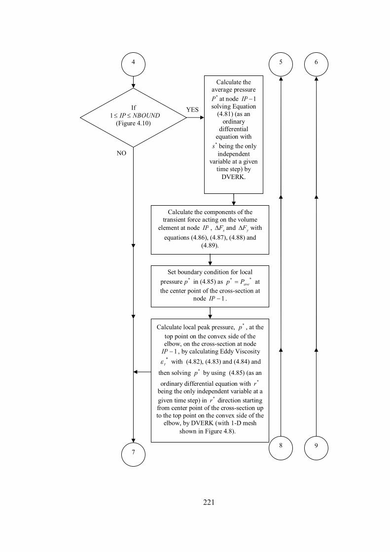
221

If NBOUNDIP 1

(Figure 4.10)

4 5 6

Calculate the average pressure

*P at node 1IP solving Equation

(4.81) (as an ordinary

differential equation with *s being the only independent

variable at a given time step) by

DVERK.

Calculate the components of the transient force acting on the volume

element at node IP , xF and yF with equations (4.86), (4.87), (4.88) and

(4.89).

Calculate local peak pressure, *p , at the top point on the convex side of the elbow, on the cross-section at node

1IP , by calculating Eddy Viscosity *

t with (4.82), (4.83) and (4.84) and

then solving *p by using (4.85) (as an

ordinary differential equation with *r being the only independent variable at a given time step) in *r direction starting from center point of the cross-section up to the top point on the convex side of the

elbow, by DVERK (with 1-D mesh shown in Figure 4.8).

Set boundary condition for local pressure *p in (4.85) as *

ave* Pp at

the center point of the cross-section at node 1IP .

7

YES

NO

8

9

222

If 1 NSTOTIPNBOUND

(Figure 4.10)

7 8

9

Calculate y component of the transient force, yF ,

acting on the volume element at node IP , with equations (4.86), (4.87)

and (4.92). ( xF =0 at node IP )

Calculate the average pressure *P at node

1IP solving Equation (4.90) (as an ordinary

differential equation with *s being the only

independent variable at a given time step) by

DVERK.

YES

NO

Set the value for the pressure at the entrance section of the elbow, *

EP , which retards to motion of the slug in the horizontal part of the pipeline, by

equating **E PP there.

Set n*n* tt 1

Store n*su

10

11

12

223

11

12 10

Write the results at node IP to the screen.

If 1IP

1 IPIP

YES

NO

If the slug upstream face has reached the entrance section

of the elbow (i.e. 050.L m.) or driving or

retarding forces acting on the slug are very close to each

other.

Write results to the screen, and output data file for the current time step.

NO

YES

Stop.

Go to the next time step

Calculate the components of the total transient force xF and yF acting on the elbow and the vertical extension

part from (4.93) and (4.94).

224

C.3 Computer Code KAYHAN in FORTRAN Language C KAYHAN.F CCCCCCCCCCCCCCCCCCCCCCCC PROGRAM DESCRIPTION CCCCCCCCCCCCCCCCC C C C This program simulates the experimental model used to C investigate the hydro-dynamics of a liquid slug motion. The C experimental model consists of an air tank and water storage tank C at the upstream. Attached to the air tank is a 31 ft long, 2" C diameter, transparent, horizontal pipe. At the downstream section of C an elbow is attached to the piping, a dynamic pressure transducer C located on this elbow is used to measure the pressures during C the impact of the liquid slug on the elbow. A certain length of a liquid C slug is generated at the upstream section by filling a segment of C the pipe by gravity through a hose connected to the water storage tank. C The U/S end of the segment now filled with water can be pressurized C by simply pressurizing the air tank to which the segment is connected. C The only mechanism keeping the liquid slug in place is a quick opening C ball valve located at the D/S end of the segment. The motion is started C by quickly opening this ball valve. The liquid slug then moves into C the initially empty pipe. During the impact around the elbow, the dynamic C pressure is recorded. C C It is the objective of this program to simulate numerically the above C described phenomenon with an acceptable accuracy by taking into C account the gas dynamics behind the slug. The program employes the C method of characterictics for the gas dynamics using the U/S air tank as C the upstream boundary and treating the slug hydro-dynamics as the moving C downstream boundary condition. The static pressure variation in the C U/S air tank is measured initially by a differential pace tranducer, C this data will be put in the program as part of the U/S boundary C conditions. The theory behind the program assumes that the ideal gas law C holds in the system. Isothermal gas law is assumed during the entire C motion. The fact that slug loses some mass during its motion in the C pipe due to frictional effects, is considred by using a coefficient C called void ratio coeff. in the slug hydro-dynamics equations. C C The program will compute air velocity, air pressure, air density C slug velocity, slug length, slug positon, and time at which those C variables are computed. C C At the time slug impacts the elbow, the peak pressure caused by the C momontum change will be computed from the velocity, density of the C slug. (i.e. (Rho)*u**2) C C Written by Zafer Bozkus, in May-June 1990. CCCCCCCCCCCCCCCCCCCCCCCCCCCCCCCCCCCCCCCCCCCCCCCCCCCCCCCCCCCCCCCCCC C C THE PRESSURE DISTRIBUTION CALCULATIONS AT THE ELBOW ARE MADE AS AN C INITIAL VALUE PROBLEM USING THE IMSL LIBRARY SUBROUTINE WITH THE C NAME Dverk, IT IS A DIFFERENTIAL EQUATION SOLVER - RUNGE KUTTA - C VERNER FIFTH AND SIXTH ORDER METHOD. C HERE IS HOW TO COMPILE THE SOURCE FILE FOR THIS PROGRAM ON VAX/VMS C USING THE OLD VERSION OF THE IMSL LIBRARY. C C FOR FILENAME (NO EXTENSION!) C LINK FILENAME, LOCAL:[IMSL.V92]IMSL/LIB (NO EXTENSION!) C RUN FILENAME (NO EXTENSION!) C C LAST MODIFIED ON April 5, 1990 (CORRECTED MOMENTUM EQUATION) C LAST MODIFIED ON JUNE 26, 1990 (ELBOW MODELING ADDDED) C (NO HOLDUP AT THE ELBOW CONSIDERED) C C----------------------------------------------------------------------- C ON November 15, 2007 A NUMERICAL ANASYSIS PART WAS ADDED FOR THE C DETERMINATION OF THE PRESSURE DISTRIBUTION AT THE ELBOW AND AT THE C EXTENSION PART DOWNSTREAM THE ELBOW, BY BÜLENT ABBAS KAYHAN. C----------------------------------------------------------------------- C ON May 24, 2008 PRESSURE DISTRIBUTION CALCULATIONS AT THE ELBOW C AND THE VRTICAL EXTENSION PART WERE DEVELOPED BY USING A C CYLINDRICAL COORDINATE SYSTEM FOR THE ELBOW PART, 2-D GAUSS C QUADRATURE FOR NUMERICAL INTEGRATION, AND A CORRELATION FUNCTION C FOR THE HOLD UP COEFFICIENT, BY BÜLENT ABBAS KAYHAN.

225

C----------------------------------------------------------------------- C PART OF THE DRIVER PROGRAM WRITTEN BY ZAFER BOZKUS ON September C 18, 1989; WAS INSERTED IN THIS CODE BY BÜLENT ABBAS KAYHAN ON July C 14, 2008 FOR THE ELBOW PART CALCULATIONS. C----------------------------------------------------------------------- C DeltaFy AND DeltaFy VALUES AT THE ELBOW AND THE VERTICAL C EXTENSION PART ALONG THE S-CURVE WERE CALCULATED BY MAKING A C CONTROL VOLUME ANALYSIS AND ADDED TO THE CODE ON October 15, 2008. C----------------------------------------------------------------------- C A CRITERIA WAS INCORPORATED TO THE CODE TO STOP THE CALCULATIONS C JUST BEFORE UNSTABLE OSCILLATIONS START TO APPEAR DURING THE C SIMULATION, ON November 15, 2008 C----------------------------------------------------------------------- CCCCCCCCCCCCCCCCCCCCCCC VARIABLE IDENDIFICATION CCCCCCCCCCCCCCC C C C V Gas velocity, m/sec. AND/OR Slug velocity, m/sec. C P Gas pressure, Pa abs. C LSS Slug length, m. C X Slug position, m. C PLL Pipe length, m. C T Time , sec. C DT Time increment used in the U/S boundary computations, sec. C DT1 Time increment used in the D/S boundary computations, sec. C DT2 Time increment used in the D/S boundary computations, sec. C DA Density of gas (air), kg/m3 C DW Density of liquid (water), kg/m3 C VF Void fraction coefficient, 0 < AL <1.0 C C Speed of gas presssure wave, m/sec. C FA Friction factor for gas (air). C FW Friction factor for liquid (water). C FDA A constant used in the equations, defined in the program C FDW A constant used in the equations, defined in the program C RTO A constant used in the equations, defined in the program C PP A constant defined in the program C EP Elbow Location= Pipe length +Initial Slug Length C A, B Abbreviated expressions used in the equations, defined in C the program C S, L and R, Subscripts for initial, U/S and D/S conditions respect. C CCCCCCCCCCCCCCCCCCCCCCCCC PROCESS BLOCK CCCCCCCCCCCCCCCCCCCCCCCCCC C PARAMETER(N1=10010,N3=10010,N4=2000) IMPLICIT REAL*8 (A-H,O-Z) REAL*8 LR,LS,LSS,EP,LSTAR,LO,LOO,SPPE,PPE,SAT,ELLOC REAL*8 MUA,MUW REAL*8 MOM(N1),LOC(N1) CHARACTER*15 FINP,FDAT,FOUT,FDAT2,FDAT3,FPLOT,FDIM,ANSW,ANS,ANS2 DIMENSION PL(N1),VL(0:N1),TL(N1),DAL(N1),DAS(0:N1),TS(0:N1), *VS(0:N1),PT(N1) DIMENSION PS(0:N1),XS(0:N1),LS(0:N1),PR(N1),VR(N1),XR(N1),LR(N1), *T(N1) DIMENSION TR(N1),XL(N1) REAL*8 DRCLST(N4) REAL*8 PP INTEGER N,IND,NW,IER,K,L,N2 INTEGER NELBW,NUM,MR,MC,ML,MLD,MSHSZ,NEXTSN,NSTOT,IP,NLBF,NLFF,NB INTEGER NSLUG INTEGER MLPRSS REAL*8 Y(1:3),C(24),W(3,9),X,TOL,XEND,SST,TM REAL*8 C1,C2,C3,F,D,PB,A,RO,TI,TIIN,MP(N1),IMPULSE REAL*8 R0,R,KM,G,MU,TCD,TFD,PI,TC,TF,MRT,UAVE,Q,QST REAL*8 LELBW,LEXTSN,LSLIMP,LTOT,ACRSS,PWET,TPR,LPR,UPR,UM,UMST REAL*8 UM1ST,UM2ST,RM1ST,RM2ST,TC1,TC2 REAL*8 RM,RMST,DKSI,DKSIST,DETA,EMELRT,DSC,DSLAST,DSCST,DSCLST REAL*8 DBELST,DSLAS1,DSLST1 REAL*8 TCDMAX,TCLMAX REAL*8 TCMAX,SCMAX,SCELB,BS,BSL,BSU,AS,HS REAL*8 DBETA,SCST,SCEDST,UAVEST,DTUAST,MOMFL1,MOMFL2 REAL*8 C4,C6,C7,C8 REAL*8 C9,C10,C11,C12 REAL*8 DRDIST REAL*8 BETA REAL*8 UST,DBUST,TRARLN,UP2ST

226

REAL*8 PAVE(1),PCNVX(1),PAVEST(1),PCVXST(1) REAL*8 QPRETS,QPTSST REAL*8 EPSLN,UAVEI REAL*8 TI1,PAVE1 REAL*8 SAV,SALR,SAPR,SAPT,SAPRG,SAPTG REAL*8 XOUT(N3), Y1OUT(0:N3), Y2OUT(N3), SSOUT(N3), PDOUT(N3,N4) REAL*8 DFXOUT(N3,N4),DFYOUT(N3,N4) REAL*8 FXOUT(N4),FYOUT(N4) REAL*8 CLSTRT REAL*8 DSCST1,DBETA1 REAL*8 PAVNST,PAVUST,PAVMST,PAVDST,PAVPST REAL*8 SCNST,SCUST,SCMST,SCDST,SCPST REAL*8 FXST,FYST,FX,FY REAL*8 SCSTCP REAL*8 SNMST,PNMST,PNM1ST,PNM2ST,PPEAST COMMON/ COEFFS/ C1, C2, C3 COMMON/ CONST/PB,RO,PAVE,MU CHARACTER CC*15 EXTERNAL UST,DBUST,TRARLN,UP2ST,PDS1ST,PDS2ST,PCTFST COMMON /PRMTS1/ R,TC,TF,QST,PI COMMON /PRMTS2/ RMST,UMST,LPR,UPR,TPR COMMON /PRMTS3/ DKSIST,DETA COMMON /PRMTS4/ R0,DBETA,DSCST COMMON /PRMTS5/ MR,MC,ML COMMON /PRMTS6/ EMELRT COMMON /PRMTS7/ TCMAX,SCMAX,SCELB COMMON /PRMTS8/ BSL,BSU,NB COMMON /PRMTS13/ QPTSST,TIST COMMON /PRMTS14/ EPSLN,D,F COMMON /PRMTS15/ DRCLST COMMON /PRMTS16/ DSCST1,DBETA1 COMMON /PRMTS17/ UM1ST,UM2ST,RM1ST,RM2ST,TC1,TC2 COMMON /PRMTS18/ PAVUST,PAVDST COMMON /PRMTS19/ SCUST,SCMST,SCDST COMMON /PRMTS20/ ACRSS COMMON /PRMTS21/ SCSTCP COMMON /TERMS2/ C4,C6,C7,C8 COMMON /TERMS3/ C9,C10,C11,C12 COMMON /TERMS4/ DRDIST,MLD COMMON /TERMS6/ BETA,G COMMON /W/ C15 COMMON /DBDVR/ IP,IPD EXTERNAL FCN2 C----- C C ------------------------ ENTER INPUT DATA ------------------------ C C----- WRITE(*,33) 33 FORMAT (' PLEASE ENTER NAME OF INPUT FILE:',$) READ(5,'(A)') FINP OPEN(UNIT=1,FILE=FINP,FORM='FORMATTED',STATUS='OLD') READ(1,271) N 271 FORMAT(//,I10) WRITE(*,66) 66 FORMAT(' ENTER NAME OF TANK PRESSURE DATA FILE:',$) READ(*,'(A)') FDAT OPEN(UNIT=3,FILE=FDAT,FORM='FORMATTED',STATUS='OLD') DO 6 M=1, N READ(3,*) T(M) , PL(M) 6 CONTINUE PRES=PL(1) PRI=PRES WRITE(*,67) 67 FORMAT(' ENTER THE NAME OF THE PEAK PRESSURE TIME HISTORY OUTPUT D *ATA FILE:',$) READ(*,'(A)') FDAT2 OPEN(UNIT=7,FILE=FDAT2,FORM='FORMATTED',STATUS='NEW') WRITE(*,68) 68 FORMAT(' ENTER THE NAME OF THE TIME HISTORIES OUTPUT DATA FILE FOR * Fx AND Fy:',$) READ(*,'(A)') FDAT3 OPEN(UNIT=8,FILE=FDAT3,FORM='FORMATTED',STATUS='NEW') C-----------------------------------------------------------

227

READ(1,273) EPSLN,D READ(1,273) DA,DW READ(1,273) MUA,MUW READ(1,274) PLL READ(1,274) TEMP READ(1,274) PO READ(1,273) VF,XI READ(1,274) LSS READ(1,274) R0 READ(1,274) G READ(1,274) LEXTSN READ(1,274) KM READ(1,274) PAVE(1) READ(1,275) MR READ(1,274) MRT READ(1,275) ML READ(1,274) CLSTRT READ(1,275) MLPRSS READ(1,275) NSLUG READ(1,274) SCMAX 272 FORMAT(/,F16.7,F16.7,F16.7) 273 FORMAT(/,F16.7,F16.7) 274 FORMAT(/,F16.7) 275 FORMAT(/,I10) CLOSE(UNIT=1) WRITE(*,35) EPSLN,D,DA,DW,MUA,MUW,PLL,TEMP,PO,VF,XI,LSS,PRES,N WRITE(*,36) R0,G,LEXTSN,KM,PAVE(1),MR,MRT,ML,NSLUG,SCMAX 35 FORMAT(/,4X,' EPSLN=',F12.8,2X,' D=',F7.4,2X,' DA=',F8.2,2X,' DW=' +,F8.2,/,4X,' MUA=',F10.8,2X,' MUW=',F10.8,2X,' PLL=',F7.3,2X, +' TEMP=',F5.1,/,4X,' PO=',F10.1,2X,' VF=',F7.4,2X,' XI=',F6.2,2X, +' LSS=',F7.3,/,4X,' PRES=',F10.4,2X,' N=',I7/) 36 FORMAT(4X,' R0=',F7.4,2X,' G=',F6.4,2X,' LEXTSN=',F8.4,2X,' KM=', +F6.2,2X,/,4X,' Boundary value for PAVE(1)=',F14.4,/,4X,' MR=',I6, +2X,' MRT=',F6.2,2X,' ML=',I6,2X,' NSLUG=',I5,2X,' SCMAX=',F7.3) C------------------------------------------------------------- WRITE(*,98) 98 FORMAT(' PLEASE ENTER NAME FOR SCREEN OUTPUT DATA FILE:',$) READ(*,'(A)') FPLOT OPEN(UNIT=2,FILE=FPLOT,FORM='FORMATTED',STATUS='NEW') C-------------------- WRITE(2,35) EPSLN,D,DA,DW,MUA,MUW,PLL,TEMP,PO,VF,XI,LSS,PRES,N WRITE(2,36) R0,G,LEXTSN,KM,PAVE(1),MR,MRT,ML,NSLUG,SCMAX C-------------------- WRITE(*,93) 93 FORMAT(' WOULD YOU LIKE TO CREATE A DIMENSIONLESS PARAMETER FILE F +OR THE HORIZONTAL',/,' PART OF THE PIPE LINE ? TYPE (Y) ES OR (N) +O:',$) READ(*,'(A)') ANSW C------------------------------------------------------------- IF(ANSW(1:1).EQ.'Y'.OR.ANSW(1:1).EQ.'y') THEN SAYI=1. WRITE(*,94) 94 FORMAT (' Enter Name for Dimensionless Output File:',$) READ(*,'(A)') FDIM OPEN(UNIT=4,FILE=FDIM,FORM='FORMATTED',STATUS='NEW') ENDIF C----------------------------------------------------------- C---------------------------------- DO 7 I = 1, N C converting the U/S gage pressure in psi to abs. pressure in pascals) PL(I) = ((PL(I)/14.7) + 1.)*PO !Equation (3) U/S C setting the U/S boundary position equal to zero. XL(I) = 0. 7 CONTINUE C---------------------------------- C--------COMPUTATION COEFFICIENTS----------------------------- C------------------------------------------------------------- TABS=TEMP+273 CWS = SQRT(287.0*TABS) !Equation (5) C---------------- PP = 2*PLL + XI !computation of stopping criterion value EP = PLL+ LSS !computation of slug location ELLOC=EP C----------------

228

WRITE(*,34) TABS,CWS,PP,EP WRITE(2,34) TABS,CWS,PP,EP 34 FORMAT(/,4X,' TABS=',F7.2,2X,' CWS=',F11.5,2X,' PP=',F9.4,2X, *'EP=',F9.4,/) C----- C----- C------------------------------------------------------------- C------------BOUNDARY CONDITIONS------------------------------ C-- The initial conditions or known values at the earlier time C-- steps have the subscript, S. C-- The unkowns at U/S boundary have the subscript, L. C-- The unkowns at D/S boundary have the subscript, R. C------------------------------------------------------------- C 999 IF (PLL/LSS.LE.6.6519) THEN VF1=0.0385*(PLL/LSS)+0.7439 ELSE VF1=1. ENDIF C ABOVE EQUATION IS A CORRELATION FUNCTION USED FOR VOID COEFICIENT C CALCULATION RTO=2*(1-VF1)/VF1 AA = 0.5*RTO C---------------------------------------------------------- C setting the initial conditions XS(0) = XI LS(0) = LSS VS(0) = 0. TS(0) = 0. PS(0) = PL(1) ALPHA = 0. DT1 = 0. DAS(0)=PL(1)/CWS**2 COUNT=0. C--------------------------------------------------------------------- C C----------------------------------------------------------------------- WRITE(*,108) WRITE(2,108) 108 FORMAT(//,1X,'TR(sec.)',1X,'PR(psi)',1X,'VR(m/s)',1X,'LR(m)',2X, +'LOC(m)',1X,'MOM(psi)',1X,'TL(sec)',1X,'PL(psi)',1X,'VL(m/s)', +1X,'dP/dx') C------------------------------------------------------------------- IF (SAYI.EQ.1.0) THEN WRITE(4,777) 777 FORMAT(' TSTAR PSTAR LSTAR XSTAR VSTAR') ENDIF C------------------------------------------------------------------- C VL(0)=0. C------------- ACTUAL COMPUTATIONS --------------------------------- DO 20 I=0,N J=I+1 K=J+1 C IF (PLL/LS(I).LE.6.6519) THEN VF=0.0385*(PLL/LS(I))+0.7439 ELSE VF=1. ENDIF RTO=2*(1-VF)/VF C------------------------------------------------------------------- IF (VL(J-1).NE.0.) THEN CALL FCAL(ABS(VL(J-1)),DA,MUA,EPSLN,D,FA) ELSE FA=0. ENDIF FDA = FA/(2*D) C------------------------------------------------------------------- C ABOVE EQUATION IS A CORRELATION FUNCTION USED FOR VOID COEFICIENT C CALCULATION C---------UPSTREAM BOUNDARY COMPUTATIONS---------------------------- C TL(J) = TS(I) + (XL(J)-XS(I))/(VS(I)-CWS) !Equation (2) U/S

229

DT = TL(J) - TS(I) !Equation (6) U/S C----- ALPHA = TL(J) CALL LINEAR(T,PL,N,ALPHA,S) PT(J)=S C PL(J) = S DAL(J) = S/CWS**2 !Equation (4) U/S C----- R= (CWS*DAS(I)*(FDA*VS(I)*DT+1.0)) VL(J)=(S-PS(I)+CWS*DAS(I)*VS(I))/R !Equation (1) U/S C C--------- DOWNSTREAM BOUNDARY COMPUTATIONS------------------------- C C------------------------------------------------------------------- IF (VS(I).NE.0.) THEN CALL FCAL(VS(I),DA,MUA,EPSLN,D,FA) ELSE FA=0. ENDIF IF (VS(I).NE.0.) THEN CALL FCAL(VS(I),DW,MUW,EPSLN,D,FW) ELSE FW=0. ENDIF FDW = FW/(2*D) FDA = FA/(2*D) C------------------------------------------------------------------- C..........Following Equation is equation (8) D/S.................... XR(K) =((VS(I)*DT+XS(I))*(VL(J)+CWS)-XL(J)*VS(I))/((VL(J)+ *CWS)-VS(I)) DT1 = (XR(K) - XL(J))/(VL(J)+CWS) !Equation (2) D/S TR(K) = TL(J) + DT1 !Equation (2) D/S DT2 = TR(K) - TS(I) !Equation (4) D/S LR(K) = LS(I)-0.5*RTO*VS(I)*DT2 !Equation (5) D/S A = (FDA*VL(J)*DT1 + 1)*DAL(J)*CWS B = 1+(FDW - RTO/LS(I))*VS(I)*DT2 PR(K) = S+DAL(J)*CWS*VL(J) - 2(A/B)*((1./DW)*((PS(I)-PO)/LS(I))*DT2 + VS(I)) !Equation (1) D/S VR(K) = ((1./DW)*((PS(I)-PO)/LS(I))*DT2 + VS(I))/B !Equation (6) D/S C--------------PRINTING DATA FOR PLOTS--------------------------------------- MOM(K)=(DW*VR(K)**2)/6891.1565 !RHO*V**2 Term in psi. LOC(K)=XR(K)+LR(K)-XI !Front Loc. from U/S elbow C--------------------------------------------------------------------------- C--- Computation of slug arrival time and paek pressure at the elbow, using C--- interpolation. IF(COUNT.EQ.0.AND.LOC(K).GE.EP) THEN SAT = TR(K-1) + ((TR(K)-TR(K-1))*(EP-LOC(K-1)))/(LOC(K)-LOC(K-1)) SAV = VR(K-1) + ((VR(K)-VR(K-1))*(EP-LOC(K-1)))/(LOC(K)-LOC(K-1)) PPE = MOM(K-1)+((MOM(K)-MOM(K-1))*(EP-LOC(K-1)))/(LOC(K)-LOC(K-1)) SALR = LR(K-1) + ((LR(K)-LR(K-1))*(EP-LOC(K-1)))/(LOC(K)-LOC(K-1)) SAPR = PR(K-1) + ((PR(K)-PR(K-1))*(EP-LOC(K-1)))/(LOC(K)-LOC(K-1)) SAPT = PT(J-1) + ((PT(J)-PT(J-1))*(EP-LOC(K-1)))/(LOC(K)-LOC(K-1)) COUNT=1 ENDIF C--------------------------------------------------------------------------- PSK=(PR(K)-PO)/6891.1565 !Gage press. behind slug PSJ=(S-PO)/6891.1565 !Gage press.in the tank C--------- PX=(PSJ-PSK)/TR(K) C--------- WRITE(*,109)TR(K),PSK,VR(K),LR(K),LOC(K),MOM(K),TL(J),PSJ,VL(J),PX WRITE(2,109)TR(K),PSK,VR(K),LR(K),LOC(K),MOM(K),TL(J),PSJ,VL(J),PX 109 FORMAT(1X,F7.5,2X,F6.3,1X,F7.3,1X,F6.4,1X,F6.3,1X,F7.2,2X, 2F8.6,2X,F6.3,1X,F6.3,1X,F7.5) C------ C------------------------------------------------------------------- C---- COMPUTE THE SCALED PARAMETERS TO BE USED LATER. IF (I.EQ.0) THEN CALL FCAL(VR(K),DW,MUW,EPSLN,D,FW) LO= (2*D/FW)*(1-AA) !Length Scaling Parameter VO = SQRT((PRES*6891.1565)/DW) !Velocity Scaling Parameter TO = LO/VO !Time Scaling Parameter ENDIF C------COMPUTE AND PRINT DIMENSIONLESS PARAMETERS

230

C------ IF(SAYI.EQ.1.0) THEN VSTAR = VR(K)/VO !Scaled Slug Velocity PSTAR = PSK/PRES !Scaled Driving Pressure LSTAR = LR(K)/LO !Scaled Slug Length TSTAR = TR(K)/TO !Scaled Time XSTAR = LOC(K)/LO !Scaled Slug Position WRITE(4,110) TSTAR, PSTAR, LSTAR, XSTAR, VSTAR 110 FORMAT(F10.6,2X,F10.7,2X,F10.7,2X,F10.5,2X,F10.5) ENDIF C------------------------------------------------------------------- C--------------------------- C STOPPING CRITERIA C WHEN INPUT DATA TIME RANGE WAS PASSED/OR THE SLUG PASSED THE C ELBOW BY PLL AND/OR SLUG LENGTH REDUCES TO ZERO. IF(TR(K).GT.(0.98*T(N)).OR.XR(K).GE.PP.OR.LR(K).LE.0.10) THEN 888 WRITE(*,106) C WRITE(3,106) 106 FORMAT( ' SLUG LENGTH HAS APPROACHED ZERO!',/, + ' OR SLUG TRAVELLED THE SPECIFIED DISTANCE!',/, + ' OR INPUT DATA TIME RANGE WAS PASSED!!!') WRITE(*,111)SAT,PPE,EP WRITE(2,111)SAT,PPE,EP 111 FORMAT( ' Slug arrived at the elbow at ',1X,F7.5,1X,'sec.',/, + ' peak pressure due to momentum was ',F8.2,1X,'psig',/, + ' Elbow location is ',1X,F6.3,1X,'meters',///) GO TO 200 ELSE CONTINUE ENDIF C C SLUG Subscript Adjustments TS(I+1) = TR(K) VS(I+1) = VR(K) PS(I+1) = PR(K) XS(I+1) = XR(K) LS(I+1) = LR(K) DAS(I+1) =PR(K)/CWS**2 C 20 CONTINUE C C---Compute scaled arrival time, peak pressure,and elbow location C C------------------------------- 200 IF(SAYI.EQ.1.0) THEN SAT=SAT/TO PPE = PPE/PRES EP = EP/LO WRITE(4,112)SAT,PPE,EP WRITE(4,113)TO,VO,LO,PRES WRITE(*,112)SAT,PPE,EP WRITE(*,113)TO,VO,LO,PRES ENDIF C----------------------------------------------------------------------- 112 FORMAT( //' Scaled Arr. Time at the elbow is ',1X,F9.5,/, + ' Scaled Peak Pres. at the elbow is ',F8.4,/, + ' Scaled Elbow Location is ',1X,F6.3,//) C----------------------------------------------------------------------- 113 FORMAT( ' Scaling parameter for time was T =',2x,F7.5,1x,'sec.',/, + ' Scaling parameter for vel. was V =',2x,F10.2,1x,'m/s',/, + ' Scaling parameter for length was L =',2x,F10.7,1x,'m',/, + ' Scaling parameter for pressure was Pi=', F7.3,1x,'psig') C----------------------------------------------------------------------- Y1OUT(0)=SAV C--------------------------------------------------------- C----------------CALCULATIONS FOR THE ELBOW--------------- C--------------------------------------------------------- N2=N 199 CONTINUE WRITE(*,202) 202 FORMAT(1X,'Initializations for the arrays are being made...') DO 201 II=1,N3 DO 201 JI=1,N4 PDOUT(II,JI)=0.

231

DFXOUT(II,JI)=0. DFYOUT(II,JI)=0. 201 CONTINUE WRITE(*,203) 203 FORMAT(1X,'Initializations for the arrays were completed.',///) DO 198 I = 1, N2 C converting th U/S abs. pressure in pascals to gage pressure in pascals PL(I) = PL(I)-PO 198 CONTINUE MU=MUW RO=DW PI=4.*ATAN(1.) R=D/2. QPRETS=Y1OUT(0)*PI*R**2 PWET=2*PI*R ACRSS=PI*R**2 LELBW=1/4.*2*PI*R0 C Derived Lengths LSLIMP=SALR DSC=LSLIMP/NSLUG TIIN=DSC/SAV WRITE(*,232) 'Space increment along the s-curve, DSC (m.) :',DSC WRITE(2,232) 'Space increment along the s-curve, DSC (m.) :',DSC 232 FORMAT(1X,A45,F12.8) TPR=TIIN LPR=2*LELBW/KM UPR=LPR/TPR QPTSST=QPRETS/(UPR*LPR**2) C For the elements of the computational mesh at any cross- C section of the pipe: C MR= number of mesh elements radial direction; MC= number of mesh C elements in the circumferential direction. MC=MR*MRT MSHSZ=MR*MC WRITE(*,230) "Mesh size over the pipe cross-section: MR x MC=",MR, *" x",MC WRITE(2,230) "Mesh size over the pipe cross-section: MR x MC=",MR, *" x",MC 230 FORMAT(/,1X,A47,I5,A3,I5) DKSI=R/MR DKSIST=DKSI/LPR DETA=2*PI/MC C--------------------------------- WRITE(*,233) "Maximum mesh size for the line integrals at any cros *s-section: ML=",ML WRITE(2,233) "Maximum mesh size for the line integrals at any cros *s-section: ML=",ML 233 FORMAT(1X,A66,I5,A3,I5) C--------------------------------- C--------------------------------- C For the nodal points of the computational mesh along the C elbow: C The starting node at the upstream end of the elbow is NODE 1. EMELRT=1./100 C EMERLT: End Mesh Element Lentgth Ratio NELBW=LELBW/DSC+1 DSLAS1=LELBW-(NELBW-1)*DSC DSLST1=DSLAS1/LPR C The criteria here in this IF statement above was also used C for the starting node (NSTOT) of the backward calculational C procedure along the curve s. IF (DSLST1.LE.DSC*EMELRT) THEN NELBW=NELBW-1 DSLST1=0. ENDIF NEXTSN=LEXTSN/DSC+1 DSLAST=LEXTSN-(NEXTSN-1)*DSC C The criteria here in this IF statement above was also used C for the starting node (NSTOT) of the backward calculational C procedure along the curve s. IF (DSLAST.LE.DSC*EMELRT) THEN NEXTSN=NEXTSN-1 DSLAST=0. ENDIF

232

DSCST=DSC/LPR DSCLST=DSLAST/LPR NSTOT=NELBW+NEXTSN LTOT=LELBW+LEXTSN LTOTST=LTOT/LPR SCEXT=LTOT SCENT=0. DBETA=DSC/R0 DBELST=DSLST1/R0 NLBF=0 NLFF=0 WRITE(*,262) NELBW WRITE(2,262) NELBW 262 FORMAT(1X,'Total number of volume elements along the elbow: NELBW= *',I5) WRITE(*,261) NSTOT WRITE(2,261) NSTOT 261 FORMAT(1X,'Total number of volume elements along the total s-curve *: NSTOT=',I5) WRITE(*,270) MLPRSS WRITE(2,270) MLPRSS 270 FORMAT(1X,'Mesh size along the pipe radius for local pressure calc *ulation at the',/,1X,'pipe wall: MLPRSS=',I5,/) C Clustering of the line mesh for the line integral. CALL MCLSTR(R,ML,CLSTRT,DRCLST) C--------------------------------- C An initial calculation for the value of the friction angle TF. UAVEI=SAV IF (UAVEI.NE.0.) THEN CALL TFCAL(UAVEI) ELSE F=0. ENDIF C--------------------------------- TCLMAX=TF*180/PI TCDMAX=0.0124*(PLL/LSS)**3-0.2072*(PLL/LSS)**2+1.1001*(PLL/LSS) *+87.951 WRITE(*,269) TCDMAX WRITE(2,269) TCDMAX 269 FORMAT(1X,"Maximum calibration angle of the velocity profile in de *grees that occurs along",/," the s-curve: TCDMAX=",F9.5,/) IF (TCDMAX.GT.TCLMAX) THEN WRITE(*,281) TCLMAX WRITE(2,281) TCLMAX 281 FORMAT(1X,'The calculated maximum calibration angle TCDMAX is grea *ter than',F9.4,/,' degree, which is the maximum allowable value.') WRITE(*,282) WRITE(2,282) 282 FORMAT(/,1X,'Program failed to continue...') STOP ENDIF SCELB=LELBW TCMAX=TCDMAX/180*PI C--------------------------------- C The nodal point on the elbow axis, for which the maximum C presure at the convex side of the elbow occurs, is calculated C here. NMAXP=INT((SCMAX/LPR-DSCST/2.)/DSCST+0.5+0.5)+1 WRITE(7,13) 'NMAXP=',NMAXP 13 FORMAT(1X,A6,I5,//) WRITE(7,12) 'Time(s)','Peak Pressure(psi)' 12 FORMAT(4X,A7,12X,A18) C--------------------------------- WRITE(8,17) 'Time(s)','Fx (N)','Fy (N)' 17 FORMAT(4X,A7,8X,A6,8X,A6) C--------------------------------- WRITE(*,15) 'Output for the Pressure Distribution at each Time Ste *p:' 15 FORMAT(//,1X,A55) WRITE(2,14) 14 FORMAT(//,1x,'T (sec.)',3X,'VF (m/s)',3X,'LSS (m)' *,2X,'Tank (psi)',5X, 'Rise ',3x,'Scaled Rise'/) C--------------------------------- J=0

233

FROLST=0. XEND=SAT XPRE=XEND Y(1)=SAV Y(2)=SALR SAPRG=SAPR-PO SAPTG=SAPT-PO C---------------------------------------------------------- DO 16 I = K, N2 C--------------------------------- TI=DSC/Y(1) UAVE=Y(1) IF (UAVE.NE.0.) THEN CALL TFCAL(UAVE) ELSE F=0. ENDIF FXST=0. FYST=0. C1 = (F/(2*D)) C--------------------------------- C SET INITIAL FLAGS C--------------------------------- NW = 3 N = 2 X =XEND TOL = 0.0001 IND=1 XEND = XEND+TI C------------------------------- J=J+1 ALPHA=XEND CALL LINEAR(T,PL,N2,ALPHA,S) PB=S-(SAPTG-SAPRG) C Above substruction for tank pressure was made for the head loss C along the part of the pipeline filled with air. PB here is the C driving gage presure applied by the air at the upstream side of C the slug. SS = PB/6891.1565 C-------------------------------- CALL DVERK(N,FCN2,X,Y,XEND,TOL,IND,C,NW,W) MP(I) = RO*Y(1)**2 PSI = MP(I)/6891.1565 PPE = PSI/PRI C-------------------------------- XOUT(J)=X Y1OUT(J)=Y(1) Y2OUT(J)=Y(2) SSOUT(J)=SS WRITE(*,21) 'For T=',XOUT(J),'sec:' 21 FORMAT(1X,A6,F8.5,1X,A4) WRITE(*,22) 'VF=',Y1OUT(J),'m/s','LSS=',Y2OUT(J),'m','Driving Pr.= *',SSOUT(J),'psi' 22 FORMAT(1X,A3,F9.4,1X,A3,2X,A,F6.3,1X,A1,2X,A12,F8.4,1X,A3) WRITE(*,18) 'NODE','PRESSURE RISE (psi)','deltaFx (N)', *'deltaFy (N)' 18 FORMAT(1X,A4,3X,A19,10X,A11,6X,A11) C--------------------------------- C Parameters for the subroutine DVERK defined again NW=1 N=1 SCST=0. TOL=0.0001 IND=1 C--------------------------------------------------- UAVE=Y1OUT(J) UAVEST=UAVE/UPR Q=UAVE*PI*R**2 QST=Q/(UPR*LPR**2) TIST=TI/TPR C------------------------------------------------------------------ C Calculating the boundary values at the exit of the vertical C extension part. PAVE(1)=0.

234

PAVEST(1)=PAVE(1)/(RO*UPR**2) PAVMST=0. C------------------------------------------------------------------ FROLST=FROLST+UAVEST*TIST IF (FROLST.LT.DSCST/2.) THEN NLFF=0 ELSE IF (FROLST.GE.DSCST/2. .AND.FROLST.LE.LELBW/LPR+DSCST/2. *.AND.DBELST.LE.EMELRT*DBETA) THEN NLFF=1+INT((FROLST-DSCST/2.)/DSCST) ELSE IF (FROLST.GE.DSCST/2. .AND.FROLST.LT.LELBW/LPR-DSLST1. *AND.DBELST.GT.EMELRT*DBETA) THEN NLFF=1+INT(FROLST/DSCST) ELSE IF (FROLST.GE.LELBW/LPR-DSLST1.AND.FROLST.LT.LELBW/LPR- *DSLST1/2. .AND.DBELST.GT.EMELRT*DBETA) THEN NLFF=1+INT((FROLST-DSLST1/2.)/DSCST) ELSEIF (FROLST.GE.LELBW/LPR-DSLST1/2. AND.FROLST.LT.LELBW/ *LPR .AND. DBELST.GT.EMELRT*DBETA) THEN NLFF=NELBW ELSE IF (FROLST.GE.LELBW/LPR.AND.FROLST.LT.LTOT/LPR-DSCST/2. *.AND.DSCLST.LT.DSCST*EMELRT) THEN NLFF=NELBW+INT((FROLST-LELBW/LPR)/DSCST) ELSE IF (FROLST.GE.LELBW/LPR.AND.FROLST.LT.LTOT/LPR-DSCLST/2. *.AND.DSCLST.GT.DSCST*EMELRT) THEN NLFF=NELBW+INT((FROLST-LELBW/LPR)/DSCST) ELSE IF (FROLST.GE.LTOT/LPR-DSCST/2. .AND.FROLST.LT.LTOT/LPR *.AND.DBELST.LT.EMELRT*DBETA) THEN NLFF=NSTOT ELSE IF (FROLST.GE.LTOT/LPR-DSCLST/2. .AND.FROLST.LT.LTOT/LPR *.AND.DBELST.GT.EMELRT*DBETA) THEN NLFF=NSTOT ELSE IF (FROLST.GE.LTOT/LPR) THEN NLFF=NSTOT+1 ENDIF DTUAST=(Y1OUT(J)/UPR-Y1OUT(J-1)/UPR)/TIST C4=-DTUAST C9=C4 C Calculations for average pressure are being made by using C backward differences at point IP-1 (at coordinate SCEND on C curve s). C Calculations for deltaFx and deltaFy are being made at point C IP using control volume approach. DO 220 IP=NLFF,NLBF+1,-1 IND=1 IF (IP.LE.NELBW) THEN C---------------- IF ((IP.LT.NELBW.OR.DBELST.LE.EMELRT*DBETA).AND.IP.EQ.NLBF+1) THEN SCST=(IP-1)*DSCST+DSCST/2. SCEDST=(IP-1)*DSCST DSCST1=DSCST/2. DBETA1=DSCST1*LPR/R0 CALL UMSTCL(SCST) IF (IP.EQ.NLFF) CALL INCRAR(SCST,UP2ST,MOMFL2) CALL UMSTCL(SCEDST) CALL INCRAR(SCEDST,UP2ST,MOMFL1) C6=-LPR**3/(R0*ACRSS)*(MOMFL2-MOMFL1)/DBETA1 C7=-LPR*(F*PWET/(8*ACRSS))*UAVEST**2-UAVEST**2 BETA=DBETA*(IP-1)+DBETA/2. C8=LPR*G/UPR**2*SIN(BETA) C SCEND MUST BE SMALLER THAN SC BECAUSE THE COMPUTATION C IS BEING MADE BACKWARDS HERE, ALONG THE 1-D MESH, WITH C SUBROUTINE DVERK. CALL DVERK(N,PDS1ST,SCST,PAVEST,SCEDST,TOL,IND,C,NW,W) IF (IP.LE.NSTOT.AND.IP.LT.NLFF) THEN SCUST=(IP-1)*DSCST SCMST=(IP-1)*DSCST+DSCST/2. SCDST=(IP-1)*DSCST+DSCST SCPST=(IP-1)*DSCST+DSCST+DSCST/2. PAVUST=PAVEST(1) CALL PINTER(PAVDST,SCDST,PAVMST,PAVPST,SCMST,SCPST) CALL DFELBW(DFXST,DFYST) ENDIF C---------------- ELSE IF (IP.LT.NELBW) THEN SCST=(IP-1)*DSCST+DSCST/2.

235

SCEDST=(IP-2)*DSCST+DSCST/2. DSCST1=DSCST DBETA1=DSCST1*LPR/R0 CALL UMSTCL(SCST) IF (IP.EQ.NLFF) CALL INCRAR(SCST,UP2ST,MOMFL2) CALL UMSTCL(SCEDST) CALL INCRAR(SCEDST,UP2ST,MOMFL1) C6=-LPR**3/(R0*ACRSS)*(MOMFL2-MOMFL1)/DBETA1 C7=-LPR*(F*PWET/(8*ACRSS))*UAVEST**2-UAVEST**2 BETA=DBETA*(IP-1)+DBETA/2. C8=LPR*G/UPR**2*SIN(BETA) CALL DVERK(N,PDS1ST,SCST,PAVEST,SCEDST,TOL,IND,C,NW,W) IF (IP.LE.NSTOT.AND.IP.LT.NLFF) THEN SCNST=(IP-2)*DSCST+DSCST/2. SCUST=(IP-2)*DSCST+DSCST/2.+DSCST/2. SCMST=(IP-1)*DSCST+DSCST/2. SCDST=(IP-1)*DSCST+DSCST/2.+DSCST/2. SCPST=(IP-1)*DSCST+DSCST/2.+DSCST/2.+DSCST/2. IF (IP.EQ.NELBW-1 .AND.DBELST.GT.EMELRT*DBETA) SCPST=(IP-1)*DSCST+ *DSCST/2.+DSCST/2.+DSLST1/2. PAVNST=PAVEST(1) CALL PINTER(PAVUST,SCUST,PAVNST,PAVMST,SCNST,SCMST) CALL PINTER(PAVDST,SCDST,PAVMST,PAVPST,SCMST,SCPST) CALL DFELBW(DFXST,DFYST) ENDIF C---------------- ELSE IF (IP.EQ.NELBW.AND.DBELST.LE.EMELRT*DBETA.AND.IP.GT.1) THEN SCST=(IP-2)*DSCST+DSCST/2.+DSCST/2.+DSCST/2. SCEDST=(IP-2)*DSCST+DSCST/2. DSCST1=DSCST DBETA1=DSCST1*LPR/R0 CALL UMSTCL(SCST) IF (IP.EQ.NLFF) CALL INCRAR(SCST,UP2ST,MOMFL2) CALL UMSTCL(SCEDST) CALL INCRAR(SCEDST,UP2ST,MOMFL1) C6=-LPR**3/(R0*ACRSS)*(MOMFL2-MOMFL1)/DBETA1 C7=-LPR*(F*PWET/(8*ACRSS))*UAVEST**2-UAVEST**2 BETA=DBETA*(IP-2)+DBETA/2.+DBETA/2.+DBETA/2. C8=LPR*G/UPR**2*SIN(BETA) CALL DVERK(N,PDS1ST,SCST,PAVEST,SCEDST,TOL,IND,C,NW,W) IF (IP.LE.NSTOT.AND.IP.LT.NLFF) THEN SCNST=(IP-2)*DSCST+DSCST/2. SCUST=(IP-2)*DSCST+DSCST/2.+DSCST/2. SCMST=(IP-2)*DSCST+DSCST/2.+DSCST/2.+DSCST/2. SCDST=(IP-1)*DSCST+DSCST/2.+DSCST/2. SCPST=(IP-1)*DSCST+DSCST/2.+DSCST/2.+DSCST/2. PAVNST=PAVEST(1) CALL PINTER(PAVUST,SCUST,PAVNST,PAVMST,SCNST,SCMST) CALL PINTER(PAVDST,SCDST,PAVMST,PAVPST,SCMST,SCPST) CALL DFELBW(DFXST,DFYST) ENDIF C---------------- ELSE IF (IP.EQ.NELBW.AND.DBELST.GT.EMELRT*DBETA.AND.IP.GT.1) THEN SCST=(IP-2)*DSCST+DSCST/2.+DSCST/2.+DSLST1/2. SCEDST=(IP-2)*DSCST+DSCST/2. DSCST1=DSCST/2.+DSLST1/2. DBETA1=DSCST1*LPR/R0 CALL UMSTCL(SCST) IF (IP.EQ.NLFF) CALL INCRAR(SCST,UP2ST,MOMFL2) CALL UMSTCL(SCEDST) CALL INCRAR(SCEDST,UP2ST,MOMFL1) C6=-LPR**3/(R0*ACRSS)*(MOMFL2-MOMFL1)/DBETA1 C7=-LPR*(F*PWET/(8*ACRSS))*UAVEST**2-UAVEST**2 BETA=DBETA*(IP-2)+DBETA/2.+DBETA/2.+DBELST/2. C8=LPR*G/UPR**2*SIN(BETA) CALL DVERK(N,PDS1ST,SCST,PAVEST,SCEDST,TOL,IND,C,NW,W) IF (IP.LE.NSTOT.AND.IP.LT.NLFF) THEN SCNST=(IP-2)*DSCST+DSCST/2. SCUST=(IP-2)*DSCST+DSCST/2.+DSCST/2. SCMST=(IP-2)*DSCST+DSCST/2.+DSCST/2.+DSLST1/2. SCDST=(IP-2)*DSCST+DSCST/2.+DSCST/2.+DSLST1 SCPST=(IP-2)*DSCST+DSCST/2.+DSCST/2.+DSLST1+DSCST/2. PAVNST=PAVEST(1) CALL PINTER(PAVUST,SCUST,PAVNST,PAVMST,SCNST,SCMST)

236

CALL PINTER(PAVDST,SCDST,PAVMST,PAVPST,SCMST,SCPST) CALL DFELBW(DFXST,DFYST) ENDIF ENDIF C---------------- ELSE IF (IP.EQ.NELBW+1 .AND.DBELST.LE.EMELRT*DBETA.AND.NLFF.NE. *NELBW+1) THEN C Here, the average pressure value at the last node of the C of the elbow is calculated. C (Point NELBW+1 corresponds to the connection boundary of the C elbow and the vertical extension part as a special case here.) SCST=LELBW/LPR SCEDST=LELBW/LPR-DSCST/2. DSCST1=DSCST/2. DBETA1=DSCST1*LPR/R0 CALL UMSTCL(SCST) IF (IP.EQ.NLFF) CALL INCRAR(SCST,UP2ST,MOMFL2) CALL UMSTCL(SCEDST) CALL INCRAR(SCEDST,UP2ST,MOMFL1) C6=-LPR**3/(R0*ACRSS)*(MOMFL2-MOMFL1)/DBETA1 C7=-LPR*(F*PWET/(8*ACRSS))*UAVEST**2-UAVEST**2 BETA=DBETA*(IP-1) C8=LPR*G/UPR**2*SIN(BETA) PAVUST=PAVEST(1) CALL DVERK(N,PDS1ST,SCST,PAVEST,SCEDST,TOL,IND,C,NW,W) IF (IP.LE.NSTOT.AND.IP.LT.NLFF) THEN SCUST=LELBW/LPR SCMST=LELBW/LPR+DSCST/2. SCDST=LELBW/LPR+DSCST SCPST=LELBW/LPR+DSCST+DSCST/2. CALL PINTER(PAVDST,SCDST,PAVMST,PAVPST,SCMST,SCPST) CALL DFEXTN(DFXST,DFYST) ENDIF C---------------- ELSE IF(IP.EQ.NELBW+1 .AND.DBELST.GE.EMELRT*DBETA.AND.NLFF.NE. *NELBW+1) THEN C Here, the average pressure value at the last node of the C of the elbow is calculated. SCST=LELBW/LPR SCEDST=LELBW/LPR-DSLST1/2. DSCST1=DSLST1/2. DBETA1=DSCST1*LPR/R0 CALL UMSTCL(SCST) IF (IP.EQ.NLFF) CALL INCRAR(SCST,UP2ST,MOMFL2) CALL UMSTCL(SCEDST) CALL INCRAR(SCEDST,UP2ST,MOMFL1) C6=-LPR**3/(R0*ACRSS)*(MOMFL2-MOMFL1)/DBETA1 C7=-LPR*(F*PWET/(8*ACRSS))*UAVEST**2-UAVEST**2 BETA=DBETA*(IP-3)+DBETA/2.+DBETA/2.+DBELST C8=LPR*G/UPR**2*SIN(BETA) PAVUST=PAVEST(1) CALL DVERK(N,PDS1ST,SCST,PAVEST,SCEDST,TOL,IND,C,NW,W) IF (IP.LE.NSTOT.AND.IP.LT.NLFF) THEN SCUST=LELBW/LPR SCMST=LELBW/LPR+DSCST/2. SCDST=LELBW/LPR+DSCST SCPST=LELBW/LPR+DSCST+DSCST/2. CALL PINTER(PAVDST,SCDST,PAVMST,PAVPST,SCMST,SCPST) CALL DFEXTN(DFXST,DFYST) ENDIF C---------------- ELSE IF (IP.EQ.NELBW+1 .AND.DBELST.LE.EMELRT*DBETA.AND.NLFF.EQ. *NELBW+1) THEN SCST=LELBW/LPR+DSCST/2. SCEDST=LELBW/LPR DSCST1=DSCST/2. DBETA1=DSCST1*LPR/R0 CALL UMSTCL(SCST) IF (IP.EQ.NLFF) CALL INCRAR(SCST,UP2ST,MOMFL2) CALL UMSTCL(SCEDST) CALL INCRAR(SCEDST,UP2ST,MOMFL1) C10=-LPR**2/ACRSS*(MOMFL2-MOMFL1)/DSCST1 C11=-F*PWET/(8*ACRSS)*LPR*UAVEST**2 C12=G*LPR/UPR**2

237

CALL DVERK(N,PDS2ST,SCST,PAVEST,SCEDST,TOL,IND,C,NW,W) CONTINUE IND=1 PAV1ST=PAVEST(1) MOMFL2=MOMFL1 SCST=LELBW/LPR SCEDST=LELBW/LPR-DSCST/2. DSCST1=DSCST/2. DBETA1=DSCST1*LPR/R0 CALL UMSTCL(SCST) IF (IP.EQ.NLFF) CALL INCRAR(SCST,UP2ST,MOMFL2) CALL UMSTCL(SCEDST) CALL INCRAR(SCEDST,UP2ST,MOMFL1) C6=-LPR**3/(R0*ACRSS)*(MOMFL2-MOMFL1)/DBETA1 C7=-LPR*(F*PWET/(8*ACRSS))*UAVEST**2-UAVEST**2 BETA=DBETA*(IP-1) C8=LPR*G/UPR**2*SIN(BETA) CALL DVERK(N,PDS1ST,SCST,PAVEST,SCEDST,TOL,IND,C,NW,W) PBOUST=PAVEST(1) PAVEST(1)=PAV1ST C---------------- ELSE IF(IP.EQ.NELBW+1 .AND.DBELST.GE.EMELRT*DBETA.AND.NLFF.EQ. *NELBW+1) THEN SCST=LELBW/LPR+DSCST/2. SCEDST=LELBW/LPR DSCST1=DSCST/2. DBETA1=DSCST1*LPR/R0 CALL UMSTCL(SCST) IF (IP.EQ.NLFF) CALL INCRAR(SCST,UP2ST,MOMFL2) CALL UMSTCL(SCEDST) CALL INCRAR(SCEDST,UP2ST,MOMFL1) C10=-LPR**2/ACRSS*(MOMFL2-MOMFL1)/DSCST1 C11=-F*PWET/(8*ACRSS)*LPR*UAVEST**2 C12=G*LPR/UPR**2 CALL DVERK(N,PDS2ST,SCST,PAVEST,SCEDST,TOL,IND,C,NW,W) CONTINUE IND=1 PAV1ST=PAVEST(1) MOMFL2=MOMFL1 SCST=LELBW/LPR SCEDST=LELBW/LPR-DSLST1/2. DSCST1=DSLST1/2. DBETA1=DSCST1*LPR/R0 CALL UMSTCL(SCST) IF (IP.EQ.NLFF) CALL INCRAR(SCST,UP2ST,MOMFL2) CALL UMSTCL(SCEDST) CALL INCRAR(SCEDST,UP2ST,MOMFL1) C6=-LPR**3/(R0*ACRSS)*(MOMFL2-MOMFL1)/DBETA1 C7=-LPR*(F*PWET/(8*ACRSS))*UAVEST**2-UAVEST**2 BETA=DBETA*(IP-3)+DBETA/2.+DBETA/2.+DBELST C8=LPR*G/UPR**2*SIN(BETA) CALL DVERK(N,PDS1ST,SCST,PAVEST,SCEDST,TOL,IND,C,NW,W) PBOUST=PAVEST(1) PAVEST(1)=PAV1ST C---------------- ELSE IF (IP.GT.NELBW.AND.IP.EQ.NELBW+2) THEN SCST=LELBW/LPR+(IP-NELBW-1)*DSCST+DSCST/2. SCEDST=LELBW/LPR+(IP-NELBW-2)*DSCST+DSCST/2. DSCST1=DSCST DBETA1=DSCST1*LPR/R0 CALL UMSTCL(SCST) IF (IP.EQ.NLFF) CALL INCRAR(SCST,UP2ST,MOMFL2) CALL UMSTCL(SCEDST) CALL INCRAR(SCEDST,UP2ST,MOMFL1) C10=-LPR**2/ACRSS*(MOMFL2-MOMFL1)/DSCST1 C11=-F*PWET/(8*ACRSS)*LPR*UAVEST**2 C12=G*LPR/UPR**2 CALL DVERK(N,PDS2ST,SCST,PAVEST,SCEDST,TOL,IND,C,NW,W) IF (IP.LE.NSTOT.AND.IP.LT.NLFF) THEN SCNST=LELBW/LPR+DSCST/2. SCUST=LELBW/LPR+DSCST SCMST=LELBW/LPR+DSCST+DSCST/2. SCDST=LELBW/LPR+DSCST+DSCST SCPST=LELBW/LPR+DSCST+DSCST+DSCST/2.

238

PAVNST=PAVEST(1) CALL PINTER(PAVUST,SCUST,PAVNST,PAVMST,SCNST,SCMST) CALL PINTER(PAVDST,SCDST,PAVMST,PAVPST,SCMST,SCPST) CALL DFEXTN(DFXST,DFYST) ENDIF CONTINUE IND=1 PAV1ST=PAVEST(1) MOMFL2=MOMFL1 C Calculating the pressure value at the connection point of the C elbow and the vertical extension part. SCST=LELBW/LPR+DSCST/2. SCEDST=LELBW/LPR DSCST1=DSCST/2. DBETA1=DSCST1*LPR/R0 CALL UMSTCL(SCST) IF (IP.EQ.NLFF) CALL INCRAR(SCST,UP2ST,MOMFL2) CALL UMSTCL(SCEDST) CALL INCRAR(SCEDST,UP2ST,MOMFL1) C10=-LPR**2/ACRSS*(MOMFL2-MOMFL1)/DSCST1 C11=-F*PWET/(8*ACRSS)*LPR*UAVEST**2 C12=G*LPR/UPR**2 CALL DVERK(N,PDS2ST,SCST,PAVEST,SCEDST,TOL,IND,C,NW,W) PBOUST=PAVEST(1) PAVEST(1)=PAV1ST C---------------- ELSE IF (IP.LT.NSTOT.AND.IP.GT.NELBW+2) THEN SCST=LELBW/LPR+(IP-NELBW-1)*DSCST+DSCST/2. SCEDST=LELBW/LPR+(IP-NELBW-2)*DSCST+DSCST/2. DSCST1=DSCST DBETA1=DSCST1*LPR/R0 CALL UMSTCL(SCST) IF (IP.EQ.NLFF) CALL INCRAR(SCST,UP2ST,MOMFL2) CALL UMSTCL(SCEDST) CALL INCRAR(SCEDST,UP2ST,MOMFL1) C10=-LPR**2/ACRSS*(MOMFL2-MOMFL1)/DSCST1 C11=-F*PWET/(8*ACRSS)*LPR*UAVEST**2 C12=G*LPR/UPR**2 CALL DVERK(N,PDS2ST,SCST,PAVEST,SCEDST,TOL,IND,C,NW,W) IF (IP.LE.NSTOT.AND.IP.LT.NLFF) THEN SCNST=LELBW/LPR+(IP-NELBW-2)*DSCST+DSCST/2. SCUST=LELBW/LPR+(IP-NELBW-2)*DSCST+DSCST/2.+DSCST/2. SCMST=LELBW/LPR+(IP-NELBW-1)*DSCST+DSCST/2. SCDST=LELBW/LPR+(IP-NELBW-1)*DSCST+DSCST/2.+DSCST/2. SCPST=LELBW/LPR+(IP-NELBW-1)*DSCST+DSCST/2.+DSCST/2.+DSCST/2. PAVNST=PAVEST(1) CALL PINTER(PAVUST,SCUST,PAVNST,PAVMST,SCNST,SCMST) CALL PINTER(PAVDST,SCDST,PAVMST,PAVPST,SCMST,SCPST) CALL DFEXTN(DFXST,DFYST) ENDIF C---------------- ELSE IF (IP.EQ.NSTOT.AND.DSCLST.LE.DSCST*EMELRT.AND.IP.GT.NELBW+1) *THEN SCST=LELBW/LPR+(IP-NELBW-1)*DSCST+DSCST/2. SCEDST=LELBW/LPR+(IP-NELBW-2)*DSCST+DSCST/2. DSCST1=DSCST DBETA1=DSCST1*LPR/R0 CALL UMSTCL(SCST) IF (IP.EQ.NLFF) CALL INCRAR(SCST,UP2ST,MOMFL2) CALL UMSTCL(SCEDST) CALL INCRAR(SCEDST,UP2ST,MOMFL1) C10=-LPR**2/ACRSS*(MOMFL2-MOMFL1)/DSCST1 C11=-F*PWET/(8*ACRSS)*LPR*UAVEST**2 C12=G*LPR/UPR**2 CALL DVERK(N,PDS2ST,SCST,PAVEST,SCEDST,TOL,IND,C,NW,W) IF (IP.LE.NSTOT.AND.IP.LT.NLFF) THEN SCNST=LELBW/LPR+(IP-NELBW-2)*DSCST+DSCST/2. SCUST=LELBW/LPR+(IP-NELBW-2)*DSCST+DSCST/2.+DSCST/2. SCMST=LELBW/LPR+(IP-NELBW-1)*DSCST+DSCST/2. SCDST=LELBW/LPR+(IP-NELBW-1)*DSCST+DSCST/2.+DSCST/2. PAVNST=PAVEST(1) CALL PINTER(PAVUST,SCUST,PAVNST,PAVMST,SCNST,SCMST) PAVDST=0. CALL DFEXTN(DFXST,DFYST)

239

ENDIF C---------------- ELSE IF (IP.EQ.NSTOT.AND.DSCLST.GT.DSCST*EMELRT.AND.IP.GT.NELBW+1) *THEN SCST=LELBW/LPR+(IP-NELBW-2)*DSCST+DSCST/2.+DSCST/2.+DSCLST/2. SCEDST=LELBW/LPR+(IP-NELBW-2)*DSCST+DSCST/2. DSCST1=DSCST/2.+DSCLST/2. DBETA1=DSCST1*LPR/R0 CALL UMSTCL(SCST) IF (IP.EQ.NLFF) CALL INCRAR(SCST,UP2ST,MOMFL2) CALL UMSTCL(SCEDST) CALL INCRAR(SCEDST,UP2ST,MOMFL1) C10=-LPR**2/ACRSS*(MOMFL2-MOMFL1)/DSCST1 C11=-F*PWET/(8*ACRSS)*LPR*UAVEST**2 C12=G*LPR/UPR**2 CALL DVERK(N,PDS2ST,SCST,PAVEST,SCEDST,TOL,IND,C,NW,W) IF (IP.LE.NSTOT.AND.IP.LT.NLFF) THEN SCNST=LELBW/LPR+(IP-NELBW-2)*DSCST+DSCST/2. SCUST=LELBW/LPR+(IP-NELBW-2)*DSCST+DSCST/2.+DSCST/2. SCMST=LELBW/LPR+(IP-NELBW-1)*DSCST+DSCLST/2. SCDST=LELBW/LPR+(IP-NELBW-1)*DSCST+DSCLST/2.+DSCLST/2. PAVNST=PAVEST(1) CALL PINTER(PAVUST,SCUST,PAVNST,PAVMST,SCNST,SCMST) PAVDST=0. CALL DFEXTN(DFXST,DFYST) ENDIF C---------------- ELSE IF (IP.EQ.NSTOT+1 .AND.DSCLST.LE.DSCST*EMELRT.AND.IP.GT. *NELBW+1) THEN SCST=LTOT/LPR SCEDST=LTOT/LPR-DSCST/2. DSCST1=DSCST/2. DBETA1=DSCST1*LPR/R0 CALL UMSTCL(SCST) IF (IP.EQ.NLFF) CALL INCRAR(SCST,UP2ST,MOMFL2) CALL UMSTCL(SCEDST) CALL INCRAR(SCEDST,UP2ST,MOMFL1) C10=-LPR**2/ACRSS*(MOMFL2-MOMFL1)/DSCST1 C11=-F*PWET/(8*ACRSS)*LPR*UAVEST**2 C12=G*LPR/UPR**2 CALL DVERK(N,PDS2ST,SCST,PAVEST,SCEDST,TOL,IND,C,NW,W) C---------------- ELSE IF (IP.EQ.NSTOT+1 .AND.DSCLST.GT.DSCST*EMELRT.AND.IP.GT. *NELBW+1) THEN SCST=LTOT/LPR SCEDST=LTOT/LPR-DSCLST/2. DSCST1=DSCST/2. DBETA1=DSCST1*LPR/R0 CALL UMSTCL(SCST) IF (IP.EQ.NLFF) CALL INCRAR(SCST,UP2ST,MOMFL2) CALL UMSTCL(SCEDST) CALL INCRAR(SCEDST,UP2ST,MOMFL1) C10=-LPR**2/ACRSS*(MOMFL2-MOMFL1)/DSCST1 C11=-F*PWET/(8*ACRSS)*LPR*UAVEST**2 C12=G*LPR/UPR**2 CALL DVERK(N,PDS2ST,SCST,PAVEST,SCEDST,TOL,IND,C,NW,W) ENDIF C---------------- MOMFL2=MOMFL1 IF (IP.EQ.1) PAVE(1)=PAVEST(1)*RO*UPR**2 IF (IP.LE.NELBW+1.AND.IP.GE.1) THEN IF (IP.GT.1) THEN DSCST1=DSCST DBETA1=DSCST1*LPR/R0 C SCST values are recalculated here because above application of C the subroutine DVERK changes the value of this variable. SCST=DSCST/2.+DSCST*(IP-1) CALL UMSTCL(SCST-DSCST1) UM2ST=UMST RM2ST=RMST TC2=TC CALL UMSTCL(SCST) UM1ST=UMST RM1ST=RMST

240

TC1=TC IF (IP.EQ.NELBW.AND.IP.GE.2 .AND.DBELST.GE.EMELRT*DBETA) THEN DSCST1=DSLST1/2.+DSCST/2. DBETA1=DSCST1*LPR/R0 SCST=DSCST/2.+DSCST*(IP-2)+DSCST/2.+DSLST1/2. CALL UMSTCL(SCST-DSCST1) UM2ST=UMST RM2ST=RMST TC2=TC CALL UMSTCL(SCST) UM1ST=UMST RM1ST=RMST TC1=TC ENDIF PAVE(1)=PAVEST(1)*RO*UPR**2 PCVXST(1)=PAVEST(1) MLD=MLPRSS-1 DRDIST=(R/LPR)/MLD DO 40 IPD=1,MLD RDIST=R0/LPR+DRDIST*(IPD-1) RDEDST=RDIST+DRDIST SCSTCP=SCEDST IND=1 CALL DVERK(N,PCTFST,RDIST,PCVXST,RDEDST,TOL,IND,C,NW,W) 40 CONTINUE PCNVX(1)=PCVXST(1)*RO*UPR**2 PDOUT(J,IP-1)=PCNVX(1) ENDIF IF (IP.LT.NLFF.AND.IP.NE.NSTOT+1) THEN DFXOUT(J,IP)=DFXST*RO*UPR**2*LPR**2 DFYOUT(J,IP)=DFYST*RO*UPR**2*LPR**2 FXST=FXST+DFXST FYST=FYST+DFYST ENDIF IF (IP.NE.NELBW+1) THEN IF (IP.EQ.NMAXP-1 .OR.IP. EQ.NMAXP-2) THEN WRITE(*,249) IP,PDOUT(J,IP)/6891.1565,'cnvx. (ind.)', *DFXOUT(J,IP),DFYOUT(J,IP) GOTO 44 ENDIF WRITE(*,250) IP,PDOUT(J,IP)/6891.1565,'cnvx.', *DFXOUT(J,IP),DFYOUT(J,IP) ELSE IF (IP.EQ.NELBW+1) THEN IF (IP.EQ.NMAXP-1 .OR.IP. EQ.NMAXP-2) THEN WRITE(*,249) IP,PDOUT(J,IP)/6891.1565,'cnvx. (ind.)', *DFXOUT(J,IP),DFYOUT(J,IP) GOTO 44 ENDIF WRITE(*,251) IP,PDOUT(J,IP)/6891.1565,'avg.', *DFXOUT(J,IP),DFYOUT(J,IP) ENDIF 44 CONTINUE IF (IP.EQ.1) THEN FX=FXST*RO*UPR**2*LPR**2 FY=FYST*RO*UPR**2*LPR**2 WRITE(*,43) FX,FY 43 FORMAT(32X,'FX=',F9.2,1X,'N',3X,'FY=',F9.2,1X,'N') FXOUT(J)=FX FYOUT(J)=FY ENDIF IF (IP-1 .EQ.NMAXP.AND.IP+1 .LT.NLFF) THEN SNMST=SCEDST PNMST=PDOUT(J,IP-1)/(RO*UPR**2) PNM1ST=PDOUT(J,IP)/(RO*UPR**2) PNM2ST=PDOUT(J,IP+1)/(RO*UPR**2) CALL PEAKCL(SNMST,DSCST,PNMST,PNM1ST,PNM2ST,SCMAX,PPEAST) PPEAK=PPEAST*RO*UPR**2 WRITE(7,41) X,PPEAK/6891.1565 41 FORMAT(1X,F10.5,5X,F12.2) ENDIF ELSE IF (IP.GT.NELBW.AND.IP.GE.2) THEN IF (IP.LT.NLFF.AND.IP.NE.NSTOT+1) THEN DFXOUT(J,IP)=DFXST*RO*UPR**2*LPR**2 DFYOUT(J,IP)=DFYST*RO*UPR**2*LPR**2

241

FXST=FXST+DFXST FYST=FYST+DFYST ENDIF PAVE(1)=PAVEST(1)*RO*UPR**2 PDOUT(J,IP-1)=PAVE(1) IF (IP.LT.NSTOT+1) THEN WRITE(*,251) IP,PDOUT(J,IP)/6891.1565,'avg.', *DFXOUT(J,IP),DFYOUT(J,IP) ENDIF IF (IP-1 .EQ.NMAXP) WRITE(7,42) X,PDOUT(J,IP-1)/6891.1565 42 FORMAT(1X,F10.5,5X,F12.2) ENDIF 249 FORMAT(1X,I5,3X,F8.2,1X,A12,2X,F12.2,5X,F12.2) 250 FORMAT(1X,I5,3X,F8.2,1X,A5,9X,F12.2,5X,F12.2) 251 FORMAT(1X,I5,3X,F8.2,1X,A4,10X,F12.2,5X,F12.2) PAVPST=PAVMST PAVMST=PAVEST(1) IF (IP.EQ.NELBW+2 .OR. (IP.EQ.NELBW+1 .AND.NLFF.EQ.NELBW+1)) *PAVEST(1)=PBOUST 220 CONTINUE QPTSST=QST WRITE(*,*) " " C--------------------------------- C------------ ITSTP=J IF (ITSTP.EQ.1) THEN WRITE(2,296) 'Output for the Pressure Distribution at each Time St *ep:' 296 FORMAT(1X,A55) ENDIF WRITE(2,291) 'For T=',XOUT(ITSTP),'sec:' 291 FORMAT(1X,A6,F8.5,1X,A4) WRITE(2,292) 'VF=',Y1OUT(ITSTP),'m/s','LSS=',Y2OUT(ITSTP),'m', *'Driving Pr.=',SSOUT(ITSTP),'psi' 292 FORMAT(1X,A3,F9.4,1X,A3,2X,A4,F6.3,1X,A1,2X,A12,F8.4,1X,A3) WRITE(2,294) 'NODE','PRESSURE RISE (psi)','deltaFx (N)', *'deltaFy (N)' 294 FORMAT(1X,A4,3X,A19,10X,A11,6X,A11) DO 300 INPTS=NLBF,NSTOT IF (INPTS.LE.NELBW) THEN IF (INPTS .EQ.NMAXP-1 .OR.INPTS. EQ.NMAXP-2. AND.INPTS.NE.0) THEN WRITE(2,249) INPTS,PDOUT(ITSTP,INPTS)/6891.1565,'cnvx. (ind.)', *DFXOUT(ITSTP,INPTS),DFYOUT(ITSTP,INPTS) GOTO 308 ENDIF IF (INPTS.NE.0) WRITE(2,250) INPTS,PDOUT(ITSTP,INPTS)/6891.1565,'c *nvx.',DFXOUT(ITSTP,INPTS),DFYOUT(ITSTP,INPTS) 308 CONTINUE ELSE IF (INPTS.GT.NELBW) THEN WRITE(2,251) INPTS,PDOUT(ITSTP,INPTS)/6891.1565,'avg.', *DFXOUT(ITSTP,INPTS),DFYOUT(ITSTP,INPTS) ENDIF IF (INPTS.EQ.NSTOT) THEN WRITE(2,299) FXOUT(ITSTP),FYOUT(ITSTP) 299 FORMAT(32X,'FX=',F9.2,1X,'N',3X,'FY=',F9.2,1X,'N') WRITE(8,306) XOUT(ITSTP),FXOUT(ITSTP),FYOUT(ITSTP) 306 FORMAT(1X,F10.5,5X,F9.2,5X,F9.2) ENDIF 300 CONTINUE WRITE(2,*) ' ' 307 CONTINUE C-------------------------------- C Here a ratio Rs, expressing the stability of the slug, is used C in the criteria to stop the simulation. Y1ST=Y(1)/UPR Y2ST=Y(2)/LPR PBST=PB/(RO*UPR**2) RS=ABS((-F*Y2ST*LPR*ACRSS*Y1ST**2/(2*D)+ *PBST*ACRSS-PAVEST(1)*ACRSS)/(PBST*ACRSS)) C-------------------------------- IF (RS.LT.0.15 .AND.NLFF.GT.NELBW) THEN WRITE(*,303) WRITE(2,303) 303 FORMAT (//,1X," Now the driving and the retarding forces ac

242

*ting on the slug",/,1X," has become very close to each other and s *imulation stopped",/,1X," to leave calculations with unstable osci *llations!",/) GO TO 19 ELSE IF (Y(2).LE.0.05) THEN WRITE(*,11) WRITE(2,11) 11 FORMAT(1X,' THE SLUG HAS EXITED HORIZONTAL PIPE!'//) GO TO 19 ENDIF 16 CONTINUE C------------ C----- C----- 19 CONTINUE WRITE(*,310) 310 FORMAT(/,1X,' Hope this was a pleasant simulation for you!') WRITE(2,305) 305 FORMAT(/,1X,' This is the end of output data file.') CLOSE(UNIT=2) CLOSE(UNIT=7) CLOSE(UNIT=8) STOP END C------------------------------------------------------------------------- SUBROUTINE FCN2(N,X,Y,YPRIME) INTEGER N REAL*8 Y(N),YPRIME(N),X,C1,C2,C3,PB,RO,PAVE(1),MU COMMON/ COEFFS/ C1, C2, C3 COMMON/ CONST/PB,RO,PAVE,MU YPRIME(1) = -C1*Y(1)**2 + PB/(RO*Y(2))-PAVE(1)/(RO*Y(2)) YPRIME(2) = -Y(1) RETURN END C------------------------------------------------------------------------- C----------------------SUBROUTINE LINEAR---------------------------------- C------------------------------------------------------------------------- C GIVEN ARRAYS T AND PL, EACH LENGTH N, AND GIVEN A VALUE T, THIS C ROUTINE RETURNS A VALUE PL, BY LINEAR INTERPOLATION. C C N: AN INTEGER FOR THE DIMENSION OF ARRAYS; C T(I): N-DIMENSIONAL INDEPENDENT VARIABLE ARRAY; C PL(I): N-DIMENSIONAL DEPENDENT VARIABLE ARRAY; C ALPHA: A T VALUE AT WHICH VALUE OF PL IS DESIRED. C C-------------------------------------------------------------------------- C-------------------------------------------------------------------------- SUBROUTINE LINEAR(T,PL,N,ALPHA,S) IMPLICIT REAL*8 (A-H,O-Z) DIMENSION T(10010),PL(10010) REAL*8 H,ALPHA,S CALL LOCATE(T,N,ALPHA,J) H=T(J+1)-T(J) S=PL(J)+(ALPHA-T(J))*(PL(J+1)-PL(J))/H C WRITE(3,1)J,ALPHA,S C WRITE(*,1)J,ALPHA,S 1 FORMAT(2X,'INTEGER=',I4,5X,'ALPHA=',2X,F9.7,3X,'PRES. IS =',F10.0) RETURN END C SUBROUTINE LOCATE(T,N,ALPHA,J) C Given an array T of length N, and given a value ALPHA, returns a value J C such that ALPHA is between T(J) and T(J+1). T must be monotonic, either C increasing or decreasing. J=0 or J=N is returned to indicate that ALPHA C is out of range. IMPLICIT REAL*8 (A-H,O-Z) DIMENSION T(10010) REAL*8 ALPHA JL=0 !Initialize lower JU=N+1 !and upper limits 10 IF((JU-JL).GT.1)THEN !if we are not yet done, JM=(JU+JL)/2 !compute a midpoint, C IF((T(N).GT.T(1)).EQV.(ALPHA.GT.T(JM)))THEN

243

C JL =JM !and replace either the lower limit ELSE JU = JM !or the upper limit, as appropriate. ENDIF GO TO 10 !Repeat until ENDIF !the test condition 10 is satisfied J=JL !Then set the output RETURN !and return. END SUBROUTINE BISECT(X,XL,XU,NB,IER,F) C This subroutine is given in Antia,2002. Numerical Methods for C Scientists and Engineers. Birkhauser, Verlag. IMPLICIT REAL*8(A-H,O-Z) IF(NB.LE.0) THEN IER=401 RETURN ENDIF FL=F(XL) FU=F(XU) IER=-1 C If the function value is zero at either point then quit IF(FL.EQ.0.0) THEN X=XL RETURN ELSE IF(FU.EQ.0.0) THEN X=XU RETURN ENDIF IF(FL.GT.0.0.EQV.FU.GT.0.0) THEN C If the function has the same sign at both end points then quit IER=421 RETURN ENDIF C Loop for bisection DO 1000 K=1,NB X=(XL+XU)/2. FX=F(X) C If function is zero then quit IF(FX.EQ.0.0) RETURN IF(FX.GT.0.0.EQV.FU.GT.0.0) THEN XU=X FU=FX ELSE XL=X FL=FX ENDIF 1000 CONTINUE C linear interpolation between XL and XU X=(XL*FU-XU*FL)/(FU-FL) IER=0 END SUBROUTINE FCAL(UAVE1,RO1,MU1,EPSLN1,D1,F1) IMPLICIT REAL*8(A-H,O-Z) REAL*8 UAVE1,RO1,MU1,EPSLN1,D1,RE1,F1 RE1=RO1*UAVE1*D1/MU1 F1=1.325/(LOG(EPSLN1/(3.7*D1)+5.74/RE1**0.9))**2 RETURN END SUBROUTINE TFCAL(UAVE) IMPLICIT REAL*8(A-H,O-Z) REAL*8 EPSLN,D REAL*8 PB,RO,PAVEST,MU REAL*8 R,TC,TF,QST,PI REAL*8 UAVE,F,RE REAL*8 YW,TAU,TAU0,LMX,FRSLP

244

COMMON /PRMTS1/ R,TC,TF,QST,PI COMMON /PRMTS14/ EPSLN,D,F COMMON/ CONST/PB,RO,PAVEST,MU RE=RO*UAVE*D/MU F=1.325/(LOG(EPSLN/(3.7*D)+5.74/RE**0.9))**2 TAU0=1/8.*F*RO*UAVE**2 C The ratio of 1/250. below was selected such that the distance C YW=R*(1/250.) is very close to the pipe wall. YW=R/250. TAU=TAU0*(1.-YW/R) LMX=0.4*YW FRSLP=1./LMX*(TAU/RO)**.5 TF=ATAN(FRSLP) RETURN END SUBROUTINE UMSTCL(SCST) IMPLICIT REAL*8(A-H,O-Z) REAL*8 R,TC,TF,QST,PI,RMST,UMST,LPR,UPR,TPR,SCST COMMON /PRMTS1/ R,TC,TF,QST,PI COMMON /PRMTS2/ RMST,UMST,LPR,UPR,TPR COMMON /TERMS4/ DRDIST,MLD CALL TCCAL(SCST) UMST=-1/UPR*(-(((3*QST*UPR*LPR**2/PI)-R**3*TAN(TF))*TAN(TF)**2*( *TAN(TC)-TAN(TF))**2/(TAN(TC)+TAN(TF))**2))**(1./3)+R/UPR*TAN(TF) RMST=R/LPR-UMST/(TPR*TAN(TF)) RETURN END FUNCTION UST(KSIST,SCST,ETA) C This subprogram calculates UST at a cross-section of the elbow C or the extension part, where angle BETA or location on the C S-curve, S, is constant. IMPLICIT REAL*8(A-H,O-Z) REAL*8 R,TC,TF,QST,PI,RMST,UMST,LPR,UPR,TPR,KSIST,SCST,ETA REAL*8 Y1ST,H1ST,Y2ST,H2ST COMMON /PRMTS1/ R,TC,TF,QST,PI COMMON /PRMTS2/ RMST,UMST,LPR,UPR,TPR CALL TCCAL(SCST) Y1ST=1./LPR*(UMST*UPR-R*TAN(TF))*(TAN(TC)+TAN(TF))/(TAN(TF)*(TAN *(TC)-TAN(TF))) H1ST=(UMST*UPR-R*TAN(TF))/(TAN(TC)-TAN(TF))*2*TAN(TC)/LPR Y2ST=(2*R*TAN(TC)*TAN(TF)-UMST*UPR*(TAN(TC)+TAN(TF)))/(TAN(TF)*( *TAN(TC)-TAN(TF))*LPR) H2ST=Y2ST*TAN(TF) IF (KSIST.LT.Y1ST) THEN UST=TPR/(Y1ST**2-RMST**2)*(Y1ST**2*H1ST+Y1ST**2*H2ST- *RMST**2*H2ST-RMST*H1ST*KSIST*SIN(ETA)- *(-2.*Y1ST**2*H1ST**2*RMST*KSIST*SIN(ETA)+ *RMST**2*Y1ST**2*H1ST**2- *(RMST**2*H1ST**2-Y1ST**2*H1ST**2)*COS(ETA)**2*KSIST**2+ *Y1ST**2*H1ST**2*SIN(ETA)**2*KSIST**2)**.5) ELSE IF (KSIST.GE.Y1ST) THEN UST=LPR/UPR*(R/LPR-KSIST)*TAN(TF) ENDIF END FUNCTION UP2ST(KSIST,SCST,ETA) C This subprogram calculates U**2 at a cross-section of the elbow C or the extension part, where angle BETA or location on the C S-curve, S, is constant. IMPLICIT REAL*8(A-H,O-Z) REAL*8 R,TC,TF,QST,PI,RMST,UMST,LPR,UPR,TPR,KSIST,SCST,ETA REAL*8 Y1ST,H1ST,Y2ST,H2ST COMMON /PRMTS1/ R,TC,TF,QST,PI COMMON /PRMTS2/ RMST,UMST,LPR,UPR,TPR CALL TCCAL(SCST) Y1ST=1./LPR*(UMST*UPR-R*TAN(TF))*(TAN(TC)+TAN(TF))/(TAN(TF)*(TAN *(TC)-TAN(TF))) H1ST=(UMST*UPR-R*TAN(TF))/(TAN(TC)-TAN(TF))*2*TAN(TC)/LPR Y2ST=(2*R*TAN(TC)*TAN(TF)-UMST*UPR*(TAN(TC)+TAN(TF)))/(TAN(TF)*( *TAN(TC)-TAN(TF))*LPR) H2ST=Y2ST*TAN(TF) IF (KSIST.LT.Y1ST) THEN

245

UST=TPR/(Y1ST**2-RMST**2)*(Y1ST**2*H1ST+Y1ST**2*H2ST- *RMST**2*H2ST-RMST*H1ST*KSIST*SIN(ETA)- *(-2.*Y1ST**2*H1ST**2*RMST*KSIST*SIN(ETA)+ *RMST**2*Y1ST**2*H1ST**2- *(RMST**2*H1ST**2-Y1ST**2*H1ST**2)*COS(ETA)**2*KSIST**2+ *Y1ST**2*H1ST**2*SIN(ETA)**2*KSIST**2)**.5) ELSE IF (KSIST.GE.Y1ST) THEN UST=LPR/UPR*(R/LPR-KSIST)*TAN(TF) ENDIF UP2ST=UST**2 END SUBROUTINE TCCAL(SCST) IMPLICIT REAL*8(A-H,O-Z) REAL*8 R,TC,TF,QST,PI REAL*8 RMST,UMST,LPR,UPR,TPR REAL*8 TCMAX,SCMAX,SCELB COMMON /PRMTS1/ R,TC,TF,QST,PI COMMON /PRMTS2/ RMST,UMST,LPR,UPR,TPR COMMON /PRMTS7/ TCMAX,SCMAX,SCELB COMMON /PRMTS14/ EPSLN,D,F IF (SCST.LT.SCMAX/LPR) THEN TC=TCMAX+TCMAX/(SCMAX+75*D)*(SCST*LPR-SCMAX) ELSE IF (SCST.GE.SCMAX/LPR) THEN TC=TCMAX-TCMAX/(SCELB+75*D-SCMAX)*(SCST*LPR-SCMAX) ENDIF RETURN END SUBROUTINE INCRAR(SCST,FNCTN,INTEG) IMPLICIT REAL*8(A-H,O-Z) INTEGER MR,MC,ML,ICRAR,JCRAR REAL*8 R,TC,TF,QST,PI,RMST,UMST,LPR,UPR,TPR,DKSIST,DETA REAL*8 R0,DBETA,DSCST REAL*8 KSIST,SCST,ETA,KSISTM,ETAN,INTEG,INTEG1,INTEG2 REAL*8 W1,W2,W3,SPRC,TPRC REAL*8 G1PR,G2PR,G3PR,G4PR,G5PR,G6PR,G7PR,G8PR,G9PR COMMON /PRMTS1/ R,TC,TF,QST,PI COMMON /PRMTS2/ RMST,UMST,LPR,UPR,TPR COMMON /PRMTS3/ DKSIST,DETA COMMON /PRMTS4/ R0,DBETA,DSCST COMMON /PRMTS5/ MR,MC,ML INTEG1=0. INTEG2=0. W1=25./81 W2=40./81 W3=64./81 SPRC=(3./5)**.5 TPRC=(3./5)**.5 DO 10 ICRAR=2,MR KSISTM=DKSIST/2+DKSIST*(ICRAR-1) DO 10 JCRAR=1,MC ETAN=DETA/2+DETA*(JCRAR-1) KSIST=KSISTM+DKSIST/2*SPRC ETA=ETAN+DETA/2*TPRC G1PR=FNCTN(KSIST,SCST,ETA)*KSIST KSIST=KSISTM ETA=ETAN+DETA/2*TPRC G2PR=FNCTN(KSIST,SCST,ETA)*KSIST KSIST=KSISTM-DKSIST/2*SPRC ETA=ETAN+DETA/2*TPRC G3PR=FNCTN(KSIST,SCST,ETA)*KSIST KSIST=KSISTM+DKSIST/2*SPRC ETA=ETAN G4PR=FNCTN(KSIST,SCST,ETA)*KSIST KSIST=KSISTM ETA=ETAN G5PR=FNCTN(KSIST,SCST,ETA)*KSIST KSIST=KSISTM-DKSIST/2*SPRC ETA=ETAN G6PR=FNCTN(KSIST,SCST,ETA)*KSIST KSIST=KSISTM+DKSIST/2*SPRC ETA=ETAN-DETA/2*TPRC G7PR=FNCTN(KSIST,SCST,ETA)*KSIST

246

KSIST=KSISTM ETA=ETAN-DETA/2*TPRC G8PR=FNCTN(KSIST,SCST,ETA)*KSIST KSIST=KSISTM-DKSIST/2*SPRC ETA=ETAN-DETA/2*TPRC G9PR=FNCTN(KSIST,SCST,ETA)*KSIST INTEG1=INTEG1+(DKSIST*DETA/4)*(W1*(G1PR+G3PR+G7PR+G9PR)+W2*(G2PR+ *G4PR+G6PR+G8PR)+W3*G5PR) 10 CONTINUE C For the central point of the circular domain KSISTM=DKSIST/2 DO 20 JCRAR=1,MC ETAN=DETA/2+DETA*(JCRAR-1) KSIST=KSISTM+DKSIST/2*SPRC ETA=ETAN+DETA/2*TPRC G1PR=FNCTN(KSIST,SCST,ETA)*KSIST KSIST=KSISTM ETA=ETAN+DETA/2*TPRC G2PR=FNCTN(KSIST,SCST,ETA)*KSIST KSIST=KSISTM-DKSIST/2*SPRC ETA=ETAN+DETA/2*TPRC G3PR=FNCTN(KSIST,SCST,ETA)*KSIST KSIST=KSISTM+DKSIST/2*SPRC ETA=ETAN G4PR=FNCTN(KSIST,SCST,ETA)*KSIST KSIST=KSISTM ETA=ETAN G5PR=FNCTN(KSIST,SCST,ETA)*KSIST KSIST=KSISTM-DKSIST/2*SPRC ETA=ETAN G6PR=FNCTN(KSIST,SCST,ETA)*KSIST KSIST=KSISTM+DKSIST/2*SPRC ETA=ETAN-DETA/2*TPRC G7PR=FNCTN(KSIST,SCST,ETA)*KSIST KSIST=KSISTM ETA=ETAN-DETA/2*TPRC G8PR=FNCTN(KSIST,SCST,ETA)*KSIST KSIST=KSISTM-DKSIST/2*SPRC ETA=ETAN-DETA/2*TPRC G9PR=FNCTN(KSIST,SCST,ETA)*KSIST INTEG2=INTEG2+(DKSIST*DETA/4)*(W1*(G1PR+G3PR+G7PR+G9PR)+W2*(G2PR+ *G4PR+G6PR+G8PR)+W3*G5PR) 20 CONTINUE INTEG=INTEG1+INTEG2 END FUNCTION DBUST(KSIST,SCST,ETA) IMPLICIT REAL*8(A-H,O-Z) REAL*8 R,TC,TF,QST,PI,RMST,UMST,LPR,UPR,TPR,R0,DBETA,DSCST REAL*8 KSIST,SCST,ETA REAL*8 DSCST1,DBETA1 REAL*8 UM1ST,UM2ST,RM1ST,RM2ST,TC1,TC2 COMMON /PRMTS1/ R,TC,TF,QST,PI COMMON /PRMTS2/ RMST,UMST,LPR,UPR,TPR COMMON /PRMTS4/ R0,DBETA,DSCST COMMON /PRMTS16/ DSCST1,DBETA1 COMMON /PRMTS17/ UM1ST,UM2ST,RM1ST,RM2ST,TC1,TC2 UMST=UM1ST RMST=RM1ST TC=TC1 UST1=UST(KSIST,SCST+DSCST1,ETA) UMST=UM2ST RMST=RM2ST TC=TC2 UST2=UST(KSIST,SCST,ETA) DBUST=(UST1-UST2)/DBETA1 RETURN END SUBROUTINE INTLIN(KSIST,SCST,ETA,FNCTNL,INTEGL) C This subprogram takes an integral along a straight line between C given boundaries by using 3-point Gauss Quadrature. IMPLICIT REAL*8(A-H,O-Z) INTEGER MR,MC,ML,MLNEW,IML

247

REAL*8 R,TC,TF,QST,PI,RMST,UMST,LPR,UPR,TPR,DKSIST,DETA REAL*8 R0,DBETA,DSCST,EMELRT,DRST,RST REAL*8 H1PRST,H2PRST,H3PRST REAL*8 W1,W2,APRC,RSTR,ZST,RSTL REAL*8 KSIST,ETA,INTEGL REAL*8 DRCLST(2000) REAL*8 SPLGST,DRSTP COMMON /PRMTS1/ R,TC,TF,QST,PI COMMON /PRMTS2/ RMST,UMST,LPR,UPR,TPR COMMON /PRMTS3/ DKSIST,DETA COMMON /PRMTS4/ R0,DBETA,DSCST COMMON /PRMTS5/ MR,MC,ML COMMON /PRMTS6/ EMELRT COMMON /PRMTS15/ DRCLST INTEGL=0. W1=5./9 W2=8./9 APRC=(3./5)**.5 RSTR=R0/LPR+KSIST*SIN(ETA) ZST=-KSIST*COS(ETA) RSTL=R0/LPR-(R**2/LPR**2-ZST**2)**.5 SPLGST=0. IML=0 30 SPLGST=SPLGST+DRCLST(IML+1) IF (SPLGST.LE.RSTR-RSTL) THEN IML=IML+1 GOTO 30 ENDIF MLNEW=IML SPLGST=SPLGST-DRCLST(MLNEW+1) DO 10 ILINT=1,MLNEW C ------------------ IF (ILINT.EQ.1) THEN RST=RSTL+DRCLST(ILINT)/2 DRST=DRCLST(ILINT) ELSE RST=RST+DRCLST(ILINT-1)/2+DRCLST(ILINT)/2 DRST=DRCLST(ILINT) ENDIF C ------------------ 20 KSIST=(ZST**2+(RST-DRST/2*APRC-R0/LPR)**2)**.5 CALL ETAC(ZST,RST-DRST/2*APRC,ETA) H1PRST=FNCTNL(KSIST,SCST,ETA) C ------ KSIST=(ZST**2+(RST-R0/LPR)**2)**.5 CALL ETAC(ZST,RST,ETA) H2PRST=FNCTNL(KSIST,SCST,ETA) C ------ KSIST=(ZST**2+(RST+DRST/2*APRC-R0/LPR)**2)**.5 CALL ETAC(ZST,RST+DRST/2*APRC,ETA) H3PRST=FNCTNL(KSIST,SCST,ETA) C ------ INTEGL=INTEGL+(DRST/2)*(W1*H1PRST+W2*H2PRST+W1*H3PRST) IF (((RSTR-RSTL)-SPLGST)/DRST.GT.EMELRT .AND.ILINT.EQ.MLNEW) *THEN DRSTP=DRST DRST=(RSTR-RSTL)-SPLGST RST=RST+DRSTP/2+DRST/2 MLNEW=MLNEW+1 GOTO 20 ENDIF 10 CONTINUE RETURN END SUBROUTINE MCLSTR(R,ML,CLSTRT,DRCLST) IMPLICIT REAL*8(A-H,O-Z) REAL*8 R,CLSTRT,DRCL(2000),DRCLST(2000) INTEGER N4,ML REAL*8 RMST,UMST,LPR,UPR,TPR COMMON /PRMTS2/ RMST,UMST,LPR,UPR,TPR DO 10 I=1,ML+2 DRCL(I)=2*R*(CLSTRT-1)/(CLSTRT**ML-1)*CLSTRT**(I-1) 10 DRCLST(I)=DRCL(I)/LPR

248

RETURN END SUBROUTINE PDS1ST(N,SCST,Y,YPRIME) IMPLICIT REAL*8(A-H,O-Z) REAL*8 Y(N),YPRIME(N),SCST,C4,C6,C7,C8 INTEGER N COMMON/ TERMS2/ C4,C6,C7,C8 YPRIME(1)=C4+C6+C7+C8 RETURN END SUBROUTINE PDS2ST(N,SCST,Y,YPRIME) IMPLICIT REAL*8(A-H,O-Z) REAL*8 Y(N),YPRIME(N),SCST,C9,C10,C11,C12 INTEGER N COMMON/ TERMS3/ C9,C10,C11,C12 YPRIME(1)=C9+C10+C11+C12 RETURN END SUBROUTINE PCTFST(N,RDIST,Y,YPRIME) IMPLICIT REAL*8(A-H,O-Z) REAL*8 Y(N),YPRIME(N),SCEDST,C13,C14,C15,C17,C18,C19,C20,C21 REAL*8 YPR1,YPR2,YPR3,YPR4,YPR5,YPR6,YPR7,YPR8,YPR9,YPR10 REAL*8 KSIST,KSISTM,ETA,RDIST,RDISTM,SCSTL,ETAN,ZST,ZSTK,DZST REAL*8 RMST,UMST,LPR,UPR,TPR,RO,MU,SCMAX,AS,BS,HS,BETA REAL*8 R,TC,TF,QST,PI REAL*8 Q1ST,QPTSST REAL*8 PAVE(1) REAL*8 EPSTST,E11,E12,E21,E22,E31,E32 REAL*8 UM1ST,UM2ST,RM1ST,RM2ST,TC1,TC2 INTEGER N,NUM EXTERNAL DBUST,ust COMMON /PRMTS1/ R,TC,TF,QST,PI COMMON /PRMTS2/ RMST,UMST,LPR,UPR,TPR COMMON /PRMTS4/ R0,DBETA,DSCST COMMON /PRMTS7/ TCMAX,SCMAX,SCELB COMMON /PRMTS13/ QPTSST,TIST COMMON /PRMTS16/ DSCST1,DBETA1 COMMON /PRMTS17/ UM1ST,UM2ST,RM1ST,RM2ST,TC1,TC2 COMMON /PRMTS21/ SCEDST COMMON /TERMS4/ DRDIST,MLD COMMON/ CONST/PB,RO,PAVE,MU COMMON /TERMS6/ BETA,G COMMON /W/ C15 COMMON /DBDVR/ IP,IPD DZST=DRDIST ZST=0. ZSTK=ZST RDISTM=RDIST KSISTM=(ZSTK**2+(RDISTM-R0/LPR)**2)**.5 CALL ETAC(ZSTK,RDISTM,ETAN) SCSTL=SCEDST CALL UMSTCL(SCSTL) UM2ST=UMST RM2ST=RMST TC2=TC CALL UMSTCL(SCSTL+DSCST1) UM1ST=UMST RM1ST=RMST TC1=TC CALL INTLIN(KSISTM,SCSTL,ETAN,DBUST,C13) Q1ST=QST QST=QPTSST KSISTM=(ZSTK**2+(RDISTM-R0/LPR)**2)**.5 CALL ETAC(ZSTK,RDISTM,ETAN) SCSTL=SCEDST CALL UMSTCL(SCSTL) UM2ST=UMST RM2ST=RMST TC2=TC CALL UMSTCL(SCSTL+DSCST1) UM1ST=UMST

249

RM1ST=RMST TC1=TC CALL INTLIN(KSISTM,SCSTL,ETAN,DBUST,C14) QST=Q1ST ZSTK=ZST RDISTM=RDIST+DRDIST KSISTM=(ZSTK**2+(RDISTM-R0/LPR)**2)**.5 CALL ETAC(ZSTK,RDISTM,ETAN) SCSTL=SCEDST CALL UMSTCL(SCSTL) UM2ST=UMST RM2ST=RMST TC2=TC CALL UMSTCL(SCSTL+DSCST1) UM1ST=UMST RM1ST=RMST TC1=TC CALL INTLIN(KSISTM,SCSTL,ETAN,DBUST,C15) ZSTK=ZST RDISTM=RDIST KSISTM=(ZSTK**2+(RDISTM-R0/LPR)**2)**.5 CALL ETAC(ZSTK,RDISTM,ETAN) SCSTL=SCEDST+DSCST1 CALL UMSTCL(SCSTL) UM2ST=UMST RM2ST=RMST TC2=TC CALL UMSTCL(SCSTL+DSCST1) UM1ST=UMST RM1ST=RMST TC1=TC CALL INTLIN(KSISTM,SCSTL,ETAN,DBUST,C16) ZSTK=ZST RDISTM=RDIST KSISTM=(ZSTK**2+(RDISTM-R0/LPR)**2)**.5 CALL ETAC(ZSTK,RDISTM,ETAN) SCSTL=SCEDST CALL UMSTCL(SCSTL) C21=UST(KSISTM,SCSTL,ETAN) C----------------------------------------------------------------------- C Calculation of the terms in the differential ordinary C differential equation to be used for the calculation of the C impact pressure at the outer-most point at the convex side of the C elbow. YPR1=1./RDIST*(C13-C14)/TIST C--------- YPR2=1./2*((1/(RDIST+DRDIST)*C15)**2-(1/RDIST*C13)**2)/DRDIST C--------- YPR3=C21/RDIST**2*(C16-C13)/DBETA1 C--------- YPR4=C21**2/RDIST C--------- ZSTK=ZST RDISTM=RDIST KSISTM=(ZSTK**2+(RDISTM-R0/LPR)**2)**.5 CALL ETAC(ZSTK,RDISTM,ETAN) SCSTL=SCEDST CALL UMSTCL(SCSTL) CALL EDDY(KSISTM,SCSTL,ETAN,EPSTST) YPR8=EPSTST/RDIST**3*C13 C--------- ZSTK=ZST RDISTM=RDIST KSISTM=(ZSTK**2+(RDISTM-R0/LPR)**2)**.5 CALL ETAC(ZSTK,RDISTM,ETAN) SCSTL=SCEDST CALL UMSTCL(SCSTL) CALL EDDY(KSISTM,SCSTL,ETAN,EPSTST) YPR9=2*EPSTST/RDIST**2*(C16-C13)/DBETA1 C--------- YPR10=LPR/UPR**2*G*COS(BETA-DBETA1) C---------- C----------------------------------------------------------------------- YPRIME(1)=YPR1+YPR2+YPR3+YPR4+YPR8-YPR9+YPR10

250

RETURN END SUBROUTINE ETAC(ZST,RCST,ETA) IMPLICIT REAL*8(A-H,O-Z) COMMON /PRMTS1/ R,TC,TF,QST,PI COMMON /PRMTS2/ RMST,UM,LPR,UPR,TPR COMMON /PRMTS4/ R0,DBETA,DSCST REAL*8 ZST,RCST,ETA REAL*8 R,TC,TF,QST,PI,RMST,UMST,LPR,UPR,TPR,R0,DBETA,DSCST IF (ZST.EQ.0. .AND. RCST-R0/LPR.EQ.0) THEN ETA=PI/2 ELSE IF (ZST.EQ.0. .AND. RCST-R0/LPR.GT.0) THEN ETA=PI/2. ELSE IF (ZST.EQ.0. .AND. RCST-R0/LPR.LT.0) THEN ETA=3*PI/2. ELSE ETA=ATAN((R0/LPR-RCST)/ZST) IF (RCST-R0/LPR.LT.0. .AND. ZST.LT.0.) THEN ETA=ETA+2*PI ELSE IF (ZST.GT.0.) ETA=ETA+PI ENDIF ENDIF RETURN END SUBROUTINE PEAKCL(SNMST,DSCST,PNMST,PNM1ST,PNM2ST,SCMAX,PPEAST) IMPLICIT REAL*8(A-H,O-Z) REAL*8 SNMST,DSCST,PNMST,PNM1ST,PNM2ST,SCMAX,PPEAST REAL*8 RMST,UM,LPR,UPR,TPR COMMON /PRMTS2/ RMST,UM,LPR,UPR,TPR C Finite difference method with second order forward differences C were used here. PPEAST=PNMST+(-3*PNMST+4*PNM1ST-PNM2ST)/(2*DSCST)*(SCMAX/LPR *-SNMST) RETURN END SUBROUTINE PINTER(PST,SCST,P1ST,P2ST,SC1ST,SC2ST) IMPLICIT REAL*8(A-H,O-Z) REAL*8 PST,SCST,P1ST,P2ST,SC1ST,SC2ST C This subroutine is used for calculating the average presssure C values at the intermediary faces of the volume elements, along the C elbow and the vertical extension part. PST=P2ST+(P2ST-P1ST)/(SC2ST-SC1ST)*(SCST-SC2ST) RETURN END SUBROUTINE DFELBW(DFXST,DFYST) IMPLICIT REAL*8(A-H,O-Z) REAL*8 DFXST,DFYST,LPR,R0,DBETAV,QST,QPTSST,TIST REAL*8 BETAU,BETAM,BETAD,IBUST,IBDST,PAVUST,PAVDST,ACRSS REAL*8 PAVNST,PAVMST,PAVPST REAL*8 SCUST,SCDST,SCNST,SCMST,SCPST EXTERNAL UP2ST COMMON /PRMTS1/ R,TC,TF,QST,PI COMMON /PRMTS2/ RMST,UMST,LPR,UPR,TPR COMMON /PRMTS4/ R0,DBETA,DSCST COMMON /TERMS6/ BETA,G COMMON /PRMTS13/ QPTSST,TIST COMMON /PRMTS18/ PAVUST,PAVDST COMMON /PRMTS19/ SCUST,SCMST,SCDST COMMON /PRMTS20/ ACRSS BETAU=SCUST*LPR/R0 BETAM=SCMST*LPR/R0 BETAD=SCDST*LPR/R0 DBETAV=BETAD-BETAU CALL UMSTCL(SCUST) CALL INCRAR(SCUST,UP2ST,IBUST) CALL UMSTCL(SCDST) CALL INCRAR(SCDST,UP2ST,IBDST) DFXST=-1./LPR*R0*DBETAV*COS(BETAM)*(QST-QPTSST)/TIST+ *COS(BETAU)*IBUST-COS(BETAD)*IBDST+

251

*1./LPR**2*PAVUST*COS(BETAU)*ACRSS- *1./LPR**2*PAVDST*COS(BETAD)*ACRSS DFYST=1./LPR*R0*DBETAV*SIN(BETAM)*(QST-QPTSST)/TIST- *SIN(BETAU)*IBUST+SIN(BETAD)*IBDST- *1./LPR**2*PAVUST*SIN(BETAU)*ACRSS+ *1./LPR**2*PAVDST*SIN(BETAD)*ACRSS- *G*R0*DBETAV*ACRSS/(LPR**2*UPR**2) RETURN END SUBROUTINE DFEXTN(DFXST,DFYST) IMPLICIT REAL*8(A-H,O-Z) REAL*8 DFYST,LPR,R0,DSCVST,QST,QPTSST,TIST REAL*8 ISUST,ISDST,PAVUST,PAVDST,ACRSS REAL*8 PAVNST,PAVMST,PAVPST REAL*8 SCUST,SCDST,SCNST,SCMST,SCPST EXTERNAL UP2ST COMMON /PRMTS1/ R,TC,TF,QST,PI COMMON /PRMTS2/ RMST,UMST,LPR,UPR,TPR COMMON /PRMTS4/ R0,DBETA,DSCST COMMON /TERMS6/ BETA,G COMMON /PRMTS13/ QPTSST,TIST COMMON /PRMTS18/ PAVUST,PAVDST COMMON /PRMTS19/ SCUST,SCMST,SCDST COMMON /PRMTS20/ ACRSS DSCVST=SCDST-SCUST CALL UMSTCL(SCUST) CALL INCRAR(SCUST,UP2ST,ISUST) CALL UMSTCL(SCDST) CALL INCRAR(SCDST,UP2ST,ISDST) DFXST=0. DFYST=DSCVST*(QST-QPTSST)/TIST- *ISUST+ISDST- *1./LPR**2*PAVUST*ACRSS+ *1./LPR**2*PAVDST*ACRSS- *G*R0*DSCVST*ACRSS/(LPR**2*UPR**2) RETURN END SUBROUTINE EDDY(KSIST,SCST,ETA,EPSTST) C This subroutine calculates Eddy Viscosity at any point in the C elbow by using Mixing Length Theory given in Chen, C. J. and Yaw C S. Y. 1997. Fundamentals of Turbulence Modeling. Taylor and C Francis Ltd. New York. IMPLICIT REAL*8(A-H,O-Z) REAL*8 KSIST,SCST,ETA,EPSTST,GM,LPR,R,LMST,DKSXST COMMON /PRMTS1/ R,TC,TF,QST,PI COMMON /PRMTS2/ RMST,UMST,LPR,UPR,TPR COMMON /TERMS4/ DKSXST,MLD GM=KSIST*LPR/R LMST=R/LPR*(0.14-0.08*GM**2-0.06*GM**4) EPSTST=LMST**2*ABS((UST(KSIST+DKSXST,SCST,ETA)-UST(KSIST,SCST, *ETA))/DKSXST) RETURN END subroutine dverk (n, fcn, x, y, xend, tol, ind, c, nw, w) integer n, ind, nw, k double precision x, y(n), xend, tol, c(24), w(nw,9), temp c c*********************************************************************** c * c note added 11/14/85. * c * c if you discover any errors in this subroutine, please contact * c * c kenneth r. jackson * c department of computer science * c university of toronto * c toronto, ontario, * c canada m5s 1a4 * c * c phone: 416-978-7075 * c *

252

c electronic mail: * c uucp: {cornell,decvax,ihnp4,linus,uw-beaver}!utcsri!krj * c csnet: krj@toronto * c arpa: krj.toronto@csnet-relay * c bitnet: krj%[email protected] * c * c dverk is written in fortran 66. * c * c the constants dwarf and rreb -- c(10) and c(11), respectively -- are * c set for a vax in double precision. they should be reset, as * c described below, if this program is run on another machine. * c * c the c array is declared in this subroutine to have one element only, * c although more elements are referenced in this subroutine. this * c causes some compilers to issue warning messages. there is, though, * c no error provided c is declared sufficiently large in the calling * c program, as described below. * c * c the following external statement for fcn was added to avoid a * c warning message from the unix f77 compiler. the original dverk * c comments and code follow it. * c * c*********************************************************************** c external fcn c c*********************************************************************** c * c purpose - this is a runge-kutta subroutine based on verner's * c fifth and sixth order pair of formulas for finding approximations to * c the solution of a system of first order ordinary differential * c equations with initial conditions. it attempts to keep the global * c error proportional to a tolerance specified by the user. (the * c proportionality depends on the kind of error control that is used, * c as well as the differential equation and the range of integration.) * c * c various options are available to the user, including different * c kinds of error control, restrictions on step sizes, and interrupts * c which permit the user to examine the state of the calculation (and * c perhaps make modifications) during intermediate stages. * c * c the program is efficient for non-stiff systems. however, a good * c variable-order-adams method will probably be more efficient if the * c function evaluations are very costly. such a method would also be * c more suitable if one wanted to obtain a large number of intermediate * c solution values by interpolation, as might be the case for example * c with graphical output. * c * c hull-enright-jackson 1/10/76 * c * c*********************************************************************** c * c use - the user must specify each of the following * c * c n number of equations * c * c fcn name of subroutine for evaluating functions - the subroutine * c itself must also be provided by the user - it should be of * c the following form * c subroutine fcn(n, x, y, yprime) * c integer n * c double precision x, y(n), yprime(n) * c *** etc *** * c and it should evaluate yprime, given n, x and y * c * c x independent variable - initial value supplied by user * c * c y dependent variable - initial values of components y(1), y(2), * c ..., y(n) supplied by user * c * c xend value of x to which integration is to be carried out - it may * c be less than the initial value of x * c * c tol tolerance - the subroutine attempts to control a norm of the *

253

c local error in such a way that the global error is * c proportional to tol. in some problems there will be enough * c damping of errors, as well as some cancellation, so that * c the global error will be less than tol. alternatively, the * c control can be viewed as attempting to provide a * c calculated value of y at xend which is the exact solution * c to the problem y' = f(x,y) + e(x) where the norm of e(x) * c is proportional to tol. (the norm is a max norm with * c weights that depend on the error control strategy chosen * c by the user. the default weight for the k-th component is * c 1/max(1,abs(y(k))), which therefore provides a mixture of * c absolute and relative error control.) * c * c ind indicator - on initial entry ind must be set equal to either * c 1 or 2. if the user does not wish to use any options, he * c should set ind to 1 - all that remains for the user to do * c then is to declare c and w, and to specify nw. the user * c may also select various options on initial entry by * c setting ind = 2 and initializing the first 9 components of * c c as described in the next section. he may also re-enter * c the subroutine with ind = 3 as mentioned again below. in * c any event, the subroutine returns with ind equal to * c 3 after a normal return * c 4, 5, or 6 after an interrupt (see options c(8), c(9)) * c -1, -2, or -3 after an error condition (see below) * c * c c communications vector - the dimension must be greater than or * c equal to 24, unless option c(1) = 4 or 5 is used, in which * c case the dimension must be greater than or equal to n+30 * c * c nw first dimension of workspace w - must be greater than or * c equal to n * c * c w workspace matrix - first dimension must be nw and second must * c be greater than or equal to 9 * c * c the subroutine will normally return with ind = 3, having * c replaced the initial values of x and y with, respectively, the value * c of xend and an approximation to y at xend. the subroutine can be * c called repeatedly with new values of xend without having to change * c any other argument. however, changes in tol, or any of the options * c described below, may also be made on such a re-entry if desired. * c * c three error returns are also possible, in which case x and y * c will be the most recently accepted values - * c with ind = -3 the subroutine was unable to satisfy the error * c requirement with a particular step-size that is less than or * c equal to hmin, which may mean that tol is too small * c with ind = -2 the value of hmin is greater than hmax, which * c probably means that the requested tol (which is used in the * c calculation of hmin) is too small * c with ind = -1 the allowed maximum number of fcn evaluations has * c been exceeded, but this can only occur if option c(7), as * c described in the next section, has been used * c * c there are several circumstances that will cause the calculations * c to be terminated, along with output of information that will help * c the user determine the cause of the trouble. these circumstances * c involve entry with illegal or inconsistent values of the arguments, * c such as attempting a normal re-entry without first changing the * c value of xend, or attempting to re-enter with ind less than zero. * c * c*********************************************************************** c * c options - if the subroutine is entered with ind = 1, the first 9 * c components of the communications vector are initialized to zero, and * c the subroutine uses only default values for each option. if the * c subroutine is entered with ind = 2, the user must specify each of * c these 9 components - normally he would first set them all to zero, * c and then make non-zero those that correspond to the particular * c options he wishes to select. in any event, options may be changed on * c re-entry to the subroutine - but if the user changes any of the * c options, or tol, in the course of a calculation he should be careful * c about how such changes affect the subroutine - it may be better to *

254

c restart with ind = 1 or 2. (components 10 to 24 of c are used by the * c program - the information is available to the user, but should not * c normally be changed by him.) * c * c c(1) error control indicator - the norm of the local error is the * c max norm of the weighted error estimate vector, the * c weights being determined according to the value of c(1) - * c if c(1)=1 the weights are 1 (absolute error control) * c if c(1)=2 the weights are 1/abs(y(k)) (relative error * c control) * c if c(1)=3 the weights are 1/max(abs(c(2)),abs(y(k))) * c (relative error control, unless abs(y(k)) is less * c than the floor value, abs(c(2)) ) * c if c(1)=4 the weights are 1/max(abs(c(k+30)),abs(y(k))) * c (here individual floor values are used) * c if c(1)=5 the weights are 1/abs(c(k+30)) * c for all other values of c(1), including c(1) = 0, the * c default values of the weights are taken to be * c 1/max(1,abs(y(k))), as mentioned earlier * c (in the two cases c(1) = 4 or 5 the user must declare the * c dimension of c to be at least n+30 and must initialize the * c components c(31), c(32), ..., c(n+30).) * c * c c(2) floor value - used when the indicator c(1) has the value 3 * c * c c(3) hmin specification - if not zero, the subroutine chooses hmin * c to be abs(c(3)) - otherwise it uses the default value * c 10*max(dwarf,rreb*max(weighted norm y/tol,abs(x))), * c where dwarf is a very small positive machine number and * c rreb is the relative roundoff error bound * c * c c(4) hstart specification - if not zero, the subroutine will use * c an initial hmag equal to abs(c(4)), except of course for * c the restrictions imposed by hmin and hmax - otherwise it * c uses the default value of hmax*(tol)**(1/6) * c * c c(5) scale specification - this is intended to be a measure of the * c scale of the problem - larger values of scale tend to make * c the method more reliable, first by possibly restricting * c hmax (as described below) and second, by tightening the * c acceptance requirement - if c(5) is zero, a default value * c of 1 is used. for linear homogeneous problems with * c constant coefficients, an appropriate value for scale is a * c norm of the associated matrix. for other problems, an * c approximation to an average value of a norm of the * c jacobian along the trajectory may be appropriate * c * c c(6) hmax specification - four cases are possible * c if c(6).ne.0 and c(5).ne.0, hmax is taken to be * c min(abs(c(6)),2/abs(c(5))) * c if c(6).ne.0 and c(5).eq.0, hmax is taken to be abs(c(6)) * c if c(6).eq.0 and c(5).ne.0, hmax is taken to be * c 2/abs(c(5)) * c if c(6).eq.0 and c(5).eq.0, hmax is given a default value * c of 2 * c * c c(7) maximum number of function evaluations - if not zero, an * c error return with ind = -1 will be caused when the number * c of function evaluations exceeds abs(c(7)) * c * c c(8) interrupt number 1 - if not zero, the subroutine will * c interrupt the calculations after it has chosen its * c preliminary value of hmag, and just before choosing htrial * c and xtrial in preparation for taking a step (htrial may * c differ from hmag in sign, and may require adjustment if * c xend is near) - the subroutine returns with ind = 4, and * c will resume calculation at the point of interruption if * c re-entered with ind = 4 * c * c c(9) interrupt number 2 - if not zero, the subroutine will * c interrupt the calculations immediately after it has * c decided whether or not to accept the result of the most * c recent trial step, with ind = 5 if it plans to accept, or * c ind = 6 if it plans to reject - y(*) is the previously *

255

c accepted result, while w(*,9) is the newly computed trial * c value, and w(*,2) is the unweighted error estimate vector. * c the subroutine will resume calculations at the point of * c interruption on re-entry with ind = 5 or 6. (the user may * c change ind in this case if he wishes, for example to force * c acceptance of a step that would otherwise be rejected, or * c vice versa. he can also restart with ind = 1 or 2.) * c * c*********************************************************************** c * c summary of the components of the communications vector * c * c prescribed at the option determined by the program * c of the user * c * c c(10) rreb(rel roundoff err bnd) * c c(1) error control indicator c(11) dwarf (very small mach no) * c c(2) floor value c(12) weighted norm y * c c(3) hmin specification c(13) hmin * c c(4) hstart specification c(14) hmag * c c(5) scale specification c(15) scale * c c(6) hmax specification c(16) hmax * c c(7) max no of fcn evals c(17) xtrial * c c(8) interrupt no 1 c(18) htrial * c c(9) interrupt no 2 c(19) est * c c(20) previous xend * c c(21) flag for xend * c c(22) no of successful steps * c c(23) no of successive failures * c c(24) no of fcn evals * c * c if c(1) = 4 or 5, c(31), c(32), ... c(n+30) are floor values * c * c*********************************************************************** c * c an overview of the program * c * c begin initialization, parameter checking, interrupt re-entries * c ......abort if ind out of range 1 to 6 * c . cases - initial entry, normal re-entry, interrupt re-entries * c . case 1 - initial entry (ind .eq. 1 or 2) * c v........abort if n.gt.nw or tol.le.0 * c . if initial entry without options (ind .eq. 1) * c . set c(1) to c(9) equal to zero * c . else initial entry with options (ind .eq. 2) * c . make c(1) to c(9) non-negative * c . make floor values non-negative if they are to be used * c . end if * c . initialize rreb, dwarf, prev xend, flag, counts * c . case 2 - normal re-entry (ind .eq. 3) * c .........abort if xend reached, and either x changed or xend not * c . re-initialize flag * c . case 3 - re-entry following an interrupt (ind .eq. 4 to 6) * c v transfer control to the appropriate re-entry point....... * c . end cases . * c . end initialization, etc. . * c . v * c . loop through the following 4 stages, once for each trial step . * c . stage 1 - prepare . * c***********error return (with ind=-1) if no of fcn evals too great . * c . calc slope (adding 1 to no of fcn evals) if ind .ne. 6 . * c . calc hmin, scale, hmax . * c***********error return (with ind=-2) if hmin .gt. hmax . * c . calc preliminary hmag . * c***********interrupt no 1 (with ind=4) if requested.......re-entry.v * c . calc hmag, xtrial and htrial . * c . end stage 1 . * c v stage 2 - calc ytrial (adding 7 to no of fcn evals) . * c . stage 3 - calc the error estimate . * c . stage 4 - make decisions . * c . set ind=5 if step acceptable, else set ind=6 . * c***********interrupt no 2 if requested....................re-entry.v * c . if step accepted (ind .eq. 5) * c . update x, y from xtrial, ytrial *

256

c . add 1 to no of successful steps * c . set no of successive failures to zero * c**************return(with ind=3, xend saved, flag set) if x .eq. xend * c . else step not accepted (ind .eq. 6) * c . add 1 to no of successive failures * c**************error return (with ind=-3) if hmag .le. hmin * c . end if * c . end stage 4 * c . end loop * c . * c begin abort action * c output appropriate message about stopping the calculations, * c along with values of ind, n, nw, tol, hmin, hmax, x, xend, * c previous xend, no of successful steps, no of successive * c failures, no of fcn evals, and the components of y * c stop * c end abort action * c * c*********************************************************************** c c ****************************************************************** c * begin initialization, parameter checking, interrupt re-entries * c ****************************************************************** c c ......abort if ind out of range 1 to 6 if (ind.lt.1 .or. ind.gt.6) go to 500 c c cases - initial entry, normal re-entry, interrupt re-entries go to (5, 5, 45, 1111, 2222, 2222), ind c case 1 - initial entry (ind .eq. 1 or 2) c .........abort if n.gt.nw or tol.le.0 5 if (n.gt.nw .or. tol.le.0.d0) go to 500 if (ind.eq. 2) go to 15 c initial entry without options (ind .eq. 1) c set c(1) to c(9) equal to 0 do 10 k = 1, 9 c(k) = 0.d0 10 continue go to 35 15 continue c initial entry with options (ind .eq. 2) c make c(1) to c(9) non-negative do 20 k = 1, 9 c(k) = dabs(c(k)) 20 continue c make floor values non-negative if they are to be used if (c(1).ne.4.d0 .and. c(1).ne.5.d0) go to 30 do 25 k = 1, n c(k+30) = dabs(c(k+30)) 25 continue 30 continue 35 continue c initialize rreb, dwarf, prev xend, flag, counts c(10) = 2.d0**(-56) c(11) = 1.d-35 c set previous xend initially to initial value of x c(20) = x do 40 k = 21, 24 c(k) = 0.d0 40 continue go to 50 c case 2 - normal re-entry (ind .eq. 3) c .........abort if xend reached, and either x changed or xend not 45 if (c(21).ne.0.d0 .and. + (x.ne.c(20) .or. xend.eq.c(20))) go to 500 c re-initialize flag c(21) = 0.d0 go to 50 c case 3 - re-entry following an interrupt (ind .eq. 4 to 6) c transfer control to the appropriate re-entry point.......... c this has already been handled by the computed go to . c end cases v 50 continue c

257

c end initialization, etc. c c ****************************************************************** c * loop through the following 4 stages, once for each trial step * c * until the occurrence of one of the following * c * (a) the normal return (with ind .eq. 3) on reaching xend in * c * stage 4 * c * (b) an error return (with ind .lt. 0) in stage 1 or stage 4 * c * (c) an interrupt return (with ind .eq. 4, 5 or 6), if * c * requested, in stage 1 or stage 4 * c ****************************************************************** c 99999 continue c c *************************************************************** c * stage 1 - prepare - do calculations of hmin, hmax, etc., * c * and some parameter checking, and end up with suitable * c * values of hmag, xtrial and htrial in preparation for taking * c * an integration step. * c *************************************************************** c c***********error return (with ind=-1) if no of fcn evals too great if (c(7).eq.0.d0 .or. c(24).lt.c(7)) go to 100 ind = -1 return 100 continue c c calculate slope (adding 1 to no of fcn evals) if ind .ne. 6 if (ind .eq. 6) go to 105 call fcn(n, x, y, w(1,1)) c(24) = c(24) + 1.d0 105 continue c c calculate hmin - use default unless value prescribed c(13) = c(3) if (c(3) .ne. 0.d0) go to 165 c calculate default value of hmin c first calculate weighted norm y - c(12) - as specified c by the error control indicator c(1) temp = 0.d0 if (c(1) .ne. 1.d0) go to 115 c absolute error control - weights are 1 do 110 k = 1, n temp = dmax1(temp, dabs(y(k))) 110 continue c(12) = temp go to 160 115 if (c(1) .ne. 2.d0) go to 120 c relative error control - weights are 1/dabs(y(k)) so c weighted norm y is 1 c(12) = 1.d0 go to 160 120 if (c(1) .ne. 3.d0) go to 130 c weights are 1/max(c(2),abs(y(k))) do 125 k = 1, n temp = dmax1(temp, dabs(y(k))/c(2)) 125 continue c(12) = dmin1(temp, 1.d0) go to 160 130 if (c(1) .ne. 4.d0) go to 140 c weights are 1/max(c(k+30),abs(y(k))) do 135 k = 1, n temp = dmax1(temp, dabs(y(k))/c(k+30)) 135 continue c(12) = dmin1(temp, 1.d0) go to 160 140 if (c(1) .ne. 5.d0) go to 150 c weights are 1/c(k+30) do 145 k = 1, n temp = dmax1(temp, dabs(y(k))/c(k+30)) 145 continue c(12) = temp go to 160 150 continue

258

c default case - weights are 1/max(1,abs(y(k))) do 155 k = 1, n temp = dmax1(temp, dabs(y(k))) 155 continue c(12) = dmin1(temp, 1.d0) 160 continue c(13) = 10.d0*dmax1(c(11),c(10)*dmax1(c(12)/tol,dabs(x))) 165 continue c c calculate scale - use default unless value prescribed c(15) = c(5) if (c(5) .eq. 0.d0) c(15) = 1.d0 c c calculate hmax - consider 4 cases c case 1 both hmax and scale prescribed if (c(6).ne.0.d0 .and. c(5).ne.0.d0) + c(16) = dmin1(c(6), 2.d0/c(5)) c case 2 - hmax prescribed, but scale not if (c(6).ne.0.d0 .and. c(5).eq.0.d0) c(16) = c(6) c case 3 - hmax not prescribed, but scale is if (c(6).eq.0.d0 .and. c(5).ne.0.d0) c(16) = 2.d0/c(5) c case 4 - neither hmax nor scale is provided if (c(6).eq.0.d0 .and. c(5).eq.0.d0) c(16) = 2.d0 c c***********error return (with ind=-2) if hmin .gt. hmax if (c(13) .le. c(16)) go to 170 ind = -2 return 170 continue c c calculate preliminary hmag - consider 3 cases if (ind .gt. 2) go to 175 c case 1 - initial entry - use prescribed value of hstart, if c any, else default c(14) = c(4) if (c(4) .eq. 0.d0) c(14) = c(16)*tol**(1./6.) go to 185 175 if (c(23) .gt. 1.d0) go to 180 c case 2 - after a successful step, or at most one failure, c use min(2, .9*(tol/est)**(1/6))*hmag, but avoid possible c overflow. then avoid reduction by more than half. temp = 2.d0*c(14) if (tol .lt. (2.d0/.9d0)**6*c(19)) + temp = .9d0*(tol/c(19))**(1./6.)*c(14) c(14) = dmax1(temp, .5d0*c(14)) go to 185 180 continue c case 3 - after two or more successive failures c(14) = .5d0*c(14) 185 continue c c check against hmax c(14) = dmin1(c(14), c(16)) c c check against hmin c(14) = dmax1(c(14), c(13)) c c***********interrupt no 1 (with ind=4) if requested if (c(8) .eq. 0.d0) go to 1111 ind = 4 return c resume here on re-entry with ind .eq. 4 ........re-entry.. 1111 continue c c calculate hmag, xtrial - depending on preliminary hmag, xend if (c(14) .ge. dabs(xend - x)) go to 190 c do not step more than half way to xend c(14) = dmin1(c(14), .5d0*dabs(xend - x)) c(17) = x + dsign(c(14), xend - x) go to 195 190 continue c hit xend exactly c(14) = dabs(xend - x) c(17) = xend

259

195 continue c c calculate htrial c(18) = c(17) - x c c end stage 1 c c *************************************************************** c * stage 2 - calculate ytrial (adding 7 to no of fcn evals). * c * w(*,2), ... w(*,8) hold intermediate results needed in * c * stage 3. w(*,9) is temporary storage until finally it holds * c * ytrial. * c *************************************************************** c temp = c(18)/1398169080000.d0 c do 200 k = 1, n w(k,9) = y(k) + temp*w(k,1)*233028180000.d0 200 continue call fcn(n, x + c(18)/6.d0, w(1,9), w(1,2)) c do 205 k = 1, n w(k,9) = y(k) + temp*( w(k,1)*74569017600.d0 + + w(k,2)*298276070400.d0 ) 205 continue call fcn(n, x + c(18)*(4.d0/15.d0), w(1,9), w(1,3)) c do 210 k = 1, n w(k,9) = y(k) + temp*( w(k,1)*1165140900000.d0 + - w(k,2)*3728450880000.d0 + + w(k,3)*3495422700000.d0 ) 210 continue call fcn(n, x + c(18)*(2.d0/3.d0), w(1,9), w(1,4)) c do 215 k = 1, n w(k,9) = y(k) + temp*( - w(k,1)*3604654659375.d0 + + w(k,2)*12816549900000.d0 + - w(k,3)*9284716546875.d0 + + w(k,4)*1237962206250.d0 ) 215 continue call fcn(n, x + c(18)*(5.d0/6.d0), w(1,9), w(1,5)) c do 220 k = 1, n w(k,9) = y(k) + temp*( w(k,1)*3355605792000.d0 + - w(k,2)*11185352640000.d0 + + w(k,3)*9172628850000.d0 + - w(k,4)*427218330000.d0 + + w(k,5)*482505408000.d0 ) 220 continue call fcn(n, x + c(18), w(1,9), w(1,6)) c do 225 k = 1, n w(k,9) = y(k) + temp*( - w(k,1)*770204740536.d0 + + w(k,2)*2311639545600.d0 + - w(k,3)*1322092233000.d0 + - w(k,4)*453006781920.d0 + + w(k,5)*326875481856.d0 ) 225 continue call fcn(n, x + c(18)/15.d0, w(1,9), w(1,7)) c do 230 k = 1, n w(k,9) = y(k) + temp*( w(k,1)*2845924389000.d0 + - w(k,2)*9754668000000.d0 + + w(k,3)*7897110375000.d0 + - w(k,4)*192082660000.d0 + + w(k,5)*400298976000.d0 + + w(k,7)*201586000000.d0 ) 230 continue call fcn(n, x + c(18), w(1,9), w(1,8)) c c calculate ytrial, the extrapolated approximation and store c in w(*,9) do 235 k = 1, n w(k,9) = y(k) + temp*( w(k,1)*104862681000.d0

260

+ + w(k,3)*545186250000.d0 + + w(k,4)*446637345000.d0 + + w(k,5)*188806464000.d0 + + w(k,7)*15076875000.d0 + + w(k,8)*97599465000.d0 ) 235 continue c c add 7 to the no of fcn evals c(24) = c(24) + 7.d0 c c end stage 2 c c *************************************************************** c * stage 3 - calculate the error estimate est. first calculate * c * the unweighted absolute error estimate vector (per unit * c * step) for the unextrapolated approximation and store it in * c * w(*,2). then calculate the weighted max norm of w(*,2) as * c * specified by the error control indicator c(1). finally, * c * modify this result to produce est, the error estimate (per * c * unit step) for the extrapolated approximation ytrial. * c *************************************************************** c c calculate the unweighted absolute error estimate vector do 300 k = 1, n w(k,2) = ( w(k,1)*8738556750.d0 + + w(k,3)*9735468750.d0 + - w(k,4)*9709507500.d0 + + w(k,5)*8582112000.d0 + + w(k,6)*95329710000.d0 + - w(k,7)*15076875000.d0 + - w(k,8)*97599465000.d0)/1398169080000.d0 300 continue c c calculate the weighted max norm of w(*,2) as specified by c the error control indicator c(1) temp = 0.d0 if (c(1) .ne. 1.d0) go to 310 c absolute error control do 305 k = 1, n temp = dmax1(temp,dabs(w(k,2))) 305 continue go to 360 310 if (c(1) .ne. 2.d0) go to 320 c relative error control do 315 k = 1, n temp = dmax1(temp, dabs(w(k,2)/y(k))) 315 continue go to 360 320 if (c(1) .ne. 3.d0) go to 330 c weights are 1/max(c(2),abs(y(k))) do 325 k = 1, n temp = dmax1(temp, dabs(w(k,2)) + / dmax1(c(2), dabs(y(k))) ) 325 continue go to 360 330 if (c(1) .ne. 4.d0) go to 340 c weights are 1/max(c(k+30),abs(y(k))) do 335 k = 1, n temp = dmax1(temp, dabs(w(k,2)) + / dmax1(c(k+30), dabs(y(k))) ) 335 continue go to 360 340 if (c(1) .ne. 5.d0) go to 350 c weights are 1/c(k+30) do 345 k = 1, n temp = dmax1(temp, dabs(w(k,2)/c(k+30))) 345 continue go to 360 350 continue c default case - weights are 1/max(1,abs(y(k))) do 355 k = 1, n temp = dmax1(temp, dabs(w(k,2)) + / dmax1(1.d0, dabs(y(k))) ) 355 continue

261

360 continue c c calculate est - (the weighted max norm of w(*,2))*hmag*scale c - est is intended to be a measure of the error per unit c step in ytrial c(19) = temp*c(14)*c(15) c c end stage 3 c c *************************************************************** c * stage 4 - make decisions. * c *************************************************************** c c set ind=5 if step acceptable, else set ind=6 ind = 5 if (c(19) .gt. tol) ind = 6 c c***********interrupt no 2 if requested if (c(9) .eq. 0.d0) go to 2222 return c resume here on re-entry with ind .eq. 5 or 6 ...re-entry.. 2222 continue c if (ind .eq. 6) go to 410 c step accepted (ind .eq. 5), so update x, y from xtrial, c ytrial, add 1 to the no of successful steps, and set c the no of successive failures to zero x = c(17) do 400 k = 1, n y(k) = w(k,9) 400 continue c(22) = c(22) + 1.d0 c(23) = 0.d0 c**************return(with ind=3, xend saved, flag set) if x .eq. xend if (x .ne. xend) go to 405 ind = 3 c(20) = xend c(21) = 1.d0 return 405 continue go to 420 410 continue c step not accepted (ind .eq. 6), so add 1 to the no of c successive failures c(23) = c(23) + 1.d0 c**************error return (with ind=-3) if hmag .le. hmin if (c(14) .gt. c(13)) go to 415 ind = -3 return 415 continue 420 continue c c end stage 4 c go to 99999 c end loop c c begin abort action 500 continue c write(6,505) ind, tol, x, n, c(13), xend, nw, c(16), c(20), + c(22), c(23), c(24), (y(k), k = 1, n) 505 format( /// 1h0, 58hcomputation stopped in dverk with the followin +g values - + / 1h0, 5hind =, i4, 5x, 6htol =, 1pd13.6, 5x, 11hx =, + 1pd22.15 + / 1h , 5hn =, i4, 5x, 6hhmin =, 1pd13.6, 5x, 11hxend =, + 1pd22.15 + / 1h , 5hnw =, i4, 5x, 6hhmax =, 1pd13.6, 5x, 11hprev xend =, + 1pd22.15 + / 1h0, 14x, 27hno of successful steps =, 0pf8.0 + / 1h , 14x, 27hno of successive failures =, 0pf8.0 + / 1h , 14x, 27hno of function evals =, 0pf8.0 + / 1h0, 23hthe components of y are

262

+ // (1h , 1p5d24.15) ) c stop c c end abort action c end

263

CURRICULUM VITAE

PERSONAL INFORMATION Surname, Name: Kayhan, Bülent Abbas Nationality: Turkish (TC) Date and Place of Birth: 18 August 1974, Ankara Marital Status: Single Phone: +90 312 240 92 65 email: [email protected] EDUCATION Degree Institution Year of Graduation MS Kırıkkale University Civil Engineering 2001 BS METU Civil Engineering 1997 High School Bahçelievler Deneme Lisesi, Ankara 1991 WORK EXPERIENCE Year Place Enrollment 1997-1998 TABAR Mühendislik Civil Engineer 1995 August PROKON Ltd. Student 1994 July OYAK İnşaat Student FOREIGN LANGUAGES Good command of English

PREDICTION OF THE TRANSIENT FORCE SUBSEQUENT …etd.lib.metu.edu.tr/upload/12610489/index.pdf ·...

Documents

Transcript of PREDICTION OF THE TRANSIENT FORCE SUBSEQUENT …etd.lib.metu.edu.tr/upload/12610489/index.pdf ·...