A comprehensive transient model for the prediction of the temperature distribution in a solar pond under Mediterranean

conditions

Alireza Abbassi Monjezi*1, Campbell AN*

* Chemical and Process Engineering Department, Faculty of Engineering and Physical Sciences, University of Surrey, Guildford GU2 7XH, UK

Abstract

Salinity gradient solar ponds can be used to store heat by trapping solar radiation. The heat can then be employed to drive various industrial applications that require low-grade heat. In this study, a comprehensive finite difference transient model has been developed incorporating many processes that affect the performance of a solar pond to predict the hourly temperature distribution. The model includes novel approaches to simulation of both the Heat Storage Zone (HSZ) and the Upper Convective Zone (UCZ) where in addition to convective, evaporative and radiative heat losses, the cooling effect of adding freshwater to the surface of the pond is taken into account. The HSZ is treated as one layer, with uniform temperature, in the finite difference method. A solar pond of 100 m2 surface area is simulated for southern Turkey. The results indicate that, if the operation starts on the first day of June, the HSZ would take 65 days to reach the boiling point while this would be 82 days if the operation commences on the first day of December. The simulations highlight that 41-47 litres of freshwater will need to be supplied to the UCZ daily and the associated cooling effect of such addition is approximately 10 times larger than the convective heat loss in the first 65 days of operation. In addition, as 22.4% of the incoming radiation in the form of long wavelength radiation, is absorbed within the top 1 cm of the pond, there is a sharp increase in the temperature of the UCZ creating a hot-zone which slowly moves downwards to the Non-Convective Zone (NCZ) and eventually the HSZ. Hence, the HSZ does not initially prevail as the hottest zone in the pond. However, as the temperature rises and the pond approaches pseudo-steady state, the hot-zone slowly moves downwards and finally reaches the HSZ. This phenomenon is consistent with experimental studies and proves the imprecision of pseudo-steady state models. Furthermore, the HSZ becomes more resistant to losing the accumulated heat to the layers above as its temperature increases due to the better establishment of the NCZ as the insulator for the HSZ.

Keywords: Solar pond model; Salinity gradient; Transient heat transfer; Heat storage.

1 Corresponding author. Email address: a.abbassimonjezi@surrey.ac.uk (A. Abbassi Monjezi)

1

1

2

3

4

56

7

8

9101112131415161718192021222324252627282930

31

32

12

Nomenclature

A : surface area ρ : densityC : specific heat σ : Stefan-Boltzman coefficientE : total solar energy reaching pond φ : the latitude of the locationF : absorbed energy fraction at δ -thickness SubscriptsG : quantity of water evaporated a : airh : solar radiation fraction amb : ambientHSZ : Heat Storage Zone atm : atmosphericIBW : Insulated Bottom Wall b : bottomJ : column number of the cells c : convectionK : 1, 2, 3, . . . , 24 (index for time interval ∆ t ) down : just below zonek : thermal conductivity dy : dayNCZ : Non-Convective Zone e : evaporationP : Pressure fw : freshwaterQ : heat H : humidityR : thermal resistance I : layerS : salinity i : incidenceT : temperature ¿ : incomingUCZ : Upper Convective Zone ins : insulationV : velocity k : conductionx : humidity ratio L : lengthGreek symbols n : number of day (1–365) in yearβ : fraction of incident beam entering into water r : refractionγ : thickness absorbing long-wave solar energy s : surface∆ x : thickness of horizontal layers solar : solar irradiation∆ y : thickness of vertical layers t : total∆ t : time difference W : widthδ : declination angle w : waterθ : angle wa : from water to airε : emissivity ws : water in moist air

1 Introduction

The growing demands for energy and fuel, along with fossil fuels becoming more challenging and costly to exploit, are leading to scientific initiatives taking place across the globe in order to explore novel ways of generating energy. Amongst those, solar energy has been subject to much development and debate.

Energy consumption is expected to increase by 37% by 2040 according to the recent World Energy Outlook (2014). In addition, greenhouse gas levels are endangering the global climate (Earth System NOAA Earth System Research Laboratory/Global Monitoring Division, 2013). Hence, the employment of fossil fuels to drive low-grade heat industrial processes is becoming increasingly irrational. Solar ponds offer a low-cost easily maintained option in comparison with other solar energy technologies.

2

33

34

35363738

3940414243

Whilst concentrated solar power sites, vacuum tube solar heat collectors or photovoltaic solar cells are costly and require much maintenance, solar ponds demand low capital costs and can operate with minimal maintenance. Heat obtained from solar ponds has been used in electricity generation, desalination, industrial processes driven by low-grade heat and greenhouse heating (Akbarzadeh et al., 2005; Tabor and Doron, 1986; Rabl and Nielsen, 1975).

Three zones exist in a salinity gradient solar pond, namely the upper convective zone (UCZ), the non-convective zone (NCZ) and the heat storage zone (HSZ). With the purpose of maintaining the aforementioned zones, freshwater is added to the top layer from time to time. The UCZ is a relatively thin layer with a very low salinity. Salinity increases through the NCZ which acts as an insulation for the HSZ. The solar radiation penetrates into this zone and the temperature rises with the depth. The HSZ has a very high salinity. In fact in most cases the HSZ contains saturated brine in order to store solar thermal energy more efficiently. Hot brine is subsequently transferred to be used in various applications. A schematic view of a salinity gradient solar pond with its three zones is shown in Figure 1.

Figure 1: A typical salinity gradient solar pond consisting of three zones and surrounded by insulation from the sides and the bottom. There is usually a lining at the base of the pond in black to avoid reflection.

In order to minimise the convective motion of the NCZ it is important to ensure that there is a high concentration gradient in this section of the pond. Hence, solar energy will predominantly be stored in the HSZ making heat storage more convenient and easier to transfer the hot brine and for employment in various applications (Velmurugana and Srithar, 2008).

A number of studies focused on the thermodynamics of solar ponds to provide a better understanding of the heat transfer process (Kooi, 1979; Sodha et al., 1981; Bansal et al., 1981; Own and Ambel, 1982; Beniwal et al., 1985; Jaefarzadeh and Akbarzadeh, 2002; Karakilcik et al., 2006; Mazidi et al., 2011; Sakhrieh and Al-Salaymeh, 2013; Bernad et al., 2013). These models consider the rate of incident solar radiation and its consequent absorption to estimate the temperature of brine in different locations of the solar pond.

Several models have been introduced in order to simulate the mechanism of heat transfer and storage in solar ponds using a finite difference (FD) method. Hull (1980), Hawlader and Brinkworth (1981) and Rubin et al. (1984) introduced the initial FD models for solar ponds while in recent years

3

4445464748

495051525354555657

585960

61

62636465

666768697071

727374

Karakilcik et al. (2006) and Kurt et al. (2006) developed FD models to predict temperature distributions within a solar pond in a layer-by-layer manor. Suarez et al. (2010) employed finite-volume discretisation to examine the performance a solar pond. However, there seem to be a number of anomalies in the aforementioned models which have been addressed in this study. For example, there is little attention paid to the varying density, heat capacity and thermal conductivity of brine as a function of concentration and temperature to provide fully transient models which can predict the temperature distribution on an hourly basis. There is also a novel method proposed by this study to determine the required addition of freshwater to the UCZ and evaluate its associated effect on the performance of solar ponds.

This paper aims to present a comprehensive numerical model to predict transient temperature variations within a solar pond. Therefore, a one-dimensional forward-stepping semi-implicit finite difference model has been developed to simulate the transient behaviour of a solar pond by introducing novel approaches to treating UCZ and HSZ as well as a varying profile for density and heat capacity of brine corresponding to the increasing concentration and temperature throughout the pond. The impact of freshwater supply to the LCZ is also accounted for in this study. A transient model for the simulation of a solar pond from the very start of operation which can predict the temperature of brine in any layer on an hourly basis is therefore provided. The model comprises various previously developed formulations.

The rest of this paper is organised as follows; in section 2 a mathematical model is presented to forecast solar radiation factors, enabling the prediction of solar thermal energy available to store. Then, a comprehensive finite-difference model where various factors are combined and improvements made with respect to the previous works is introduced. Results from the model are presented and discussed in section 3 and finally, in section 4, conclusions are drawn.

2 Formulation and modelling

In this section a comprehensive model is outlined, whereby the performance of a solar pond can be predicted. The model begins with solar radiation and its penetration into the pond and continues with sunshine durations throughout the year calculated to the nearest hour, with respect to the location of the pond. The mechanism of heat transfer within the pond as well as heat losses from the top and the bottom of the pond are then presented.

The layout of the pond along with the designated density profile of the pond is demonstrated in Figure 2. Since it was planned to simulate a solar pond that can be used for industrial purposes, a surface area of 100 m2 (10 × 10 m) has been considered. Hence, the heat loss to the side walls will be negligible but the heat losses to the insulation beneath the pond and losses to the atmosphere from the surface of the pond are incorporated in the model. The ∆X representing the width of each layer (I ) is taken as 5 cm while ∆Xins signifies the width of each layer in the insulation beneath the pond and is taken as 1 cm. The insulation material is fibre glass wool and the base of the pond is covered with an iron sheet coated in black to minimise reflection.

4

757677787980818283

848586878889909192

9394959697

98

99100101102103

104105106107108109110111

Figure 2: Schematic view of the solar pond with designated salinity (S) in weight percentage for each layer shown on the right and the layer number (I ) shown on the left.

2.1 Formulation of solar irradiation

In order to obtain the value of solar irradiation and refraction angles (θi, θr), the following procedure was followed (Duffle and Beckman, 1980);

cosθ i=cosφ cosδ cosω+sinφ sinδ (1)

where, φ is the latitude of the location, δ represents the declination angle and ω denotes the hour angle from the solar noon position. Hence;

θi=cos−1 (cosφ cosδ cosω+sinφ sinδ ) (2)

The refraction angle (θr) can now be obtained using Snell’s law;

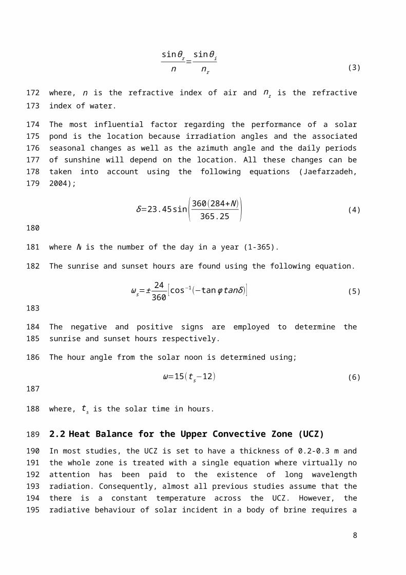
sin θr

n=sin θi

nr (3)

where, n is the refractive index of air and nr is the refractive index of water.

The most influential factor regarding the performance of a solar pond is the location because irradiation angles and the associated seasonal changes as well as the azimuth angle and the daily

5

112

113114

115

116117

118

119120

121

122

123

124125

periods of sunshine will depend on the location. All these changes can be taken into account using the following equations (Jaefarzadeh, 2004);

δ=23.45 sin(360(284+N )365.25 ) (4)

where N is the number of the day in a year (1-365).

The sunrise and sunset hours are found using the following equation.

ωs=± 24360 [cos−1(−tanφ tanδ)] (5)

The negative and positive signs are employed to determine the sunrise and sunset hours respectively.

The hour angle from the solar noon is determined using;

ω=15(t s−12) (6)

where, t s is the solar time in hours.

2.2 Heat Balance for the Upper Convective Zone (UCZ)

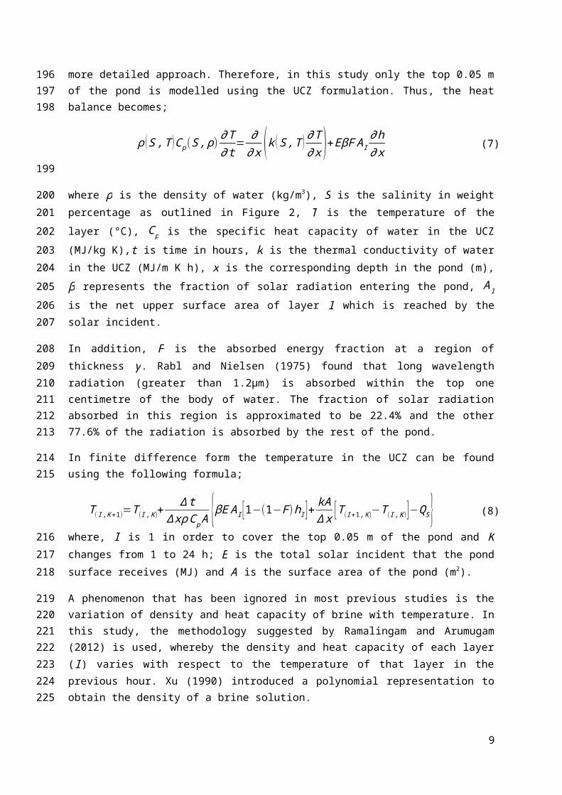
In most studies, the UCZ is set to have a thickness of 0.2-0.3 m and the whole zone is treated with a single equation where virtually no attention has been paid to the existence of long wavelength radiation. Consequently, almost all previous studies assume that the there is a constant temperature across the UCZ. However, the radiative behaviour of solar incident in a body of brine requires a more detailed approach. Therefore, in this study only the top 0.05 m of the pond is modelled using the UCZ formulation. Thus, the heat balance becomes;

ρ (S ,T )Cp(S , ρ)∂T∂t

= ∂∂ x (k (S ,T ) ∂T

∂ x )+EβF A I∂h∂ x (7)

where ρ is the density of water (kg/m3), S is the salinity in weight percentage as outlined in Figure 2, T is the temperature of the layer (°C), C p is the specific heat capacity of water in the UCZ (MJ/kg K),t is time in hours, k is the thermal conductivity of water in the UCZ (MJ/m K h), x is the corresponding depth in the pond (m), β represents the fraction of solar radiation entering the pond, A I is the net upper surface area of layer I which is reached by the solar incident.

In addition, F is the absorbed energy fraction at a region of thickness γ. Rabl and Nielsen (1975) found that long wavelength radiation (greater than 1.2μm) is absorbed within the top one centimetre of the body of water. The fraction of solar radiation absorbed in this region is approximated to be 22.4% and the other 77.6% of the radiation is absorbed by the rest of the pond.

6

126127

128

129

130

131

132133

134

135

136

137

138139140141142143

144

145146147148149

150151152153

In finite difference form the temperature in the UCZ can be found using the following formula;

T (I ,K+1)=T (I , K )+∆t

∆ xρC p A {βE A I [1−(1−F)h I ]+kA∆ x [T (I +1 ,K )−T (I , K )]−QS} (8)

where, I is 1 in order to cover the top 0.05 m of the pond and K changes from 1 to 24 h; E is the total solar incident that the pond surface receives (MJ) and A is the surface area of the pond (m2).

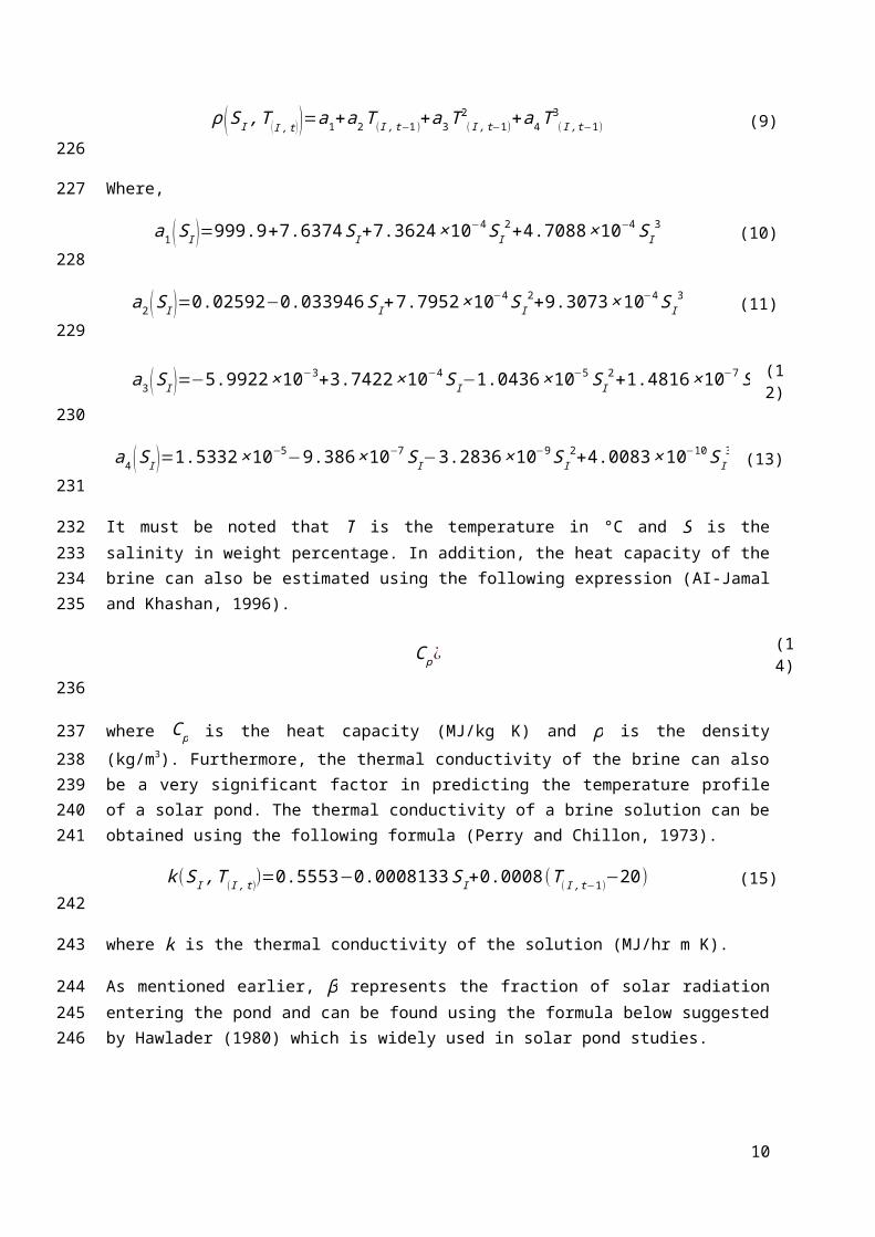
A phenomenon that has been ignored in most previous studies is the variation of density and heat capacity of brine with temperature. In this study, the methodology suggested by Ramalingam and Arumugam (2012) is used, whereby the density and heat capacity of each layer ( I ) varies with respect to the temperature of that layer in the previous hour. Xu (1990) introduced a polynomial representation to obtain the density of a brine solution.

ρ (S I ,T ( I ,t ) )=a1+a2T (I , t−1)+a3T2( I ,t−1 )+a4T

3(I ,t−1) (9)

Where,

a1 (S I )=999.9+7.6374S I+7.3624×10−4 S I

2+4.7088×10−4S I3 (10)

a2 (S I )=0.02592−0.033946S I+7.7952×10−4S I

2+9.3073×10−4S I3 (11)

a3 (S I )=−5.9922×10−3+3.7422×10−4 S I−1.0436×10−5S I

2+1.4816×10−7S I3 (12)

a4 (S I )=1.5332×10−5−9.386×10−7 S I−3.2836×10−9S I

2+4.0083×10−10 S I3 (13)

It must be noted that T is the temperature in °C and S is the salinity in weight percentage. In addition, the heat capacity of the brine can also be estimated using the following expression (AI-Jamal and Khashan, 1996).

C p¿ (14)

where C p is the heat capacity (MJ/kg K) and ρ is the density (kg/m3). Furthermore, the thermal conductivity of the brine can also be a very significant factor in predicting the temperature profile of a solar pond. The thermal conductivity of a brine solution can be obtained using the following formula (Perry and Chillon, 1973).

k (SI , T (I , t))=0.5553−0.0008133S I+0.0008(T (I , t−1)−20) (15)

where k is the thermal conductivity of the solution (MJ/hr m K).

7

154

155156

157158159160161

162

163

164

165

166

167

168169170

171

172173174175

176

177

As mentioned earlier, β represents the fraction of solar radiation entering the pond and can be found using the formula below suggested by Hawlader (1980) which is widely used in solar pond studies.

β=1−0.6[ sin (θi−θ r )sin (θi+θr ) ]

2

−0.4¿¿ (16)

Furthermore, h I denotes the ratio of solar energy reaching layer I to the total solar incident received by the surface. Bryant and Colbeck (1977) suggest that the formula for the effective inclination of the Sun’s rays through the pond and received by layer I is given by Equation 17 which is deduced by considering that the fraction of incident energy after passing through a thickness of x cm of water (depth between 1 centimetre and 10 metre) can be formulated by f ( x )=a−b ln x.

h I=0.727−0.056 ln [ (x−γ )cosθr ] (17)

Where, γ is the thickness of the layer within the UCZ absorbing the long wavelength solar incident (m).

In addition, A I is the net upper surface area of layer I which is reached by the solar incident and can be expressed as (Karakilcik et al., 2006);

A I=LW [LL−(γ+ ( I−1 )∆ x) tanθr ] (18)

where, θr is the refraction angle of solar incident (rad), ∆ x is the thickness of each layer (m), LW and LL are the width and length of the pond (m). The final part of Equation 8, QS, corresponds to the heat losses to the atmosphere (MJ). Detailed analysis of the heat loss from the surface of the pond is presented below.

Heat loss from the surface of the pond occurs due to convection, evaporation, radiation. A model was developed by Kurt et al. (2006) to predict these losses as provided below. Additionally, there is a cooling effect which occurs due to the supply of freshwater to the UCZ. Hence, the total heat loss and in addition to the cooling effect can be calculated by the following procedure.

QS=(Qc+Qe+Qr+Qw¿) A (19)

The convective heat-loss can be determined as follows;

Qc=hc(T I=1−T a) (20)

where T a represents the air temperature at time t of nth day of a year for the city of Adana in southern Turkey (Kayali et al., 1998);

8

178179180

181

182183184185186

187

188189

190191

192

193194195196

197198199200

201

202

203

204205

T a (n ,t )=20+8sin [( 360365 )n−103]+5sin [(36024 ) t ] (21)

Moreover, hc is the wind induced convection heat-transfer coefficient (MJ/hr kg K), which is dependable on the velocity of wind and can be found using;

hc=5.7+3.8V a (22)

where, V a is the wind velocity (m/s). The heat loss caused by evaporation is proportional to the wind-induced convective heat-transfer coefficient hc and the difference between the vapour pressure of the free surface and the partial pressure of the water vapour in the atmosphere. The evaporative heat loss is therefore determined by;

Qe=hc he (Ps−Pamb)1.6CaPatm

(23)

where, he is the latent heat of evaporation (MJ/kg), Ca is the specific heat of air (MJ/kg K), Patm is the atmospheric pressure (Pa) and Ps is the vapour pressure found at the surface temperature (Pa) obtained from the equation below.

Ps=exp(18.403−3885

T I=1+230) (24)

and Pamb is the partial pressure of water vapour in the ambient air and at the ambient temperature (Pa) which is given by;

Pamb=RH exp(18.403−3885

T a+230) (25)

where, RH is relative humidity (%). Moreover, heat loss due to radiation from the surface of the pond to the atmosphere is expressed by;

Qr=εwσ ((T I=1+273.15 )4−(T sky+273.15 )4) (26)

where, εw is the emissivity of water, σ is the Stefan-Boltzman constant (MJ/m2 K4) and T sky is determined by the following formula.

T sky=T a+(0.55+0.704(√Pamb))0.25 (27)

In addition to the above, there will be a cooling effect due to the supply of freshwater to the top of the pond, assumed to be at 25°C, which can be determined using the following procedure.

9

206

207208

209

210211212213

214

215216217

218

219220

221

222223

224

225226

227

228229

Qw¿=GC p fw(T I=1−25) (28)

where, C pfw is defined as the heat capacity of freshwater (MJ/kg K) and G is the rate of evaporation of water (kg/hr) which can be found using the expression below (Finch and Hall, 2006).

G=(25+19V a ) (xs−x ) (29)

Here, xs is the humidity ratio in saturated air and x is the humidity ratio in the air which can be found using the following equation (Gueymard and Kambezidis, 2004).

x=0.62198Pamb

Patm−Pamb(30)

Then, xs can also be calculated (Gueymard and Kambezidis, 2004).

xs=0.62198 Pws

Patm−Pamb(31)

where, Pws is the partial pressure of water in moist air (Pa) and can be determined using the equation below (Osborne and Meyers, 1934).

Pws=2.718

(77.345+(0.0057 T I=1)−7235T I=1

)

T I=18.2

(32)

2.3 Heat Balance for the Non-Convective Zone (NCZ)

The balance for this zone can be expressed as;

ρ (S ,T )Cp(S , ρ( S ,T ))∂T∂t

= ∂∂ x (k (S ,T ) ∂T

∂ x )+Eβ FA I∂h∂ x (33)

Therefore, the layer temperature for the NCZ is given by;

T (I ,K+1)=T (I , K )+∆ t

ρC p A ∆ x {βE A I (1−F )(hI−h I+1)+kA∆x [T ( I+ 1, K )−T ( I , K ) ]− kA

∆ x [T (I , K )−T (I−1 , K)]}(34)

where, I varies from 2 to 14 because the thickness of the NCZ is taken as 0.65 m as shown in Figure 2.

2.4 Heat Balance for the Heat Storage Zone (HSZ)

For this zone, Equation 34 can again be employed to form the energy balance.

10

230

231232

233234235

236

237

238

239240

241

242

243

244

245

246

247248

249

250

ρ (S ,T )Cp(S , ρ( S ,T ))∂T∂t

= ∂∂ x (k (S ,T ) ∂T

∂ x )+EβF A I∂h∂ x (35)

Hence, the temperature of the HSZ will be given by the following equation.

T (I ,K+1)=T (I , K )+∆ t

ρC p A ∆ x {βE A I (1−F )(hI )+kA∆ x [T (I +1 , K )−T ( I , K ) ]− kA

∆ x [T (I , K)−T (I−1 , K )]} (36)

where, I is 15 and the thickness of the HSZ is set to be 0.8 m. As highlighted in Figure 2, in this study the entire heat storage zone is treated as one layer. The rationale behind this approach is that as the salinity is kept constant the temperature will eventually become approximately uniform but a layer-by-layer method will lead to varying values of h I causing fluctuations in temperature across this zone which is unrealistic.

2.5 Heat Balance for the Insulated Bottom Wall (IBW)

The heat balance for the bottom wall is represented by the following expression.

ρinsC pins∂T∂ t

=k ∂2T∂x2

(37)

Hence, the temperature of the IBW layers can be found from the equation below.

T (I ,K+1)b=T (I , K )+∆ t

ρinsCpins A∆ x ins{k ins A∆ x ins

[T (I−1 , K )−T (I ,k )]−k ins A∆xins

[T (I , k)−T ( I+1 , K )]} (38)

The final layer in the insulation beneath the pond exchanges heat with the soil beneath the pond which is assumed to have the same temperature as the air. This assumption is consistent with the results reported by Kayali et al. (1998). The, heat loss from layer 20 is therefore quantified considering the temperature difference between layer 20 and the soil and thermal conductivity of the insulation which is made of glass wool as mentioned previously.

3 Results and discussion

A numerical code was developed using MATLAB R2013a based on the aforementioned procedure for modelling a solar pond. This was carried out using meteorological and solar energy records collected from NASA’s 22 yearlong database (Atmospheric Data Science Center, 2013) considering the city Adana (southern Turkey) as the location. It is assumed that the operation of the pond commences on the first day of June so that the maximum solar radiation can be exploited. The average monthly solar radiation profile of the city of Adana is given in Figure 3.

11

251

252

253

254255256257258

259

260

261

262

263

264265266267268

269

270271272273274275

1 2 3 4 5 6 7 8 9 10 11 120

5

10

15

20

25

30

Month

Sola

r Ene

rgy

(MJ/

m2)

Figure 3: Monthly average solar radiation profile of the city of Adana obtained from Atmospheric Data Science Center.

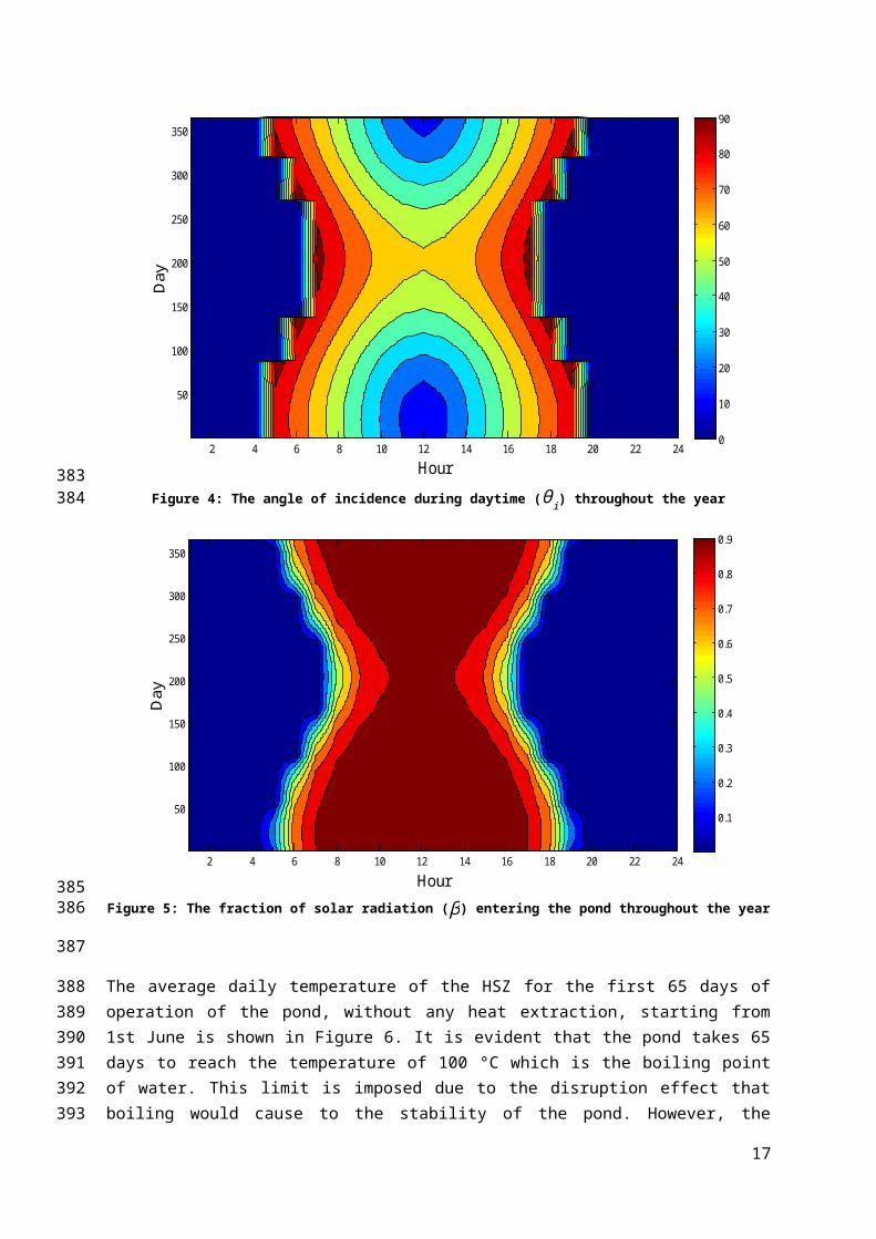
The angle of incidence during daytime (θi) and values for β which is the fraction of solar radiation entering the pond for the entire year are presented in Figures 4 and 5. It is evident that both parameters are at their highest at solar noon (12:00 solar time) throughout the year and the largest values are obtained in the middle of the summer while these values are at their lowest in the middle of the winter. Since the operation of the pond is set to commence on the first day of June, it can be observed that the highest values of θi and β are obtained towards the end of June which is the peak of the summer.

Hour

Day

2 4 6 8 10 12 14 16 18 20 22 24

50

100

150

200

250

300

350

0

10

20

30

40

50

60

70

80

90

Figure 4: The angle of incidence during daytime (θi) throughout the year

12

276277

278

279280281282283284285

286287

Hour

Day

2 4 6 8 10 12 14 16 18 20 22 24

50

100

150

200

250

300

350

0.1

0.2

0.3

0.4

0.5

0.6

0.7

0.8

0.9

Figure 5: The fraction of solar radiation (β) entering the pond throughout the year

The average daily temperature of the HSZ for the first 65 days of operation of the pond, without any heat extraction, starting from 1st June is shown in Figure 6. It is evident that the pond takes 65 days to reach the temperature of 100 °C which is the boiling point of water. This limit is imposed due to the disruption effect that boiling would cause to the stability of the pond. However, the increase in the temperature of the HSZ is not uniform and as the brine gets warmer, it becomes sharper due to the increasing solar radiation intensity and more efficient preservation of heat because of the better establishment of the temperature gradient in the NCZ which will be discussed further. Figure 7 shows that if the operation commences on the first day of December, instead of June, then 82 days will be required to reach 100 °C. This is mainly as a result of less solar radiation, in terms of both intensity and longevity providing heat to the pond as well as lower air temperatures which increase the rate of heat loss. However, the trend on the increase of the temperature is very similar to that of Figure 6. The rest of figures in this section are associated with the 1st June start date.

13

288289

290

291292293294295296297298299300301302

1 5 9 13 17 21 25 29 33 37 41 45 49 53 57 61 6520

30

40

50

60

70

80

90

100

110

Day

Tem

pera

ture

(°C)

Figure 6: The average temperature of the HSZ during the first 65 days of operation of the pond from the 1st June.

1 5 9 13 17 21 25 29 33 37 41 45 49 53 57 61 65 69 73 77 8110

20

30

40

50

60

70

80

90

100

Day

Tem

pera

ture

(°C)

Figure 7: The average temperature of the HSZ during the first 82 days of operation of the pond from the 1st December.

As mentioned previously, this model is accounts for the cooling effect of the supply of freshwater which is added to the surface of the pond in order to replace the evaporated water in the UCZ. Such an effect has seldom been taken into account before. This is crucial in maintaining steady operation of a solar pond as the UCZ exists to ensure the NCZ is stabilised and salinity gradient is preserved. The model described allows the calculation of the amount of water required for every hour of operation. However, as the variation of such amount within a 24-hour period is minimal, the total daily requirement of freshwater is presented in Figure 8. Correspondingly, the quantity of the cooling effect associated with this addition of freshwater is demonstrated in Figure 9.

14

303304

305306

307

308309310311312313314315

1 5 9 13 17 21 25 29 33 37 41 45 49 53 57 61 653839404142434445464748

Day Number

Requ

ired

Fres

hwat

er S

uppl

y (L

itres

)

Figure 8: The volume of freshwater which must be supplied to the LCZ to maintain the volume and stability of the pond during the first 65 days of operation.

Figure 9: The cooling effect (MJ) imposed on the pond due to the continuous supply of freshwater to the UCZ during the first 65 days of operation of the pond.

Approximately 41-47 litres of freshwater needs to be supplied to the UCZ for the first 65 days of operation as indicated in Figure 8. The sharp changes that can be observed on both figures are due to the wind velocity varying from June to July and from July to August as these values are taken as monthly averages. Clearly, the model is sensitive to variation in wind velocity and so could be improved by including daily or hourly averages. However, no such data exists for this location. A general delicate increase can also be observed initially which is due to the increase in the temperature of water that results in growing evaporation from the surface of the pond. However, it has to be noted that the aforementioned continuous cooling effect constitutes a significant fraction of the total loss in comparison with convective heat loss as featured in Figure 10.

15

316317318

319

320321

322

323324325326327328329330331

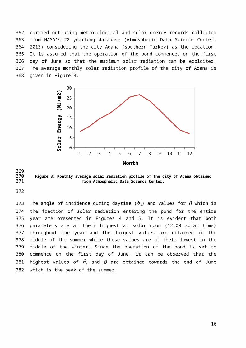
Figure 10: Convective heat loss (MJ) quantities during the first 65 days of operation of the pond.

The quantity of convective heat loss is increases as the temperature of the surface of the pond rises, as would be expected. It can be seen that the convective heat loss declines at sunrise and rises with the sunset. Unsurprisingly, the lowest quantities of the convective heat loss appear to be when the air temperature is at its highest and the highest quantities are when the air temperature is at its lowest. The lowest convective heat loss occurs when the air temperature is at its closest to the temperature of the top layer of the pond ( I=1). However, the effect of convective heat loss is approximately 10 times less than the cooling effect of supply of freshwater to the UCZ in the first 65 days of operation. Hence, the abovementioned cooling effect is crucial to the modelling of a solar pond and must not be overlooked.

The temperature variations in the HSZ during the 48 hours of the pond’s operation until the temperatures reach the boiling point of water (100 °C), in comparison with the temperature variation in days 46 and 47 are illustrated in Figure 11. The corresponding temperatures throughout the pond (all layers) for the same 48-hour periods are then presented in Figures 12 and 13.

16

332333

334

335336337338339340341342343

344345346347

1 5 9 13 17 21 25 29 33 37 41 450

102030405060708090

100

Day 64-65Day 46-47

Hour

Tem

pera

ture

(°C)

Figure 11: The temperature of the HSZ during days 46-47 and 64-65.

Time (Hours)

Laye

r Num

ber

Temperature Distrbution (C)

5 10 15 20 25 30 35 40 45

2

4

6

8

10

12

14 30

35

40

45

50

55

60

65

Figure 12: The temperature across the pond during days 46-47.

Time (Hours)

Laye

r Num

ber

5 10 15 20 25 30 35 40 45

2

4

6

8

10

12

14 50

55

60

65

70

75

80

85

90

95

100

Figure 13: The temperature profile across the pond during days 64-65.

17

348349

350351

352353

The temperature is generally increasing over the 48-hour periods. Since there is no source of energy (radiation), the pond expectedly cools down overnight, as clearly demonstrated by Figures 11, 12 and 13. The difference of approximately 10 °C between day and night particularly in the NCZ and the HSZ are due to the low depth of the pond leading to less insulation provided by the NCZ in addition to the substantial difference between day and night time air temperatures in the location considered in this study. However, owing to the presence of the NCZ and insulation beneath the pond much of the heat is captured by the pond. It is also highlighted that while the HSZ is reaching temperatures close to the boiling point of saturated brine, the temperature in the UCZ is very modest and shows little variation. This is attributed to the heat losses from the surface of the pond as well as the cooling effect of freshwater addition, both of which contribute towards lower temperatures in the UCZ. In addition to that, there is a noteworthy shift in the hottest zone of the pond from the NCZ to the HSZ.

Considering the same 48-hour periods, the surface area ( A I) that the radiation reaches in the HSZ and the fraction of solar energy (h I) reaching the HSZ are shown in Figures 14 and 15, respectively.

1 5 9 13 17 21 25 29 33 37 41 450

102030405060708090

100

Day 46-47Day 64-65

Hour

Area

(m²)

Figure 14: Surface area (A I) that the radiation reaches in the HSZ during days 46-47 and 64-65.

18

354

355356357358359360361362363364365366

367368

369370

371

1 5 9 13 17 21 25 29 33 37 41 450

0.1

0.2

0.3

0.4

0.5

0.6

0.7

0.8

Day 46-47Day 64-65

Hour

Ratio

of S

olar

Ene

rgy

Figure 15: The fraction of solar energy (hI) reaching the HSZ during days 46-47 and 64-65.

In both Figures 14 and 15 it is underlined that the highest values are expectedly obtained at solar noon. Additionally, both A I and h I (very slightly) are higher during days 46-47 than days 64-65 as a result of being closer to middle of the summer which is the peak of solar radiation intensity. The high values of h I reaching the HSZ are due to the low designated depth of the pond. It should also be noted that these are the values of h I for the top of the HSZ and hence the incoming solar energy has to only overcome 0.7 m which leads to high values being obtained.

The average temperature in the insulation underneath the pond is shown in Figure 16. The rise in the temperature in the insulation layers expectedly takes place at a lower rate than the layers within the pond which proves that fibre glass wool performs well in providing thermal protection for a solar pond. Moreover, the rise in temperature becomes sharper as the HSZ gets hotter since the rate of heat transfer between the HSZ and the insulation layers increases.

1 5 9 13 17 21 25 29 33 37 41 45 49 53 57 61 650

5

10

15

20

25

30

35

40

45

Day Number

Tem

pera

ture

(°C)

Figure 16: The average temperature in the insulation layers underneath the pond.

19

372373

374

375376377378379380

381382383384385

386387

The temperature profile throughout the layers of the pond for the 20 days of operation leading to the temperature of 100 °C being reached is displayed in Figure 17. It is illustrated that the HSZ does not immediately become the hottest zone within the pond. However, as the pond starts to get warmer, the hottest zone slowly moves towards the bottom of the pond and settles there. This phenomenon corresponds to the experimental results obtained by several studies (Kurt et al., 2006; Suarez et al. 2014; Li et al. 2000) and defies pseudo-steady state models which assume that the HSZ becomes the hottest zone in a solar pond immediately after the beginning of operation.

Time (Hours)

Laye

r Num

ber

0 50 100 150 200 250 300 350 400 450

2

4

6

8

10

12

14

30

40

50

60

70

80

90

100

Figure 17: Temperature profile for the final 20 days of operation of the pond.

Since most experimental results reported in the literature account for a few days of operation, the stabilisation of the pond is not observed. However, the results presented in this study indicate that after a number of operational days the HSZ will become suitable to extract heat from. The reason behind this movement is that, as explained earlier, 22.4% of the radiation entering the pond is received by the top 1 cm of the pond and due to the salinity gradient, the natural process of heat moving from the top to bottom due to the salinity gradient occurs. It must be noted that the profile is only applicable to the start-up process of a solar pond and after the establishment of temperature gradient, the HSZ stays as the hottest section of the pond.

The other occurrence that can be deduced from Figure 17 is that as the temperature increases and edges closer to the boiling point, the pond performs better in terms of preserving the accumulated heat and heat losses overnight become less significant. This is due to the better establishment of the temperature gradient in the NCZ leading to more efficient insulation of the HSZ.

4 Conclusions

A comprehensive model has been developed to include many parameters affecting a solar pond using a finite difference method which has been modified so that the HSZ is treated as one layer with

20

388

389390391392393394395

396397

398

399400401402403404405406

407408409410

411

412413

uniform temperature in addition to heat losses from the surface of the pond as well as the cooling effect due to the freshwater supplied to the surface of the pond being incorporated. The presented model can be used to simulate solar ponds of various dimensions and for any given location. This is a transient model for the simulation of a solar pond from the very start of operation which can predict the temperature of brine in any layer on an hourly basis. The model provides a comprehensive method comprising various previously developed formulations.

It was found that there is a sharp increase in the temperature of the UCZ due to long wavelength radiation being absorbed within the top 1 cm and therefore a constant temperature does not exist in the UCZ which defies the assumption that is made by most studies. If the operation starts on the first day of June, the simulated 100 m2 pond takes 65 days until it reaches 100 °C. This would be 82 days if the operation was to start on the first day of December. The difference is predominantly due to a lesser quantities of solar radiation reaching the surface of the pond and lower air temperatures.

The cooling effect of freshwater supply to the UCZ is approximately 10 times larger than the convective heat loss from the surface of the pond in the first 65 days of operation and therefore must always be accounted for in solar pond modelling studies.

The HSZ does not immediately become the hottest zone within the pond. However, as the temperature increases and the pond edges closer to pseudo-steady state, the hottest zone slowly moves towards the HSZ and settles there which is consistent with experimental results obtained by several studies. As the temperature increases in the HSZ, it becomes more resistant to losing the accumulated heat due to the establishment of the temperature gradient in the NCZ leading to better insulation of the HSZ.

Furthermore, while the temperature in the HSZ exceeds 100°C, modest temperatures of 50-60 °C exist in the UCZ as a consequence of heat losses from the surface and the cooling effect of freshwater supply to the UCZ.

Further studies must be carried out to incorporate the process of heat extraction from the solar pond and examine the associated effects of various extraction methods on the temperature profile.

Acknowledgments

The financial support of the Chemical and Process Engineering Department at the University of Surrey is gratefully acknowledged.

References

AI-Jamal, K., Khashan, S., 1996, Parametric Study of Solar Pond in Northern Jordan, Energy 21 (1996) 939–946.

Akbarzadeh, A., Andrews, J., Golding, P., 2005, Solar pond technologies: a review and future directions in Y. Goswami (ed.) Advances in Solar Energy, Earthscan, London, UK, pp. 233–294.

21

414415416417418419

420421422423424425

426427428

429430431432433434

435436437

438439

440

441442

443

444445

446447

Atmospheric Data Science Center, Surface Meteorology and Solar Energy, NASA, USA, Available at: https://eosweb.larc.nasa.gov/sse/, [Accessed on 15/10/2013].

Bansal, P.K., Kaushik, N.D., 1981, Salt gradient stabilized solar pond collector, Energy Conversion and Management 21 (1981) 81–95.

Beniwal, R.S., Singh, R.V., Chaudhary, D.R., 1985, Heat losses from a salt-gradient solar pond, Applied Energy 19 (1985) 273–285.

Bernad, F., Casas, S., Gibert, O., Akbarzadeh, A., Cortina, J.L., Valderrama, C., 2013. Salinity gradient solar pond: validation and simulation model, Solar Energy 98 (2013) 366–374.

Bryant, H.C., Colbeck, I., 1977, A solar pond for London, Solar Energy 19 (1977) 321–322.

Duffle, J.A., Beckman, W.E., Solar Engineering of Thermal Processes, Wiley, New York, 1980.

Earth System NOAA Earth System Research Laboratory/Global Monitoring Division, 2013, USA.

Finch, J.W., Hall, R.L., 2006, Evaporation from lakes. In: Anderson, M.G. (Ed.), Encyclopedia of Hydrological Sciences, John Wiley & Sons.

Gueymard, C.A., Kambezidis, H.D., 2004, Solar radiation and daylight models. In Muneer, T. (Ed.), Amsterdam: Elsevier.

Hawlader, M.N.A., Brinkworth, B.J., 1981, An analysis of the non convecting solar pond. Solar Energy, 27 (1981) 195–204.

Hawlader, M.N.A., 1980, The influence of the extinction coefficient on the effectiveness of solar ponds, Solar Energy 25 (1980) 461–464.

Hull, J.R., 1980, Computer simulation of solar pond thermal behaviour, Solar Energy 25 (1980) 33–40.

International Energy Outlook, 2014, U.S. Energy Information Administration, Washington DC, USA.

Jaefarzadeh, M.R., 2004, Thermal behavior of a small salinity-gradient solar pond with wall shading effect, Solar Energy 77 (2004) 281–290.

Jaefarzadeh, M.R., Akbarzadeh, A., 2002, Towards the design of low maintenance salinity gradient solar ponds, Solar Energy 73 (2002) 375–384.

Karakilcik, M., Dincer, I., Rosen, M.A., 2006, Performance investigation of a solar pond, Applied Thermal Engineering 26 (2006) 727–735.

Karakilcik, M., Kıymac, K., Dincer, I., 2006, Experimental and theoretical temperature distributions in a solar pond, International Journal of Heat and Mass Transfer 49 (2006) 825–835.

Kayali, R., Bozdemir, S., Kiymac, K., 1998, A rectangular solar pond model incorporating empirical functions for air and soil temperatures, Solar Energy 63 (1998) 345–353.

Kooi, C.F., 1979, The steady state salt gradient solar pond, Solar Energy 23 (1979) 37–45.

22

448449

450451

452453

454455

456

457

458

459460

461462

463464

465466

467

468

469470

471472

473474

475476

477478

479

Kurt H., Ozkaymak, M., Binark, A.K., 2006, Experimental and numerical analysis of sodium-carbonate salt-gradient solar pond performance under simulated solar radiation. Applied Energy 83 (2006) 324–342.

Li, X.Y., Kanayama, K., Baba, H., 2000, Spectral calculation of the thermal performance of a solar pond and comparison of the results with experiments, Renewable Energy 20 (2000) 371–387.

Mazidi, M., Shojaeefard, M.H., Mazidi, M.S., Shojaeefard, H., 2011, Two-dimensional modeling of a salt gradient solar pond with wall shading effect and thermo-physical properties dependent on temperature and concentration. Thermal Science 20 (4), 362–370.

Osborne, N.S., Meyers, C.H., 1934, A formula and tables for the pressure of saturated water vapor in the range 0 to 374°C, l. Research NBS 13, 1 (1934).

Own, S.H., Ambel, A.B., 1982, Net energy analysis of residential solar ponds, Energy 7 (1982) 457–463.

Perry, R., Chillon, C., Chemical Engineering Handbook, 5th edn., McGraw-Hill, New York, 1973.

Rabl, A., Nielsen, C.F., 1975, Solar pond for space heating, Solar Energy 17(1975) 1–12.

Ramalingam, A., Arumugam, S., 2012, Experimental Study on Specific Heat of Hot Brine for Salt Gradient Solar Pond Application, International Journal of ChemTech Research, Vol.4, No.3, pp 956–961, July-Sept 2012.

Rubin, H., Benedict, B.A., Bachu, S., 1984, Modeling the performance of a solar pond as a source of thermal energy, Solar Energy, 32 (1984) 771–778.

Sakhrieh, A., Al-Salaymeh, A., 2013, Experimental and numerical investigations of salt gradient solar pond under Jordanian climate conditions, Energy Conversion and Management 65 (2013) 725–728.

Sodha, M.S., Kaushik, N.D., Rao, S.K., 1981, Thermal analysis of three zone solar pond, Energy Research 5 (1981) 321–340.

Suárez F., Tyler S.W., Childress A.E., 2010, A fully coupled transient double-diffusive convective model for salt-gradient solar ponds, International Journal of Heat and Mass Transfer 53 (2010) 1718–1730.

Suarez, F., Ruskowitz, J.A., Childress, A.E, Tyler, S. W., 2014, Understanding the expected performance of large-scale solar ponds from laboratory-scale observations and numerical modeling, Applied Energy 117 (2014) 1–10.

Tabor, H., Doron, B., 1986, Solar Ponds-lesson learned from the 150 KWe power plant at Ein Boqek. In: Proceedings of ASME Solar Energy Division, Anaheim, CA.

Velmurugana, V., Srithar, K., 2008, Prospects and scopes of solar pond: A detailed review, Renewable and Sustainable Energy Reviews 12 (2008) 2253–2263.

Xu, H., 1990, Laboratory Studies on Dynamical Processes in Salinity Gradient Solar Pond. PhD Thesis, The Ohio State University, USA.

23

480481482

483484

485486487

488489

490491

492

493

494495496

497498

499500

501502

503504505

506507508

509510

511512

513514