Predicting the Effectiveness of Partial Evaluation

German Vidal

Technical University of Valencia, Spain.gvidal@dsic.upv.es

Abstract. Partial evaluation aims at improving programs by special-izing them w.r.t. part of their input data. In general, however, the ef-fectiveness of the partial evaluation process is hard to measure, even aposteriori. Recent approaches have introduced experimental (often com-putationally expensive) frameworks for this purpose.

In this paper, we present an alternative, symbolic approach for predictingthe effectiveness of partial evaluation by combining a trace analysis witha termination analysis. The termination analysis—namely, a size-changeanalysis—is used to determine which procedures are potentially remov-able by partial evaluation (i.e., can be fully unfolded at specializationtime). Then, the trace analysis helps us to put this information into con-text by producing a compact representation of the call sequences of theprogram. By inspecting the output of the combined analysis, the usermay determine the impact of a partial evaluation before it is performed.

1 Introduction

The main goal of partial evaluation [18] is program specialization. Essentially,given a program and part of its input data—the so called static data—a partialevaluator returns a new, residual program which is specialized for the givendata. In the optimal case, all operations that depend only on the static data areperformed once and for all during partial evaluation. An appropriate residualprogram for executing the remaining computations—those that depend on theso called dynamic data—is thus the output of the partial evaluator.

Among the different techniques for program specialization, partial evalua-tion is likely the one which has achieved a higher level of automation. However,despite the fact that the main goal of partial evaluation is improving program ef-ficiency (i.e., producing faster programs), there are very few approaches devotedto formally analyze the effects of partial evaluation, either a priori (prediction)or a posteriori. Recent approaches (e.g., [11, 27]) have considered experimentalframeworks for estimating the best division (roughly speaking, a classificationof program parameters into static or dynamic), so that the optimal choice isfollowed when specializing the source program. The main drawback of theseapproaches, however, is that they are often computationally expensive since anumber of testing partial evaluations (though for simpler test cases) should bemade in order to determine the best division.

/.-,()*+sl

sl

???

???

/.-,()*+ /.-,()*+add

add

mm

/.-,()*+sl2

OO

(a)

/.-,()*+sl

sl

???

???

/.-,()*+ /.-,()*+add

PP

add

mm

(b)

/.-,()*+sl

sl

mm

/.-,()*+

(c)

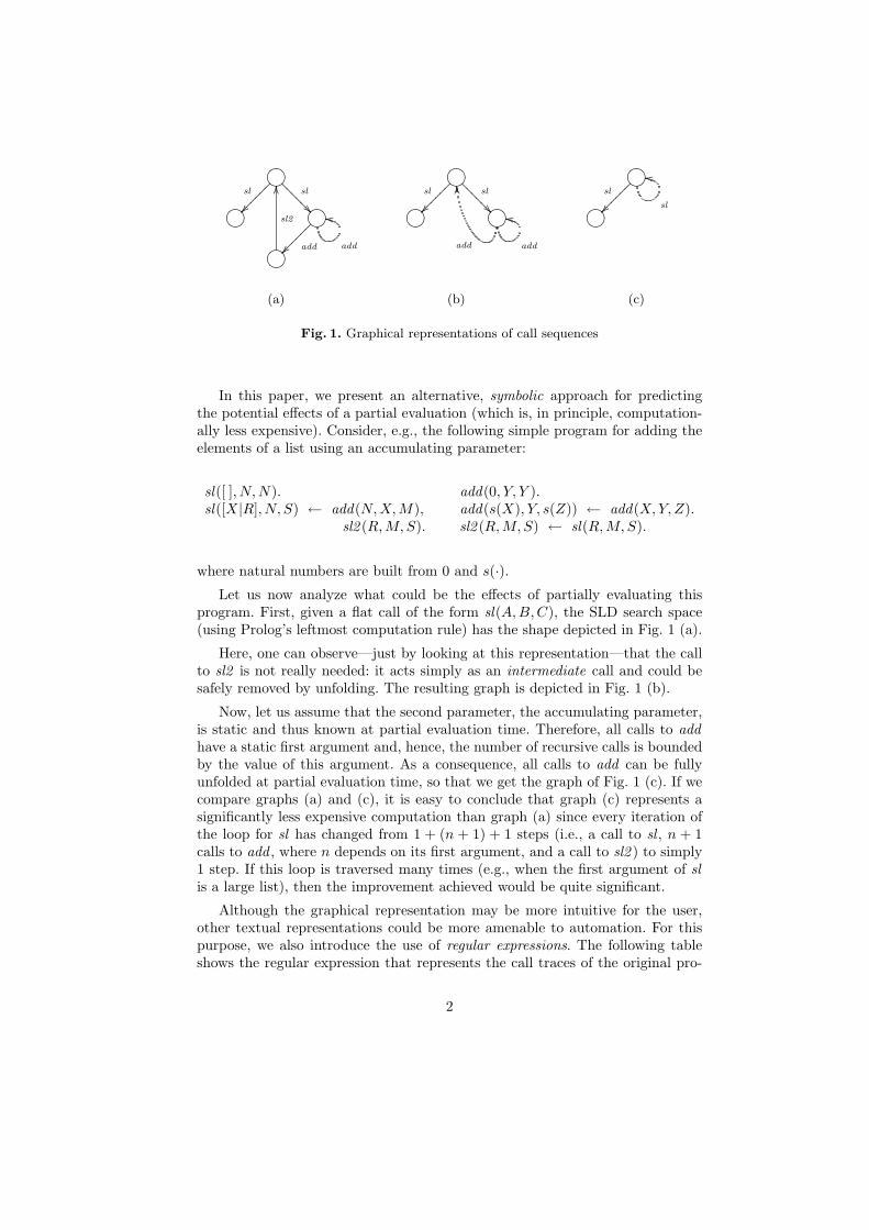
Fig. 1. Graphical representations of call sequences

In this paper, we present an alternative, symbolic approach for predictingthe potential effects of a partial evaluation (which is, in principle, computation-ally less expensive). Consider, e.g., the following simple program for adding theelements of a list using an accumulating parameter:

sl([ ], N, N). add(0, Y, Y ).sl([X|R], N, S) ← add(N,X,M), add(s(X), Y, s(Z)) ← add(X, Y, Z).

sl2 (R,M, S). sl2 (R,M, S) ← sl(R,M, S).

where natural numbers are built from 0 and s(·).Let us now analyze what could be the effects of partially evaluating this

program. First, given a flat call of the form sl(A,B, C), the SLD search space(using Prolog’s leftmost computation rule) has the shape depicted in Fig. 1 (a).

Here, one can observe—just by looking at this representation—that the callto sl2 is not really needed: it acts simply as an intermediate call and could besafely removed by unfolding. The resulting graph is depicted in Fig. 1 (b).

Now, let us assume that the second parameter, the accumulating parameter,is static and thus known at partial evaluation time. Therefore, all calls to addhave a static first argument and, hence, the number of recursive calls is boundedby the value of this argument. As a consequence, all calls to add can be fullyunfolded at partial evaluation time, so that we get the graph of Fig. 1 (c). If wecompare graphs (a) and (c), it is easy to conclude that graph (c) represents asignificantly less expensive computation than graph (a) since every iteration ofthe loop for sl has changed from 1 + (n + 1) + 1 steps (i.e., a call to sl , n + 1calls to add , where n depends on its first argument, and a call to sl2 ) to simply1 step. If this loop is traversed many times (e.g., when the first argument of slis a large list), then the improvement achieved would be quite significant.

Although the graphical representation may be more intuitive for the user,other textual representations could be more amenable to automation. For thispurpose, we also introduce the use of regular expressions. The following tableshows the regular expression that represents the call traces of the original pro-

2

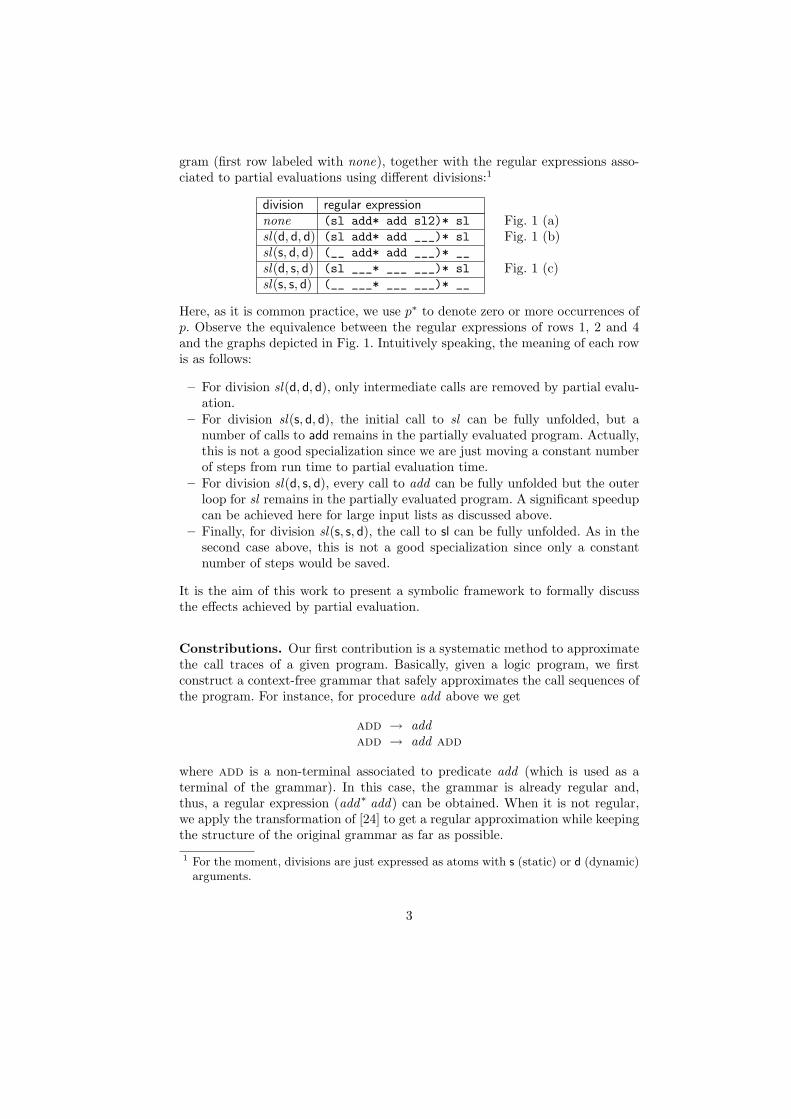
gram (first row labeled with none), together with the regular expressions asso-ciated to partial evaluations using different divisions:1

division regular expressionnone (sl add* add sl2)* sl Fig. 1 (a)sl(d, d, d) (sl add* add ___)* sl Fig. 1 (b)sl(s, d, d) (__ add* add ___)* __sl(d, s, d) (sl ___* ___ ___)* sl Fig. 1 (c)sl(s, s, d) (__ ___* ___ ___)* __

Here, as it is common practice, we use p∗ to denote zero or more occurrences ofp. Observe the equivalence between the regular expressions of rows 1, 2 and 4and the graphs depicted in Fig. 1. Intuitively speaking, the meaning of each rowis as follows:

– For division sl(d, d, d), only intermediate calls are removed by partial evalu-ation.

– For division sl(s, d, d), the initial call to sl can be fully unfolded, but anumber of calls to add remains in the partially evaluated program. Actually,this is not a good specialization since we are just moving a constant numberof steps from run time to partial evaluation time.

– For division sl(d, s, d), every call to add can be fully unfolded but the outerloop for sl remains in the partially evaluated program. A significant speedupcan be achieved here for large input lists as discussed above.

– Finally, for division sl(s, s, d), the call to sl can be fully unfolded. As in thesecond case above, this is not a good specialization since only a constantnumber of steps would be saved.

It is the aim of this work to present a symbolic framework to formally discussthe effects achieved by partial evaluation.

Constributions. Our first contribution is a systematic method to approximatethe call traces of a given program. Basically, given a logic program, we firstconstruct a context-free grammar that safely approximates the call sequences ofthe program. For instance, for procedure add above we get

add → addadd → add add

where add is a non-terminal associated to predicate add (which is used as aterminal of the grammar). In this case, the grammar is already regular and,thus, a regular expression (add∗ add) can be obtained. When it is not regular,we apply the transformation of [24] to get a regular approximation while keepingthe structure of the original grammar as far as possible.

1 For the moment, divisions are just expressed as atoms with s (static) or d (dynamic)arguments.

3

Our second contribution is a method for determining how a given divisionmay affect the program loops. For this purpose, we consider the size-changeanalysis of [31]. The relevance of this analysis (in contrast to other terminationanalysis) is that it is independent of the computation rule (which may allow muchfaster partial evaluation, as shown in [20] in the context of the partial evaluatorLogen [19]). This is a requirement in our setting since partial evaluation oftenconsiders liberal selection policies that depend on the available information (e.g.,only calls which are instantiated enough to ensure finite unfolding are unfolded).

Once size-change analysis has identified the (potential) loops of the program,we use the information provided by a division in order to determine which loopscan be safely unfolded. As a consequence, the output of the trace analysis (e.g., aregular expression denoting the possible sequences of calls) is modified in order toreflect the elimination of these loops. In this paper, we focus on providing simpleand useful information for the user in order to analyze the effects of differentpartial evaluations. Nonetheless, an automated analysis of the associated regularexpressions is also possible, though it is outside the scope of this paper.

The paper is organized as follows. After introducing some preliminaries in thenext section, we present our stepwise transformation for approximating the calltraces of logic programs in Sect. 3. Then, in Sect. 4, we recall the fundamentalsof size-change analysis and use the output of this analysis for estimating theeffects of partial evaluation w.r.t. a given division; we also present some detailsof a prototype implemention as well as a number of experimental results. Finally,Sect. 5 discusses some related work and Sect. 6 concludes and presents severalpossibilities for future work.

2 The Language

We consider a first-order language with a fixed vocabulary of predicate symbols,function symbols, and variables denoted by Π, F and V, respectively. We letT (F ,V) denote the set of terms constructed using symbols from F and variablesfrom V. An atom has the form p(t1, . . . , tn) with p/n ∈ Π and ti ∈ T (F ,V) fori = 1, . . . , n. A query is a finite sequence of atoms 〈A1, . . . , An〉, where theempty query is denoted by true. A clause has the form H ← B1, . . . , Bn whereH,B1, . . . , Bn, n > 0, are atoms (i.e., we only consider definite programs). Alogic program is a finite sequence of clauses. Var(s) denotes the set of variablesin the syntactic object s (i.e., s can be either a term, an atom, a query, or aclause). A syntactic object s is ground if Var(s) = ∅.

Substitutions and their operations are defined as usual. In particular, theset Dom(σ) = x ∈ V | σ(x) 6= x is called the domain of a substitution σ. Asyntactic object s1 is more general than a syntactic object s2, denoted s1 6 s2,if there exists a substitution θ such that s2 = s1θ. The most general unifier oftwo syntactic objects, s1 and s2, denoted by mgu(s1, s2), is a unifier of s1 ands2 which is more general than any other unifier of s1 and s2.

Computations in logic programming are formalized by means of SLD res-olution. The notion of computation rule R is used to select an atom within

4

a query for its evaluation. Given a program P , a query Q = 〈A1, . . . , An〉,and a computation rule R, we say that Q ;P,R,σ Q′ is an SLD resolutionstep for Q with P and R if R(Q) = Ai, 1 6 i 6 n, is the selected atom,H ← B1, . . . , Bm is a renamed apart clause of P , σ = mgu(A,H), and Q′ =(〈A1, . . . , Ai−1, B1, . . . , Bm, Ai+1, . . . , An〉)σ; we often omit P , R and/or σ inthe notation of an SLD resolution step when they are clear from the context.An SLD derivation is a (finite or infinite) sequence of SLD resolution steps.We often use Q0 ;∗

θ Qn as a shorthand for Q0 ;θ1 Q1 ;θ2 . . . ;θn Qn withθ = θ1· · ·θn (where θ = if n = 0). An SLD derivation Q ;∗

θ Q′ is successfulwhen Q′ = true; in this case, we say that θ is the computed answer substitution.SLD derivations are represented by a (possibly infinite) finitely branching tree.

3 Trace Analysis for Logic Programs

In this section, we aim at capturing the shape of a computation by producing afinite representation of all possible sequences of predicate calls.

For this purpose, we introduce a stepwise method that starts with a context-free grammar (CFG) that approximates the call sequences of a logic program(LP), which is then approximated by a strongly regular grammar (SRG), ifneeded, and transformed into a finite automaton (FA) whose accepted languagecan be represented by means of a regular expression (ER). Graphically: LP ⇒ CFG ⇒ SRG ⇒ FA ⇒ RE

The next sections formalize this process.

3.1 From Logic Programs to Context-Free Grammars

Let us first formalize our notion of call trace. For the sake of clarity, we assumein the following that programs do not contain occurrences of the same predicatename with different arities.2

Furthermore, we consider a fixed computation rule for call traces, namelyProlog’s leftmost computation rule, which we denote by Rleft .3 In what follows,we often label SLD resolution steps with the predicate symbol of the selectedatom, i.e., we write Q0

p0; Q1

p1; . . . with pred(Rleft(Qi)) = pi, i ≥ 0, where

pred(A) returns the predicate symbol of atom A.

Definition 1 (call trace). Let P be a program and Q0 a query. We say thatτ = p0 p1 . . . pn−1 ∈ Π∗, n ≥ 1, is a call trace for Q0 with P iff there exists asuccessful SLD derivation Q0

p0; Q1

p1; . . .

pn−1; Qn.

2 This is not a real restriction and, indeed, it is not required in the implemented tool(where predicate names are simply suffixed with their arity).

3 Note that we assume Rleft only at run time, but allow arbitrary computation rulesat partial evaluation time.

5

The first step of our trace analysis consists in producing a context-free gram-mar (CFG) associated to the considered program. A CFG G is a tuple G =〈Σ,N,R, S〉, where Σ and N are two finite disjoint set of terminals and non-terminals, respectively, S ∈ N is the start symbol, and R is a finite set of rules.Each rule has the form A→ α with A ∈ N and α ∈ V ∗, where V denotes Σ∪N .The relation → on N × V ∗ is extended to a relation on V ∗ × V ∗ in the usualway. The transitive and reflexive closure of→ is denoted by→∗. The context-freelanguage generated by G is given by L(G) = w | Σ∗ | S →∗ w. See, e.g., [17]for more details on CFGs.

In the following, given a predicate symbol p ∈ Π, we denote by p 6∈ Π a freshsymbol representing the non-terminal associated to p. Furthermore, we denoteby pred(A) the non-terminal associated to the predicate symbol of atom A, i.e.,pred(A) = p if A = p(t1, . . . , tn). Also, we let Π denote the set p | p ∈ Πof non-terminals associated to predicate symbols. In contrast, we directly usepredicate symbols from Π as terminals.

We let start be a fresh symbol not in Π ∪ Π which we use as a genericstart symbol for CFGs. Given a program and a predicate symbol, we constructan associated CFG, called trace CFG, as follows:

Definition 2 (trace CFG, cfgPq ). Let P be a program and q ∈ Π a predicate

symbol with associated non-terminal q. The associated trace CFG is cfgPq =

〈Π,Π ∪ start, R, start〉, where the set of rules R is defined as follows:

start→ q∪

pred(A0)→ pred(A0)pred(B1) . . .pred(Bn) | A0 ← B1, . . . , Bn ∈ P, n ≥ 0

Roughly speaking, the trace CFG associated to a logic program mimics theexecution of the original program

– by replacing queries (sequences of atoms) by sequences of non-terminals and– by producing a terminal with the predicate symbol of the selected atom at

each SLD-resolution step.

Clearly, the trace CFG may produce call traces that are not possible in theassociated logic program because the “propositional” approximation that formsthe basis of trace CFGs clearly involves a loss of accuracy (consider, e.g., thatnot all atoms with the same predicate symbol unify).

As a counterpart, the generation of the trace CFG can be done very efficientlysince only a single pass over the associated logic program is required.

6

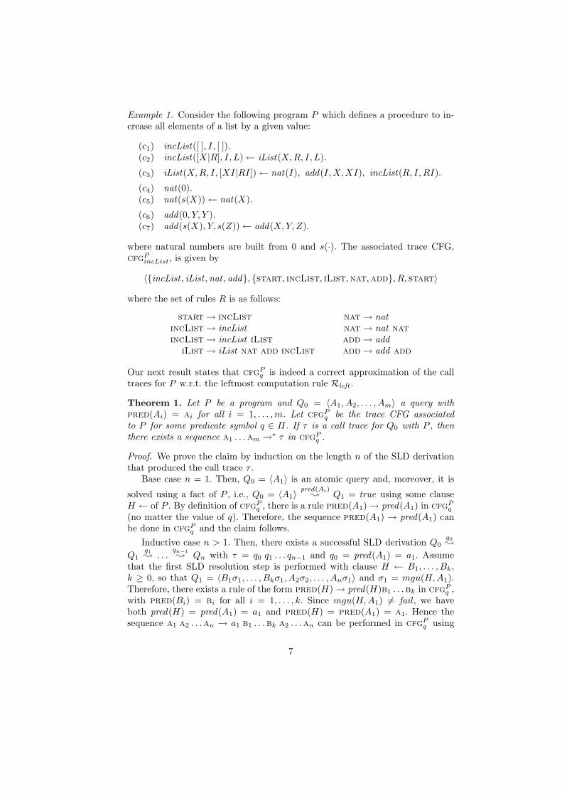
Example 1. Consider the following program P which defines a procedure to in-crease all elements of a list by a given value:

(c1) incList([ ], I, [ ]).(c2) incList([X|R], I, L)← iList(X, R, I, L).

(c3) iList(X, R, I, [XI|RI])← nat(I), add(I,X,XI), incList(R, I,RI).

(c4) nat(0).(c5) nat(s(X))← nat(X).

(c6) add(0, Y, Y ).(c7) add(s(X), Y, s(Z))← add(X, Y, Z).

where natural numbers are built from 0 and s(·). The associated trace CFG,cfgP

incList, is given by

〈incList , iList ,nat , add, start, incList, iList,nat,add, R, start〉

where the set of rules R is as follows:

start→ incList nat→ natincList→ incList nat→ nat natincList→ incList iList add→ add

iList→ iList nat add incList add→ add add

Our next result states that cfgPq is indeed a correct approximation of the call

traces for P w.r.t. the leftmost computation rule Rleft .

Theorem 1. Let P be a program and Q0 = 〈A1, A2, . . . , Am〉 a query withpred(Ai) = ai for all i = 1, . . . ,m. Let cfgP

q be the trace CFG associatedto P for some predicate symbol q ∈ Π. If τ is a call trace for Q0 with P , thenthere exists a sequence a1 . . .am →∗ τ in cfgP

q .

Proof. We prove the claim by induction on the length n of the SLD derivationthat produced the call trace τ .

Base case n = 1. Then, Q0 = 〈A1〉 is an atomic query and, moreover, it is

solved using a fact of P , i.e., Q0 = 〈A1〉pred(Ai)

; Q1 = true using some clauseH ← of P . By definition of cfgP

q , there is a rule pred(A1)→ pred(A1) in cfgPq

(no matter the value of q). Therefore, the sequence pred(A1) → pred(A1) canbe done in cfgP

q and the claim follows.Inductive case n > 1. Then, there exists a successful SLD derivation Q0

q0;

Q1q1; . . .

qn−1; Qn with τ = q0 q1 . . . qn−1 and q0 = pred(A1) = a1. Assume

that the first SLD resolution step is performed with clause H ← B1, . . . , Bk,k ≥ 0, so that Q1 = 〈B1σ1, . . . , Bkσ1, A2σ2, . . . , Anσ1〉 and σ1 = mgu(H,A1).Therefore, there exists a rule of the form pred(H)→ pred(H)b1 . . .bk in cfgP

q ,with pred(Bi) = bi for all i = 1, . . . , k. Since mgu(H,A1) 6= fail , we haveboth pred(H) = pred(A1) = a1 and pred(H) = pred(A1) = a1. Hence thesequence a1 a2 . . .an → a1 b1 . . .bk a2 . . .an can be performed in cfgP

q using

7

rule a1 → a1 b1 . . .bk. Now, consider the SLD derivation Q1 ; . . . ; Qn

with associated call trace τ ′. By the inductive hypothesis, we have that the se-quence pred(B1σ1) . . .pred(Bkσ1)pred(A2σ2) . . .pred(Anσ1) →∗ τ ′ can beperformed with the rules of cfgP

q . Finally, since pred(A) = pred(Aσ) andpred(A) = pred(Aσ) for all atom A and substitution σ, the claim followsfrom a1 a2 . . .an → a1 b1 . . .bk a2 . . .an and b1 . . .bk a2 . . .an →∗ τ ′.

The next corollary is an straightforward consequence of Theorem 1:

Corollary 1. Let P be a program and Q0 = 〈q(t1, . . . , tn)〉 an atomic query. LetΩ be the (possibly infinite) set of call traces for Q0 with P . Then Ω ⊆ L(cfgP

q ).

3.2 Approximating Trace CFGs

Unfortunately, trace CFGs do not always allow us to produce a simple andcompact representation of the call traces of a program (e.g., when the associatedlanguages are not regular). In this section, we use the transformation from [24]to approximate a trace CFG with a strongly regular grammar (SRG).4 Therelevance of SRGs is that they can be mapped to equivalent finite-state automatausing an efficient algorithm. Moreover, the transformation of [24] guarantees thatthe result remains readable and mainly preserves the structure of the originalCFG.

Given a CFG, the first step of the transformation consists in computing thesets of mutually recursive non-terminals. This can be done in linear time in thesize of the CFG by, e.g., computing the strongly connected components of thegraph of the grammar.5

A grammar is called left-linear if every rule has either the form

A→ t or A→ t B

where t is a finite sequence of terminals and A,B are non-terminals. The follow-ing definition is slightly adapted from [24] to the case of trace CFGs:

Definition 3 (trace SRG, srgPq ). Let P be a program, q ∈ Π a predicate

symbol, and cfgPq = 〈Π,Π ∪ start, R, start〉 the trace CFG for P and q. The

associated trace SRG, in symbols srgPq , is obtained from cfgP

q as follows:

– First, we compute the set of mutually recursive non-terminals of cfgPq .

– Then, for each set M of mutually recursive non-terminals such that the rulesdefining these non-terminals are not all left-linear w.r.t. the non-terminalsof M ,6 we apply a grammar transformation as follows:

4 SRGs coincide with the class of grammars without self-embedding [8].5 The graph of a grammar contains one node for each non-terminal and an edge from

node A to node B if non-terminal B appears in the right-hand side of a rule withleft-hand side A.

6 This condition relaxes the standard notion of left-linear grammar by consideringnon-terminals from (Π \M) as terminals.

8

1. For each non-terminal A ∈M , we introduce a fresh non-terminal A′ andadd the following rule to the grammar:7

A′ → ε

2. For each non-terminal A ∈M and each rule

A→ t0 B1 t1 B2 t2 . . . Bm tm

with m ≥ 0, B1, . . . , Bm ∈ M , t0, . . . , tm ∈ (Π ∪ (Π \M))∗, we replacethis rule by the following set of rules:

A → t0 B1

B′1 → t1 B1

B′2 → t2 B3

. . .B′

m−1 → tm1 Bm

B′m → tm A′

(Note that this set reduces to A→ t0 A′ when m = 0.)– Finally, we let srgP

q = 〈Π,Π ∪N ∪start, R′, start〉, where R′ is the set ofrules that results from R by applying the process above and N are the freshnon-terminals added during this process.

According to [24], the transformed grammar srgPq is strongly regular and can

be compiled into a finite automaton in linear time by existing algorithms. Fur-thermore, the language generated by the transformed grammar is a superset ofthat of the original grammar [24], i.e., L(srgP

q ) ⊇ L(cfgPq ) for all program P

and predicate symbol q, which means (by Corollary 1) that srgPq is a complete

approximation of all call traces for P .

Example 2. Consider the cfgPq of Example 1. The sets of mutually recursive

non-terminals areincList, iList, nat, add

Since the rules for nat and add are left-linear, we focus on the set M =incList, iList. Here, the only potentially non-linear rule is

iList→ iList nat add incList

However, since nat,add 6∈ M , this rule is considered left-linear w.r.t. M andneeds not be replaced. Therefore, in this case, we have cfgP

incList = srgPincList .

Example 3. Consider the following program P defining multiplication and addi-tion on natural numbers:

mult(0, Y, 0).mult(s(X), Y, Z)← mult(X, Y, Z1), add(Z1, Y, Z).

add(0, Y, Y ).add(s(X), Y, s(Z))← add(X, Y, Z).

7 We denote by ε the empty sequence.

9

The trace grammar cfgPmult contains the following rules:

start→ mult mult→ mult add→ addmult→ mult mult add add→ add add

The sets of mutually recursive non-terminals are mult, add. While therules for add are clearly left-linear, the second rule of mult is not left-linearbecause, even if add is treated as a terminal, it appears to the right of thenon-terminal mult. Here, srgP

mult will contain the following set of rules:

start→ mult mult → mult mult′ add→ addmult′ → ε mult → mult mult add→ add add

mult′ → add mult′

3.3 A Compact Representation for Call Traces

Once we have a SRG that safely approximates the call traces of a program, thereare several possibilities for representing the language generated by this SRG ina compact and intuitive way. Here, we consider the generation of a finite-stateautomaton (FA) that accepts the language generated by the SRG as well as aregular expression (RE) that represents this language.

Trace Finite Automata. A finite-state automaton (FA) is specified by a tuple〈Q,Σ, δ, s0, F 〉, where Q is a finite set of states, Σ is an input alphabet, δ ⊆Q×Σ ×Q is a (finite) set of transitions, s0 ∈ Q is the start state and F ⊆ Q isa set of final states. For constructing a finite automaton FA(G) from a SRG G,we follow the classical approach from [1] (though more refined methods exist,see, e.g., [26, 25]). Intuitively speaking, we proceed as follows:

– There is a start state in the FA associated to the start symbol of the SRG.– Then, for each reduction w → w′ using a rule A→ t B of the SRG, we have

a transition (s, α, s′) in the FA. States s, s′ are associated with the sequenceof non-terminals in w,w′ (so that if the same sequence occurs more thanonce, the same state is used). The character α is set to the sequence t in theapplied rule (see [1] for a detailed description).

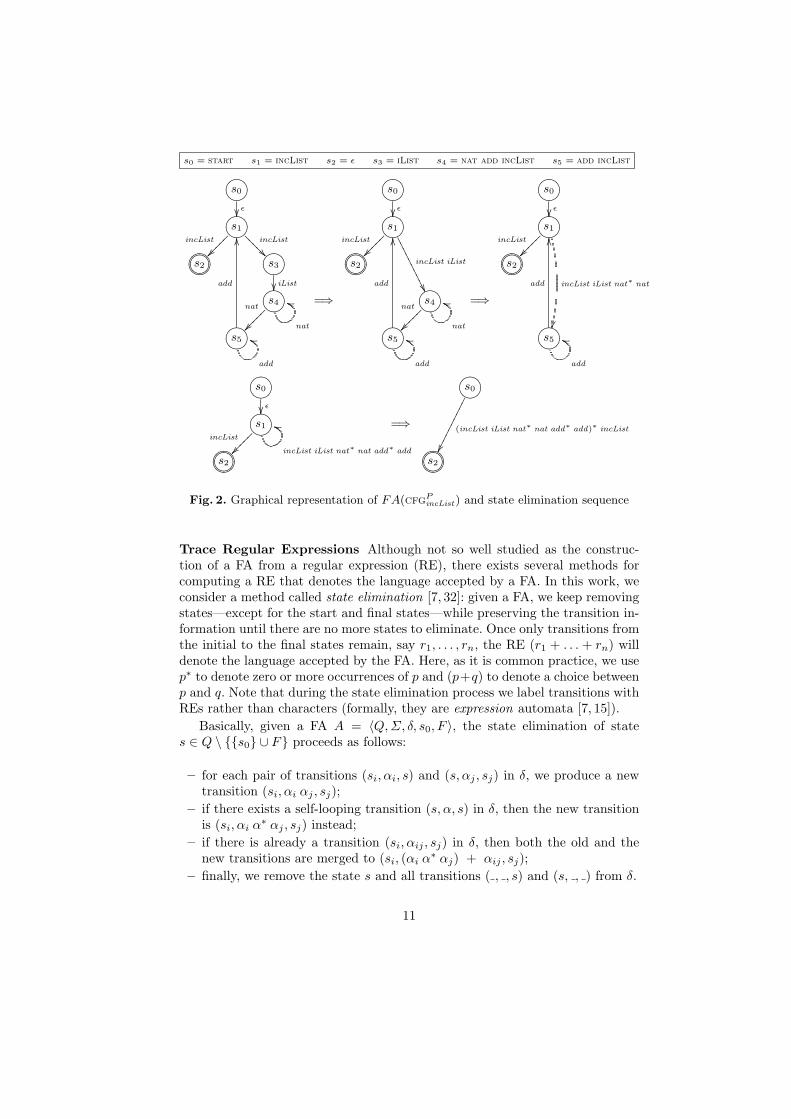
The next example illustrates the construction of a FA from a SRG:

Example 4. Consider the CFG cfgPincList of Example 1 (which, as shown in

Example 2, is already a SRG). The associated FA is

FA(cfgPincList) = 〈Q, incList , iList ,nat , add , ε, δ, s0, s2〉

where

Q = s0, s1, s2, s3, s4, s5δ = (s0, ε, s1), (s1, incList , s2), (s1, incList , s3), (s3, iList , s4),

(s4,nat , s5), (s4,nat , s4), (s5, add , s1), (s5, add , s5)

The FA is graphically shown in the leftmost, topmost corner of Fig. 2, where thefinal state s2 is denoted with a double circle.

10

s0 = start s1 = incList s2 = ε s3 = iList s4 = nat add incList s5 = add incList

?>=<89:;s0

ε?>=<89:;s1

incList

incList

???

??

?>=<89:;76540123s2 ?>=<89:;s3

iList?>=<89:;s4nat

nat

ii =⇒

?>=<89:;s5

add

OO

add

ii

?>=<89:;s0

ε?>=<89:;s1

incList

incList iList

///

////

///

?>=<89:;76540123s2

?>=<89:;s4nat

nat

ii =⇒

?>=<89:;s5

add

OO

add

ii

?>=<89:;s0

ε?>=<89:;s1

incList

incList iList nat∗ nat

?>=<89:;76540123s2

?>=<89:;s5

add

OO

add

ii

?>=<89:;s0

ε?>=<89:;s1

incList

incList iList nat∗ nat add∗ add

ii =⇒

?>=<89:;76540123s2

?>=<89:;s0

(incList iList nat∗ nat add∗ add)∗ incList

?>=<89:;76540123s2

Fig. 2. Graphical representation of FA(cfgPincList) and state elimination sequence

Trace Regular Expressions Although not so well studied as the construc-tion of a FA from a regular expression (RE), there exists several methods forcomputing a RE that denotes the language accepted by a FA. In this work, weconsider a method called state elimination [7, 32]: given a FA, we keep removingstates—except for the start and final states—while preserving the transition in-formation until there are no more states to eliminate. Once only transitions fromthe initial to the final states remain, say r1, . . . , rn, the RE (r1 + . . . + rn) willdenote the language accepted by the FA. Here, as it is common practice, we usep∗ to denote zero or more occurrences of p and (p+q) to denote a choice betweenp and q. Note that during the state elimination process we label transitions withREs rather than characters (formally, they are expression automata [7, 15]).

Basically, given a FA A = 〈Q,Σ, δ, s0, F 〉, the state elimination of states ∈ Q \ s0 ∪ F proceeds as follows:

– for each pair of transitions (si, αi, s) and (s, αj , sj) in δ, we produce a newtransition (si, αi αj , sj);

– if there exists a self-looping transition (s, α, s) in δ, then the new transitionis (si, αi α∗ αj , sj) instead;

– if there is already a transition (si, αij , sj) in δ, then both the old and thenew transitions are merged to (si, (αi α∗ αj) + αij , sj);

– finally, we remove the state s and all transitions ( , , s) and (s, , ) from δ.

11

Different REs can be obtained depending on the order in which states are elim-inated. Clearly, the choice of the next state to be removed is crucial to obtainsimpler REs (see Sect. 4.3 for a particular heuristics).

Example 5. Consider the FA of Example 4, i.e., FA(cfgPincList). The sequence of

state eliminations, using the heuristics of Sect. 4.3, is shown in Fig. 2. Therefore,the associated regular expression is (incList iList nat∗ nat add∗ add)∗ incList .

To summarize, the correctness of our trace analysis, i.e., the fact that the set ofcall sequences in a program belong to the regular language accepted by the gen-erated FA or represented by the associated RE, is a straightforward consequenceof Corollary 1 and results from [24] (for approximating CFGs with SRGs) and[1, 7, 32] (for constructing FAs and REs associated to a SRG).

As for its computational cost, all steps involved in the process are linear inthe size of the source program and, thus, reasonable run times can be expected.

4 Predicting the Effectiveness of Partial Evaluation

The output of the trace analysis gives us the context where every predicate callappears. In this section, we determine (with the help of a termination analysis,namely a size-change analysis) which predicate calls could be deleted by partialevaluation from the computed traces. By analyzing the traces before/after partialevaluation, one can extract useful conclusions on its effectiveness.

4.1 Size-Change Analysis

In this section, we present an informal account of the size-change analysis forlogic programs introduced in [31].

In contrast to other termination analysis for logic programs (e.g., [9, 21]),the size-change analysis of [31] considers strong termination [5], i.e., terminationof all SLD derivations w.r.t. any computation rule. Although this is a strongrequirement, it is quite useful in the context of partial evaluation since it allows usto use rather liberal selection policies at specialization time without recomputingthe termination analysis every time a body atom is marked as “non-unfoldable”(a detailed discussion on this topic can be found in [20]).

Size-change analysis proceeds in two steps: first, size-change graphs are builtwith information on how the size of predicate arguments changes from one callto another; then, a sort of transitive closure is computed in order to identify the(potential) program loops. Size-change graphs are parametric w.r.t. a reductionpair (%,) which is induced from a symbolic norm ||·||:Definition 4 (symbolic norm [21]). Given a term t,

||t|| =

m +∑n

i=1 ki||ti|| if t = f(t1, . . . , tn), n > 0t if t is a variable

where m and k1, . . . , kn are non-negative integer constants depending only onf/n. Note that we associate a variable over integers to each logical variable (weuse the same name for both since the meaning is clear from the context).

12

Then, we have t1 t2 (resp. t1 % t2) if ∀||t1|| > ||t2|| (resp. if ∀||t1|| > ||t2||).Here, the use of variables in the range of symbolic norms provides a simplemechanism to express dependencies between the sizes of terms. Two popularinstances of symbolic norms are the symbolic term-size norm ||·||ts (which countsthe arities of the term symbols) and the symbolic list-length norm ||·||ll (whichcounts the number of elements of a list), e.g.,

f(X, Y ) f(X, a) since ||f(X, Y )||ts = X + Y + 2 > X + 2 = ||f(X, a)||ts[X|R] % [a|R] since ||[X|R]||ll = R + 1 > R + 1 = ||[a|R]||ll

For every pair of atoms (H,Bi) associated to a clause H ← B1, . . . , Bn withn > 0 (i.e., there are no size-change graphs associated with facts), we constructa size-change graph with edges between the arguments of H and Bi when thesize of the corresponding terms decrease w.r.t. a given reduction pair (%,).

Example 6. Consider the program of Example 1. In this case, the size-changegraphs associated to, e.g., clause c3 are as follows:

iList/4 −→ nat/1 iList/4 −→ add/3 iList/4 −→ incList/31iList 1nat

2iList

3iList

% 88pppppppp

4iList

1iList%

..

1add

2iList 2add

3iList

%

??

3add

4iList

88

1iList 1incList

2iList

% 33hhhhhhh2incList

3iList

% 33hhhhhhh3incList

4iList

33hhhhhhh

using a reduction pair induced from the symbolic term-size norm.

Now, in order to identify the program loops, we should compute roughly a tran-sitive closure of the size-change graphs by composing them in all possible forms.Basically, given two size-change graphs:

G = (1p, . . . , np, 1q, . . . ,mq, E1) H = (1q, . . . ,mq, 1r, . . . , lr, E2)

w.r.t. the same reduction pair (%,), their concatenation is defined by

G • H = (1p, . . . , np, 1r, . . . , lr, E)

where E contains an edge from ip to kr iff E1 contains an edge from ip to somejq and E2 contains an edge from jq to kr. Furthermore, if some of the edges arelabeled with , then so is the edge in E; otherwise, it is labeled with %.

Among all computed concatenations of size-change graphs, we only need toconsider the idempotent graphs (i.e., those graphs G with G • G = G), becausethey represent the (potential) program loops.

13

Example 7. For the program of Example 1, we compute the following idempotentsize-change graphs:

incList/3 −→ incList/3 iList/4 −→ iList/4 add/3 −→ add/3

1incList // 1incList

2incList

% // 2incList

3incList // 3incList

1iList 1iList

2iList //

00

2iList

3iList

% // 3iList

4iList // 4iList

1add // 1add

2add

% // 2add

3add // 3add

nat/1 −→ nat/1

1nat // 1nat

These graphs represent how the sizes of the arguments of the three potentiallylooping predicates decrease from one iteration to the next.

In the following, we denote by callsRP (Q0) the set of calls in the computations ofa goal Q0 with program P and a computation rule R. Also, we say that a queryQ is strongly terminating w.r.t. a program P if every SLD derivation for Q withP and R is finite for any computation rule R.

Once the idempotent size-change graphs of a program are computed, thefollowing result characterizes its strong termination. Basically, we require thestrictly decreasing parameters of (potentially) looping predicates to be instanti-ated enough8 w.r.t. a given symbolic norm in the considered computations:

Theorem 2 (strong termination [31]). Let P be a program and (%,) be areduction pair induced by a symbolic norm ||·||. Let A be a set of atoms. If everyidempotent size-change graph for P contains at least one edge ip

−→ ip such that,for every atom A ∈ A, computation rule R, and atom p(t1, . . . , tn) ∈ callsRP (A),ti is instantiated enough w.r.t. ||·||, then P is strongly terminating w.r.t. A.

Note that ti should be instantiated enough in every possible derivation for theconsidered set of atoms w.r.t. any computation rule. Obviously, this is an unde-cidable condition because the set callsRP (A) is generally infinite. Luckily, in thecontext of partial evaluation this condition can be simply approximated by usingthe information provided by a standard binding-time analysis (which is alreadyavailable in many partial evaluators).

Example 8. Consider the program of Example 1 and the idempotent size-changegraphs of Example 7. Here, Theorem 2 guarantees the termination of SLD reso-lution (with any computation rule) for those computations in which the followingparameters are instantiated enough w.r.t. the symbolic term-size norm ||·||ts:

– either the first or the third parameter of incList ,– either the second or the fourth parameter of iList ,– the first parameter of nat , and– either the first or the third parameter of add .

8 A term t is instantiated enough w.r.t. a symbolic norm || · || if ||t|| is an integerconstant [21]. A closely related notion is that of rigidity [6], where a term t is rigidw.r.t. a norm ||·|| if, for any substitution σ, ||tσ|| = ||t||.

14

4.2 Transforming Call Traces

In this section, we consider that the call traces of a program P are safely ap-proximated by a finite automaton FAP constructed as in Sect. 3 (extending theforthcoming transformation to regular expressions is straightforward). We alsoconsider that the output of a binding-time analysis (BTA) is available. This isnot a limitation since current offline partial evaluators for logic programs includea BTA (e.g., Logen [19]).

Here, for simplicity, we consider that the BTA takes a program and an ab-stract atom, i.e., an atom of the form p(b1, . . . , bn) with p/n ∈ Π and bi ∈ s, dfor i = 1, . . . , n, and returns a division that classifies every program parameteras either static or dynamic.9 We denote a division by a set of abstract atoms;furthermore, we consider that divisions contain one (and only one) abstract atomfor each predicate (i.e., we consider a monovariant BTA).

Our first transformation deals with intermediate predicates, i.e., non-recursivepredicates that can be safely unfolded at specialization time. This transforma-tion is related to the transition compression of traditional partial evaluation [18]and is independent of the computed division.

In what follows, given a state s, each transition (s, , s′), s 6= s′, is called anout-transition of s, each transition (s′, , s), s 6= s′, is called an in-transition ofs, and each transition (s, , s) is called a self-looping transition of s.

Definition 5 (elimination of intermediate states).Let FAP = 〈Q,Σ, δ, s0, F 〉 be the trace FA associated to program P . Let s ∈Q \ s0 ∪ F be a state. We say that s ∈ Q is an intermediate state if δcontains exactly one in-transition (s′, q′, s), one out transition (s, q′′, s′′), andno self-looping transition for s. In this case, FAP can be transformed into

FA′P = 〈Q,Σ, δ \ (s, q′′, s′′) ∪ (s, ε, s′′), s0, F 〉

The transformation is applied iteratively as long as FA′P differs from FAP .

As an example, one can consider the FA shown in the leftmost, topmost cornerof Fig. 2. Here, state s3 is an intermediate state and can thus be eliminated.Observe that, in contrast to the state elimination of Sect. 3.3 (which returns thesecond FA in Fig. 2), we do keep the “eliminated” state and just replace theterminal symbol in the out-transition with ε (see Fig. 3 (a)). This will simplifythe comparison between the original and the transformed FAs.

The rationale for our transformation is as follows: the labels of the out-transitions for intermediate states correspond to predicates that are called froma single program point. Therefore, we can safely unfold these calls during spe-cialization and, hence, they will not appear in the partially evaluated program.

Our second, and most important, transformation deals with the output of thesize-change analysis and is parameterized by a given division. Roughly speaking,9 In practice, we would get more accurate results by considering a BTA that com-

putes binding types as in [12], which suffices for checking the “instantiated enough”condition of Theorem 2.

15

?>=<89:;s0

ε?>=<89:;s1

incList

incList

???

??

?>=<89:;76540123s2 ?>=<89:;s3

ε?>=<89:;s4nat

nat

ii

?>=<89:;s5

add

OO

add

ii

(a)

?>=<89:;s0

ε?>=<89:;s1

incList

incList

???

??

?>=<89:;76540123s2 ?>=<89:;s3

ε?>=<89:;s4ε

ε

ii

?>=<89:;s5

ε

OO

ε

ii

(b)

?>=<89:;s0

ε?>=<89:;s1

ε

ε

???

??

?>=<89:;76540123s2 ?>=<89:;s3

ε?>=<89:;s4nat

nat

ii

?>=<89:;s5

add

OO

add

ii

(c)

Fig. 3. Transformation of trace FAs

the information in the division is used to determine which predicate argumentsare statically controlled (i.e., they fulfill the termination condition of Theorem 2).

Definition 6 (elimination of static loops).Let FAP = 〈Q,Σ, δ, s0, F 〉 be the trace FA associated to program P . Let G be theset of idempotent size-change graphs of P and µ a division.

Then, we say that a predicate q ∈ Σ is statically controlled if, for each idem-potent size-change graph G ∈ G for q, there exists at least one edge iq

−→ iqsuch that q(b1, . . . , bi, . . . , bn) ∈ µ and bi = s.10

Now, for each statically controlled predicate q, we transform FAP into FA′P =

〈Q,Σ \ q, δ′, s0, F 〉, where δ′ is obtained from δ by replacing each transition(s, q, s′) with (s, ε, s′).

The rationale for this transformation is as follows: if the condition of Theorem 2hold for a given predicate, all calls to this predicate can be finitely unfolded withthe available information (denoted by a division) and, thus, one can expect thatany reasonable partial evaluator will remove it during specialization.

Example 9. Consider the program of Example 1 and the idempotent size-changegraphs shown in Example 7. The original trace FA for this program is shownin the leftmost, topmost corner of Fig. 2. After the elimination of intermediatestates (the case of s3), we get the trace FA shown in Fig. 3 (a).

Now, if we consider the following division:

µ1 = incList(d, s, d), iList(d, d, s, d), nat(s), add(s, d, d)

10 With a more accurate BTA, this condition could be relaxed to require a parameterwhich is instantiated enough w.r.t. the symbolic norm of the size-change analysis.

16

then nat and add become statically controlled and, hence, we get the transformedtrace FA of Fig. 3 (b). Finally, if we consider the following division:

µ2 = incList(s, d, d), iList(s, s, d, d), nat(d), add(d, s, d)

then incList and iList are now statically controlled and hence we get the trans-formed trace FA of Fig. 3 (c).

Clearly, we could eliminate those states whose transitions are all labeled withε similarly to the standard state elimination process of Sect. 3.3. However, wethink that keeping the structure of the original trace FA may help the user—andautomated analysis tools—to formally compare the original and transformedtrace FAs.

For instance, if we look at the trace FA of Fig. 3 (a), we can conclude thateven if no static information is provided, a significant optimization can still beachieved by partial evaluation: in every iteration for incList an unfolding is saved(the call to iList).

Consider now the trace FA of Fig. 3 (b). Here, we achieve even a moresignificant improvement since, in every iteration for incList , we save not onlythe unfolding of iList but also the complete evaluation of the recursive calls tonat and add .

Finally, consider the trace FA of Fig. 3 (c). Here, we could expect a similar runtime for the specialized program as in the case of Fig. 3 (a) since the eliminationof the outer loop (predicates incList and iList) will only imply saving a constantnumber of steps (that are moved from run time to partial evaluation time).

4.3 The Approach in Practice

A prototype tool, called Pepe, for estimating the speedup of partial evaluationhas been developed. It is implemented in Prolog and includes the trace analysisof Sect. 3, the size-change analysis of Sect. 4.1, and a simple (monovariant) BTA.

Given a program and an abstract atom, the tool returns two regular ex-pressions that represent the call traces of the original and partially evaluatedprograms. The tool is publicly available through a simple web interface fromhttp://german.dsic.upv.es/pepe.html. This is mainly a proof-of-concept im-plementation and much work can still be done to improve it, e.g., depictinggraphically the finite automata rather than their associated textual regular ex-pressions, allowing the user to focus on how a given part of the program wouldchange by the partial evaluation, adding automated tools for determining thebest division (or the best one from a number of alternatives), etc.

Actually, a challenge of the current implementation is showing the shortestpossible regular expression. A drawback of the state elimination method is thatdifferent sequences of state removals may give rise to different regular expressionsfor the same language. There exists in the literature several approaches that allowone to produce shorter regular expressions, e.g., [13, 16]. In particular, we haveimplemented a slight variant of the technique in [13], which proposes a heuristicsbased on assigning weights to the states of the FA and then choosing the state

17

Table 1. Experimental results

Benchmark Trace Regular Expressions (original/specialized)

applast(d, s, d) applast app* app (last last_)* last

run time speedup: 2.5 _______ app* app (last _____)* last

incList(s, d, d) (incList iList nat* nat add* add)* incList

run time speedup: 0.98 (_______ _____ nat* nat add* add)* _______

incList(d, s, d) (incList iList nat* nat add* add)* incList

run time speedup: 5.25 (incList _____ ___* ___ ___* ___)* incList

match(s, d) match (loop eq)* loop + match (loop eq + loop neq next)* loop

run time speedup: 6.72 _____ (loop __)* loop + _____ (loop __ + loop ___ next)* loop

power(d, s, d) power* power (mult* mult (add* add)*)*

run time speedup: 1.21 _____* _____ (mult* mult (add* add)*)*

with the lightest weight. Given a transition (s, α, s′), its weight is the number ofcharacters in α. Then, the weight of a state is obtained as the sum of the weightsof its in-transitions, its out-transitions, and its self-looping transitions.

Consider, e.g., the FA in the leftmost, topmost corner of Fig. 2. Then, theweight of the states—which are not a start or a final state—is as follows:11

s1 = 3 s3 = 2 s4 = 3 s5 = 3

Thus the first state to be removed is s3. In the next FA of the sequence, we havethe following weights:

s1 = 4 s4 = 4 s5 = 3

Therefore, either s1 or s4 could be removed. Here, we consider first those stateswith exactly one in-transition and one out-transition (this is a refinement overthe standard technique of [13] that gives good results in our setting). Hence states4 is chosen. The new weights are as follows:

s1 = 6 s5 = 6

Again, both states have the same weight, but only s5 fulfill the above condition.Thus we first remove s5 and, finally, s1.

Now, we show the results of a preliminary experimental evaluation with sometypical benchmarks. Table 1 shows, for each benchmark, the abstract atom usedfor the partial evaluation, the experimental speedup (obtained by partially eval-uating them with Proff [28], a simple offline partial evaluator for pure Prolog),the original regular expression and the transformed one according to Sect. 4.2.

Observe, for instance, the case of incList (the program of Example 1):having a static first argument, as in incList(s, d, d), has no (positive) impacton the associated partial evaluation since no call in the main loop is removed;in contrast, it is the main loop that is fully unrolled. Here, the slight slowdowncould be explained by the likely increase in code size and memory consumption11 Note that every predicate symbol is considered as a single character.

18

due to loop unrolling. In contrast, if we consider incList(d, s, d), the outer loopfor incList remains but all calls to iList, nat, and add are fully unfolded,which explains the significant performance improvement. Benchmarks applastand match are classical examples where partial evaluation may get a significantimprovement. As can be seen in the associated regular expressions, some stepsinside a loop are reduced in each example. Finally, benchmark power showsan example where only some calls to power are unfolded (hence a constantimprovement) and, thus, no significant speedup is achieved.

Clearly, the finite automata or regular expressions produced by our techniqueare not always easy to analyze. For small examples, they can help the user tounderstand why adding more static information has no effects in some cases, whysignificant improvements can be achieved even with no static data, etc. For largerprograms, however, the analysis becomes rather complex and the developmentof analysis techniques and tools will be required, an interesting topic for furtherresearch.

5 Related Work

We find very few works devoted to formally analyze the effectiveness of partialevaluation. For instance, [3] establishes several properties of program transfor-mations based on folding/unfolding in the context of logic programming. Inparticular, he proves that superlinear speedup cannot be accomplished by par-tial evaluation (this result can also be found in [4] for a flow chart language).[4] develops a speedup analysis that, for any binding-time annotated program,computes a relative speedup interval such that the specialization of this programwill result in a speedup within the predicted interval. Our approach is partly in-spired by the work of [4], but several significant differences exist: they determinethe program loops statically in the source program, while we use a combinationof size-change analysis and trace analysis to identify the program loops and thecontext where they appear; [4] is formalized in the context of a simple flow chartlanguage, while we consider a logic programming language; they do not distin-guish whether the static parameters decrease strictly or non-strictly from onecall to another, while this is essential in our approach.

Regarding our trace analysis, we share the aims of previous work by Gallagherand Lafave [14]. There are, however, a number of important differences: they gen-erate trace terms abstracting computation trees independently of a computationrule, while we generate sequences of predicate calls for a specific computationrule; also, their approximation technique is based on abstract interpretation [10],while ours is based on (simpler) techniques from formal languages and automatatheory; the main difference, though, is that they do not include a technique forenumerating the (possibly infinite) set of trace terms of a program, while thisis a key ingredient of our approach, where call traces are elegantly representedby means of finite automata or regular expressions (since they form a regularlanguage, in contrast to the trace terms of [14]).

19

As mentioned in Sect. 1, there are some recent approaches (e.g., [11, 27])where experimental frameworks for estimating the best division are introduced.Although their aim is similar to ours, we put the emphasis on developing asymbolic framework and thus our goals are different. Indeed, both approachescan be seen as complementary.

To summarize, this work constitutes our last contribution from a long-termresearch on formally measuring and estimating the effects of partial evalua-tion (see, [2, 29, 30]). These works, however, never considered prediction (i.e.,speedups were measured a posteriori).

6 Conclusions and Future Work

Predicting the potential speedup that can be achieved by partial evaluation isa challenge that has received little attention so far. In this work, we introduceda symbolic framework for analyzing the effects of a partial evaluation given aprogram and an initial call. Basically, we use a size-change analysis to determinewhich recursive predicates could be safely unfolded because their control flow isstatically determined by the available information. Then, a trace analysis hasbeen introduced in order to get the context of each procedure call, so that theimpact of its elimination can be better estimated.

The techniques introduced in this paper can be seen as a first step for thedevelopment of automated quantitative techniques and tools for predicting thepotential speedup, thus it opens a number of interesting lines for further research.For instance, we could define formal techniques for comparing finite automataor regular expressions (with the same structure), simple cost models based onthe output of the trace analysis, tools for easing the graphical inspection of largefinite automata and regular expressions, etc.

Acknowledgments

We would like to thank Elvira Albert, Sergio Antoy, Manuel Hermenegildo,Michael Leuschel, Claudio Ochoa, and German Puebla for many interesting dis-cussions on the topic of this paper.

References

1. A.V. Aho and J.D. Ullman. The Theory of Parsing, Translation and Compiling.Prentice-Hall, 1973.

2. E. Albert, S. Antoy, and G. Vidal. Measuring the Effectiveness of Partial Eval-uation in Functional Logic Languages. In Proc. of the 10th Int’l Workshop onLogic-based Program Synthesis and Transformation (LOPSTR’00), pages 103–124.Springer LNCS 2042, 2001.

3. T. Amtoft. Properties of Unfolding-based Meta-level Systems. In Proc. of theACM Symp. on Partial Evaluation and Semantics-based Program Transformation(PEPM’91), 1991.

20

4. L.O. Andersen and C.K. Gomard. Speedup Analysis in Partial Evaluation: Pre-liminary Results. In Proc. of the ACM Workshop on Partial Evaluation andSemantics-based Program Transformation (PEPM’92), pages 1–7. Yale University,New Haven, CT, 1992.

5. M. Bezem. Strong Termination of Logic Programs. Journal of Logic Programming,15(1&2):79–97, 1993.

6. A. Bossi, N. Cocco, and M. Fabris. Proving Termination of Logic Programs byExploiting Term Properties. In S. Abramsky and T.S.E. Maibaum, editors, Proc.of TAPSOFT’91, pages 153–180. Springer LNCS 494, 1991.

7. J.A. Brzozowski and E.J. McCluskey. Signal Flow Graph Techniques for SequentialCircuit Diagrams. IEEE Trans. on Electronic Computers, EC-13:67–76, 1963.

8. N. Chomsky. On certain formal properties of grammars. Information and Control,2:137–167, 1959.

9. M. Codish and C. Taboch. A Semantic Basis for the Termination Analysis of LogicPrograms. Journal of Logic Programming, 41(1):103–123, 1999.

10. P. Cousot and R. Cousot. Abstract Interpretation: A Unified Lattice Model forStatic Analysis of Programs by Construction or Approximation of Fixpoints. InProc. of Fourth ACM Symp. on Principles of Programming Languages, pages 238–252, 1977.

11. S. Craig and M. Leuschel. Self-Tuning Resource Aware Specialisation for Prolog.In Proc. of PPDP’05, pages 23–34. ACM Press, 2005.

12. S.-J. Craig, J. Gallagher, M. Leuschel, and K.S. Henriksen. Fully Automatic Bind-ing Time Analysis for Prolog. In Proc. of the Int’l Symposium on Logic-based Pro-gram Synthesis and Transformation (LOPSTR’04), pages 53–68. Springer LNCS3573, 2005.

13. M. Delgado and J. Morais. Approximation to the Smallest Regular Expression fora Given Regular Language. In Proc. of the 9th Int’l Conf. on Implementation andApplication of Automata (CIAA’04), pages 312–314. Springer LNCS 3317, 2004.

14. J.P. Gallagher and L. Lafave. Regular Approximation of Computation Paths inLogic and Functional Languages. In Partial Evaluation, International Seminar,Dagstuhl Castle, Germany, February 12-16, 1996, Selected Papers, pages 115–136.Springer LNCS 1110, 1996.

15. Y.-S. Han and D. Wood. The generalization of generalized automata: Expressionautomata. International Journal of Foundations of Computer Science, 16:499–510,2005.

16. Y.-S. Han and D. Wood. Obtaining shorter regular expressions from finite-stateautomata. Theoretical Computer Science, 370(1-3):110–120, 2007.

17. J.E. Hopcroft and J.D. Ullman. Introduction to Automata Theory, Languages andComputation. Addison-Wesley, 1979.

18. N.D. Jones, C.K. Gomard, and P. Sestoft. Partial Evaluation and Automatic Pro-gram Generation. Prentice-Hall, Englewood Cliffs, NJ, 1993.

19. M. Leuschel, J. Jørgensen, W. Vanhoof, and M. Bruynooghe. Offline Specialisationin Prolog using a Hand-Written Compiler Generator. Theory and Practice of LogicProgramming, 4(1-2):139–191, 2004.

20. M. Leuschel and G. Vidal. Fast Offline Partial Evaluation of Large Logic Programs.In Proc. of the 18th Int’l Symposium on Logic-based Program Synthesis and Trans-formation (LOPSTR 2008). Technical University of Valencia, 2008. Available fromhttp://www.dsic.upv.es/~gvidal/german/papers.html. To appear.

21. N. Lindenstrauss and Y. Sagiv. Automatic Termination Analysis of Logic Pro-grams. In Proc. of Int’l Conf. on Logic Programming (ICLP’97), pages 63–77. TheMIT Press, 1997.

21

22. J.W. Lloyd. Foundations of Logic Programming. Springer-Verlag, Berlin, 1987.Second edition.

23. J.W. Lloyd and J.C. Shepherdson. Partial Evaluation in Logic Programming.Journal of Logic Programming, 11:217–242, 1991.

24. M. Mohri and M.-J. Nederhof. Regular Approximation of Context-Free Grammarsthrough Transformation, chapter 9, pages 153–163. Kluwer Academic Publishers,The Netherlands, 2001.

25. M. Mohri and F.C.N. Pereira. Dynamic Compilation of Weighted Context-FreeGrammars. In Proc. of the 36th Annual Meeting of the Association for Computa-tional Linguistics and the 17th Int’l Conf. on Computational Linguistics (COLING-ACL’98), pages 891–897, 1998.

26. M.-J. Nederhof. Regular approximation of CFLs: a grammatical view, chapter 12,pages 221–241. Kluwer Academic Publishers, The Netherlands, 2000.

27. C. Ochoa and G. Puebla. Poly-controlled Partial Evaluation in Practice. In Proc.of the 2007 ACM SIGPLAN Workshop on Partial Evaluation and Semantics-basedProgram Manipulation (PEPM’07), pages 164–173. ACM, 2007.

28. S. Tamarit and G. Vidal. PROFF - A PRolog OFFline partial evaluator. URL:http://german.dsic.upv.es/proff.html, 2007.

29. G. Vidal. Cost-Augmented Narrowing-Driven Specialization. In Proc. of the ACMSIGPLAN Workshop on Partial Evaluation and Semantics-Based Program Manip-ulation (PEPM’02), pages 52–62. ACM Press, 2002.

30. G. Vidal. Cost-Augmented Partial Evaluation of Functional Logic Programs.Higher-Order and Symbolic Computation, 17(1-2):7–46, 2004.

31. G. Vidal. Quasi-Terminating Logic Programs for Ensuring the Termination ofPartial Evaluation. In Proc. of the ACM SIGPLAN 2007 Workshop on PartialEvaluation and Program Manipulation (PEPM’07), pages 51–60. ACM Press, 2007.

32. D. Wood. Theory of Computation. John Wiley & Sons, Inc., New York, NY, 1987.

22