Effectiveness of Recent Fiber-interaction Diffusion Models for

Orientation and the Part Stiffness Predictions in Injection Molded

Short-fiber Reinforced Composites

Babatunde O. Agboolaa, David A. Jackb, S. Montgomery-Smithc

aDepartment of Mechanical Engineering, Baylor University, Waco, TX 76798, U.S.A.bDepartment of Mechanical Engineering, Baylor University, Waco, TX 76798, U.S.A.cDepartment of Mathematics, University of Missouri, Columbia MO 65211, U.S.A.

Abstract

Two fiber interaction models for predicting the fiber orientation and resulting stiffness of a

short-fiber reinforced thermoplastic composite are investigated, the isotropic rotary diffusion

of Folgar and Tucker (1984) and the anisotropic rotary diffusion of Phelps and Tucker (2009).

This study employs several fiber orientation tensor closure approximations for both diffusion

models and results are compared to those from the numerically exact spherical harmonic

approach. Results are presented for variations in the fiber orientation and the processed

part stiffness. A significant difference was observed between the stiffness predicted by both

rotary diffusion models. It is worth noting that not all closures behave the same between

the diffusion models, thus encouraging further studies to refine and validate the new fiber

interaction models and solution approaches. A study of the predicted flexural modulus is

presented, and results suggest that flexural modulus experiments may aid in further refining

the fiber interaction models.

Keywords: B. Directional Orientation B. Mechanical Properties C. Computational

Modeling E. Injection molding

1. Introduction and overview of problem

Short-fiber reinforced thermoplastic composites have received widespread use due to the

enhancement of the structural properties of a polymer component at a minimal cost. The

fibers are suspended within the polymer matrix during processing and orient in response to

the flow kinematics of the polymer melt. The motion and orientation of fibers is influenced

Preprint submitted to Composites, Part A May 15, 2012

by the kinematics of the flow and by interactions with adjacent fibers. Thus the orientation

of short-fibers in an injection molded composite will vary within the part, producing spatial

inhomogeneity in the orientation and anisotropy of the mechanical properties. Accurate

and efficient predictions of the orientation and the resulting material properties will be very

useful for controlling and designing injection molding manufacturing processes to obtain

suitable parts. Consequently, many researchers have developed models that accurately and

efficiently predict the flow induced orientation of short fibers within a thermoplastic (see

e.g., [1, 2, 3, 4, 5, 6]).

The Jeffery model [7] forms the basis for most models that predict the fiber orientation

evolution within a composite and is valid for a single fiber in a thermoplastic melt of a dilute

suspension. A thermoplastic is a non-Newtonian fluid, but over the length scale of the fiber

the velocity gradients are effectively constant. Therefore a single shear is experienced by the

entire fiber thus not violating the Jeffery assumption of a locally Newtonian fluid. Due to the

overwhelming computational burden in quantifying the motion of every fiber within the melt,

an orientation probability distribution function (ODF) is used to describe the orientation

of collections of fibers (see e.g., [2, 8]). The ODF is a complete, unambiguous description

of the fiber orientation state and can be calculated from the processing conditions. Typical

approaches to solve the equation of motion of the ODF rely on the control volume approach

(see e.g., Bay [3]) which take days to solve for simple flows (see e.g., [3, 9, 10, 11]). The control

volume solution approach of Bay [3] has been considered to yield the most accurate solutions

of the ODF. Recently, Montgomery-Smith et al. [12] introduced the computationally efficient

spherical harmonic approach which yields identical results to those of the Bay approach, but

reduces the computational time from days to minutes for the same flows. In principle the

spherical harmonic approach can be incorporated within a finite element software package

for cavity simulations of the flow, but the scope of the memory requirements along each

streamline of the flow currently make it impractical for industrial use.

Advani and Tucker [2, 8], cast the evolution equation of the ODF in terms of the moments

of the orientation distribution [2], and called the resulting form of these moments the ori-

entation tensors. Solutions of the orientation tensor equation of motion for the flows along

an individual streamline can be solved in a matter of seconds [11] and are concise enough to

2

be utilized in industrial finite element codes. The orientation tensor approach suffers from

the need for a higher order tensor to solve the equation of change. This brings about the

need for a closure approximation of a higher order tensor in terms of a lower order tensor [2].

Researchers have proposed various forms for closure approximations [8, 4, 13, 14, 15, 4, 16],

where the effectiveness of each model has been demonstrated only on the particular fiber

interaction model for which they were developed. Montgomery-Smith et al. [17, 18] recently

proposed a new closure called the fast exact closure (FEC), which combines the efficiency

of the commonly used hybrid closure [2] and the accuracy of the ORT closure [19]. In the

present paper, all results will be compared to the spherical harmonic solutions obtained

using the method in [12]. This approach was demonstrated to retain the full accuracy of

the ODF solution and is only limited by the numerical precision of the computer. Thus the

spherical harmonic solution is considered true, if one assumes the diffusion model itself from

the governing equation is true. Thus one can objectively compare the spherical harmonic

solutions between two fiber interaction models without any bias from the choice of closure.

For concentrated suspensions, a rotary diffusivity term Dr is added to Jeffery’s form of the

ODF to account for the interaction of fibers. Folgar and Tucker [1] suggested that Dr relates

to a statistical parameter called the interaction coefficient CI . This empirical parameter

has values that increase with the concentration of the fiber-plastic suspension as well as the

fiber aspect ratio. The Folgar-Tucker model is independent of direction and throughout the

text will be called the isotropic rotary diffusion (IRD) model. The IRD model tends to

over predict the orientation kinetics of the fibers (see e.g., [6]), but is widely available in

commercial software packages used for the design of injection molds. To solve this problem

of the alignment rate, researchers have tried to find ways to slow down the orientation

kinetics using physically meaningful approaches. Wang et al. [20] recently proposed an

objective diffusion model to slow the orientation kinetics, called the reduced strain closure

(RSC) model. Phelps and Tucker [6] further improved on the RSC model by introducing

a directional dependance to the fiber interactions through the diffusion term of the ODF

equation of motion and compared their results to experimental observations.

It has been noted that the fiber orientation kinematics are coupled with the flow kinetics

for densely packed flows (see e.g., [21, 22]), and several researchers have provided solutions

3

using the full coupled form of orientation and flow (see e.g., [19, 23, 24]). It has been

demonstrated in Wang et al. [20] that the incorporation of the full fiber orientation/flow

velocity coupling is insufficient in predicting the fiber orientation correctly, where the greater

impact is the choice of diffusion model. In the present context, so as not to obfuscate the

comparisons between fiber interaction models, we will neglect coupling to bring attention

to the two classes of diffusion models themselves. Full simulations of industrial injection

molded composites will need to include the full coupling as well as selecting the proper fiber

interaction model. The interested reader is encouraged to read Verweyst and Tucker [19]

and Chung and Kwon [23] for extensive studies of the impact the full coupling has on the

processed part stiffness when one uses the IRD fiber interaction model.

Advani and Tucker [8] linked the stiffness of the solidified part to the underlying orien-

tation microstructure using an orientation averaging approach. Jack and Smith [25] derived

the stiffness expectation from the fourth-order orientation tensor along with the variance

of the stiffness, which is a function of the eighth-order orientation tensor. The relationship

between the orientation tensor and the resulting stiffness was validated by Caselman [26]

and was used by Gusev et al. [27, 28]. Recently, Nguyen et al. [29] used the anisotropic

rotary diffusion (ARD) model by Phelps and Tucker [6] with the ORT closure to predict the

stress/strain response for injection molded long fiber thermoplastics. Although their results

are quite impressive, it is unclear to what extent the closure choice may bias the solution.

The objectives of this paper are, (1) to compare the IRD and the ARD diffusion models

using the numerically exact spherical harmonic approach, (2) investigate the impact the

choice of diffusion model has on the resulting stiffness, the natural frequency, and the flexural

modulus of the processed composite, and (3) to investigate if the preferred closure for solving

the orientation kinetics may be different between the two diffusion models.

2. Fiber Orientation Modeling

The study of the motion of short fibers in a fluid is often based on the motion of an

individual particle using Jeffery’s model [7] which captures the motion of rigid ellipsoidal

particles through the equation of change for the unit direction vector p along the major

axis. For typical industrial use, the modeling of individual fibers is computationally imprac-

4

tical, instead the fiber orientation distribution function ψ (p), which will be call the ODF

throughout the text, is used to describe the fiber orientation. The motion of a fiber within a

concentrated suspension will be impeded by the motion of the neighboring fibers. This has

lead to the development of interaction parameters often lumped into a rotary diffusion term

Dr of the constitutive equation popularized by Bird et al. [30] (sometimes referred to as the

generalized Fokker-Planck or the Smoluchowski equation) as

Dψ

Dt= −1

2∇p · (Ω · p+ λ (Γ · p− λΓ : ppp)ψ) +∇p · ∇p(Drψ) (1)

where the fiber is assumed to move with the the bulk motion of the fluid, and ψ is regarded

as a convected quantity. In Equation (1), ∇p is the gradient operator on the surface of a

unit sphere (i.e., the gradient operator in orientation space), p is the material derivative

of p defined as DpDt

= ∂p∂t

+ v · ∇. The tensor Γ = ∇v + ∇vT is the rate of deformation

of the surrounding fluid, Ω = ∇v − ∇vT is the vorticity tensor of the fluid, v is the fluid

velocity, and λ is a function of the equivalent ellipsoidal fiber aspect ratio ae (see e.g., [31]

on computing ae for cylindrical and various other shaped fibers). The isotropic and an

anisotropic form of the rotary diffusion term Dr will be discussed later in this text.

The spherical harmonic expansion of ψ(θ, ϕ) proposed by Montgomery-Smith et al. [12]

yields a numerically exact systematic approach for solving the ODF of Equation (1). This

approach expands the orientation distribution function, ψ(p), using the complex spherical

harmonics Y ml to any desired order as

ψ(p) =∞∑l=0

l∑m=−l

ψml (p)Y ml (2)

where Y ml are the complex spherical harmonic coefficients and ψml contain information per-

taining to the orientation. The equation of motion for ψ(p) is expanded using Equation

(2) and numerically exact transient solutions, limited only by machine precision, of DψDt

may

be obtained using the spherical harmonic expansion. This new algorithm is exceptionally

efficient as compared to solutions using the control volume method presented by Bay [3],

where the control volume approach requires 2-3 orders of magnitude more time than the

numerically exact spherical harmonic approach.

5

The form of the spherical harmonic solution could be implemented into commercial finite

element solutions of the ODF that may vary in both space and time, but the number of

degrees of freedom at each node make it impractical. Most industrial simulations use the

orientation tensor approach popularized by Advani and Tucker [2], where the second- and

the fourth-order orientation tensor components are defined as

A =

∮S

pp ψ(p) dp

A =

∮S

pppp ψ(p) dp (3)

where∮S(...) dp represents the integral on the unit sphere encompassing all possible fiber

orientations, pipj is the tensor (or dyadic) product of the fiber orientation vector p with itself.

Orientation tensors are completely symmetric, i.e. Aij = Aji and Aijkl = Ajikl = Aklij = . . ..

2.1. Isotropic rotary diffusion (IRD)

The Folgar-Tucker isotropic rotary diffusion (IRD) fiber interaction model is based on the

assumption that all fibers in a melt interact with adjacent fibers in the same way, regardless

of the direction a fiber is pointing. They define Dr from Equation (1) as CIG, where CI

is called the interaction coefficient empirically determined by comparing experimental data

and numerical predictions, and G is the scalar magnitude of the rate of deformation tensor

defined as G =√

12Γ : Γ. The results obtained using the IRD model predict steady fiber

alignment states consistent with experimental observations [6] where the equation of motion

for A may be expressed as (see e.g., [2])

DA

Dt= −1

2(Ω ·A−A ·Ω) +

1

2λ(Γ ·A+A · Γ− 2Γ : A) + 2CIG(I− 3A) (4)

Observe in Equation (4), A appears in the equation of motion for A. Similarly, the motion

equation motion for A has the sixth-order orientation tensor (see e.g., [9]). The orientation

tensor equation of motion for an even ordered tensor will contain the next higher even-

ordered orientation tensor (see e.g., [32]). Therefore, to solve Equation (4) a closure will be

required where A is approximated as a function of A.

2.2. Anisotropic rotary diffusion (ARD-RSC)

Development of anisotropic rotary diffusion (ARD) models has been motivated by at-

tempts to improve on the IRD model, which over predicts the fiber alignment rate observed6

experimentally. Unlike the IRD, the ARD models take into account the directional depen-

dence of fiber-fiber interactions, and there exist several ARD models in the literature (see

e.g., Koch [5], Jack [32], Fan et al. [33], Phan-Thien et al. [34], and Wang et al. [20]).

The most recent ARD model of Phelps and Tucker [6] sought to improve upon the Reduced

Strain Closure (RSC) diffusion model of Wang et al. [20], and the Phelps and Tucker ARD-

RSC model was shown to be in reasonable agreement with experimental observations. The

Phelps and Tucker ARD-RSC equation of motion for A can be expressed as [6]

DA

Dt=

1

2(Ω ·A−A ·Ω) +

1

2λ Γ ·A+A ·Γ− 2 [A+(1−κ) (L−M : A)] :Γ

+γ2[C−(1−κ)M :C]− 2κ(trC)A−5(C ·A+A ·C)+10[A+(1−κ) (L−M :A)] : C (5)

where the second order tensor C is defined in terms of the empirical coefficients bi as

C = b1γI+ b2γA+ b3γA2 +

b42Γ+

b54γ

Γ2 (6)

Note that the values of 12and 1

4that occur in Equation (6) differ from those given in Phelps

and Tucker [6] in that they use 12Γ to define the rate of deformation tensor. An alternative

form is presented in [12], both for the equation of motion for A and for the equation of

motion of ψ (p) that can be numerically solved using spherical harmonics. For simple shear

flow the coefficients bi in Equation (6) were fit in [6] to the experimental observations from

a plaque flow as

b =[1.924× 10−4, 5.839× 10−3, 4.0× 10−2, 1, 168× 10−5, 0

](7)

It is important to emphasize that these parameters will work for the identical flow conditions

in which they were fit (i.e., fiber packing density, flow viscosity, fiber aspect ratio, etc.), but

for general implementations an exhaustive study must be performed to quantify the link

between the coefficients bi and any industrial implementation.

In Equation (5) the parameter κ will vary based on the degree of reduction of the orien-

tation alignment rate desired, and we use the value of κ = 1/30 suggested by Phelps and

Tucker [6]. The two fourth-order tensors M and L in Equation (5) are functions of the

eigenvalues A(i) and eigenvectors ni of A as

M =3∑i=1

nininini, and L =3∑i=1

A(i)nininini (8)

7

2.3. Closure Approximations

The equation of motion for the second-order orientation tensor for both diffusion models,

e.g., Equations (4) and (5), contains the next higher even order orientation tensor. This

brings about the need for a closure approximation to obtain a closed set of equations which

may be generalized in component form as

Aijkl ≈ Fijkl(A) (9)

where Fijkl is a fourth-order tensor function operating on the second-order orientation tensor

A. An objective closure will be independent of the choice of coordinate frame [4]. Based

on the symmetric nature of the orientation tensors defined in Equation (3), a fourth-order

orientation tensor will have at most 15 independent components (which is further reduced

to 14 due to the fact that Aiijj = Aii = 1, sum on i and j).

2.3.1. Hybrid Closure

The hybrid closure [2] is a popular closure in part due to its algebraic simplicity and com-

putational efficiencies, despite some well known drawbacks in over predicting the alignment

state [35]. It is formed from a linear combination of the quadratic closure of Doi [13] and

the linear closure of Hand [14] as

Aijkl = (1− f)Aijkl + fAijkl (10)

where Aijkl is the linear closure and Aijkl is the quadratic closure.

2.3.2. Orthotropic Closure (ORT)

The orthotropic closure approximations have significantly improved on the accuracy of

the hybrid closure, but often at the cost of an increase in computational efforts (see e.g.,

[4, 36, 37, 38]). The orthotropic closures, first proposed by Cintra and Tucker [4], construct

fitted forms of Equation (9) that rely on the invariants or the eigenvalues of the second-order

orientation tensor. The construction of the orthotropic closures constrain the principal axis

of the fourth-order orientation tensor to align with those of the second-order orientation

tensor. The orthotropic closures typically provide the most accurate results when compared

8

to experimentally measured fourth-order orientation tensors [39]. The ORT closure used by

VerWeyst and Tucker [19] is given as

Aclosuremm = C1

m + C2mA(1) + C3

m[A(1)]2 + C4

mA(2) + C5m[A(1)]

2 + C6mA(1)A(2) (11)

where Cim are found by fitting the orientation tensor components from results obtained by

full numerical solution of DψDt

, and A(1) ≥ A(2) ≥ A(3) ≥ 0 with A(1) + A(2) + A(3) = 1.

2.3.3. Neural Network Based Closure

The original Neural Network Based Closure (NNET) by Jack et al. [16] is based on

the artificial neutral network (ANN) fitting technique which mimics the biological signal

processing scheme. The Neural Network Orthotropic Closure (NNORT) closure [10] improves

on the NNET in that it is truly objective and coordinate frame invariant. It combines the

architecture of the ANN and maintains the principles of the orthotropic closures. Both the

NNET and the NNORT are based on a network where the output is computed as

A4 = f2(w2 · f1(w1 · A2 + b1) + b2) (12)

where A4 and A2 are, respectively, the independent values of A and A, w1 and w2 are

the network weights, b1 and b2 are the network biases, and f1 and f2 are, respectively, the

hyperbolic tangent transfer function and the pure linear transfer function. The dimensions

of each of the parameters in Equation (12) differ between the NNET and the NNORT, where

the weights and the biases are obtained through a training algorithm of architecture based

on known inputs and outputs obtained by full solutions of Equation (1) for the IRD fiber

interaction model.

2.3.4. Fast Exact Closure (FEC)

The Fast Exact Closure (FEC) [18, 17] is not a closure approximation in the traditional

sense as it does not rely on an approximation for A, but it will yield exact solutions of

the fiber orientation state in the absence of diffusion. The FEC has computational speeds

comparable to that of the hybrid closure for a variety of diffusion models. The FEC does

not rely on any curve fitting techniques, nor does it rely directly on an elliptic integral

computation. The approach bypasses the fitting process of the orthotropic and the neural9

network closures, and thus may be constructed independent of the diffusion model selected

for the fiber interaction form used in many of the fitting methods. The FEC is generated by

simultaneously solving the ODE’s for two symmetric second-order tensors A and B, where

A is the second-order orientation tensor as defined in Equation (3). The FEC solution for

the IRD fiber interaction model is expressed as

DA

Dt=

1

2C : [B · (Ω+ λΓ) + (−Ω+ λΓ) ·B] +Dr(2I− 6A)

DB

Dt= −1

2(B · (Ω+ λΓ) + (−Ω+ λΓ) ·B)−DrD : (2I− 6A)

(13)

Notice in Equation (13) that there is no need for the classical closure as depicted in Equation

(9) as there is no A appearing in either of the equations of motion. Alternatively there are

two fourth-order conversion tensors C and D. The two tensors convert between DADt

and DBDt

using DADt

= −C : DBDt

and DBDt

= −D : DADt

(see e.g., [18]). The tensor C can be obtained

directly from the eigenvalues of A and B (see e.g [18, 17]) and D is the rank-four tensor that

is the tensor inverse of C. The form of the equations of motion for the ARD-RSC, along with

several alternative anisotropic diffusion forms, is given in Montgomery-Smith et al. [18, 17].

2.4. Material Properties Predictions

Injection molded composites consist of misaligned fibers and using homogenization, the

composite stiffness can be expressed as a function of the fiber orientation and the under-

lying unidirectional stiffness tensor [2, 25]. For unidirectional composites with discontin-

uous reinforcements, Gusev et al. [40, 28] and Tucker and Liang [41] demonstrated that

the Tandon-Weng model [42] yields reasonable predictions of the stiffness and will be used

within the present paper. From this unidirectional stiffness tensor we use the orientation

averaging approach suggested by Advani and Tucker [2] to predict the stiffness variation due

to randomness in the fiber orientation within the composite. The orientation averaging form

of an injection molded short fiber reinforced composite stiffness tensor is given as [2, 25]

⟨Cijkl⟩ = β1(Aijkl) + β2(Aijδkl + Aklδij) + β3(Aikδjl + Ailδjk+

Ajlδik + Ajkδil) + β4(δijδkl) + β5(δikδjl + δilδjk)(14)

10

where the β′is are scalars related to the underlying unidirectional stiffness tensor as

β1 = C1111 + C2222 − 2C1122 − 4C1212

β2 = C1122 + C2222

β3 = C1212 +1

2(C2233 − C2222)

β4 = C2233

β5 =1

2(C2222 − C2233) (15)

Once the stiffness is known, the material stiffness constants are readily extracted (see e.g.,

Jones [43]), such as Eii (i = 1, 2, 3 and no sum on i), Gij (i, j = 1, 2, 3 and i = j), and νij

(i, j = 1, 2, 3 and i = j), which are, respectively, the Young’s modulus along the xi axis, the

Shear modulus in the xi−xj plane and the Poisson’s Ratio on the xi face in the xj direction.

Notice in Equation (14) the appearance of Aijkl as well as Aij. When solving the equa-

tion of motion for the second-order orientation tensor, which already requires the use of a

closure to approximate Aijkl, it is customary to use the same closure in the material stiffness

calculation to compute Cijkl of the fully hardened composites, but this is by no means a

requirement. For the orientation evolution of Aij from the FEC closure, in Equation (13),

notice only A and B appear, both second order tensors and nowhere is A directly computed.

As discussed in Montgomery-Smith et al. [17], the second-order orientation tensor A and

the fourth-order orientation tensors are integral functions of the tensor B as

A =1

2

∫S

pp

4π (B : pp)3/2dp, and A =

1

2

∫S

pppp

4π (B : pp)3/2dp (16)

In Equations (2.12) - (2.14) of [17], analytic methods were presented to provide closed form

solutions of the integral for A in terms of the eigenvalues of B and A, and these expressions

are used in the present study to compute A for use in the material stiffness calculation.

3. Results

We studied both the IRD and the ARD-RSC fiber interaction models using five different

closure approximation methods: the commonly used Hybrid Closure (Hybrid) [2], the Or-

thotropic Closure (ORT) [19], the Neural Network Closure (NNET) [16], the Neural Network

11

Orthotropic Closure (NNORT) [10], and the Fast Exact Closure (FEC). For each flow stud-

ied, the closure results are compared to the numerically exact solutions from the spherical

harmonic approach. Both orientation and the material stiffness results are compared for each

flow. Typically, the predicted orientation among solutions approaches is compared as it con-

tains the information required to construct the material stiffness. As will be demonstrated in

the following results it is not always clear which closure will perform best, and whether best

is defined as representing the orientation or representing the final processed part’s stiffness.

For each flow, the fiber is assumed to have an equivalent aspect ratio of ae = 10, thus the

geometry parameter in Equation (1) is λ = (102−1)(102+1)

≈ 0.98. The stiffness of the solidified

part is computed using the Tandon-Weng model for the unidirectional elastic properties and

the orientation averaging is performed using Equation (14) for a fiber and matrix Young’s

modulus of, respectively, Ef = 30GPa and Em = 1GPa, a fiber and matrix Poisson’s ratio

of, respectively, νf = 0.2 and νm = 0.38 and a volume fraction of fibers Vf = 0.2 as discussed

in [41]. For ease of comparison, the fiber orientation is randomly oriented at time Gt = 0.

3.1. Simple Shear Flow

The first set of results studied are for a simple shearing flow with fluid velocity vector

components given as v1 = Gx3, v2 = v3 = 0, where G is the scalar magnitude of the rate

of deformation tensor. Simple shear flow is chosen due to its regular occurrence in injection

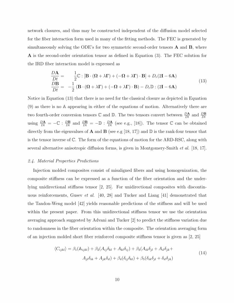
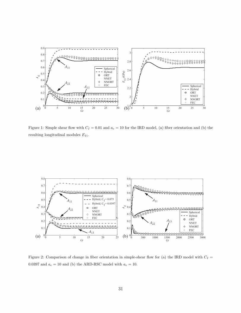
molded parts. The first set of orientation results presented is from the IRD fiber interaction

model for an interaction coefficient of CI = 10−2, a commonly used value of CI , and they are

given in Figure 1(a). The solution using the spherical harmonic approach is numerically exact

and the perfect closure would yield an orientation state that exactly mimics the spherical

harmonic solution. As can be noted in Figure 1(a) the ORT, NNET, NNORT and FEC

are nearly indistinguishable from each other, whereas the hybrid closure significantly over

predicts the alignment state along the x1 axis as indicated by the large A11 values. This

trend is also observed when the orientation is used to predict E11 from the stiffness tensor

using Equation (14), as shown in Figure 1(b). The results in Figure 1(b) are representative

of a solidified composite if the flow were turned off at time Gt. To quantify the error in

predicting the material stiffness component we define the time averaged relative error as the

12

ratio between the spherical harmonic results and the closure results as

χClosureE11=

1

tf − to

∫ tf

to

∣∣∣∣∣ESph11 (t)− EClosure

11 (t)

ESph11 (t)

∣∣∣∣∣ dt× 100% (17)

In the present study, to is the initial flow time and tf is the time when the orientation

is indistinguishable from steady state. The relative error values for E11 presented in the

first column of Table 1 quantifies the observation that the ORT, NNET, NNORT and FEC

closures are more accurate in predicting the stiffness values of the processed composite, in

general, than the Hybrid closure. It is clear from the results for CI = 10−2 that the NNORT

is the best at predicting E11. Similar trends exist for the time averaged relative error for each

of the other stiffness components E22, E33, G23, G13, G12, ν23, ν13 and ν12 computed using a

form similar to Equation (17), and are presented in Table 1. The closure with the greatest

accuracy is bolded in Table 1 for ease of comparison. The basic trend that the NNORT is

the most accurate closure holds for most of the stiffness components with the NNET, ORT

and FEC having similar levels of accuracy. The exception is G13 where the Hybrid closure

is the most accurate by a significant percentage.

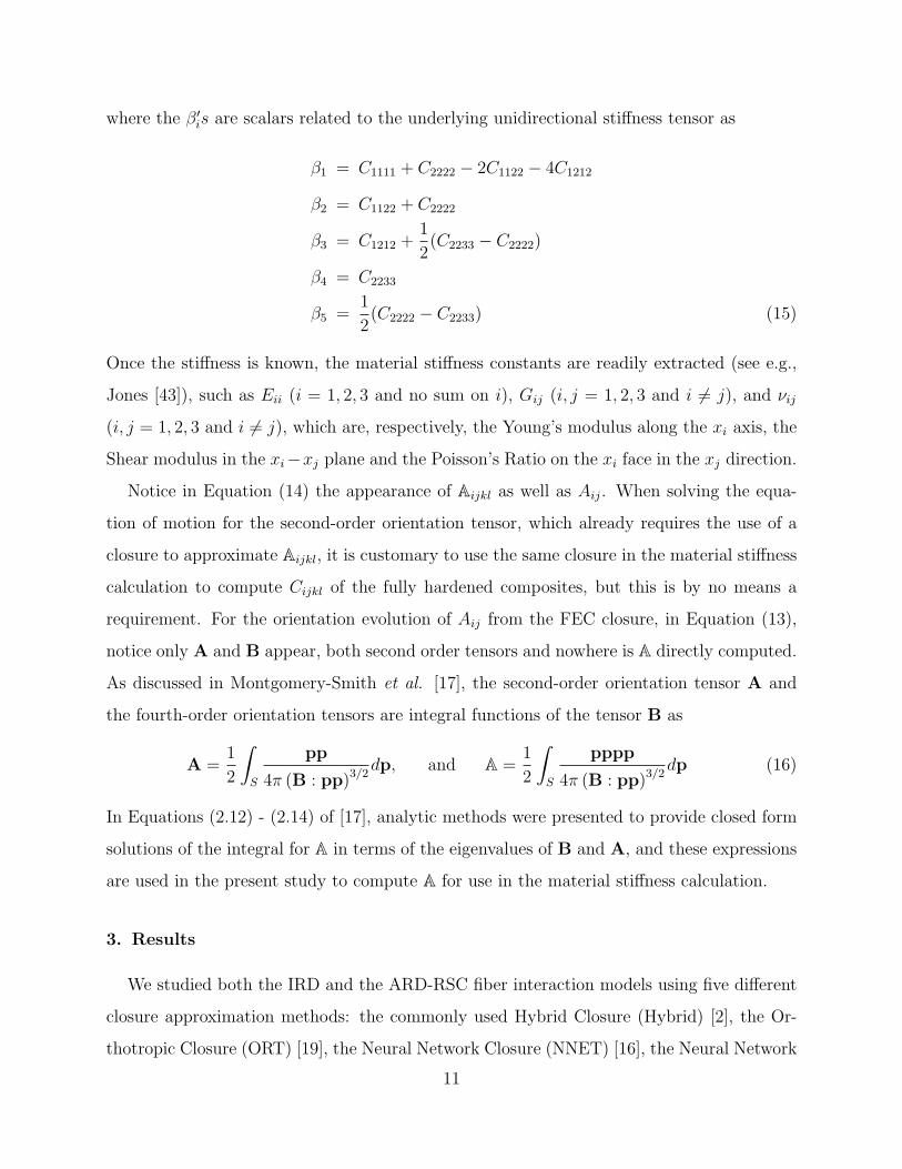
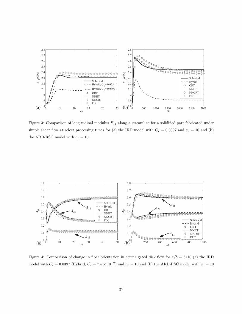
Phelps and Tucker [6] presented their new ARD-RSC closure with coefficients fit based

on experimental observations for a single fiber packing density and fiber aspect ratio. As

observed by the numerical solution of their model in Figure 2(b) the final orientation state is

not the same as was the case for the IRD model results shown in Figure 1 with CI = 10−2. To

compare solutions between the IRD and the ARD-RSC model, we adjusted the interaction

coefficient from the IRD results until the spherical harmonic solutions from both approaches

yielded the same value for A11. We found a value of CI = 3.97 × 10−2 yielded acceptable

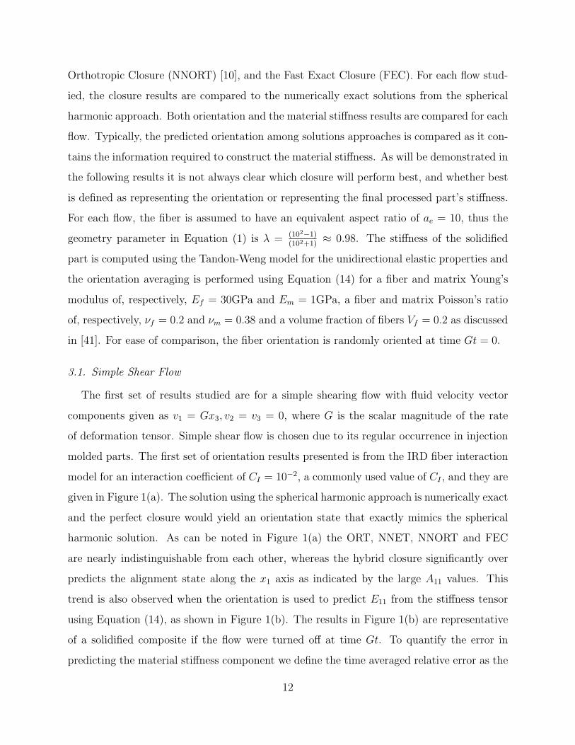
steady state results as observed in Figure 2 for the orientation tensor. For this new interaction

coefficient, the orthotropic closures and the FEC closure for the IRD again yield similar

results to those of the numerically exact spherical harmonic solutions for both orientation

as observed in Figure 2 and for stiffness as observed in Figure 3. Conversely, the Hybrid

close tends to over predict the alignment as noted in Figure 2. As in the previous study

for CI = 10−2, we compute the time average relative error, and as noted in Table 2 the

conclusions are nearly the same as before.

13

3.1.1. Simple Shear Flow - Alignment Over Prediction and the Hybrid Closure

In fairness, the over prediction of alignment from the hybrid closure for the IRD flow

observed in Figure 1(a) and 2(a) is not surprising. Typically in industrial processes the

interaction coefficient for the hybrid closure is selected so that it retains the same steady

state orientation of the principal component of the second-order orientation tensor as would

be expected from the true solution. It was found that CI = 7.5× 10−2 yielded an A11 value

nearly identical to that computed from the orthotropic closures and the spherical harmonic

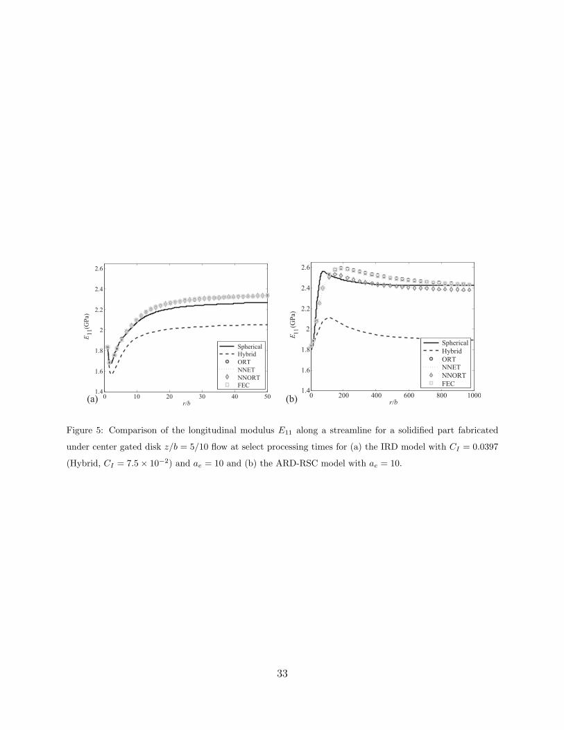
solution using a value of CI = 3.97 × 10−2. What is interesting is how observations of

the relative accuracy of exclusively the A11 parameter do not directly correspond with the

stiffness prediction results for the hybrid closure. This is observed in Figure 3(a) for the

value of E11 predicted from IRD flow using the various closure techniques and the spherical

harmonic solution. Although the Hybrid closure results that a value of CI = 7.5×10−2 yields

a better indication of the orientation state than the value of CI = 3.97 × 10−2, the reverse

is true for the E11 stiffness component. This is counter-intuitive as it is often assumed that

an accurate representation of A11 indicates a more accurate representation of E11, which

appears to not be the case in this scenario with the hybrid closure as noted in Figures 2(a)

and 3(a).

To expand on this thought, we first look at the relationship for E11 as a function of

orientation. E11 can be obtained from the stiffness tensor Cijkl. As depicted in Equation (14),

Cijkl is a function of multiple components of both the second- and the fourth-order orientation

tensors. Thus having only Aij accurately does not insure that one will accurately represent

the stiffness. In fact, accurately representing both A11 and A1111 does not necessarily indicate

an accurate computation of E11. E11 is a function of the compliance tensor Sijkl through the

relationship E11 = 1/S1111, where the compliance tensor Sijkl is the inverse of the stiffness

tensor Cijkl. For an orthotropic form of the stiffness tensor, the E11 and E22 components

can be expressed as

E11 =Det (C)

C1212C1313C2323 (C2222C3333 − C22233)

E22 =Det (C)

C1212C1313C2323 (C1111C3333 − C21133)

(18)

where Det (C) is the tensor determinant of the stiffness tensor Cijkl and will depend on a14

variety of terms from Aij and Aijkl. Notice that with the exception of Det (C), E11 is not a

function of C1111, which is the only term in Cijkl that contains the fourth-order orientation

tensor component A1111, whereas E22 is.

Unfortunately the form of Equation (18) with the expression Det (C) obscures the sensi-

tivity of the stiffness components E11 and E22 to small errors or changes in the orientation

tensor. To further probe the discrepancy for the unusual behavior of the Hybrid results

we take Equation (17) and look at the sensitivity of the expression to small numerical per-

turbations in select components of the stiffness. We do not present the sensitivity of the

time averaged relative error to small changes in Aij as this would explicitly impact Aijkl, as

Aijkl is computed using a closure from Aij. To compute the sensitivity, we run the complete

flow history using a desired closure for CI = 3.97 × 10−2 for the Spherical, Hybrid, ORT,

NNORT, NNET and FEC approaches and CI = 7.5 × 10−2 for the Hybrid approach. We

then perturb one component of Aiiii (no sum on i) for the given orientation states from the

simple shear flow and compute the error from Equation (17). We then use this value to

define the sensitivity (derivative) of the error χE11 to a change in a particular fourth-order

orientation tensor component as

dχE11

dAiiii≃χperturbed

E11− χunperturbed

E11

∆Aiiii(19)

where ∆Aiiii is a small change in a single component of Aijkl. For this test, we set ∆Aiiii =

10−6 for each of the A1111, A2222, and A3333 components. In Table 3 we present the sensitivity

of the error results for the material parameters E11, E22 and E33 to slight variations in the

fourth-order orientation tensor. Looking at thedχE11

dAiiiiterms it is clear that the error for E11

in general is more sensitive to changes in A1111 relative to the E22 and E33 terms, but for the

Hybrid closure with CI = 7.5×10−2 the sensitivity of E11 to small changes in A1111 is nearly

4 times larger than that for the orthotropic closures. Small changes to the A2222 component

effect each of the E11, E22 and E33 components in similar fashions for the orthotropic closures.

For the Hybrid closure a small change to A2222 has a significant impact on E22, as well as the

components E11 and E33. It is expected that due to the preferential alignment along the x1

axis the A1111 component would dominate the error for an approximated orientation state

that is similar to the true orientation state, which is the case for the orthotropic closures.

15

But as the hybrid closure yields an orientation state that is quite dissimilar to the true

orientation state, even when one orientation component is correct, the resulting confidence

in the material stiffness accuracy is not easily quantified.

3.1.2. Simple Shear Flow - Differences Between IRD and ARD-RSC

As observed in Figure 2(b), for the ARD-RSC model the predicted orientation is nearly

indistinguishable between the Hybrid, NNET, NNORT, ORT and FEC for the same interac-

tion parameters b1− b5 from Equation (6). It is worthwhile to note that for the two different

fiber collision models, the IRD and the ARD-RSC, there are significant differences in the

time required for the distribution to attain steady state. For the IRD model this occurs when

Gt ≃ 20 − 25, whereas the ARD-RSC solution requires Gt ≥ 3000. For the IRD and the

ARD-RSC flows the orthotropic and the FEC closures behave in similar fashions in that they

all represent, with reasonable accuracy, both the orientation state and the material stiffness

parameter E11 as observed in Figure 3(b). The hybrid seems to reasonably represent the

orientation state as shown in Figure 2(b) for the ARD-RSC flow, but the error in the E11

stiffness component is significant as demonstrated in Figure 3(b). The average relative error

in the stiffness components is presented for the ARD-RSC results in Table 4. For most of

the stiffness components the neural network closures are the most accurate for the IRD flow,

whereas for the ARD-RSC flow the FEC closure is the most accurate with the ORT falling

a very close second and the NNET and NNORT retaining quite reasonable accuracies. The

accuracy of the Hybrid for most components is not up to the standards of the orthotropic

closures.

3.2. Center-Gated Disk flow

Center-gated disk flow is indicative of the flow field near a pin gate [4, 19, 25], and

regularly occurs in industrial processes. In this type of flow, the fiber suspension enters the

mold through a pin gate and flows radially outward where the velocity vector v = (vr, vθ, vz)

is a function of both the gap height 2b between the wall of the mold and the radial distance

r from the gate. The velocity field and the velocity gradient of a center gated disk for a

16

Newtonian solvent may be represented as

vr =3Q

8πrb

(1−

(zb

)2), vθ = vz = 0

∂vi∂xj

=3Q

8πrb

−1r

(1− z2

b2

)0 −2

bzb

0 1r

(1− z2

b2

)0

0 0 0

(20)

where z is the gap height location between the mold walls with z = 0 taken to be the mid-

plane between the mold walls and Q is the volumetric flow rate. In practice, one would

couple the flow kinetics with the fiber orientation kinematics (see e.g., [21, 22, 19] for how

this might be done), but in the present context, to retain the focus on purely orientational

effects, we leave the coupled problem for various diffusion models to a future study. We made

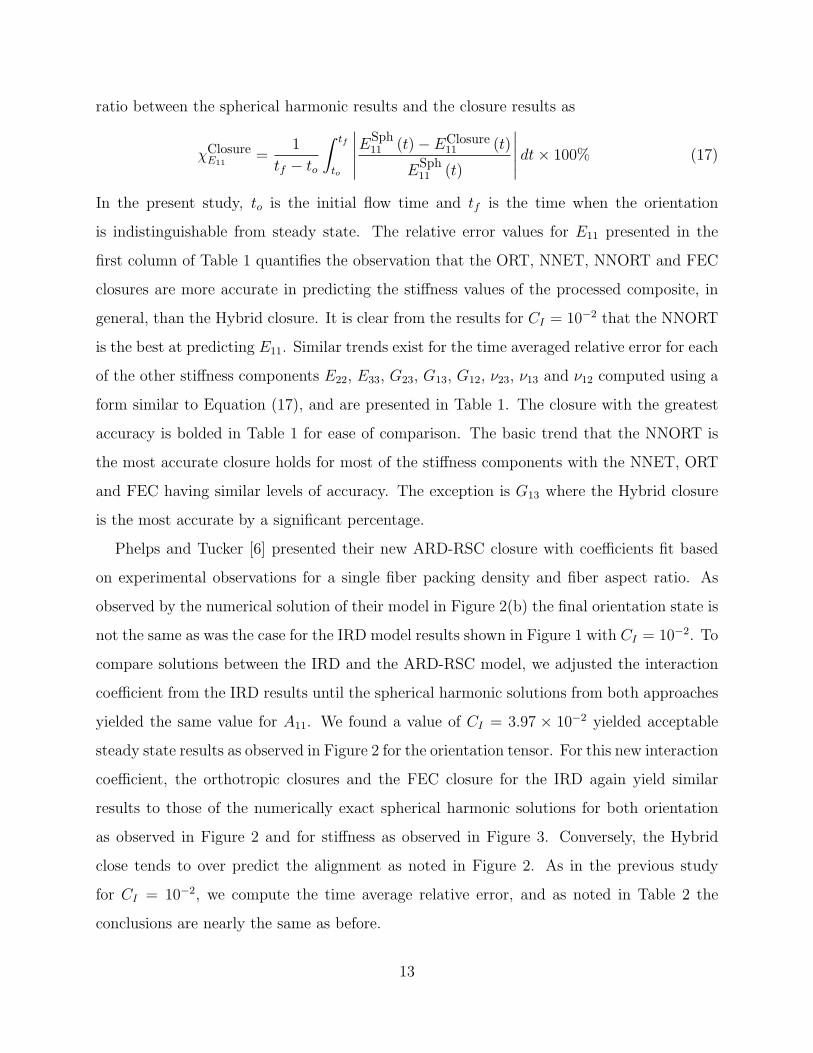
predictions for the streamline along z/b = 5/10 with an initial isotropic fiber orientation at

r/b = 1. The result for A from both the IRD and the ARD-RSC fiber interaction models is

shown in Figure 4, and as in the previous example CI = 3.97× 10−2 (except for the Hybrid,

where we used CI = 7.5× 10−2) to insure the same steady state orientation between the two

fiber interaction models. The observations are quite similar to those from the simple shear

flow where all of the closures reasonably predict the alignment state for both the IRD and

the ARD-RSC results. For both the IRD and ARD-RSC flow, the Hybrid, NNET, NNORT,

ORT and FEC appear to give quite similar results with the NNORT appearing to yield a

slightly better prediction of A. It is interesting to note the predicted material stiffness from

each of the closures over the two different diffusion model flows, as indicated in Figure 5

for E11, as a function of radial distance in the mold. Notice the large initial dip in the E11

component from the IRD model, which is due to the large out-of-plane shear.Conversely,

for the ARD-RSC model, this same large dip does not occur. This is not surprising as

the ARD-RSC model slows the rate of change in the orientation whereby the out-of-plane

shearing only occurs during a small portion of the mold filling, and for increasing values of

r/b the flow is dominated by the radial shearing. Therefore this dip would not be expected

to occur in the ARD-RSC flow model. As in the simple shear flow, the Hybrid predicts the

A11 component for both the IRD and the ARD-RSC flow reasonably well, but significantly

under predicts E11. The stiffness prediction of E11 from the ARD-RSC flow is noted in17

Figure 5(b) where the orientation results from each of the orthotropic and FEC closures

mapped over reasonably well to the stiffness predictions with similar trends. The error for

each of the stiffness components are presented in Table 5 for the IRD model, and unlike the

shear results no closure is clearly the best between the NNET, NNORT, ORT and FEC as

each produce similar error results for each of the investigated stiffness components with one

or the other performing better for various components. It is striking to note that with the

exception of G23 and ν13 the hybrid closure has difficulty in representing the stiffness.

3.3. Thin Geometry Prediction

For the present study we will focus on the lubrication region of a thin plaque and far

from the mold edges. This flow is not a true filling calculation as both the fountain effect

and thermal gradients are neglected. For industrial simulations, the interested reader should

investigate Bay and Tucker [44]. The following example is intended to highlight the differ-

ences between the diffusion models while retaining orientational similarities with a plaque

molded part, i.e., a less oriented core and a slightly oriented shell layer. The thin cavity is

defined as having length l = 10cm and thickness of h = 3.2mm. The flow is fully developed

and pressure driven, with the viscous properties of HDPE polymer (a pseudo plastic). The

shear stress tensor of a pseudo plastic is defined, (see e.g., [45]), by

τij = 2K|2ΓklΓkl|(n−12

)Γij sum on k and l (21)

Γij =1

2(∂vi∂xj

+∂vj∂xi

) (22)

and using Equation (21) and (22), the shear stress τ13 in the thin cavity, with x1 being the

flow direction and x3 the direction of shear, is

τ13 = 2K|∂v1∂x3

|n−1 ∂v1∂x3

(23)

where K is the flow consistency index in units of Pa.sn and n is the flow behavior index

(dimensionless). Using the differential equation for the momentum flux, the second order

partial differential equation of a fully developed simple shear flow in a thin cavity can be

solved to yield the average velocity profile of (see e.g., [11] for the full derivation)

v1 =n

n+ 1

((p1 − p2)

KL

)1/n[(

h

2

)1+ 1n

− |x3|1+1n

](24)

18

Note, the velocity does not change along the flow direction x1, but varies in the x3 direction.

In Equation (24), h is the the thickness of the mold cavity and p1 and p2 are the inlet and

outlet pressures respectively. For our prediction we selected a pressure differential of 100 psi

(69MPa) , K = 2× 10−4 and n = 0.41.

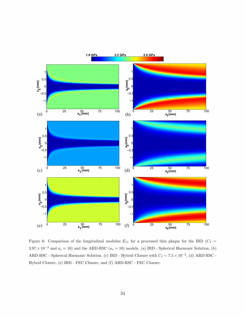
Observing the significant difference in the elastic properties predicted, using both of the

two fiber interaction models, will lend insight to experimentalists for choosing which diffusion

model is more applicable for their system, and should be the scope of a future study. The

longitudinal Young’s moduli E11 are presented in Figure 6 in the left and right column for,

respectively, the IRD and the ARD-RSC model results. In each cavity, the flow enters from

the left side with an initial isotropic orientation state. Along the walls the fibers quickly

align but within the core region the fibers take a significantly longer period to reach any

noticeable change in the alignment as observed by the low E11 values. Notice for the same

geometry and fluid flow profile the two diffusion models demonstrate a remarkable difference

in the spatially varying E11 values. The IRD model predicts somewhat uniform longitudinal

elastic young modulus just a few millimeters from the inlet, whereas the ARD-RSC has

considerable spatial inhomogeneity.

The closure effects for each of the fiber interaction models is also very interesting. For

example there is some difference in E11 values from the closure results as compared to the

spherical solution for the IRD interaction model, as observed by viewing the colors in Figure

6. For the ARD-RSC flow the Hybrid result difference is quite drastic, therefore, having the

orientation correctly (as defined by A alone) is not sufficient for capturing the stiffness. The

FEC results on the other-hand (where the FEC and ORT yield visually identical results in

this example) are quite stable for both fiber interaction models, lending further motivation

to accepting the newer closure.

3.4. Eigenfrequency Analysis

We decided to carry out investigation on the natural frequencies of the simulated thin

plaque in the hopes of observing differences between diffusion models. This was originally

done in the hope that macroscopic experimental analysis techniques might be developed to

quantify the choice of diffusion model, and in particular the rate of alignment within a part.

19

To carry out this eigenfrequency analysis, COMSOL Multiphysics was used to call MAT-

LAB scripts containing the spatially varying stiffness properties based on the orientation

results from solving Equation (4) and (5) for the IRD and the ARD-RSC models respec-

tively. A density of 1000 kg/m3 with a part depth of 1.27mm, height of 3.2mm and length

of 10cm was used for predicting the eigenfrequency of a thin plaque where the inlet side of

the plaque is clamped. The results for the first five natural frequencies using the Hybrid

and the FEC closures (where NNET, NNORT, and ORT results were nearly indistinguish-

able with that of the FEC) as well as the spherical harmonics solution are shown in Figure

7(a) for the IRD model and in Figure 7(b) for the ARD-RSC model result. The FEC and

Hybrid closures yield very similar frequency predictions as that of the spherical harmonics

solution for both models. Clearly from Figure 7 there is very little difference in the natural

frequencies for the two fiber interaction models, even though there is a significant difference

in the stiffness predictions as noted in Figure 6. This seemingly counterintuitive observation

warrants further discussion. The finite element model for the natural frequency prediction

can be expressed as (see e.g., [11])

(KM−1 − ω2I) ∆ = 0 (25)

where ω is the natural frequency, K is the stiffness tensor and M is the mass matrix. From

Equation (25) it can be shown that if the value of stiffness is doubled the eigenfrequency

will only increase by√2 (see e.g., [46, 11]). Consequently, based on the observations of the

moduli in Figure 6 the differences in the stiffness is well below even a factor of two, and

it is not significant enough to warrant the use of natural frequencies to determine the fiber

interaction model for a given fiber suspension.

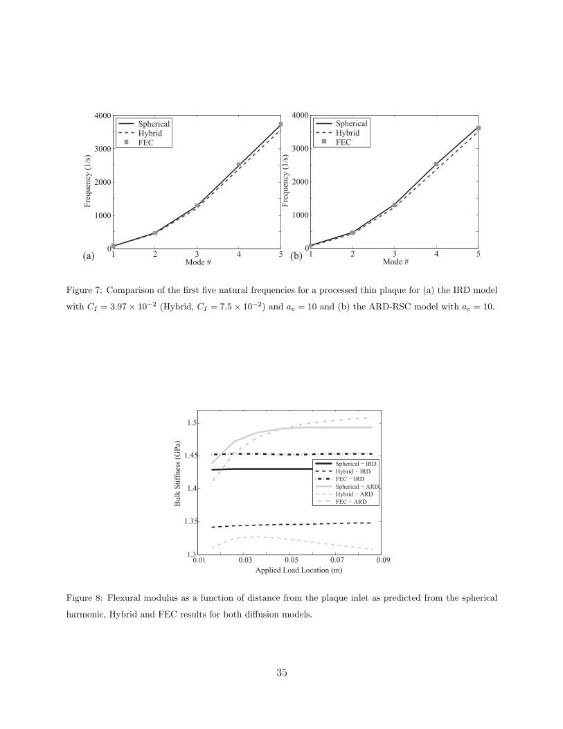
3.5. Flexural Modulus Analysis

The eigenfrequency is obviously insensitive to the fiber orientation change predicted by

the two models. An alternative is the flexural modulus test for the thin plaque. The flexural

modulus is a measure of stiffness of a part and is often used to characterize reinforced plastics.

The flexural modulus (Eb) is typically referred to as the slope of the flexural stress against

the flexural strain in a three-point bending test [47], and is often defined as Eb = FL3/4bh3,

where F is the applied load, L is the length or span of support, b is the depth of the plaque,20

h is the thickness of the plaque. The dimension of the part used for our simulated flexural

test was length×depth×thickness of 10cm×1.27mm×3.2mm chosen in accordance with the

ASTM D790 test fixture [47]. The simulated test was carried out for the IRD and the ARD-

RSC models using the FEC and Hybrid closures along with the spherical harmonic results.

The results for ORT, NNET and NNORT, are not presented because their results and that

of the FEC closure are similar. The finite element analysis was performed using COMSOL

for the three point bend tests. The properties of the part vary spatially, and a single test

cannot be used to capture the changes in the stiffness. A study is performed at regular

intervals in the part to mimic the 3 point bend test fixture, and are presented in Figure 8.

To capture the spatial variation in the stiffness, the three point bend test was performed at

various positions along the plaque, but each test was for the same fixed interval of 1 cm.

This interval was chosen as it was nearly a factor of 10 greater than the part thickness. If

the interval is increased too much, it will be harder to capture local effects, whereas if the

interval is decreased significantly the concept of flexural modulus becomes ambiguous. From

the figure, it can be observed that the flexural moduli values predicted form the ARD-RSC

are significantly different from those predicted by the IRD model. The ARD-RSC result

shows significant changes in the flexural modulus along the length of the beam whereas for

the IRD model, there was no significant change.

We hypothesize that testing the flexural modulus for each section of a molded composite

may be a way to determine which of the two rotary diffusion models is appropriate. For

example, if the percent change in flexural modulus along the global length of the thin plaque

is very low (i.e no significant change), the IRD model may be the appropriate model. On

the other hand, if there is considerable change in the flexural modulus along the length the

ARD-RSC model would be appropriate, and possibly this approach could be used to quantify

the parameter κ used in the ARD-RSC equation of motion. A tangential observation is that

of the Hybrid closure flexural modulus, which increases and then decreases as we move along

the length of the thin plaque, contrary to the predictions for the FEC and the spherical

results. The explanation we found for this difference is that the shear modulus G13 plays

a large role in the value of the flexural modulus. For the Hybrid closure G13 behaved in

a different manner relative to the FEC and the spherical results. For the Hybrid results,

21

G13 showed an initial increase and then a continuous and significant decrease, unlike the

continuous and gradual decrease observed for the FEC and the spherical results.

4. Conclusions

This paper presents two different rotary diffusion mathematical models used for predicting

flow induced orientation of an injection molded short fiber reinforced thermoplastic. Sev-

eral closure approximation methods were used to solve the second-order orientation tensor

equation of motion. In general it was observed that the FEC and the orthotropic closures

performed quite well for each of the flows investigated, with the FEC generally providing

a small improvement in accuracy relative to the orthotropic closures. In this paper, we

demonstrated that using the second-order orientation tensor to infer the accuracy in obtain-

ing a particular stiffness component may be insufficient. In particular, observe the solution

from the ARD-RSC model where the A components from each of the closures are quite

similar, but the resulting fourth-order stiffness tensor has a considerable difference between

the closure predictions with the orthotropic and FEC closures performing with the greatest

accuracy. This paper presented the eigenfrequency approach for possible use in determining

which diffusion model for fiber interactions is more appropriate for a given fiber suspension,

but based on the results presented it appears this is not a viable approach for industrial use

in selecting a diffusion model. Conversely, the flexural modulus results are quite promis-

ing, and our results indicate that this may be a viable experimental approach to confirm

or refute a particular diffusion model and may even aid in the selection of the empirical

parameters for the diffusion model. Our study revealed that there is significant difference

between the ARD-RSC and the IRD models, which provide motivation for further studies

to validate which fiber interaction model is appropriate for commercial predictions of the

resulting stiffness of injection molded short-fiber reinforced composites.

5. Acknowledgements

The authors gratefully acknowledge support from N.S.F. via grant C.M.M.I. 0727399 as

well as Baylor University through their new faculty start-up assistance. The authors are

22

also exceedingly grateful to the reviewers and their suggestion to investigate the flexural

modulus.

23

[1] F. Folgar, C. Tucker, Orientation Behavior of Fibers in Concentrated Suspensions, Jour-

nal of Reinforced Plastics and Composites 3 (1984) 98–119.

[2] S. Advani, C. Tucker, The Use of Tensors to Describe and Predict Fiber Orientation in

Short Fiber Composites, Journal of Rheology 31 (8) (1987) 751–784.

[3] R. Bay, Fiber Orientation in Injection Molded Composites: A Comparison of Theory

and Experiment, Ph.D. thesis, University of Illinois at Urbana-Champaign (August

1991).

[4] J. S. Cintra, C. Tucker, Orthotropic Closure Approximations for Flow-Induced Fiber

Orientation, Journal of Rheology 39 (6) (1995) 1095–1122.

[5] D. Koch, A Model for Orientational Diffusion in Fiber Suspensions, Physics of Fluids

7 (8) (1995) 2086–2088.

[6] J. Phelps, C. Tucker, An Anisotropic Rotary Diffusion Model for Fiber Orienation in

Short- and Long Fiber Thermoplastics, Journal of Non-Newtonian Fluid Mechanics 156

(2009) 165–176.

[7] G. Jeffery, The Motion of Ellipsoidal Particles Immersed in a Viscous Fluid, Proceedings

of the Royal Society of London A 102 (1923) 161–179.

[8] S. Advani, Prediction of Fiber Orientation During Processing of Short Fiber Composites,

Ph.D. thesis, University of Illinois at Urbana-Champaign (August 1987).

[9] D. Jack, D. Smith, An Invariant Based Fitted Closure of the Sixth-order Orientation

Tensor for Modeling Short-Fiber Suspensions, Journal of Rheology 49 (5) (2005) 1091–

1116.

[10] N. Qadir, D. Jack, Modeling Fibre Orientation in Short Fibre Suspensions Using the

Neural Network-Based Orthotropic Closure, Composites, Part A 40 (2009) 1524–1533.

[11] B. Agboola, Investigation of Dense Suspension Rotary Diffusion Models for Fiber Orien-

tation Predictions during Injection Molding of Short-Fiber Reinforced Polymeric Com-

posites, Master’s thesis, Baylor University (August 2011).24

[12] Montgomery-Smith, S.J., D. Jack, D. Smith, A Systematic Approach to Obtaining

Numerical Solutions of Jefferys Type Equations using Spherical Harmonics, Composites,

Part A 41 (2010) 827–835.

[13] M. Doi, Molecular dynamics and rheological properties of concentrated solutions of

rodlike polymers in isotropic and liquid crystalline phases, Journal of Polymer Science

Part B Polymer Physics 19 (1981) 229–243.

[14] G. Hand, A Theory of Anisotropic Fluids, Journal of Fluid Mechanics 13 (1) (1962)

33–46.

[15] V. Verleye, F. Dupret, Prediction of Fiber Orientation in Complex Injection Molded

Parts, in: Developments in Non-Newtonian Flows, 1993, pp. 139–163.

[16] D. Jack, B. Schache, D. Smith, Neural Network Based Closure for Modeling Short-Fiber

Suspensions, Polymer Composites 31 (7) (2010) 1125–1141.

[17] Montgomery-Smith, S.J., W. He, D. Jack, D. Smith, Exact Tensor Closures for the

Three Dimensional Jeffery’s Equation, Journal of Fluid Mechanics 680 (2011) 321–335.

[18] Montgomery-Smith, S.J., D. Jack, D. Smith, The Fast Exact Closure for Jeffery’s Equa-

tion with Diffusion, Journal of Non-Newtonian Fluid Mechanics 166 (2011) 343–353.

[19] B. VerWeyst, T. C. III, Fiber Suspensions in Complex Geometries: Flow-Orientation

Coupling, The Canadian Journal of Chemical Engineering 80 (2002) 1093–1106.

[20] J. Wang, J. O’Gara, C. Tucker, An Objective Model for Slow Orientation Kinetics in

Concentrated Fiber Suspensions: Theory and Rheological Evidence, Journal of Rheol-

ogy 52 (5) (2008) 1179–1200.

[21] S. Dinh, R. Armstrong, A Rheological Equation of State for Semiconcentrated Fiber

Suspensions, Journal of Rheology 28 (3) (1984) 207–227.

[22] G. I. Lipscomb, M. Denn, D. Hur, D. Boger, Flow of Fiber Suspensions in Complex

Geometries, Journal of Non-Newtonian Fluid Mechanics 26 (1988) 297–325.

25

[23] D. Chung, T. Kwon, Numerical Studies of Fiber Suspensions in an Axisymmetric Radial

Diverging Flow: The Effects of Modeling and Numerical Assumptions, Journal of Non-

Newtonian Fluid Mechanics 107 (2002) 67–96.

[24] A. Eberle, G. Velez-Garcia, D. Baird, P. Wapperom, Fiber orientation kinetics of a

concentrated short glass fiber suspension in startup of simple shear flow, Journal of

Non-Newtonian Fluid Mechanics 165 (2010) 110–119.

[25] D. Jack, D. Smith, Elastic Properties of Short-Fiber Polymer Composites, Derivation

and Demonstration of Analytical Forms for Expectation and Variance from Orientation

Tensors, Journal of Composite Materials 42 (3) (2008) 277–308.

[26] E. Caselman, Elastic Property Prediction of Short Fiber Composites Using a Uniform

Mesh Finite Element Method, Master’s thesis, University of Missouri - Columbia (De-

cember 2007).

[27] A. Gusev, M. Heggli, H. Lusti, P. Hine, Orientation Averaging for Stiffness and Thermal

Expansion of Short Fiber Composites, Advanced Engineering Materials 4 (12) (2002)

931–933.

[28] A. Gusev, H. Lusti, P. Hine, Stiffness and Thermal Expansion of Short Fiber Compos-

ites with Fully Aligned Fibers, Advanced Engineering Materials 4 (12) (2002) 927–930.

[29] N. Nguyen, S. Bapanapalli, V. Kunc, J. Phelps, C. Tucker, Prediction of the Elastic-

Plastic Stress/Strain Response for Injection-Molded Long-Fiber Thermoplastics, Jour-

nal of Composite Materials 43 (3) (2009) 217–246.

[30] R. B. Bird, C. Curtiss, R. C. Armstrong, O. Hassager, Dynamics of Polymeric Liquids,

2nd Edition, Vol. 2: Kinetic Theory, John Wiley & Sons, Inc., New York, NY, 1987.

[31] D. Zhang, D. Smith, D. Jack, S. Montgomery-Smith, Numerical Evaluation of Single

Fiber Motion for Short-Fiber-Reinforced Composite Materials Processing, Journal of

Manufacturing Science and Engineering 133 (5) (2011) 051002–9.

26

[32] D. Jack, Advanced Analysis of Short-fiber Polymer Composite Material Behavior, Ph.D.

thesis, University of Missouri - Columbia (December 2006).

[33] X. Fan, N. Phan-Thien, R. Zheng, A Direct Simulation of Fibre Suspensions, Journal

of Non-Newtonian Fluid Mechanics 74 (1998) 113–135.

[34] N. Phan-Thien, X.-J. Fan, R. Tanner, R. Zheng, Folgar-Tucker Constant for a Fibre Sus-

pension in a Newtonian Fluid, Journal of Non-Newtonian Fluid Mechanics 103 (2002)

251–260.

[35] S. Advani, C. Tucker, Closure Approximations for Three-Dimensional Structure Tensors,

Journal of Rheology 34 (3) (1990) 367–386.

[36] K.-H. Han, Y.-T. Im, Numerical Simulation of Three-Dimensional Fiber Orientation in

Short-Fiber-Reinforced Injection-Molded Parts, Journal of Materials Processing Tech-

nology 124 (2002) 366–371.

[37] D. Chung, T. Kwon, Improved Model of Orthotropic Closure Approximation for Flow

Induced Fiber Orientation, Polymer Composites 22 (5) (2001) 636–649.

[38] D. Chung, T. Kwon, Invariant-Based Optimal Fitting Closure Approximation for the

Numerical Prediction of Flow-Induced Fiber Orientation, Journal of Rheology 46 (1)

(2002) 169–194.

[39] D. Dray, P. Gilormini, G. Regnier, Comparison of Several Closure Approximations for

Evaluating the Thermoelastic Properties of an Injection Molded Short-Fiber Composite,

Composites Science and Technology 67 (7-8) (2007) 1601–1610.

[40] A. Gusev, P. Hine, W. I.M., Fiber Packing and Elastic Properties of a Transversely

Random Unidirectional Glass/Epoxy Composite, Composites Science and Technology

60 (2000) 535–541.

[41] C. Tucker, E. Liang, Stiffness Predictions for Unidirectional Short-Fiber Composites:

Review and Evaluation, Composites Science and Technology 59 (1999) 655–671.

27

[42] G. Tandon, G. Weng, The Effect of Aspect Ratio of Inclusions on the Elastic Properties

of Unidirectionally Aligned Composites, Polymer Composites 5 (4) (1984) 327–333.

[43] R. Jones, Mechanics of Composite Materials: Second Edition, Taylor and Francis, Inc.,

Philadelphia, PA, 1999.

[44] R. Bay, C. Tucker, Fiber Orientation in Simple Injection Moldings: Part 1 - Theory

and Numerical Methods, in: V. Stokes (Ed.), Plastics and Plastic Composites: Material

Properties, Part Performance, and Process Simulation, ASME 1991, Vol. 29, American

Society of Mechanical Engineers, 1991, pp. 445–471.

[45] A. Ishak, N. Bachok, Power-Law Fluid Flow On a Moving Wall, European Journal of

Scientific Research 34 (1) (2009) 55–60.

[46] J. Reddy, An Introduction to the Finite Element Method, Third Edition, McGraw-Hill,

New York, NY, 2006.

[47] ASM Handbook: Mechanical Testing and Evaluation , Vol. 8, ASM International, West

Sussex, England, 2000.

28

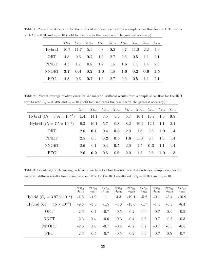
Table 1: Percent relative error for the material stiffness results from a simple shear flow for the IRD results

with CI = 0.01 and ae = 10 (bold font indicates the result with the greatest accuracy).

χE11 χE22 χE33 χG23 χG13 χG12 χν12 χν13 χν23

Hybrid 10.7 11.7 5.1 6.8 0.3 3.7 11.0 2.2 4.3

ORT 4.8 0.6 0.2 1.3 2.7 2.6 0.5 1.1 2.1

NNET 4.3 1.7 0.5 1.2 1.5 1.6 1.1 1.4 2.0

NNORT 3.7 0.4 0.2 1.0 1.8 1.6 0.2 0.9 1.5

FEC 4.8 0.6 0.2 1.3 2.7 2.6 0.5 1.1 2.1

Table 2: Percent average relative error for the material stiffness results from a simple shear flow for the IRD

results with CI = 0.0397 and ae = 10 (bold font indicates the result with the greatest accuracy).

χE11 χE22 χE33 χG23 χG13 χG12 χν12 χν13 χν23

Hybrid (CI = 3.97× 10−2) 1.4 14.1 7.5 5.5 5.7 10.4 18.7 1.5 0.9

Hybrid (CI = 7.5× 10−2) 9.3 10.1 5.7 0.8 8.2 10.2 12.1 1.1 3.4

ORT 2.6 0.1 0.4 0.5 2.0 1.6 0.5 1.0 1.4

NNET 2.5 0.3 0.2 0.5 1.8 1.0 0.4 1.3 1.4

NNORT 2.6 0.1 0.4 0.5 2.0 1.5 0.3 1.1 1.4

FEC 2.6 0.2 0.5 0.6 2.0 1.7 0.5 1.0 1.3

Table 3: Sensitivity of the average relative error to select fourth-order orientation tensor components for the

material stiffness results from a simple shear flow for the IRD results with CI = 0.0397 and ae = 10 .

dχE11

A1111

dχE22

A1111

dχE33

A1111

dχE11

A2222

dχE22

A2222

dχE33

A2222

dχE11

A3333

dχE22

A3333

dχE33

A3333

Hybrid (CI = 3.97× 10−2) -1.5 -1.9 1 3.3 -19.1 -5.2 -0.1 -3.4 -10.9

Hybrid (CI = 7.5× 10−2) -9.5 -3.5 -1.5 -4.8 -13.6 -1.7 -1.4 -0.8 -8.4

ORT -2.6 -0.4 -0.7 -0.5 -0.2 0.6 -0.7 0.4 -0.5

NNET -2.6 0.4 -0.6 -0.3 -0.4 0.6 -0.7 -0.6 -0.3

NNORT -2.6 0.4 -0.7 -0.4 -0.2 0.7 -0.7 -0.5 -0.5

FEC -2.6 -0.5 -0.7 -0.5 -0.2 0.6 -0.7 0.5 -0.7

29

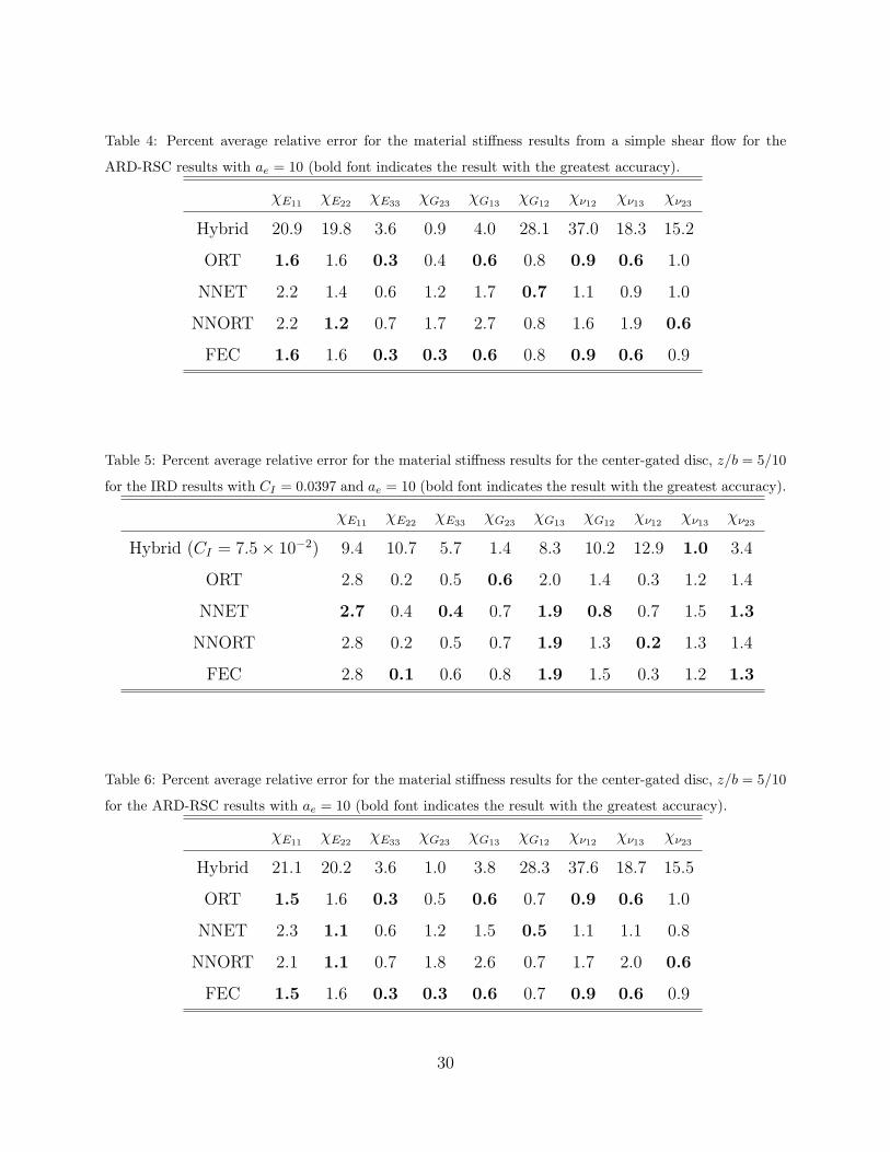
Table 4: Percent average relative error for the material stiffness results from a simple shear flow for the

ARD-RSC results with ae = 10 (bold font indicates the result with the greatest accuracy).

χE11 χE22 χE33 χG23 χG13 χG12 χν12 χν13 χν23

Hybrid 20.9 19.8 3.6 0.9 4.0 28.1 37.0 18.3 15.2

ORT 1.6 1.6 0.3 0.4 0.6 0.8 0.9 0.6 1.0

NNET 2.2 1.4 0.6 1.2 1.7 0.7 1.1 0.9 1.0

NNORT 2.2 1.2 0.7 1.7 2.7 0.8 1.6 1.9 0.6

FEC 1.6 1.6 0.3 0.3 0.6 0.8 0.9 0.6 0.9

Table 5: Percent average relative error for the material stiffness results for the center-gated disc, z/b = 5/10

for the IRD results with CI = 0.0397 and ae = 10 (bold font indicates the result with the greatest accuracy).

χE11 χE22 χE33 χG23 χG13 χG12 χν12 χν13 χν23

Hybrid (CI = 7.5× 10−2) 9.4 10.7 5.7 1.4 8.3 10.2 12.9 1.0 3.4

ORT 2.8 0.2 0.5 0.6 2.0 1.4 0.3 1.2 1.4

NNET 2.7 0.4 0.4 0.7 1.9 0.8 0.7 1.5 1.3

NNORT 2.8 0.2 0.5 0.7 1.9 1.3 0.2 1.3 1.4

FEC 2.8 0.1 0.6 0.8 1.9 1.5 0.3 1.2 1.3

Table 6: Percent average relative error for the material stiffness results for the center-gated disc, z/b = 5/10

for the ARD-RSC results with ae = 10 (bold font indicates the result with the greatest accuracy).

χE11 χE22 χE33 χG23 χG13 χG12 χν12 χν13 χν23

Hybrid 21.1 20.2 3.6 1.0 3.8 28.3 37.6 18.7 15.5

ORT 1.5 1.6 0.3 0.5 0.6 0.7 0.9 0.6 1.0

NNET 2.3 1.1 0.6 1.2 1.5 0.5 1.1 1.1 0.8

NNORT 2.1 1.1 0.7 1.8 2.6 0.7 1.7 2.0 0.6

FEC 1.5 1.6 0.3 0.3 0.6 0.7 0.9 0.6 0.9

30

0 5 10 15 20 25 300

0.1

0.2

0.3

0.4

0.5

0.6

0.7

0.8

0.9

Gt

Aij

Spherical

Hybrid

ORT

NNET

NNORT

FEC

A11

A22A13

0 5 10 15 20 25 301.8

2

2.2

2.4

2.6

2.8

3

Gt

E11 (

GP

a)

Spherical

Hybrid

ORT

NNET

NNORT

FEC

(a) (b)

Figure 1: Simple shear flow with CI = 0.01 and ae = 10 for the IRD model, (a) fiber orientation and (b) the

resulting longitudinal modules E11.

(a) (b) 0 500 1000 1500 2000 2500 30000

0.1

0.2

0.3

0.4

0.5

0.6

0.7

0.8

Gt

Aij

Spherical

Hybrid

ORT

NNET

NNORT

FEC

0 5 10 15 20 250

0.1

0.2

0.3

0.4

0.5

0.6

0.7

0.8

Gt

A11

Spherical Hybrid, C

I = 0.075

Hybrid, CI = 0.0397

ORT

NNET

NNORT

FEC

A11

A22

A13

A11

A22A13

Figure 2: Comparison of change in fiber orientation in simple-shear flow for (a) the IRD model with CI =

0.0397 and ae = 10 and (b) the ARD-RSC model with ae = 10.

31

0 500 1000 1500 2000 2500 30001.8

1.9

2

2.1

2.2

2.3

2.4

2.5

2.6

2.7

2.8

Gt

E11 (

GP

a)

Spherical

Hybrid

ORT

NNET

NNORT

FEC

0 5 10 15 20 251.8

1.9

2

2.1

2.2

2.3

2.4

2.5

2.6

2.7

2.8

Gt

E11 (

GP

a)

Spherical Hybrid, C

I = 0.075

Hybrid, CI = 0.0397

ORT

NNET

NNORT

FEC

(a) (b)

Figure 3: Comparison of longitudinal modulus E11 along a streamline for a solidified part fabricated under

simple shear flow at select processing times for (a) the IRD model with CI = 0.0397 and ae = 10 and (b)

the ARD-RSC model with ae = 10.

0 10 20 30 40 500

0.1

0.2

0.3

0.4

0.5

0.6

0.7

0.8

r/b

Aij

Spherical

Hybrid

ORT

NNET

NNORT

FEC

0 200 400 600 800 10000

0.1

0.2

0.3

0.4

0.5

0.6

0.7

0.8

r/b

Aij

Spherical Hybrid ORT NNET NNORT FEC

(a) (b)

A11A22

A13

A11A22

A13

Figure 4: Comparison of change in fiber orientation in center gated disk flow for z/b = 5/10 (a) the IRD

model with CI = 0.0397 (Hybrid, CI = 7.5× 10−2) and ae = 10 and (b) the ARD-RSC model with ae = 10

32

0 200 400 600 800 10001.4

1.6

1.8

2

2.2

2.4

2.6

r/b

E1

1 (G

Pa)

Spherical

Hybrid

ORT NNET

NNORT

FEC

(a) (b)0 10 20 30 40 501.4

1.6

1.8

2

2.2

2.4

2.6

r/b

E11 (

GP

a)

Spherical

Hybrid

ORT

NNET

NNORT

FEC

Figure 5: Comparison of the longitudinal modulus E11 along a streamline for a solidified part fabricated

under center gated disk z/b = 5/10 flow at select processing times for (a) the IRD model with CI = 0.0397

(Hybrid, CI = 7.5× 10−2) and ae = 10 and (b) the ARD-RSC model with ae = 10.

33

1.8 GPa 2.2 GPa 2.6 GPa

x1 (mm)

x2 (

mm

)

0 25 50 75 100

−1

−0.5

0

0.5

1

x1 (mm)

x2 (

mm

)

0 25 50 75 100

−1

−0.5

0

0.5

1

x1 (mm)

x2 (

mm

)

0 25 50 75 100

−1

−0.5

0

0.5

1

x1 (mm)

x2 (

mm

)

0 25 50 75 100

−1

−0.5

0

0.5

1

x1 (mm)

x2 (

mm

)

0 25 50 75 100

−1

−0.5

0

0.5

1

x1 (mm)

x2 (

mm

)

0 25 50 75 100

−1

−0.5

0

0.5

1

(a) (b)

(c) (d)

(e) (f)

Figure 6: Comparison of the longitudinal modulus E11 for a processed thin plaque for the IRD (CI =

3.97× 10−2 and ae = 10) and the ARD-RSC (ae = 10) models. (a) IRD - Spherical Harmonic Solution, (b)

ARD-RSC - Spherical Harmonic Solution, (c) IRD - Hybrid Closure with CI = 7.5× 10−2, (d) ARD-RSC -

Hybrid Closure, (e) IRD - FEC Closure, and (f) ARD-RSC - FEC Closure.

34

1 2 3 4 50

1000

2000

3000

4000

Mode #

Fre

qu

ency

(1

/s)

Spherical Hybrid FEC

(a) (b) 1 2 3 4 50

1000

2000

3000

4000

Mode #

Fre

qu

ency

(1

/s)

Spherical Hybrid FEC

Figure 7: Comparison of the first five natural frequencies for a processed thin plaque for (a) the IRD model

with CI = 3.97× 10−2 (Hybrid, CI = 7.5× 10−2) and ae = 10 and (b) the ARD-RSC model with ae = 10.

0.01 0.03 0.05 0.07 0.091.3

1.35

1.4

1.45

1.5

Applied Load Location (m)

Bu

lk S

tiff

nes

s (G

Pa)

Spherical − IRD

Hybrid − IRD

FEC − IRD

Spherical − ARD

Hybrid − ARD

FEC − ARD

Figure 8: Flexural modulus as a function of distance from the plaque inlet as predicted from the spherical

harmonic, Hybrid and FEC results for both diffusion models.

35