PREDICTING CLIMATE TIPPING AS A NOISY BIFURCATION: A …

March 10, 2011 11:27 WSPC/S0218-1274 02851

International Journal of Bifurcation and Chaos, Vol. 21, No. 2 (2011) 399–423c© World Scientific Publishing CompanyDOI: 10.1142/S0218127411028519

PREDICTING CLIMATE TIPPING AS ANOISY BIFURCATION: A REVIEW

J. MICHAEL T. THOMPSONDepartment of Applied Mathematics & Theoretical Physics,Cambridge University, Centre for Mathematical Sciences,

Wilberforce Road, Cambridge, CB3 0WA, UKSchool of Engineering (Sixth Century Professor),

Aberdeen University, [email protected]

JAN SIEBERDepartment of Mathematics, University of Portsmouth,

Portsmouth, PO1 3HF, [email protected]

Received March 1, 2010

There is currently much interest in examining climatic tipping points, to see if it is feasible topredict them in advance. Using techniques from bifurcation theory, recent work looks for a slow-ing down of the intrinsic transient responses, which is predicted to occur before an instabilityis encountered. This is done, for example, by determining the short-term autocorrelation coeffi-cient ARC(1) in a sliding window of the time-series: this stability coefficient should increase tounity at tipping. Such studies have been made both on climatic computer models and on realpaleoclimate data preceding ancient tipping events. The latter employ reconstituted time-seriesprovided by ice cores, sediments, etc., and seek to establish whether the actual tipping couldhave been accurately predicted in advance. One such example is the end of the Younger Dryasevent, about 11 500 years ago, when the Arctic warmed by 7◦C in 50 yrs. A second gives an excel-lent prediction for the end of “greenhouse” Earth about 34 million years ago when the climatetipped from a tropical state into an icehouse state, using data from tropical Pacific sedimentcores. This prediction science is very young, but some encouraging results are already beingobtained. Future analyses will clearly need to embrace both real data from improved monitoringinstruments, and simulation data generated from increasingly sophisticated predictive models.

Keywords : Climate tipping; bifurcation prediction; time-series analysis.

1. Introduction

Predicting the future climate is now a major chal-lenge to the world, as witnessed by the recentCopenhagen Conference and its sequels. In study-ing changes to the Earth’s climate, perhaps themost important feature to watch out for, and tryto anticipate, is a so-called tipping point at whichthe climate makes a sudden, and often irreversible,

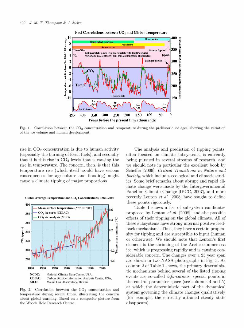
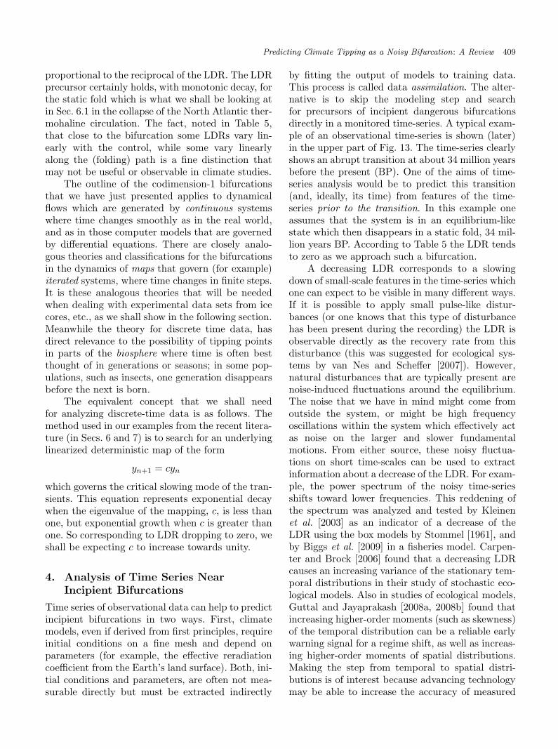
change. Major events of this type are well doc-umented in geological records, striking examplesbeing the on-and-off switching of prehistoric iceages, as illustrated in Fig. 1. The current reason forconcern is the apparently coordinated increase ofthe average global temperature and the percentageof carbon dioxide in the atmosphere, as illustratedin Fig. 2. Many scientists believe, firstly, that the

399

http://dx.doi.org/10.1142/S0218127411028519

March 10, 2011 11:27 WSPC/S0218-1274 02851

400 J. M. T. Thompson & J. Sieber

Fig. 1. Correlation between the CO2 concentration and temperature during the prehistoric ice ages, showing the variationof the ice volume and human development.

rise in CO2 concentration is due to human activity(especially the burning of fossil fuels), and secondlythat it is this rise in CO2 levels that is causing therise in temperature. The concern, then, is that thistemperature rise (which itself would have seriousconsequences for agriculture and flooding) mightcause a climate tipping of major proportions.

280

300

320

340

360

380

400

1880 1900 1920 1940 1960 1980 2000

−0.4

−0.2

0

0.2

0.4

0.6

Global Average Temperature and CO2 Concentrations, 1880–2006

CO

2 (p

pmv)

Tem

pera

ture

Ano

mal

y (°

C)

Mean surface temperature (∆°C, NCDC)

CO2 ice cores (CDIAC)

CO2 air analysis (MLO)

NCDC: National Climate Data Center, USA,CDIAC: Carbon Dioxide Information Analysis Center, USA,MLO: Mauna Loa Observatory, Hawaii.

Fig. 2. Correlation between the CO2 concentration andtemperature during recent times, illustrating the concernabout global warming. Based on a composite picture fromthe Woods Hole Research Centre.

The analysis and prediction of tipping points,often focused on climate subsystems, is currentlybeing pursued in several streams of research, andwe should note in particular the excellent book byScheffer [2009], Critical Transitions in Nature andSociety, which includes ecological and climatic stud-ies. Some brief remarks about abrupt and rapid cli-mate change were made by the IntergovernmentalPanel on Climate Change [IPCC, 2007], and morerecently Lenton et al. [2008] have sought to definethese points rigorously.

Table 1 shows a list of subsystem candidatesproposed by Lenton et al. [2008], and the possibleeffects of their tipping on the global climate. All ofthese subsystems have strong internal positive feed-back mechanisms. Thus, they have a certain propen-sity for tipping and are susceptible to input (humanor otherwise). We should note that Lenton’s firstelement is the shrinking of the Arctic summer seaice, which is progressing rapidly and is causing con-siderable concern. The changes over a 23 year spanare shown in two NASA photographs in Fig. 3. Ascolumn 2 of Table 1 shows, the primary determinis-tic mechanisms behind several of the listed tippingevents are so-called bifurcations, special points inthe control parameter space (see columns 4 and 5)at which the deterministic part of the dynamicalsystem governing the climate changes qualitatively(for example, the currently attained steady statedisappears).

March 10, 2011 11:27 WSPC/S0218-1274 02851

Table

1.

Sum

mary

ofLen

ton’s

Tip

pin

gE

lem

ents

,nam

ely

clim

ate

subsy

stem

sth

at

are

likel

yto

be

candid

ate

sfo

rfu

ture

tippin

gw

ith

rele

vance

topoliti

caldec

isio

nm

akin

g.In

colu

mn

2,th

eposs

ibility

ofth

ere

bei

ng

an

under

lyin

gbifurc

ati

on

isin

dic

ate

das

follow

s:bla

ck=

hig

h,gre

y=

med

ium

,w

hit

e=

low

.N

oti

ceth

at

inco

lum

n4

EE

Pden

ote

sth

eE

ast

ern

Equato

rialPaci

fic

and

inth

ela

stco

lum

nIT

CZ

den

ote

sth

eIn

tert

ropic

alC

onver

gen

ceZone.

This

list

willbe

discu

ssed

ingre

ate

rdet

ail

inSec

.5.

Tip

pin

gE

lem

ent

Fea

ture

,F

(Change)

Contr

olPara

met

er,µ

µcri

tG

lobalW

arm

ing

Tra

nsi

tion

Tim

e,T

Key

Impact

s

Arc

tic

sum

mer

sea-ice

Are

alex

tent

(−)

Loca

l∆

Tair,oce

an

hea

ttr

ansp

ort

??+

0.5

to+

2◦ C

∼10

yrs

(rapid

)A

mplified

warm

ing,

ecosy

stem

change

Gre

enla

nd

ice

shee

t(G

IS)

Ice

volu

me

(−)

Loca

l∆

Tair

∼+

3◦ C

+1

to+

2◦ C

>300

yrs

(slo

w)

Sea

level

+2

to+

7m

Wes

tanta

rctic

ice

shee

t(W

AIS

)Ic

evolu

me

(−)

Loca

l∆

Tair

or,

less

∆T

ocean

+5

to+

8◦ C

+3

to+

5◦ C

>300

yrs

(slo

w)

Sea

level

+5

m

Atl

anti

cth

erm

ohaline

circ

ula

tion

Over

turn

ing

(−)

Fre

shw

ate

rin

put

toN

ort

hA

tlanti

c+

0.1

to+

0.5

Sv

+3

to+

5◦ C

∼100

yrs

(gra

dual)

Reg

ionalco

oling,se

ale

vel

,IT

CZ

shift

ElN

ino

South

ern

osc

illa

tion

Am

plitu

de

(+)

Ther

mocl

ine

dep

th,

sharp

nes

sin

EE

P??

+3

to+

6◦ C

∼100

yrs

(gra

dual)

Dro

ught

inSE

Asia

and

else

wher

e

India

nsu

mm

erm

onso

on

(ISM

)R

ain

fall

(−)

Pla

net

ary

alb

edo

over

India

0.5

N/A

∼1yr

(rapid

)D

rought,

dec

rease

dca

rryin

gca

paci

ty

Sahara

/Sahel

and

W.A

fric

an

monso

on

Veg

etati

on

fract

ion

(+)

Pre

cipit

ati

on

100

mm

/yr

+3

to+

5◦ C

∼10

yrs

(rapid

)In

crea

sed

carr

yin

gca

paci

ty

Am

azo

nra

in-fore

stTre

efr

act

ion

(−)

Pre

cipitation,dry

seaso

nle

ngth

1100

mm

/yr

+3

to+

4◦ C

∼50

yrs

(gra

dual)

Bio

div

ersity

loss

,dec

rease

dra

infa

ll

Bore

alfo

rest

Tre

efr

act

ion

(−)

Loca

l∆

Tair

∼+

7◦ C

+3

to+

5◦ C

∼50

yrs

(gra

dual)

Change

inty

pe

ofth

eec

osy

stem

401

March 10, 2011 11:27 WSPC/S0218-1274 02851


Fig. 3. Two NASA satellite photographs, showing thereduction of Arctic snow and ice cover over a 23 yrs interval.Source: http://nasascience.nasa.gov/images/about-us/accom-plishments/YIR2004 arctic.jpg.

In Sec. 3 we review possible bifurcations andclassify them into three types, safe, explosive anddangerous. Almost universally these bifurcationshave a precursor: in at least one mode, all feedbackeffects cancel at the linear level, which means thatthe system is slowing down, and the local (or lin-ear) decay rate (LDR) to the steady state decreasesto zero.

Most of the relevant research is devoted tocreating climate models from first principles, tun-ing and initializing these models by assimilat-ing geological data, and then running simulationsof these models to predict the future. Climatemodels come in varying degrees of sophisticationand realism, more complex ones employing up to3 × 108 variables [Dijkstra, 2008]. Predictions donot rely solely on a single “best model” start-ing from the “real initial conditions”. Typically,all qualified models are run from ensembles ofinitial conditions and then a statistical analysisover all generated outcomes is performed [IPCC,2007].

An alternative to the model and simulateapproach (and in some sense a short-cut) is to real-ize that mathematically some of the climate-tippingevents correspond to bifurcations (see Sec. 3 fora discussion), and then to use time-series analysistechniques to extract precursors of these bifurca-tions directly from observational data. This method

still benefits from the modeling efforts becausesimulations generated by predictive models allowanalysts to hone their prediction techniques onmasses of high quality data, with the possibilityof seeing whether they can predict what the com-puter eventually displays as the outcome of itsrun. Transferring these techniques to real data fromthe Earth itself is undoubtedly challenging. Still,bifurcation predictions directly from real time-serieswill be a useful complement to modeling from firstprinciples because they do not suffer from all themany difficulties of building and initializing reliablecomputer models. Our review discusses the currentstate of bifurcational predictions in climate time-series, focusing on methods introduced by Held andKleinen [2004] and Livina and Lenton [2007]. Heldand Kleinen analyze the collapse of the global con-veyor belt of oceanic water, the thermohaline circu-lation (THC). This conveyor is important, not onlyfor the water transport, per se, but because of theheat and salt that it redistributes.

The paper by Livina and Lenton [2007] isparticularly noteworthy in that it includes whatseems to be the first bifurcational predictions usingreal data, namely the Greenland ice-core paleo-temperature data spanning the time from 50 000years ago to the present. The unevenly spaced datacomprised 1586 points and their DFA-propagator(this quantity reaches +1 when the local decay ratevanishes; see Sec. 4.1) was calculated in sliding win-dows of length 500 data points. The results areshown in Fig. 4, and the rapid warming at the end ofthe Younger Dryas event, around 11 500 yrs beforethe present is anticipated by an upward trend inthe propagator, which is heading towards its crit-ical value of +1 at about the correct time. Withthe data set running over tens of thousands ofyears, this study should be seen primarily as anestimate of the end of the last glaciation, ratherthan the Younger Dryas event itself. The slidingwindow that ends near the tipping is highlighted,and we note that (as we emphasize at the endof Sec. 4.1), from a prediction point of view, thepropagator estimates would end at point A. Thegrey propagator curve beyond A uses time-seriespoints beyond the tipping point, which would notnormally be available: in any event, they shouldnot be used, because they contaminate the greyresults with data from a totally different climaticstate.

In a second notable paper, Dakos et al. [2008]systematically estimated the LDR for real data in

March 10, 2011 11:27 WSPC/S0218-1274 02851

Predicting Climate Tipping as a Noisy Bifurcation: A Review 403D

FA

1 P

ropa

gato

rT

empe

ratu

re (

°C)

Asliding window

40,000

−20

−30

−40

−50

−60

0.6

0.8

1.0

30,000 20,000 10,000 0

End of the

Younger Dryas

Target

Years before the present

End of last glaciation: using ice-core paleo-temperatures

Fig. 4. Results of Livina and Lenton [2007] for the endof the last glaciation (a) Greenland ice-core (GISP2) paleo-temperature with an unevenly spaced record, visible in thevarying density of symbols on the curve. The total number ofdata points is N = 1586. In (b) the DFA1-propagator is cal-culated in sliding windows of length 500 points and mappedinto the middle points of the windows. The results of a sec-ond and much more local study by Dakos et al. [2008] (thatwe shall be discussing in Fig. 14) are highlighted by the redcircle.

their analysis of eight ancient tipping events viareconstructed time-series. These are:

(a) the end of the greenhouse Earth about 34 mil-lion years ago when the climate tipped from atropical state (which had existed for hundredsof millions of years) into an icehouse state withice caps, using data from tropical Pacific sedi-ment cores,

(b) the end of the last glaciation, and the ends ofthree earlier glaciations, drawing data from theAntarctica Vostok ice core,

(c) the Bølling–Allerod transition which was datedabout 14 000 years ago, using data from theGreenland GISP2 ice core,

(d) the end of the Younger Dryas event about11 500 years ago when the Arctic warmed by7◦C in 50 yrs, drawing on data from the sed-iment of the Cariaco basin in Venezuela. Thisexamines at a much shorter time-scale, and withdifferent data, the transition of Fig. 4,

(e) the desertification of North Africa when therewas a sudden shift from a savanna-like statewith scattered lakes to a desert about 5000years ago, using the sediment core from ODPHole 658C, off the west coast of Africa.

In all of these cases, the dynamics of the systemare shown to slow down before the transition. This

slow-down was revealed by a short-term autocorre-lation coefficient, ARC(1), of the time-series whichexamines to what extent a current point is corre-lated to its preceding point. It gives an estimate ofthe LDR, and is expected to increase towards unityat an instability, as described in Sec. 4.

2. Climate Models as DynamicalSystems

Thinking about modeling is a good introduction tothe ideas involved in predicting climate change, sowe will start from this angle. Now, to an appliedmathematician, the Earth’s climate is just a verylarge dynamical system that evolves in time. Vitalelements of this system are the Earth itself, itsoceans and atmosphere, and the plants and animalsthat inhabit it (including, of course, ourselves). Insummary, the five key components are often listedsuccinctly as atmosphere, ocean, land, ice and bio-sphere. Arriving as external stimuli to this systemare sunlight and cosmic rays, etc.: these are usuallyviewed as driving forces, often just called forcing. Inmodeling the climate we need not invoke the con-cepts of quantum mechanics (for the very small) orrelativity theory (for the very big or fast).

So one generally considers a system operatingunder the deterministic rules of classical physics,employing, for example, Newton’s Laws for theforces, and their effects, between adjacent largeblocks of sea water or atmosphere. A block in theatmosphere might extend 100 km by 100 km hor-izontally and 1 km vertically, there being perhaps20 blocks stacked vertically over the square base: forexample, in a relatively low resolution model, Seltenet al. [2004] used blocks of size 3.75◦ in latitudeand longitude with 18 blocks stacked vertically intheir simulation. (For current high resolution mod-els see [IPCC, 2007].) So henceforth in this section,we will assume that the climate has been modeledprimarily as a large deterministic dynamical sys-tem evolving in time according to fixed rules. Forphysical, rather than biological entities, these ruleswill usually relate to adjacent (nearest-neighbor)objects at a particular instant of time (with no sig-nificant delays or memory effects). It follows thatour climate model will have characteristics in com-mon with the familiar mechanical systems governedby Newton’s laws of motion. From a given set ofstarting conditions (positions and velocities of allthe components, for example), and external deter-ministic forcing varying in a prescribed fashion with

March 10, 2011 11:27 WSPC/S0218-1274 02851


time, there will be a unique outcome as the modelevolves in time. Plotting the time-evolution of thesepositions and velocities in a conceptual multidimen-sional phase space is a central technique of dynam-ical systems theory.

Despite the unique outcome, the results ofchaos theory remind us that the response maybe essentially unknown over time-scales of inter-est because it can depend with infinite sensitivityon the starting conditions (and on the numericalapproximations used in a computer simulation). Toameliorate this difficulty, weather and climate fore-casters now often make a series of parallel simula-tions from an ensemble of initial conditions whichare generated by adding different small perturba-tions to the original set: and they then repeat all ofthis on different models. This ensemble approach,pioneered by Tim Palmer and others, is describedby Buizza et al. [1998] and Sperber et al. [2001].

Mechanical systems are of two main types.First is the idealized closed conservative (sometimescalled Hamiltonian) system in which there is noinput or output of energy, which is therefore con-served. These can be useful in situations where thereis very little “friction” or energy dissipation, such aswhen studying the orbits of the planets. A conserva-tive system, like a pendulum with no friction at thepivot and no air resistance, tends to move for ever:it does not exhibit transients, and does not haveany attractors. Second, is the more realistic dissi-pative system where energy is continuously lost (ordissipated). An example is a real pendulum whicheventually comes to rest in the hanging-down posi-tion, which we call a point attractor. A more com-plex example is a damped pendulum driven intoresonance by steady harmonic forcing from an ACelectromagnet: here, after some irregular transientmotion, the pendulum settles into a stable “steady”oscillation, such as a periodic attractor or a chaoticattractor. In general, a dissipative dynamical systemwill settle from a complex transient motion to a sim-pler attractor as the time increases towards infinity.These attractors, the stable steady states of the sys-tem, come in four main types: the point attractors,the periodic attractors, the quasi-periodic (toroidal)attractors and the chaotic attractors [Thompson &Stewart, 2002].

Climate models will certainly not be conser-vative, and will dissipate energy internally, thoughthey also have some energy input: they can be rea-sonably expected to have the characteristics of thewell-studied dissipative systems of (for example)

engineering mechanics, and are, in particular, wellknown to be highly nonlinear.

3. Concepts from BifurcationTheory

A major component of nonlinear dynamics is thetheory of bifurcations, these being points in the slowevolution of a system at which qualitative changesor even sudden jumps of behavior can occur.

In the field of dissipative dynamics co-dimension-1 bifurcations are those events that canbe “typically” encountered under the slow sweepof a single control parameter. A climate model willoften have (or be assumed to have) such a param-eter under the quasi-static variation of which theclimate is observed to gradually evolve on a “slow”time-scale. Slowly varying parameters are exter-nal influences that vary on geological time-scales,for example, the obliquity of the Earth’s orbit.Another common type of slowly varying param-eter occurs if one models only a subsystem ofthe climate, for example, oceanic water circula-tion. Then the influence of an interacting subsystem(for example, freshwater forcing from melting icesheets) acts as a parameter that changes slowly overtime.

An encounter with a bifurcation during thisevolution will be of great interest and significance,and may give rise to a dynamic jump on a muchfaster time-scale. A complete list of the (typical)codimension-1 bifurcations, to the knowledge ofthe authors at the time of writing, is given byThompson and Stewart [2002]. It is this list of localand global bifurcations that is used to populateTables 2–5. The technical details and terminologyof these tables need not concern the general reader,but they do serve to show the vast range of bifur-cational phenomena that can be expected even inthe simplest nonlinear dynamical systems, and cer-tainly in climate models.

A broad classification of the codimension-1attractor bifurcations of dissipative systems intosafe, explosive and dangerous forms [Thompsonet al., 1994] is illustrated in Tables 2–4 and Fig. 5,while all are summarized in Table 5 together withnotes on their precursors. It must be emphasizedthat these words are used in a technical sense. Eventhough in general the safe bifurcations are oftenliterally safer than the dangerous bifurcations, incertain contexts this may not be the case. In par-ticular, the safe bifurcations can still be in a literal

March 10, 2011 11:27 WSPC/S0218-1274 02851

Predicting Climate Tipping as a Noisy Bifurcation: A Review 405

Table 2. Safe bifurcations. These include the supercritical forms of the local bifurcations and theless well-known global “band merging”. The latter is governed by a saddle-node event on a chaoticattractor. Alternative names are given in brackets.

Safe Bifurcations

(a) Local Supercritical Bifurcations1. Supercritical Hopf Point to cycle2. Supercritical Neimark-Sacker (secondary Hopf) Cycle to torus3. Supercritical Flip (period-doubling) Cycle to cycle

(b) Global Bifurcations4. Band Merging Chaos to chaos

These bifurcations are characterized by the following features:

SUBTLE: continuous supercritical growth of new attractor pathSAFE: no fast jump or enlargement of the attracting setDETERMINATE: single outcome even with small noiseNO HYSTERESIS: path retraced on reversal of control sweepNO BASIN CHANGE: basin boundary remote from attractorsNO INTERMITTENCY: in the responses of the attractors

sense very dangerous: as when a structural columnbreaks at a “safe” buckling bifurcation!

Note carefully here that when talking aboutbifurcations we use the word “local” to describeevents that are essentially localized in phase space.Conversely we use the word “global” to describeevents that involve distant connections in phasespace. With this warning, there should be no chanceof confusion with our use, elsewhere, of the word“global” in its common parlance as related to theEarth.

In Tables 2–4 we give the names of the bifurca-tions in the three categories, with alternative namesgiven in parentheses. We then indicate the changein the type of attractor that is produced by thebifurcation, such as a point to a cycle, etc. Some of

the attributes of each class (safe, explosive or dan-gerous) are then listed at the foot of each table.Among these attributes, the concept of a basinrequires some comment here. In the multidimen-sional phase space of a dissipative dynamical sys-tem (described in Sec. 2) each attractor, or stablestate, is surrounded by a region of starting pointsfrom which a displaced system would return to theattractor. The set of all these points constitutes thebasin of attraction. If the system were displacedto, and then released from any point outside thebasin, it would move to a different attractor (or per-haps to infinity). Basins also undergo changes andbifurcations, but for simplicity of exposition in thisbrief review we focus on the more common attrac-tor bifurcations. Notice, though, that the “basin

Table 3. Explosive bifurcations. These are less common global events, which occupy an intermediateposition between the safe and dangerous forms. Alternative names are given in brackets.

Explosive Bifurcations

5. Flow Explosion (omega explosion, SNIPER) Point to cycle6. Map Explosion (omega explosion, mode-locking) Cycle to torus7. Intermittency Explosion: Flow Point to chaos8. Intermittency Explosion: Map (temporal intermittency) Cycle to chaos9. Regular-Saddle Explosion (interior crisis) Chaos to chaos

10. Chaotic-Saddle Explosion (interior crisis) Chaos to chaos


CATASTROPHIC: global events, abrupt enlargement of attracting setEXPLOSIVE: enlargement, but no jump to remote attractorDETERMINATE: with single outcome even with small noiseNO HYSTERESIS: paths retraced on reversal of control sweepNO BASIN CHANGE: basin boundary remote from attractorsINTERMITTENCY: lingering in old domain, flashes through the new

March 10, 2011 11:27 WSPC/S0218-1274 02851


Table 4. Dangerous bifurcations. These include the ubiquitous folds where a path reachesa smooth maximum or minimum value of the control parameter, the subcritical local bifur-cations, and some global events. They each trigger a sudden jump to a remote “unknown”attractor. In climate studies these would be called tipping points, as indeed might othernonlinear phenomena. Alternative names are given in brackets.

Dangerous Bifurcations

(a) Local Saddle-Node Bifurcations11. Static Fold (saddle-node of fixed point) from Point12. Cyclic Fold (saddle-node of cycle) from Cycle

(b) Local Subcritical Bifurcations13. Subcritical Hopf from Point14. Subcritical Neimark-Sacker (secondary Hopf) from Cycle15. Subcritical Flip (period-doubling) from Cycle

(c) Global Bifurcations16. Saddle Connection (homoclinic connection) from Cycle17. Regular-Saddle Catastrophe (boundary crisis) from Chaos18. Chaotic-Saddle Catastrophe (boundary crisis) from Chaos


CATASTROPHIC: sudden disappearance of attractorDANGEROUS: sudden jump to new attractor (of any type)INDETERMINACY: outcome can depend on global topologyHYSTERESIS: path not reinstated on control reversalBASIN: tends to zero (b), attractor hits edge of residual basin (a, c)NO INTERMITTENCY: but critical slowing in global events

boundary collision” discussed by Scheffer [2009] inconnection with the population dynamics of fisheating zooplankton eating phytoplankton is simplyour saddle connection of Table 4.

In Fig. 5 we have schematically illustrated threebifurcations that are codimension-1, meaning thatthey can be typically encountered under the vari-ation of a single control parameter, µ, which ishere plotted horizontally in the left column. Theresponse, q, is plotted vertically. To many appliedmathematicians, the most common (safe) bifurca-tion is what is called the supercritical pitchfork orstable-symmetric point of bifurcation [Thompson &Hunt, 1973]. This was first described by Euler [1744]in his classic analysis of the buckling of a slen-der elastic column, and is taught to engineeringstudents as “Euler buckling” in which the loadcarried by the column is the control parameter.Poincare [1885] explored a number of applicationsin astro-physics. In this event, the trivial primaryequilibrium path on which the column has no lat-eral deflection (q = 0), becomes unstable at a crit-ical point, C, where µ = µcrit. Passing verticallythough C, and then curving towards increasing µ,is a stable secondary equilibrium path of deflectedstates, the so-called post-buckling path. The exis-tence of (stable) equilibrium states at values of

µ > µcrit is why we call the bifurcation a super-critical pitchfork. In contrast, many shell-like elasticstructures exhibit a dangerous bifurcation with an(unstable) post-buckling path that curves towardsdecreasing values of the load, µ, and is accordinglycalled a subcritical pitchfork. These two pitchforksare excellent examples of safe and dangerous bifur-cations, but they do not appear in our lists becausethey are not codimension-1 events in generic sys-tems. That the bifurcation of a column is notcodimension-1 manifests itself by the fact that aperfectly straight column is not a typical object;any real column will have small imperfections, lackof straightness being the most obvious one. Theseimperfections round off the corners of the intersec-tion of the primary and secondary paths (in themanner of the contours of a mountain-pass), anddestroy the bifurcation in the manner describedby catastrophe theory [Poston & Stewart, 1978;Thompson, 1982]. We shall see a subcritical pitch-fork bifurcation in a schematic diagram of the THCresponse due to Rahmstorf [2000] in Fig. 10. Thisis only observed in very simple (nongeneric) modelsand is replaced by a fold in more elaborate ones.

It is because of this lack of typicality of thepitchforks that we have chosen to illustrate thesafe and dangerous bifurcations in Fig. 5 by other

March 10, 2011 11:27 WSPC/S0218-1274 02851


Explosive EventFlow Explosion

Point

Point

Point

Cycle

Cycle

C

C

Safe EventSuper-critical Hopf

Dangerous EventStatic Fold

C

Jump or Tip

Stable PathUnstable Path

µ

µ

µ

q

q

q

time

time

time

time

time

timedisturbance

disturbance

q q

q q

q q

slightly largerdisturbance

smalldisturbance

µcrit

µcrit

µcrit

µ < µcrit

µ < µcrit

µ < µcrit

µ > µcrit

µ > µcrit

µ > µcrit

Fig. 5. Schematic illustration of the three bifurcation types. On the left the control parameter, µ, is plotted horizontally andthe response, q, vertically. The middle column shows the time-series of a response to small disturbances if µ < µcrit. On theright we show how the system drifts away from its previously stable steady state if µ > µcrit. The different types of events are(from top to bottom) safe (a), explosive (b) and dangerous (c).

(codimension-1) bifurcations. As a safe event, weshow in Fig. 5(a) the supercritical Hopf bifurcation.This has an equilibrium path increasing monotoni-cally with µ whose point attractor loses its stabilityat C in an oscillating fashion, throwing off a path ofstable limit cycles which grow towards increasing µ.This occurs, for example, at the onset of vibrationsin machining, and triggers the aerodynamic flutterof fins and ailerons in aircraft. Unlike the pitchfork,this picture is not qualitatively changed by smallperturbations of the system.

As our explosive event, we show in Fig. 5(b)the flow explosion involving a saddle-node (fold) ona limit cycle. Here the primary path of point attrac-tors reaches a vertical tangent, and a large oscilla-tion immediately ensues. As with the supercriticalHopf, all paths are refollowed on reversing the sweepof the control parameter µ: there is no hysteresis.

Finally, as our dangerous event in Fig. 5(c), wehave chosen the simple static fold (otherwise knownas a saddle-node bifurcation), which is actually themost common bifurcation encountered in scientificapplications: and we shall be discussing one forthe THC in Sec. 6.1. Such a fold is in fact gener-ated when a perturbation rounds off the (untypical)subcritical pitchfork, revealing a sharp imperfectionsensitivity notorious in the buckling of thin aero-space shell structures [Thompson & Hunt, 1984].In the fold, an equilibrium path of stable pointattractors being followed under increasing µ foldssmoothly backwards as an unstable path towardsdecreasing µ as shown. Approaching the turningpoint at µcrit there is a gradual loss of attractingstrength, with the local decay rate (LDR) of tran-sient motions (see Sec. 4) passing directly throughzero with progress along the arc-length of the path.

March 10, 2011 11:27 WSPC/S0218-1274 02851


This makes its variation with µ parabolic, but thisfine distinction seems to have little significance inthe climate tipping studies of Secs. 6 and 7. Luckily,in these studies, the early decrease of LDR is usuallyidentified long before any path curvature is appar-ent. As µ is increased through µcrit the system findsitself with no equilibrium state nearby, so there isinevitably a fast dynamic jump to a remote attrac-tor of any type. On reversing the control sweep, thesystem will stay on this remote attractor, laying oneend-foundation for a possible hysteresis cycle.

We see immediately from these bifurcationsthat it is primarily the dangerous forms that willcorrespond to, and underlie, the climate tippingpoints that concern us here. (Though if, for exam-ple, we adopt Lenton’s relatively relaxed defini-tion of a tipping point based on time-horizons(see Sec. 5), even a safe bifurcation might bethe underlying trigger.) Understanding the bifur-cational aspects will be particularly helpful in a sit-uation where some quasi-stationary dynamics canbe viewed as an equilibrium path of a mainly-deterministic system, which may nevertheless bestochastically perturbed by noise. We should notethat the dangerous bifurcations are often indeter-minate in the sense that the remote attractor towhich the system jumps often depends with infinitesensitivity on the precise manner in which the

bifurcation is realized. This arises (quite commonlyand typically) when the bifurcation point is locatedexactly on a fractal basin boundary [McDonaldet al., 1985; Thompson, 1992, 1996]. In a model,repeated runs from slightly varied starting condi-tions would be needed to explore all the possibleoutcomes.

Table 5 lists the precursors of the bifurcationsfrom Tables 2–4 that one would typically use todetermine if a bifurcation is nearby in a (mostly)deterministic system. One imagines the currentlyobserved steady state to be perturbed by a small“kick” or sudden noise. Since the steady state is stillstable, the system relaxes back to it. This relaxationdecays exponentially proportional to exp(λt) wheret is the time and λ (a negative quantity in this con-text) is the critical eigenvalue of the destabilizingmode [Thompson & Stewart, 2002]. The local decayrate, LDR (called κ in Sec. 4), is the negative of λ.

Defined in this way, a positive LDR tendingto zero quantifies the “slowing of transients” aswe head towards an instability. We see that thevast majority (though not all) of the typical eventsdisplay the useful precursor that the local decayrate, LDR, vanishes at the bifurcation (althoughthe decay is in some cases oscillatory). Underlight stochastic noise, the variance of the criticalmode will correspondingly exhibit a divergence

Table 5. List of all codimension-1 bifurcations of continuous dissipative dynamics, with noteson their precursors. Here S, E and D are used to signify the safe, explosive and dangerousevents respectively. LDR is the local decay rate, measuring how rapidly the system returns toits steady state after a small perturbation. Being a linear feature, the LDR of a particular typeof bifurcation is not influenced by the sub- or super-critical nature of the bifurcation.

Precursors of Codimension-1 Bifurcations

Supercritical Hopf S: point to cycle LDR→ 0 linearly with controlSupercritical Neimark S: cycle to torus LDR→ 0 linearly with controlSupercritical flip S: cycle to cycle LDR→ 0 linearly with controlBand merging S: chaos to chaos separation decreases linearly

Flow explosion E: point to cycle Path folds. LDR→ 0 linearly along pathMap explosion E: cycle to torus Path folds. LDR→ 0 linearly along pathIntermittency expl: flow E: point to chaos LDR→ 0 linearly with controlIntermittency expl: map E: cycle to chaos LDR→ 0 as trigger (fold, flip, Neimark)Regular interior crisis E: chaos to chaos lingering near impinging saddle cycleChaotic interior crisis E: chaos to chaos lingering near impinging chaotic saddle

Static fold D: from point Path folds. LDR→ 0 linearly along pathCyclic fold D: from cycle Path folds. LDR→ 0 linearly along pathSubcritical Hopf D: from point LDR→ 0 linearly with controlSubcritical Neimark D: from cycle LDR→ 0 linearly with controlSubcritical flip D: from cycle LDR→ 0 linearly with controlSaddle connection D: from cycle period of cycle tends to infinityRegular exterior crisis D: from chaos lingering near impinging saddle cycleChaotic exterior crisis D: from chaos lingering near impinging accessible saddle

March 10, 2011 11:27 WSPC/S0218-1274 02851


proportional to the reciprocal of the LDR. The LDRprecursor certainly holds, with monotonic decay, forthe static fold which is what we shall be looking atin Sec. 6.1 in the collapse of the North Atlantic ther-mohaline circulation. The fact, noted in Table 5,that close to the bifurcation some LDRs vary lin-early with the control, while some vary linearlyalong the (folding) path is a fine distinction thatmay not be useful or observable in climate studies.

The outline of the codimension-1 bifurcationsthat we have just presented applies to dynamicalflows which are generated by continuous systemswhere time changes smoothly as in the real world,and as in those computer models that are governedby differential equations. There are closely analo-gous theories and classifications for the bifurcationsin the dynamics of maps that govern (for example)iterated systems, where time changes in finite steps.It is these analogous theories that will be neededwhen dealing with experimental data sets from icecores, etc., as we shall show in the following section.Meanwhile the theory for discrete time data, hasdirect relevance to the possibility of tipping pointsin parts of the biosphere where time is often bestthought of in generations or seasons; in some pop-ulations, such as insects, one generation disappearsbefore the next is born.

The equivalent concept that we shall needfor analyzing discrete-time data is as follows. Themethod used in our examples from the recent litera-ture (in Secs. 6 and 7) is to search for an underlyinglinearized deterministic map of the form

yn+1 = cyn

which governs the critical slowing mode of the tran-sients. This equation represents exponential decaywhen the eigenvalue of the mapping, c, is less thanone, but exponential growth when c is greater thanone. So corresponding to LDR dropping to zero, weshall be expecting c to increase towards unity.

4. Analysis of Time Series NearIncipient Bifurcations

Time series of observational data can help to predictincipient bifurcations in two ways. First, climatemodels, even if derived from first principles, requireinitial conditions on a fine mesh and depend onparameters (for example, the effective reradiationcoefficient from the Earth’s land surface). Both, ini-tial conditions and parameters, are often not mea-surable directly but must be extracted indirectly

by fitting the output of models to training data.This process is called data assimilation. The alter-native is to skip the modeling step and searchfor precursors of incipient dangerous bifurcationsdirectly in a monitored time-series. A typical exam-ple of an observational time-series is shown (later)in the upper part of Fig. 13. The time-series clearlyshows an abrupt transition at about 34 million yearsbefore the present (BP). One of the aims of time-series analysis would be to predict this transition(and, ideally, its time) from features of the time-series prior to the transition. In this example oneassumes that the system is in an equilibrium-likestate which then disappears in a static fold, 34 mil-lion years BP. According to Table 5 the LDR tendsto zero as we approach such a bifurcation.

A decreasing LDR corresponds to a slowingdown of small-scale features in the time-series whichone can expect to be visible in many different ways.If it is possible to apply small pulse-like distur-bances (or one knows that this type of disturbancehas been present during the recording) the LDR isobservable directly as the recovery rate from thisdisturbance (this was suggested for ecological sys-tems by van Nes and Scheffer [2007]). However,natural disturbances that are typically present arenoise-induced fluctuations around the equilibrium.The noise that we have in mind might come fromoutside the system, or might be high frequencyoscillations within the system which effectively actas noise on the larger and slower fundamentalmotions. From either source, these noisy fluctua-tions on short time-scales can be used to extractinformation about a decrease of the LDR. For exam-ple, the power spectrum of the noisy time-seriesshifts toward lower frequencies. This reddening ofthe spectrum was analyzed and tested by Kleinenet al. [2003] as an indicator of a decrease of theLDR using the box models by Stommel [1961], andby Biggs et al. [2009] in a fisheries model. Carpen-ter and Brock [2006] found that a decreasing LDRcauses an increasing variance of the stationary tem-poral distributions in their study of stochastic eco-logical models. Also in studies of ecological models,Guttal and Jayaprakash [2008a, 2008b] found thatincreasing higher-order moments (such as skewness)of the temporal distribution can be a reliable earlywarning signal for a regime shift, as well as increas-ing higher-order moments of spatial distributions.Making the step from temporal to spatial distri-butions is of interest because advancing technologymay be able to increase the accuracy of measured

March 10, 2011 11:27 WSPC/S0218-1274 02851


spatial distributions more than measurements oftemporal distributions (which require data from thepast).

4.1. Autoregressive modeling anddetrended fluctuation analysis

Held and Kleinen [2004] used the noise-induced fluc-tuations on the short-time-scale to extract infor-mation about the LDR using auto-regressive (AR)modeling. See [Box & Jenkins, 1994] for a text-book on statistical forecasting. In order to applyAR modeling to unevenly spaced, drifting data fromgeological records, Dakos et al. [2008] interpolatedand detrended the time-series. We outline the pro-cedure of Dakos et al. [2008] in more detail forthe example of a single-valued time-series that isassumed to follow a slowly drifting equilibrium ofa deterministic, dissipative dynamical system dis-turbed by noise-induced fluctuations.

(1) Interpolation: If the time spacing betweenmeasurements is not equidistant (which is typi-cal for geological time-series) then one interpo-lates (for example, linearly) to obtain a time-series on an equidistant mesh of time steps ∆t.The following steps assume that the time step∆t satisfies 1/κ � ∆t � 1/κi where κ is theLDR of the time-series and κi are the decayrates of other, noncritical, modes. For example,Held and Kleinen [2004] found that ∆t = 50years fits roughly into this interval for theirtests on simulations (see Fig. 11). The resultof the interpolation is a time-series xn of val-ues approximating measurements on a mesh tnwith time steps ∆t.

(2) Detrending: To remove the slow drift of theequilibrium one finds and subtracts the slowlymoving average of the time-series xn. One pos-sible choice is the average X(tn) of the time-series xn taken for a Gaussian kernel of a cer-tain bandwidth d. The result of this step is atime-series yn = xn − X(tn) which fluctuatesaround zero as a stationary time-series. Noticethat X(tn) is the smoothed curve in the upperpart of Fig. 13.

(3) Fit LDR in moving window: One assumesthat the remaining time-series, yn, can be mod-eled approximately by a stable scalar linearmapping, the so-called AR(1) model, disturbedby noise

yn+1 = cyn + σηn

where σηn is the instance of a random error attime tn and c (the mapping eigenvalue, some-times called the propagator) is the correlationbetween successive elements of the time-seriesyn. In places we follow other authors by call-ing c the first-order autoregressive coefficient,written as ARC(1). We note that under ourassumptions c is related to the LDR, κ, viac = exp(κ∆t). If one assumes that the propaga-tor, c, drifts slowly and that the random error,σηn, is independent and identically distributed(i.i.d.) sampled from a normal distribution thenone can obtain the optimal approximation ofthe propagator c by an ordinary least-squares-fit of yn+1 = cyn over a moving time-window[tm−k · · · tm+k]. Here the window length is 2k,and the estimation of c will be repeated asthe center of the window, given by m, movesthrough the field of data, as illustrated in Fig. 6.The solution cm of this least-squares fit is anapproximation of c(tm) = exp(κ(tm)∆t) and,thus, also gives an approximation of the LDR,κ(tm), at the middle of the window. The evolu-tion of the propagator c is shown in the bottomof Figs. 11–14. Finally, if one wants to make aprediction about the time tf at which the staticfold occurs, one has to extrapolate a fit of thepropagator time-series c(tm) to find the time tfsuch that c(tf ) = 1.

The AR(1) model is only suitable to find outwhether the equilibrium approaches a bifurcationor not. It is not able to distinguish between possi-ble types of bifurcation as listed in Table 5. Higher

Sliding Window in Time-Series Analysis

Last Window

PredictedInstability

1.0

t16 t17 t18

Time, t

Last data point:either at paleo-tipping in trialor today for future prediction

N = 20,k = 2

y12 y13 y14 y15 y16 y17 y18 y19 y20

Propagator, c

c(t16)c(t17)

c(t18)

2k

Fig. 6. Illustration of the sliding window of length 2k mov-ing along the time-series and reaching the last data point.

March 10, 2011 11:27 WSPC/S0218-1274 02851


order AR models can be reconstructed. For the datapresented by Dakos et al. [2008] these higher-orderAR models confirm that, first, the first-order coeffi-cient really is dominant, and, second, that this coef-ficient is increasing before the transition.

Livina and Lenton [2007] modified step 3 of theAR(1) approach of Held and Kleinen [2004], aim-ing to find estimates also for shorter time-serieswith a long range memory using detrended fluctu-ation analysis (DFA; originally developed by Penget al. [1994] to detect long-range correlation in DNAsequences). For DFA one determines the varianceV (k) of the cumulated sum of the detrended time-series yn over windows of size k and fits the relationbetween V (k) and k to a power law: V (k) ∼ kα. Theexponent α approaches 3/2 when the LDR of theunderlying deterministic system decreases to zero.The method of Livina and Lenton [2007] was testedfor simulations of the GENIE-1 model and on realdata for the Greenland ice-core paleo-temperature(GISP2) data spanning the time from 50 000 yearsago to the present. Extracting bifurcational pre-cursors such as the ARC(1) propagator from theGISP2 data is particularly challenging because thedata set is comparatively small (1586 points) andunevenly spaced. Nevertheless, the propagator esti-mate extracted via Livina and Lenton’s detrendedfluctuation analysis shows not only an increase butits intersection with unity would have predicted therapid transition at the end of the Younger Dryasaccurately. See [Lenton et al., 2009] for further dis-cussion of the GENIE simulations.

Both methods, AR analysis and DFA analysis,can in principle be used for predictions of tippinginduced by a static fold that are nearly independentof the methods and the (arbitrary) parameters used.When testing the accuracy of predictions on model-generated or real data one should note the followingtwo points.

First, assign the ARC(1) estimate to the timein the middle of the moving time window for whichit has been fitted. Dakos et al. [2008] shifted thetime argument of their ARC(1) estimate to the endpoint of the fitting interval because they were notconcerned with accurate prediction (see Sec. 4.2).

Second, use only those parts of the time-seriesc(t) that were derived from data prior to the onsetof the transition. We can illustrate this using Fig. 4.The time interval between adjacent data points usedby Livina and Lenton [2007] and shown in Fig. 4(a)is not a constant. The length of the sliding win-dow in which the DFA1 propagator is repeatedly

estimated is likewise variable. However, we show inFig. 4(b) a typical length of the window, drawn asif the right-hand leading edge of the window hadjust reached the tipping point. For this notionalwindow, the DFA1 result would be plotted in thecenter of the window at point A. Since in a real pre-diction scenario we cannot have the right-hand lead-ing edge of the window passing the tipping point,the DFA1 graph must be imagined to terminate atA. Although when working with historical or simu-lation data it is possible to allow the leading edgeto pass the tipping point (as Livina and Lenton haddone) the results after A become increasingly erro-neous from a prediction point of view because thedesired results for the pretipping DFA1 are increas-ingly contaminated by the spurious and irrelevantbehavior of the temperature graph after the tip.

Finally, we note that the disturbances σηn donot have to be i.i.d. random variables. The under-lying local decay rate causes a correlation betweensubsequent measurements for any disturbance with-out autocorrelation. In this sense the random noiseassumed to be present in the AR(1) model is merelya representative for disturbances that are presentin the climate system. In fact, the precise assump-tion underlying the AR(1) analysis is the presenceof three well separated time-scales. One time-scale,on which small fluctuations of the complex climatesystem occur (these fluctuations are represented bythe noise), is fast. The second time-scale, on whichdisturbances decay, is intermediate (this character-istic time corresponds to the inverse of the LDRaway from the bifurcation point). Finally, the time-scale on which the bifurcation parameter drifts iscomparatively slow.

4.2. Comments on predictive power

Ultimately, methods based on AR modeling havebeen designed to achieve quantitative predictions,giving an estimate of when tipping occurs with acertain confidence interval (similar to Fig. 11). Wenote, however, that Dakos et al. [2008], which is themost systematic study applying this analysis to geo-logical data, make a much more modest claim: thepropagator c(t) (and, hence, the estimated LDR)shows a statistically significant increase prior toeach of the eight tipping events they investigated(listed in the introduction). Dakos et al. [2008]applied statistical rank tests to the propagator c(tn)to establish statistical significance. In the proce-dures of Sec. 4.1 one has to choose a number of

March 10, 2011 11:27 WSPC/S0218-1274 02851


method parameters that are restricted by a prioriunknown quantities, for example, the step size ∆tfor interpolation, the kernel bandwidth d, and thewindow length, 2k. A substantial part of the analy-sis in Dakos et al. [2008] consisted of checking thatthe observed increase of c is largely independent ofthe choice of these parameters, thus, demonstrat-ing that the increase of c is not an artefact of theirmethod.

The predictions one would make from theARC(1) time-series, c(t), are, however, not asrobust on the quantitative level (this will be dis-cussed for two examples of Dakos et al. [2008] inSec. 7). For example, changing the window length2k or the kernel bandwidth d shifts the time-seriesof the estimated propagator horizontally and ver-tically: even a shift by 10% corresponds to a shiftfor the estimated tipping by possibly thousands ofyears. Also the interpolation step size ∆t (interpola-tion is necessary due to the unevenly spaced recordsand the inherently non-discrete nature of the time-series) may cause spurious autocorrelation.

Another difficulty arises from an additionalassumption one has to make for accurate predic-tion: the underlying control parameter is drift-ing (nearly) linearly in time during the recordedtime-series. Even this assumption is not sufficient.A dynamical system can nearly reach the tippingpoint under gradual variation (say, increase) of acontrol parameter but turn back on its own if theparameter is increased further. The only definiteconclusion one can draw from a decrease of the LDRto a small value is that generically there shouldexist a perturbation that leads to tipping. For arecorded time-series, this perturbation may sim-ply not have happened. The term “generic” meansthat certain second-order terms in the underlyingnonlinear deterministic system should have a sub-stantially larger modulus than the vanishing LDR[Thompson & Stewart, 2002]. This effect may leadto false positives when testing predictions using pastdata even if the AR models are perfectly accurateand the assumptions behind them are satisfied.

Another problem affecting the quantitativeaccuracy of predictions is the possibility of noise-induced escape from the basin of attraction beforethe tipping point is reached. This leads to a sys-tematic bias of a prediction that extrapolates theAR(1) propagator to estimate the time at which itreaches unity. The probability of early escape canbe expressed in terms of the relation between noiselevel and drift speed of the bifurcation parameter.

−8

−6

−4

−2

0

−0.4

−0.2

0

0.2

0.4

−5 −4 −3 −20

0.5

1

σ

escape probability

κ

interpolation

est.tfold

time (years before present) x 104

− κ2

κ2 = equilibria

− κ

Moving Window

Loca

l dec

ay r

ate

κ (1

/∆t)

Tem

pera

ture

(K

)

Early escape at end of last glaciation: using ice-core data

Fig. 7. Estimated probability for early escape from thestable node based on the AR(1) analysis of the ice-corerecord from the end of the last glaciation [Petit et al., 1999].(a) Shows the original time-series, (b) the estimated localdecay rate per time step, κ, the corresponding equilibriumpositions for the saddle-node normal form, and the interpo-lation estimate for the critical time t fold. The inset in (b)shows the probability distribution for escape. (c) Shows theestimate for the nondimensionalized noise-level.

Figure 7 shows a quantitative estimate of this effectas studied by Thompson and Sieber [2011]. Theoriginal time-series in Fig. 7(a) is an ice-core recordof the end of the last glaciation from Petit et al.[1999], which is part of the study by Dakos et al.[2008]. Figure 7(b) shows the local decay rate κ, asextracted by AR(1) analysis. If one assumes thatthe underlying deterministic system has a controlparameter that approaches its critical value for asaddle-node with linear speed one can extract thesaddle-node normal form parameters using the esti-mate for κ. For example, in the normal form theposition of the node would be at κ/2, and the posi-tion of the saddle equilibrium would be at −κ/2,as shown in Fig. 7(b). Interpolation between sad-dles and nodes gives an estimate for the criti-cal time tfold. An order-of-magnitude estimate ofthe (nondimensionalized) noise level σ, shown inFig. 7(c), then allows an estimate of the probability

March 10, 2011 11:27 WSPC/S0218-1274 02851


distribution for escape over time (see [Thompson &Sieber, 2011] for details). This distribution is shownas a small inset in Fig. 7(b), and it clearly showsthat early escape plays a role whenever the noiselevel is large compared to the drift speed of the con-trol parameter.

The effects listed above all conspire to restrictthe level of certainty that can be gained from predic-tions based on time-series. Note, though, that froma geo-engineering point of view [Launder & Thomp-son, 2010], these difficulties may be of minor rele-vance because establishing a decrease of the LDRis of the greatest interest in its own right. After all,the LDR is the primary direct indicator of sensi-tivity of the climate to perturbations (such as geo-engineering measures).

5. Lenton’s Tipping Elements

Work at the beginning of this century which set outto define and examine climate tipping [Rahmstorf,2001; Lockwood, 2001; National Research Council,2002; Alley et al., 2003; Rial et al., 2004] focused onabrupt climate change: namely when the Earth sys-tem is forced to cross some threshold, triggering atransition to a new state at a rate determined by theclimate system itself and faster than the cause, withsome degree of irreversibility. As we noted in Sec. 3,this makes the tipping points essentially identical tothe dangerous bifurcations of nonlinear dynamics.

As well as tipping points, the concept has arisenof tipping elements, these being well-defined subsys-tems of the climate which work (or can be assumedto work) fairly independently, and are prone to sud-den change. In modeling them, their interactionswith the rest of the climate system are typicallyexpressed as a forcing that varies slowly over time.

Recently, Lenton et al. [2008] made a criticalevaluation of policy-relevant tipping elements in theclimate system that are particularly vulnerable tohuman activities. To do this, they built on the dis-cussions and conclusions of a recent internationalworkshop entitled “Tipping Points in the Earth Sys-tem” held at the British Embassy, Berlin, whichbrought together 36 experts in the field. Addition-ally, they conducted an expert elicitation from 52members of the international scientific communityto rank the sensitivity of these elements to globalwarming.

In their work, they used the term tipping ele-ment to describe a subsystem of the Earth systemthat is at least subcontinental in scale, and can be

switched into a qualitatively different state by smallperturbations. Their definition is in some waysbroader than that of some other workers becausethey wished to embrace the following: nonclimaticvariables; cases where the transition is actuallyslower than the anthropogenic forcing causing it;cases where a slight change in control may have aqualitative impact in the future without any abruptchange however. To produce their short list of keyclimatic tipping elements, summarized in Table 1(in the introduction) and below, Lenton et al. [2008]considered carefully to what extent they satisfiedthe following four conditions guaranteeing their rel-evance to international decision-making meetingssuch as Copenhagen [2009], the daughter of Kyoto.

Condition 1

There is an adequate theoretical basis (or past evi-dence of threshold behavior) to show that there areparameters controlling the system that can be com-bined into a single control µ for which there existsa critical control value µcrit. Exceeding this criti-cal value leads to a qualitative change in a crucialsystem feature after prescribed times.

Condition 2

Human activities interfere with the system suchthat decisions taken within an appropriate politi-cal time horizon can determine whether the criticalvalue for the control, µcrit, is reached.

Condition 3

The time to observe a qualitative change plus thetime to trigger it lie within an ethical time horizonwhich recognizes that events too far away in thefuture may not have the power to influence today’sdecisions.

Condition 4

A significant number of people care about theexpected outcome. This may be because (i) it affectssignificantly the overall mode of operation of theEarth system, such that the tippingwouldmodify thequalitative state of the whole system, or (ii) it woulddeeply affect human welfare, such that the tippingwould have impacts on many people, or (iii) it wouldseriously affect a unique feature of the biosphere. Ina personal communication, Tim Lenton kindly sum-marized his latest views as to which of these are likely

March 10, 2011 11:27 WSPC/S0218-1274 02851


to be governed by an underlying bifurcation. Theyare listed in the headings as follows.

1. Arctic summer sea-ice: Possiblebifurcation

If the area covered by ice decreases, less solarenergy (insolation) is reflected, resulting in increas-ing temperature and, thus, a further decrease inice coverage. So area coverage has a strong positivefeedback, and may exhibit bistability with perhapsmultiple states for ice thickness. The instabilityis not expected to be relevant to Southern Oceansea-ice because the Antarctic continent covers theregion over which it would be expected to arise[Morales Maqueda et al., 1998]. Some researchersthink a summer ice-loss threshold, if not alreadypassed, may be very close and a transition couldoccur well within this century. However Lindsay andZhang [2005] are not so confident about a thresh-old, and Eisenman and Wettlaufer [2009] argue thatthere is probably no bifurcation for the loss of sea-sonal (summer) sea-ice cover: but there may beone for the year-round loss of ice cover. See also[Winton, 2006]. The decline of the summer sea iceis illustrated in Fig. 8.

2. Greenland ice-sheet: Bifurcation

Ice-sheet models generally exhibit multiple sta-ble states with nonlinear transitions between them[Saltzman, 2002], and this is reinforced by paleo-data. If a threshold is passed, the IPCC [2007] pre-dicts a time-scale that is greater than 1000 years fora collapse of the sheet. However, given the uncer-tainties in modeling, a lower limit of 300 yrs is con-ceivable [Hansen, 2005].

3. West Antarctic ice-sheet: Possiblebifurcation

Most of the West Antarctic ice-sheet (WAIS) isgrounded below sea level and could collapse if aretreat of the grounding-line (between the ice sheetand the ice shelf) triggers a strong positive feed-back. The ice sheet has been prone to collapse, andmodels show internal instability. There are occa-sional major losses of ice in the so-called Heinrichevents. Although the IPCC [2007] has not quoted athreshold, Lenton estimates a range that is accessi-ble this century. Note that a rapid sea-level rise (ofgreater than one meter per century) is more likely

1980 1985 1990 1995 2000 20058

8.5

9

9.5

10

10.5

11

Ext

ent

(mill

ion

squa

re k

ilom

eter

s)

Year

Arctic summer sea ice. July average, 1979–2009

Fig. 8. Decline in the Arctic summer sea ice since 1979.The monthly July average is plotted for each year. The seaice extent (blue) is derived from satellite images measuringthe extent of ocean covered by sea ice at any concentrationgreater than 15%. As the satellite images do not capturethe region around the North pole, this region is assumed tobe covered in this data. The trend, a decrease of 3.2% perdecade, is shown by a dark green line, together with its 95%confidence interval (yellow region, centered at the middle ofthe time period). Source is [Fetterer et al., 2002].

to come from the WAIS than from the Greenlandice-sheet.

4. Atlantic thermohaline circulation: Foldbifurcation

A shut-off in Atlantic thermohaline circulation canoccur if sufficient freshwater enters in the North tohalt the density-driven North Atlantic Deep Waterformation. Such THC changes played an importantpart in rapid climate changes recorded in Greenlandduring the last glacial cycle [Rahmstorf, 2002]: seeSec. 7 for predictive studies of the Younger Dryastipping event. As described in Sec. 6.1, a multitudeof mathematical models, backed up by past data,show the THC to exhibit bistability and hysteresiswith a fold bifurcation (see Fig. 10 and discussionin Sec. 6.1). Since the THC helps to drive the GulfStream, a shut-down would significantly affect theclimate of the British Isles.

5. El Nino Southern Oscillation: Somepossibility of bifurcation

The El Nino Southern Oscillation (ENSO) is themost significant ocean-atmosphere mode of climate

March 10, 2011 11:27 WSPC/S0218-1274 02851


variability, and it is susceptible to three main fac-tors: the zonal mean thermocline depth, the ther-mocline sharpness in the eastern equatorial Pacific(EEP), and the strength of the annual cycle andhence the meridional temperature gradient acrossthe equator [Guilyardi, 2006]. So increased oceanheat uptake could cause a shift from present dayENSO variability to greater amplitude and/or morefrequent El Ninos [Timmermann et al., 1999].Recorded data suggests switching between differ-ent (self-sustaining) oscillatory regimes: however, itcould be just noise-driven behavior, with an under-lying damped oscillation.

6. Indian summer monsoon: Possiblebifurcation

The Indian Summer Monsoon (ISM) is driven bya land-to-ocean pressure gradient, which is itselfreinforced by the moisture that the monsoon car-ries from the adjacent Indian Ocean. This moisture-advection feedback is described by Zickfeld et al.[2005]. Simple models of the monsoon give bistabil-ity and fold bifurcations, with the monsoon switch-ing from “on” and “off” states. Some data alsosuggest more complexity, with switches betweendifferent chaotic oscillations.

7. Sahara/Sahel and West Africanmonsoon: Possible bifurcation

The monsoon shows jumps of rainfall location evenfrom season to season. Such jumps alter the localatmospheric circulation, suggesting multiple stablestates. Indeed past greening of the Sahara occurredin the mid-Holocene and may have occurred rapidlyin the earlier Bølling–Allerod warming. Work byde Menocal et al. [2000] suggests that the collapseof vegetation in the Sahara about 5000 years agooccurred more rapidly than could be attributed tochanges in the Earth’s orbital features. A suddenincrease in green desert vegetation would of coursebe a welcome feature for the local population, butmight have unforeseen knock-on effects elsewhere.

8. Amazon rainforest: Possible bifurcation

In the Amazon basin, a large fraction of the rainfallevaporates causing further rainfall, and for this rea-son simulations of Amazon deforestation typicallygenerate about 20–30% reductions in precipitation[Zeng et al., 1996], a lengthening of the dry season,

and increases in summer temperatures [Kleidon &Heimann, 2000]. The result is that it would be dif-ficult for the forest to re-establish itself, suggestingthat the system may exhibit bistability.

9. Boreal forest: Probably not a bifurcation

The Northern or Boreal forest system exhibits acomplex interplay between tree physiology, per-mafrost, and fire. Climate change could lead tolarge-scale dieback of these forests, with transitionsto open woodlands or grasslands [Lucht et al., 2006;Joos et al., 2001]. Based on limited evidence, thereduction of the tree fraction may have character-istics more like a quasi-static transition than a realbifurcation.

6. Predictions of Tipping Pointsin Models

6.1. Shutdown of the ThermohalineCirculation (THC )

We choose to look, first, at the thermohaline cir-culation because it has been thoroughly examinedover many years in computer simulations, and itsbifurcational structure is quite well understood.

The remarkable global extent of the THC isillustrated in Fig. 9. In the Atlantic it is closelyrelated to, and helps to drive, the North AtlanticCurrent (including the Drift), and the Gulf Stream:so its variation could significantly affect the climateof the British Isles and Europe. It exhibits multista-bility and can switch abruptly in response to grad-ual changes in forcing which might arise from globalwarming. Its underlying dynamics are summarizedschematically in Fig. 10 adapted from the paper byRahmstorf et al. [2005], which itself drew on theclassic paper of Stommel [1961]. This shows theresponse, represented by the overturning strength ofthe circulation (q), versus the forcing control, repre-sented by the fresh water flux (from rivers, glaciers,etc.) into the North Atlantic, (µ). The suggestion isthat anthropogenic (man-induced) global warmingmay shift this control parameter, µ, past the foldbifurcation at a critical value of µ = µcrit (= 0.2 inthis highly schematic diagram). The hope is thatby tuning a climate model to available climatologi-cal data we could determine µcrit from that model,thereby throwing some light on the possible tippingof the real climate element.

The question of where the tipping appears inmodels has been addressed in a series of papers

March 10, 2011 11:27 WSPC/S0218-1274 02851


Fig. 9. The thermohaline circulation (THC), often called the global conveyor, is the major oceanic current of the Earth. Itincludes warm surface currents, which sink in the polar regions to become cold and saline deep currents as shown. Figurereproduced courtesy of the World Meteorological Office (WMO).

by Dijkstra and Weijer [2003, 2005] Dijkstra et al.[2004], and Huisman et al. [2009] using a hierar-chy of models of increasing complexity. The simplestmodel is a box model consisting of two connectedboxes of different temperatures and salinity rep-resenting the North Atlantic at low and highlatitudes. For this box model it is known thattwo stable equilibria coexist for a large range offreshwater-forcing. The upper end of the model hier-archy is a full global ocean circulation model.

Using this high-end model, Dijkstra and Weijer[2005] applied techniques of numerical bifurcationanalysis to delineate two branches of stable steady-state solutions. One of these had a strong north-ern overturning in the Atlantic while the otherhad hardly any northern overturning, confirmingqualitatively the sketch shown in Fig. 10. Finally,Huisman et al. [2009] discovered four different flowregimes of their computer model. These they callthe Conveyor (C), the Southern Sinking (SS), theNorthern Sinking (NS) and the Inverse Conveyor(IC), which appear as two disconnected branches ofsolutions, where the C is connected with the SS andthe NS with the IC. The authors argue that thesefindings show, significantly, that the parameter vol-ume for which multiple steady states exist is greatlyincreased.

An intuitive physical mechanism for bistabil-ity is the presence of two potential wells (at the

bottom of each is a stable equilibrium) separatedby a saddle, which corresponds to the unstable equi-librium. Applying a perturbation then correspondsto a temporary alteration of this potential energylandscape. Dijkstra et al. [2004] observed that this

Freshwater forcing (Sv)

Possible prematureshut-down due to noise

40

0

0 0.2

Re-start ofconvection

Hysteresiscycle

Fold

Advectivespin-down

THC ‘off’

THC ‘on’

Overturning, q (Sv)

orFold

Sub-criticalpitchfork

µ

Fig. 10. A schematic diagram of the thermohaline responseshowing the two bifurcations and the associated hysteresiscycle [Rahmstorf, 2000]. The subcritical pitchfork bifurca-tion will be observed in very simple models, but will bereplaced by a fold in more elaborate ones: see, for exam-ple, Fig. 12(b). Note that 1Sv is 106 cubic metres per second,which is roughly the combined flow rate of all rivers on Earth.

March 10, 2011 11:27 WSPC/S0218-1274 02851


picture is approximately true for ocean circulationif one takes the average deviation of water density(as determined by salinity and temperature) fromthe original equilibrium as the potential energy.They showed, first for a box model and then fora global ocean circulation model, that the poten-tial energy landscape of the unperturbed systemdefines the basins of attraction fairly accurately.This helps engineers and forecasters to determinewhether a perturbation (for example, increasedfreshwater influx) enables the bistable system tocross from one basin of attraction to the other.

Concerning the simple box models of the THC,we might note their similarity to the atmosphericconvection model in which Lorenz [1963] discov-ered the chaotic attractor: this points to the factthat we must expect chaotic features in the THCand other climate models. See [Dijkstra, 2008] fora summary of the current state of ocean modelingfrom a dynamical systems point of view, and, forexample, [Tziperman et al., 1994; Tziperman, 1997]for how predictions of ocean models connect to fullglobal circulation models. Building on these mod-eling efforts, ongoing research is actively trying topredict an imminent collapse at the main fold seenin the models (for example, Fig. 10) from bifurca-tional precursors in time-series. Held and Kleinen[2004] used the local decay rate (LDR; describedearlier in Sec. 4 and in Table 5) as the diagnos-tic variable that they think is most directly linkedto the distance from a bifurcation threshold. Theydemonstrated its use to predict the shutdown ofthe North Atlantic thermohaline circulation usingthe oceanic output of CLIMBER2, a predictive cou-pled model of intermediate complexity [Petoukhovet al., 2000]. They made a 50 000 yrs transient runwith a linear increase in atmospheric CO2 from 280to 800 parts per million (ppm), which generatedwithin the model an increase in the fresh water forc-ing which was perturbed stochastically. This runresulted in the eventual collapse of the THC asshown in Fig. 11.

In Fig. 11(a) the graph (corresponding approx-imately to the schematic diagram of Fig. 10) isfairly linear over much of the time-scale: there isno adequate early prediction of the fold bifurcationin terms of path curvature. The graph of Fig. 11(b)shows the variation of the first-order autoregressivecoefficient or propagator, ARC(1) which is describedin Sec. 4. Unlike the response diagram of q(t),the time-series of ARC(1), although noisy, allowsa fairly good prediction of the imminent collapse

Target

20

10

00.2

0.2

0.6

0.6

0.6

0.4

0.4

0.8

0.8

0.8

1.0

1.0

1.0

Time (50,000 years)

q(Sv)

Ove

rtur

ning

Pro

paga

tor,

c

t

t

95% error zone Moving window

Switch-off in a computer model of the THC

Fig. 11. Results of [Held & Kleinen, 2004] which give a goodprediction of the collapse of the thermohaline circulationinduced by a four-fold linear increase of CO2 over 50 000 yrsin a model simulation. Collapse present at t ≈ 0.8 in (a) ispredicted to occur when the propagator, c =ARC(1), shownin (b), or its linear fit, reaches +1.

using the linear fit drawn: the fairly steady rise ofARC(1) towards its critical value of +1 is indeedseen over a very considerable time-scale. Notice thatthe linear fit is surrounded by a 95% zone, giv-ing probability bounds to the collapse time. Thesebounds emphasize that much more precise predic-tions will be needed before they can be used to guidepolicy on, for example, whether to implement geo-engineering proposals.

6.2. Global glaciation anddesertification of Africa

Along side their extensive studies of past climaticevents using real paleo-data, Dakos et al. [2008] alsomade some model studies as illustrated in Fig. 12.For these, and subsequent figures, the number ofdata points, N , is quoted in the captions.

In pictures of this type it is worth observingthat there seems to be no agreed way of plottingthe estimated auto-correlation coefficient. Held andKleinen [2004] and Livina and Lenton [2007] plot-ted ARC(1) at the center of the moving windowin which it was determined. Meanwhile Dakos et al.[2008] plotted ARC(1) at the final point of this win-dow. Here, we have redrawn the results from the lat-ter article by shifting the ARC(1) back by half thelength of the sliding window, bringing the graphsinto the format of Held and Kleinen [2004] and Liv-ina and Lenton [2007]. This is important whenever

March 10, 2011 11:27 WSPC/S0218-1274 02851


Run-away to Glaciated Earth

0.9630.989 0.9781.000

260

280

Time (years)

ARC(1)

Window

Relative radiative forcing

270

0.4

0 25001250 3750 5000

0.6

0.8

0.5

0.7

0.9

1.0

Mid–Window

Target

Temperature (K)

Collapse of Thermohaline Circulation

Time (thousand years)

ARC(1)

Salinity

Window

Fresh water forcing (Sv)

Hysteresis

0 2010 30 40 50

−0.30

0.008

0.004

0

−0.20 −0.10−0.25 −0.15 −0.05

Mid–Window

0.84

0.92

0.80

0.88

0.96

1.00Target

Desertification of North Africa

Years before present

ARC(1)

Window

Hysteresis

70008000 6000 5000

13201300 1340

Mid–Window

0.84

0

0.92

40

0.88

20

0.96

60

1.00

80

Vegetation (%)Summer insolation (W/m2)

Target

(a) (b) (c)

Fig. 12. Results of Dakos et al. [2008] for three examples based on predictive models. (a) Run-away to glaciated Earth(N = 800), (b) collapse of thermohaline circulation (N = 1000), (c) desertification of North Africa (N = 6002). Notice thenotional hysteresis loops sketched on (b) and (c). These pictures have been redrawn as mid-window plots.

the intention is to make a forward extrapolation to atarget, as we are doing here (see Sec. 4.1). This for-ward extrapolation can be made by any appropriatemethod. In fact, approaching (close to) an underly-ing fold bifurcation, ARC(1) will vary linearly alongthe solution path, but parabolically with the controlparameter: this parabolic effect will only be relevantif the upper solution path is already curving appre-ciably, which is not the case in most of the presentexamples displayed here.

7. Predictions of Ancient Tippings

We have already presented the results of Livinaand Lenton [2007] on the ending of the last glacia-tion (related to the Younger Dryas event) usingGreenland ice-core data in Fig. 4 of Sec. 1. Herewe turn to Dakos et al. [2008] who present a sys-tematic analysis of eight ancient climate transitions.They show that prior to all eight of these transitionsthe ARC(1) propagator c extracted from the time-series of observations (as described in Sec. 4) showsa statistically significant increase, thus, providingevidence that these ancient transitions indeed cor-respond to fold-like tipping events. We show in the

following subsections the results of Dakos et al.[2008] for two of these events (leaving out the sta-tistical tests).

7.1. The greenhouse to ice-housetipping

We show first in Fig. 13 their study of thegreenhouse-icehouse tipping event that happenedabout 34 million years ago. The time-series inFig. 13(a) is the data, namely the calcium car-bonate (CaCO3) content from tropical Pacific sedi-ment cores. The smooth central line is the Gaussiankernel function used to filter out slow trends. Thegraph in Fig. 13(b) shows the two plots of ARC(1)that are described in Sec. 6.2, and we notice thatthe mid-window projection is very close to the tar-get, namely the known tipping point from the paleo-data.

7.2. End of the Younger Dryasevent

To put things in perspective, Fig. 14 shows a less-well correlated example from the Dakos paper, thisone for the end of the Younger Dryas event using

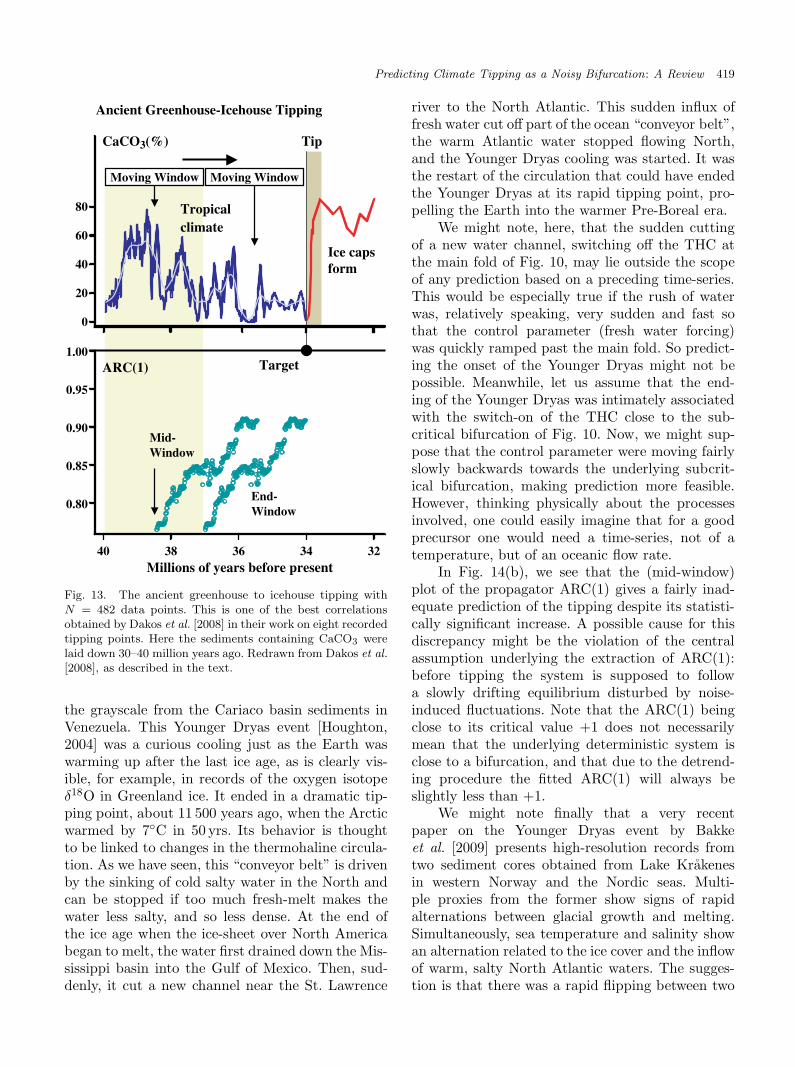
March 10, 2011 11:27 WSPC/S0218-1274 02851


Ancient Greenhouse-Icehouse Tipping

CaCO3(%) Tip

Moving Window Moving Window

80

1.00

0.95

0.85

0.90

0.80

40 38 36 34 32

60

40

20

0

ARC(1) Target

Mid-Window

End-Window

Ice capsform

Tropicalclimate

Millions of years before present

Fig. 13. The ancient greenhouse to icehouse tipping withN = 482 data points. This is one of the best correlationsobtained by Dakos et al. [2008] in their work on eight recordedtipping points. Here the sediments containing CaCO3 werelaid down 30–40 million years ago. Redrawn from Dakos et al.[2008], as described in the text.

the grayscale from the Cariaco basin sediments inVenezuela. This Younger Dryas event [Houghton,2004] was a curious cooling just as the Earth waswarming up after the last ice age, as is clearly vis-ible, for example, in records of the oxygen isotopeδ18O in Greenland ice. It ended in a dramatic tip-ping point, about 11 500 years ago, when the Arcticwarmed by 7◦C in 50 yrs. Its behavior is thoughtto be linked to changes in the thermohaline circula-tion. As we have seen, this “conveyor belt” is drivenby the sinking of cold salty water in the North andcan be stopped if too much fresh-melt makes thewater less salty, and so less dense. At the end ofthe ice age when the ice-sheet over North Americabegan to melt, the water first drained down the Mis-sissippi basin into the Gulf of Mexico. Then, sud-denly, it cut a new channel near the St. Lawrence

river to the North Atlantic. This sudden influx offresh water cut off part of the ocean “conveyor belt”,the warm Atlantic water stopped flowing North,and the Younger Dryas cooling was started. It wasthe restart of the circulation that could have endedthe Younger Dryas at its rapid tipping point, pro-pelling the Earth into the warmer Pre-Boreal era.

We might note, here, that the sudden cuttingof a new water channel, switching off the THC atthe main fold of Fig. 10, may lie outside the scopeof any prediction based on a preceding time-series.This would be especially true if the rush of waterwas, relatively speaking, very sudden and fast sothat the control parameter (fresh water forcing)was quickly ramped past the main fold. So predict-ing the onset of the Younger Dryas might not bepossible. Meanwhile, let us assume that the end-ing of the Younger Dryas was intimately associatedwith the switch-on of the THC close to the sub-critical bifurcation of Fig. 10. Now, we might sup-pose that the control parameter were moving fairlyslowly backwards towards the underlying subcrit-ical bifurcation, making prediction more feasible.However, thinking physically about the processesinvolved, one could easily imagine that for a goodprecursor one would need a time-series, not of atemperature, but of an oceanic flow rate.

In Fig. 14(b), we see that the (mid-window)plot of the propagator ARC(1) gives a fairly inad-equate prediction of the tipping despite its statisti-cally significant increase. A possible cause for thisdiscrepancy might be the violation of the centralassumption underlying the extraction of ARC(1):before tipping the system is supposed to followa slowly drifting equilibrium disturbed by noise-induced fluctuations. Note that the ARC(1) beingclose to its critical value +1 does not necessarilymean that the underlying deterministic system isclose to a bifurcation, and that due to the detrend-ing procedure the fitted ARC(1) will always beslightly less than +1.

We might note finally that a very recentpaper on the Younger Dryas event by Bakkeet al. [2009] presents high-resolution records fromtwo sediment cores obtained from Lake Krakenesin western Norway and the Nordic seas. Multi-ple proxies from the former show signs of rapidalternations between glacial growth and melting.Simultaneously, sea temperature and salinity showan alternation related to the ice cover and the inflowof warm, salty North Atlantic waters. The sugges-tion is that there was a rapid flipping between two

March 10, 2011 11:27 WSPC/S0218-1274 02851


End of Younger Dryas, THC switch-on

170

180

190

Grayscale Tip

YoungerDryas

Pre-Boreal

Moving Window

0.97

12400 12000 11600

0.98

0.99

1.00Target

Years before the present

ARC(1)

Moving Window

Mid-Window

Fig. 14. A second illustration taken from Dakos et al. [2008]for the end of the Younger Dryas event using the grayscalefrom basin sediment in Cariaco, Venezuela. The whole of theabove ARC(1) graph fits in the red circle of Fig. 4.

states before the fast tip at the end of YoungerDryas which created the permanent transition toan interglacial state. This strengthens the suspicionthat the deterministic component of the dynamicsbehind the time-series in Fig. 14(a) is not near aslowly drifting equilibrium. It will be interesting tosee if any useful time-series analyses can be madeof this rapid fluttering action.

8. Concluding Remarks

Our illustrations give a snapshot of very recentresearch showing the current status of predictivestudies. They show that tipping events, correspond-ing mathematically to dangerous bifurcations, posea likely threat to the current state of the climatebecause they cause rapid and irreversible transi-tions. Also, there is evidence that tipping eventshave been the mechanism behind climate transi-tions of the past. Model studies give hope that thesetipping events are predictable using time-seriesanalysis: when applied to real geological data frompast events prediction is often remarkably good butis not always reliable. With today’s and tomorrow’s

vastly improved monitoring, giving times-series thatare both longer (higher N) and much more accu-rate, reliable estimates can be confidently expected.However, if a system has already passed a bifurca-tion point it may be too late to do anything useful,because an irreversible transition might be alreadyunderway.

Techniques from nonlinear dynamical systemsenter the modeling side of climate prediction attwo points. First, in data assimilation, which playsa role in the tuning and updating of models, theassimilated data is often Lagrangian (for example,it might come from drifting floats in the ocean).It turns out that optimal starting positions forthese drifters are determined by stable and unsta-ble manifolds of the vector field of the phase-spaceflow [Kuznetsov et al., 2003]. Second, numericalbifurcation-tracking techniques for large-scale sys-tems have become applicable to realistic large-scaleclimate models [Huisman et al., 2009]. More gen-erally, numerical continuation methods have beendeveloped (for example, LOCA by Salinger et al.[2002]) that are specifically designed for the contin-uation of equilibria of large physical systems. Thesegeneral methods appear to be very promising forthe analysis of tipping points in different types ofdeterministic climate models. These developmentswill permit efficient parameter studies where onecan determine directly how the tipping event inthe model varies when many system parametersare changed simultaneously. This may become par-ticularly useful for extensive scenario studies ingeo-engineering. For example, Dijkstra et al. [2004]demonstrated how bifurcation diagrams can helpto determine which perturbations enable threshold-crossing in the bistable THC system, and Biggset al. [2009] studied how quickly perturbations haveto be reversed to avoid jumping to coexisting attrac-tors in a fisheries model.

Furthermore, subtle microscopic nonlinearities,currently beyond the reach of climate models, mayhave a strong influence on the large spatial scale.For example, Golden [2009] observed that the per-meability of sea ice to brine drainage changes dras-tically (from impermeable to permeable) when thebrine volume fraction increases across the five per-cent mark. This microscopic tipping point may havea large-scale follow-on effect on the salinity of seawater near the arctic, and thus, the THC. Incor-porating microscopic nonlinearities into the macro-scopic picture is a challenge for future modelingefforts.

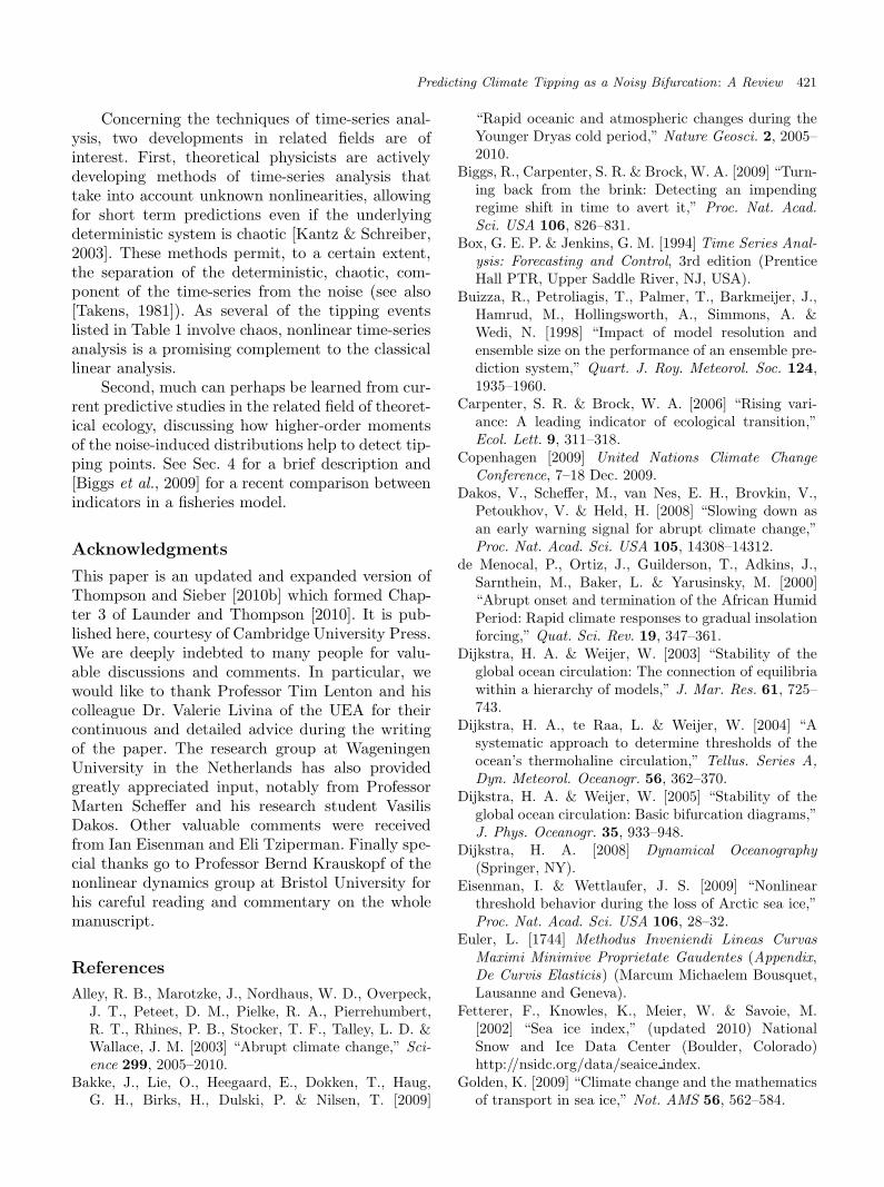
March 10, 2011 11:27 WSPC/S0218-1274 02851


Concerning the techniques of time-series anal-ysis, two developments in related fields are ofinterest. First, theoretical physicists are activelydeveloping methods of time-series analysis thattake into account unknown nonlinearities, allowingfor short term predictions even if the underlyingdeterministic system is chaotic [Kantz & Schreiber,2003]. These methods permit, to a certain extent,the separation of the deterministic, chaotic, com-ponent of the time-series from the noise (see also[Takens, 1981]). As several of the tipping eventslisted in Table 1 involve chaos, nonlinear time-seriesanalysis is a promising complement to the classicallinear analysis.

Second, much can perhaps be learned from cur-rent predictive studies in the related field of theoret-ical ecology, discussing how higher-order momentsof the noise-induced distributions help to detect tip-ping points. See Sec. 4 for a brief description and[Biggs et al., 2009] for a recent comparison betweenindicators in a fisheries model.

Acknowledgments

This paper is an updated and expanded version ofThompson and Sieber [2010b] which formed Chap-ter 3 of Launder and Thompson [2010]. It is pub-lished here, courtesy of Cambridge University Press.We are deeply indebted to many people for valu-able discussions and comments. In particular, wewould like to thank Professor Tim Lenton and hiscolleague Dr. Valerie Livina of the UEA for theircontinuous and detailed advice during the writingof the paper. The research group at WageningenUniversity in the Netherlands has also providedgreatly appreciated input, notably from ProfessorMarten Scheffer and his research student VasilisDakos. Other valuable comments were receivedfrom Ian Eisenman and Eli Tziperman. Finally spe-cial thanks go to Professor Bernd Krauskopf of thenonlinear dynamics group at Bristol University forhis careful reading and commentary on the wholemanuscript.

References

Alley, R. B., Marotzke, J., Nordhaus, W. D., Overpeck,J. T., Peteet, D. M., Pielke, R. A., Pierrehumbert,R. T., Rhines, P. B., Stocker, T. F., Talley, L. D. &Wallace, J. M. [2003] “Abrupt climate change,” Sci-ence 299, 2005–2010.

Bakke, J., Lie, O., Heegaard, E., Dokken, T., Haug,G. H., Birks, H., Dulski, P. & Nilsen, T. [2009]

“Rapid oceanic and atmospheric changes during theYounger Dryas cold period,” Nature Geosci. 2, 2005–2010.

Biggs, R., Carpenter, S. R. & Brock, W. A. [2009] “Turn-ing back from the brink: Detecting an impendingregime shift in time to avert it,” Proc. Nat. Acad.Sci. USA 106, 826–831.

Box, G. E. P. & Jenkins, G. M. [1994] Time Series Anal-ysis: Forecasting and Control, 3rd edition (PrenticeHall PTR, Upper Saddle River, NJ, USA).

Buizza, R., Petroliagis, T., Palmer, T., Barkmeijer, J.,Hamrud, M., Hollingsworth, A., Simmons, A. &Wedi, N. [1998] “Impact of model resolution andensemble size on the performance of an ensemble pre-diction system,” Quart. J. Roy. Meteorol. Soc. 124,1935–1960.

Carpenter, S. R. & Brock, W. A. [2006] “Rising vari-ance: A leading indicator of ecological transition,”Ecol. Lett. 9, 311–318.

Copenhagen [2009] United Nations Climate ChangeConference, 7–18 Dec. 2009.

Dakos, V., Scheffer, M., van Nes, E. H., Brovkin, V.,Petoukhov, V. & Held, H. [2008] “Slowing down asan early warning signal for abrupt climate change,”Proc. Nat. Acad. Sci. USA 105, 14308–14312.

de Menocal, P., Ortiz, J., Guilderson, T., Adkins, J.,Sarnthein, M., Baker, L. & Yarusinsky, M. [2000]“Abrupt onset and termination of the African HumidPeriod: Rapid climate responses to gradual insolationforcing,” Quat. Sci. Rev. 19, 347–361.

Dijkstra, H. A. & Weijer, W. [2003] “Stability of theglobal ocean circulation: The connection of equilibriawithin a hierarchy of models,” J. Mar. Res. 61, 725–743.

Dijkstra, H. A., te Raa, L. & Weijer, W. [2004] “Asystematic approach to determine thresholds of theocean’s thermohaline circulation,” Tellus. Series A,Dyn. Meteorol. Oceanogr. 56, 362–370.

Dijkstra, H. A. & Weijer, W. [2005] “Stability of theglobal ocean circulation: Basic bifurcation diagrams,”J. Phys. Oceanogr. 35, 933–948.

Dijkstra, H. A. [2008] Dynamical Oceanography(Springer, NY).

Eisenman, I. & Wettlaufer, J. S. [2009] “Nonlinearthreshold behavior during the loss of Arctic sea ice,”Proc. Nat. Acad. Sci. USA 106, 28–32.

Euler, L. [1744] Methodus Inveniendi Lineas CurvasMaximi Minimive Proprietate Gaudentes (Appendix,De Curvis Elasticis) (Marcum Michaelem Bousquet,Lausanne and Geneva).

Fetterer, F., Knowles, K., Meier, W. & Savoie, M.[2002] “Sea ice index,” (updated 2010) NationalSnow and Ice Data Center (Boulder, Colorado)http://nsidc.org/data/seaice index.

Golden, K. [2009] “Climate change and the mathematicsof transport in sea ice,” Not. AMS 56, 562–584.

March 10, 2011 11:27 WSPC/S0218-1274 02851


Guilyardi, E. [2006] “El Nino–mean state seasonal cycleinteractions in a multi-model ensemble,” Clim. Dyn.26, 329–348.

Guttal, V. & Jayaprakash, C. [2008a] “Changing skew-ness: An early warning signal of regime shifts inecosystems,” Ecol. Lett. 11, 450–460.

Guttal, V. & Jayaprakash, C. [2008b] “Spatial varianceand spatial skewness: Leading indicators of regimeshifts in spatial ecological systems,” Theoret. Ecol. 2,3–12.

Hansen, J. E. [2005] “A slippery slope: How much globalwarming constitutes ‘dangerous anthropogenic inter-ference’?” Clim. Change 68, 269–279.

Held, H. & Kleinen, T. [2004] “Detection of climatesystem bifurcations by degenerate fingerprinting,”Geophys. Res. Lett. 31, L23207.

Houghton, J. T. [2004] Global Warming: The CompleteBriefing (Cambrige University Press, Cambridge,UK).

Huisman, S. E., Dijkstra, H. A., von Der Heydt, A. &de Ruijter, W. P. M. [2009] “Robustness of multipleequilibria in the global ocean circulation,” Geophys.Res. Lett. 36, L01610.

IPCC [2007] Climate Change 2007, Contribution ofWorking Groups I-III to the Fourth AssessmentReport of the Intergovernmental Panel on Cli-mate Change, I The Physical Science Basis, IIImpacts, Adaptation and Vulnerability, III Mitiga-tion of Climate Change, eds. Solomon, S., Qin, D.,Manning, M., Chen, Z., Marquis, M., Averyt, K. B.,Tignor, M. & Miller, H. L. (Cambridge UniversityPress, Cambridge, UK).

Joos, F., Prentice, I. C., Sitch, S., Meyer, R., Hooss,G., Plattner, G.-K., Gerber, S. & Hasselmann, K.[2001] “Global warming feedbacks on terrestrial car-bon uptake under the intergovernmental panel onclimate change (IPCC) emission scenarios,” Glob.Biogeochem. Cycles 15, 891–907.

Kantz, H. & Schreiber, T. [2003] Nonlinear Time SeriesAnalysis, 2nd edition (Cambridge University Press,Cambridge, UK).

Kleidon, A. & Heimann, M. [2000] “Assessing the roleof deep rooted vegetation in the climate system withmodel simulations: Mechanism, comparison to obser-vations and implications for Amazonian deforesta-tion,” Clim. Dyn. 16, 183–199.

Kleinen, T., Held, H. & Petschel-Held, G. [2003]“The potential role of spectral properties in detect-ing thresholds in the Earth system: Applicationto the thermohaline circulation,” Ocean Dyn. 53,53–63.

Kuznetsov, L., Ide, K. & Jones, C. K. R. T. [2003] “Amethod for assimilation of Lagrangian data,” MonthlyWeather Rev. 131, 2247–2260.

Launder, B. & Thompson, J. M. T. (eds.) [2010]Geo-Engineering Climate Change: Environmental

Necessity or Pandora’s Box? (Cambridge UniversityPress, Cambridge, UK).

Lenton, T. M., Held, H., Kriegler, E., Hall, J. W., Lucht,W., Rahmstorf, S. & Schellnhuber, H. J. [2008] “Tip-ping elements in the Earth’s climate system,” Proc.Nat. Acad. Sci. USA 105, 1786–1793.

Lenton, T. M., Myerscough, R. J., Marsh, R., Livina,V. N., Price, A. R., Cox, S. J. & the GENIE Team[2009] “Using GENIE to study a tipping point in theclimate system,” Philos. Trans. Series A, Math. Phys.Engin. Sci. 367, 871–884.

Lindsay, R. W. & Zhang, J. [2005] “The thinning ofArctic sea ice, 1988–2003: Have we passed a tippingpoint?” J. Climate 18, 4879–4894.

Livina, V. N. & Lenton, T. M. [2007] “A mod-ified method for detecting incipient bifurcationsin a dynamical system,” Geophys. Res. Lett. 34,L03712.

Lockwood, J. [2001] “Abrupt and sudden climatic transi-tions and fluctuations: A review,” Int. J. Climat. 21,1153–1179.

Lorenz, E. N. [1963] “Deterministic nonperiodic flow,”J. Atmosph. Sci. 20, 130–141.

Lucht, W., Schaphoff, S., Erbrecht, T., Heyder, U. &Cramer, W. [2006] “Terrestrial vegetation redistribu-tion and carbon balance under climate change,” Car-bon Balance and Management 1, 6.

McDonald, S. W., Grebogi, C., Ott, E. & Yorke, J. A.[1985] “Fractal basin boundaries,” Physica D: Nonlin.Phen. 17, 125–153.

Morales Maqueda, M. A., Willmott, A. J., Bamber,J. L. & Darby, M. S. [1998] “An investigation of thesmall ice cap instability in the Southern Hemispherewith a coupled atmosphere-sea ice-ocean-terrestrialice model,” Clim. Dyn. 14, 329–352.

National Research Council [2002] Abrupt ClimateChange: Inevitable Surprises (Natl Acad Press, Wash-ington, DC).

Peng, C.-K., Buldyrev, S. V., Havlin, S., Simons, M.,Stanley, H. E. & Goldberger, A. L. [1994] “Mosaicorganization of DNA nucleotides,” Phys. Rev. E 49,1685–1689.

Petit, J. R., Jouzel, J., Raynaud, D., Barkov, N. I.,Barnola, J.-M., Basile, I., Bender, M., Chappellaz, J.,Davis, M., Delaygue, G., Delmotte, M., Kotlyakov,V. M., Legrand, M., Lipenkov, V. Y., Lorius, C.,Pepin, L., Ritz, C., Saltzman, E. & Stievenard, M.[1999] “Climate and atmospheric history of the past420,000 years from the Vostok ice core, Antarctica,”Nature 399, 429–436.

Petoukhov, V., Ganopolski, A., Brovkin, V., Claussen,M., Eliseev, A., Kubatzki, C. & Rahmstorf, S. [2000]“CLIMBER-2: A climate system model of inter-mediate complexity. Part I: Model description andperformance for present climate,” Clim. Dyn. 16,1–17.

March 10, 2011 11:27 WSPC/S0218-1274 02851


Poincare, H. [1885] “Sur l’equilibre d’une masse fluideanimee d’un mouvement de rotation,” Acta Mathe-matica 7, 259–380.

Poston, T. & Stewart, I. [1978] Catastrophe Theory andits Applications (Pitman, London, UK).

Rahmstorf, S. [2000] “The thermohaline ocean circu-lation: A system with dangerous thresholds?” Clim.Change 46, 247–256.

Rahmstorf, S. [2001] “Abrupt climate change,” Ency-clopaedia of Ocean Sciences, eds. Steele, J.,Thorpe, S. & Turekian, K. (Academic Press, London),pp. 1–6.

Rahmstorf, S. [2002] “Ocean circulation and climate dur-ing the past 120 000 years,” Nature 419, 207–214.

Rahmstorf, S., Crucifix, M., Ganopolski, A., Goosse, H.,Kamenkovich, I., Knutti, R., Lohmann, G., Marsh,R., Mysak, L. A., Wang, Z. & Weaver, A. J. [2005]“Thermohaline circulation hysteresis: A model inter-comparison,” Geophys. Res. Lett. 32, L23605.

Rial, J. A., Pielke, R. A., Beniston, M., Claussen,M., Canadell, J., Cox, P., Held, H., de Noblet-Ducoudre, N., Prinn, R., Reynolds, J. F. & Salas,J. D. [2004] “Nonlinearities, feedbacks and criticalthresholds within the Earth’s climate system,” Clim.Change 65, 11–38.

Salinger, A. G., Bou-Rabee, N. M., Pawlowski, R. P.,Wilkes, E. D., Burroughs, E. A., Lehoucq, R. B. &Romero, L. A. [2002] “LOCA 1.0 Library of contin-uation algorithms: Theory and implementation man-ual,” Sandia National Laboratories, SAND2002-0396.

Saltzman, B. [2002] Dynamical Paleoclimatology (Aca-demic Press, London, UK).

Scheffer, M. [2009] Critical Transitions in Nature andSociety (Princeton University Press, Princeton, USA).

Selten, F. M., Branstator, G. W., Dijkstra, H. A. &Kliphuis, M. [2004] “Tropical origins for recent andfuture Northern Hemisphere climate change,” Geo-phys. Res. Lett. 31, L21205.

Sperber, K. R., Brankovic, C., Deque, M., Frederik-sen, C. S., Graham, R., Kitoh, A., Kobayashi, C.,Palmer, T., Puri, K., Tennant, W. & Volodin, E.[2001] “Dynamical seasonal predictability of the Asiansummer monsoon,” Monthly Weather Rev. 129, 2226–2248.

Stommel, H. [1961] “Thermohaline convection with twostable regimes of flow,” Tellus 13, 224–230.

Takens, F. [1981] “Detecting strange attractors in tur-bulence,” Dynamical Systems and Turbulence, eds.Rand, D. A. & Young, L. S. (Springer, Berlin & NY),Chapter 21, pp. 366–381.

Thompson, J. M. T. & Hunt, G. W. [1973] A GeneralTheory of Elastic Stability (Wiley, London).

Thompson, J. M. T. [1982] Instabilities and Catastrophesin Science and Engineering (Wiley, Chichester, UK).

Thompson, J. M. T. & Hunt, G. W. [1984] Elastic Insta-bility Phenomena (Wiley, Chichester, UK).

Thompson, J. M. T. [1992] “Global unpredictability innonlinear dynamics: Capture, dispersal and the inde-terminate bifurcations,” Physica D: Nonlin. Phen. 58,260–272.

Thompson, J. M. T., Stewart, H. B. & Ueda, Y. [1994]“Safe, explosive, and dangerous bifurcations in dissi-pative dynamical systems,” Phys. Rev. E 49, 1019–1027.

Thompson, J. M. T. [1996] “Danger of unpredictable fail-ure due to indeterminate bifurcation,” Zeitschrift furangewandte Mathematik und Mechanik 76, 205–208.

Thompson, J. M. T. & Stewart, H. B. [2002] NonlinearDynamics and Chaos, 2nd edition (Wiley, Chichester,UK).

Thompson, J. M. T. & Sieber, J. [2010] “Predict-ing climate tipping points,” Geo-Engineering ClimateChange: Environmental Necessity or Pandora’s Box?,eds. Launder, B. & Thompson, J. M. T. (CambridgeUniversity Press, Cambridge, UK), Chapter 3,pp. 50–83.

Thompson, J. M. T. & Sieber, J. [2011] “Climate tippingas a noisy bifurcation: A predictive technique,” IMAJ. Appl. Math. 76, 27–46.

Timmermann, A., Oberhuber, J., Bacher, A., Esch, M.,Latif, M. & Roeckner, E. [1999] “Increased El Ninofrequency in a climate model forced by future green-house warming,” Nature 398, 694–697.

Tziperman, E., Toggweiler, J. R., Bryan, K. & Feliks,Y. [1994] “Instability of the thermohaline circulationwith respect to mixed boundary conditions: Is it reallya problem for realistic models?” J. Phys. Oceanogr.24, 217–232.

Tziperman, E. [1997] “Inherently unstable climatebehavior due to weak thermohaline ocean circula-tion,” Nature 386, 592–595.

van Nes, E. H. & Scheffer, M. [2007] “Slow recovery fromperturbations as a generic indicator of a nearby catas-trophic shift,” The American Naturalist 169, 738–747.

Winton, M. [2006] “Does the Arctic sea ice have a tippingpoint?” Geophys. Res. Lett. 33, L23504.

Zeng, N., Dickinson, R. E. & Zeng, X. [1996] “Cli-matic impact of Amazon deforestation — a mecha-nistic model study,” J. Clim. 9, 859–883.

Zickfeld, K., Knopf, B., Petoukhov, V. & Schellnhuber,H. J. [2005] “Is the Indian summer monsoon sta-ble against global change?” Geophys. Res. Lett. 32,L15707.

PREDICTING CLIMATE TIPPING AS A NOISY BIFURCATION: A …

Documents

Transcript of PREDICTING CLIMATE TIPPING AS A NOISY BIFURCATION: A …