LLNL-TR-737609

Precision and Accuracy in PDVand VISAR

W. P. Ambrose

August 28, 2017

Disclaimer

This document was prepared as an account of work sponsored by an agency of the United States government. Neither the United States government nor Lawrence Livermore National Security, LLC, nor any of their employees makes any warranty, expressed or implied, or assumes any legal liability or responsibility for the accuracy, completeness, or usefulness of any information, apparatus, product, or process disclosed, or represents that its use would not infringe privately owned rights. Reference herein to any specific commercial product, process, or service by trade name, trademark, manufacturer, or otherwise does not necessarily constitute or imply its endorsement, recommendation, or favoring by the United States government or Lawrence Livermore National Security, LLC. The views and opinions of authors expressed herein do not necessarily state or reflect those of the United States government or Lawrence Livermore National Security, LLC, and shall not be used for advertising or product endorsement purposes.

This work performed under the auspices of the U.S. Department of Energy by Lawrence Livermore National Laboratory under Contract DE-AC52-07NA27344.

1

Precision and accuracy in PDV and VISAR

W. P. Ambrose

Aug. 21, 2017

Abstract

This is a technical report discussing our current level of understanding of a wide and varying distribution

of uncertainties in velocity results from Photonic Doppler Velocimetry in its application to gas gun

experiments. Using propagation of errors methods with statistical averaging of photon number

fluctuation in the detected photocurrent and subsequent addition of electronic recording noise, we

learn that the velocity uncertainty in VISAR can be written in closed form. For PDV, the non-linear

frequency transform and peak fitting methods employed make propagation of errors estimates

notoriously more difficult to write down in closed form expect in the limit of constant velocity and low

time resolution (large analysis-window width). An alternative method of error propagation in PDV is to

use Monte Carlo methods with a simulation of the time domain signal based on results from the spectral

domain. A key problem for Monte Carlo estimation for an experiment is a correct estimate of that

portion of the time-domain noise associated with the peak-fitting region-of-interesting in the spectral

domain. Using short-time Fourier transformation spectral analysis and working with the phase

dependent real and imaginary parts allows removal of amplitude-noise cross terms that invariably show

up when working with correlation-based methods or FFT power spectra. Estimation of the noise

associated with a given spectral region of interest is then possible. At this level of progress, we learn

that Monte Carlo trials with random recording noise and initial (uncontrolled) phase yields velocity

uncertainties that are not as large as those observed. In a search for additional noise sources, a speckle-

interference modulation contribution with off axis rays was investigated, and was found to add a

velocity variation beyond that from the recording noise (due to random interference between off axis

rays), but in our experiments the speckle modulation precision was not as important as the recording

noise precision. But from these investigations we do appreciate that the velocity-uncertainty itself has a

wide distribution of values that varies with signal-amplitude modulation (is not a single value). To

provide a rough rule of thumb for the velocity uncertainty, we computed the average of the relative

standard deviation distributions from 60 recorded traces (with distributions of uncertainties roughly

between 0.1 % to 1 % in each trace) and found a mean of the distribution of uncertainties for our

experiments is not better than 0.4 % at an analysis window width of 5 ns (although for brief intervals it

can be as good as 0.1 %). Further imagination and testing may be needed to reveal other possible

hydrodynamics-related sources of velocity error in PDV.

2

Introduction

Precision and accuracy are best understood as the standard deviation and difference of the mean of

results from an “expected” result for a large ensemble of identically-prepared experiments. Propagation

of uncertainty estimates may be used to estimate precision when an ensemble of identical experiments

is not available. Propagation of error methods also allow tests of insights into the relative importance of

possible error sources.

For example, one may test how velocity precision depends on signal-to-noise ratios in digital-signal

recordings. Propagation-of-errors methods applied under a limited set of conditions (constant velocity,

low demands on time resolution, small noise and large optical power) reveal that velocity precision is

directly proportional to noise-to-signal ratio for both VISAR and PDV (when no other error sources are

expected).

Often it is possible to make a distinction between small rapid amplitude noise and much stronger (and

slower) amplitude variations of other types. The signal amplitude may vary due to speckle interference,

polarization modulation, additional background light, and variation in optical collection efficiency as the

target surface moves. This leads to a simple but important concept to keep in mind – the precision is

not a constant value and itself has a wide distribution of values. In other words, when using optical

velocimetry there may be practical difficulties that lead to a lack of full control over creation of

ensembles of identical experiments.

Another method for estimating precision shares elements of the propagation-of-errors method and the

direct calculation of precision in an ensemble of identical experiments – the Monte Carlo method.

Monte Carlo methods have an added advantage that they are only limited by a physical theory for the

system, theory of measurement, adequacy of the simulation inputs and assumed noise sources (may be

more generally applicable than approximations based on small noise, constant velocity, etc.). Even

more importantly, Monte Carlo methods can use the same numerical methods used in the analysis of

experimental data. It is comforting that results of Monte Carlo statistics agree with qualitative results

for the algebraic propagation-of-errors estimates with the same dependencies on noise, amplitude, and

time resolution. But the Monte Carlo methods are not hampered by incomplete knowledge of the

instrument impulse responses for all stages of detection and recording, for example.

In an experiment where we expect a constant velocity with time, the uncertainties in PDV appear to vary

strongly from one measurement to the next and across an ensemble at one time with precision typically

between 0.1 and 1 % depending on the noise-to-amplitude ratio, and the time resolution set by the

width of an analysis-time window. PDV analysis has a built in “smoothing” effect by the analysis window

used to set the time resolution, with velocity precision improving as the -3/2 power of the window width

(3/2~ 1/ w ). Where the amplitude is low, it may be possible to buy back precision by giving up time

resolution. If one wishes to sacrifice, say, a factor of 5 in time resolution, one may gain back more than

a factor of 10 in precision. This is an interesting effect for anyone accustomed to precision improving

only as the square root of the number of measurements – as is the case for VISAR.

In the following, we explore also the less obvious possibility that summation over different optical paths

in three dimensions combined with speckle interference effects may create velocity accuracy errors. We

use a numerical model with random surface roughness and electrodynamics in three dimensions to

examine whether there is a connection between speckle amplitude modulation and velocity errors, and

3

find that this is another source of inverse correlation between signal amplitude and velocity error. For

the limited set of conditions explored so far, speckle-interference modulation in JASPER targets is not

larger than 0.2 % and not larger than the noise-to-amplitude precision at 2 ns time resolution.

Propagation of errors estimation and Monte Carlo precision estimation

Signals and target metrology values iX X are combined to create a desired result f X (e.g., the

mass velocity). By expanding f X in iX X for small random error estimates idX , computing

the variance 2

f , assuming uncorrelated precision estimates Xi and performing large-ensemble

averaging, the variances are related through rates of change of f X through

22 2/f i XiXi

f X .

For a four-port VISAR, an explicit function f X and its derivatives / if X are possible (see below).

For the usual implementation of PDV (one interferometer port) with peak fitting in the spectral domain,

the apparent velocity is not available as an explicit function f X , but is determined implicitly through

numerical estimation. Precision estimates by propagation of errors methods are still possible for PDV

under limited conditions where we may extract explicit (but approximate) expressions for the

derivatives / if X .

When the luxury of repeating actual experiments is not available, an alternative method for precision

estimation is statistical estimation using simulated measurements and results analysis – this is the

Monte Carlo method. Monte Carlo methods require some underlying physical theory to generate the

signals iX X , to which we add directly random estimates idX pulled from appropriate

distributions for the uncontrolled parts of the experiment (e.g., noise). Monte Carlo methods have the

distinct advantage that they need not be limited to specific conditions needed to write down derivatives

/ if X and the variance 22 2/f i XiXi

f X , and may include the same numerical methods to

estimate the results f X from an “experiment.”

Theory of measurement for PDV and VISAR -- aspects in common to both

A laser field reflected from a moving target surface is collected and returned with a Doppler frequency

shift compared to the laser source. In the usual one-dimensional approximation, the Doppler frequency

difference

2( / ) 2( / )D LASER LASER LASERf f f V c f V

is proportional to the component of the reflecting-surface velocity V along the optical path direction.

(for technical reasons beyond the scope of this discussion, VISAR is often operated at visible-green

4

wavelengths of 514 or 532 nm, and PDV is operated in the near infrared most often near 1550 nm).

VISAR and PDV are interferometric techniques for measuring small changes in optical wavelength or

frequency. In VISAR, a Doppler-shifted optical signal is injected into an interferometer with fixed but

different path lengths. In PDV, the moving target surface is included as one of the mirrors in an

interferometer (PDV). An alternative description of PDV is that heterodyne mixing with a reference field

at a detector creates an beat frequency to appear in the optical power at the Doppler shift frequency.

A tamping window is used in situations where it is not known in advance if the surface will stop

reflecting due to, e.g., a loss of material strength. In a classical picture, the Doppler shift can be

understood as arising from an advance in the optical field phase (relative to a reference) due to changes

in the optical path length as the reflecting surface moves. The optical path length has two contributions.

The path length variation includes not only the moving surface contribution, but includes also a

contribution by a growing thickness of compressed window material with different index of refraction.

The measured velocity is an apparent velocity that needs correction by a velocity correction function (In

PDV and VISAR, the simplest first order approximation is to divide the apparent velocity by

approximately 1.27, which has an error of approximately 1 % at several kilometers per second). In

recent years, improvements in velocity correction methods have reduced the accuracy error to as low as

0.1 % in the range of several kilometers per second using a power law correction and covariance matrix

to describe the errors in two correction-function parameters. [Rigg et. al 2014]

In the following, we will discuss error propagation for apparent velocities. We begin by showing results

from analytical methods for continuous functions and evolve this to Monte Carlo simulations of digitally

sampled data to gain insights into the effects of signal and an obvious error source, noise, in recorded

data.

Theory of measurement and error propagation for VISAR

For general interest, we include here a closed form solution for precision in VISAR. The interesting part

of this discussion appears when we compare the similarities and differences from the PDV case. In

VISAR, four optical power levels are measured at the two outputs of an interferometer in two

polarizations. For a carefully balanced system with appropriate phase delays in the two polarizations,

the four optical power levels can be arranged to have this functional relationship:

P1 Po Ps cos

P2 Po Ps cos

P3 Po Ps sin

P4 Po Ps sin

The VISAR interference contrast sP rides on a background oP (note that when we write these two

power levels for either PDV or VISAR we mean always that the signal s oP P is less than the average or

background value). The interference phase depends on fixed path lengths and wavelength, and is

linear with velocity (has constant value at constant velocity). VISAR depends on the use of linear

detectors with similar gain values converting optical power to signal voltages iV . Subtraction and

5

division of recorded signals removes common backgrounds and common amplitude modulation allowing

us to isolate the tangent of the interference phase:

tan12

34

VV

VVF

This form is directly amenable to the method of propagation of errors by derivatives. After some work

including ensemble averaging of photon-impulse responses with Poisson statistics for photon shot noise,

one-standard deviation uncertainty (precision) in the apparent velocity for VISAR can be written

1/22

1/2

3 2

1 1 1 1 12

2 2 2 2

n

VISAR

VoV r

sv v d

hH H P H

t G P

The proportionality between the phase noise and velocity noise includes a “velocity per fringe” constant

/ 2 v where is optical wavelength and v is an interferometer delay time. The expression inside

the curly brackets is the sum of variances of the two noise sources, recorder noise and photon shot

noise. The velocity precision is proportional to the ratio of a “noise-power” (proportional to the square

root of the expression in curly brackets) to the signal power sP . Operationally one may observe the

following. When the light is turned off, 0oP , we see the electronics noise nV (referenced back to

the detector by dividing by the total system gain G ). When the light is on, one may then observe

additional noise at high frequencies due to the detected-photon shot noise variance proportional to the

number of detected photons in detector response time dt after detecting optical power with quantum

efficiency . When shot noise is measurable (which happens when we are required to have small

detector response time dt or limited optical power on the target compensated with larger electronic

gainG ), improvements are obtained not only with larger signal at the recorder, but also with larger

optical contrast s oP P . The noise variances are modified by impulse shapes and bandwidth limits at

various stages of the detection and recording system. Dimensionless factors and iH are of order

unity and are related to convolution integrals involving photon-impulse response functions.

Propagation of errors in PDV in the continuous-function approximation

In PDV, coherent interference of reference power refP and surface-reflected power surfP creates an

oscillatory optical power from one port of an un-polarized interferometer at a detector with an

expression of the form

cos cosref surf ref surf o sP P P C P P P P .

For comparison with VISAR we convert this to an expression with background oP and signal power sP .

Unlike VISAR, the phase difference is accumulated at a rate given by the Doppler shift frequency

difference D t :

6

' 't

Ddt t

This phase is unlike the VISAR interferometer phase, as it advances linearly in time for constant nonzero

Doppler shift D t . The constant of integration o (established while the surface is not moving and

with 0D ) depends on the optical path difference between reference and surface reflections

(initially fixed but not normally controlled). For constant velocity, a high-frequency signal modulation

takes the form ~ cosref surf D oC P P t . The signal contrast factorC in the first PDV expression

depends on polarization alignment at the detector (not normally controlled). The power returned from

the moving surface surfP is affected by speckle-interference modulation and optical collection efficiency

variations as the surface moves (also random and usually slower than the oscillations ~ cos D ot ).

To introduce time resolution, a multiplicative window function w t peaked at 0t and falling to zero

for some window width / 2wt is selected to restrict the time range. At each time ot , a suitable

frequency transform oS FT w t t V t is examined searching for a peak D ot separated

from the modulation spectra belonging to surfP and C . Numerical methods for extracting a value for

the peak D ot include non-linear least squares iterative minimization of the sum of squares of

differences between the power spectrum S S

and a peaked fitting function W W

in a

selected region of interest (ROI), e.g., by minimization of a function such as

2

2 ~ o o

ROI

d S S W W

,

where the peak position o converges on D ot near a minimum in 2 . Iterative minimization is

algebraically equivalent to setting derivatives such as 2 / 0D . Progress towards obtaining

additional derivatives of D ot needed for propagation of errors estimation derived from within the

2 / 0D expression can be obtained using an expansion in small noise at constant velocity. The

integrals that appear do not have known solutions, in general. By numerical estimation of these

integrals, one is at first surprised to find that there are terms in the precision for D that oscillate and

decay away with increasing window widths that are a few times wider than a couple of Doppler cycles,

4 /w D . For wide enough window width, constant velocity and small noise values, an

approximate solution may be found for the remaining term (the one that does not decay). Under these

limited conditions, a result for the uncertainty in the apparent velocity in PDV becomes

1/221/2

1

1 1 1

2 2

n

PDV

VoV r

sw w d

hH P H

t G P

7

This form has similarities to the expression from propagation of errors in the VISAR case shown above

(see above for additional description of factors). There is a different factor (instead of 1/2

3H ) of order

a factor of “a few” related to a convolution integral of the window function w t . Due to an effective of

temporal smoothing by the window function width w , the fixed interferometer delay v in VISAR is

replaced by a factor3/2

w in the denominator for PDV that may be adjusted after an experiment. As with

VISAR, the overall form for the precision in PDV is a proportionality to the recording noise-to-signal

ratio, with the noise having variance contributions from electronic noise and photon detection shot

noise. VISAR may have a slight advantage over PDV when short-time resolution is required (PDV

performs poorly when the demands on time resolution requires 2 /w D , and performs

exceptionally poorly when the duration of a wave such as a low velocity elastic precursor is less than

/ D ). PDV may always have an advantage over VISAR after an experiment is performed at high

velocities when time resolution can be set arbitrarily longer than v . Notice the feature common to PDV

and VISAR that the precision contribution from recorded signal and noise considerations alone is directly

proportional to the noise-to-amplitude ratio in the recorded signals.

Monte Carlo precision estimation in PDV for simulated digitally-sampled data

Dolan [Dolan 2010] used Monte Carlo estimation methods to simulate digitally sampled data and

demonstrated clearly the oscillatory contribution to the uncertainty when the number of “PDV fringes”

per window width was small, with the oscillation damping down for wide windows. Dolan found by

Monte Carlo simulation and numerical estimation that the limiting precision in the peak frequency for

wide windows at constant velocity can be approximated by

1/2

1/2 3/2

6 1 1 noisef

s wf A

Here, the combined total noise in the voltage recording is noise and the oscillatory signal amplitude is

A . For comparison, the noise-to-signal ratio /noise A is analogous to the expression above in the

continuous case with

1/22

1/ ~ /nVo snoise r

d

hA H P H P

t G

.

For simulation purposes Dolan set “a noise level” without distinguishing between optical and electronic

noise. The same factor of 3/2

w for the window width appears in the continuous case and simulated

digitally sampled cases. Because Dolan had performed his Monte Carlo analysis on simulated digital

records sampled at a recording sample rate of sf , he found also the useful observation that when using

digital sampling the precision improves with sample rate as 1/21/ sf . In other words, one should always

sample at the highest available sample rate in the digital recorder. In digital recordings at high speed,

8

the signal to noise ratio is rarely large as 256, but can be as large as 100 (for large signal amplitude).

These expressions suggest the limiting relative precision in velocity for wide window widths can be

better than 0.1 % under good conditions of constant velocity in the range of several kilometers per

second and large signal amplitudes A with SNR of order 100.

Monte Carlo simulation of experimental results

Rather than piecemeal trying to include enough error sources and other factors needed in the precision

estimate (i.e., convolution integrals , , or the iH ), we now pursue an obvious natural extension of

the Monte Carlo approach. Simulating data and applying PDV analysis methods to the simulation results

is not restricted to small noise, constant velocities, and wide analysis windows. Instead for the

simulation we use interpolated results of an analysis of “real” data with time varying amplitude and non-

linear phase advance. For the bundled value noise in the time domain we compare the residuals to the

fit in the spectral domain to find a standard deviation noise in the time domain that produces the same

result in the fit-region-of-interest. For the phase in the simulation, we use results from the experiment

analysis for D it with interpolation onto the sample interval in an experiment recording, and compute

trapezoid-like replacement for the nth point of the time varying phase after shock breakout similar to

1' ' / 2breakout nt

n D o D i D i

i breakout

dt t t t t

.

For the Monte Carlo trials, we vary the noise (pulled from a Gaussian distribution), and initial phase

value (uniformly distributed on 2 ). The same analysis methods used to extract results from an

experiment recording are then applied to the simulated trials with Monte Carlo variations (FT transform

with a window and peak fitting).

Following this method, we expect that the signal amplitude and amplitude-to-noise variations in data

should be reflected in the precision in the results. The advantage of this method, in addition to

increased generality to velocities and amplitudes that are not constant, is the use of the actual analysis

algorithm used to extract results from the experiment, and that it does not depend on expressions

requiring a correct proportionality constant between the noise-to-amplitude ratio and the velocity

precision (do not need to know the variance modifying convolution integrals , , or the iH ). On the

other hand, note that the method assumes no other error sources than recording noise and

uncontrolled initial phase.

We applied this method to results from flat plate target spiral-1 shot in JAS131. The impactor had a

thick front end of magnesium. The target has 0.3 mm of aluminum backed by a thick LiF window (with

glue layer). We expect reverberations in the aluminum and glue to settle down before 50 ns after

impact, and we can expect the velocity should be constant between 50 and 150 ns. For an apparent

velocity near 2 km/sec, the PDV signal oscillates near 1.5 GHz. For this work, a Gaussian analysis

window width was set at a somewhat demanding value of 2 ns full width at half maximum

(approximately 3 oscillations per window).

9

Figure 1 shows a mass velocity trace for a GDI surrogate shot JAS131, and two traces at plus and minus

one standard deviation in the velocity as determined by the Monte Carlo estimation process. With at

time resolution near 2 ns, the mass velocity has moment-to-moment variations on the order of 1

percent. These velocity variations easily can be reduced when using a window widthw wider than 2 ns.

Figure 1. Mass velocity results from Spiral-1 JAS131 with plus-and-minus Monte Carlo precision.

In Figure 1, the results of Monte Carlo precision are shown also as plus and minus one standard

deviation around the experimental trace. As can be seen in the Figure, the precision from Monte Carlo

estimation does vary from point to point, but by an amount that is not as large as actual velocity

variations. All thirteen traces in JAS131 showed similar levels of actual variation and smaller Monte

Carlo derived precision. Ensemble overlays of thirteen channels also imply a large variation on the order

of 1 % at 2 ns resolution.

Electrodynamics simulation of speckle interference amplitude modulation in three dimensions

Apparently, the random noise, uncontrolled initial phase, and modest analysis window width are not

enough to account for the observed precision. Amplitude modulation in the signal is in part due to

surface roughness added to the LiF with average absolute value in the roughness of 0.15 to 0.2 microns

to desensitize the PDV amplitudes to impactor tilt up to 3 degrees. From electrodynamics modelling in

three-dimension [Ambrose 2015, LLNL-TR-677076], we became aware that different optical paths

combined with speckle interference results in small velocity accuracy errors. Figure 2 depicts the

geometry of PDV with a fiber optic probe and collection lens.

10

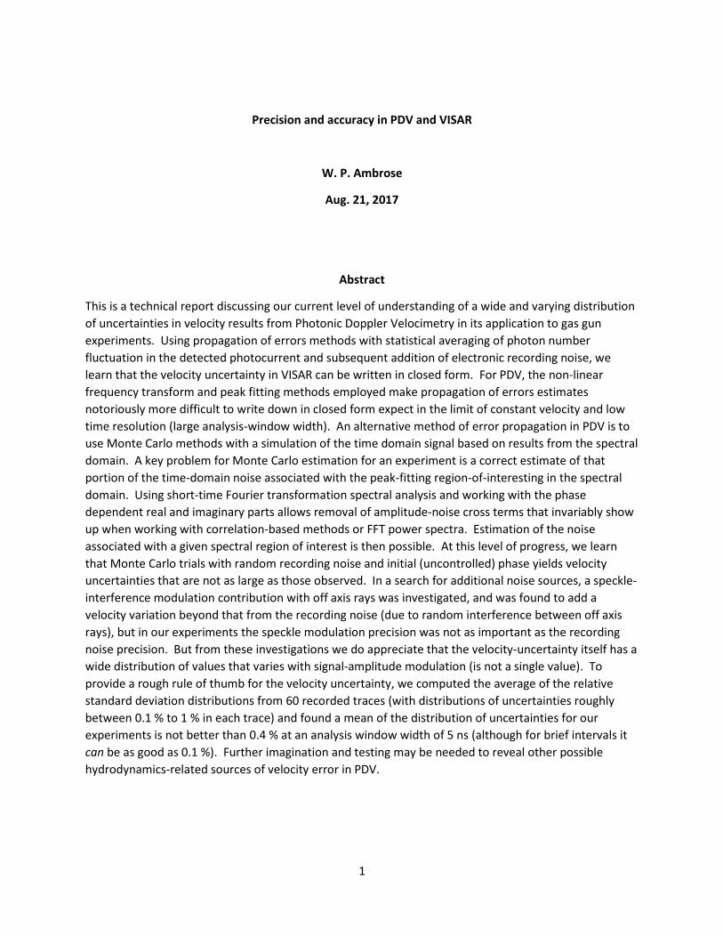
Figure 2. Geometry for electrodynamics simulations of PDV in three dimensions.

Light scattered from target points ir passes through lens aperture points ar , and arrives at an optical

fiber at P along different directions a ir r . Fields at P contribute different frequencies containing

information about the components of the velocity along these different directions a ir r . In the

absence of roughness, the accuracy error introduced by wave front curvature alone can be on the order

of 0.05 %. With roughness, random phase interference in the field summation can create a larger

accuracy error. We performed an analysis of the statistics of speckle interference effects in three

dimensions. For an experiment like the one in Fig. 1, a Monte Carlo statistical analysis of speckle

interference effects leads to a connection between velocity precision and the signal amplitude shown in

Fig. 3.

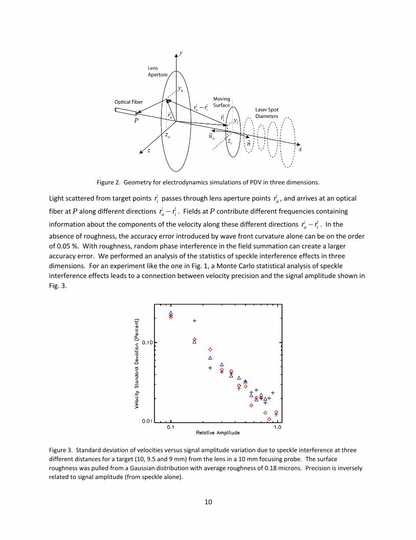
Figure 3. Standard deviation of velocities versus signal amplitude variation due to speckle interference at three

different distances for a target (10, 9.5 and 9 mm) from the lens in a 10 mm focusing probe. The surface

roughness was pulled from a Gaussian distribution with average roughness of 0.18 microns. Precision is inversely

related to signal amplitude (from speckle alone).

11

Signal to noise ratio in a recording leads to precision directly proportional to noise-to-signal ratio (when

only the recording noise is considered). In the absence of recording noise in a continuous

electrodynamics simulation, we find that speckle interference induced velocity errors also have an

inverse correlation to signal amplitude.

Further work may be needed to discover additional sources of velocity error

Accuracy in PDV is probably no worse than ~ 0.1 % in the range of a few kilometers per second (mainly

due to window correction factor errors, but also due to optical wave front curvature effects). Signal

amplitudes vary for a variety of reasons. Random sources (recording noise and speckle interference

amplitude modulation) each contribute to the precision in PDV that varies inversely with the signal

amplitude. With a somewhat challenging time resolution of w = 2 ns used in the analysis in Fig. 1, the

precision appears to vary between 0.1 and 1 %. The precision can be improved faster than linear with a

somewhat less demanding time resolution value by the factor of 3/2

w in the denominator of the PDV

precision expressions shown above. We examined the average of the relative standard deviations of the

velocity distributions from 60 recorded traces (with a variety of different but constant velocities). Using

a wider analysis window width of 5 ns (instead of 2 ns) gave an average of the relative standard

deviation distributions no better than 0.4 %. Speckle interference effects, amplitude variations, and

recording noise used as inputs to Monte Carlo precision estimates does account fully for the size of the

velocity variations in Figure 1.

Imagination and testing are needed to discover other possible sources of error. Another possible source

of velocity error (unconfirmed) is a shock front in the window with small pressure variations in the LiF

window caused by the window surface roughness leading to inhomogeneous velocity correction effects.

Or there may be small density variations in the impactor or glue layers (also unconfirmed). To confirm

these hypotheses would require additional numerical modeling and experimental testing.

Acknowledgements

The author would like to thank Minta Akin, Ricky Chau, Neil Holmes, Jeff Nguyen, Tom Arsenlis and

Dennis McNabb for reading this summary and providing comments.

Bibliography

[Ambrose 2015] W. P. Ambrose, “Photonic-Doppler-Velocimetry, Paraxial-Scalar Diffraction Theory and

Simulation,” Lawrence Livermore National Laboratory Technical Report number LLNL-TR-677076 (2015).

[Dolan 2010] D. H. Dolan, “Accuracy and precision in photonic Doppler velocimetry,” Review of Scientific

Instruments, Vol 81, 053905 (2010).

12

[Rigg 2014] P. A. Rigg, M. D. Knudson, R. J. Scharff, and R. S. Hixon, “Determining the refractive index of

shocked [100] lithium fluoride to the limit of transmissibility,” J. Appl. Phys., Vol. 116, 033515 (2014).