Lawrence Livermore National Laboratory

Lawrence Livermore National Laboratory, P. O. Box 808, Livermore, CA 94551

This work performed under the auspices of the U.S. Department of Energy by Lawrence Livermore National Laboratory under Contract DE-AC52-07NA27344

Damon D Jackson

PDV Analysis using Igor Pro

UCRL-PRES-233496

Lawrence Livermore National Laboratory

Igor Pro

According to the WaveMetrics web page:• Igor Pro is an extraordinarily powerful and extensible

scientific graphing, data analysis, image processing and programming software tool for scientists and engineers.

Runs on both a Mac and PC Both command line and/or menu driven Great for:

• Data Analysis• Loading huge files• Automating common procedures

Lawrence Livermore National Laboratory

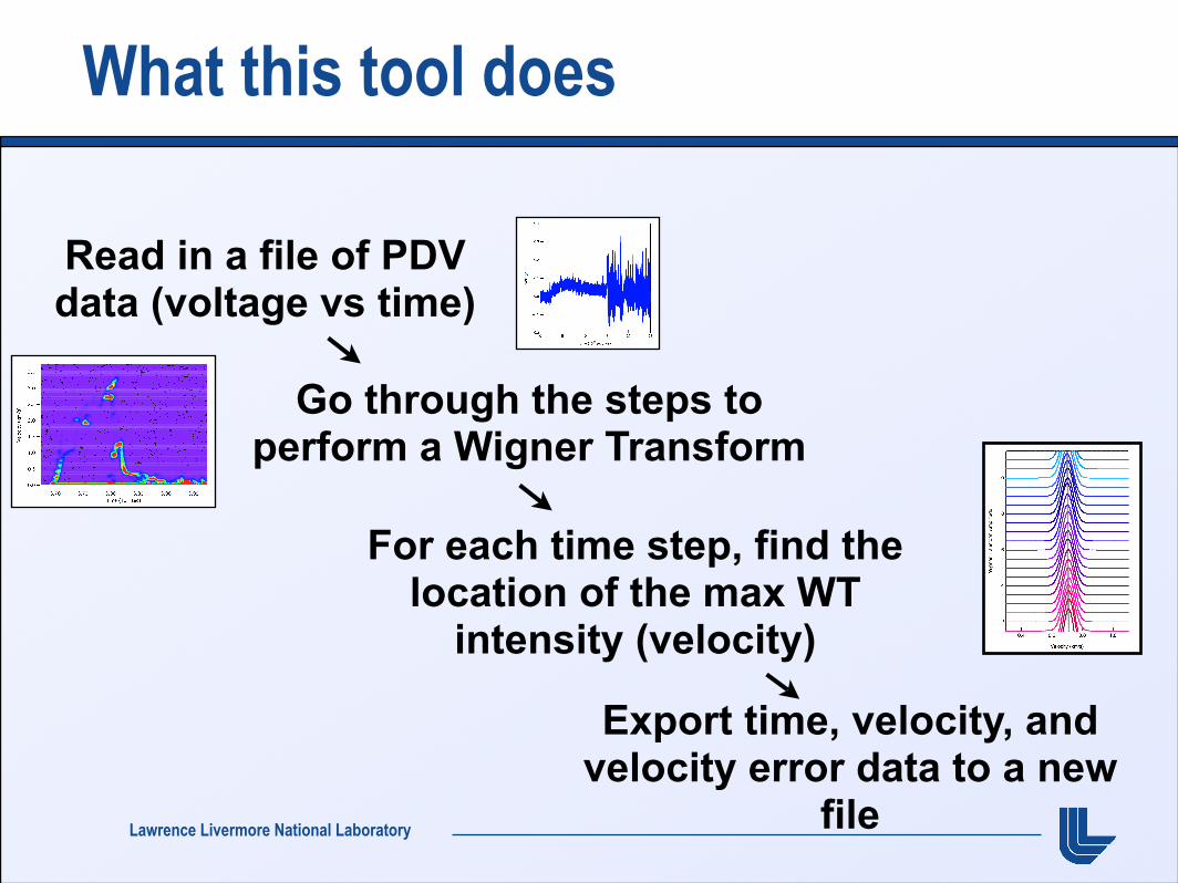
What this tool does

Go through the steps to perform a Wigner Transform

For each time step, find the location of the max WT

intensity (velocity)

Export time, velocity, and velocity error data to a new

file

Read in a file of PDV data (voltage vs time)

Lawrence Livermore National Laboratory

What this tool does

Go through the steps to perform a Wigner Transform

For each time step, find the location of the max WT

intensity (velocity)

Export time, velocity, and velocity error data to a new

file

Read in a file of PDV data (voltage vs time)

Lawrence Livermore National Laboratory

What this tool does

Read in a file of PDV data (voltage vs time)

Go through the steps to perform a Wigner Transform

For each time step, find the location of the max WT

intensity (velocity)

Export time, velocity, and velocity error data to a new

file

Lawrence Livermore National Laboratory

What this tool does

Go through the steps to perform a Wigner Transform

For each time step, find the location of the max WT

intensity (velocity)

Export time, velocity, and velocity error data to a new

file

Read in a file of PDV data (voltage vs time)

Lawrence Livermore National Laboratory

What this tool does

Go through the steps to perform a Wigner Transform

For each time step, find the location of the max WT

intensity (velocity)

Export time, velocity, and velocity error data to a new

file

Read in a file of PDV data (voltage vs time)

Lawrence Livermore National Laboratory

Quick Guide Through the Program

Lawrence Livermore National Laboratory

Load the PDV data and place the cursor at the start

Data from Ted Strand

Lawrence Livermore National Laboratory

Load the PDV data and place the cursor at the start

Data from Ted Strand

Lawrence Livermore National Laboratory

Load the PDV data and place the cursor at the start

Data from Ted Strand

Lawrence Livermore National Laboratory

Click ‘Begin Wigner Transform’ to bring up a zoomed in window

Data from Ted Strand

Lawrence Livermore National Laboratory

Data from Ted Strand

Click ‘Begin Wigner Transform’ to bring up a zoomed in window

Lawrence Livermore National Laboratory

Perform a Wigner transform over this time window

Data from Ted Strand

Lawrence Livermore National Laboratory

Wigner Transform

Graph shows velocity vs time• Red regions show large amplitude• Black regions show low amplitude

−Can be scaled from the left and will be ignored Analyze ROI button creates velocity vs time data

Data from Ralph Hodgin

Lawrence Livermore National Laboratory

Chapter III-9 — Signal Processing

III-298

signal[250,]+=sin(2*pi*x*100/500)WignerTransform /Gaus=100 signalDSPPeriodogram signal // spectrum for comparison

The signal used in this example consists of two “pure” frequencies that have small amount of temporal overlap.

The temporal dependence is clearly seen in the Wigner transform. Note that the horizontal (time) transitions are not sharp. This is mostly due to the application of the minimum uncertainty relation dtdn=1 but it is also due to computational edge effects. By comparison, the spectrum of the signal while clearly showing the presence of two frequencies it pro-vides no indication of the temporal variation of the signal’s frequency content. Further-

-1.5

-1.0

-0.5

0.0

0.5

1.0

1.5

4003002001000s

0.5

0.4

0.3

0.2

0.1

0.0

5004003002001000s

Wigner Transform

Is analogous to creating a musical score• Input sound at a given

frequency vs time• Create an image of

the frequency (velocity) vs time

Chapter III-9 — Signal Processing

III-297

Time Frequency AnalysisWhen you compute the Fourier spectrum of a signal you dispose of all the phase informa-tion contained in the Fourier transform. You can find out which frequencies a signal con-tains but you do not know when these frequencies appear in the signal. For example, consider the signal

.

The spectral representation of f(t) remains essentially unchanged if we interchange the two frequencies f1 and f2. In other words, the Fourier spectrum is not the best analysis tool for signals whose spectra fluctuate in time. One solution to this problem is the so-called “short time Fourier Transform”, in which you can compute the Fourier spectra using a sliding temporal window. By adjusting the width of the window you can determine the time res-olution of the resulting spectra.

Two alternative tools are the Wigner transform and the Continuous Wavelet Transform (CWT).

Wigner TransformThe Wigner transform (also known as the Wigner Distribution Function or WDF) maps a 1D time signal U(t) into a 2D time-frequency representation. Conceptually, the WDF is analogous to a musical score where the time axis is horizontal and the frequencies (notes) are plotted on a vertical axis. The WDF is defined by the equation

Note that the WDF W(t,!) is real (this can be seen from the fact that it is a Fourier transform of an Hermitian quantity). The WDF is also a 2D Fourier transform of the Ambiguity function.

The localized spectrum can be derived from the WDF by integrating it over a finite area dtdn. Using Gaussian weight functions in both t and n, and choosing the minimum uncer-tainty condition dtdn=1, we obtain an estimate for the local spectrum

To illustrate an application of the WignerTransform operation (see page V-700), consider the two-frequency signal:Make/N=500 signalsignal[0,350]=sin(2*pi*x*50/500)

f t( )2"f1t( )sin 0 t t1<#

2"f2t( )sin t1 t t2<#$%&

=

W t !,( ) xU t x 2⁄+( )U' t x 2⁄–( )e i2"x!–d(–

(

)=

W t ! *t;,( ) U t'( ) 2" t t'–*t

----------+ ,- .

2– i2"!t'–( )expexp t'd)

2/

Lawrence Livermore National Laboratory

Wigner Transform

Graph shows velocity vs time• Red regions show large amplitude• Black regions show low amplitude

−Can be scaled from the left and will be ignored Analyze ROI button creates velocity vs time data

Data from Ralph Hodgin

Lawrence Livermore National Laboratory

Data from Ralph Hodgin

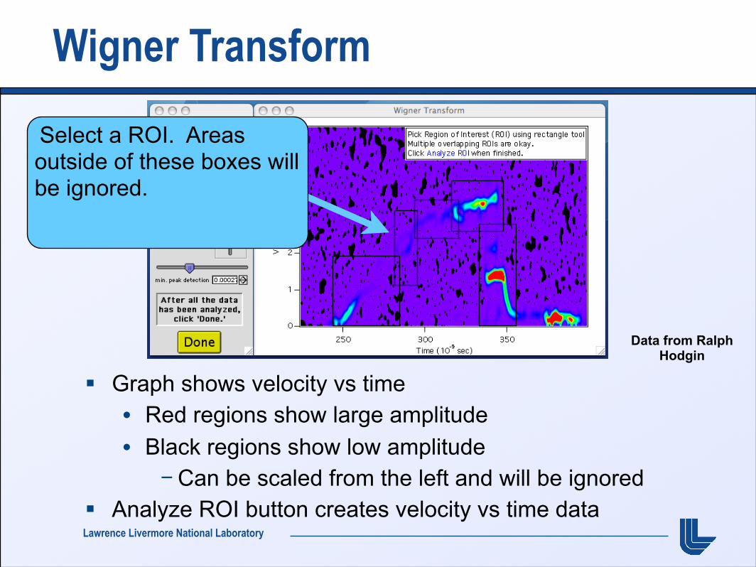
Wigner Transform

Select a ROI. Areas outside of these boxes will be ignored.

Graph shows velocity vs time• Red regions show large amplitude

• Black regions show low amplitude−Can be scaled from the left and will be ignored

Analyze ROI button creates velocity vs time data

Lawrence Livermore National Laboratory

Wigner Transform

Graph shows velocity vs time• Red regions show large amplitude

• Black regions show low amplitude−Can be scaled from the left and will be ignored

Analyze ROI button creates velocity vs time data

Data from Ralph Hodgin

Lawrence Livermore National Laboratory

Graph shows velocity vs time• Red regions show large amplitude

• Black regions show low amplitude−Can be scaled from the left and will be ignored

Analyze ROI button creates velocity vs time data

Data from Ralph Hodgin

Wigner Transform

Lawrence Livermore National Laboratory

Data from Ralph Hodgin

Wigner Transform

Graph shows velocity vs time• Red regions show large amplitude

• Black regions show low amplitude−Can be scaled from the left and will be ignored

Analyze ROI button creates velocity vs time data

Lawrence Livermore National Laboratory

Data from Ralph Hodgin

Wigner Transform

Graph shows velocity vs time• Red regions show large amplitude

• Black regions show low amplitude−Can be scaled from the left and will be ignored

Analyze ROI button creates velocity vs time data

Lawrence Livermore National Laboratory

Velocity vs Time

Each column (time slice) of the Wigner Trans. is analyzed for the maximum intensity• velocity is found by the

location of gaussian peak Final output saves:

• Time

• Velocity

• Velocity Error (Gaussian peak error)

Lawrence Livermore National Laboratory

Perform a Wigner transform over this time window

Data from Ted Strand

Lawrence Livermore National Laboratory

Perform a Wigner transform over this time window

Data from Ted Strand

Lawrence Livermore National Laboratory

Record of Velocity vs Time

Data from Ted Strand

Lawrence Livermore National Laboratory

Go to next section of PDV data and Repeat

Data from Ted Strand

Lawrence Livermore National Laboratory

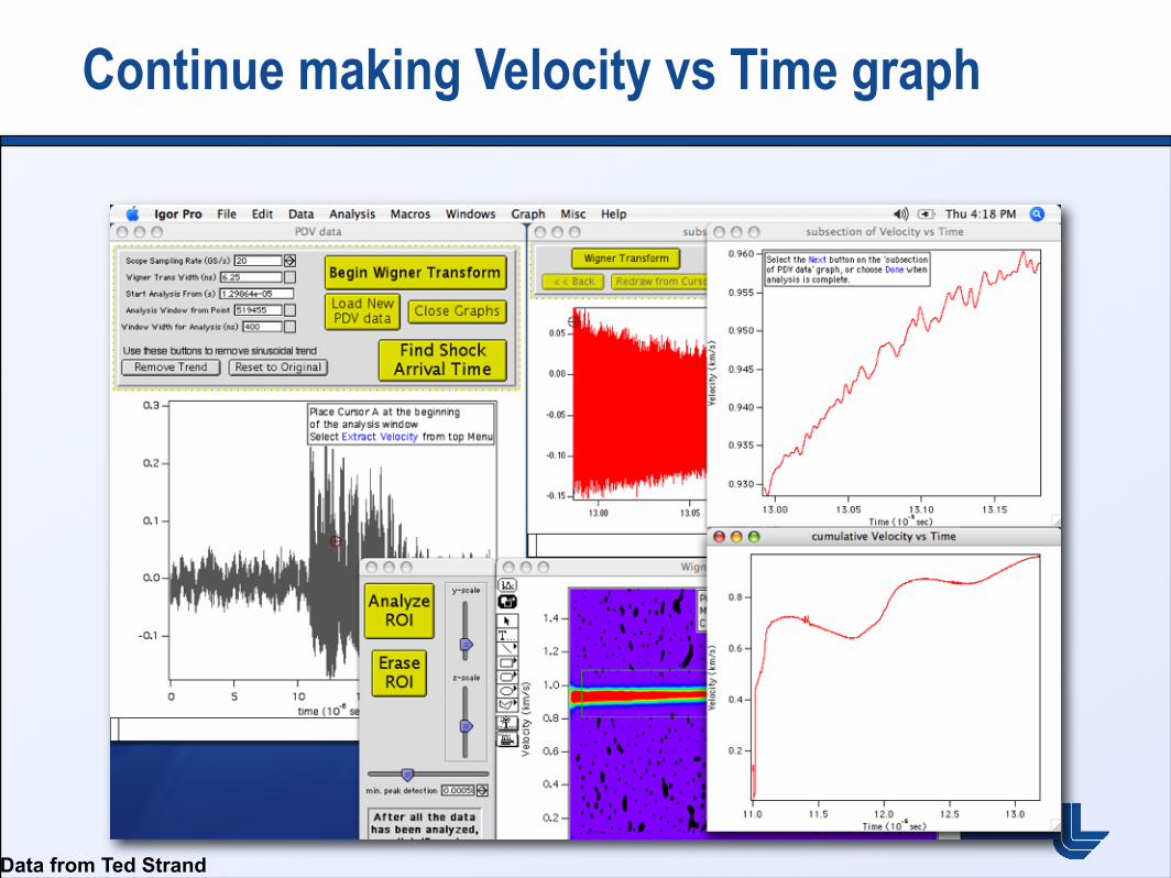
Continue making Velocity vs Time graph

Data from Ted Strand

Lawrence Livermore National Laboratory

Continue making Velocity vs Time graph

Data from Ted Strand

Lawrence Livermore National Laboratory

Continue making Velocity vs Time graph

Data from Ted Strand

Lawrence Livermore National Laboratory

Continue making Velocity vs Time graph

Data from Ted Strand

Lawrence Livermore National Laboratory

Continue making Velocity vs Time graph

Data from Ted Strand

Lawrence Livermore National Laboratory

Continue making Velocity vs Time graph

Data from Ted Strand

Lawrence Livermore National Laboratory

Continue making Velocity vs Time graph

Data from Ted Strand

Lawrence Livermore National Laboratory

Save data to a new file when finished

Data from Ted Strand

Lawrence Livermore National Laboratory

Comparison of Methods

Analyzed via Igor ProAnalyzed via MatLab

26 ns window 6.25 ns window

MatLab reduces data points depending on sampling rate and FFT window size (1:260 in this example)

Lawrence Livermore National Laboratory

Comparison of Methods

“Sliding” FFT, 3.2 ns window, 1.6 ns step size• half-window

overlap Quick - 17 seconds

Pixelated

Data/Analysis by Ralph Hodgin and Chadd May

Lawrence Livermore National Laboratory

Comparison of Methods

“Sliding” FFT, 12.8 ns window, 1.6 ns step size• 1/8-window

overlap 65 seconds to

complete calculation

Pixelated, but much better

Data/Analysis by Ralph Hodgin and Chadd May

Lawrence Livermore National Laboratory

Comparison of Methods

Wigner Transform, 12.8 ns window

5 minutes to complete calculation

Very good resolution

• no loss in data points along time-axis

Lawrence Livermore National Laboratory

Wigner Transform - another great tool for fast time resolved PDV data

Lawrence Livermore National Laboratory

Wigner Transform - another great tool for fast time resolved PDV data

Plasma behind kapton Shock arrival at

front of kapton

Lawrence Livermore National Laboratory

PDV Analysis using Igor Pro

Routine reads in PDV data files• Either Voltage vs time or just Voltage

Goes through sections of the data to perform a Wigner Transform• results in an improved resolution over FFT

Exports a velocity vs time history (csv file)

Can also use to fit a sine wave to the data for determining shock arrival times

Lawrence Livermore National Laboratory

Acknowledgments

Chadd May

Ashok Kumar

Ted Strand

Dave Hare

Ralph Hodgin

Ed Roos

John Weeks (WaveMetrics)

Reed Patterson