Postpr int - DiVA portal695997/FULLTEXT01.pdf · The original publication is available at Tolmachev...

http://www.diva-portal.org

Postprint

This is the accepted version of a chapter published in Human Monoclonal Antibodies: Methods andProtocols.

Citation for the original published chapter :

Tolmachev, V., Orlova, A., Andersson, K. (2014)

Methods for radiolabelling of monoclonal antibodies.

In: Michael Steinitz (ed.), Human Monoclonal Antibodies: Methods and Protocols (pp. 309-330).

Humana Press

Methods in Molecular Biology

http://dx.doi.org/10.1007/978-1-62703-586-6_16

N.B. When citing this work, cite the original published chapter.

Permanent link to this version:http://urn.kb.se/resolve?urn=urn:nbn:se:uu:diva-218570

The original publication is available at www.springerlink.com

Tolmachev V, Orlova A, Andersson K. Methods for radiolabelling of monoclonal antibodies.Methods Mol Biol. 2014;1060:309-30.

http://link.springer.com/protocol/10.1007%2F978-1-62703-586-6_16

Methods for radiolabelling of monoclonal antibodies.

Vladimir Tolmachev1*, Anna Orlova2, Karl Andersson1,3

1Unit of Biomedical Radiation Sciences, Rudbeck Laboratory, Uppsala University, Sweden;

2Preclinical PET Platform, Department of Medicinal Chemistry, Uppsala University, Uppsala,

Sweden;

3 Ridgeview Instruments AB, Uppsala Sweden

* Corresponding author:

Vladimir Tolmachev

Biomedical Radiation Sciences

Rudbeck Laboratory

Uppsala University

S-751 81 Uppsala

Sweden

Phone: +46 18 471 3414

Fax: + 46 18 471 3432

[email protected]

Running head: Radiolabelling of antibodies

Summary

The use of radionuclide labels allow to study the pharmacokinetics of monoclonal antibodies,

to control the specificity of their targeting and to monitor the response to an antibody

treatment with high accuracy. Selection of label depends on the processing of an antibody

after binding to an antigen, and on the character of information to be derived from the study

(distribution of antibody in the extracellular space, target occupancy or determination of sites

of metabolism). This chapter provides protocols for labelling of antibodies with iodine-125

(suitable also for other radioisotopes of iodine) and with indium-111. Since radiolabelling

might damage and reduce the immunoreactive fraction and/or affinity of an antibody, the

methods for assessment of these characteristics of an antibody are provided for control.

Key words: direct radioiodination, indirect radioiodination, CHX-A’’DTPA, indium-111,

iodine-125, immunoreactive fraction, saturation assay, LigandTracer.

1. Introduction

Following fate of antibodies in vivo can provide important information during preclinical

development of antibody- based therapies, during clinical trials and, with the advent of

personalized medicine, in daily clinical practice. The use of radioactive labels for antibodies

facilitates such studies, because it is easy to quantify radioactivity concentration. Moreover,

current imaging techniques, such a single photon emission computed tomography (SPECT)

and positron emission tomography (PET), permit to visualise and quantify distribution of

radioactivity in vivo by non-invasive procedures. Radiolabelled antibodies can be used

during preclinical development for investigation of pharmacokinetics and targeting properties,

dose finding and evaluation of response of treatment, hence speeding-up the process of drug

discovery. The dose finding can be facilitated in clinical trials, reducing the number of

patients treated with suboptimal doses of antibodies. In addition, the radiolabeled antibodies

can be used for selection of patients who have tumours expressing a particular antigen and

may benefit from particular therapy (1).

It has to be taken into account that labelling chemistry can influence cellular retention of

radioactivity. Majority of antibodies are internalized after binding to cell-surface antigens,

either by clathrin-dependent endocytosis or due to the normal turnover of cellular membrane

constituents via non-clathrin-dependent endocytosis (2, 3). After internalization and

translocation into lysosomal compartment, antibodies are proteolytically degraded. In vitro

studies have demonstrated that the fate of a radioactive label after proteolytic degradation

depends on lipophilicity of radiocatabolites (4, 5). Lipophilic radiocatabolites can diffuse

through phospholipide lysosomal and cellular membranes, and leave the malignant cells. Such

fate is typical for vast majority of radiohalogen labels (6). If the radiocatabolites are bulky

hydrophilic (e.g. charged) molecular moiety, they would be retained inside the cells before

excretion by relatively slow externalization. The radiolabels, which are trapped inside the

cells after internalization and degradation of targeting protein, are called “residualizing” or

“trapped”. Radiometals are mainly residualizing labels (7) since their radiocatabolites are

polar and often charged. Accordingly, different labels show different aspects of antibody

distribution in vivo. Radioactivity associated with non-residualizing halogen labels reflects

distribution of an antibody in blood, in extracellular space and bound to membranes of target

cells or to extracellular matrix. Radioactivity associated with residualizing radiometal labels

reflects, along with distribution of antibody outside cells, the amount of antibody, which has

been internalized and degraded inside the tumour cells and by catabolizing organs.

Combination of both residualizing and non-residualizing labels for the same antibody

provides the most complete information concerning its fate in vivo. Resolving gamma-spectra

of radiometal and radiohalogen labels, one can derive such information from a single

biodistribution study, upon co-injection in the same animal of an antibody labelled in two

different ways (8).

One has to be aware that radiolabelling can influence a binding capacity of an antibody. For

example, an oxidative radioiodination of antibodies using Chloramine-T (9) is the most

commonly used method due to its robustness and simplicity. Radioiodide is oxidized in situ

with subsequent attack of nucleophilic side-chains of a protein. A predominant site of

electrophilic iodination at physiological pH is tyrosine (10). It was found (11, 12) that

tyrosine residues are over-represented in complementarity determining regions (CDR) of

antibodies. Iodination of tyrosines in CDR might decrease antigen binding capacity of

antibodies (12). Lysines are presented in CDR to much lesser extent (13), and indirect

halogenation, which is based on coupling of radiolabelled precursor to -amino groups of

lysines, is often safer for proteins. However, over-modification of lysines might be also

unfavourable for binding capacity and biodistribution properties of radiolabelled antibodies.

For this reason, one should take care that a number of pendant group (for radioiodination) or

chelators (for radiometal labelling) should not exceed four-five per a protein molecules. After

labelling of an antibody, the functional properties of antibody binding should be quantified to

verify that adequate binding and acceptable immunoreactive fraction (IRF) is retained. The

minimum level of quality control is to verify that the labelled protein interacts with the

intended target. Since the binding properties of the unlabelled protein may be unknown, the

value produced by the binding assay may serve as a characteristic of the labelled product,

which can be followed over time to prove consistent performance of the labelling protocol.

The saturation assay, which estimates the equilibrium dissociation constant KD is a

representative binding assay that performs well for interactions that reach equilibrium within

one to a few hours. Real-time interaction analysis is a novel and more precise method for

quantifying details of the binding characteristics. It is advantageous for high-affinity

interactions, and requires less work than the manual binding assays, but relies on access to

specialized equipment.

Another aspect of labelling quality is the immunoreactive fraction, i.e. the fraction of the

labelled product, which is capable of binding to the target. The Lindmo assay (14) is the most

commonly used method for assessing immunoreactive fraction.

In this chapter, we provide a description of two methods of radioiodination (a direct

radioiodination using Chloramine-T (Fig.1 A) and indirect radioiodination using N-

succinimidyl 4-thrimethylstannylbenzoate (Fig. 1B)) and labelling with 111In using CHX-A’’-

DTPA (Fig. 1C). The most commonly used method for determination of affinity (saturation

assay) and immunoreactive fraction (Lindmo analysis) of radiolabelled antibodies are also

provided. In addition, a new method for determination of affinity of targeting proteins to

living cells, LigandTracer analysis, is described. Besides an affinity value, this method

provides information concerning association and dissociation kinetics of an antibody

interaction.

[Fig 1 near here]

125I (T1/2 = 60 d) is the most commonly used radionuclide for preclinical studies (in vitro

experiments, biodistribution in small rodents using direct ex vivo measurements, imaging in

mice). This nuclide combines a long half-life with low radiation dose to personnel. The same

protocol may be used for radioiodination using 131I (T1/2 = 8 d) (for e.g. radionuclide therapy,

or for dual-label biodistribution studies), 123I(T1/2 = 13.3 h) (SPECT imaging) and 124I (T1/2 =

4.18 d) (PET imaging). 111In (T1/2 = 2.8 d) is a commercially available radiometal. Its half-live

is compatible with biokinetics of intact IgG. 111In is suitable for in vitro experiments,

biodistribution in small rodents using direct ex vivo measurements, imaging in mice, as well

as for clinical imaging using SPECT/CT.

2. Materials

2.1. Purification of an antibody

1. Milli-Q/ELGA water

2. NAP-5 column (GE Healthcare)

3. Eppendorf tubes (1.7 ml)

4. Antibody solution

5. Automatic pipette 1 ml, pipette tips.

6. Lyophilizing machine (freeze dryer)

2.2. Direct radioiodination of an antibody with 125I using Chloramine-T


2. Electronic balance (0.1 mg)

3. Freeze-dried antibody


5. Eppendorf tubes (1.7 ml)

6. 125I stock solution (GE Healthcare or PerkinElmer)

7. Chloramine-T trihydrate, sodium chloro-(4-methylphenyl)sulfonylazanide (Sigma

or Merck)

8. Sodium metabisulfite, Na2S2O5 (Sigma or Merck)

9. Automatic pipette 5-50 µl, pipette tips.

10. Automatic pipette 1 ml, pipette tips.

11. 0.05M phosphate buffered saline, pH7.4 (PBS)

12. Timer

13. Vortex mixer

14. Dose calibrator set for 125I.

15. Tec-Control Chromatography 150-771 strips (Biodex)

16. 70% acetone/30% water mixture

17. PhosphorImager or TLC scanner (optional).

2.3. Indirect radioiodination of an antibody using N-succinimidyl para-iodobenzoate

N-succinimidyl 4-(trimethylstannyl)benzoate can be synthesized according to method

described by Koziorowski et al (15).


2. 125I stock solution (GE Healthcare or PerkinElmer)

3. Siliconized Eppendorf tubes (1.7 ml)

4. 0.07 M sodium borate, pH 9.3

5. N-succinimidyl 4-(trimethylstannyl)benzoate (ATE)

6. Chloramine-T trihydrate, sodium chloro-(4-methylphenyl)sulfonylazanide

(Sigma or Merck)

7. Sodium metabisulfite, Na2S2O5 (Sigma or Merck)

8. 0.1% aqueous solution of acetic acid

9. 5% acetic acid in methanol


11. Vortex mixer

12. Timer



15. Automatic pipette 1 ml, pipette tips

16. Automatic pipette 2-50 µl, pipette tips

17. Tec-Control Chromatography 150-771 strips (Biodex)

18. 70% acetone/30% water mixture

19. TLC tank

20. Dose calibrator set for 125I.


2.4. Labelling of an antibody with 111In using CHX-A’’DTPA

1. Ion-exchange resin Chelex 100 in sodium form (Sigma)

2. Disposable 0.4 µm filters

3. Disposable syringes

4. Disposable polypropylene 20 ml vials.


6. Siliconized Eppendorf tubes (1.7 ml)

7. 0.07 M sodium borate, pH 9.3, stored over Chelex 100

8. 0.2 M ammonium acetate, pH 5.5, stored over Chelex 100

9. CHX-A’’DTPA, N-[(R)-2-Amino-3-(p-isothiocyanato-phenyl) propyl]-trans-(S,S)-

10. cyclohexane-1,2-diamine-N,N,N’,N”,N”-pentaacetic acid, (Macrocyclics)

11. Vortex mixer

12. Heating block providing 38oC.


14. Automatic pipette 1 ml, pipette tips

15. Automatic pipette 2-50 µl, pipette tips

16. 111In chloride in 0.05 M hydrochloric acid for labelling of antibodies (Covidien)

17. Tec-Control Chromatography 150-771 strips

18. 0.2 M citric acid


2.5. Determination of immumoreactive fraction

1. Cells, adherent or in suspension, 4x107 cells

2. Radiolabelled antibody

3. Non-labelled antibody


5. Polypropylene centrifuge tubes, 15 ml

6. Siliconized Eppendorff tubes

7. Pipette controller (e.g. Pipetboy)

8. Glass or plastic pipettes, 10 ml

9. Set of automatic pipettes 1 µl - 1 ml, pipette tips

10. Cell scraper for adherent cells

11. Vortex mixer

12. Cell counter

13. Centrifuge (at least 5000 g, with timer)

14. Gamma-counter

2.6. Determination of dissociation constant/saturation assay

1. Cells, adherent

2. Radiolabelled antibody

3. Non-labelled antibody


5. Complete cultivation medium for the designated adherent cell line

6. Trypsin-EDTA, 0.25% trypsin, 0.02% EDTA in buffer or other appropriate buffer

for cell detachment

7. Polypropylene centrifuge tubes, 15 ml

8. Disposable cell dishes or 24-well cell plates

9. Siliconized Eppendorf tubes

10. Disposable test tubes

11. Vials for cell counting

12. Pipette controller (e.g. Pipetboy)

13. Disposable plastic pipettes (10 ml)

14. Set of automatic pipettes 1 µl-1 ml, pipette tips

15. Vortex mixer

16. Cell counter

17. Gamma-counter

2.7. LigandTracer

1. Adherent cells, expressing at least 30,000 – 50,000 antigen copies per cell

2. Circular cell dish with 87mm outer bottom diameter (e.g. Nunclon™ cat. No. 150350

or 172958 on www.nuncbrand.com)

3. Cell culture medium, approximately 50 ml

4. Radiolabeled antibody, typically 3-30 µg (depends on the apparent affinity)

5. LigandTracer instrument suitable for the selected radiolabel (125I: LigandTracer Grey,

PET/SPECT radionuclides: LigandTracer Yellow)

3. Methods

3.1. Purification of an antibody

Purification of antibodies is essential for all conjugation labelling techniques. Most

commonly, a conjugation of a chelator or a linker is directed to an amino group of a protein.

Very often, antibody preparations contain free amino acids. The presence of free amino acids

may interfere with amino-directed coupling.

1. Pre-equilibrate the NAP-5 column with Milli-Q water by passing 10 ml of Milli-

Q water through the column.

2. Load 0.5 ml of the antibody solution on the column.

3. Collect and discard first 0.5 ml of eluate.

4. Add 1 ml of Milli-Q water to a column.

5. Collect eluate into an Eppendorf tube.

6. Freeze the eluate at -18 oC for at least 3 hours

7. Freeze-dry the eluate overnight

3.2. Direct radioiodination of an antibody with 125I using Chloramine-T

Important! The work should be performed in a well-ventilated fume-hood. Contamination

control should be performed after labelling.

1. From the freeze-dried antibody, prepare a solution in PBS containing 2 mg/ml.

2. Prepare Eppendorf tubes containing 1-1.5 mg of Chloramine-T and sodium metabisulfite

3. Before starting of labelling, pre-equilibrate a NAP-5 column with PBS, by passing at least

10 ml of the buffer through the column

4. Place 10 µl 125I stock solution into an Eppendorf tube (Note. Up to 20 µl of 125I stock

solution can be used according to this protocol)

5. Add 20 µl antibody solution (40 µg) to the 125I solution.

6. Add 40 µl PBS to the mixture of 125I and the antibody solution.

7. Prepare immediately before labelling a Chloramine-T solution in PBS (1 mg/ml) and

sodium metabisulfite solution (2 mg/ml in PBS)

8. Add 15 µl of Chloramine-T solution in PBS to the mixture of 125I and antibody. Vortex

carefully and incubate the mixture for 60 sec.

9. Add 15 µl sodium metabisulfite solution to the reaction mixture, vortex the mixture

carefully. Calculate the mixture volume, X µl.

10. Load the reaction mixture on the NAP-5 column. Let it pass through the upper filter. Then

add (500-X) µl PBS and let it pass through the upper filter.

11. Collect the eluate as a void volume fraction.

12. Add 1 ml PBS. Collect the eluate a high molecular weight fraction containing the labelled

antibody.

13. Add 1 ml PBS. Collect the eluate a low molecular weight fraction.

14. Cap the column, start with the lower end to reduce the risk of contamination. Measure

activity of empty reaction mixture vial, the high molecular weight fraction, the low

molecular weight fraction and the column to calculate yield according to formula

Yield = [activity of high molecular weight fraction] / [sum of all measured activities]

15. Take 1 µl sample of the high molecular weight fraction and place on Tec-Control

Chromatography 150-771 strip. Elute the strip with the 70% acetone/30% water mixture

16. Evaluate purity of the conjugate. The radiolabelled antibody would stay at the application

point, while free 125I would migrate with the solvent front. This might be done

quantitatively using PhosphorImager or TLC scanner. Alternatively one can cut the Tec-

Control Chromatography 150-771 in the middle. After measurement of background (B),

measure radioactivity of half with the application point (A) and half with the solvent front

(F). Calculate the purity according to formula

P(%) = (A-B)*100/(A+F-2*B)

17. 125I-antibody can typically be stored frozen at -20 oC for a few days

3.3. Indirect radioiodination of an antibody using N-succinimidyl para-iodobenzoate

Important! The work should be performed in a well-ventilated fume-hood. Contamination

control should be performed after labelling.

1. Prepare an Eppendorf tube, containing approx. 1 mg antibody.

2. Prepare Eppendorf tubes containing 1-1.5 mg of Chloramine-T and sodium

metabisulfite.

3. Prepare an Eppendorf tube containing 0.5-1 mg of N-succinimidyl 4-

(trimethylstannyl) benzoate (ATE)

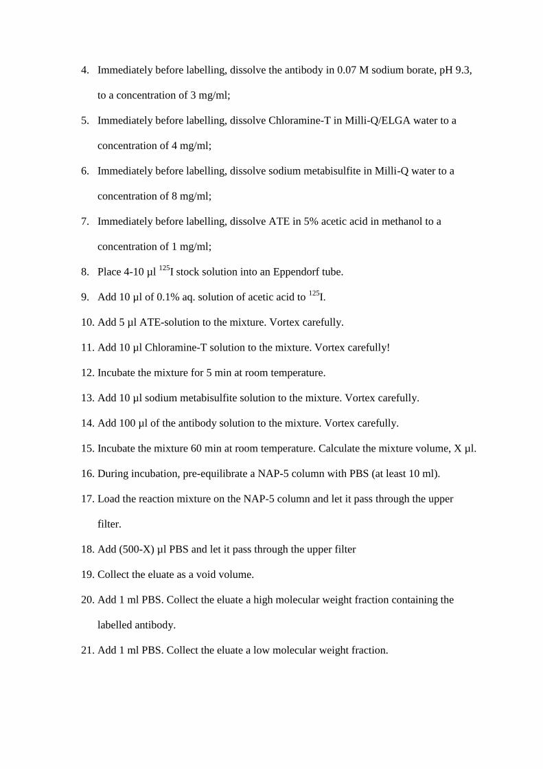
4. Immediately before labelling, dissolve the antibody in 0.07 M sodium borate, pH 9.3,

to a concentration of 3 mg/ml;

5. Immediately before labelling, dissolve Chloramine-T in Milli-Q/ELGA water to a

concentration of 4 mg/ml;

6. Immediately before labelling, dissolve sodium metabisulfite in Milli-Q water to a


7. Immediately before labelling, dissolve ATE in 5% acetic acid in methanol to a


8. Place 4-10 µl 125I stock solution into an Eppendorf tube.

9. Add 10 µl of 0.1% aq. solution of acetic acid to 125I.

10. Add 5 µl ATE-solution to the mixture. Vortex carefully.

11. Add 10 µl Chloramine-T solution to the mixture. Vortex carefully!

12. Incubate the mixture for 5 min at room temperature.

13. Add 10 µl sodium metabisulfite solution to the mixture. Vortex carefully.

14. Add 100 µl of the antibody solution to the mixture. Vortex carefully.

15. Incubate the mixture 60 min at room temperature. Calculate the mixture volume, X µl.

16. During incubation, pre-equilibrate a NAP-5 column with PBS (at least 10 ml).

17. Load the reaction mixture on the NAP-5 column and let it pass through the upper

filter.

18. Add (500-X) µl PBS and let it pass through the upper filter

19. Collect the eluate as a void volume.

20. Add 1 ml PBS. Collect the eluate a high molecular weight fraction containing the

labelled antibody.

21. Add 1 ml PBS. Collect the eluate a low molecular weight fraction.

22. Cap the column, start with the lower end to reduce the risk of contamination. Measure

activity of empty reaction mixture vial, the high molecular weight fraction, the low

molecular weight fraction and the column to calculate yield according to formula

Yield = [activity of high molecular weight fraction] / [sum of all measured activities]

23. Take 1 µl sample of the high molecular weight fraction and place on Tec-Control

Chromatography 150-771 strip. Elute the strip with the 70% acetone/30% water

mixture

24. Evaluate purity of the conjugate using the Tec-Control strips, as it has been described

in 3.2.16. The radiolabeled antibody would stay at the application point, while free 125I

and 125I-iodobenzoic acid would migrate with the solvent front.

3.4. Labelling of antibody with 111In using CHX-A’’DTPA

3.4.1. Preparation of metal-free buffers (see Note 2)

1. Prepare 0.07 M sodium borate, pH 9.3, and 0.2 M ammonium acetate, pH 5.5, using a

high-quality water and p.a. reagents.

2. Add Chelex 100 (10 g per litre of buffer), mix carefully and let stay overnight.

3. Immediately before use, filter the buffer through a 0.4 µm filter into a disposable

polypropylene vial. Use first 5 ml to rinse vials.

3.4.2. Conjugation of CHX-A’’DTPA to an antibody

1. Collect in an Eppendorf tube ~ 1.4 mg freeze-dried antibody. Note the exact weight.

2. Calculate required amount of CHX-A’’DTPA. For a coupling of four chelator per an

antibody molecule, 0.0188 µg CHX-A’’DTPA per 1 µg of antibody is required.

3. Take in an Eppendorf tube 0.7-1.2 mg CHX-A’’DTPA. Note the exact weight.

4. Dissolve CHX-A’’DTPA in 0.07 M sodium borate, pH 9.3, to obtain a final

concentration of 1mg/ml. Use sonication if reagents dissolves slowly.

5. Add a calculated amount of CHX-A’’DTPA in 0.07 M sodium borate, pH 9.3, to the

antibody powder.

6. Add 200 µl of 0.07 M sodium borate, pH 9.3. Vortex the mixture carefully! Calculate

the volume of the solution, X µl.

7. Incubate the reaction mixture for at least 4 h (preferably overnight) at 38 oC.

8. Pre-equilibrate a NAP-5 column with 0.2 M ammonium acetate, pH 5.5, stored over

Chelex 100, by passing at least 10 ml of the buffer through the column.

9. Load the reaction mixture on the column. Let it pass through the upper filter.

10. Add (500-X) µl of 0.2 M ammonium acetate, pH 5.5.

11. Collect and discard the eluate.

12. Add 900 µl of 0.2 M ammonium acetate, pH 5.5, to the column, collect the eluate.

13. You can consider that all your antibody is eluted in 900 µl. Calculate the antibody

concentration.

14. Divide the eluate, containing CHX-A’’DTPA-cetuximab into aliquots containing 100

µg of antibody. The aliquots can be stored frozen at -20 °C.

3.4.3. Labelling of CHX-A’’DTPA cetuximab with 111In

1. Calculate a volume of 111In stock solution required for approx. 10 MBq.

2. Add a required volume of 111In to an aliquot of CHX-A’’DTPA-antibody

conjugate in 0.2 M ammonium acetate, pH 5.5 (100 µg)

3. Vortex the mixture carefully and incubate at room temperature for 1 hour.

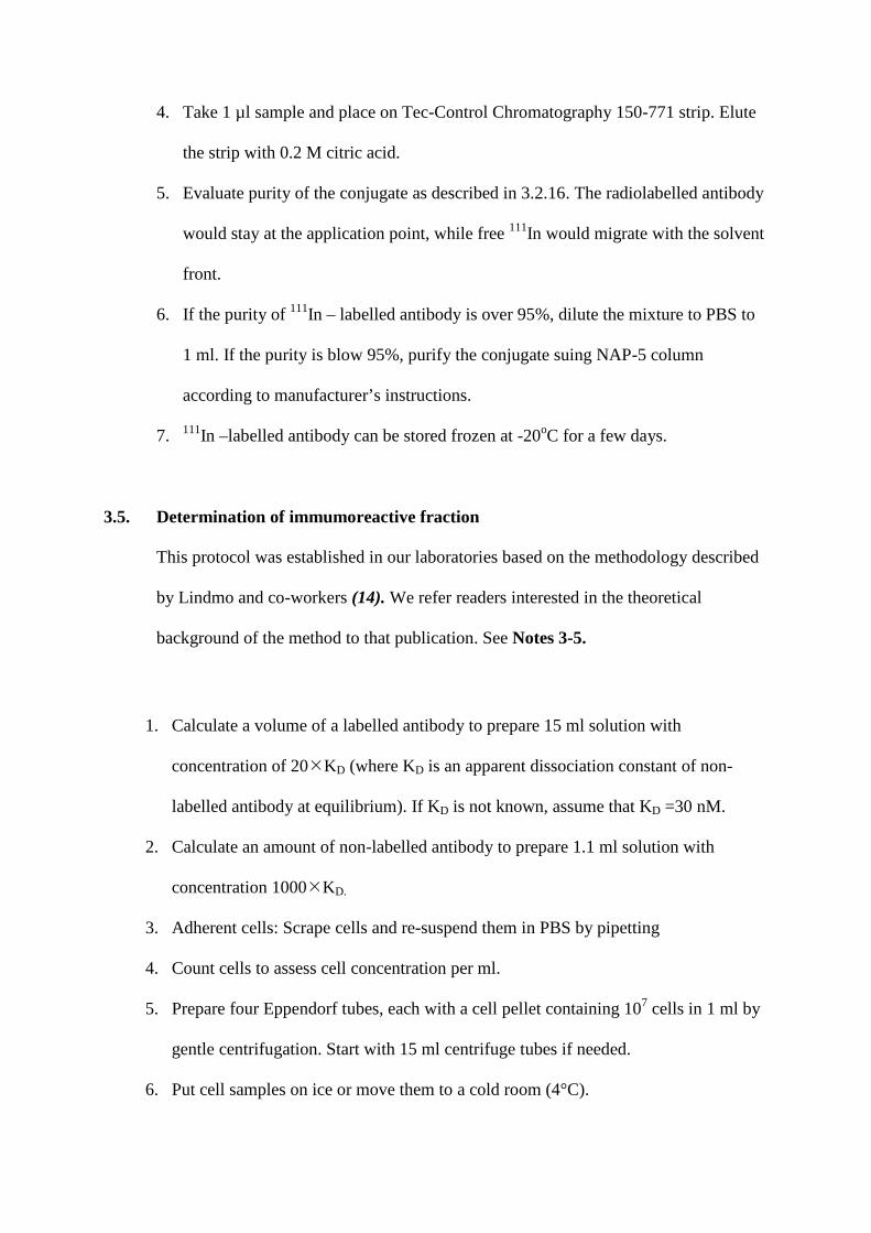
4. Take 1 µl sample and place on Tec-Control Chromatography 150-771 strip. Elute

the strip with 0.2 M citric acid.

5. Evaluate purity of the conjugate as described in 3.2.16. The radiolabelled antibody

would stay at the application point, while free 111In would migrate with the solvent

front.

6. If the purity of 111In – labelled antibody is over 95%, dilute the mixture to PBS to

1 ml. If the purity is blow 95%, purify the conjugate suing NAP-5 column

according to manufacturer’s instructions.

7. 111In –labelled antibody can be stored frozen at -20oC for a few days.

3.5. Determination of immumoreactive fraction

This protocol was established in our laboratories based on the methodology described

by Lindmo and co-workers (14). We refer readers interested in the theoretical

background of the method to that publication. See Notes 3-5.

1. Calculate a volume of a labelled antibody to prepare 15 ml solution with

concentration of 20KD (where KD is an apparent dissociation constant of non-

labelled antibody at equilibrium). If KD is not known, assume that KD =30 nM.

2. Calculate an amount of non-labelled antibody to prepare 1.1 ml solution with

concentration 1000KD.

3. Adherent cells: Scrape cells and re-suspend them in PBS by pipetting

4. Count cells to assess cell concentration per ml.

5. Prepare four Eppendorf tubes, each with a cell pellet containing 107 cells in 1 ml by

gentle centrifugation. Start with 15 ml centrifuge tubes if needed.

6. Put cell samples on ice or move them to a cold room (4°C).

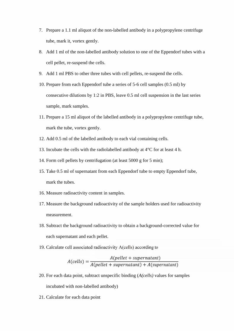
7. Prepare a 1.1 ml aliquot of the non-labelled antibody in a polypropylene centrifuge

tube, mark it, vortex gently.

8. Add 1 ml of the non-labelled antibody solution to one of the Eppendorf tubes with a

cell pellet, re-suspend the cells.

9. Add 1 ml PBS to other three tubes with cell pellets, re-suspend the cells.

10. Prepare from each Eppendorf tube a series of 5-6 cell samples (0.5 ml) by

consecutive dilutions by 1:2 in PBS, leave 0.5 ml cell suspension in the last series

sample, mark samples.

11. Prepare a 15 ml aliquot of the labelled antibody in a polypropylene centrifuge tube,

mark the tube, vortex gently.

12. Add 0.5 ml of the labelled antibody to each vial containing cells.

13. Incubate the cells with the radiolabelled antibody at 4°C for at least 4 h.

14. Form cell pellets by centrifugation (at least 5000 g for 5 min);

15. Take 0.5 ml of supernatant from each Eppendorf tube to empty Eppendorf tube,

mark the tubes.

16. Measure radioactivity content in samples.

17. Measure the background radioactivity of the sample holders used for radioactivity

measurement.

18. Subtract the background radioactivity to obtain a background-corrected value for

each supernatant and each pellet.

19. Calculate cell associated radioactivity A(cells) according to

( ) = ( + )( + ) + ( )20. For each data point, subtract unspecific binding (A(cells) values for samples

incubated with non-labelled antibody)

21. Calculate for each data point

= ( + ) + ( )( )22. Calculate to each data point inverse cell concentration

= lg( )23. Plot a graph of ratio of total added radioactivity to cell bound radioactivity as a

function of inverse cell concentration (ml/cells) and extrapolate the line to

interception with Y axes (X=0) (Figure 2). We recommend using appropriate

program for calculation (e.g. GraphPad Prizm, GraphPad Software Inc).

24. Calculate Immunoreactive fraction as IRF = 100%*1/Y(X=0)

[Fig 2 near here]

3.6. Determination of dissociation constant/saturation assay

1. Prepare a set of four cell culture dishes with adherent antigen-expressing cell

per concentration used, typically 32 – 48 dishes (triplicate plus one cell culture

dish for determination of nonspecific binding by antigen blocking) . Seed cells

in advance, taking in account cells character (doubling time, receptor

expression, time to stable attachment, etc)

2. Calculate the labelled antibody concentrations (8-12 data points) starting from

0.2 KD to 20KD (where KD is an apparent dissociation constant of non-

labelled antibody at equilibrium). If KD value is unknown, we recommend a

concentration range of 200pM-100nM. Remember that actual concentration

added to cell samples will be twice lower! See Notes 6 and 7.

3. Calculate dilution conditions for designed antibody concentrations, typically

1:3 (at least 3 ml solution for every concentration).

4. Calculate the amount of non-labelled protein required to prepare 7 ml solution

with concentration 60KD.

5. Prepare solution of non-labelled antibody in PBS (in a polypropylene

centrifuge tube, 15 ml), mark, vortex gently.

6. Prepare solution of the labelled antibody in PBS (in a polypropylene centrifuge

tube, 15 ml), mark the tube, vortex gently.

7. Prepare a dilution series of labelled antibody solutions according to

calculations using PBS, mark vials, vortex.

8. Wash cells with fresh media.

9. Put culture dishes with cell on ice or move them to cold room (4°C)

10. Add 500 µl of non-labelled antibody solution to one of cell dishes for every

data point, mark. Antigens in this dish will be close to saturated, and the

majority of antibody binding will be unspecific. This dish will be designated as

an unspecific binding control sample.

11. Add 500 µl PBS to all other cell culture dishes.

12. Add 500 µl of the labelled antibody solution with the lowest concentration to

cell culture dishes (triplicate samples plus an unspecific binding control

sample), mark dishes.

13. Take one standard sample (500 µl) to a test tube, mark tube.

14. Repeat these two (12-13) steps for every concentrations

15. Incubate cell samples at 4°C for 4 h

16. After incubation, aspirate the radioactive solution, wash cells with fresh PBS,

detach cells with 0.5 ml trypsin-EDTA solution (or other reagent), add 1 ml

PBS, re-suspend cells, take 0.5 ml for cell counting, collect the rest of cell

suspension to test tubes for measurement, mark test tubes with radioactive

samples.

17. Count cells in all samples.

18. Measure radioactivity in all cell samples and the concentration standards.

19. Measure background radioactivity in the sample holders.

20. Subtract background radioactivity for each sample to obtain background-

corrected values.

21. Calculate the real added radiolabelled antibody concentrations for each data

point assuming that the highest concentration as the most reliable one

(minimum losses due to protein absorption).

22. Calculate measured radioactivity for the highest concentration of added

radiolabelled antibody as counts per minute (CPM) per pmol

23. Calculate bound radioactivity per cell for every sample (e.g. CPM/106 cells)

24. Subtract unspecifically bound radioactivity (radioactivity of the unspecific

binding control sample for this data point) and obtain specifically bound

radioactivity for every data point

25. Calculate specifically bound radioactivity as pmol/106 cells for every sample

26. Plot a graph specifically bound radioactivity per cell (pmol/106 cells) vs.

concentration (pM). Determine Bmax (maximum number of binding sites per

cell) and calculate KD as a concentration of radiolabelled antibody causing

binding equal to Bmax/2 (Figure 3). We recommend using an appropriate

software (e.g. GraphPad Prizm, GraphPad Software Inc). See Notes 8 and 9.

[Fig 3 near here]

3.7. Determination of dissociation constant using LigandTracer.

LigandTracer technology has been described in a series of papers and the technical details of

how to successfully conduct a real-time binding assay on living cells has been discussed

elsewhere (16, 17). Read the instrument instruction booklet prior to starting – standard

operating procedures for maintaining and operating the instrument are clearly described there.

In brief, LigandTracer technology relies on a circular cell dish containing adherent cell in a

limited portions, where the dish is placed on a tilted, slowly rotating support (Figure 4). The

radioactivity detector is placed over the elevated portion of the dish and registers the

additional radioactivity brought under the detector by the cells. Hence, if the radiolabelled

antibody binds to the cells, the detector will register an increased signal when the cells are

below the detector than when the cells are out-of-view. Since the dish rotates continuously,

approximately one data point per minute is collected, making it possible to follow the

progress of the interaction over time.

[Fig 4 near here]

3.7.1. Cell dish preparations

1. Take an 87 mm cell dish and place it tilted on some object (a cell dish lid is usually

fine).

2. Carefully dispense 1-2 ml of cell culture medium containing ~1 million adherent cells

into the lower part.

3. Place in an incubator (still tilted) and let the cells attach firmly. This typically takes 8

hours, but it is strongly dependant on the cell line.

4. When the cells have attached, aspirate the medium, place the dish horizontally, add

~10 ml of cell culture medium, and culture the cells for at least 24 h before using the

dish.

3.7.1. Antibody binding measurement

1. Place the dish in the appropriate LigandTracer device and keep 3 ml of cell culture

medium in the dish. Most LigandTracer assays are conducted at room temperature, but

it is possible to use the device at reduced temperature (+4-8°C) if deemed necessary.

2. Start the device and collect a baseline using the default settings during 3-10 minutes.

3. Stop the device and add a small aliquot of labelled antibody to the dish. Add one µg of

antibody to the three ml liquid already present in the dish, this corresponds to

approximately two nM. Start the device and wait 120-180 minutes.

4. Inspect the shape of the binding curve and compare it to Figure 5.

a. If the first incubation step resulted in a curve approaching equilibrium, stop the

instrument and add two µg antibody to the dish

b. If the first incubation step resulted in a linear curve of increasing signal, stop

the instrument and add nine µg antibody to the dish

c. If no linear or curvilinear signal increase is seen, add nine µg antibody to the

dish

5. Start the device and wait 120-180 minutes.


a. If the first and/or the second incubation step resulted in a curve approaching

equilibrium, stop the instrument and prepare for retention (step 9 below)

b. If the second incubation step resulted in a curve approaching equilibrium, stop

the instrument and prepare for retention (step 9 below)

c. If the first and the second incubation steps resulted in a linear increase of

signal, stop the instrument and add 20 µg antibody to the dish

d. If no linear or curvilinear signal increase is seen, add 20 µg antibody to the

dish

7. Start the device and wait 120-180 minutes.


a. If there is a visible binding signal, prepare for retention (step 9 below)

b. If there is no visible binding signal, stop the measurement and conclude that no

binding can be detected.

9. Retention measurement: Stop the instrument and aspirate the liquid in the cell dish.

Add 3 ml of fresh cell culture medium. It is typically not required to include any wash

steps. Restart the instrument and let it collect data for 3-15 hours.

[Fig 5 near here]

3.7.1. Data analysis

Ocular analysis of the binding trace is often sufficient for a qualitative statement on if the

antibody has the ability to bind the antigen. The most important feature to look for is a

binding signal collected during incubation that approaches equilibrium. (Figure 5 A and B).

Such a curve shape indicates that the antibody binds to a finite number of antigen molecules

on the cells. Exclusively linear uptake curves (Figure 5 C) are inconclusive, but indicate that

either higher concentration (or more time) is needed or that the interaction is unspecific (i.e.

having an infinite or at least very large number of binding sites on the cells). Lack of signal

(Figure 5 D), or square pulses (Figure 5 D), is usually a sign of inability for the antibody to

bind.

The retention measurement which is conducted after replacing the antibody with fresh cell

culture medium reveals how long time the antibody stays in complex with the antigen. Most

antibodies stay bound with their antigen for several hours, resulting in a slowly decreasing

signal (Figure 6 A)

The affinity and the binding kinetics can be resolved through fitting the time-resolved

interaction model to the collected data in specialized software, e.g. TraceDrawer. Such an

analysis can produce precise and accurate estimates on both binding strength (affinity), and

time to equilibrium (binding kinetics), and may even reveal how many parallel processes that

are hidden in one and the same binding trace (Interaction Map). Detailed discussions on

kinetic analysis are beyond the scope of this publication, but plenty of material has been

published elsewhere (18, 19). See Note 10.

[Fig 6 near here]

4. Notes

Note 1. Radionuclides emit ionizing radiation, which is potentially damaging for workers.

During work, the Radiation Safety guidelines set by institutions and the national nuclear

regulatory authorities must be followed strictly and meticulously. Protective equipment,

personal dosimeters and radiation survey monitors are required when handling any radioactive

materials.

Note 2. CHX-A’’DTPA has no particular selectivity for radionuclides and reacts with a broad

range of transitional metals. Metal contaminations may saturate the chelator and prevent

binding of radionuclides. All solution should be prepared using high quality (Milli-Q or

ELGA) water. Buffers should be purified from metal contamination using Chelex 100 resin.

Colourless polypropylene Eppendorf tubes and pipette tips contain usually low level of metal

impurities, and might be used directly. However, care should be taken to prevent them from

dust contamination, as dust might contain metals. For some preparations with very high

specific activity, reaction tubes and pipette tips might additionally treated as described by

Wadas and Anderson (20).

Note 3. Receptor expression on the selected cell line can be a limiting factor in case of low

expression level or high KD value due to receptor depletion. In the sample with highest cell

concentration, antigens have to be in a large excess over antibody.

Note 4. Time to equilibrium in the antibody/antigen interaction can be another limiting factor.

In the case of slow binding kinetics, incubation time should be prolonged.

Note 5. In the case when cell number is not a limiting factor and receptor expression is high,

estimation of Immunoreactive fraction can be done using one data point with cell pellets of 1-

2x107 cells/pellet. In such conditions X0 (21). The Immunoreactive fraction can be

calculated as

= ( + ) ∗ 100%( + ) + ( )Note 6. Radioactivity in solution with the lowest and the highest concentrations added to the

cells have to be measurable using gamma-counter. If radioactivity in solutions for high

concentrations will be too high (causing problems with the dead time of the counter) samples

can be divided in several test tubes. Do not forget to collect pipette tips for radioactivity

measurements.

Note 7. The accuracy of the method depends on accurate estimation of the antibody

concentrations used in the experiment. Take in account that in consecutive dilutions real

protein concentrations can be lower than calculated ones due to absorbance to plastic.

Therefor it is strongly recommended to take a standard sample to every added concentration

and re-calculate the real concentrations based on radioactivity measurements.

Note 8. Internalization of radiolabelled antibodies may influence appreciable the

measurement result leading to overestimation of the bound radioactivity in the case of

residualizing radiometal labels (due to intracellular trapping of internalized antibody) and

underestimation of bound activity in the case of radioiodine labels (due to leakage of

radiocatabolites). For this reason, the assay must be performed at 4oC or on ice, when

internalization is inhibited.

Note 9. Remember that the time to equilibrium depends on concentration, on-rate and off-

rate of the antibody-antigen interaction. In the case of strongly binding antibody (and in

particular low off-rate), time of equilibrium might be equal to several hours or even days. Too

short incubation would cause a serious underestimate of the affinity. For this reason, it is

desirable to evaluate a binding kinetics of an antibody at lowest concentration before

determination of KD and select incubation time when the plateau of uptake is achieved. The

use of LigandTracer is free from this limitation.

Note 10. If the cells detach during the LigandTracer measurement, inaccurate data will be

collected. The detection limit of LigandTracer method depends on the cellular system, but is

typically 30000-50000 receptors per cell.

5. References

1. van Dongen G.A., et al (2007) Immuno-PET: a navigator in monoclonal antibody

development and applications. Oncologist 12, 1379-1389

2. Geissler F., et al (1992) Intracellular catabolism of radiolabeled anti-mu antibodies by

malignant B-cells. Cancer Res 52, 2907-2915

3. Kyriakos R.J., et al (1992) The fate of antibodies bound to the surface of tumor cells in

vitro. Cancer Res 52, 835-842

4. Mattes M.J. et al (1994) Processing of antibody-radioisotope conjugates after binding to

the surface of tumor cells. Cancer 73, 787-793

5. Shih L.B. et al (1994) The processing and fate of antibodies and their radiolabels bound to

the surface of tumor cells in vitro: a comparison of nine radiolabels. J Nucl Med 35, 899-

908

6. Tolmachev V., Orlova A., Lundqvist H.( 2003) Approaches to improve cellular retention

of radiohalogen labels delivered by internalising tumour-targeting proteins and peptides.

Curr Med Chem 10, 2447-2460

7. DeNardo G.L. et al (2004) Radiometals as payloads for radioimmunotherapy for

lymphoma. Clin Lymphoma. 5 Suppl 1:S5-10.

8. Malmberg J. et al (2011) Comparative biodistribution of imaging agents for in vivo

molecular profiling of disseminated prostate cancer in mice bearing prostate cancer

xenografts: focus on 111In- and 125I-labeled anti-HER2 humanized monoclonal

trastuzumab and ABY-025 affibody. Nucl Med Biol 38, 1093-1102

9. Hunter W.M., Greenwood, F.C. (1962) Preparation of iodine-131 labelled human growth

hormones of high specific activity. Nature 194, 495–496

10. Wilbur D.S. (1992) Radiohalogenation of proteins: an overview of radionuclides, labeling

methods, and reagents for conjugate labeling. Bioconjug Chem. 3, 433-470.

11. Olafsen T., et al (1996) Abundant tyrosine residues in the antigen binding site in anti-

osteosarcoma monoclonal antibodies TP-1 and TP-3: Application to radiolabeling. Acta

Oncol. 35, 297-301

12. Nikula T.K., et al (1995) Impact of the high tyrosine fraction in complementarity

determining regions: measured and predicted effects of radioiodination on IgG

immunoreactivity. Mol Immunol. 32, 865-872

13. Olafsen T.,et al (1995) Cloning and sequencing of V genes from anti-osteosarcoma

monoclonal antibodies TP-1 and TP-3: location of lysine residues and implications for

radiolabeling. Nucl Med Biol 22, 765-771

14. Lindmo T., et al. (1984) Determination of the immunoreactive fraction of radiolabeled

monoclonal antibodies by linear extrapolation to binding at infinite antigen excess. J

Immunol Methods. 72, 77–89

15. Koziorowski J., Henssen C., Weinreich R. (1998) A new convenient route to

radioiodinated N-succinimidyl 3- and 4-iodobenzoate, two reagents for iodination of

proteins. Appl Radiat Isot. 49, 955–959

16. Björke H., Andersson K. (2006) Automated, high-resolution cellular retention and uptake

studies in vitro. Appl Radiat Isot. 64, 901-905

17. Björkelund H., et al (2011) Gefitinib induces epidermal growth factor receptor dimers

which alters the interaction characteristics with 125I-EGF. PLoS One 6, e24739

18. Önell A., Andersson K (2005) Kinetic determinations of molecular interactions using

Biacore--minimum data requirements for efficient experimental design. J Mol Recognit.

18, 307-317

19. Björkelund H., Gedda L., Andersson K (2011) Avoiding false negative results in

specificity analysis of protein–protein interactions, J Mol Recognit, 24, 81-89

20. Wadas T.J., Anderson C.J. (2006) Radiolabeling of TETA- and CB-TE2A-conjugated

peptides with copper-64. Nat Protoc. 1, 3062-3068.

21. Wållberg H., et al (2010). Evaluation of the Radiocobalt-Labeled [MMA-DOTA-Cys61]-

ZHER2:2395-Cys Affibody Molecule for Targeting of HER2-Expressing Tumors. Mol

Imaging Biol 12, 54-62.

Figure captions

Figure 1. Labelling of antibodies with 125I by oxidative radioiodination using Chloramine-T(A), indirect radioiodination using N-succinimidyl 4-thrimethylstannylbenzoate (B)-Conjugation of CHX-A’’-DTPA for labelling with 111In (C).

Figure 2. Ratio of total added radioactivity to cell bound radioactivity as a function of inversecell concentration. The immunoreactive fraction was calculated as 1/ Y(X=0)

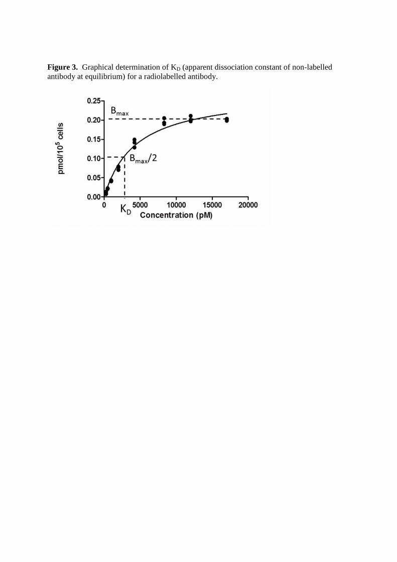
Figure 3. Graphical determination of KD (apparent dissociation constant of non-labelledantibody at equilibrium) for a radiolabelled antibody.

Figure 4. Schematic illustration of LigandTracer technology.

Figure 5. Illustrative examples of two incubation steps of increasing antibody concentrationin a LigandTracer assay. A: Binding curve clearly approaching equilibrium at bothconcentrations is a strong proof for specific interaction. B: First a linear signal increase,followed by the binding curve approaching equilibrium is a strong proof for specificinteraction. C: Linear signal increases at all tested concentrations can have multiple causes,including too low antibody concentration and unspecific interaction, and is henceinconclusive regarding binding properties. D: No or very small signal changes throughout theassay is usually indicative of antibody inability to bind antigens, but may also be due toinsufficient number of cells. E: Square pulse like binding traces is usually indicative ofantibody inability to bind antigens but can have multiple causes, including weak antibodyinteraction.

Figure 6. Antibody trastuzumab (labelled with 125I using the CAT protocol) interacting with HER2expressed on SKOV3 cells, as measured using LigandTracer Grey.

Postpr int - DiVA portal695997/FULLTEXT01.pdf · The original publication is available at Tolmachev...

Documents

Transcript of Postpr int - DiVA portal695997/FULLTEXT01.pdf · The original publication is available at Tolmachev...