Position and Heading Control of an Autonomous Underwater Vehicle using Model Predictive Control

A thesis submitted in fulfilment of the requirements for the degree

of

Master of Technology

in

Electrical Engineering

Specialization

Control & Automation

By

Pankaj Kumar Jha

supervisor

Prof. Bidyadhar Subudhi

Department of Electrical Engineering

National Institute of Technology Rourkela

2011- 2013

i

Department of Electrical Engineering

National Institute of Technology Rourkela

Odisha, India – 769008

CERTIFICATE

This is to certify that the thesis titled “Position and Heading Control of Autonomous

Underwater Vehicle using Model Predictive Control”, submitted to the National Institute

of Technology, Rourkela by Pankaj Kumar Jha, Roll No. 211EE3147 for the award of

Master of Technology in Control & Automation, is a bona fide record of research work

carried out by him under our supervision and guidance.

The candidate has fulfilled all the prescribed requirements.

The Thesis which is based on candidate’s own work, has not submitted elsewhere for a

degree/diploma.

In our opinion, the thesis is of standard required for the award of a Master of Technology

degree in Control & Automation.

To the best of our knowledge, he bears a good moral character and decent behaviour.

Place : Rourkela Prof. Bidyadhar Subudhi Date :

ii

Acknowledgements

There are many people whose help and timely suggestions have helped

throughout this project and are highly appreciable for completion of this project.

First, I would like to thank my thesis supervisor Prof. Bidyadhar Subudhi for his

support and constant encouragements, valuable discussions without which my

work may not be in present form. The discussion held with the friends and

research scholars of control and robotics lab is worth to mention especially with

Khushal Chaudhari and Ankush Kumar. I am thank full to Professor A. K.

Panda, Sandip Ghosh, S. Maity, Subhojit Ghosh and S. Samanta of the

Electrical Engineering department for their course work and constant

encouragement which helped me in completing my thesis work. Thanks to those

who are also the part of this project whose names could have not been

mentioned here. I highly acknowledge the financial support made by Ministry

of Human Resource and Development so as to meet the expenses for study.

Lastly, I mention my indebtedness to my Father and mother for their love and

affection and their constant support which made me believe in me.

Pankaj Kumar Jha

iii

ABSTRACT

Autonomous Underwater Vehicle (AUV) is currently being used for scientific research, commercial and military underwater applications. AUV requires autonomous guidance and control systems to perform underwater applications. This Thesis is concerned with position and heading control of AUV using Model Predictive Control.

Position control is a typical motion control problem, which is concerned with the design of control laws that force a vehicle to reach and maintain a fixed position. The position control of body fixed x-axis to a fixed point using MPC toolbox of MATLAB is done here. System is modelled Using INFANTE AUV hydrodynamic parameters. There is physical limitation on thruster value. Heading control is concerned with the design of control laws that force a vehicle to reach and maintain a fixed direction. There are physical limitations on control input (Rudder deflection) in heading control also a high yaw rate can produce sway and roll motion, which makes it necessary to put constraint on yaw rate. The MPC have a clear advantage in case of control and input constraints. To avoid constraint violation and feasibility issues of MPC for AUV heading control Disturbance Compensating (DC) MPC scheme is used. The DC-MPC scheme is used for ship motion control and gave better results so we are using the proposed scheme to AUV heading control.

A 2 DOF AUV model is taken with yaw rate and rudder deflection constraints. Line of sight (LOS) guidance scheme is utilised to generate the reference heading, which is to be followed. Two types of disturbances are taken constant and sinusoidal. Then simulation has been done for standard MPC, M-MPC and DC-MPC. A (DC) MPC algorithm is used to satisfy the state constraints in presence of disturbance to get a better performance.

Standard MPC gives good result without disturbance. But in case of disturbance yaw constraint is violated. At many time steps the standard MPC has no solution for given yaw rate constraint at those time steps the constraints have been removed. The M-MPC satisfies the constraints. The DC-MPC gives better result in comparison to standard MPC and Modified MPC. The steady state oscillations are less in DC-MPC as compared to M-MPC for sinusoidal disturbances.

The minimization of extra cost function in DC-MPC makes the result better than M-MPC. By solving the extra cost function we try to make response close to that of without disturbance. The only added complexity in DC-MPC is ni-dimensional optimization problem. Which is very less compared to Np*ni, complexity of M-MPC. Where ni is the dimension of control input and Np is value of prediction horizon. The feasibility of DC-MPC scheme largely depends on the magnitude of disturbance. If disturbance is too large then this scheme is not feasible.

iv

CONTENTS CERTIFICATE ii

ACKNOWLEDGMENT iii

ABSTRACT iv

CONTENTS v

LIST OF TABLES vi

LIST OF FIGURES vii

ACRONYMS vii

CHAPTER 1: Introduction

1.1 AUV structure 1

1.2 Literature review on MPC 4

1.3 Thesis objective 5

1.4 Organization of thesis 5

CHAPTER 2: Position Control of an AUV

2.1 Introduction 6

2.2 Problem statement 6

2.3 AUV kinematics and dynamics 6

2.4 Chapter summary 7

CHAPTER 3: Design of Model Predictive Control for an AUV

3.1 MPC control design 8

3.2 Result and Discussions 9

3.3 Chapter summary 12

CHAPTER 4: Heading control of an AUV

4.1 Introduction 13

4.2 Problem statement 13

4.3 System modelling 15

4.4 Chapter Summary 17

v

CHAPTER 5: Design of Model Predictive Control for an AUV

5.1 Design of Standard MPC 18

5.2 Design of Modified MPC 19

5.3 Design of Disturbance compensated MPC 20

5.4 Result and Discussions 22

5.5 Chapter summary 28

CHAPTER 6: Conclusion and Suggestions for future work 29

REFERENCES 30

LIST OF TABLES

Table 2.3.1: Hydrodynamic coefficient of INFANTE AUV. 7

Table 3.2.1: MPC controller parameters. 9

Table 3.2.2: MPC controller parameters. 11

Table 4.3.1: Different Hydrodynamic coefficient of INFANTE MARIUS AUV 16

Table 4.3.2: Hydrodynamic coefficients for the INFANTE MARIUS AUV 16

Table 5.4.1: Difference between M-MPC and DC-MPC with Sinusoidal disturbance. 28

LIST OF FIGURES

Figure 1.1.1: Expanded view of AUV. 1

Figure 1.1.2: AUV coordinate system 2

Figure 2.1.1: Position control block diagram 6

Figure 3.1.1: Model Predictive Control 9

Figure 3.2.1: Position in x direction vs. time 10

Figure 3.2.2: Thrust force vs. time 10

Figure 3.2.3: Position in x direction vs. time 11

Figure 3.2.4: Thrust force (control input) vs. time 11

Figure 4.2.1: Block diagram of heading control 13

vi

Figure 4.2.1: Heading and Rudder angle with Earth Co-ordinates. 14

Figure 4.2.2: AUV-target engagement geometry 15

Figure 5.4.1: Yaw rate (rad/sec) vs. Time (sec) for standard MPC 23

Figure 5.4.2: Heading angle (deg) vs. Time (sec) for standard MPC 23

Figure 5.4.3: Rudder angle (deg) vs. Time (sec) for standard MPC 24

Figure 5.4.4: Yaw rate vs. Time for M-MPC with constant disturbance 24

Figure 5.4.5: Heading angle vs. Time for M-MPC with constant disturbance 24

Figure 5.4.6: Rudder angle vs. Time for M-MPC with constant disturbance 25

Figure 5.4.7: Yaw rate vs. Time for M-MPC with sinusoidal disturbance 25

Figure 5.4.8: Heading angle vs. Time for M-MPC with sinusoidal disturbance 25

Figure 5.4.9: Rudder angle vs. Time for M-MPC with sinusoidal disturbance 26

Figure 5.4.10: Yaw rate vs. Time for DC-MPC with constant disturbance 26

Figure 5.4.11: Heading angle vs. Time for DC-MPC with constant disturbance 26

Figure 5.4.12: Rudder angle vs. Time for DC-MPC with constant disturbance 27

Figure 5.4.13: Yaw rate vs. Time for DC-MPC with sinusoidal disturbance 27

Figure 5.4.14: Heading angle vs. Time for DC-MPC with sinusoidal disturbance 27

Figure 5.4.15: Rudder angle vs. Time for DC-MPC with sinusoidal disturbance 28

ACRONYMS

AUV Autonomous Underwater Vehicles

MPC Model Predictive Control

DC Disturbance Compensation

DOF Degree of Freedom

M-MPC Modified-MPC

GYRO Gyroscope

GPS Global Positioning System

LOS Line of Sight

vii

CHAPTER 1

INTRODUCTION 1.1 AUV STRUCTURE At Applied Physics Laboratory University of Washington in 1957 by Stan Murphy, Bob Francois and later by, Terry Ewart first AUV was developed. The "Special Purpose Underwater Research Vehicle (SPURV)", was used to detect waves created by submarine, to study diffusion and acoustic transmission. Other early AUVs were designed and developed at the Massachusetts Institute of Technology in the 1970s.

An Autonomous Underwater Vehicle is an undersea system which has its own power and controlled by an onboard computer while doing a pre-defined task [1] AUVs contains closely packed devices, it is self-contained i.e. complete and independent unit in itself, low-drag profile crafts powered mostly by a single underwater DC power thruster. The vehicle consist on-board computers for decision making, power source and vehicle payloads for automatic navigation, control and guidance. They can be equipped with state-of-the-art scientific sensors to measure oceanic properties, or specialized biological and chemical pay-loads to detect marine life [2]. As common in most developments today, AUVs have been operated in a semi-autonomous mode under human supervision; they can be tracked, monitored, or even halted during a mission so as to change the mission plan.

Main components of AUV

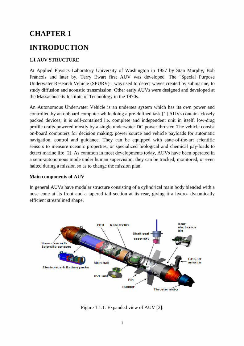
In general AUVs have modular structure consisting of a cylindrical main body blended with a nose cone at its front and a tapered tail section at its rear, giving it a hydro- dynamically efficient streamlined shape.

Figure 1.1.1: Expanded view of AUV [2].

1

Pressure Hull provides the majority of the buoyancy for the vehicle and space for components such as batteries and control electronics. Tail cone is like a torpedo tail, and is designed to reduce the drag caused by the pressure drop at the end of the vehicle body. Nose section consists of scientific sensors like forward look sonar which helps in navigation. Main section encompasses of electronic circuitry, batteries, Rate GYRO. Rate GYRO is used to measure the yaw of the vehicle, main CPU, and Doppler Velocity Log (DVL) sensor that allows the vehicle to know the approximate distance it travelled in three orthogonal axes. Fins help in swimming. Rudder is the vertical and movable control, which is hinged to the fin and mainly controls the yawing movement of the vehicle. Thruster motor provides the necessary thrust to move in forward direction GPS antenna used to locate the exact position of AUV.

Factors Affecting an Underwater Vehicle Motion

Buoyancy is the ability of an object to float depends on whether or not the magnitude of the weight of the body, W, is greater than the buoyant force B. Hydrodynamic Damping Main forces acting in the opposite direction to the motion of the body mainly due to drag and lifting forces. Stability if centres of mass, CM, and buoyancy, CB are not aligned vertically with each other in either the longitudinal or lateral directions, then instability will exist due to the creation of a nonzero moment. Environmental Forces can affect the motion and stability of a vehicle.

AUV Coordinate System

Analogous to flying vehicles, an underwater vehicle has 6DOF. three spatial coordinates x, y and z ; and three attitude defining Euler angles, roll(phi) , pitch(theta) , and yaw(psi) .

Figure 1.1.2: AUV coordinate system [15].

2

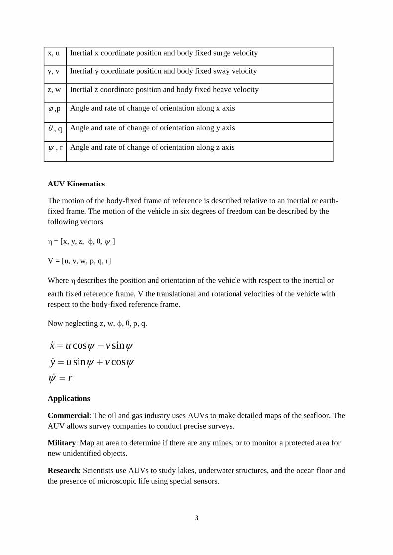
x, u Inertial x coordinate position and body fixed surge velocity

y, v Inertial y coordinate position and body fixed sway velocity

z, w Inertial z coordinate position and body fixed heave velocity

ϕ ,p Angle and rate of change of orientation along x axis

θ , q Angle and rate of change of orientation along y axis

ψ , r Angle and rate of change of orientation along z axis

AUV Kinematics

The motion of the body-fixed frame of reference is described relative to an inertial or earth-fixed frame. The motion of the vehicle in six degrees of freedom can be described by the following vectors

h = [x, y, z, f, q, ψ ]

V = [u, v, w, p, q, r]

Where h describes the position and orientation of the vehicle with respect to the inertial or

earth fixed reference frame, V the translational and rotational velocities of the vehicle with respect to the body-fixed reference frame.

Now neglecting z, w, f, q, p, q.

cos sinsin cos

x u vy u v

r

ψ ψψ ψ

ψ

= −= +=

Applications

Commercial: The oil and gas industry uses AUVs to make detailed maps of the seafloor. The AUV allows survey companies to conduct precise surveys.

Military: Map an area to determine if there are any mines, or to monitor a protected area for new unidentified objects.

Research: Scientists use AUVs to study lakes, underwater structures, and the ocean floor and the presence of microscopic life using special sensors.

3

1.2 LITERATURE REVIEW ON MODEL PREDICTIVE CONTROL

Typical nonlinear control methodologies do not take input and output constraints explicitly into account in the design process, the constraint enforcement is often achieved through numerical simulations and trial-and-error tuning of the controller parameters. Few other control methodologies, such as the Model Predictive Control (MPC) [7] have a clear advantage in addressing input and state constraints explicitly. MPC refers to a class of algorithms which compute a sequence of manipulated variable adjustments to optimize the future behaviour of a plant.

MPC was first given by Richalet, Rault, Testud and Papon (1976) for process control, several proposals for MPC had already been made, by Lee and Markus, and, even earlier a proposal, by Propoi (1963), of a form of MPC for linear systems using linear programming with hard constraints on control was given. MPC proposed in Richalet et al. (1976, 1978), employs a finite horizon pulse response (linear) model, on a quadratic cost function, and input and output constraints. Least square estimation was used.

As in dynamic matrix control (DMC; Cutler & Ramaker, 1980; Prett & Gillette, 1980), which uses a step response model but similar in other aspects the treatment of control and output constraints is ad hoc. This limitation was overcome in the second-generation program, quadratic dynamic matrix control (QDMC; GarcmHa & Morshedi, 1986) where quadratic programming is used to solve exactly the constrained open-loop optimal control problem when the system is linear, the cost quadratic, and the control and state constraints are defined by linear inequalities. QDMC also allows, if needed, temporary violation of some output constraints.

MPC technology from the past to the future has been reviewed by Morari and Lee (1999) while Carlos et al., (1989) gave comparison between both theoretical and practical aspects of MPC.

In [10], rudder saturation in the MPC controller for tracking control of marine surface vessels is considered, and in [11], the roll reduction for the heading control problem using an MPC approach is achieved. However, no state constraints, such as yaw rate and roll angle, are explicitly considered in [11]. The path following with input (rudder) and state (roll) constraints is achieved via MPC in [8].

MPC is a control technique, which includes optimization within feedback to deal with systems subject to constraints on inputs and states [7], [8]. Using an explicit model, and the current measured or estimated state as the initial state to predict the future response of a plant, MPC determines the control action by solving a finite-horizon open-loop optimal control problem online at each sampling interval. Furthermore, it can be applied to multi-variable systems, MPC can handle under-actuated or over-actuated problem easily by combining all the objectives into a single objective function. One of the primary reasons for the success of MPC in industrial applications is its capability in enforcing various types of constraints on the

4

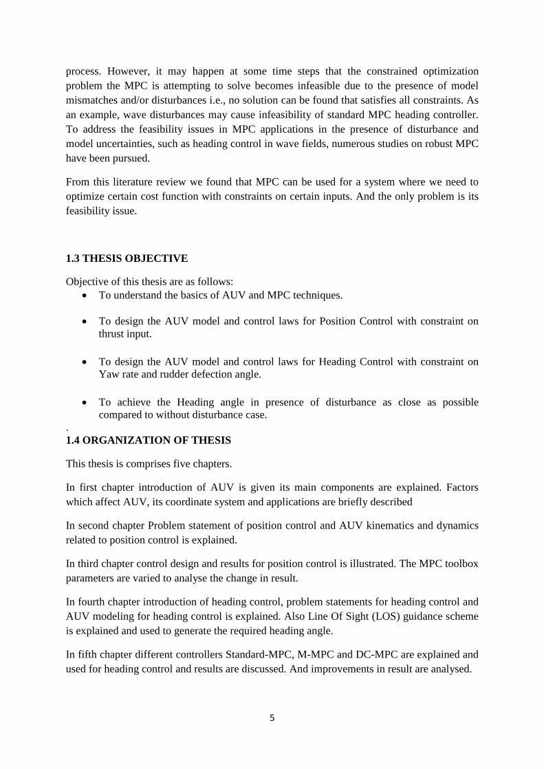
process. However, it may happen at some time steps that the constrained optimization problem the MPC is attempting to solve becomes infeasible due to the presence of model mismatches and/or disturbances i.e., no solution can be found that satisfies all constraints. As an example, wave disturbances may cause infeasibility of standard MPC heading controller. To address the feasibility issues in MPC applications in the presence of disturbance and model uncertainties, such as heading control in wave fields, numerous studies on robust MPC have been pursued.

From this literature review we found that MPC can be used for a system where we need to optimize certain cost function with constraints on certain inputs. And the only problem is its feasibility issue.

1.3 THESIS OBJECTIVE

Objective of this thesis are as follows: • To understand the basics of AUV and MPC techniques.

• To design the AUV model and control laws for Position Control with constraint on

thrust input.

• To design the AUV model and control laws for Heading Control with constraint on Yaw rate and rudder defection angle.

• To achieve the Heading angle in presence of disturbance as close as possible compared to without disturbance case.

. 1.4 ORGANIZATION OF THESIS

This thesis is comprises five chapters.

In first chapter introduction of AUV is given its main components are explained. Factors which affect AUV, its coordinate system and applications are briefly described

In second chapter Problem statement of position control and AUV kinematics and dynamics related to position control is explained.

In third chapter control design and results for position control is illustrated. The MPC toolbox parameters are varied to analyse the change in result.

In fourth chapter introduction of heading control, problem statements for heading control and AUV modeling for heading control is explained. Also Line Of Sight (LOS) guidance scheme is explained and used to generate the required heading angle.

In fifth chapter different controllers Standard-MPC, M-MPC and DC-MPC are explained and used for heading control and results are discussed. And improvements in result are analysed.

5

CHAPTER 2

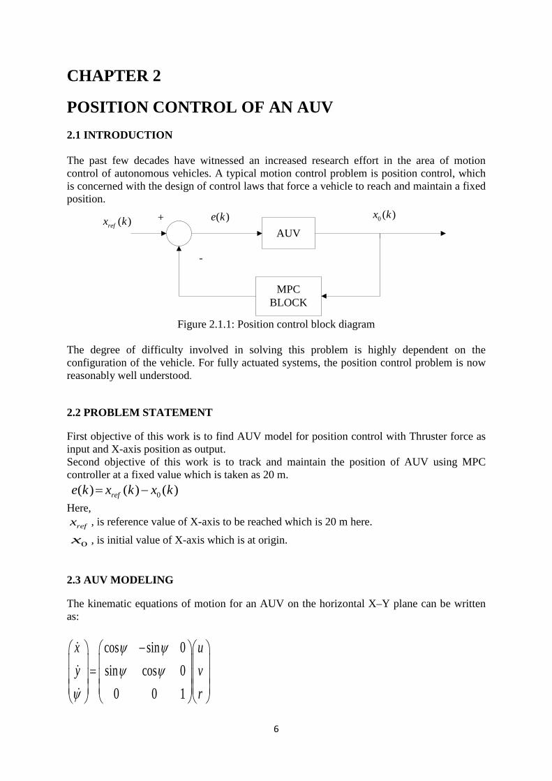
POSITION CONTROL OF AN AUV 2.1 INTRODUCTION The past few decades have witnessed an increased research effort in the area of motion control of autonomous vehicles. A typical motion control problem is position control, which is concerned with the design of control laws that force a vehicle to reach and maintain a fixed position.

AUV

MPC BLOCK

( )refx k 0 ( )x k( )e k+

-

Figure 2.1.1: Position control block diagram

The degree of difficulty involved in solving this problem is highly dependent on the configuration of the vehicle. For fully actuated systems, the position control problem is now reasonably well understood.

2.2 PROBLEM STATEMENT

First objective of this work is to find AUV model for position control with Thruster force as input and X-axis position as output. Second objective of this work is to track and maintain the position of AUV using MPC controller at a fixed value which is taken as 20 m. 0( ) ( ) ( )refe k x k x k= −

Here, refx , is reference value of X-axis to be reached which is 20 m here.

0x , is initial value of X-axis which is at origin.

2.3 AUV MODELING

The kinematic equations of motion for an AUV on the horizontal X–Y plane can be written as:

cos sin 0sin cos 0

0 0 1

x uy v

r

ψ ψψ ψ

ψ

− =

6

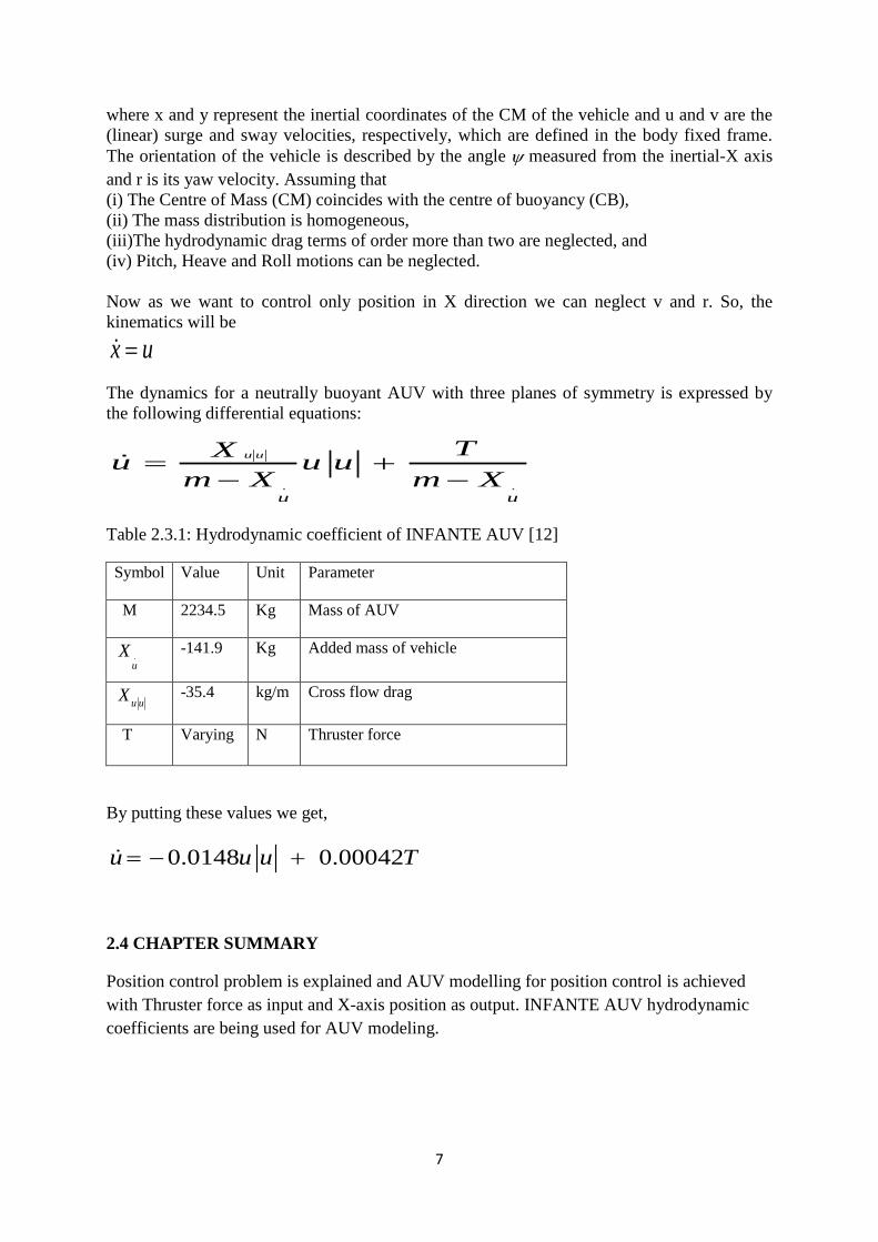
where x and y represent the inertial coordinates of the CM of the vehicle and u and v are the (linear) surge and sway velocities, respectively, which are defined in the body fixed frame. The orientation of the vehicle is described by the angle ψ measured from the inertial-X axis and r is its yaw velocity. Assuming that (i) The Centre of Mass (CM) coincides with the centre of buoyancy (CB), (ii) The mass distribution is homogeneous, (iii)The hydrodynamic drag terms of order more than two are neglected, and (iv) Pitch, Heave and Roll motions can be neglected. Now as we want to control only position in X direction we can neglect v and r. So, the kinematics will be

x u=

The dynamics for a neutrally buoyant AUV with three planes of symmetry is expressed by the following differential equations:

. .

u u

u u

TXu u um X m X

= +− −

Table 2.3.1: Hydrodynamic coefficient of INFANTE AUV [12]

Symbol Value Unit Parameter

M 2234.5 Kg Mass of AUV

.u

X -141.9 Kg Added mass of vehicle

u uX -35.4 kg/m Cross flow drag

T Varying N Thruster force

By putting these values we get,

0.0148 0.00042u u u T= − +

2.4 CHAPTER SUMMARY

Position control problem is explained and AUV modelling for position control is achieved with Thruster force as input and X-axis position as output. INFANTE AUV hydrodynamic coefficients are being used for AUV modeling.

7

CHAPTER 3

DESIGN OF MODEL PREDICTIVE CONTROL FOR AN AUV

3.1 MPC CONTROL DESIGN

MPC is introduced to the process industry in the late 1970s. The cost function calculates the desired control signal by using a model of the plant to predict future plant outputs. Typically, the criterion is the difference between the predicted process output and the desired reference trajectory. A simple objective function is:

1

1 0ˆ ˆ( ) ( )

CP HHT T

ref refj i

J x x Q x x T R T−

= == − − + ∆ ∆∑ ∑

With the constraint on Thrust input given as follows:

20T ≤

Where, x is the predicted process output or AUV position, refx is the reference position, and

H p is the Prediction horizon. This criterion is chosen so that controller output sequence T

0ver the prediction horizon is obtained by minimisation of J with respect to T∆ . As a result the future tracking error is minimised. If there are no model mismatches i.e. the model is identical to the process and there are no disturbances and no constraints, the process will track the reference trajectory exactly on the sampling instants. MPC algorithm consists following steps:

i) It uses an explicit model to predict the process output along a future time horizon

called Prediction Horizon. ii) It then calculate a control sequence along a future time horizon (Control Horizon), to

optimise a performance index. iii) A receding horizon strategy is used so that at each instant the horizon is moved

towards the future, in which first control signal of the sequence calculated at each step is used.

8

Optimiser AUV

Model

CostFunction Constraints

T(k-d)Set

point

( )refx k i+

ˆ( )x k i+

( )e k i+

( )x k

MODEL PREDICTIVE CONTROLLER

Figure 3.1.1: Model Predictive Control

3.2 RESULT AND DISCUSSIONS

In simulation MPC toolbox is used to control the x position at a fixed value 20 m. A subsystem is designed for AUV dynamics. The output of subsystem is x(k) which is given to the MPC block as input variable and the output variable of MPC is thrust which is control input. The thrust value is constraint between -20 N to 20 N. First model is linearized to a two integrator model by MPC toolbox which is having two states 1x and 2x .The state equation is given as:

[ ].

1 11.

22

0 0 0.0004201 0

xxu

xx

= +

The output equation is given as:

[ ] 1

2

0 1x

yx

=

Operating points = 0

Then results are taken by varying control interval.

Table 3.2.1: MPC controller parameters

Control interval (sec) 1 Prediction horizon 10 Control horizon 2 Estimator gain 0.5 Input Weight 0.1 Output Weight 1

9

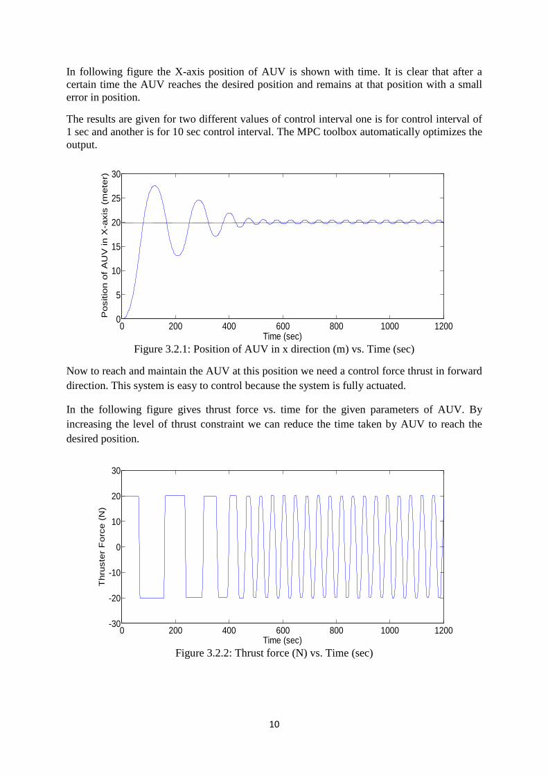
In following figure the X-axis position of AUV is shown with time. It is clear that after a certain time the AUV reaches the desired position and remains at that position with a small error in position.

The results are given for two different values of control interval one is for control interval of 1 sec and another is for 10 sec control interval. The MPC toolbox automatically optimizes the output.

Figure 3.2.1: Position of AUV in x direction (m) vs. Time (sec)

Now to reach and maintain the AUV at this position we need a control force thrust in forward direction. This system is easy to control because the system is fully actuated.

In the following figure gives thrust force vs. time for the given parameters of AUV. By increasing the level of thrust constraint we can reduce the time taken by AUV to reach the desired position.

Figure 3.2.2: Thrust force (N) vs. Time (sec)

0 200 400 600 800 1000 12000

5

10

15

20

25

30

Time (sec)

Pos

ition

of

AU

V in

X-a

xis

(met

er)

0 200 400 600 800 1000 1200-30

-20

-10

0

10

20

30

Time (sec)

Thr

uste

r F

orce

(N

)

10

Now we increase the Control interval for MPC toolbox to 10 sec then the variation is analysed for same reference and constraints for AUV Position control.

Table 3.2.2: MPC controller parameters

Control interval (sec) 10 Prediction horizon 10 Control horizon 2 Estimator gain 0.5 Input Weight 0.1 Output Weight 1

Figure 3.2.3: Position of AUV in X direction (m) vs. Time (sec)

Figure 3.2.4: Thruster force (N) vs. Time (sec)

Result clearly shows that by increasing the control interval the AVU reaches the desired position faster and the steady state oscillation also removed from position vs. time curve. Also the variation in Thrust force is reduced.

0 200 400 600 800 1000 12000

5

10

15

20

25

Time (sec)

Pos

ition

of A

UV

in X

-axi

s (m

eter

)

Position vs Time curve of AUV

0 200 400 600 800 1000 1200-20

-10

0

10

20

Time (sec)

Thr

ust

For

ce (

N)

11

3.3 CHAPTER SUMMARY The position of AUV is controlled about the desired value. The selection of MPC to control an AUV is due to several factors. The concept is equally applicable to single-input, single-output (SISO) as well as multi-input, multi-output systems (MIMO). MPC can be applied to linear and nonlinear systems. It can handle constraints in a systematic way during the controller design. Controller is not fixed it is designed at every sampling instant. The variations in results are shown by varying the control interval of MPC.

12

CHAPTER 4

HEADING CONTROL OF AN AUV 4.1 INTRODUCTION

There are physical limitations on control input (Rudder deflection) in heading control also a high yaw rate can produce sway and roll motion, which makes it necessary to constraint yaw rate. The MPC have a clear advantage in case of control and input constraints. To avoid constraint violation and feasibility issues of MPC for AUV heading control Disturbance Compensating (DC) MPC scheme is used. The DC-MPC scheme is used for ship motion control and gave better results so we are using the proposed scheme to AUV heading control.

A 2 DOF AUV model is taken with yaw rate and rudder deflection constraints. Line of sight (LOS) guidance scheme is utilised to generate the reference heading, which is to be followed. Two types of disturbances are taken constant and sinusoidal. Then simulation has been done for standard MPC, M-MPC and DC-MPC. A (DC) MPC algorithm is used to satisfy the state constraints in presence of disturbance to get a better performance.

Standard MPC gives good result without disturbance. But in case of disturbance yaw constraint is violated. At many time steps the standard MPC has no solution for given yaw rate constraint at those time steps the constraints have been removed. The M-MPC satisfies the constraints. The DC-MPC gives better result in comparison to standard MPC and Modified MPC. The state oscillations are less in DC-MPC as compared to M-MPC for sinusoidal disturbances.

The minimization of extra cost function in DC-MPC makes the result better than M-MPC. By solving the extra cost function we try to make response close to that of without disturbance. The only added complexity in DC-MPC is ni-dimensional optimization problem where ni is the dimension of control input. Which is very less compared to Np*ni which is complexity of M-MPC. The feasibility of DC-MPC scheme largely depends on the magnitude of disturbance. If disturbance is too large then this scheme is not feasible.

4.2 PROBLEM STATEMENT

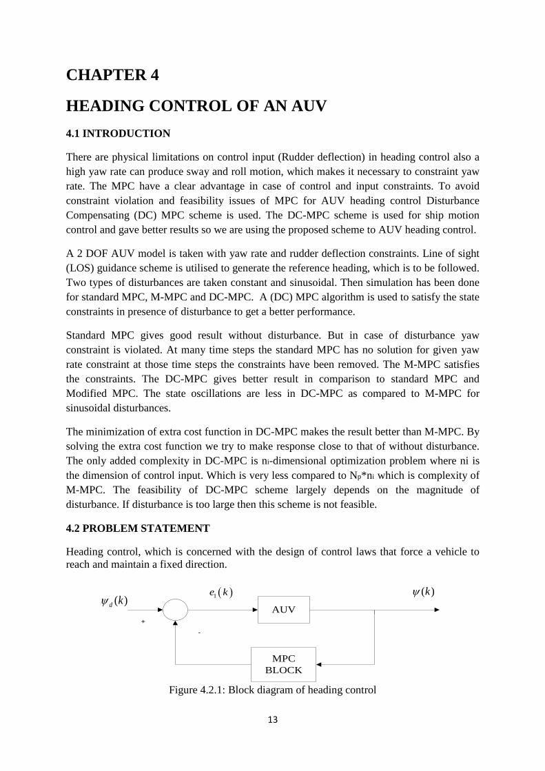
Heading control, which is concerned with the design of control laws that force a vehicle to reach and maintain a fixed direction.

AUV

MPC BLOCK

( )d kψ( )kψ( )1e k

+

-

Figure 4.2.1: Block diagram of heading control

13

Heading controller should give proper rudder angle to get force and moments required for the desired vehicle motion to correct yaw angle that caused by disturbances. The heading control system is actually a time-variant, high noise and nonlinear system. For this problem formulation following assumptions are made: I) It is assumed that AUV and target are on the same plane. II) The target stationary; however, targets can be considered non-stationary which is still

an area of active research. III) Navigation information is available to the guidance system.

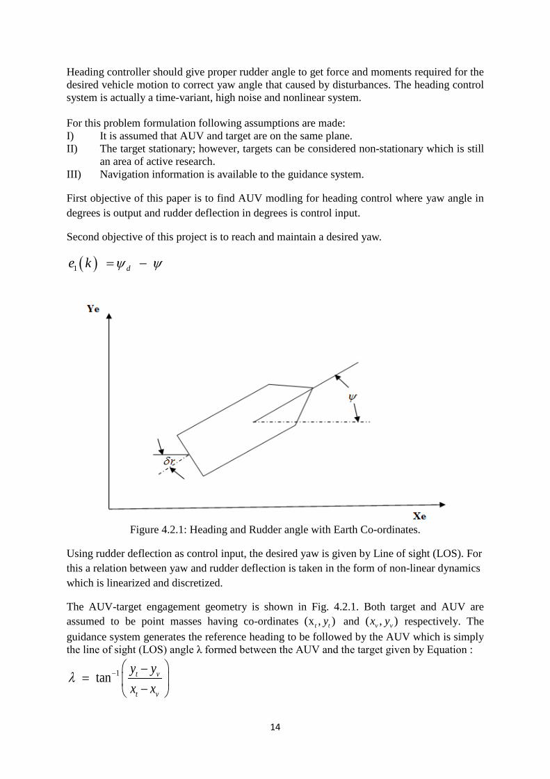
First objective of this paper is to find AUV modling for heading control where yaw angle in degrees is output and rudder deflection in degrees is control input.

Second objective of this project is to reach and maintain a desired yaw.

Figure 4.2.1: Heading and Rudder angle with Earth Co-ordinates.

Using rudder deflection as control input, the desired yaw is given by Line of sight (LOS). For this a relation between yaw and rudder deflection is taken in the form of non-linear dynamics which is linearized and discretized.

The AUV-target engagement geometry is shown in Fig. 4.2.1. Both target and AUV are assumed to be point masses having co-ordinates (x , )t ty and ( , )v vx y respectively. The guidance system generates the reference heading to be followed by the AUV which is simply the line of sight (LOS) angle λ formed between the AUV and the target given by Equation :

1tan t v

t v

y yx x

λ − −= −

( )1 de k ψ ψ= −

14

target

AUV reference

X

Y

λ

LOS

(x , )t ty

( , )v vx y

Figure 4.2.2: AUV-target engagement geometry

4.3 AUV MODELING

The kinematic equations of motion for an AUV on the horizontal X–Y plane can be written as:

cos sin 0sin cos 0

0 0 1

uy v

r

x ψ ψψ ψ

ψ

− =

Where, x and y represent the inertial coordinates of the CM of the vehicle and u and v are the surge and sway velocities in body fixed frame [3]. The orientation of the vehicle is described by the angle ψ measured from the inertial-X axis and r is its yaw (angular) velocity. Following assumptions are taken: (i) The CM coincides with the centre of buoyancy (CB), (ii) The mass distribution is homogeneous, (iii) The hydrodynamic drag terms of order more than two are neglected, and (iv) Angular orientations pitch and roll can be neglected. Now as we want to control only yaw by rudder movement we can neglect v. So, the kinematics will be

ucosX ψ=

usinY ψ=

15

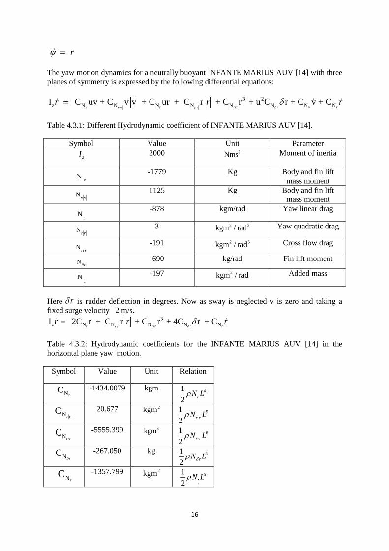
rψ = The yaw motion dynamics for a neutrally buoyant INFANTE MARIUS AUV [14] with three planes of symmetry is expressed by the following differential equations:

v r vv v

3 2z N N N N N N N NI C uv + C v v + C ur + C r + C r + u C r + C v + C

rrr r rr rr r r

δδ=

Table 4.3.1: Different Hydrodynamic coefficient of INFANTE MARIUS AUV [14].

Symbol Value Unit Parameter zI 2000 2Nms Moment of inertia

vN -1779 Kg Body and fin lift

mass moment

v vN 1125 Kg Body and fin lift

mass moment

rN -878 kgm/rad Yaw linear drag

N r r 3 2 2kgm / rad Yaw quadratic drag

N rrr -191 2 3kgm / rad Cross flow drag

N rδ -690 kg/rad Fin lift moment

.Nr

-197 2kgm / rad Added mass

Here rδ is rudder deflection in degrees. Now as sway is neglected v is zero and taking a fixed surge velocity 2 m/s.

r

3z N N N N NI 2C r + C r + C r + 4C r + C

rrr r rr rr r r

δδ=

Table 4.3.2: Hydrodynamic coefficients for the INFANTE MARIUS AUV [14] in the horizontal plane yaw motion.

Symbol Value Unit Relation

rNC -1434.0079 kgm 412 rN Lρ

NCr r

20.677 2kgm

512 r rN Lρ

NCrrr -5555.399 3kgm 61

2 rrrN Lρ

NCrδ

-267.050 kg 312 rN Lδρ

N Cr -1357.799 2kgm 51

2 rN Lρ •

16

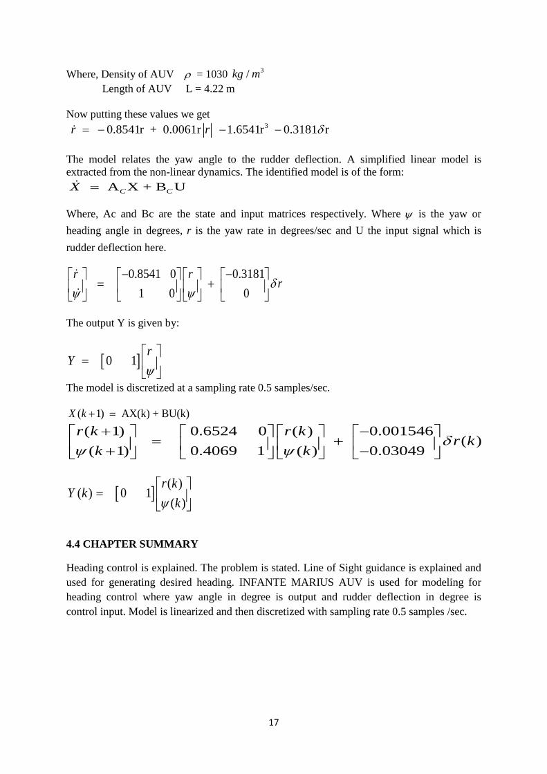
Where, Density of AUV ρ = 1030 3/kg m Length of AUV L = 4.22 m Now putting these values we get

30.8541r + 0.0061r 1.6541r 0.3181 rr r δ= − − −

The model relates the yaw angle to the rudder deflection. A simplified linear model is extracted from the non-linear dynamics. The identified model is of the form:

A X + B UC CX =

Where, Ac and Bc are the state and input matrices respectively. Where ψ is the yaw or heading angle in degrees, r is the yaw rate in degrees/sec and U the input signal which is rudder deflection here.

0.8541 0 0.31811 0 0

r rrδ

ψ ψ− −

= +

The output Y is given by:

[ ]0 1r

Yψ

=

The model is discretized at a sampling rate 0.5 samples/sec.

( 1) AX(k) + BU(k)X k + = ( 1) 0.6524 0 ( ) 0.001546

( )( 1) 0.4069 1 ( ) 0.03049

r k r kr k

k kδ

ψ ψ+ −

= + + −

[ ] ( )( ) 0 1

( )r k

Y kkψ

=

4.4 CHAPTER SUMMARY

Heading control is explained. The problem is stated. Line of Sight guidance is explained and used for generating desired heading. INFANTE MARIUS AUV is used for modeling for heading control where yaw angle in degree is output and rudder deflection in degree is control input. Model is linearized and then discretized with sampling rate 0.5 samples /sec.

17

CHAPTER 5

DESIGN OF MODEL PREDICTIVE CONTROL FOR AN AUV Consider a discrete-time linear time-invariant system with disturbances

( 1) 0.6524 0 ( ) 0.001546( ) ( )

( 1) 0.4069 1 ( ) 0.03049r k r k

r k w kk k

δψ ψ

+ − = + + + −

( 1) AX(k) + BU(k) + w(k) , wX k W+ = ∈

[ ] ( )( ) 0 1

( )r k

Y kkψ

=

( ) ( )Y k C X k=

Where w is unknown disturbance taking values in the set W.

5.1 DESIGN OF STANDARD MPC

The Standard MPC considers the following optimization problem

1

1 0( ) ( )

CP NNT T

S Sj i

J R Y Q R Y U R U−

= == − − + ∆ ∆∑ ∑

Subject to

( 1| ) ( | ) ( | )X k j k AX k j k BU k j k+ + = + + +

( | ) ( )X k k X k=

( 1| )cC X k j k D+ + ≤

( | )SU k j k T+ ≤

Where,

[ ( 1| ) ( 2 | ) ... ( | )]TPY y k k y k k y k N k= + + +

[ ( ) ( 1) ... ( 1)]TcU u k u k u k N∆ = ∆ ∆ + ∆ + − 18

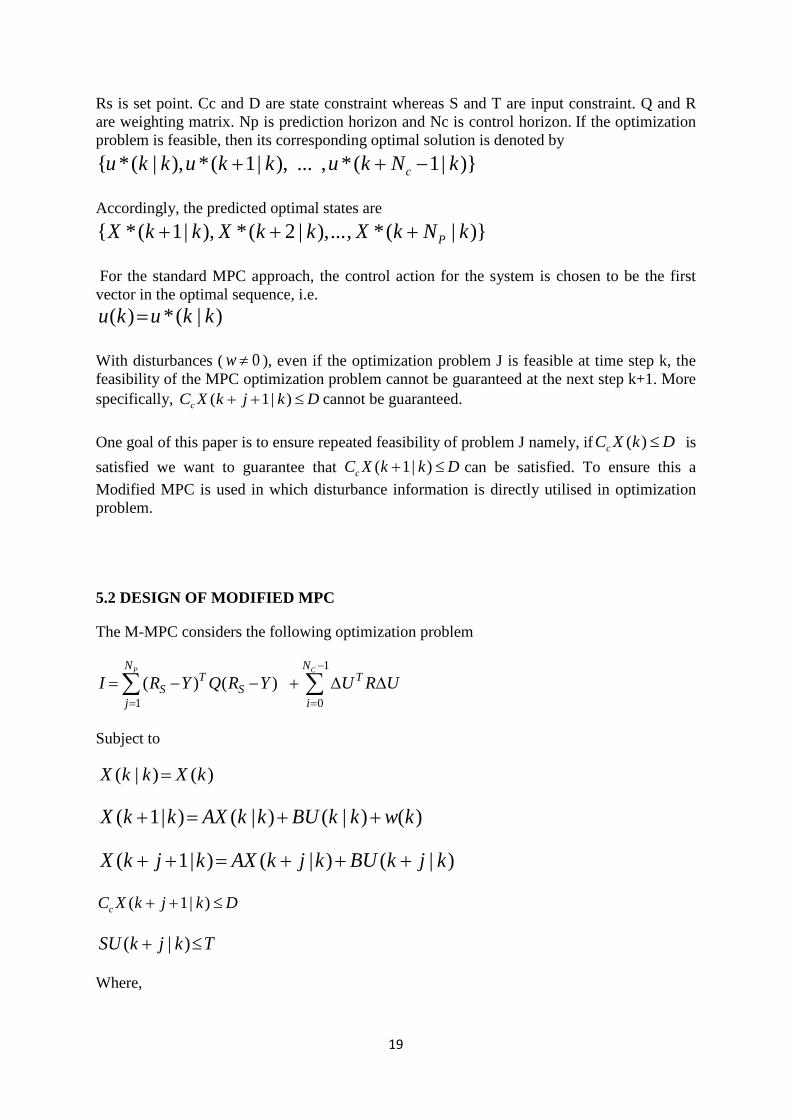
Rs is set point. Cc and D are state constraint whereas S and T are input constraint. Q and R are weighting matrix. Np is prediction horizon and Nc is control horizon. If the optimization problem is feasible, then its corresponding optimal solution is denoted by { *( | ), *( 1| ), ... , *( 1| )}cu k k u k k u k N k+ + − Accordingly, the predicted optimal states are { *( 1| ), *( 2 | ),..., *( | )}PX k k X k k X k N k+ + + For the standard MPC approach, the control action for the system is chosen to be the first vector in the optimal sequence, i.e.

( ) *( | )u k u k k= With disturbances ( 0w ≠ ), even if the optimization problem J is feasible at time step k, the feasibility of the MPC optimization problem cannot be guaranteed at the next step k+1. More specifically, ( 1| )cC X k j k D+ + ≤ cannot be guaranteed. One goal of this paper is to ensure repeated feasibility of problem J namely, if ( )cC X k D≤ is satisfied we want to guarantee that ( 1| )cC X k k D+ ≤ can be satisfied. To ensure this a Modified MPC is used in which disturbance information is directly utilised in optimization problem.

5.2 DESIGN OF MODIFIED MPC

The M-MPC considers the following optimization problem

1

1 0( ) ( )

CP NNT T

S Sj i

I R Y Q R Y U R U−

= == − − + ∆ ∆∑ ∑

Subject to

( | ) ( )X k k X k=

( 1| ) ( | ) ( | ) ( )X k k AX k k BU k k w k+ = + +

( 1| ) ( | ) ( | )X k j k AX k j k BU k j k+ + = + + +

( 1| )cC X k j k D+ + ≤

( | )SU k j k T+ ≤

Where,

19

[ ( 1| ) ( 2 | ) ... ( | )]TPY y k k y k k y k N k= + + +

[ ( ) ( 1) ... ( 1)]TcU u k u k u k N∆ = ∆ ∆ + ∆ + −

Cc and D are state constraint whereas S and T are input constraint. Q and R are weighting matrix. Np is prediction horizon and Nc is control horizon. If the optimization problem is feasible, then its corresponding optimal solution is denoted by { *( | ), *( 1| ), ... , *( 1| )}cu k k u k k u k N k+ + − Accordingly, the predicted optimal states are { *( 1| ), *( 2 | ),..., *( | )}PX k k X k k X k N k+ + + For the M-MPC approach, the control action for the system is chosen to be the first vector in the optimal sequence, i.e.

( ) *( | )u k u k k= Using the M-MPC scheme, the state constraints normally can be satisfied.

5.3 DESIGN OF DISTURBANCE COMPENSATED MPC

Using the M-MPC scheme, the state constraints normally can be satisfied. However, the system performance is not satisfactory for heading control. To improve the system responses, the DC-MPC scheme is proposed to not only satisfy the state constraints in the presence of disturbance, but also to retain the performance level achieved by the system in calm water (without disturbance). The design of the DC-MPC involves several steps as described below.

Step 1: At time step k, calculate the disturbance ( 1)kwΛ

− of the previous time step using,

( 1) ( ) ( 1) ( 1)k x k Ax k Bu kwΛ

− = − − − − Step 2: Calculate the disturbance compensation control u∆ by solving the optimization problem

min ( 1)u

I CB u C w kΛ

∆= ∆ + −

Subject to

( 1)CB u C w kΛ

∆ ≤− −

S u T∆ ≤ Step 3: Solve the following optimization problem

20

1

1 0( ) ( )

CP NNT T

S Sj i

J R Y Q R Y U R U−

= == − − + ∆ ∆∑ ∑

Subject to

( 1| ) ( | ) ( | )X k j k AX k j k BU k j k+ + = + + +

( | ) ( )X k k X k=

( 1| )cC X k j k D+ + ≤

( | )Su k k T S u≤ − ∆ ∗

( | )SU k j k T+ ≤

Where,

[ ( 1| ) ( 2 | ) ... ( | )]TPY y k k y k k y k N k= + + +

[ ( ) ( 1) ... ( 1)]TcU u k u k u k N∆ = ∆ ∆ + ∆ + −

Rs is set point. Cc and D are state constraint whereas S and T are input constraint. Q and R are weighting matrix. Np is prediction horizon and Nc is control horizon. If the optimization problem is feasible, then its corresponding optimal solution is denoted by { *( | ), *( 1| ), ... , *( 1| )}cu k k u k k u k N k+ + − Accordingly, the predicted optimal states are { *( 1| ), *( 2 | ),..., *( | )}PX k k X k k X k N k+ + + For the standard MPC approach, the control action for the system is chosen to be the first vector in the optimal sequence, i.e.,

( ) *( | )u k u k k=

Step 4: The following control is implemented to the system

( ) ( | )u k u k k u= ∗ + ∆ ∗

21

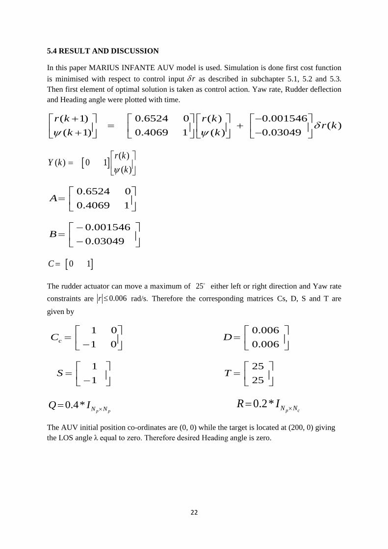
5.4 RESULT AND DISCUSSION

In this paper MARIUS INFANTE AUV model is used. Simulation is done first cost function is minimised with respect to control input rδ as described in subchapter 5.1, 5.2 and 5.3. Then first element of optimal solution is taken as control action. Yaw rate, Rudder deflection and Heading angle were plotted with time.

( 1) 0.6524 0 ( ) 0.001546( )

( 1) 0.4069 1 ( ) 0.03049r k r k

r kk k

δψ ψ

+ − = + + −

[ ] ( )( ) 0 1

( )r k

Y kkψ

=

0.6524 00.4069 1

A =

0.0015460.03049

B−

= −

[ ]0 1C =

The rudder actuator can move a maximum of 25 either left or right direction and Yaw rate constraints are 0.006r ≤ rad/s. Therefore the corresponding matrices Cs, D, S and T are

given by

1 01 0cC

= −

0.0060.006

D =

11

S = −

2525

T =

0.4*p pN NQ I ×= 0.2*

p cN NR I ×=

The AUV initial position co-ordinates are (0, 0) while the target is located at (200, 0) giving the LOS angle λ equal to zero. Therefore desired Heading angle is zero.

22

1. STANDARD MPC

Two disturbances are considered in this case. One is constant disturbance (-0.0015) and other is sinusoidal disturbance (0.001sin (0.08t)). Np =80 and Nc = 80 are chosen. The parameters are chosen to achieve good performance in calm water. Figure shows that although the standard MPC scheme achieves good performance in calm water in terms of meeting constraints and achieving desired heading, the performance of the standard MPC in the presence of disturbances is not satisfactory. The yaw constraint violations are observed with both constant and sinusoidal disturbances.

Figure 5.4.1: Yaw rate (rad/sec) vs. Time (sec) for standard MPC

AUV heading when MPC is applied which clearly shows that LOS is closely followed by UV. Initial yaw angle is 30 degree.

Figure 5.4.2: Heading angle (deg) vs. Time (sec) for standard MPC

0 25 50 75 100 125 150 175 200 225 250-8

-6

-4

-2

0

2

4

6

8x 10-3

Time(sec)

Yaw

Vel

ocity

(rad

/sec

)

No DisturbanceConstant DisturbanceSinusoidal Disturbance

Yaw Constraint

0 25 50 75 100 125 150 175 200 225 250-30

-20

-10

0

10

20

30

Time (sec)

Hea

ding

Ang

le (d

eg)

No DisturbanceConstant DisturbanceSinusoidal Disturbance

23

The controller output (rudder deflections) needed to track the LOS is within the constrained limits of rudder actuator.

Figure 5.4.3: Rudder angle (deg) vs. Time (sec) for standard MPC

2. M-MPC WITH CONSTANT DISTURBANCE

Simulation is done with constant disturbances but with different Np and Nc values. The Yaw constraints are successfully enforced by M-MPC.

Figure 5.4.4: Yaw rate (rad/sec) vs. Time (sec) for M-MPC with constant disturbance

Figure 5.4.5: Heading angle (deg) vs. Time (sec) for M-MPC with constant disturbance

0 25 50 75 100 125 150 175 200 225 250-30

-20

-10

0

10

20

30

Time (sec)

Rud

der A

ngle

(Deg

ree)

No DisturbanceConstant DisturbanceSinusoidal Disturbance

0 25 50 75 100 125 150 175 200 225 250

-6

-4

-2

0

2

4

6

x 10-3

Time (sec)

Yaw

Velo

city

(rad/

sec)

Prediction Step = 8Prediction Step = 20Prediction Step = 80

0 25 50 75 100 125 150 175 200 225 250-30

-20

-10

0

10

20

30

Time (sec)

Hea

ding

ang

le (d

eg)

Prediction Step = 8Prediction Step = 20Prediction Step = 80

24

Figure 5.4.6: Rudder angle (deg) vs. Time (sec) for M-MPC with constant disturbance

3. M-MPC WITH SINUSOIDAL DISTURBANCE

With sinusoidal disturbances the results are given below. Again Yaw rate constraint is satisfied.

Figure 5.4.7: Yaw rate (rad/sec) vs. Time (sec) for M-MPC with sinusoidal disturbance

Figure 5.4.8: Heading angle (deg) vs. Time (sec) for M-MPC with sinusoidal disturbance

0 25 50 75 100 125 150 175 200 225 250-30

-20

-10

0

10

20

30

Time (sec)

Rud

der A

ngle

(deg

)

Prediction Step = 8Prediction Step = 20Prediction Step = 80

0 25 50 75 100 125 150 175 200 225 250

-6

-4

-2

0

2

4

6

x 10-3

Time (sec)

Yaw

Vel

ocity

(rad

/sec

)

Prediction Step = 8Prediction Step = 20Prediction Step = 80

0 25 50 75 100 125 150 175 200 225 250-30

-20

-10

0

10

20

30

Time (sec)

Hea

ding

Ang

le (d

eg)

Prediction Step = 8Prediction Step = 20Prediction Step = 80

25

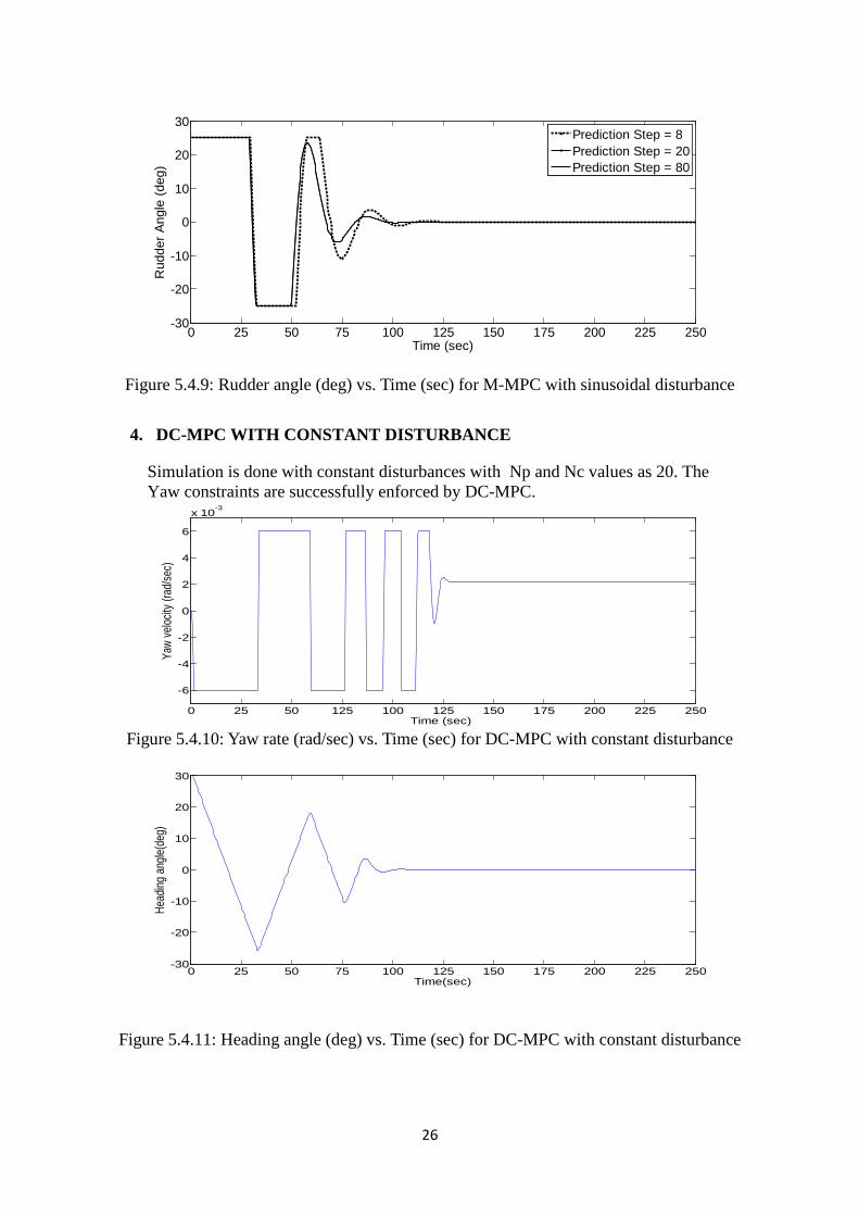
Figure 5.4.9: Rudder angle (deg) vs. Time (sec) for M-MPC with sinusoidal disturbance

4. DC-MPC WITH CONSTANT DISTURBANCE

Simulation is done with constant disturbances with Np and Nc values as 20. The Yaw constraints are successfully enforced by DC-MPC.

Figure 5.4.10: Yaw rate (rad/sec) vs. Time (sec) for DC-MPC with constant disturbance

Figure 5.4.11: Heading angle (deg) vs. Time (sec) for DC-MPC with constant disturbance

0 25 50 75 100 125 150 175 200 225 250-30

-20

-10

0

10

20

30

Time (sec)

Rud

der A

ngle

(deg

)

Prediction Step = 8Prediction Step = 20Prediction Step = 80

0 25 50 125 100 125 150 175 200 225 250

-6

-4

-2

0

2

4

6

x 10-3

Time (sec)

Yaw

veloc

ity (r

ad/se

c)

0 25 50 75 100 125 150 175 200 225 250-30

-20

-10

0

10

20

30

Time(sec)

Head

ing an

gle(d

eg)

26

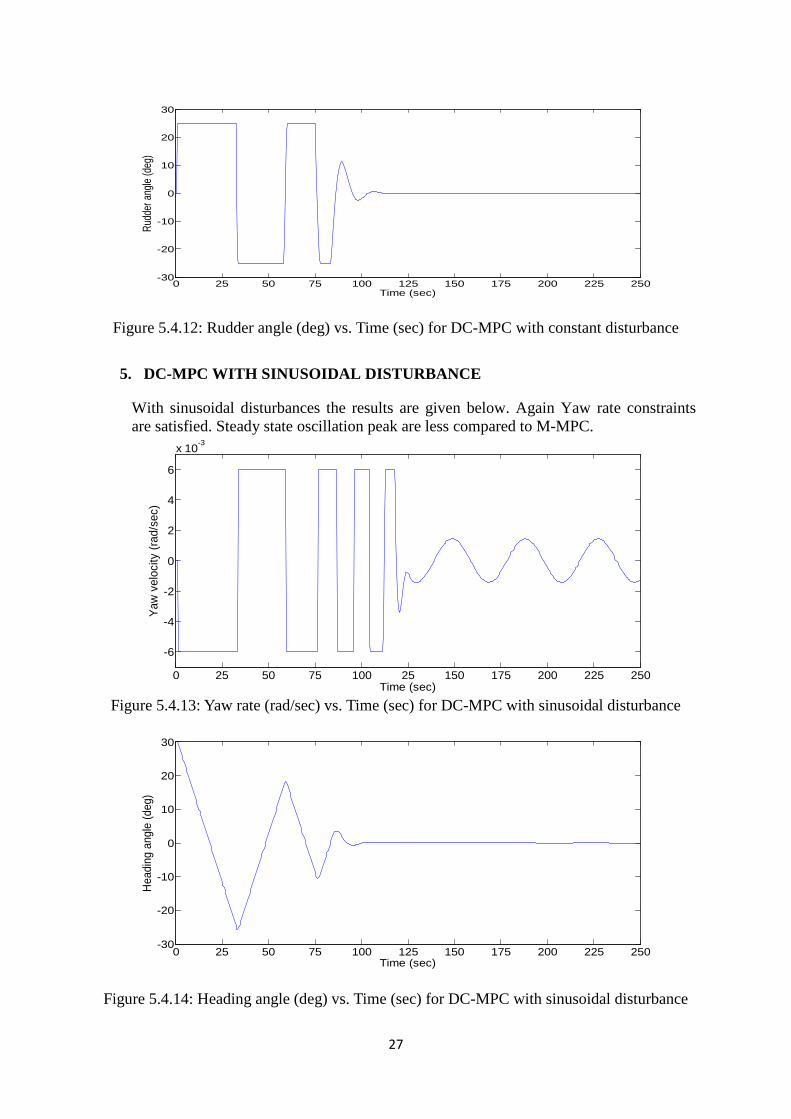
Figure 5.4.12: Rudder angle (deg) vs. Time (sec) for DC-MPC with constant disturbance

5. DC-MPC WITH SINUSOIDAL DISTURBANCE

With sinusoidal disturbances the results are given below. Again Yaw rate constraints are satisfied. Steady state oscillation peak are less compared to M-MPC.

Figure 5.4.13: Yaw rate (rad/sec) vs. Time (sec) for DC-MPC with sinusoidal disturbance

Figure 5.4.14: Heading angle (deg) vs. Time (sec) for DC-MPC with sinusoidal disturbance

0 25 50 75 100 125 150 175 200 225 250-30

-20

-10

0

10

20

30

Time (sec)

Rudd

er an

gle (d

eg)

0 25 50 75 100 25 150 175 200 225 250

-6

-4

-2

0

2

4

6

x 10-3

Time (sec)

Yaw

vel

ocity

(rad

/sec

)

0 25 50 75 100 125 150 175 200 225 250-30

-20

-10

0

10

20

30

Time (sec)

Hea

ding

ang

le (d

eg)

27

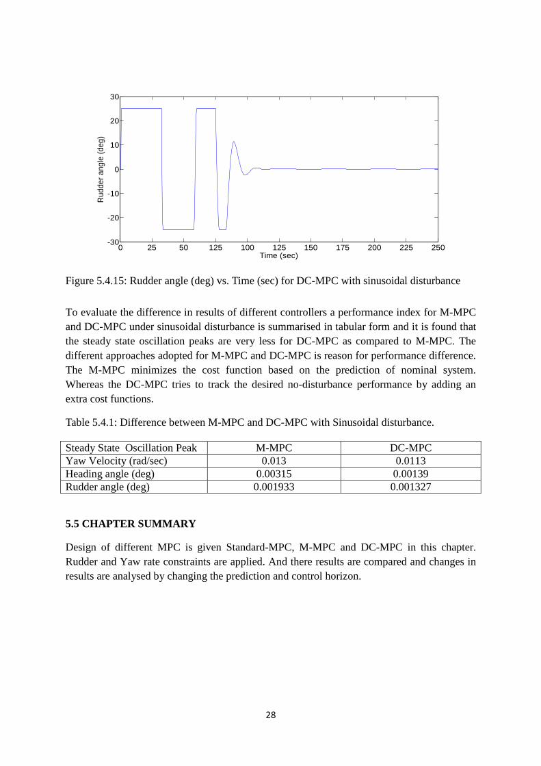
Figure 5.4.15: Rudder angle (deg) vs. Time (sec) for DC-MPC with sinusoidal disturbance

To evaluate the difference in results of different controllers a performance index for M-MPC and DC-MPC under sinusoidal disturbance is summarised in tabular form and it is found that the steady state oscillation peaks are very less for DC-MPC as compared to M-MPC. The different approaches adopted for M-MPC and DC-MPC is reason for performance difference. The M-MPC minimizes the cost function based on the prediction of nominal system. Whereas the DC-MPC tries to track the desired no-disturbance performance by adding an extra cost functions.

Table 5.4.1: Difference between M-MPC and DC-MPC with Sinusoidal disturbance.

Steady State Oscillation Peak M-MPC DC-MPC Yaw Velocity (rad/sec) 0.013 0.0113 Heading angle (deg) 0.00315 0.00139 Rudder angle (deg) 0.001933 0.001327

5.5 CHAPTER SUMMARY

Design of different MPC is given Standard-MPC, M-MPC and DC-MPC in this chapter. Rudder and Yaw rate constraints are applied. And there results are compared and changes in results are analysed by changing the prediction and control horizon.

0 25 50 125 100 125 150 175 200 225 250-30

-20

-10

0

10

20

30

Time (sec)

Rud

der a

ngle

(deg

)

28

CHAPTER 6

CONCLUSIONS & SUGGESTIONS FOR FUTURE WORK 6.1 CONCLUSIONS Yaw angle of an AUV is controlled by rudder deflection using MPC. The simple line of sight (LOS) guidance scheme is used to generate the reference heading. The results given are for stationary targets. In standard MPC the Yaw rate constraint violations are observed in the presence of disturbance. While in M-MPC yaw rate constraints are satisfied. DC-MPC satisfies the state constraints as well as gives better performance as compared to M-MPC. It reduces the state and control oscillations. DC-MPC need less computation as compared to robust MPC. All objectives are achieved using DC-MPC the results with disturbance are close to standard- MPC results without disturbance. 6.2 CONTRIBUTION

The following are contributions of the thesis: • In Position Control the variation in output is analysed by varying control interval of

MPC. • In Heading Control results of various MPC techniques are compared. • The steady state errors in Heading Control are reduced using DC-MPC.

6.3 SUGGESTIONS FOR FUTURE WORK

After this further work will be designing Robust MPC for heading control and compare the added complexity and change in performance. Robust MPC is used for various control problems of AUV it is used when we consider uncertainty in model and noise. In this the plant model and the model used to predict future state are different. An extra unmeasured disturbance is added to the model.

29

REFRENCES

[1] Blidberg, D Richard. “The Development of Autonomous Underwater Vehicles (AUV); A Brief Summary”. Autonomous Undersea Systems Institute, Lee New Hampshire, USA.

[2] E. Desa, R. Madhan and P. Maurya, “Potential of autonomous underwater vehicles as new generation ocean data platforms”. National Institute of Oceanography, Dona Paula, Goa, India.

[3] T. Fossen, Guidance and Control of Ocean Vehicles. Wiley, New York 1994.

[4] Clarke, D. W., C. Mohtadi and P. S. Tuff (1987a). Generalized predictive control. Part 1: The basic algorithm. Automatica, vol. 23, no. 2, pp. 137- 148.

[5] Clarke, D. W., C. Mohtadi and P. S. Tuff (1987b). Generalized predictive control.

Part 2: Extensions and Interpretations. Automatica, vol. 23, no. 2, pp. 149-160. [6] T. Fossen, “Marine Control Systems, ”Marine Cybernetics, Trondheim, Norway,

2002.

[7] S. Qin and T. Badgwell, “A survey of industrial model predictive control technology,” Control Eng. Practice, vol. 11, pp. 733–764, 2003.

[8] J. Rawlings and D. Mayne, Model Predictive Control Theory and Design. Madison,

WI: Nob Hill Publishing, 2009 [9] E. Gilbert, I. Kolmanovsky, and K. Tan, “Discrete-time reference governors and the

nonlinear control of systems with state and control constraints,” Int. J. Robust Nonlinear Control, vol. 5, pp. 487–504, 1995.

[10] A.Wahl and E. Gilles, “Track-keeping on waterways using model predictive control,”

in Proc. IFAC Conf. Control Appl. Marine Syst., 1998, pp. 149–154. [11] T. Perez, C. Tzeng, and G. Goodwin, “Model predictive rudder roll stabilization

control for ships,” presented at the 5th IFAC Conf. Maneuvering Control Marine Craft, Aalborg, Denmark, 2000.

[12] Z. Li, J. Sun, and S. Oh, “Path following for marine surface vessels with rudder and

roll constraints: An MPC approach,” in Proc. Amer. Control Conf., 2009, pp. 3611–3616.

[13] P. Scokaert and J. Rawlings, “Feasibility issues in linear model predictive control,”

Amer. Inst. Chem. Eng. J., vol. 45, no. 8, pp. 1649–1659, 1999. [14] C. Silvestre, A. Pascoal (2004). ” Control of the INFANTE AUV using Gain

scheduled static output feedback.” Elsevier Control Engg Practice 12 (2004), pages 1501-1509.

30

[15] Ji-Hong Li, Pan-Mook Lee, “Design of an adaptive nonlinear controller for depth control of an autonomous underwater vehicle” Ocean Engineering Volume 32, Issues 17–18, December 2005, Pages 2165–2181.

[16] Zhen Li, Jing Sun, 2010, “Disturbance Compensating MPC with application to Ship Heading Control”. IEEE Trans. Control Sys. Tech., Vol. 20, No. 1, pp. 257-265.

[17] Liuping Wang, “ Model Predictive Control System Design and Implementation Using MATLAB”, Springer, Advances in industrial control, 2009.

[18] Garcia, C. E., Prett, D. M., & Morari, M. (1989). ” Model predictive control: theory and practice -a survey” Automatica, Vol. 25(3), pages 335-348.

[19] D. Mayne, J. Rawlings, C. Rao, and P. Scokaert, “Constrained model predictive control: Stability and optimality,” Automatica, vol. 36, pp.789–814, 2000.

[20] A. Zheng and M. Morari, “Robust stability of constrained model predictive control,” in Proc. Amer. Control Conf., 1993, pp. 379–383.

[21] P. Scokaert and D. Mayne, “Min-max feedback model predictive control for constrained linear systems,” IEEE Trans. Autom. Control, vol. 43, no. 8, pp. 1136–1142, Aug. 1998.

[22] L. Chisci, J. Rossiter, and G. Zappa, “Systems with persistent disturbances: Predictive control with restrictive constraints,” Automatica, vol. 37, pp. 1019–1028, 2001.

[23] Y. Lee and B. Kouvaritakis, “Robust receding control for systems with uncertain dynamics and input saturation,” Automatica, vol. 36, pp. 1497–1504, 2000.

[24] D. Mayne, M. Seron, and S. Rakovic, “Robust model predictive control of constrained linear systems with bounded disturbances,” Automatica, vol. 41, pp. 1136–1142, 2005.

[25] R. Ghaemi, J. Sun, and I. Kolmanovsky, “Computationally efficient model predictive control with explicit disturbance mitigation and constraint enforcement,” in Proc. 45th IEEE Conf. Decision Control, 2006, pp. 4842–4847.

[26] Z. Li, J. Sun, and R. Beck, “Evaluation and modification of a robust path following controller for marine surface vessels in wave fields,” J.

31