Portfolio analysis - Excel and VBAexcelatfinance.com/xlf/xlf-portfolio-v2.pdf · Covariance with...

Portfolio Analysis

© Copyright: Dr Ian O’Connor, CPA excelatfinance.com of 16

PORTFOLIO ANALYSIS

A portfolio can be viewed as a combination of assets held by an investor. For each asset held, such as company stocks, the logarithmic or continuously compounded rate of return r at time t is given by

�� = ��

where � is the stock price at time t, and �� is the stock price in the prior period.

The volatility of stock returns, over period N is often estimated by the sample variance �

σ� =�� − �̅�� − 1

�

��

where r� is the return realized in period t, and N is the number of time intervals. As the variance of returns is in units of percent squared, we take the square root to determine the standard deviation .

Example (file: xlf-portfolio-analysis-v2.xlsm)

Suppose an investor has a four stock portfolio comprising of shares on the Australian stock market as listed in Figure 1.

Fig 1: Excel functions - descriptive statistics

The stock codes AGK, CSL, SPN, and SKT from figure 1 are described in figure 2.

Portfolio Analysis


Fig 2: Portfolio components - description

1. Descriptive statistics

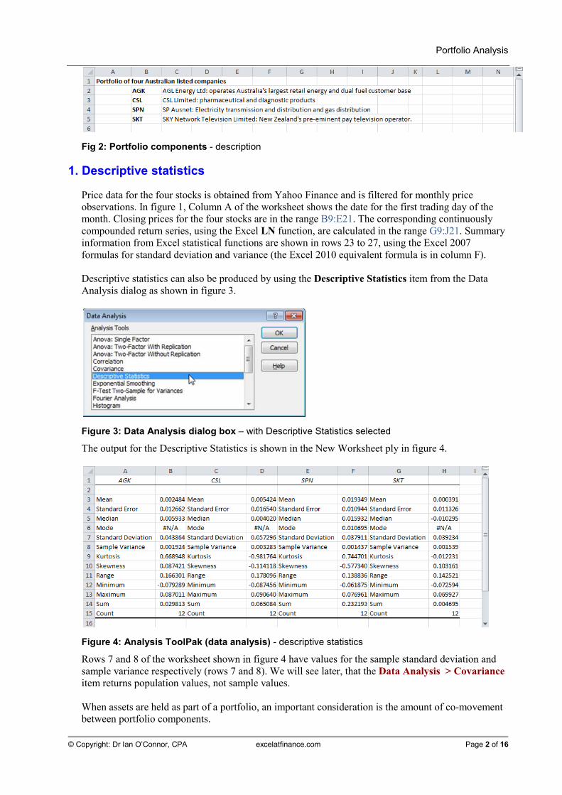
Price data for the four stocks is obtained from Yahoo Finance and is filtered for monthly price observations. In figure 1, Column A of the worksheet shows the date for the first trading day of the month. Closing prices for the four stocks are in the range B9:E21. The corresponding continuously compounded return series, using the Excel LN function, are calculated in the range G9:J21. Summary information from Excel statistical functions are shown in rows 23 to 27, using the Excel 2007 formulas for standard deviation and variance (the Excel 2010 equivalent formula is in column F). Descriptive statistics can also be produced by using the Descriptive Statistics item from the Data Analysis dialog as shown in figure 3.

Figure 3: Data Analysis dialog box – with Descriptive Statistics selected

The output for the Descriptive Statistics is shown in the New Worksheet ply in figure 4.

Figure 4: Analysis ToolPak (data analysis) - descriptive statistics

Rows 7 and 8 of the worksheet shown in figure 4 have values for the sample standard deviation and sample variance respectively (rows 7 and 8). We will see later, that the Data Analysis > Covariance item returns population values, not sample values. When assets are held as part of a portfolio, an important consideration is the amount of co-movement between portfolio components.

Portfolio Analysis


2. Covariance

The amount of co-movement can be measured by the covariance statistic, and is calculated on a pair-

wise basis. The formula for the sample covariance �,� for the return vectors of stock i and stock j is

�,� =��,� − �� !��,� − �" !� − 1

�

��

There are number of ways the estimation can be operationalized and some techniques are described in this section. Methods include the Analysis ToolPak – Covariance item (figure 3), and Excel functions listed here.

Excel 2007

COVAR(array1,array2) Returns covariance, the average of the products of paired deviations

Excel 2010

COVARIANCE.S(array1,array2) Returns the sample covariance, the average of the products deviations for each data point pair in two data sets

COVARIANCE.P(array1,array2) Returns covariance, the average of the products of paired deviations

The worksheet in figure 7 shows output for the Analysis ToolPak (ATP) covariance item in rows 32 to 36. The covariance matrix, from the ATP is a lower triangular table, meaning it only returns the main diagonal elements, and the lower left elements. By definition, the covariance of a vector with

itself, is the variance of the vector. Thus, the value in cell G33 in figure 5, #$%,#$% = 0.001764, is the same value as the population variance returned by the Excel VARP function shown in figure 1 cell G28.

Fig 5: Variance covariance matrix - ATP and COVAR versions

In Excel 2007 and earlier, there is only one covariance function, COVAR and it returns the population covariance for two return vectors. In figure 5, rows 39 to 43, the COVAR function uses Excel range names for each of the return vectors. The return values are population estimates. Construction of the individual cell formulas can be simplified by using range names with the INDIRECT function. To do this:

• Copy and paste the stock codes vector to the range G46:J46.

• Using Paste Special > Transpose, paste the transposed stock codes vector to F47.

Portfolio Analysis


• Enter the formula =COVAR(INDIRECT(F$47),INDIRECT($G46)) at G47.

• Copy and paste the formula to complete the variance covariance matrix.

The return values, and cell formulae are shown in figure 6.

Fig 6: Variance covariance matrix - COVAR and INDIRECT version

3. Covariance with VBA

The Excel 2007 COVAR function returns the population covariance. To estimate the sample covariance, the custom function Covar_s has been developed. Here is the code.

VBA: Covar_s (Available in the XLFProject.XLF_Module)

10 20 30 40 50 60 70 80 90 100

Function Covar_s(InArray1 As Variant, InArray2 As Variant) As Variant Dim NumRows As Long, NumRows1 As Long, NoRows2 As Long Dim i As Long, j As Long Dim InArrayType1 As String Dim InArrayType2 As String Dim InA1Ave As Double, InA2Ave As Double Dim Temp1() As Double, Temp2 As Double On Error GoTo ErrHandler InArrayType1 = TypeName(InArray1) InArrayType2 = TypeName(InArray2) If InArrayType1 = "Range" Then NumRows = UBound(InArray1.Value2, 1) - _ LBound(InArray1.Value2, 1) + 1 ElseIf InArrayType1 = "Variant()" Then NumRows = UBound(InArray1, 1) - LBound(InArray1, 1) + 1 Else GoTo ErrHandler End If

Portfolio Analysis


110 120 130 140 150 160 170 180 190 200 210 220

ReDim Temp1(1 To NumRows) With Application.WorksheetFunction InA1Ave = .Average(InArray1) InA2Ave = .Average(InArray2) For i = 1 To NumRows Temp1(i) = (InArray1(i) - InA1Ave) * (InArray2(i) - InA2Ave) Next i Temp2 = .Sum(Temp1) / (NumRows – 1) End With Covar_s = Temp2 Exit Function ErrHandler: Covar_s = CVErr(xlErrNA) End Function

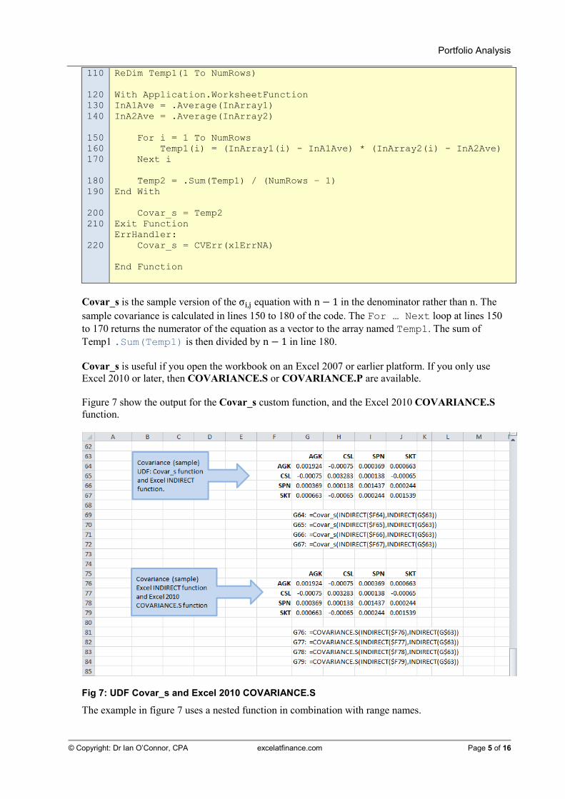
Covar_s is the sample version of the σ+,, equation with n − 1 in the denominator rather than n. The

sample covariance is calculated in lines 150 to 180 of the code. The For … Next loop at lines 150

to 170 returns the numerator of the equation as a vector to the array named Temp1. The sum of

Temp1 .Sum(Temp1) is then divided by n − 1 in line 180. Covar_s is useful if you open the workbook on an Excel 2007 or earlier platform. If you only use Excel 2010 or later, then COVARIANCE.S or COVARIANCE.P are available. Figure 7 show the output for the Covar_s custom function, and the Excel 2010 COVARIANCE.S function.

Fig 7: UDF Covar_s and Excel 2010 COVARIANCE.S

The example in figure 7 uses a nested function in combination with range names.

Portfolio Analysis


The next code section provides a custom function to return the variance-covariance as a single array formula. It uses the Excel 2007 COVAR function, for the population covariance, at line 170,butthecode is easily modified. The function is named VarCovar_p and is entered as an array CSE formula.

VBA: VarCovar_p (Available in the XLFProject.XLF_Module)

10 20 30 40 50 60 70 80 90 100 110 120 130 140 150 160 170 180 190 200 210 220 230

Function VarCovar_p(InMatrix As Variant) As Variant Dim NumRows As Long, numCols As Long Dim i As Long, j As Long Dim InMatrixType As String Dim Temp() As Double On Error GoTo ErrHandler InMatrixType = TypeName(InMatrix) If InMatrixType = "Range" Then NumRows = UBound(InMatrix.Value2, 1) - _ LBound(InMatrix.Value2, 1) + 1 numCols = UBound(InMatrix.Value2, 2) - _ LBound(InMatrix.Value2, 2) + 1 ReDim Temp(1 To numCols, 1 To numCols) ElseIf InMatrixType = "Variant()" Then NumRows = UBound(InMatrix, 1) - LBound(InMatrix, 1) + 1 numCols = UBound(InMatrix, 2) - LBound(InMatrix, 2) + 1 ReDim Temp(1 To numCols, 1 To numCols) Else GoTo ErrHandler End If With Application.WorksheetFunction For i = 1 To numCols For j = 1 To numCols Temp(i, j) = .Covar(.Index(InMatrix, 0, i), _ .Index(InMatrix, 0, j)) Next j Next i End With VarCovar_p = Temp Exit Function ErrHandler: VarCovar_p = CVErr(xlErrNA) End Function

To use VarCovar_p function do the following:

• Determine the dimensions of the returned variance-covariance (VCV) matrix.

• Give the returns data at G9:J21 a name, such as Returns.

• Select the range where the result is to be returned to.

• In the formula bar enter =VarCovar_p(Returns)

• Hit Control+Shift+Enter to complete the array formula.

• Add labels as shown in figure 5.

Portfolio Analysis


Fig 8: User defined array function - VarCovar_p

In the next section we examine the correlation coefficient.

4. Correlation

Correlation is a standardized measure of co-movement. The formula to calculate the correlation 3�,� between the returns for stocks i and j is

3�,� = �,� � �

where �,� is the covariance, and � and � are the standard deviation, and stocks i and j respectively. The Excel function is CORREL.

Excel

CORREL(array1,array2) Returns the correlation coefficient between two data sets

The correlation coefficient 3 is bounded in the range −1 ≤ 3�,� ≤ 1 . A correlation of -1 is perfect negative correlation, a correlation of +1 is perfect positive correlation, and a correlation of 0 represents zero correlation.

Fig 9: Correlation matrix - for the four stock portfolio

Portfolio Analysis


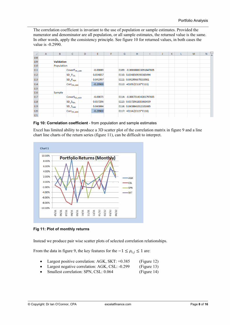
The correlation coefficient is invariant to the use of population or sample estimates. Provided the numerator and denominator are all population, or all sample estimates, the returned value is the same. In other words, apply the consistency principle. See figure 10 for returned values, in both cases the value is -0.2990.

Fig 10: Correlation coefficient - from population and sample estimates

Excel has limited ability to produce a 3D scatter plot of the correlation matrix in figure 9 and a line chart line charts of the return series (figure 11), can be difficult to interpret.

Fig 11: Plot of monthly returns

Instead we produce pair wise scatter plots of selected correlation relationships.

From the data in figure 9, the key features for the −1 ≤ 3�,� ≤ 1 are:

• Largest positive correlation: AGK, SKT: +0.385 (Figure 12)

• Largest negative correlation: AGK, CSL: -0.299 (Figure 13)

• Smallest correlation: SPN, CSL: 0.064 (Figure 14)

Portfolio Analysis


Figure 12: Largest positive correlation: AGK, SKT: +0.385

The positive correlation for AGK, SKT is shown by the positive (upward) slope of linear trend line in figure 12. In contrast, the negative correlation between the returns for AGK and CSL is shown by the negative (downward) slope of the linear trend line (figure 13)

Fig 13: Largest negative correlation - AGK, CSL: -0.299

In the case where the correlation is close to zero, then the linear trend line is more flat, as shown in figure 14.

Portfolio Analysis


Figure 14: Smallest correlation: SPN, CSL: 0.064

5. The portfolio

The returns �5 on a portfolio are the weight sum of the returns for the individual assets

�5 =�6��7

��

If the investor has portfolio weights of 8 = 0.1, 9 = 0.2, ; = 0.4, < = 0.3, then the portfolio return is shown in figure 15.

Fig 15: Portfolio returns

In figure 15, portfolio returns are estimated using the formula, line 10. The Excel SUMPRODUCT function is in row 12, and array formulae, are in rows 11 and 13. Both require Control+Shift+Enter.

The variance of the returns σ5� on a portfolio are estimated by the double summation formula

Portfolio Analysis


σ>� =��6�6� �,�7

��

7

��

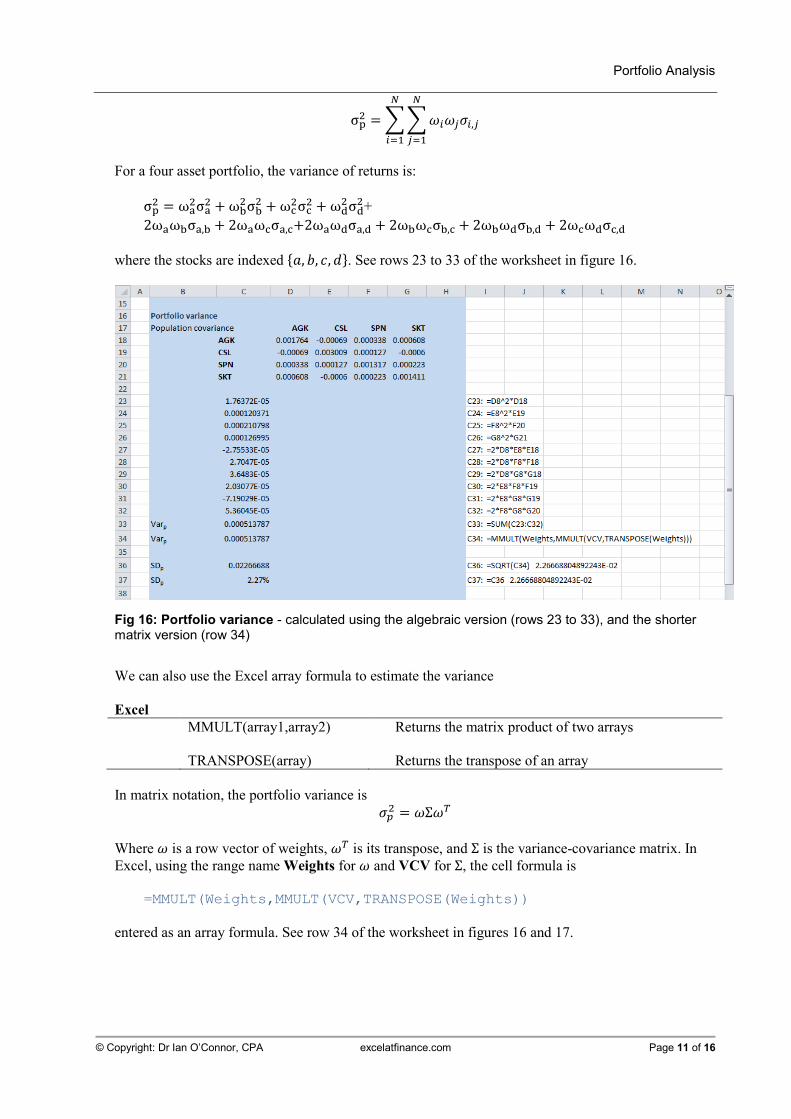
For a four asset portfolio, the variance of returns is:

σ>� = ω@�σ@� +ωB�σB� +ωC�σC� +ωD�σD�+ 2ω@ωBσ@,B + 2ω@ωCσ@,C+2ω@ωDσ@,D + 2ωBωCσB,C + 2ωBωDσB,D + 2ωCωDσC,D

where the stocks are indexed E8, 9, ;, <F. See rows 23 to 33 of the worksheet in figure 16.

Fig 16: Portfolio variance - calculated using the algebraic version (rows 23 to 33), and the shorter matrix version (row 34)

We can also use the Excel array formula to estimate the variance Excel

MMULT(array1,array2) Returns the matrix product of two arrays

TRANSPOSE(array) Returns the transpose of an array

In matrix notation, the portfolio variance is

5� = 6Σ6H

Where 6 is a row vector of weights, 6H is its transpose, and Σ is the variance-covariance matrix. In

Excel, using the range name Weights for 6 and VCV for Σ, the cell formula is

=MMULT(Weights,MMULT(VCV,TRANSPOSE(Weights)) entered as an array formula. See row 34 of the worksheet in figures 16 and 17.

Portfolio Analysis


Fig 17: Portfolio variance in Excel function format.

Portfolio Analysis


6. Portfolio charts

The x-y scatter plot of the portfolio and components is shown in figure 18. The figure indicates that the return for SPN is almost four times greater than the other components. Due to the covariance structure, the standard deviation of portfolio is lower than the standard deviation of any of the component stocks. In the next section we describe a method to rebalance the portfolio, in the case where the investor wants to achieve a different risk return tradeoff.

Fig 18: Portfolio and components

7. Portfolio optimization

Target 1: Suppose that the investor wants to rebalance the portfolio to achieve a target return of 1.5% per month with the lowest possible standard deviation. The investor assumes that the historical information can be used as an estimate of expected returns and risk in the future. In addition bounds are set on the proportion of funds in each stock. The weights in the individual stocks AGK, CSL, and SPN must be in the range 10% to 30%, the weight in SKT must not be less than 10% and must not exceed 60%. By definition, the weights must sum to 1. To solve the portfolio mix, subject to the constraints imposed, we will use the SOLVER add-in. The SOLVER add-in is located on the Data tab, and the Parameter settings are shown in figure 19. We use the Set Objective, to Minimize the standard deviation of the portfolio, cell $H$42. The weights in range $D$44:$G$44, are set in the By Changing Variable Cells parameter, and the constraints are set in the Subject to the Constraints parameter.

Portfolio Analysis


Fig 19: Setting the Solver Parameters - for Target 1

When the scenario for Target 1 is run, we find that Solver could not find a feasible solution. In other words, subject to the constraints, no combination of stocks achieved the target return of 1.5% per month, as set in cell $H$41.

Fig 20: No feasible solution - with Target 1 constraints, using the Simplex LP method.

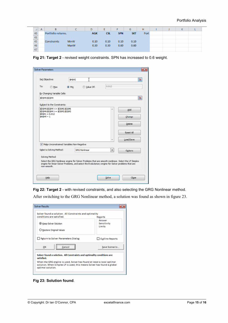
After some experimentation, the set of constraints in Target 2 is evaluated. Target 2: In this scenario, the maximum weight for SPN is increased to 60%, and the target return is set to 1.2% per month. See figure 21, for the weights range, and figure 22 for the revised Solver Parameter set.

Portfolio Analysis


Fig 21: Target 2 - revised weight constraints. SPN has increased to 0.6 weight.

Fig 22: Target 2 - with revised constraints, and also selecting the GRG Nonlinear method.

After switching to the GRG Nonlinear method, a solution was found as shown in figure 23.

Fig 23: Solution found.

Portfolio Analysis


Fig 24: The solution weight

8. Portfolio variance with VBA

In this section, is the VBA code for the function PortSD to estimate the portfolio standard deviation.

VBA: PortSD (Available in the XLFProject.XLF_Module)

10 20 30 40

Function PortSD(Weights As Range, VCV As Range) As Double Dim PortVar As Variant With Application.WorksheetFunction PortVar = .MMult(Weights, .MMult(VCV, .Transpose(Weights))) PortSD = Sqr(.Sum(PortVar)) End With End Function

The weights range is a row vector. The function uses the Excel functions MMULT, TRANSPOSE, and

SUM. In row 30, is the VBA square root function, SQR . The procedure has two important aspects. In line 20, the portfolio variance is calculated. The return

value from the formula is a 1 x 1 array, thus PortVar is of the type Variant. VBA cannot take the square root of a 1 x 1 array, so in line 30, we take the sum of the array, to return a non-array number, then take the square root.

Resources

• The Excel file for this is available at: http://excelatfinance.com/xlf/xlf-portfolio-analysis-v2.xlsm

• An online version of section 1 Descriptive Statistics, and section 2 covariance is available at: http://excelatfinance.com/online/topic/portfolio-analysis-excel/

Portfolio Analysis Published: 21 May 2012 Revised (ver 2): 17 October 2015 Author: Ian O’Connor :: [email protected]

Portfolio analysis - Excel and VBAexcelatfinance.com/xlf/xlf-portfolio-v2.pdf · Covariance with...

Documents

Transcript of Portfolio analysis - Excel and VBAexcelatfinance.com/xlf/xlf-portfolio-v2.pdf · Covariance with...