POLYA’S ENUMERATION THEOREM AND ITS APPLICATIONS …

POLYA’S ENUMERATION THEOREM

AND ITS APPLICATIONS

Master’s ThesisDecember 2015

Author: Matias von BellPrimary Supervisor: Anne-Maria Ernvall-Hytonen

Secondary Supervisor: Erik Elfving

DEPARTMENT OF MATHEMATICS AND STATISTICSUNIVERSITY OF HELSINKI

Faculty of Science Mathematics and Statistics

Matias von Bell

Pólya’s Enumeration Theorem

Mathematics

Pro gradu, Master’s Thesis December 2015 41

Pólya’s Enumeration Theorem, Pólya Theory, Enumeration, Symmetry.

Kumpula Science Library

This thesis presents and proves Pólya’s enumeration theorem (PET) along with the necessarybackground knowledge. Also, applications are presented in coloring problems, graph theory, num-ber theory and chemistry. The statement and proof of PET is preceded by detailed discussions onBurnside’s lemma, the cycle index, weight functions, configurations and the configuration genera-ting function. After the proof of PET, it is applied to the enumerations of colorings of polytopesof dimension 2 and 3, including necklaces, the cube, and the truncated icosahedron. The generalformulas for the number of n-colorings of the latter two are also derived. In number theory, workby Chong-Yun Chao is presented, which uses PET to derive generalized versions of Fermat’s Litt-le Theorem and Gauss’ Theorem. In graph theory, some classic graphical enumeration results ofPólya, Harary and Palmer are presented, particularly the enumeration of the isomorphism classesof unlabeled trees and (v,e)-graphs. The enumeration of all (5,e)-graphs is given as an example.The thesis is concluded with a presentation of how Pólya applied his enumeration technique to theenumeration of chemical compounds.

Tiedekunta/Osasto — Fakultet/Sektion — Faculty Laitos — Institution — Department

Tekijä — Författare — Author

Työn nimi — Arbetets titel — Title

Oppiaine — Läroämne — Subject

Työn laji — Arbetets art — Level Aika — Datum — Month and year Sivumäärä — Sidoantal — Number of pages

Tiivistelmä — Referat — Abstract

Avainsanat — Nyckelord — Keywords

Säilytyspaikka — Förvaringsställe — Where deposited

Muita tietoja — Övriga uppgifter — Additional information

HELSINGIN YLIOPISTO — HELSINGFORS UNIVERSITET — UNIVERSITY OF HELSINKI

i

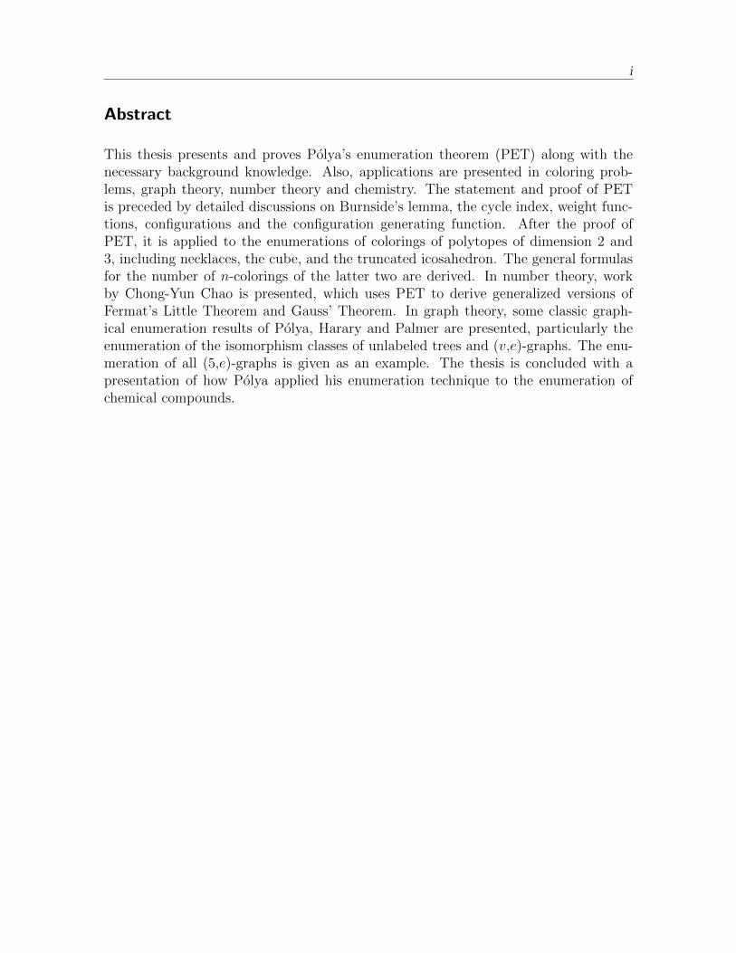
Abstract

This thesis presents and proves Polya’s enumeration theorem (PET) along with thenecessary background knowledge. Also, applications are presented in coloring prob-lems, graph theory, number theory and chemistry. The statement and proof of PETis preceded by detailed discussions on Burnside’s lemma, the cycle index, weight func-tions, configurations and the configuration generating function. After the proof ofPET, it is applied to the enumerations of colorings of polytopes of dimension 2 and3, including necklaces, the cube, and the truncated icosahedron. The general formulasfor the number of n-colorings of the latter two are derived. In number theory, workby Chong-Yun Chao is presented, which uses PET to derive generalized versions ofFermat’s Little Theorem and Gauss’ Theorem. In graph theory, some classic graph-ical enumeration results of Polya, Harary and Palmer are presented, particularly theenumeration of the isomorphism classes of unlabeled trees and (v,e)-graphs. The enu-meration of all (5,e)-graphs is given as an example. The thesis is concluded with apresentation of how Polya applied his enumeration technique to the enumeration ofchemical compounds.

ii

Acknowledgements

I would like to say a big thanks to my primary supervisor Anne-Maria Ernvall-Hytonenfor her guidance, extremely helpful comments and suggestions. Also to Erik Elfving forhis valuable feedback, assistance in my finding an interesting topic and recommendinga great primary supervisor. My thanks also go to the University of Helsinki for a greatstudying experience. I would like to thank all of my teachers and professors throughoutmy mathematical career so far. Particularly Kenneth Rietz, who not only showed methe beauty in mathematics, but also became a mentor and friend. I would also like saythank you to all the patient listeners who have made the mistake of inquiring aboutmy thesis topic. An enormous thanks goes to my parents for their love and support,and to Evie, my wife-to-be and love of my life. Above all IXΘΥΣ.

Contents

Abstract . . . . . . . . . . . . . . . . . . . . . . . . . . . . . . . . . . . . . . i

Acknowledgements . . . . . . . . . . . . . . . . . . . . . . . . . . . . . . . . ii

1. Introduction . . . . . . . . . . . . . . . . . . . . . . . . . . . . . . . . . . . . 1

2. Preliminary Concepts . . . . . . . . . . . . . . . . . . . . . . . . . . . . . . . 3

2.1 Group Theory . . . . . . . . . . . . . . . . . . . . . . . . . . . . . . . . 3

2.2 Equivalence Relations . . . . . . . . . . . . . . . . . . . . . . . . . . . . 7

2.3 Generating Functions . . . . . . . . . . . . . . . . . . . . . . . . . . . . 8

3. Burnside’s Lemma . . . . . . . . . . . . . . . . . . . . . . . . . . . . . . . . 9

3.1 Burnside’s Lemma . . . . . . . . . . . . . . . . . . . . . . . . . . . . . 9

3.2 Coloring the Cube . . . . . . . . . . . . . . . . . . . . . . . . . . . . . 10

4. The Cycle Index . . . . . . . . . . . . . . . . . . . . . . . . . . . . . . . . . 13

4.1 The Cycle Index . . . . . . . . . . . . . . . . . . . . . . . . . . . . . . 13

4.2 Special Cases . . . . . . . . . . . . . . . . . . . . . . . . . . . . . . . . 15

5. Polya’s Enumeration Theorem . . . . . . . . . . . . . . . . . . . . . . . . . . 17

5.1 Configurations and Weights . . . . . . . . . . . . . . . . . . . . . . . . 17

5.2 The Configuration Generating Function . . . . . . . . . . . . . . . . . . 21

5.3 Polya’s Enumeration Theorem . . . . . . . . . . . . . . . . . . . . . . . 22

6. Applications . . . . . . . . . . . . . . . . . . . . . . . . . . . . . . . . . . . . 24

6.1 Coloring Polytopes in Dimensions 2 and 3 . . . . . . . . . . . . . . . . 24

6.1.1 Necklaces . . . . . . . . . . . . . . . . . . . . . . . . . . . . . . 24

6.1.2 The Cube . . . . . . . . . . . . . . . . . . . . . . . . . . . . . . 26

Contents iv

6.1.3 The Truncated Icosahedron . . . . . . . . . . . . . . . . . . . . 27

6.2 Number Theory . . . . . . . . . . . . . . . . . . . . . . . . . . . . . . . 29

6.3 Graph Theory . . . . . . . . . . . . . . . . . . . . . . . . . . . . . . . . 31

6.3.1 Isomorphism Classes of Rooted Trees . . . . . . . . . . . . . . . 31

6.3.2 Isomorphism Classes of (v,e) Graphs . . . . . . . . . . . . . . . 33

6.4 Enumeration of Chemical Compounds . . . . . . . . . . . . . . . . . . 36

7. Conclusion . . . . . . . . . . . . . . . . . . . . . . . . . . . . . . . . . . . . . 40

Bibliography . . . . . . . . . . . . . . . . . . . . . . . . . . . . . . . . . . . . . 41

1. Introduction 1

1 Introduction

The number of colorings of the six faces of a cube fixed in space using n colors iseasily found to be n6. Some of the colorings, however, are indistinguishable from oneanother if one allows the cube to be rotated in space. Enumerating the possible distinctn-colorings, taking rotations into consideration, becomes a non-trivial problem. It’ssolution can be found using group theory, particularly as an application of Burnside’slemma. Supposing further, that we wish to find the number of distinct colorings underrotations such that two faces have color A and four faces have color B, then Burnside’slemma alone is no longer sufficient. However, building on Burnside’s lemma, Polya’sEnumeration Theorem (hereafter PET) proved to answer not only this question, buta whole class of related problems, which previously only had ad hoc solutions.[7]

In 1937, Hungarian mathematician George Polya published a groundbreaking pa-per in combinatorial analysis describing a theorem which allowed a whole new classof enumeration problems to be solved. Entitled Kombinatorische Anzahlbestimmungenfur Gruppen, Graphen und chemische Verbindungen, the paper ran over 100 pages, de-scribing in depth PET and its applications in enumerating groups, graphs and chemicalcompounds. These applications brought Polya’s enumeration technique to the atten-tion of the wider mathematical community, and many more applications have sincebeen found. In 1960, it was discovered that an equivalent theorem to PET had beenpublished by J. H. Redfield ten years before Polya in 1927. Thus PET is sometimesknown as the Polya-Redfield Theorem.[7]

PET can be presented and explained using many different approaches.[7] In thisthesis we follow mainly the approach of De Bruijn in [2] and Harary [4], as the generalityof the theorem surfaces clearly. In its general form PET enumerates distinct functionsbetween two non-empty sets X and Y , where X has a group of permutations G actingon its elements. The “colorings” then become equivalence classes induced in a naturalway by G in Y X , which are known as configurations. Each permutation group hasassociated with it what Polya called the cycle index, which is a polynomial that isconstructed based on the cycle structure of the group. PET then uses the cycle indexassociated with the group and produces a generating function which enumerates allpossible configurations. Taking the cube coloring problem above, we have the group ofrotational symmetries acting on the faces of the cube and the set of colors {A,B}. Usingthe appropriate cycle index, PET produces a generating function where the coefficient

1. Introduction 2

of each AiBj-term gives the number colorings with i faces of color A and j faces ofcolor B. In this manner PET simultaneously enumerates all possible n-colorings.

After reviewing the required background knowledge, primarily in group theory, westate and prove Burnside’s lemma. It is then applied to the cube coloring problem,which serves as a useful explanatory example throughout the thesis. Then, followingdiscussions on the cycle index we proceed to explain and prove PET in detail. Thethesis is concluded with several applications of PET. First it is applied to variouscoloring problems for necklaces and polyhedra. Further applications are given in thefields of number theory, graph theory, and chemistry. A general understanding of thesetopics is assumed.

2. Preliminary Concepts 3

2 Preliminary Concepts

Although in its essence PET is a combinatorial result, much of the machinery under-lying it is algebraic in nature. This is evident from the fact that PET is based onBurnside’s lemma, which is an important group theoretical result. Therefore, the fo-cus of this chapter is on the underlying group theory. The basic ideas of equivalencerelations and generating functions are also required in understanding PET, so they arebriefly reviewed as well.

2.1 Group Theory

We begin by defining and reviewing some group theoretical concepts. In this sectionsome results are stated without proof, as the proofs can be found in most standardbooks on algebra.

Definition 2.1. A group, denoted by (G, ∗), is a non-empty set G equipped with abinary operation ∗ such that the following properties hold:

(i) (Closure). If elements a and b are in G, then a ∗ b ∈ G.

(ii) (Associativity). If a,b, and c are elements in G, then a ∗ (b ∗ c) = (a ∗ b) ∗ c.

(iii) (Identity element). There exists an element e ∈ G such that e ∗ a = a = a ∗ e forall a ∈ G. The element e is known as the identity element.

(iv) (Inverse elements). If a ∈ G, then there exists an element a−1 ∈ G such thata ∗ a−1 = e = a−1 ∗ a. The element a−1 is known as the inverse element of a.

The group (G, ∗) is said to be abelian or commutative, if it also satisfies

(v) (Commutativity). For all a and b in G, a ∗ b = b ∗ a.

The order of the group (G, ∗) is is the cardinality of the set G and it is denoted by|(G, ∗)|.


From this point on, if the group operation is clear from the context, the multiplica-tive notation will be used. In other words a ∗ b will simply be denoted by ab.

Definition 2.2. If G is a group, then any subset H of G which is also a group underthe same operation as G is known as a subgroup of G. If H is a subgroup of G, onetypically writes H ≤ G.

Definition 2.3. If G is a group, H ≤ G, and g ∈ G, then the left coset of H withrespect to g is the set gH = {gh |h ∈ H}. The set of all left cosets of H in G is denotedby G/H. The number of left cosets of H in G is denoted by [G : H] and is known asthe index of H.

Theorem 2.4. (Lagrange’s theorem) Let G be a group. If H ≤ G, then

|G| = [G : H] · |H|.

Definition 2.5. Let A be a set, and f : A → A a bijective function. The function fis known as a permutation of A. If SA = {f : A → A | f is a permutation of A},and ◦ represents the composition of functions, then (SA, ◦) forms a group known as thesymmetric group of A. A subgroup of (SA, ◦) is known as a group of permuta-tions. If A = {1, 2, ..., n}, the symmetric group of A is denoted by Sn.

It is standard to represent a permutation σ ∈ Sn in one of two ways. The firstnotation is to list the elements 1, 2, ..., n in parentheses with their image under thepermutation σ beneath them as follows1:

σ =

(1 2 · · · n

σ(1) σ(2) · · · σ(n)

)The second standard notation for a permutation is known as cycle notation. It is

more compact and will thus be used. A k-cycle is a sequence (j1j2...jk) of elementsfrom {1, 2, ..., n} that denotes the permutation for which σ(j1) = j2, σ(j2) = j3, ...,σ(jk−1) = jk, σ(jk) = j1.

Example 2.6. Consider the permutation σ in the symmetric group S4 such that σ(1) =4, σ(2) = 1, σ(3) = 3, and σ(4) = 2.

In Cauchy notation:

σ =

(1 2 3 44 1 3 2

)In cycle notation:

σ = (142)(3) = (142)

1 This notation is attributed to Augustin-Louis Cauchy [10]


1-cycles are often left out, but sometimes showing them is useful2. Also, the startingelement may vary, so the cycles (142) and (421) are equivalent.

Theorem 2.7. Let σ ∈ Sn. There exists a unique product of disjoint k-cycles τ1, τ2,..., τm (including 1-cycles) such that σ = τ1τ2...τm.

The product in Theorem 2.7 is unique up to the order of the k-cycles, and is knownas the complete factorization of the permutation σ.

Definition 2.8. Let G be a group and let X be a set. A map γ : G×X → X definedby γ(g, x) = gx is said to be a left group action if the following conditions hold:

(i) ex = x, when e is the identity element of G.

(ii) (gh)(x) = g(h(x)) for all g,h ∈ G.

One says that G acts on X. When G is a permutation group, the action that sends(g, x) → gx is known as the natural action. It will be assumed unless otherwisestated.

Definition 2.9. Let the group G act on the set X. If x ∈ X, then the orbit of x isthe set

Gx = {gx | g ∈ G}.

Let A ⊂ X. The stabilizer of A is the subgroup of G defined by

GA = {g ∈ G | ga ∈ Afor all a ∈ A}.

If A = {x} is a singleton set, then the stabilizer of {x} is Gx = {g ∈ G | gx = x}. Whena group G acts on a set X, a permutation g ∈ G may keep an element x ∈ X fixed, i.e.gx = x. The set of all such fixed points of g is denoted by Fix(g) = {x ∈ X | gx = x}

Lemma 2.10. If the group G acts on the non-empty set X, then the set of all orbits,denoted by X/G, forms a partition of X.

Proof. Let A ∈ X/G. The orbit A is clearly non-empty since A = Gx for some x ∈ Xand Gx 6= ∅ for all x ∈ X. Since ex = x for all x ∈ X, each x belongs to some orbit inX/G. Hence ∪A∈X/GA = X. Now it remains to be shown that the union of any twoorbits are disjoint. Suppose not, then there exists x ∈ X such that x ∈ A and x ∈ Bbut A 6= B. Since A = Gy and B = Gz for some y, z ∈ X, we have x = gy and x = g′zfor some g, g′ ∈ G. Now since A 6= B, and we can assume WLOG A ) B, i.e. thereexists a ∈ Gy such that a /∈ Gz. Because a = hy for some h ∈ G and x = gy, we haveh−1a = g−1x. It follows that a = hg−1x = hg−1g′z ∈ Gz, which is a contradiction.Therefore the union of any two orbits is disjoint. Thus all conditions of a partition aresatisfied.

2 For example in section 4.1.


Example 2.11. Here are some examples.

1 Let G = (Q \ 0, ·), and X = R. Now G acts on R as regular (left) multiplication.The orbits of each x ∈ R is the set Gx = {qx | q ∈ Q} and the stabilizer of eachx is the multiplicative identity 1. The stabilizer of the set A = { π

2n|n ∈ Z} ⊆ R

is the subgroup GA = { 12n|n ∈ Z} ≤ G.

2 Let G = {e, (135)(246), (531)(642), (15)(24), (26)(35), (46)(13)} ≤ S6 and X theset of corners of the hexagon {1, 2, 3, 4, 5, 6}. Now G acts on X by permut-ing the corners. The orbit G3 = {1, 3, 5}, the stabilizer G3 = e and X/G ={{1, 3, 5}, {2, 4, 6}}.

Theorem 2.12. (The Orbit-stabilizer theorem) If the group G acts on a set X andx ∈ X, then there exists a bijection f : G/Gx → Gx such that f(gGx) = gx.

Proof. First we show that the function f : G/Gx → Gx, is well defined when f(gGx) =gx. Let g and g′ belong to the same coset in G/Gx. Now g = g′h for some h ∈ Gx.Since h ∈ Gx it holds that gx = (g′h)x = g′(hx) = g′x. Now we show that f isinjective. Let g′x = gx. Now g−1g′x = x, so g−1g′ ∈ Gx, which implies g′ ∈ gGx. Sincealso g ∈ gGx, we have g and g′ belonging to the same coset, and thus f is injective.Since f is clearly surjective, the proof is complete.

It has been shown that the number of left cosets of Gx is equal to the numberelements in the orbit Gx, i.e. [G : Gx] = |Gx|. Thus, together with Lagrange’stheorem (2.4), the orbit-stabilizer theorem states that |G| = |Gx||Gx|.

Definition 2.13. The cyclic group Cn is the group of rotational symmetries of theregular n-gon. The dihedral group Dn is the group of rotational and reflective sym-metries of a regular n-gon. The alternating group An is a subgroup of Sn with indexequal to 2.

An n-gon has n symmetric rotations and n symmetric reflections, hence the orderof Cn is n and Dn is 2n. Since |Sn| = n!, we have |An| = n!

2.

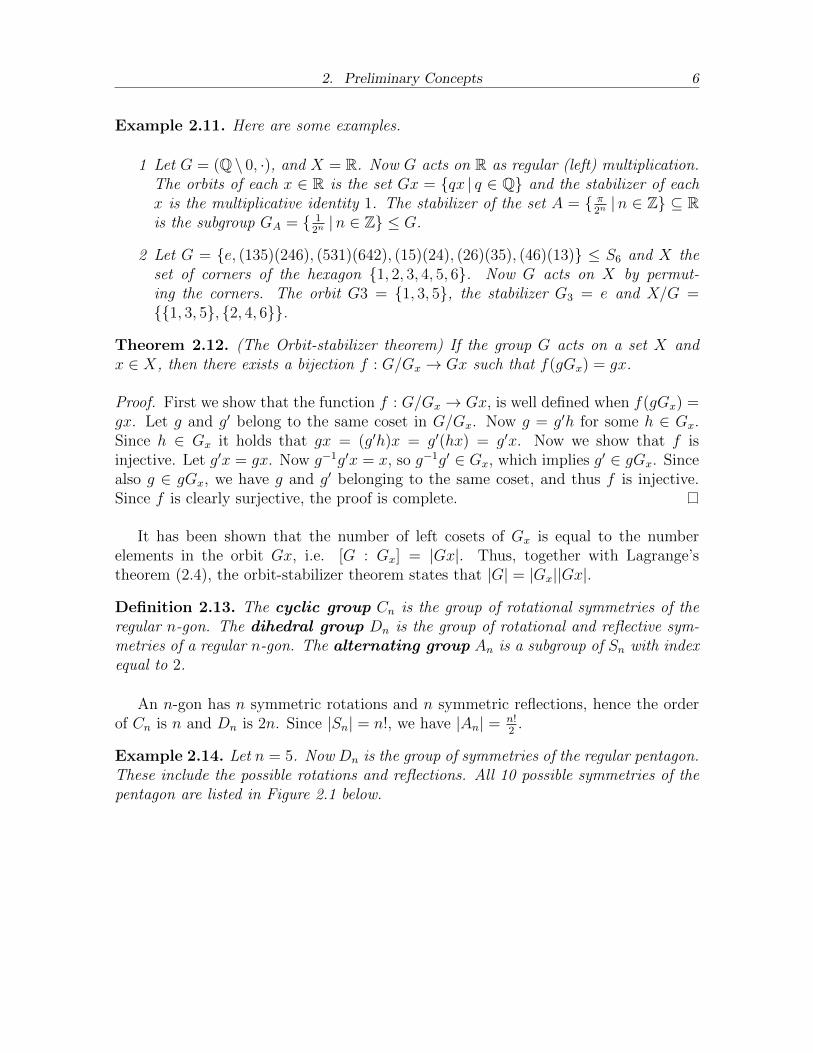
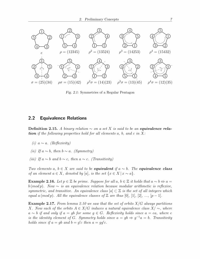
Example 2.14. Let n = 5. Now Dn is the group of symmetries of the regular pentagon.These include the possible rotations and reflections. All 10 possible symmetries of thepentagon are listed in Figure 2.1 below.


2

1

5

4 3

e

3

2

1

5 4

ρ = (12345)

4

3

2

1 5

ρ2 = (13524)

5

4

3

2 1

ρ3 = (14253)

1

5

4

3 2

ρ4 = (15432)

5

1

2

3 4

σ = (25)(34)

4

5

1

2 3

ρσ = (15)(42)

3

4

5

1 2

ρ2σ = (14)(23)

2

3

4

5 1

ρ3σ = (13)(45)

1

2

3

4 5

ρ4σ = (12)(35)

Fig. 2.1: Symmetries of a Regular Pentagon

2.2 Equivalence Relations

Definition 2.15. A binary relation ∼ on a set X is said to be an equivalence rela-tion if the following properties hold for all elements a, b, and c in X:

(i) a ∼ a. (Reflexivity)

(ii) If a ∼ b, then b ∼ a. (Symmetry)

(iii) If a ∼ b and b ∼ c, then a ∼ c. (Transitivity)

Two elements a, b ∈ X are said to be equivalent if a ∼ b. The equivalence classof an element a ∈ X, denoted by [a], is the set {x ∈ X |x ∼ a}.

Example 2.16. Let p ∈ Z be prime. Suppose for all a, b ∈ Z it holds that a ∼ b⇔ a =b (mod p). Now ∼ is an equivalence relation because modular arithmetic is reflexive,symmetric, and transitive. An equivalence class [a] ⊂ Z is the set of all integers whichequal a (mod p). All the equivalence classes of Z are thus [0], [1], [2], ..., [p− 1].

Example 2.17. From lemma 2.10 we saw that the set of orbits X/G always partitionsX. Now each of the orbits A ∈ X/G induces a natural equivalence class X/ ∼, wherea ∼ b if and only if a = gb for some g ∈ G. Reflexivity holds since a = ea, where eis the identity element of G. Symmetry holds since a = gb ⇒ g−1a = b. Transitivityholds since if a = gb and b = g′c then a = gg′c.


Example 2.18. Suppose X and Y are finite sets, G is a group acting on the set X.An equivalence relation ∼ on Y X , the set of all functions from X to Y , can be definedas follows:

f1 ∼ f2 ⇐⇒ ∃ g ∈ G such that f1(gx) = f2(x) for allx ∈ X.

The verification that ∼ is an equivalence relation is straightforward. Choosing g ∈ Gto be the identity permutation we have f1(g(x)) = f1(x) for all x ∈ X, thus f1 ∼ f1 andreflexivity holds. If f1 ∼ f2, then f1(g(x)) = f2(x) for all x ∈ X. Now since g−1 ∈ Gand f1(x) = f1(g

−1g(x)) = f2(g−1(x)) for all x ∈ X, we have f2 ∼ f1. Thus symmetry

holds. If f1 ∼ f2 and f2 ∼ f3, then ∃ g1, g2 ∈ G such that f1(g1(x)) = f2(x) andf2(g2(x)) = f3(x) for all x ∈ X. Now since g1g2 ∈ G and f1(g1g2(x)) = f2(g2(x)) =f3(x), we have f1 ∼ f3. Thus transitivity holds and hence ∼ is an equivalence relation.

2.3 Generating Functions

The theory of generating functions in itself has rich applications to the theory of count-ing [9]. However, here only the basic idea is reviewed, as deeper parts of the theoryare not needed to understand PET.

Definition 2.19. Let a0, a1, a2, a3, ... be a sequence of integers. The formal powerseries

G(an;x) =∞∑n=o

akxn = a0 + a1x+ a2x

2 + a3x3 + · · ·

is called the generating function associated with the sequence a0, a1, a2, a3.... Agenerating function may have more than one variable, in which case it is known as amultivariate generating function and is of the form:

G(a(n1,n2,...,nk);x1, x2, ..., xk) =∞∑

n1,n2,...,nk=o

an1,n2,...,nkxn11 x

n22 · · ·x

nkk

Example 2.20. The following are some basic examples.

1. The generating function of the triangular numbers 1,3,6,10,... is the power series

1 + 3x+ 6x2 + 10x3 + · · · =∞∑n=0

(n+ 2

2

)xn =

1

(1− x)3

2. The multivariate generating function for the binomial coefficients is

G(

(n

k

);x, y) =

∞∑n=0

(nk

)xkyn =

1

1− y − xy

3. Burnside’s Lemma 9

3 Burnside’s Lemma

PET relies heavily on a result from group theory which is often known as Burnside’slemma. Therefore, discussing it is necessary before tackling PET. Burnside’s lemmagets its name after William Burnside, although it was known to Frobenius and in itsessence to Cauchy. It is thus sometimes also called the Cauchy-Frobenius Lemma.[7]Another name for Burnside’s lemma, which sheds more light on its function, is theorbit-counting theorem.

3.1 Burnside’s Lemma

Theorem 3.1. (Burnside’s Lemma) Let a finite group G act on the set X. Thetotal number of orbits, denoted by |X/G|, is given by

|X/G| = 1

|G|∑g∈G

|Fix(g)|.

Burnside’s lemma essentially states that the number of orbits is equal to the averagenumber of elements in X which are fixed by each g ∈ G.

Proof. First we notice that g ∈ Gx if and only if x ∈ Fix(g). Thus we have∑x∈X

|Gx| = |{(g, x) ∈ G×X | gx = x}| =∑g∈G

|Fix(g)| (3.1)

From the orbit-stabilizer theorem 2.12 we have that [G : Gx] = |Gx|, and together withLagrange’s theorem, |G|/|Gx| = |Gx|. Thus |G|/|Gx| = |Gx|, which substituted intothe equation 3.1 above gives

∑x∈X

|G||Gx|

= |G|∑x∈X

1

|Gx|=∑g∈G

|Fix(g)| (3.2)

By Lemma 2.10 we know that the set of orbits partitions the set X. Thus unions oforbits are disjoint and we can write


∑x∈X

1

|Gx|=∑

A∈X/G

∑x∈A

1

|A|=∑

A∈X/G

1 = |X/G| (3.3)

Combining equations 3.2 and 3.3 gives

|X/G| = 1

|G|∑g∈G

|Fix(g)|

3.2 Coloring the Cube

To demonstrate Burnside’s lemma for counting colorings of an object with symmetries,we take a look at the following example.

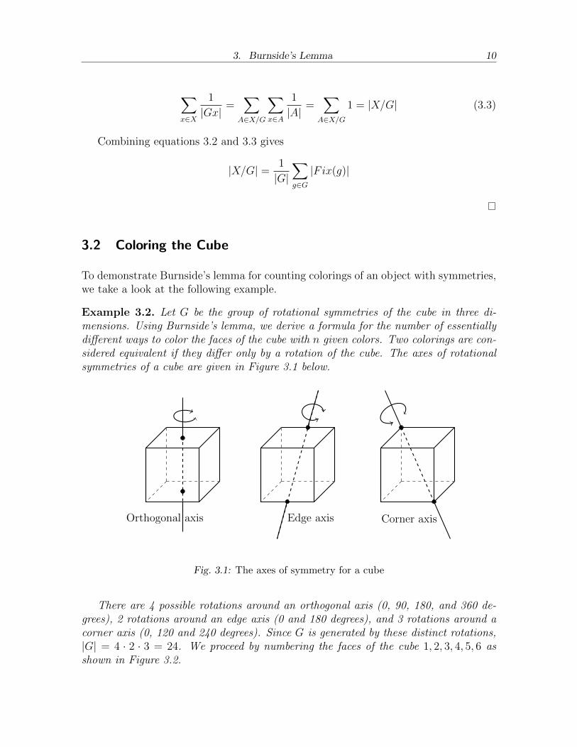
Example 3.2. Let G be the group of rotational symmetries of the cube in three di-mensions. Using Burnside’s lemma, we derive a formula for the number of essentiallydifferent ways to color the faces of the cube with n given colors. Two colorings are con-sidered equivalent if they differ only by a rotation of the cube. The axes of rotationalsymmetries of a cube are given in Figure 3.1 below.

Orthogonal axis Edge axis Corner axis

Fig. 3.1: The axes of symmetry for a cube

There are 4 possible rotations around an orthogonal axis (0, 90, 180, and 360 de-grees), 2 rotations around an edge axis (0 and 180 degrees), and 3 rotations around acorner axis (0, 120 and 240 degrees). Since G is generated by these distinct rotations,|G| = 4 · 2 · 3 = 24. We proceed by numbering the faces of the cube 1, 2, 3, 4, 5, 6 asshown in Figure 3.2.


1

2

3

4

56

Fig. 3.2: Numbering of the cube’s faces

Since colorings are equivalent if they differ only by a rotation, they are equivalentif they belong to the same orbit of G when G acts on the set of faces of the cube.Thus finding distinct colorings reduces to finding the number of orbits of G, and henceBurnside’s lemma can be applied. We need to first find the number of fixed points foreach g ∈ G. If g is the identity rotation, the number of different coloring of the cube issimply n6. If g = (1)(6)(2345), it is a 90◦ rotation around the orthogonal axis. Sinceg holds faces 1 and 6 fixed, and each can be colored with n colors, there are n2 distinctcolorings for them. The remaining faces 2, 3, 4, and 5 are not fixed, but they are in thesame cycle, so they must all be the same color to be invariant under g. Thus they canbe colored in n possible ways. The total number of colorings under g is now n2n = n3.In a similar manner the number of fixed colorings of all 24 permutations in G can befound. One may notice that the number of fixed colorings is the number of cycles ing, including the unit cycles. This is no coincidence, and will be discussed in detail insection 4.1. Table 3.1 shows all 24 permutations in G and the number of coloringswhich they keep fixed.

Axis and degrees of rotation Face permutations g ∈ G |Fix(g)|Identity rotation (1)(2)(3)(4)(5)(6) n6

Orthogonal (90◦ and 270◦)(1)(6)(2345) (2)(4)(1563)(3)(5)(1264) (1)(6)(5432)(2)(4)(3651) (3)(5)(4621)

n3

Orthogonal (180◦)(1)(6)(24)(35)(2)(4)(16)(35)(3)(5)(24)(16)

n4

Edge (180◦)(14)(26)(35) (12)(46)(35)(16)(45)(23) (16)(34)(25)(24)(13)(56) (24)(15)(36)

n3

Corner (120◦ and 240◦)

(154)(263) (123)(456)(152)(346) (143)(256)(451)(362) (321)(654)(251)(643) (341)(652)

n2

Tab. 3.1: The number of fixed n-colorings for each permutation ofthe cube’s faces.


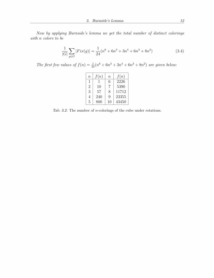
Now by applying Burnside’s lemma we get the total number of distinct coloringswith n colors to be

1

|G|∑g∈G

|Fix(g)| = 1

24(n6 + 6n3 + 3n4 + 6n3 + 8n2) (3.4)

The first few values of f(n) = 124

(n6 + 6n3 + 3n4 + 6n3 + 8n2) are given below:

n f(n) n f(n)1 1 6 22262 10 7 53903 57 8 117124 240 9 233555 800 10 43450

Tab. 3.2: The number of n-colorings of the cube under rotations.

4. The Cycle Index 13

4 The Cycle Index

We saw in chapter 3 the power of Burnside’s lemma in its ability to take into accountsymmetries in counting. Using it, a formula for the n-colorings of the faces of a cubewas found. Suppose, however, that we wish to find a formula for the n-colorings ofthe 32 sides of a truncated icosahedron. The problem could be solved by Burnside’slemma in exactly the same fashion as was done with the cube, but it would be extremelytedious, and therefore we seek a shortcut. This is where the cycle index comes to therescue.

4.1 The Cycle Index

As mentioned in section 2.1, a permutation σ on a finite set X with n elements canbe represented uniquely in its complete factorization σ = τ1τ2...τm, where m ≤ n.We say that σ is of type {b1, b2, ..., bn} where bi is the number i-cycles in the com-plete factorization τ1τ2...τm. For example, the permutation (1532)(46)(87)(9) is of type{1, 2, 0, 1, 0, 0, 0, 0, 0}.

Definition 4.1. Let G be a group of permutations. The cycle index is the polynomialwith n variables x1,x2,...,xn

ZG(x1, x2, ..., xn) =1

|G|∑g∈G

xb11 xb22 · · ·xbnn

where the product xb11 xb22 · · ·xbnn is formed for each g ∈ G from its type {b1, b2, ..., bn}.1

The cycle index depends on the structure of the group action G on the set X. Thusfor each structure of G and different sizes of X we must find a new cycle index. Forthis reason finding the cycle index must be done in a case by case basis, as is done inthe following examples from [2].

Example 4.2. First we revisit the situation in Example 3.2, where we have that G isthe group of rotational symmetries of the cube, and it acts on the faces of the cube. The

1 Polya used the letter Z to hint at the German for cycle index, which is zyklenzeiger.[7]


identity rotation is written in cyclic form (1)(2)(3)(4)(5)(6), so its type is {6, 0, ..., 0}.Thus it contributes the monomial xb11 x

b22 · · ·xbnn = x61 to the cycle index. The orthogonal

rotation of 180◦ characterized by the permutation (1)(6)(24)(35) is of type {2, 2, 0, ..., 0}so it contributes the monomial x21x

22 to the cycle index. Continuing in this way through

all g ∈ G, we get the cycle index

ZG(x1, x2, x3, x4) =1

24(x61 + 6x21x4 + 3x21x

22 + 6x32 + 8x23). (4.1)

Substituting xi = n for all i in equation 4.1 gives equation 3.4.

Example 4.3. Suppose G is again the group of rotational symmetries of the cube, butthis time it acts on the set of vertices of the cube V , where |V | = 8. We have the samesets of rotational symmetries:

(a) Identity rotation.

(b) Six rotations of the orthogonal axis by 90◦ and 270◦.

(c) Three rotations of the orthogonal axis by 180◦.

(d) Six rotations of the edge axis by 180◦.

(e) Eight rotations of the corner axis by 120◦ and 240◦.

In each case we can visualize the cycles, and directly pick out the cycle types. Theidentity rotation has type {8,0,0,...,0}. The rotations in (b) have type {0,0,0,2,0,...,0}.The rotations in (c) have type {0,4,0,0,...,0}. The rotations in (d) have type {0,4,0,...,0}.The rotations in (e) have type {2,0,2,0,...,0}. Thus the cycle index is

ZG(x1, x2, x3, x4) =1

24(x81 + 6x24 + 3x42 + 6x42 + 8x21x

23).

Similarly, if G acts on the set of edges of the cube E, we can find the cycle index asfollows, noting that |E| = 12. The identity rotation has type {12,0,0,...,0}. The rota-tions in (b) have type {0,0,0,3,0,...,0}. The rotations in (c) have type {0,6,0,0,...,0}.The rotations in (d) have type {2,5,0,...,0}. The rotations in (e) have type {0,0,4,0,...,0}.Thus the cycle index is

ZG(x1, x2, x3, x4) =1

24(x121 + 6x44 + 3x62 + 6x21x

52 + 8x43).


4.2 Special Cases

In his original 1937 paper, Polya lists the cycle indices of some special cases. Inparticular, he gives them for the natural actions of common subgroups of the symmetricgroup.

The Trivial Permutation GroupThe trivial permutation group En ≤ Sn is the permutation group containing only theidentity permutation. The cycle index is

ZEn(x1) = xn1

The Cyclic GroupThe cyclic permutation group Cn ≤ Sn is the permutation group which contains allcyclic permutations of n elements. It can be thought of as the group of rotationalsymmetries of an n-gon. The cycle index is then given by

ZCn(x1, x2, ..., xn) =1

n

∑d|n

φ(d)xn/dd

where φ is the Euler totient function.[7]

Example 4.4. In the case n = 5, C5 is the group of rotational symmetries of thepentagon. The cycle index is then

ZC5(x1, x2, ..., xn) =1

5

∑d|5

φ(d)x5/dd

=1

5

(x51 + 4x5

).

The Dihedral GroupThe dihedral group Dn, as in definition 2.13, includes the rotations and reflections ofthe n-gon. The cycle index now varies depending of whether n is even or odd.[7]

ZDn(x1, x2, ..., xn) =1

2ZCn(x1, x2, ..., xn) +

{12x1x

(n−1)/22 if n is odd

14

(x21x

(n−2)/22 + x

n/22

)if n is even

The Symmetric Group2

Let (j) denote a partition of n, that is, (j) ∈ {(j1, j2, ..., jn) | j1 + 2j2 + ...+ njn = n}.2 In [7] Polya gives only the cycle index for cases n = 1, 2, 3, 4 for the symmetric group and alter-

nating group. The general cases are given by Harary and Palmer in [4].


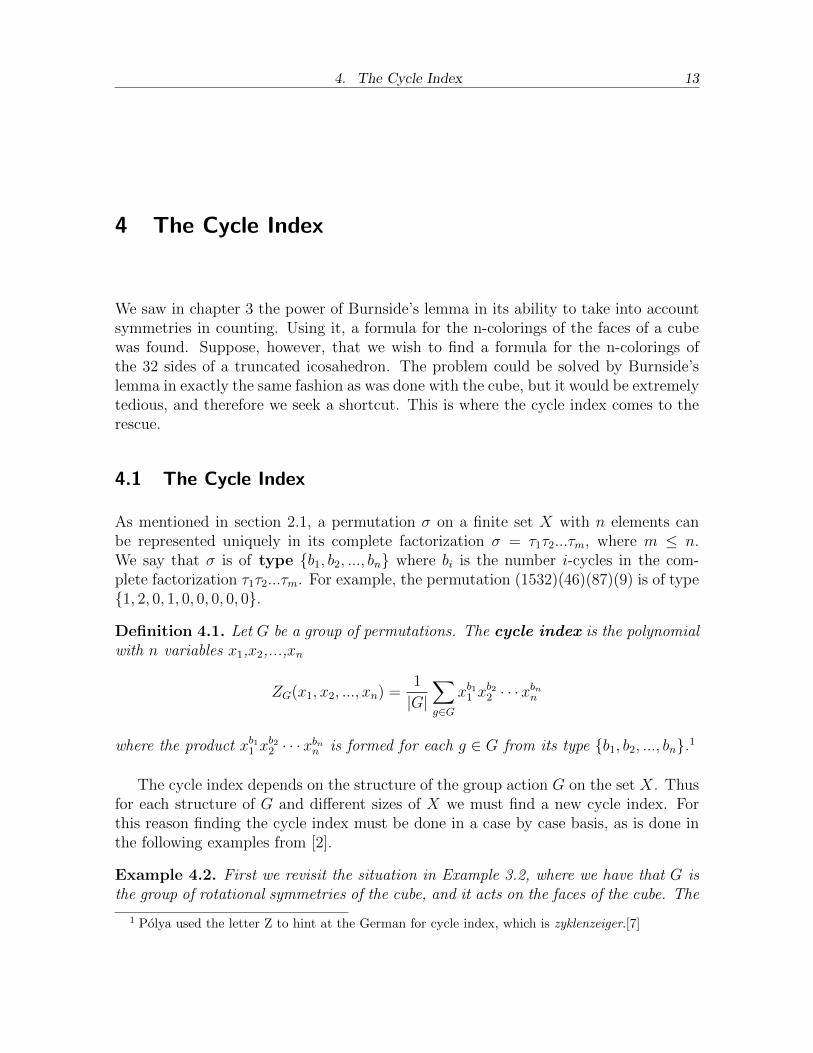
The cycle index of the symmetric group acting on a set of n elements is then given by:

ZSn(x1, x2, ..., xn) =∑(j)

1∏kjkjk!

n∏k=1

xjkk

where the sum is taken over all partitions of n.

The Alternating GroupThe cycle index of the alternating group acting on a set of n elements is given by

ZAn(x1, x2, ..., xn) = ZSn(x1, x2, ..., xn) + ZSn(x1,−x2, x3,−x4, ...,±xn).

5. Polya’s Enumeration Theorem 17

5 Polya’s Enumeration Theorem

5.1 Configurations and Weights

In this section we define the concept of a “configuration” along with its “weight” in thecontext of Polya theory. Throughout the section we will focus on functions betweentwo finite sets, X and Y . The set of all function from X to Y is denoted by Y X , andit is well known that its cardinality is given by |Y ||X|.

Definition 5.1. Let X and Y be finite sets, with the group G acting on the set X. Let∼ be the equivalence relation on Y X given by

f1 ∼ f2 ⇐⇒ ∃ g ∈ G such that f1(gx) = f2(x) for allx ∈ X.1

The equivalence classes of ∼ will be called configurations.2

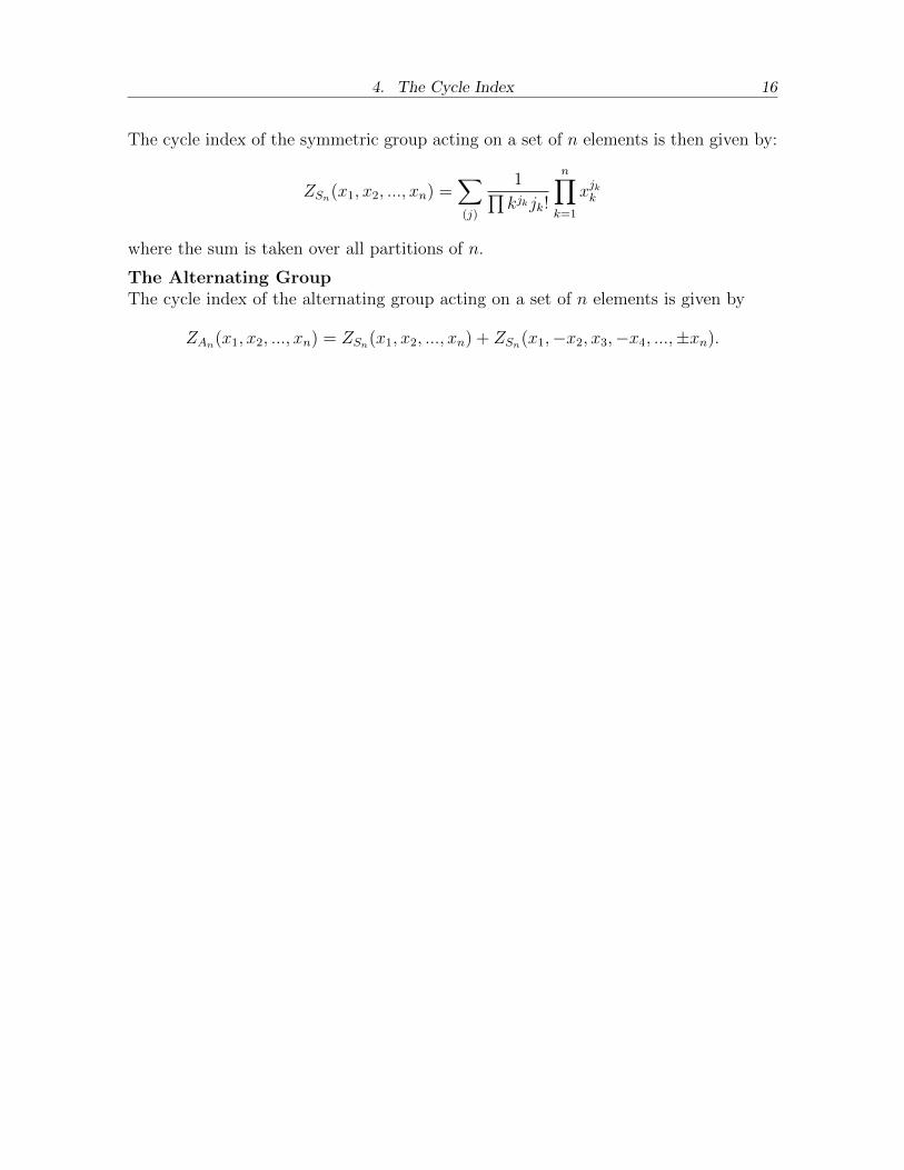
Example 5.2. Let X = {1, 2, 3, 4, 5} be the set of numbered edges of a pentagon, letG be the cyclic group C5, and Y the set containing the words “black” and “white”.

2

1

5

4 3

Fig. 5.1: Pengaton with numbered corners.

There are now eight distinct configurations, as seen in Figure 5.2

1 The verification that ∼ is an equivalence relation was done in example 2.18.2 Some authors, such as De Bruijn and Graver, call these equivalence classes “patterns”.


r

r

r

r r

c1

3

2

5

c2

4

3

5

c3

5

4

2

c4

5

1

c5

5

3

c6

4

c7 c8

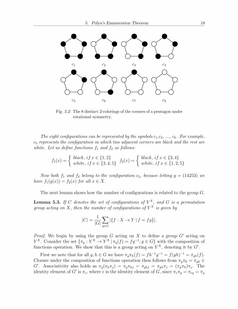
Fig. 5.2: The 8 distinct 2-colorings of the corners of a pentagon underrotational symmetry.

The eight configurations can be represented by the symbols c1,c2, ..., c8. For example,c5 represents the configuration in which two adjacent corners are black and the rest arewhite. Let us define functions f1 and f2 as follows:

f1(x) =

{black, if x ∈ {1, 2}white, if x ∈ {3, 4, 5} f2(x) =

{black, if x ∈ {3, 4}white, if x ∈ {1, 2, 5}

Now both f1 and f2 belong to the configuration c5, because letting g = (14253) wehave f1(g(x)) = f2(x) for all x ∈ X.

The next lemma shows how the number of configurations is related to the group G.

Lemma 5.3. If C denotes the set of configurations of Y X , and G is a permutationgroup acting on X, then the number of configurations of Y X is given by

|C| = 1

|G|∑g∈G

|{f : X → Y | f = fg}|.

Proof. We begin by using the group G acting on X to define a group G′ acting onY X . Consider the set {πg : Y X → Y X |πg(f) = fg−1, g ∈ G} with the composition offunctions operation. We show that this is a group acting on Y X , denoting it by G′.

First we note that for all g, h ∈ G we have πgπh(f) = fh−1g−1 = f(gh)−1 = πgh(f).Closure under the composition of functions operation then follows from πgπh = πgh ∈G′. Associativity also holds as πg(πhπj) = πgπhj = πghj = πghπj = (πgπh)πj. Theidentity element of G′ is πe, where e is the identity element of G, since πeπg = πeg = πg


for all πg ∈ G′. The inverse element of πg is πg−1 since πgπg−1 = πgg−1 = πe. ThusG′ is a group of permutations on Y X and it acts on Y X because πe(f) = fe = f and(πgπh)(f) = πgh(f) = f(gh)−1 = fh−1g−1 = πg(πh(f)). Let O denote an orbit inY X/G′ and let D denote a configuration in C. Now

f1, f2 ∈ O ⇔ f1 = πg(f2) = f2g−1 for some g ∈ G

⇔ f1g = f2 for some g ∈ G⇔ f1, f2 ∈ D.

Hence functions belong to the same orbit of Y X/G′ iff they belong to the same config-uration in C, and therefore

|C| = |Y X/G′|. (5.1)

Applying Burnside’s lemma (theorem 3.1) to the RHS of equation 5.1 gives:

|C| = 1

|G′|∑πg∈G′

|Fix(πg)|. (5.2)

Next we note that since πg(f) = f ⇔ f = fg−1 ⇔ f = fg, we have

Fix(πg) = {f : X → Y | πg(f) = f} = {f : X → Y | f = fg}. (5.3)

Finally substituting Equation 5.3 into Equation 5.2 and noting that πg ∈ G iff g ∈ Ggives the result

|C| = 1

|G|∑g∈G

|{f : X → Y | f = fg}|.

In Example 5.2 the colors were represented by the the words “black” and “white”,and configurations were represented with symbols c1, c2, ..., c8. By introducing the con-cept of weights to the colors and configurations, we can manipulate them algebraically.

Definition 5.4. Let Y be a finite set, let R be a commutative ring which contains therational numbers as a subset3, and let w : Y → R. The weight of each y ∈ Y isthe element w(y). The weight of a function f : X → Y , denoted by W (f), is theproduct:

W (f) =∏x∈X

w(f(x)).

3 For example a polynomial ring Q[X1, ..., Xn]. This construction allows for the multiplication ofweights by rational coefficients in the cycle index.


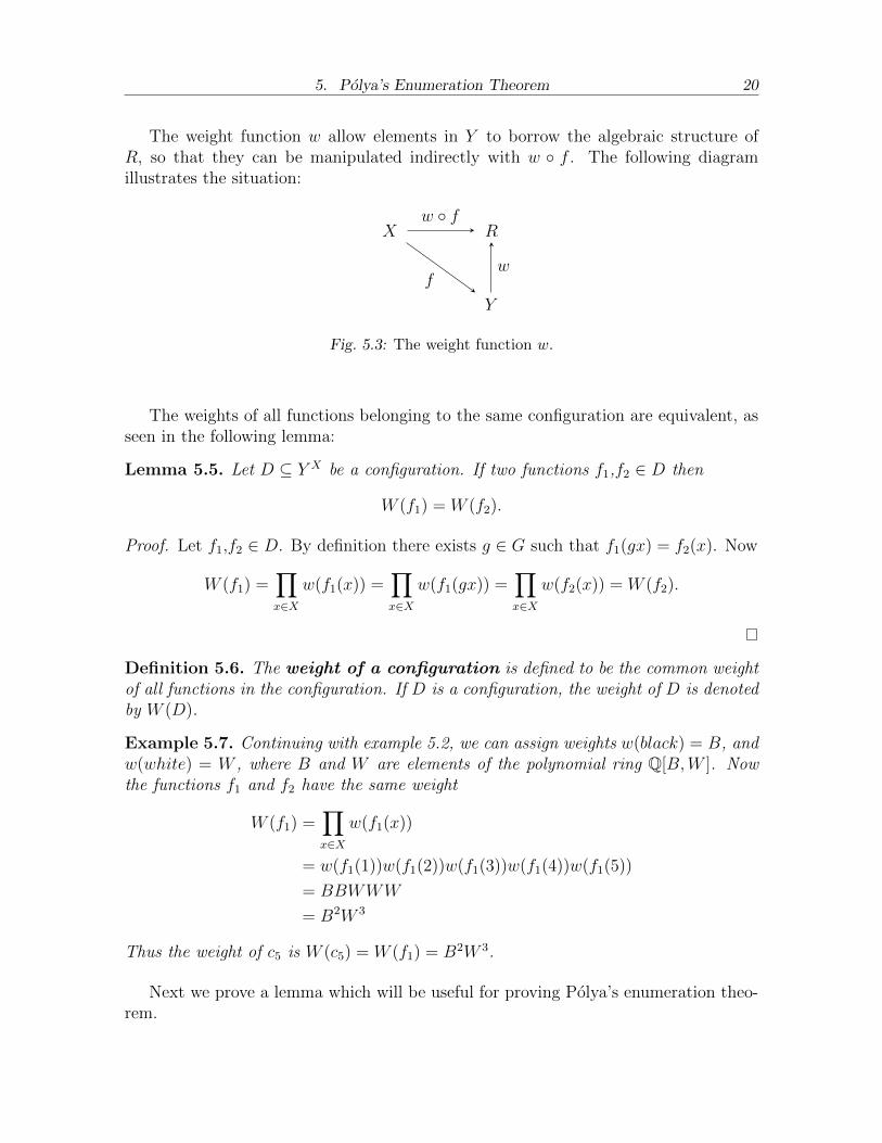
The weight function w allow elements in Y to borrow the algebraic structure ofR, so that they can be manipulated indirectly with w ◦ f . The following diagramillustrates the situation:

X R

Y

w ◦ f

fw

Fig. 5.3: The weight function w.

The weights of all functions belonging to the same configuration are equivalent, asseen in the following lemma:

Lemma 5.5. Let D ⊆ Y X be a configuration. If two functions f1,f2 ∈ D then

W (f1) = W (f2).

Proof. Let f1,f2 ∈ D. By definition there exists g ∈ G such that f1(gx) = f2(x). Now

W (f1) =∏x∈X

w(f1(x)) =∏x∈X

w(f1(gx)) =∏x∈X

w(f2(x)) = W (f2).

Definition 5.6. The weight of a configuration is defined to be the common weightof all functions in the configuration. If D is a configuration, the weight of D is denotedby W (D).

Example 5.7. Continuing with example 5.2, we can assign weights w(black) = B, andw(white) = W , where B and W are elements of the polynomial ring Q[B,W ]. Nowthe functions f1 and f2 have the same weight

W (f1) =∏x∈X

w(f1(x))

= w(f1(1))w(f1(2))w(f1(3))w(f1(4))w(f1(5))

= BBWWW

= B2W 3

Thus the weight of c5 is W (c5) = W (f1) = B2W 3.

Next we prove a lemma which will be useful for proving Polya’s enumeration theo-rem.


Lemma 5.8. Let X be a disjoint union of sets X1, X2,..., Xn. If S ⊂ Y X is the setof functions f which are constant on each Xi, then

∑f∈S

W (f) =n∏i=1

∑y∈Y

w(y)|Xi|

Proof. Suppose Y = {y1, ..., ym}. We begin by expanding the product

k∏i=1

∑y∈Y

w(y)|Xi| =(w(y1)

|X1| + · · ·+ w(ym)|X1|) (w(y1)

|X2| + · · ·+ w(ym)|X2|)· · ·(

w(y1)|Xn| + · · ·+ w(ym)|Xn|

).

(5.4)

Multiplying out the RHS of equation 5.4 gives a sum(w(y1)

|X1|w(y1)|X2| · · ·w(y1)

|Xn|)

+(w(y1)

|X1|w(y1)|X2| · · ·w(y2)

|Xn|)

+

· · ·+(w(ym)|X1|w(ym)|X2| · · ·w(ym)|Xn|

).

(5.5)

Since f is constant in each Xi iff f ∈ S, each term in this sum corresponds to a singlefunction f ∈ S. Thus the sum 5.5 can be written as∑

f∈S

w(f(x1))|X1|w(f(x2))

|X2| · · ·w(f(xn))|Xn| (5.6)

where xi ∈ Xi for each i ∈ {1, ..., n}. Finally we notice that 5.6 can also be written as

∑f∈S

(∏x∈X1

w(f(x))

)(∏x∈X2

w(f(x))

)· · ·

(∏x∈Xn

w(f(x))

)=∑f∈S

∏x∈X

w(f(x))

=∑f∈S

W (f)

Thus the lemma holds.

5.2 The Configuration Generating Function

Given a set of configurations C on Y X , the configuration generating function (orCGF) is defined by

F (C) =∑c∈C

W (c).


Example 5.9. Given the situation in example 5.2, the set of configurations is C ={c1, c2, ..., c8}. Thus the CGF becomes∑

c∈CW (c) = W (c1) +W (c2) + · · ·+W (c8)= B5 +B4W +B3W 2 +B3W 2 +B2W 3 +B2W 3 +BW 4 +W 5

= B5 +B4W + 2B3W 2 + 2B2W 3 +BW 4 +W 5.

The CGF thereby lists all possible weights of configurations with the coefficientrepresenting the number configurations with the given weight. For example, the weightB2W 3 has coefficient 2, so we know that there are two distinct configurations withweight B2W 3. In other words there are two distinct colorings of the corners of thepentagon such that two corners are black and three are white. Thus knowing theCGF, we know how many distinct colorings there are for each set of weights. To findthe total number of colorings, we can simply assign weights w(white) = w(black) = 1which gives W (ci) = 1 for all i. Now the CGF gives F (C) = 8, the number of distinctcolorings.

5.3 Polya’s Enumeration Theorem

Theorem 5.10. (Polya’s Enumeration Theorem) Let X and Y be finite sets,with |X| = n. Let G be a group acting on X and let ZG be the cycle index polynomial.If w is the weight function on Y , then the configuration generating function is givenby:

ZG

(∑y∈Y

w(y),∑y∈Y

w(y)2, ...,∑y∈Y

w(y)n

).

The special case of assigning w(y) = 1 for all y ∈ Y gives the total number of configu-rations: ZG(|Y |, |Y |, ..., |Y |).

Proof. Let Sω ⊆ Y X be the set of functions that have weight ω. Let φω(g) = {f : X →Y | f = fg, W (f) = ω}. By lemma 5.3 the number of configurations in Sω is given by

|Sω| =1

|G|∑g∈G

|φω(g)|. (5.7)

Thus multiplying by ω and summing over all values of ω gives the CGF:∑c∈C

W (c) =∑ω

ω|Sω| =1

|G|∑ω

∑g∈G

ω|φω(g)|. (5.8)

Letting φ(g) denote the set {f : X → Y | f = fg}, we have that∑ω

ω|φω(g)| =∑f∈φ(g)

W (f). (5.9)


Since the double summation in 5.8 is taken over finite sets, the order of the summationmay be switched. Thus switching the order of summation and combining with 5.9 givesthe CGF ∑

c∈C

W (c) =1

|G|∑g∈G

∑f∈φ(g)

W (f). (5.10)

Every g ∈ G permutes the set X. Therefore each g splits X into a disjoint union ofm cycles X1, X2, · · · ,Xm, where m ≤ n. If f ∈ S, then f = fg = fg2 = ..., i.e. f isconstant on each Xi. If f is constant on each Xi, then f = fg, and hence f ∈ S. Nowapplying lemma 5.8 gives

∑f∈φ(g)

W (f) =m∏i=1

∑y∈Y

w(y)|Xi| =

(∑y∈Y

w(y)|X1|

)(∑y∈Y

w(y)|X2|

)· · ·

(∑y∈Y

w(y)|Xm|

).

(5.11)If the cycle type of g is {b1, b2, , ..., bn}, then in |X1|, |X2|,..., |Xm|, the number i occursbi times. Thus we can write 5.11 as

∑f∈φ(g)

W (f) =

(∑y∈Y

w(y)

)b1 (∑y∈Y

w(y)2

)b2

· · ·

(∑y∈Y

w(y)n

)bn

. (5.12)

Substituting equation 5.12 into 5.10 gives the CGF:

1

|G|∑g∈G

(∑y∈Y

w(y)

)b1 (∑y∈Y

w(y)2

)b2

· · ·

(∑y∈Y

w(y)n

)bn . (5.13)

Now we simply notice that 5.13 is precisely the cycle index

ZG

(∑y∈Y

w(y),∑y∈Y

w(y)2, · · · ,∑y∈Y

w(y)n

).

This proves Polya’s Enumeration Theorem.

6. Applications 24

6 Applications

The beauty in PET is its generality, which leads to a diverse set of applications. In his1937 paper Polya gave applications of PET in the enumeration of graphs and chemicalcompounds. Since then, as PET came to the attention of the wider mathematicalcommunity, numerous new applications have been found. Within mathematics, appli-cations apart from graph theory include those in logic, number theory, and the study ofquadratic forms. Applications outside of mathematics are found in physics, chemistry,and even music theory.[7]

This chapter begins by discussing the applications of PET to the coloring of poly-topes of dimension 2 and 3. Then we take a look at how PET can, perhaps unexpect-edly, be used in number theory to produce a neat generalization of Fermat’s theoremand Gauss’ theorem. In the theory of graphical enumeration, the important appli-cations of PET in enumerating trees and (v, e)-graphs is discussed. The chapter isconcluded with some of Polya’s examples in chemical enumeration.

6.1 Coloring Polytopes in Dimensions 2 and 3

In this section some natural applications of PET are given in the coloring of poly-gons and polyhedra. The theory is the same for higher dimensional polytopes, butvisualization becomes difficult. Some examples given in this section are ones whichhave been partially discussed in earlier chapters. Particularly the coloring of the cubeis presented again so that the reader may appreciate the simplicity and generality ofPET in comparison to Burnside’s lemma.

6.1.1 Necklaces

The regular polygons with colored vertices are sometimes called necklaces, and the ver-tices are called beads. PET can be used to enumerate the number of beaded necklaceswith n colors.

Example 6.1. Given a set of black and white beads, how many distinct five beadednecklaces can be made if one allows for rotation of the necklaces? How many of themcontain two black beads and three white beads?

6. Applications 25

We let X be a five beaded necklace, and Y be the set containing the two colors blackand white. The relevant permutation group G is the cyclic group C5. We assign weightsto the two colors as follows: w(black) = B and w(white) = W . Now applying PETgives the CGF:1

F (B,W ) = ZG(B +W,B2 +W 2, ..., B5 +W 5)

=1

5((B +W )5 + 4(B5 +W 5))

= B5 +B4W + 2B3W 2 + 2B2W 3 +BW 4 +W 5

To find the number of distinct necklaces which contain two black beads and threewhite beads we simply read off from the CGF the coefficient of the term B2W 3, whichis 2. To find the total number necklaces, we assign weights w(white) = w(black) = 1,which gives F (1, 1) = 1 + 1 + 2 + 2 + 1 + 1 = 8. This matches our earlier result inExample 5.7, and these 8 necklaces were shown in Figure 5.2.

Now a slightly more general necklace problem.

Example 6.2. Assume that two necklaces are identical if one can be formed from theother by rotations and/or reflections. We find the general formula for the number ofnecklaces that can be made with k1 black beads and k2 white beads, where k1 + k2 is anodd prime and k1, k2 6= 0.2

First we let k1 and k2 be positive integers such that k1 + k2 = n, where n is an oddprime. Since n is odd, we can assume without loss of generality that k1 is even. Weassign weights B and W to the black and white beads respectively. Now the relevantgroup acting on the necklace is the dihedral group and since n is odd, we find the cycleindex from section 4.2 to be:

ZDn(x1, x2, ..., xn) =1

2ZCn(x1, x2, ..., xn) +

1

2x1x

(n−1)/22 (6.1)

Substituting the cycle index ZCn into equation 6.1 gives:

ZDn(x1, x2, ..., xn) =1

2n

∑d|n

φ(d)xn/dd +

1

2x1x

(n−1)/22

=1

2n(xn1 + (n− 1)xn) +

1

2x1x

(n−1)/22

(6.2)

Using the cycle index in equation 6.2, we now apply PET to get the configurationgenerating function:

F (B,W ) =1

2n(B +W )n +

1

2n(n− 1)(Bn +W n) +

1

2(B +W )(B2 +W 2)(n−1)/2 (6.3)

1 All polynomial expansions in this section were done in Maple 2015.2 A similar problem was given as an exercise in [3].

6. Applications 26

We need not expand the polynomials since we are only interested in the coefficient ofthe term Bk1W k2. We look separately at the three summands of equation 6.3. First wenotice that the coefficient of Bk1W k2 in 1

2n(B + W )n is given by the binomial theorem

as 12n

(nk1

). The second summand 1

2n(n− 1)(Bn +W n) does not affect the coefficient of

Bk1W k2, since it is only adding to the coefficients of Bn and W n. In the final summand,using the binomial theorem we see that (B2 + W 2)(n−1)/2 contributes

((n−1)/2k1/2

)to the

coefficient of Bk1W k2−1. Then multiplying through by 12(B + W ), the coefficient of

Bk1W k2 becomes 12

((n−1)/2k1/2

). Having now accounted for each of the summands, the

coefficient of the Bk1W k2 term is given by the sum:

1

2n

(n

k1

)+

1

2

((n− 1)/2

k1/2

)(6.4)

Hence the general formula for the number of necklaces that can be formed using k1black beads and k2 white beads, where k1 + k2 is an odd prime, is given by:

1

2(k1 + k2)

(k1 + k2k1

)+

1

2

((k1 + k2 − 1)/2

k1/2

)(6.5)

6.1.2 The Cube

Example 6.3. In how many ways can the six faces of a cube be colored such that threefaces are red, two are blue, and one is purple?

Letting X be the set of six faces of the cube, and Y the set of colors with weightsw(red) = R, w(blue) = B and w(purple) = P . The appropriate permutation group isthe group of rotational symmetries of the cube. The cycle index was found in Example4.2 to be

ZG(x1, x2, x3, x4) =1

24(x61 + 6x21x4 + 3x21x

22 + 6x32 + 8x23)

Now PET gives the CGF

F (R,B, P ) = ZG((R +B + P ), (R2 +B2 + P 2), ..., (R4 +B4 + P 4))

=1

24((R +B + P )6 + 6(R +B + P )2(R4 +B4 + P 4)+

3(R +B + P )2(R2 +B2 + P 2)2 + 6(R2 +B2 + P 2)3+

8(R3 +B3 + P 3)2)

= R6 +R5B +R5P + 2R4B2 + 2R4BP + 2R4P 2 + 2R3B3 + 3R3B2P+

3R3BP 2 + 2R3P 3 + 2R2B4 + 3R2B3P + 6R2B2P 2 + 3R2BP 3+

2R2P 4 +RB5 + 2RB4P + 3RB3P 2 + 3RB2P 3 + 2RBP 4 +RP 5+

B6 +B5P + 2B4P 2 + 2B3P 3 + 2B2P 4 +BP 5 + P 6

6. Applications 27

The coefficient of R3B2P is 3, thus there are 3 distinct colorings of the cube suchthat three faces are red, two are blue and one is purple. The total number of 3-coloringsof the cube is found by

ZG(|Y |, |Y |, ..., |Y |) = ZG(3, 3, ..., 3) =1

24(36 + 6 · 323 + 3 · 3232 + 6 · 33 + 8 · 32) = 57

This matches the result in table 3.2 using Burnside’s lemma.

6.1.3 The Truncated Icosahedron

Example 6.4. In how many different ways can the faces of a truncated icosahedron3

be colored such that 12 faces are black and 20 faces are white?

Let X be the set of 32 faces of the truncated icosahedron, and Y be the set con-taining the colors black and white. The appropriate group G is the group of rotationalsymmetries of the truncated icosahedron.

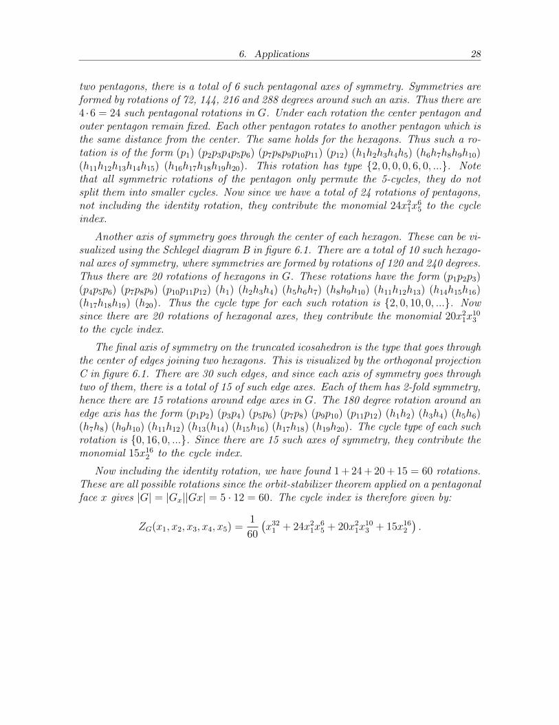
The first, and most tedious task, is finding the cycle index. A truncated icosahedronconsists of 12 pentagons and 20 hexagons. The graphical representations in figure 6.1help to visualize the truncated icosahedron. Each of the three graphs is centered at adifferent type of axis of rotational symmetry.

A B C

Fig. 6.1: The truncated icosahedron centered at the three differenttypes of axes of rotational symmetry. A and B are Schlegeldiagrams and C is an orthogonal projection.

To find the cycle index, we do not need to find all elements in G, it is sufficientto know their types. The type of the identity rotation is clearly {32, 0, ...}. An axisof symmetry goes through the center of each pentagon, as shown in graph A of figure6.1. Since there are 12 pentagons, and each pentagonal axis of symmetry goes through

3 Equivalently a classic soccer ball or buckminsterfullerene molecule.

6. Applications 28

two pentagons, there is a total of 6 such pentagonal axes of symmetry. Symmetries areformed by rotations of 72, 144, 216 and 288 degrees around such an axis. Thus there are4 ·6 = 24 such pentagonal rotations in G. Under each rotation the center pentagon andouter pentagon remain fixed. Each other pentagon rotates to another pentagon which isthe same distance from the center. The same holds for the hexagons. Thus such a ro-tation is of the form (p1) (p2p3p4p5p6) (p7p8p9p10p11) (p12) (h1h2h3h4h5) (h6h7h8h9h10)(h11h12h13h14h15) (h16h17h18h19h20). This rotation has type {2, 0, 0, 0, 6, 0, ...}. Notethat all symmetric rotations of the pentagon only permute the 5-cycles, they do notsplit them into smaller cycles. Now since we have a total of 24 rotations of pentagons,not including the identity rotation, they contribute the monomial 24x21x

65 to the cycle

index.

Another axis of symmetry goes through the center of each hexagon. These can be vi-sualized using the Schlegel diagram B in figure 6.1. There are a total of 10 such hexago-nal axes of symmetry, where symmetries are formed by rotations of 120 and 240 degrees.Thus there are 20 rotations of hexagons in G. These rotations have the form (p1p2p3)(p4p5p6) (p7p8p9) (p10p11p12) (h1) (h2h3h4) (h5h6h7) (h8h9h10) (h11h12h13) (h14h15h16)(h17h18h19) (h20). Thus the cycle type for each such rotation is {2, 0, 10, 0, ...}. Nowsince there are 20 rotations of hexagonal axes, they contribute the monomial 20x21x

103

to the cycle index.

The final axis of symmetry on the truncated icosahedron is the type that goes throughthe center of edges joining two hexagons. This is visualized by the orthogonal projectionC in figure 6.1. There are 30 such edges, and since each axis of symmetry goes throughtwo of them, there is a total of 15 of such edge axes. Each of them has 2-fold symmetry,hence there are 15 rotations around edge axes in G. The 180 degree rotation around anedge axis has the form (p1p2) (p3p4) (p5p6) (p7p8) (p9p10) (p11p12) (h1h2) (h3h4) (h5h6)(h7h8) (h9h10) (h11h12) (h13(h14) (h15h16) (h17h18) (h19h20). The cycle type of each suchrotation is {0, 16, 0, ...}. Since there are 15 such axes of symmetry, they contribute themonomial 15x162 to the cycle index.

Now including the identity rotation, we have found 1 + 24 + 20 + 15 = 60 rotations.These are all possible rotations since the orbit-stabilizer theorem applied on a pentagonalface x gives |G| = |Gx||Gx| = 5 · 12 = 60. The cycle index is therefore given by:

ZG(x1, x2, x3, x4, x5) =1

60

(x321 + 24x21x

65 + 20x21x

103 + 15x162

).

6. Applications 29

Applying PET with weights B = black and W = white gives the CGF

F (B,W ) = ZG(B +W,B2 +W 2, ..., B5 +W 5)

=1

60((B +W )32 + 24(B +W )2(B5 +W 5)6 + 20(B +W )2(B3 +W 3)10+

15(B2 +W 2)16)

= B32 + 2B31W + 13B30W 2 + 86B29W 3 + 636B28W 4 + 3362B27W 5+

15263B26W 6 + 56130B25W 7 + 175775B24W 8 + 467520B23W 9+

1076382B22W 10 + 2150460B21W 11 + 3765292B20W 12 + 5789700B19W 13+

7860190B18W 14+ 9428804B17W 15+ 10021408B16W 16 + 9428804B15W 17+

7860190B14W 18+ 5789700B13W 19+ 3765292B12W20+2150460B11W 21+

1076382B10W 22 + 467520B9W 23 + 175775B8W 24 + 56130B7W 25+

15263B6W 26 + 3362B5W 27 + 636B4W 28 + 86B3W 29 + 13B2W 30+

2BW 31 +W 32.

Reading off the coefficient of the term B12W 20 gives 3,765,292 different ways to colorthe truncated icosahedron such that 12 faces are black and 20 faces are white.

To find the general formula for the distinct n-colorings of the truncated icosahedronunder rotations, we simply substitute n into the cycle index:

ZG(n, n, ..., n) =1

60

(n32 + 15n16 + 20n12 + 24n8

).

The total number of different 2-colorings is thus given by

1

60(232 + 15 · 216 + 20 · 212 + 24 · 28) = 71, 600, 640.

6.2 Number Theory

In number theory PET has been used to generalize various famous theorems, includingthose of Wilson, Gauss, Fermat and Euler. This work was done by Chong-Yun Chaoand published in the Journal of Number Theory in 1982 [1].4 A generalization of bothFermat’s theorem and Gauss’ theorem is presented in this section.

The theorems of Fermat and Gauss are stated as follows:

Theorem 6.5. (Fermat’s Little Theorem) If p is prime and p does not divide a, then

ap−1 ≡ 1 mod p. (6.6)

If p is prime, then for every integer a

ap ≡ a mod p. (6.7)

4 Chao used a generalization of PET known as De Bruijn’s Theorem.

6. Applications 30

Theorem 6.6. (Gauss’ Theorem) If n is a positive integer, then∑d|n

φ(d) = n. (6.8)

These theorems are both generalized in the following theorem:

Theorem 6.7. Let a and n be positive integers. Then∑d|n

φ(d)an/d ≡ 0 mod n. (6.9)

Proof. Let X = {1, ..., n}, Y = {1, ..., a} and let the cyclic group Cn act on X. Now ifwe assign the weight w(y) = 1 to each element in Y , by PET we get the CGF:

ZCn(a, a, ..., a) =1

n

∑d|n

φ(d)an/d. (6.10)

Since the CGF gives the total number of configurations, which is a positive integer, weknow that the RHS of 6.10 is a positive integer. It follows that∑

d|n

φ(d)an/d ≡ 0 mod n.

Example 6.8. If a = 3 and n = 8, then we have∑d|8

φ(d)38/d = φ(1)38 + φ(2)34 + φ(4)32 + φ(8)3

= 6672 = 8 · 834 ≡ 0 mod 8.

Now we show how Fermat’s Little Theorem follows from theorem 6.7. Letting p bea prime and n = p in theorem 6.7 means

1

p

∑d|p

φ(d)ap/d =1

p(φ(1)ap + φ(p)a) =

1

p(ap − a) + a (6.11)

is a positive integer, say k. It follows that ap − a = (k − a)p, i.e. ap ≡ a mod p, whichis equation 6.7. If a and p are relatively prime, then it also holds that ap−1 ≡ 1 modp, which is equation 6.6. This is precisely Fermat’s Little Theorem.

Gauss’ theorem is also a simple consequence of theorem 6.7. Letting a = 1 inequation 6.10 gives ∑

d|n

φ(d) ≡ 0 mod n.

6. Applications 31

This means that for some positive integer k we have

1

n

∑d|n

φ(d) = k.

Since a = 1, there is only one possible configuration on Y X , so k = 1. Thus∑d|n

φ(d) = n

which is equation 6.8 and theorem 6.6 holds.

6.3 Graph Theory

The first application of Polya’s enumeration theorem was in graph theory. Polya himselftreated his 1937 paper as a continuation of Cayley’s work on the enumeration of trees.[7]Since then, PET has been applied to enumerate many types of graphs with specifiedconditions. Some of these include labeled, rooted, connected, bipartite, and euleriangraphs, along with rooted trees, free trees, and tree-like structures.[4] In this sectionwe present how PET has been used in enumerating isomorphism classes of rooted treesand (v,e)-graphs. Many of the enumeration techniques for specific types of trees orgraphs depend on, or are variations of, these two results.[4]

6.3.1 Isomorphism Classes of Rooted Trees

Trees are connected graphs which do not contain cycles. The order p of a tree is thenumber of vertices in the tree. The number of edges stemming from a vertex is knownas the degree of the vertex. In a rooted tree, one of the vertices is designated as theroot. The tree is said to be labeled if each of its vertices has associated with it aunique positive integer less than or equal to p. Otherwise it is said to be unlabeled.Cayley proved that the number of labeled rooted p-trees is given by pp−2.[4] The caseof unlabeled p-trees, however, is much more difficult. We seek a generating functionT (x) which enumerates the non-isomorphic unlabeled rooted trees, i.e.

T (x) =∞∑p=0

Tpxp (6.12)

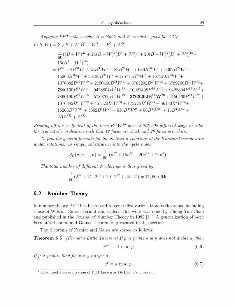
where Tp is the number of rooted trees of order p. The first few rooted trees are listedbelow in figure 6.2 .

6. Applications 32

Fig. 6.2: The rooted trees up to order 3.

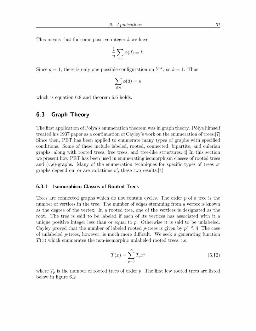
We begin by enumerating the rooted trees which have a root of degree n. Givena set with n rooted trees, a new rooted tree can be formed by adding a vertex andjoining it to the roots of the trees in the set of n rooted trees. This new tree has a rootwith degree n. The symmetric group Sn can then be used to permute the n subtreesstemming from the new root. Figure 6.3 illustrates this method of generating newrooted trees. All trees with a root of degree n can clearly be formed in this manner.

Fig. 6.3: Forming a new rooted tree from a set of 3 rooted trees.

In order to enumerate the trees with a root of degree n we let X = {1, ..., n} andY be the set of all rooted trees.5 To each rooted tree in Y we assign its weight tobe xk, where k is the number of vertices it contains. Summing over all weights ofelements in Y yields T (x). Thus applying PET gives the CGF as a recursive formulaT (x) = ZSn(T (x), T (x2), T (x3), ...), where the coefficients of each xk gives the numberof trees with k+ 1 vertices and a root of degree n. Multiplying through by x accountsfor the new roots. Then summing over all n gives

T (x) = x∞∑n=1

ZSn(T (x), T (x2), T (x3), ...) (6.13)

The following recursive formula for Tp+1 in terms of T1, ..., Tp can then be derived usingequation 6.13 and various identities:6

5 PET can be formulated to allow an infinite set of ’colors’.[4]6 For details of derivations see [4, p.52-54]

6. Applications 33

Tp+1 = p−1p∑

k=1

∑d|k

dTd

Tp−k+1 (6.14)

The first 26 values of Tp are given by Harary and Palmer in [4, Appendix I]:7

p Tp p Tp p Tp1 1 10 719 19 4 688 6762 1 11 1 842 20 12 826 2283 2 12 4 766 21 35 221 8324 4 13 12 486 22 97 055 1815 9 14 32 973 23 268 282 8556 20 15 87 811 24 743 724 9847 48 16 235 381 25 2 067 174 6458 115 17 634 847 26 5 759 636 5109 286 18 1 721 159

Tab. 6.1: The number of rooted trees with p vertices.

6.3.2 Isomorphism Classes of (v,e) Graphs

A (v, e) graph is a graph with v vertices and e edges. Two (v, e) graphs are said to beisomorphic if there is an edge-preserving bijection between them. We seek a generatingfunction Gv(x) with the coefficient of each xe giving the number of non-isomorphic (v, e)graphs gv,e, i.e.

Gv(x) =

(v2)∑

e=0

gv,exe. (6.15)

We let V be the set of v vertices, and V (2) be the set of all possible 2-subsets, oredges, of V . Two graphs G and G′ with v vertices are isomorphic if a permutation ofthe vertices exists that maps the edges of G to the edges of G′. The symmetric groupSv is the appropriate permutation group on the vertices of a graph and it induces anatural group of permutations S

(2)v on the edges known as the pair group of Sv. An

element σ ∈ Sv induces the element σ′ ∈ S(2)v by the equation

σ′(x, y) = (σ(x), σ(y)), for each (x, y) ∈ V (2).

The pair group S(2)v thus acts on the set of edges V (2), and two graphs are isomorphic

if and only if there exists a permutation in S(2)v that maps the edges of one graph to the

7 The sequence is also found in the OEIS as sequence A000081.

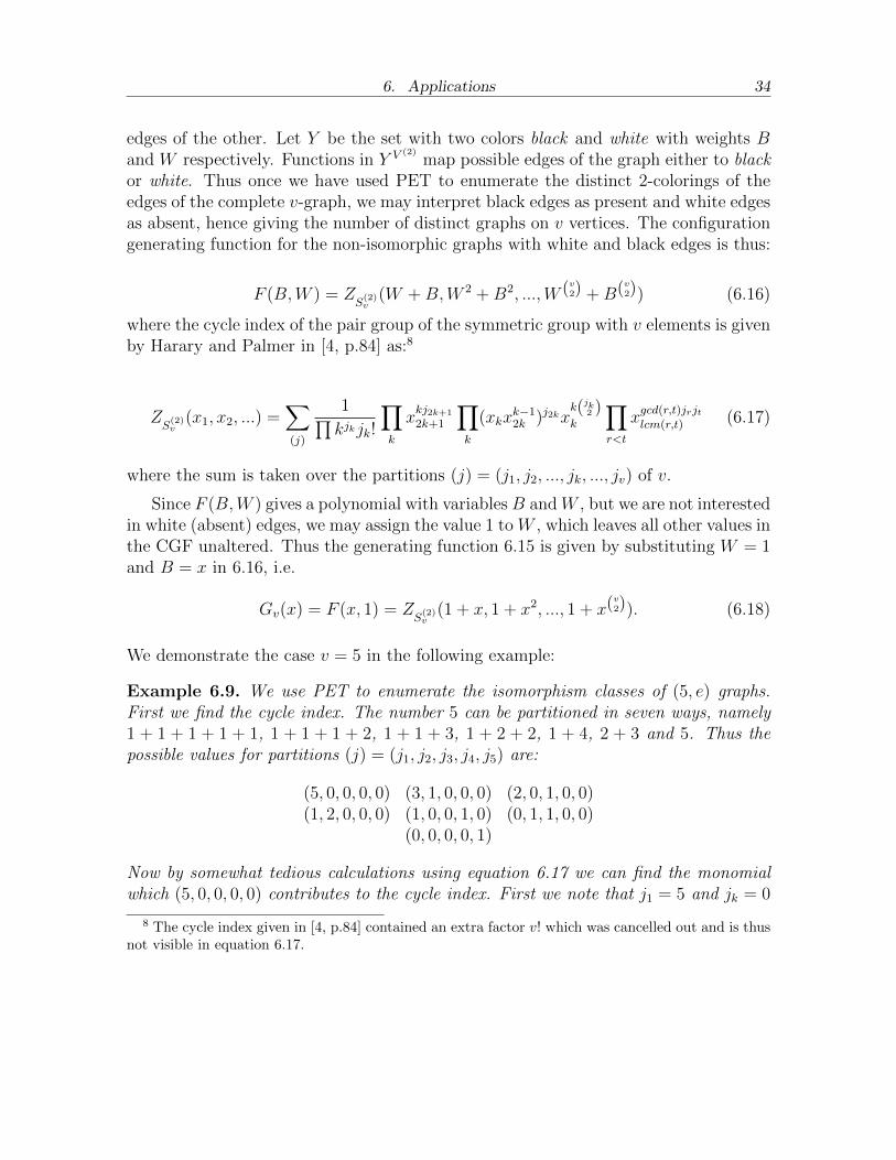
6. Applications 34

edges of the other. Let Y be the set with two colors black and white with weights Band W respectively. Functions in Y V (2)

map possible edges of the graph either to blackor white. Thus once we have used PET to enumerate the distinct 2-colorings of theedges of the complete v-graph, we may interpret black edges as present and white edgesas absent, hence giving the number of distinct graphs on v vertices. The configurationgenerating function for the non-isomorphic graphs with white and black edges is thus:

F (B,W ) = ZS(2)v

(W +B,W 2 +B2, ...,W (v2) +B(v

2)) (6.16)

where the cycle index of the pair group of the symmetric group with v elements is givenby Harary and Palmer in [4, p.84] as:8

ZS(2)v

(x1, x2, ...) =∑(j)

1∏kjkjk!

∏k

xkj2k+1

2k+1

∏k

(xkxk−12k )j2kx

k(jk2 )

k

∏r<t

xgcd(r,t)jrjtlcm(r,t) (6.17)

where the sum is taken over the partitions (j) = (j1, j2, ..., jk, ..., jv) of v.

Since F (B,W ) gives a polynomial with variables B andW , but we are not interestedin white (absent) edges, we may assign the value 1 to W , which leaves all other values inthe CGF unaltered. Thus the generating function 6.15 is given by substituting W = 1and B = x in 6.16, i.e.

Gv(x) = F (x, 1) = ZS(2)v

(1 + x, 1 + x2, ..., 1 + x(v2)). (6.18)

We demonstrate the case v = 5 in the following example:

Example 6.9. We use PET to enumerate the isomorphism classes of (5, e) graphs.First we find the cycle index. The number 5 can be partitioned in seven ways, namely1 + 1 + 1 + 1 + 1, 1 + 1 + 1 + 2, 1 + 1 + 3, 1 + 2 + 2, 1 + 4, 2 + 3 and 5. Thus thepossible values for partitions (j) = (j1, j2, j3, j4, j5) are:

(5, 0, 0, 0, 0) (3, 1, 0, 0, 0) (2, 0, 1, 0, 0)(1, 2, 0, 0, 0) (1, 0, 0, 1, 0) (0, 1, 1, 0, 0)

(0, 0, 0, 0, 1)

Now by somewhat tedious calculations using equation 6.17 we can find the monomialwhich (5, 0, 0, 0, 0) contributes to the cycle index. First we note that j1 = 5 and jk = 0

8 The cycle index given in [4, p.84] contained an extra factor v! which was cancelled out and is thusnot visible in equation 6.17.

6. Applications 35

when k 6= 1. Thus

1∏kjkjk!

=1

(155!)(200!)(300!)(400!)(500!)=

1

(155!)∏k

xkj2k+1

2k+1 = (x1·03 )(x2·05 )(x3·07 )(x4·09 )(x5·011 ) = 1

∏k

(xkxk−12k )j2kx

k(jk2 )

k = ((x1x02)

0x1·(5

2)1 ) · ((x2x14)0x

2·(02)

2 ) · ((x3x26)0x3·(0

2)3 ) ·

((x4x38)

0x4·(0

2)4 ) · ((x5x104)0x

5·(02)

5 ) = x(52)

1∏r<t

xgcd(r,t)jrjtlcm(r,t) = (x0lcm(1,2))(x

0lcm(1,3))(x

0lcm(2,3))(x

0lcm(1,4)) · · · (x0lcm(4,5)) = 1

Hence the partition (5, 0, 0, 0, 0) contributes to the cycle index the term:

1

155!(1)(x

(52)

1 )(1) =1

120x101

Similarly (3, 1, 0, 0, 0) contributes the term:

1

133!211!(x03x

05)((x1x

02)

1x(32)

1 (x2x4)0x

2·(12)

2 )(x3·gcd(1,2)lcm(1,2) ) =

1

12x41x

32

(2, 0, 1, 0, 0) contributes the term:

1

311!122!(x13)(x1x

02)

0x(22)

1 (x2x4)0x

(02)

2 (x2·gcd(1,3)lcm(1,3) ) =

1

6x1x

33


1

111!222!(x03x

05)(x1x

02)

2x(12)

1 (x2x34)

0x2(2

2)2 (x

gcd(1,2)·2lcm(1,2) ) =

1

8x21x

42


1

111!411!(x03x

05)(x1x

02)

0x(12)

1 (x2x4)1x

4(12)

4 (xgcd(4,1)lcm(4,1)) =

1

4x2x

24


1

211!311!(x13)(x1x

02)

1x(02)

1 (x2x14)

0(x2)2(1

2)(xgcd(2,3)lcm(2,3)) =

1

6x1x3x6


1

511!(x5)

2(x5(1

2)5 )(1) =

1

5x25

6. Applications 36

The cycle index is thus given by:9

ZS(2)5

=1

120

(x101 + 10x41x

32 + 20x1x

33 + 15x21x

42 + 30x2x

24 + 20x1x3x6 + 24x25

)Now by equation 6.18 we have

G5(x) = ZS(2)5

(1 + x, 1 + x2, ..., 1 + x6)

=1

120

((1 + x)10 + 10(1 + x)4(1 + x2)3 + 20(1 + x)(1 + x3)3 +

15(1 + x)2(1 + x2)4 + 30(1 + x2)(1 + x4)2 +

20(1 + x)(1 + x3)(1 + x6) + 24(1 + x5)2)

= 1 + x+ 2x2 + 4x3 + 6x4 + 6x5 + 6x6 + 4x7 + 2x8 + x9 + x10

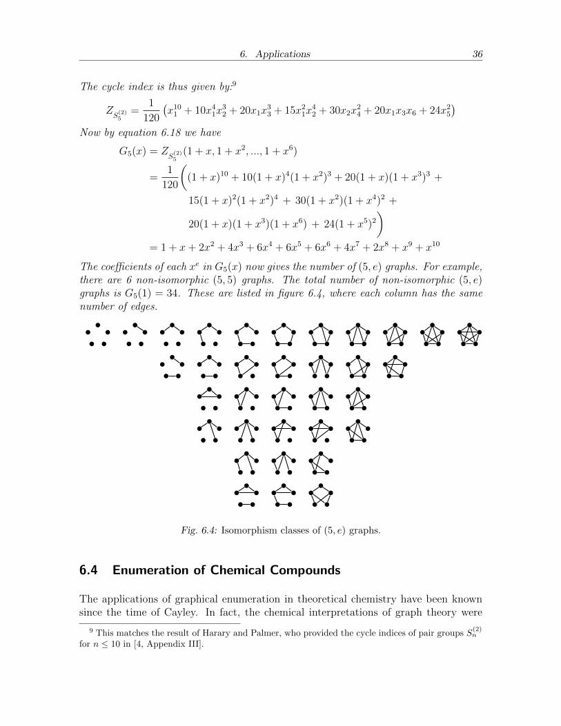
The coefficients of each xe in G5(x) now gives the number of (5, e) graphs. For example,there are 6 non-isomorphic (5, 5) graphs. The total number of non-isomorphic (5, e)graphs is G5(1) = 34. These are listed in figure 6.4, where each column has the samenumber of edges.

Fig. 6.4: Isomorphism classes of (5, e) graphs.

6.4 Enumeration of Chemical Compounds

The applications of graphical enumeration in theoretical chemistry have been knownsince the time of Cayley. In fact, the chemical interpretations of graph theory were

9 This matches the result of Harary and Palmer, who provided the cycle indices of pair groups S(2)n

for n ≤ 10 in [4, Appendix III].

6. Applications 37

largely what motivated his research in the enumeration of trees. Polya, continuing inCayley’s footsteps, spent a considerable amount of his groundbreaking 1937 paper onthe applications of PET in chemical enumeration.[7]

In chemistry, there is generally no bijective correspondence between the set ofmolecules and the set of chemical formulas. A chemical formula may represent morethan one molecule, whose arrangement of atoms differs in space. Such molecules withthe same chemical formula but different chemical structures are known as isomers.PET can be used to enumerate different types of isomers.[7]

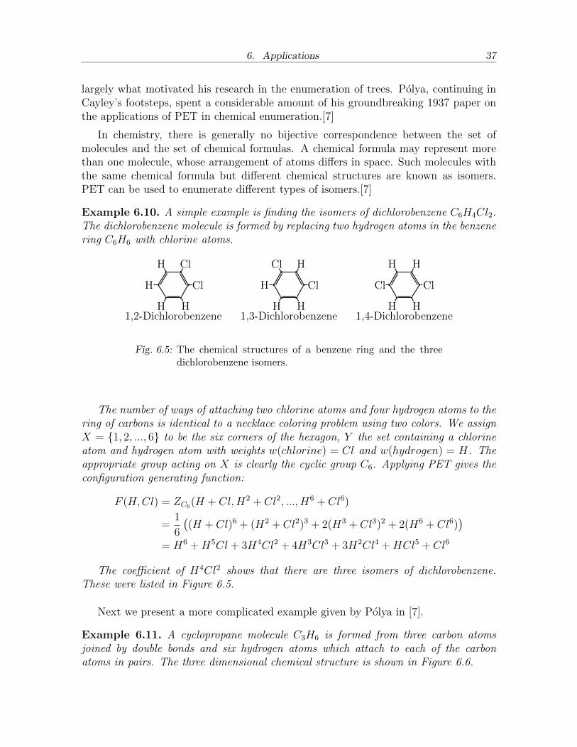
Example 6.10. A simple example is finding the isomers of dichlorobenzene C6H4Cl2.The dichlorobenzene molecule is formed by replacing two hydrogen atoms in the benzenering C6H6 with chlorine atoms.

Cl

ClH

H

H H1,2-Dichlorobenzene

Cl

HCl

H


Cl

HH

Cl


Fig. 6.5: The chemical structures of a benzene ring and the threedichlorobenzene isomers.

The number of ways of attaching two chlorine atoms and four hydrogen atoms to thering of carbons is identical to a necklace coloring problem using two colors. We assignX = {1, 2, ..., 6} to be the six corners of the hexagon, Y the set containing a chlorineatom and hydrogen atom with weights w(chlorine) = Cl and w(hydrogen) = H. Theappropriate group acting on X is clearly the cyclic group C6. Applying PET gives theconfiguration generating function:

F (H,Cl) = ZC6(H + Cl,H2 + Cl2, ..., H6 + Cl6)

=1

6

((H + Cl)6 + (H2 + Cl2)3 + 2(H3 + Cl3)2 + 2(H6 + Cl6)

)= H6 +H5Cl + 3H4Cl2 + 4H3Cl3 + 3H2Cl4 +HCl5 + Cl6

The coefficient of H4Cl2 shows that there are three isomers of dichlorobenzene.These were listed in Figure 6.5.

Next we present a more complicated example given by Polya in [7].

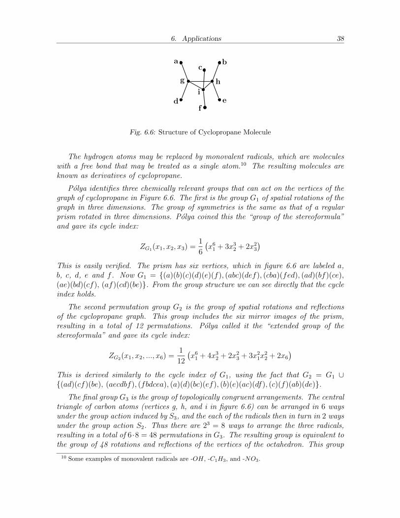
Example 6.11. A cyclopropane molecule C3H6 is formed from three carbon atomsjoined by double bonds and six hydrogen atoms which attach to each of the carbonatoms in pairs. The three dimensional chemical structure is shown in Figure 6.6.

6. Applications 38

a

d

b

e

c

f

g h

i

Fig. 6.6: Structure of Cyclopropane Molecule

The hydrogen atoms may be replaced by monovalent radicals, which are moleculeswith a free bond that may be treated as a single atom.10 The resulting molecules areknown as derivatives of cyclopropane.

Polya identifies three chemically relevant groups that can act on the vertices of thegraph of cyclopropane in Figure 6.6. The first is the group G1 of spatial rotations of thegraph in three dimensions. The group of symmetries is the same as that of a regularprism rotated in three dimensions. Polya coined this the “group of the stereoformula”and gave its cycle index:

ZG1(x1, x2, x3) =1

6

(x61 + 3x32 + 2x23

)This is easily verified. The prism has six vertices, which in figure 6.6 are labeled a,b, c, d, e and f . Now G1 = {(a)(b)(c)(d)(e)(f), (abc)(def), (cba)(fed), (ad)(bf)(ce),(ae)(bd)(cf), (af)(cd)(be)}. From the group structure we can see directly that the cycleindex holds.

The second permutation group G2 is the group of spatial rotations and reflectionsof the cyclopropane graph. This group includes the six mirror images of the prism,resulting in a total of 12 permutations. Polya called it the “extended group of thestereoformula” and gave its cycle index:

ZG2(x1, x2, ..., x6) =1

12

(x61 + 4x32 + 2x23 + 3x21x

22 + 2x6

)This is derived similarly to the cycle index of G1, using the fact that G2 = G1 ∪{(ad)(cf)(be), (aecdbf), (fbdcea), (a)(d)(bc)(ef), (b)(e)(ac)(df), (c)(f)(ab)(de)}.

The final group G3 is the group of topologically congruent arrangements. The centraltriangle of carbon atoms (vertices g, h, and i in figure 6.6) can be arranged in 6 waysunder the group action induced by S3, and the each of the radicals then in turn in 2 waysunder the group action S2. Thus there are 23 = 8 ways to arrange the three radicals,resulting in a total of 6 ·8 = 48 permutations in G3. The resulting group is equivalent tothe group of 48 rotations and reflections of the vertices of the octahedron. This group

10 Some examples of monovalent radicals are -OH, -C1H3, and -NO3.

6. Applications 39

was referred to by Polya as the “group of the structural formula”. He derived it bysubstituting the cycle index of S2 into the cycle index of S3, producing the cycle index:

ZG3(x1, x2, ..., x6) = ZS3(ZS2(x1, x2), ZS2(x2, x4), ZS2(x3, x6))

=1

6(ZS2(x1, x2)

3 + 3ZS2(x1, x2)ZS2(x2, x4) + 2ZS2(x3, x6))

=1

6(1

2(x21 + x2))

3 + 3 · 1

2(x21 + x2) ·

1

2(x22 + x4) + 2 · 1

2(x23 + x6))

=1

48

(x61 + 3x41x2 + 9x21x

22 + 6x4x

21 + 7x32 + 6x4x2 + 8x23 + 8x6

)Now, for each type of symmetry, we can find the number of different derivatives of

cyclopropane of the form C3XkYlZm, where k+ l+m = 6 and X, Y and Z are differentindependent radicals.11 Applying PET with the three cycle indices above and weightsw(X) = x, w(Y ) = y and w(Z) = z gives configuration generating functions:12

F1(x, y, z) = ZG1(x+ y + z, x2 + y2 + z2, x3 + y3 + z3)

= x6 + x5y + x5z + 4x4y2 + 5x4yz + 4x4z2 + 4x3y3 + 10x3y2z + 10x3yz2+

4x3z3 + 4x2y4 + 10x2y3z + 18x2y2z2 + 10x2yz3 + 4x2z4 + xy5 + 5xy4z+

10xy3z2 + 10xy2z3 + 5xyz4 + xz5 + y6 + y5z + 4y4z2 + 4y3z3 + 4y2z4+

yz5 + z6

F2(x, y, z) = ZG2(x+ y + z, x2 + y2 + z2, ..., x6 + y6 + z6)




yz5 + z6

F3(x, y, z) = ZG3(x+ y + z, x2 + y2 + z2, ..., x6 + y6 + z6)




yz5 + z6

Reading off the coefficients of the term x4y2 gives the number of different derivativesof cyclopropane of the form C3X4Y2. There are four unique derivatives under spatialrotations, three unique derivatives if mirror images are disregarded, and two uniquederivatives if spatial arrangement is disregarded.

11 “Independent means that XkYlZm and Xk′Yl′Zm′ have the same molecular structure only ifk = k′, l = l′ and m = m′.”[7]

12 Polya only gives the first few terms of each polynomial, the rest were calculated using Maple 2015.

7. Conclusion 40

7 Conclusion

In the previous chapter we saw the power and generality of Polya’s Enumeration The-orem as it was applied to various different applications. Problems which would beextremely tedious using Burnside’s lemma, such as coloring the truncated icosahedron,were solved by PET with relative ease. The enumeration of unlabeled rooted trees wasdone by formulating PET into a recursive equation. The properties of the cycle indexfor the cyclic group proved to have connections to number theory.

Despite its generality, PET does have certain limitations. Often the main difficultyin applying it is finding the cycle index, as it can be something as unwieldy as for thepair group in equation 6.17. It is also not hard to pose problems which are seeminglyPolya type problems but cannot be solved by PET. For example, PET requires thechoice of colors to be independent of one another, i.e. the choice of one color does notaffect the choice of another. Given a necklace coloring problem using six beads andthree colors, if we add the restriction that two adjacent beads cannot have the samecolor, then the colorings are no longer independent. This problem can no longer besolved by PET, but can in fact be done by resorting back to Burnside’s lemma. PEThas been generalized further, and a notable such generalization was done by De Bruijnin 1959. Considering again example 6.3, we have the group of rotations G acting onthe set of faces of the cube X, and the set of colors Y . Suppose now that we considertwo colorings equivalent not only if one can be obtained from the other by rotations,but also if it can be obtained by interchanging the colors of the faces. Thus in additionto G acting on X, we have a group H acting on the set of colors Y . In such a situationDe Bruijn’s generalization can be used to enumerate the configurations.[7]

Limitations and generalizations aside, PET itself solved a whole class of enumera-tion problems in a single unifying theorem, making a significant contribution to com-binatorial mathematics. With its wide range of applications, PET has proved to be avaluable tool in the discrete mathematician’s toolbox.

Bibliography 41

Bibliography

[1] Chao, Chong-Yun. ”Generalizations of Theorems of Wilson, Fermat and Euler.”Journal of Number Theory 15.1 (1982): 95-114. Web. 19 Aug. 2015.

[2] De Bruijn, Nicolaas G. ”Polya’s Theory of Counting.” Applied CombinatorialMathematics. By Edwin F. Beckenbach and George Polya. New York: J. Wiley,1964. N. pag. Print.

[3] Graver, Jack E., and Mark E. Watkins. Combinatorics with Emphasis on theTheory of Graphs. New York: Springer-Verlag, 1977. 322-28. Print.

[4] Harary, Frank, and Edgar M. Palmer. Graphical Enumeration. New York: Aca-demic, 1973. Print.

[5] Hungerford, Thomas W. Algebra. New York: Springer, 1974. Print.

[6] Lidl, Rudolf, and Gunter Pilz. Applied Abstract Algebra. New York: Springer-Verlag, 1984. Print.

[7] Polya, George, and Ronald C. Read. Combinatorial Enumeration of Groups,Graphs, and Chemical Compounds. New York: Springer-Verlag, 1987. Print.

[8] Rotman, Joseph J. An Introduction to the Theory of Groups. New York: Springer-Verlag, 1995. Print.

[9] Wilf, Herbert S. Generatingfunctionology. San Diego: Academic, 1994. Print.

[10] Wussing, Hans. The Genesis of the Abstract Group Concept: A Contribution tothe History of the Origin of Abstract Group Theory. New York: Courier Dover,2007. Print.

POLYA’S ENUMERATION THEOREM AND ITS APPLICATIONS …

Documents

Transcript of POLYA’S ENUMERATION THEOREM AND ITS APPLICATIONS …