Pollution Motivates Hope-Seeking Behavior
42
1 Pollution Motivates Hope-Seeking Behavior Shaoshuai Li Jaimie W. Lien Jia Yuan University of Macau The Chinese University of Hong Kong University of Macau Current Version: February 18 th , 2021 Initial Version: April 1, 2018 Abstract: 1 In developing countries around the world, air pollution remains a serious issue which has possible unexpected influences on a variety of human decisions. Using a rich panel data structure with air quality observations at a daily frequency, we discover a robust positive relationship between air pollution and lottery gambling and investigate the mechanism for this relationship. Psychological influences account for a significant proportion of this positive relationship, as evidenced by a robust significant effect of reduced visibility conditions on lottery ticket purchases. However, chemical components of AQI (Air Quality Index) are also significantly responsible for the decision to purchase tickets, particularly sulfur dioxide (SO2), which suggests a larger impact of the early particulate formation process on human behavior than previously considered in most studies. We further show that limited attention to information about air quality levels is a significant factor, by identifying discontinuous jumps in lottery ticket purchases at government provided color-coded AQI transition thresholds around the “Moderate” or “Unhealthy” level, implying that the increase in ticket purchases is cognitively-driven. Finally, adverse regional economic conditions, namely the unemployment rate, significantly enhances the appeal of lotteries under polluted conditions. Altogether, our findings suggest a significant conscious appeal of lottery tickets as a hope-seeking device under negative environmental conditions. JEL Codes: D01, D81, Q53 Keywords: air pollution, AQI, visibility, gambling behavior, limited attention, regional economic conditions, avoidance 1 Li: Department of Economics, Faculty of Business Administration, University of Macau, [email protected]; Lien: Department of Decision Sciences and Managerial Economics, The Chinese University of Hong Kong, [email protected] ; Yuan: Department of Economics, Faculty of Business Administration, University of Macau, [email protected] .
Transcript of Pollution Motivates Hope-Seeking Behavior
1
Pollution Motivates Hope-Seeking Behavior
Shaoshuai Li Jaimie W. Lien Jia Yuan
University of Macau The Chinese University of
Hong Kong
University of Macau
Current Version: February 18th, 2021
Initial Version: April 1, 2018
Abstract:1
In developing countries around the world, air pollution remains a serious issue which has possible unexpected
influences on a variety of human decisions. Using a rich panel data structure with air quality observations at a daily
frequency, we discover a robust positive relationship between air pollution and lottery gambling and investigate the
mechanism for this relationship. Psychological influences account for a significant proportion of this positive relationship,
as evidenced by a robust significant effect of reduced visibility conditions on lottery ticket purchases. However, chemical
components of AQI (Air Quality Index) are also significantly responsible for the decision to purchase tickets, particularly
sulfur dioxide (SO2), which suggests a larger impact of the early particulate formation process on human behavior than
previously considered in most studies. We further show that limited attention to information about air quality levels is a
significant factor, by identifying discontinuous jumps in lottery ticket purchases at government provided color-coded AQI
transition thresholds around the “Moderate” or “Unhealthy” level, implying that the increase in ticket purchases is
cognitively-driven. Finally, adverse regional economic conditions, namely the unemployment rate, significantly enhances
the appeal of lotteries under polluted conditions. Altogether, our findings suggest a significant conscious appeal of lottery
tickets as a hope-seeking device under negative environmental conditions.
JEL Codes: D01, D81, Q53
Keywords: air pollution, AQI, visibility, gambling behavior, limited attention, regional economic conditions, avoidance
1 Li: Department of Economics, Faculty of Business Administration, University of Macau, [email protected];
Lien: Department of Decision Sciences and Managerial Economics, The Chinese University of Hong Kong,
Yuan: Department of Economics, Faculty of Business Administration, University of Macau, [email protected] .
2
1. Introduction
Increasing attention has been drawn to the effects of air pollution exposure on human behavior in recent years.
While early on social scientists recognized the need to understand how pollution could affect economic behavior such as
worker performance (ex. Lagercrantz, et al, 2000), a recent resurgence of interest in the negative impacts of air pollution
on mental health (Zhang, Zhang and Chen, 2017), cognitive performance (Zhang, Chen and Zhang, 2018), worker
productivity (Graff Zivin and Neidell, 2012; Chang, Graff Zivin, Gross, and Neidell, 2016; Lichter, Pestel and Sommer,
2017; He, Liu and Salvo, 2019; Chang, Graff Zivin, and Neidell, forthcoming), and consumption behavior (Barwick, Li,
Lin and Zou, 2019) has grown due to the phenomenon of heavy air pollution in the developing world.2
Lottery gambling has also been a topic of significant interest, both from the perspective of decision-making (ex.
Lien and Yuan, 2015a, 2015b; Lien, Yuan and Zheng, 2017, among others) and from a policy perspective (ex. Perez and
Humphreys, 2011; Humphreys and Perez, 2012, among others).3 In this study, we demonstrate a robust relationship
between air pollution and lottery gambling, and conduct analysis in order to understand the detailed mechanisms for this
significant positive relationship. Medical research has focused on the impact of various chemical reactions on biological
functioning, while the social sciences have focused mostly on non-biological, reasoning-based motives for human
decisions. These fields have not frequently intersected to provide an understanding of how specific human decisions such
as risk-taking and consumer purchase decisions could be affected by the presence of the chemical composition in the
environment. To begin understanding the mechanism behind air pollution’s positive effect on lottery sales, we use an
econometric approach to examine the combination of factors which could serve to potentially enhance the appeal of lottery
ticket purchase under polluted conditions.
By examining lottery sales in the days leading up to the thrice weekly lottery draw of Union Lotto, China’s official
lottery game which is also the most popular lottery game in China, we find that higher air pollution levels lead to
significantly higher lottery ticket sales.4 The effect is robust across both northern and southern regions of China and is
generally driven by the autumn and winter seasons of the year. Examining the simultaneous effects of each component of
AQI, we find that the primary AQI component responsible for this increase in lottery purchase is sulfur dioxide (SO2),
particularly during the autumn months. Most prior studies have focused on the effect of particulate matter (PM 2.5 and
PM 10) on behavior changes (Graff Zivin and Neidell, 2012; Chang, Graff Zivin, Gross, and Neidell, 2016; Lichter, Pestel
and Sommer, 2017; Zhang, Zhang and Chen, 2017; Zhang, Chen and Zhang, 2018; He, Liu and Salvo, 2019; Chang, Graff
Zivin, and Neidell, forthcoming). We find that although each official component of AQI indeed contributes significantly
positively to the increased lottery ticket purchase when examined separately, when controlling for levels of the different
AQI components, the frequently studied particulate matter measure (PM2.5) does not have a significant positive effect,
while SO2 in fact does. Since SO2 is understood to be a predecessor to particulate matter, the result suggests that behavior
could be influenced by air pollution earlier on in the particulate development process than previously considered.
The overwhelming majority of economic studies regarding pollution’s effect on human behavior focus on
establishing the correlation or causal effect between pollution and particular choices or outcomes.5 However, to our
knowledge, few if any studies attempt to explain the mechanism for the relationship between pollution and behavior. The
mechanisms for pollution’s influence on behavior may be especially important for those domains of interest involving
2 For a more complete listing of pollution-related studies, we refer to Lu (2020) which provides a current review of the existing
literature on the psychological, economic, and social effects of air pollution. 3 We refer to Humphreys and Perez (2013), which provides a detailed survey of the literature on lottery demand. 4 A positive relationship between air pollution and lottery gambling is also supported in an independently conceived study, Chew, Liu
and Salvo (2019), which focuses specifically on establishing a robust causal relationship between particulate matter (PM 2.5) and
purchase of China’s 3D lottery and related games. Our study benefits from their work in establishing a causal relationship between
pollution and gambling behavior, which allows us to focus on the possible mechanisms through which air pollution influences
gambling. However, our study departs substantially from theirs by investigating the potential mechanisms for the positive relationship,
particularly through psychological and economic channels. 5 See also Chew, Huang and Li (2017) which tests the effect of pollution conditions on economic preference parameters in a laboratory
experiment, and Gao, Lien, Wang and Zheng (2019) which examines the effect of pollution on financial analysts’ forecasting
performance.
3
human choice. In the case of choice-based behavior, several potential factors could influence human decisions. The first
and perhaps most obvious of the categories when considering pollution-related behavior is through biological channels.
For example, one or more chemical components of AQI could lead to biological needs (similar to hunger), which
eventually lead the decision-maker, perhaps to some extent involuntarily, to a particular choice. Another potential channel
is through the influence on psychological states through mood, which then lead the decision-maker to a choice. Still
another potential channel is through information provided, which suggests a more cognitive, deliberate choice being made.
Finally, economic conditions could set the psychological state of the decision-maker leading to a disposition for particular
choices. Although this is not an exhaustive list of the possible channels for the effect of pollution on gambling, these are
the main factors that we consider in this paper.
Beyond our basic findings on the relationship between lottery gambling and AQI components, our study examines
three main factors which may drive the pollution-gambling link: 1. Visibility conditions, which are often correlated with
air pollution and can be controlled for in order to assess the chemical versus perceptional impact of air pollutants on
decisions; 2. The role of information provision and limited attention to AQI in the pollution-driven gambling appeal; 3.
How regional economic conditions interact with the decision to purchase lottery tickets on high air pollution days.
First, we use visibility data from the National Oceanic and Atmospheric Administration (NOAA) to assess how
the correlation between high AQI levels and reduced sunlight and air transparency accounts for the relationship between
pollution and gambling behavior. Previous studies have used visibility conditions as a proxy for AQI when official
statistics are unavailable (Du, Li and Yuan, 2014). Utilizing the data period in which the two data series overlap allows
us to decompose the visual effects of air pollution from the air pollution content itself in explaining lottery gambling. Our
baseline estimate suggests that reduced visibility accounts for about 22% of the increase in lottery sales found per AQI
point overall. In other words, reduced visibility due to pollution plays a significant role in individuals’ pollution-driven
desire for lottery gambling - and since actual AQI content is controlled for, this effect may be interpreted as perceptional
or mood-driven in nature.
Secondly, we examine the role of information about AQI and limited attention to AQI levels on lottery purchase.
If the effect of pollution on gambling behavior is purely through a biologically driven channel, then providing information
about AQI should not have a significant impact on the amount of lottery tickets sold. A recent study (Barwick, Li, Lin and
Zou, 2020) however, finds that information provision regarding pollution promotes avoidance behavior. In addition, once
AQI information is provided to individuals, the color-coded categories of pollution intensity should not have a
discontinuous effect on lottery sales, since two different but adjacent color-codings are only a single AQI point away from
one another and are thus only marginally different in terms of actual air quality. If such a discontinuous effect exists, it
suggests that limited attention to the AQI number itself drives individuals to be reliant on color-coded categories in
determining the degree of air pollution present, and in turn, how much they want to buy lottery tickets. We find that indeed,
lottery sales are disproportionately responsive to the AQI number that immediately qualifies as “moderately polluted”
(color code red), which indicates that lottery ticket consumers pay significant attention to pollution rating categories in
considering their lottery ticket purchases. Furthermore, this effect exists only after the public release of daily AQI statistics
and pollution category color coding by the Ministry of Environmental Protection of China (MEP) from year 2013 onward,
which supports the attention mechanism.
Finally, we examine the role of regional economic conditions on the appeal of tickets. Regional unemployment
rates and GDP per capita are both significantly associated with additional lottery sales in terms of their interaction effect
with pollution levels. This provides general support for the idea that an important appeal of lottery tickets is the hope that
they provide to individuals for an appealing future (Ng, 1965).
We note that while it might be considered natural to conjecture that heavy air pollution has an adverse effect on
mental health, cognitive performance, and worker productivity as shown in previous studies, the relationship between air
pollution and lottery gambling may be less intuitive and perhaps more surprising. A negative influence of air pollution on
some of the previously studied domains, such as productivity and cognitive performance, mainly involves passivity on the
part of the decision-maker – ie. polluted conditions may lead individuals to be less proactive or less able in pursuing
mental wellness, cognitive achievement and high productivity. However, for the case of lottery gambling, in order for a
4
significantly positive effect to exist, deliberate action is required on the part of individuals – ie. actively purchasing lottery
tickets that they would not have purchased otherwise.
This finding stands in notable contrast to the more generally negative relationship between air pollution and
consumer activity found in Barwick, Li, Lin and Zou (2019), which found a significant avoidance effect of pollution
information on consumers’ spending behaviors.6 The discrepancy between their results, which utilize credit card data to
assess overall expenditure behaviors, and ours, which focuses on realized lottery demand, indicates that lottery tickets
have a specific appeal to consumers during high pollution periods which does not extend to expenditure and consumption
activity more generally. In other words, based on prior findings on avoidance behavior due to air pollution, our results
imply that there is something indeed different about the appeal of lottery purchase compared to other types of purchases
more generally; it is not merely that pollution enhances the overall utility value of making purchases. Our study focuses
on gaining insights into the psychological mechanism for this appeal of lottery tickets on polluted days.
The paper is organized as follows: Section 2 presents the basic results on AQI and lottery sales, including
robustness checks and decompositions across regions and seasons; Section 3 discusses the relative impacts of visibility
and AQI compound components; Section 4 provides the evidence on information and attention influences on lottery
gambling. Section 5 discusses the relationship between the pollution-lottery effect and regional economic variables.
Section 6 concludes.
2. Basic Results
We collect lottery sales data from the China Welfare Lottery Management Center (CWLM). This dataset contains
provincial level lottery sales for each lottery draw over the period 2005 - 2017.7 Each year has approximately 154 lottery
draws.8 There are 1994 lottery draws in total over our total investigation period and the average amount of lottery ticket
sales per draw is 8,370,689 RMB. We exploit a rich panel data structure across the 31 administrative provinces and nearly
2000 lottery draws, their associated sales and daily AQI data, to assess the relationship between air pollution and lottery
ticket sales.
The AQI data is collected from the Ministry of Environmental Protection of China (MEP). The AQI data starts
from year 2008 and the index values range from 0 to 500. The AQI is determined by the levels of 6 atmospheric pollutants,
namely sulfur dioxide (SO2), nitrogen dioxide (NO2), carbon monoxide (CO), fine particulate matters (PM 2.5 and PM 10)
and ozone (O3).9 According to the standard established by the Ministry of Environmental Protection of China, the AQI
ranges from 0 to 500 and has 6 groups: excellent (0-50), good (51-100), lightly polluted (101-150), moderately polluted
(151-200), heavily polluted (201-300) and severely polluted (larger than 300). Visibility data is collected from the U.S.
National Oceanic and Atmospheric Administration (NOAA) and is expressed in kilometers of visibility.10 Appendix A,
Table A1 displays summary statistics for the main variables in our analysis over the sample period.
To examine the relationship between lottery sales and air pollution, we adopt the following baseline model for
lottery sales based on the province-level panel dataset:
𝑙𝑛(𝑌𝑖𝑡) = 𝛼 + 𝛽ln(𝑋𝑖𝑡) + ρ𝑊𝑖𝑡 + γ𝑖 + 𝛿𝑡 + 휀𝑖𝑡 ,
6 See also Neidell (2009) regarding avoidance behavior on outdoor activities. 7 The Union Lotto has been sold publicly since 16-Feb-2003. Before 1-Jan- 2005, the CWLM only disclosed the national aggregate
level sales data, but not the provincial level data.. 8 For the years of our analysis, the number of lottery draws per year ranged from 152 to 154. Lottery draws take place on each Tuesday,
Thursday and Sunday, with suspension for the annual Spring Festival. 9 Data for the disaggregated components of AQI is available from 2014 onward. For this reason, we focus on data starting from 2014
in those specifications for which we are interested in comparing the effects with AQI components. 10 Visibility data is available from 1960 onward from NOAA.
5
where 𝑌𝑖𝑡 is lottery sales on day t for province i, extrapolated by averaging across the upcoming lottery round.11 𝑋𝑖𝑡 are air
pollution measures. Weather variables 𝑊𝑖𝑡, are included as controls, namely the average local temperature, wind speed,
and an indicator for rain. In addition, we include province fixed effects γ𝑖 , and day-of-week fixed effects𝛿𝑡 , to capture
the provincial-specific characteristics and lottery sales time-specific features, respectively. This allows us to omit control
variables associated with particular provinces and years from the regression, while still accounting for their potential
influences on lottery sales. 휀𝑖𝑡 denotes the error term. To further control for province-specific effects, the standard errors
are clustered at the province level.
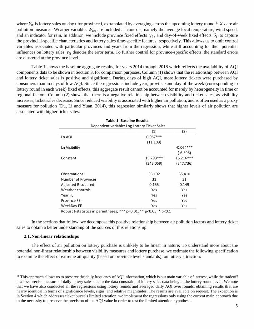
Table 1 shows the baseline aggregate results, for years 2014 through 2018 which reflects the availability of AQI
components data to be shown in Section 3, for comparison purposes. Column (1) shows that the relationship between AQI
and lottery ticket sales is positive and significant. During days of high AQI, more lottery tickets were purchased by
consumers than in days of low AQI. Since the regressions include year, province and day of the week (corresponding to
lottery round in each week) fixed effects, this aggregate result cannot be accounted for merely by heterogeneity in time or
regional factors. Column (2) shows that there is a negative relationship between visibility and ticket sales; as visibility
increases, ticket sales decrease. Since reduced visibility is associated with higher air pollution, and is often used as a proxy
measure for pollution (Du, Li and Yuan, 2014), this regression similarly shows that higher levels of air pollution are
associated with higher ticket sales.
Table 1. Baseline Results
Dependent variable: Log Lottery Ticket Sales
(1) (2)
Ln AQI 0.067***
(11.103)
Ln Visibility -0.064***
(-6.596)
Constant 15.793*** 16.216***
(343.059) (347.736)
Observations 56,102 55,410
Number of Provinces 31 31
Adjusted R-squared 0.155 0.149
Weather controls Yes Yes
Year FE Yes Yes
Province FE Yes Yes
WeekDay FE Yes Yes
Robust t-statistics in parentheses; *** p<0.01, ** p<0.05, * p<0.1
In the sections that follow, we decompose this positive relationship between air pollution factors and lottery ticket
sales to obtain a better understanding of the sources of this relationship.
2.1. Non-linear relationships
The effect of air pollution on lottery purchase is unlikely to be linear in nature. To understand more about the
potential non-linear relationship between visibility measures and lottery purchase, we estimate the following specification
to examine the effect of extreme air quality (based on province level standards), on lottery attraction:
11 This approach allows us to preserve the daily frequency of AQI information, which is our main variable of interest, while the tradeoff
is a less precise measure of daily lottery sales due to the data constraint of lottery sales data being at the lottery round level. We note
that we have also conducted all the regressions using lottery rounds and averaged daily AQI over rounds, obtaining results that are
nearly identical in terms of significance levels, signs, and relative magnitudes. The results are available on request. The exception is
in Section 4 which addresses ticket buyer’s limited attention, we implement the regressions only using the current main approach due
to the necessity to preserve the precision of the AQI value in order to test the limited attention hypothesis.
6
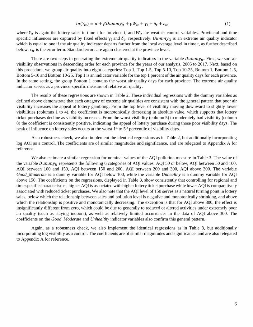
𝑙𝑛(𝑌𝑖𝑡) = 𝛼 + 𝛽𝐷𝑢𝑚𝑚𝑦𝑖𝑡 + ρ𝑊𝑖𝑡 + γ𝑖 + 𝛿𝑡 + 휀𝑖𝑡 (1)
where 𝑌𝑖𝑡 is again the lottery sales in time t for province i, and 𝑊𝑖𝑡 are weather control variables. Provincial and time
specific influences are captured by fixed effects γ𝑖 and 𝛿𝑡 , respectively. 𝐷𝑢𝑚𝑚𝑦𝑖𝑡 is an extreme air quality indicator
which is equal to one if the air quality indicator departs farther from the local average level in time t, as further described
below. 휀𝑖𝑡 is the error term. Standard errors are again clustered at the province level.
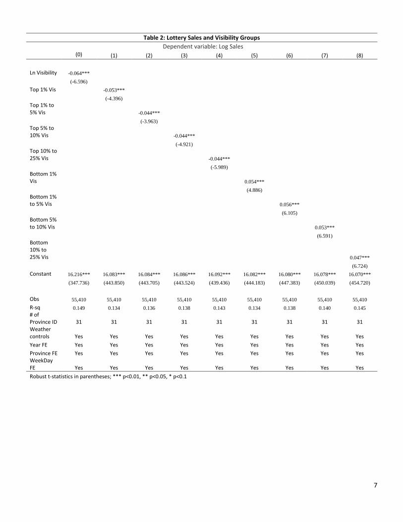
There are two steps in generating the extreme air quality indicators in the variable 𝐷𝑢𝑚𝑚𝑦𝑖𝑡. First, we sort air
visibility observations in descending order for each province for the years of our analysis, 2005 to 2017. Next, based on
this procedure, we group air quality into eight categories: Top 1, Top 1-5, Top 5-10, Top 10-25, Bottom 1, Bottom 1-5,
Bottom 5-10 and Bottom 10-25. Top 1 is an indicator variable for the top 1 percent of the air quality days for each province.
In the same setting, the group Bottom 1 contains the worst air quality days for each province. The extreme air quality
indicator serves as a province-specific measure of relative air quality.
The results of these regressions are shown in Table 2. These individual regressions with the dummy variables as
defined above demonstrate that each category of extreme air qualities are consistent with the general pattern that poor air
visibility increases the appeal of lottery gambling. From the top level of visibility moving downward to slightly lower
visibilities (columns 1 to 4), the coefficient is monotonically decreasing in absolute value, which supports that lottery
ticket purchases decline as visibility increases. From the worst visibility (column 5) to moderately bad visibility (column
8) the coefficient is consistently positive, indicating the appeal of lottery purchase during those poor visibility days. The
peak of influence on lottery sales occurs at the worst 1st to 5th percentile of visibility days.
As a robustness check, we also implement the identical regressions as in Table 2, but additionally incorporating
log AQI as a control. The coefficients are of similar magnitudes and significance, and are relegated to Appendix A for
reference.
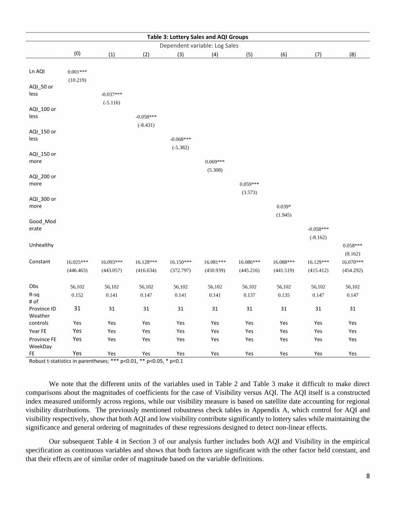
We also estimate a similar regression for nominal values of the AQI pollution measure in Table 3. The value of
the variable 𝐷𝑢𝑚𝑚𝑦𝑖𝑡 represents the following 6 categories of AQI values: AQI 50 or below, AQI between 50 and 100,
AQI between 100 and 150, AQI between 150 and 200, AQI between 200 and 300, AQI above 300. The variable
Good_Moderate is a dummy variable for AQI below 100, while the variable Unhealthy is a dummy variable for AQI
above 150. The coefficients on the regressions, displayed in Table 3, show consistently that controlling for regional and
time specific characteristics, higher AQI is associated with higher lottery ticket purchase while lower AQI is comparatively
associated with reduced ticket purchases. We also note that the AQI level of 150 serves as a natural turning point in lottery
sales, below which the relationship between sales and pollution level is negative and monotonically shrinking, and above
which the relationship is positive and monotonically decreasing. The exception is that for AQI above 300, the effect is
insignificantly different from zero, which could be due to generally to reduced or altered activities under extremely poor
air quality (such as staying indoors), as well as relatively limited occurrences in the data of AQI above 300. The
coefficients on the Good_Moderate and Unhealthy indicator variables also confirm this general pattern.
Again, as a robustness check, we also implement the identical regressions as in Table 3, but additionally
incorporating log visibility as a control. The coefficients are of similar magnitudes and significance, and are also relegated
to Appendix A for reference.
7
Table 2: Lottery Sales and Visibility Groups
Dependent variable: Log Sales
(0) (1) (2) (3) (4) (5) (6) (7) (8)
Ln Visibility -0.064***
(-6.596)
Top 1% Vis -0.053***
(-4.396)
Top 1% to 5% Vis
-0.044***
(-3.963) Top 5% to 10% Vis
-0.044***
(-4.921) Top 10% to 25% Vis
-0.044***
(-5.989) Bottom 1% Vis
0.054***
(4.886) Bottom 1% to 5% Vis
0.056***
(6.105) Bottom 5% to 10% Vis
0.053***
(6.591) Bottom 10% to 25% Vis
0.047***
(6.724)
Constant 16.216*** 16.083*** 16.084*** 16.086*** 16.092*** 16.082*** 16.080*** 16.078*** 16.070***
(347.736) (443.850) (443.705) (443.524) (439.436) (444.183) (447.383) (450.039) (454.720)
Obs 55,410 55,410 55,410 55,410 55,410 55,410 55,410 55,410 55,410
R-sq 0.149 0.134 0.136 0.138 0.143 0.134 0.138 0.140 0.145 # of Province ID 31 31 31 31 31 31 31 31 31 Weather controls Yes Yes Yes Yes Yes Yes Yes Yes Yes
Year FE Yes Yes Yes Yes Yes Yes Yes Yes Yes
Province FE Yes Yes Yes Yes Yes Yes Yes Yes Yes WeekDay FE Yes Yes Yes Yes Yes Yes Yes Yes Yes
Robust t-statistics in parentheses; *** p<0.01, ** p<0.05, * p<0.1
8
Table 3: Lottery Sales and AQI Groups
Dependent variable: Log Sales
(0) (1) (2) (3) (4) (5) (6) (7) (8)
Ln AQI 0.001***
(10.219)
AQI_50 or less
-0.037***
(-5.116)
AQI_100 or less
-0.058***
(-8.431) AQI_150 or less
-0.068***
(-5.382) AQI_150 or more
0.069***
(5.308) AQI_200 or more
0.059***
(3.573) AQI_300 or more
0.039*
(1.945) Good_Moderate
-0.058***
(-8.162) Unhealthy 0.058***
(8.162)
Constant 16.025*** 16.093*** 16.128*** 16.150*** 16.081*** 16.086*** 16.088*** 16.129*** 16.070***
(446.463) (443.057) (416.634) (372.797) (450.939) (445.216) (441.519) (415.412) (454.292)
Obs 56,102 56,102 56,102 56,102 56,102 56,102 56,102 56,102 56,102
R-sq 0.152 0.141 0.147 0.141 0.141 0.137 0.135 0.147 0.147 # of Province ID 31 31 31 31 31 31 31 31 31 Weather controls Yes Yes Yes Yes Yes Yes Yes Yes Yes
Year FE Yes Yes Yes Yes Yes Yes Yes Yes Yes
Province FE Yes Yes Yes Yes Yes Yes Yes Yes Yes WeekDay FE Yes Yes Yes Yes Yes Yes Yes Yes Yes
Robust t-statistics in parentheses; *** p<0.01, ** p<0.05, * p<0.1
We note that the different units of the variables used in Table 2 and Table 3 make it difficult to make direct
comparisons about the magnitudes of coefficients for the case of Visibility versus AQI. The AQI itself is a constructed
index measured uniformly across regions, while our visibility measure is based on satellite date accounting for regional
visibility distributions. The previously mentioned robustness check tables in Appendix A, which control for AQI and
visibility respectively, show that both AQI and low visibility contribute significantly to lottery sales while maintaining the
significance and general ordering of magnitudes of these regressions designed to detect non-linear effects.
Our subsequent Table 4 in Section 3 of our analysis further includes both AQI and Visibility in the empirical
specification as continuous variables and shows that both factors are significant with the other factor held constant, and
that their effects are of similar order of magnitude based on the variable definitions.

9
2.2 Effects across regions and seasons
It is widely perceived that northern China has substantially worse air quality than southern China, and these
perceptions are verified in the AQI data. Indeed, the differential heating policy in North and South leading to pollution
level differences has been previously utilized to identify the effect of air pollution on mortality (Almond, Chen, Greenstone
and Li, 2009; Chen, Ebenstein, Greenstone and Li, 2013). A natural question for our study of lottery gambling is whether
individuals in northern and southern China respond similarly to short-term variation in pollution with respect to lottery
ticket purchase decisions. Figure 1 shows the definition of northern and southern China, which is the commonly
acknowledged official definition.12
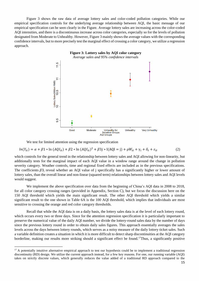
Figure 1: Map of Northern and Southern China
Subdividing the sample between northern and southern China using the standard definition depicted above, the
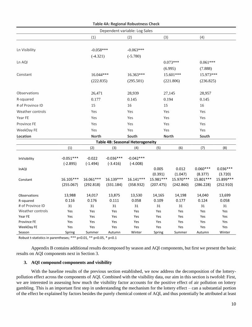
regression specifications in Table 4A show that the pollution-gambling relationship holds significantly across both North
and South, and that the effects are of similar magnitude, although of slightly stronger in magnitude in the North.
A further question is whether the pollution-lottery relationship is robust across seasons. Air pollution in China is
known to have a seasonal component. In particular, the average air pollution can often be higher in the winter due higher
energy usage via coal burning for heating systems. Table 4B shows the analogous regressions subdivided by the four
seasons in the year. The results show that summer is not the season that drives the relationship between pollution and
lottery gambling based on either the AQI measure or the visibility factor. Rather, autumn and winter are the predominant
seasons for both the visibility and AQI factors, while the effect is additionally present during spring under worsening
visibility conditions only.
Overall, the seasonality regressions confirm the conventional wisdom about the relative impacts of air pollution
by region and season, and show that the effect is regionally robust, while having greater concentration in the autumn and
winter seasons.
12 The red line shown in Figure 1 is also the dividing line above which publicly provided centralized heating is available, and below
which heating is not available, demarking the traditional division between north and south which corresponds to the Huai River.
10
Table 4A: Regional Robustness Check
Dependent variable: Log Sales
(1) (2) (3) (4)
Ln Visibility -0.058*** -0.063***
(-4.321) (-5.780) Ln AQI 0.073*** 0.061***
(6.995) (7.888)
Constant 16.044*** 16.363*** 15.601*** 15.973***
(222.835) (295.501) (221.806) (236.825)
Observations 26,471 28,939 27,145 28,957
R-squared 0.177 0.145 0.194 0.145
# of Province ID 15 16 15 16
Weather controls Yes Yes Yes Yes
Year FE Yes Yes Yes Yes
Province FE Yes Yes Yes Yes
WeekDay FE Yes Yes Yes Yes
Location North South North South
Table 4B: Seasonal Heterogeneity
(1) (2) (3) (4) (5) (6) (7) (8)
lnVisibility -0.051*** -0.022 -0.036*** -0.042***
(-2.895) (-1.494) (-3.416) (-4.008)
lnAQI 0.005 0.012 0.060*** 0.036***
(0.391) (1.047) (8.377) (3.720)
Constant 16.105*** 16.061*** 16.139*** 16.141*** 15.981*** 15.970*** 15.801*** 15.899***
(255.067) (292.818) (331.184) (358.932) (207.475) (242.860) (286.228) (252.910)
Observations 13,988 14,017 13,875 13,530 14,165 14,198 14,040 13,699
R-squared 0.116 0.176 0.111 0.058 0.109 0.177 0.124 0.058
# of Province ID 31 31 31 31 31 31 31 31
Weather controls Yes Yes Yes Yes Yes Yes Yes Yes
Year FE Yes Yes Yes Yes Yes Yes Yes Yes
Province FE Yes Yes Yes Yes Yes Yes Yes Yes
WeekDay FE Yes Yes Yes Yes Yes Yes Yes Yes
Season Spring Summer Autumn Winter Spring Summer Autumn Winter
Robust t-statistics in parentheses; *** p<0.01, ** p<0.05, * p<0.1
Appendix B contains additional results decomposed by season and AQI components, but first we present the basic
results on AQI components next in Section 3.
3. AQI compound components and visibility
With the baseline results of the previous section established, we now address the decomposition of the lottery-
pollution effect across the components of AQI. Combined with the visibility data, our aim in this section is twofold: First,
we are interested in assessing how much the visibility factor accounts for the positive effect of air pollution on lottery
gambling. This is an important first step in understanding the mechanism for the lottery effect – can a substantial portion
of the effect be explained by factors besides the purely chemical content of AQI, and thus potentially be attributed at least
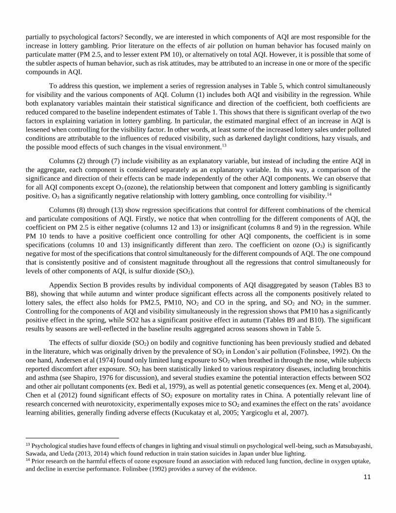
11
partially to psychological factors? Secondly, we are interested in which components of AQI are most responsible for the
increase in lottery gambling. Prior literature on the effects of air pollution on human behavior has focused mainly on
particulate matter (PM 2.5, and to lesser extent PM 10), or alternatively on total AQI. However, it is possible that some of
the subtler aspects of human behavior, such as risk attitudes, may be attributed to an increase in one or more of the specific
compounds in AQI.
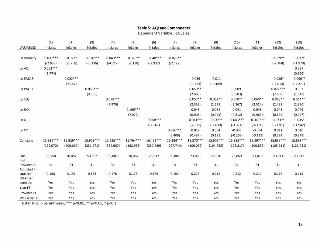
To address this question, we implement a series of regression analyses in Table 5, which control simultaneously
for visibility and the various components of AQI. Column (1) includes both AQI and visibility in the regression. While
both explanatory variables maintain their statistical significance and direction of the coefficient, both coefficients are
reduced compared to the baseline independent estimates of Table 1. This shows that there is significant overlap of the two
factors in explaining variation in lottery gambling. In particular, the estimated marginal effect of an increase in AQI is
lessened when controlling for the visibility factor. In other words, at least some of the increased lottery sales under polluted
conditions are attributable to the influences of reduced visibility, such as darkened daylight conditions, hazy visuals, and
the possible mood effects of such changes in the visual environment.13
Columns (2) through (7) include visibility as an explanatory variable, but instead of including the entire AQI in
the aggregate, each component is considered separately as an explanatory variable. In this way, a comparison of the
significance and direction of their effects can be made independently of the other AQI components. We can observe that
for all AQI components except O3 (ozone), the relationship between that component and lottery gambling is significantly
positive. O3 has a significantly negative relationship with lottery gambling, once controlling for visibility.14
Columns (8) through (13) show regression specifications that control for different combinations of the chemical
and particulate compositions of AQI. Firstly, we notice that when controlling for the different components of AQI, the
coefficient on PM 2.5 is either negative (columns 12 and 13) or insignificant (columns 8 and 9) in the regression. While
PM 10 tends to have a positive coefficient once controlling for other AQI components, the coefficient is in some
specifications (columns 10 and 13) insignificantly different than zero. The coefficient on ozone (O3) is significantly
negative for most of the specifications that control simultaneously for the different compounds of AQI. The one compound
that is consistently positive and of consistent magnitude throughout all the regressions that control simultaneously for
levels of other components of AQI, is sulfur dioxide (SO2).
Appendix Section B provides results by individual components of AQI disaggregated by season (Tables B3 to
B8), showing that while autumn and winter produce significant effects across all the components positively related to
lottery sales, the effect also holds for PM2.5, PM10, NO2 and CO in the spring, and SO2 and NO2 in the summer.
Controlling for the components of AQI and visibility simultaneously in the regression shows that PM10 has a significantly
positive effect in the spring, while SO2 has a significant positive effect in autumn (Tables B9 and B10). The significant
results by seasons are well-reflected in the baseline results aggregated across seasons shown in Table 5.
The effects of sulfur dioxide (SO2) on bodily and cognitive functioning has been previously studied and debated
in the literature, which was originally driven by the prevalence of SO2 in London’s air pollution (Folinsbee, 1992). On the
one hand, Andersen et al (1974) found only limited lung exposure to SO2 when breathed in through the nose, while subjects
reported discomfort after exposure. SO2 has been statistically linked to various respiratory diseases, including bronchitis
and asthma (see Shapiro, 1976 for discussion), and several studies examine the potential interaction effects between SO2
and other air pollutant components (ex. Bedi et al, 1979), as well as potential genetic consequences (ex. Meng et al, 2004).
Chen et al (2012) found significant effects of SO2 exposure on mortality rates in China. A potentially relevant line of
research concerned with neurotoxicity, experimentally exposes mice to SO2 and examines the effect on the rats’ avoidance
learning abilities, generally finding adverse effects (Kucukatay et al, 2005; Yargicoglu et al, 2007).
13 Psychological studies have found effects of changes in lighting and visual stimuli on psychological well-being, such as Matsubayashi,
Sawada, and Ueda (2013, 2014) which found reduction in train station suicides in Japan under blue lighting. 14 Prior research on the harmful effects of ozone exposure found an association with reduced lung function, decline in oxygen uptake,
and decline in exercise performance. Folinsbee (1992) provides a survey of the evidence.
12
The correlation between the chemical components of AQI in our data can be found in Section C of the Appendix.
The table shows that the daily measurements of these compounds are generally positively correlated, except for ozone (O3)
which tends to be negatively correlated with the other components. This can partially explain the persistent negative
coefficient found on the ozone variable in our regressions. PM 2.5 and PM 10 have the highest correlation with one another
(0.87), while the correlations between components (NO2 and CO) tends to be over 0.50. Sulfur dioxide (SO2) has a high
but relatively lower cross-correlation with the other components of AQI, which from a statistical standpoint, can explain
its significant ability to explain lottery purchase variation in comparison to the other compounds.
By implementing a more detailed analysis on the components of AQI in this section, and their relationship to
lottery gambling behavior, we can infer that other factors equal, sulfur dioxide significantly enhances lottery appeal while
ozone decreases it. Particulate matter (PM 2.5 and PM 10), while being the focus of several previous studies, is correlated
with, but appears to not be the underlying significant component through which pollution affects gambling.
13
Table 5: AQI and Components Dependent Variable: log Sales
(1) (2) (3) (4) (5) (6) (7) (8) (9) (10) (11) (12) (13)
VARIABLES lnSales lnSales lnSales lnSales lnSales lnSales lnSales lnSales lnSales lnSales lnSales lnSales lnSales
Ln Visibility -0.037*** -0.023* -0.036*** -0.040*** -0.026** -0.040*** -0.028** -0.039** -0.037*
(-2.858) (-1.758) (-3.336) (-4.717) (-2.138) (-2.937) (-2.122) (-2.168) (-1.979)
Ln AQI 0.052*** 0.037
(5.774) (0.599)
Ln PM2.5 0.052*** -0.059 -0.011 -0.086* -0.096**
(7.157) (-1.622) (-0.449) (-2.013) (-2.271)
Ln PM10 0.056*** 0.059** 0.009 0.072*** 0.053
(9.365) (2.483) (0.503) (2.806) (1.543)
Ln SO2 0.078*** 0.057** 0.062** 0.058** 0.060** 0.065** 0.064**
(7.970) (2.353) (2.525) (2.367) (2.524) (2.438) (2.390)
Ln NO2 0.106*** 0.048 0.051 0.041 0.046 0.048 0.049
(7.977) (0.908) (0.973) (0.812) (0.963) (0.894) (0.927)
Ln O3 -0.068*** -0.041*** -0.037** -0.043*** -0.040*** -0.033** -0.035*
(-7.167) (-2.871) (-2.639) (-3.311) (-4.160) (-2.091) (-1.942)
Ln CO 0.086*** 0.017 0.004 -0.008 -0.004 0.011 0.010
(5.408) (0.437) (0.121) (-0.263) (-0.139) (0.284) (0.249)
Constant 15.931*** 15.929*** 15.908*** 15.925*** 15.764*** 16.423*** 16.134*** 15.870*** 15.905*** 15.888*** 15.897*** 15.935*** 15.893***
(192.070) (209.666) (251.271) (384.667) (182.933) (250.249) (297.740) (106.059) (104.265) (108.817) (100.835) (105.911) (123.731)
Obs 55,158 50,887 50,882 50,887 50,887 23,612 50,887 23,869 23,870 23,869 23,870 23,611 23,547 # of ProvinceID 31 31 31 31 31 31 31 31 31 31 31 31 31 Adjusted R-squared 0.158 0.151 0.153 0.176 0.173 0.179 0.154 0.215 0.212 0.212 0.212 0.216 0.215 Weather controls Yes Yes Yes Yes Yes Yes Yes Yes Yes Yes Yes Yes Yes
Year FE Yes Yes Yes Yes Yes Yes Yes Yes Yes Yes Yes Yes Yes
Province FE Yes Yes Yes Yes Yes Yes Yes Yes Yes Yes Yes Yes Yes
WeekDay FE Yes Yes Yes Yes Yes Yes Yes Yes Yes Yes Yes Yes Yes
t-statistics in parentheses; *** p<0.01, ** p<0.05, * p<0.1
14
4. Attention and Color Categories
So far, in order to understand the mechanism behind air pollution’s effect on lottery gambling, we have
identified which official chemical components of air quality drive the effect and controlled for the visual factor
associated with pollution. If the pollution-lottery effect is not purely biological in nature as suggested by the visibility
data results, a natural subsequent question is whether individuals’ desire for lottery gambling is potentially
manipulable by the information and/or the presentation of information given the actual level of air pollution.
Since 2013, China’s government has publicly released information about regional air pollution conditions
through official AQI numbers, and additionally presented the public with color-coded categories to classify the
degree of pollution severity. The official AQI information were released and widely disseminated starting from
January 2013, as described in Barwick, Li, Lin and Zou (2019), which estimates the consumption and housing
response to pollution.15 Prior to this release date, AQI data existed nationwide, but was measured and reported by
different entities, such as local governments and U.S. embassies. The AQI information was not as easily accessible,
and importantly, the color-coded categorization of AQI levels was not in place at a national level prior to 2013.
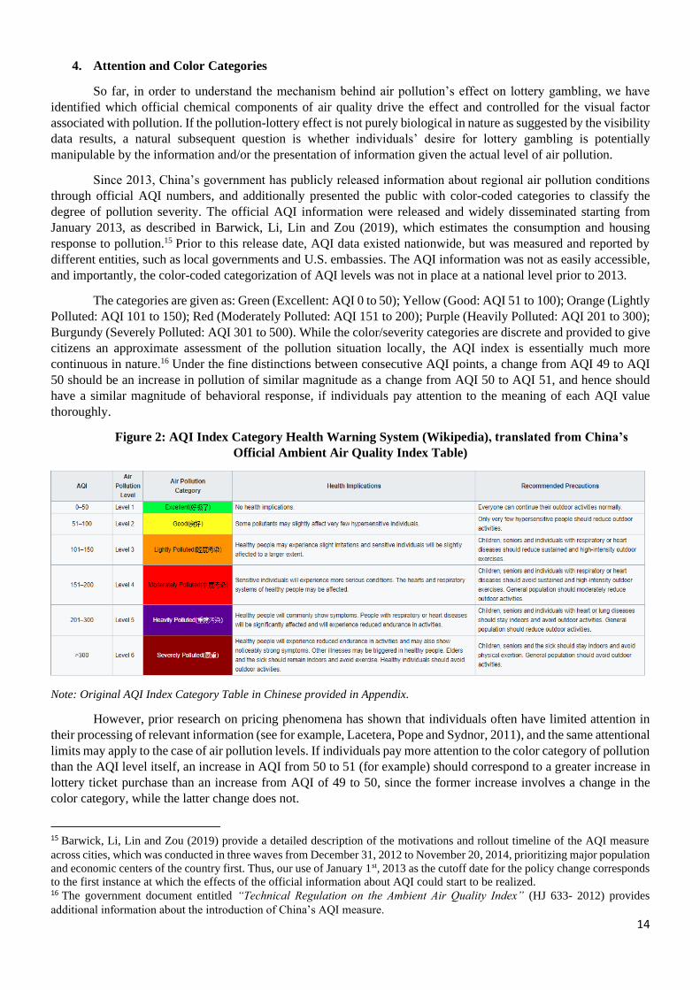
The categories are given as: Green (Excellent: AQI 0 to 50); Yellow (Good: AQI 51 to 100); Orange (Lightly
Polluted: AQI 101 to 150); Red (Moderately Polluted: AQI 151 to 200); Purple (Heavily Polluted: AQI 201 to 300);
Burgundy (Severely Polluted: AQI 301 to 500). While the color/severity categories are discrete and provided to give
citizens an approximate assessment of the pollution situation locally, the AQI index is essentially much more
continuous in nature.16 Under the fine distinctions between consecutive AQI points, a change from AQI 49 to AQI
50 should be an increase in pollution of similar magnitude as a change from AQI 50 to AQI 51, and hence should
have a similar magnitude of behavioral response, if individuals pay attention to the meaning of each AQI value
thoroughly.
Figure 2: AQI Index Category Health Warning System (Wikipedia), translated from China’s
Official Ambient Air Quality Index Table)
Note: Original AQI Index Category Table in Chinese provided in Appendix.
However, prior research on pricing phenomena has shown that individuals often have limited attention in
their processing of relevant information (see for example, Lacetera, Pope and Sydnor, 2011), and the same attentional
limits may apply to the case of air pollution levels. If individuals pay more attention to the color category of pollution
than the AQI level itself, an increase in AQI from 50 to 51 (for example) should correspond to a greater increase in
lottery ticket purchase than an increase from AQI of 49 to 50, since the former increase involves a change in the
color category, while the latter change does not.
15 Barwick, Li, Lin and Zou (2019) provide a detailed description of the motivations and rollout timeline of the AQI measure
across cities, which was conducted in three waves from December 31, 2012 to November 20, 2014, prioritizing major population
and economic centers of the country first. Thus, our use of January 1st, 2013 as the cutoff date for the policy change corresponds
to the first instance at which the effects of the official information about AQI could start to be realized. 16 The government document entitled “Technical Regulation on the Ambient Air Quality Index” (HJ 633- 2012) provides
additional information about the introduction of China’s AQI measure.
15
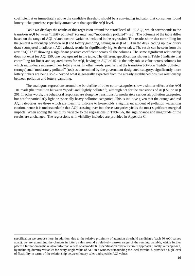
Figure 3 shows the raw data of average lottery sales and color-coded pollution categories. While our
empirical specification controls for the underlying average relationship between AQI, the basic message of our
empirical specification can be seen clearly in the Figure. Average lottery sales are increasing across the color-coded
AQI intensities, and there is a discontinuous increase across color categories, especially so for the levels of pollution
designated from Moderate to Unhealthy. However, Figure 3 mainly shows the average values with the corresponding
confidence intervals, but to more precisely test the marginal effect of crossing a color category, we utilize a regression
approach.
Figure 3: Lottery sales by AQI color category
Average sales and 95% confidence intervals
We test for limited attention using the regression specification
𝑙𝑛(𝑌𝑖𝑡) = 𝛼 + 𝛽1 ∗ ln(𝐴𝑄𝐼𝑖𝑡) + 𝛽2 ∗ ln(𝐴𝑄𝐼𝑖𝑡)2 + 𝛽3𝑗 ∗ I(AQI = j) + ρ𝑊𝑖𝑡 + γ𝑖 + 𝛿𝑡 + 휀𝑖𝑡 (2)
which controls for the general trend in the relationship between lottery sales and AQI allowing for non-linearity, but
additionally tests for the marginal impact of each AQI value in a window range around the change in pollution
severity category. Weather controls, time and regional fixed effects are included as in the previous specifications.
The coefficients 𝛽3j reveal whether an AQI value of j specifically has a significantly higher or lower amount of
lottery sales, than the overall linear and non-linear (squared term) relationships between lottery sales and AQI levels
would suggest.
We implement the above specification over data from the beginning of China’s AQI data in 2008 to 2018,
for all color category crossing ranges (provided in Appendix, Section C), but we focus the discussion here on the
150 AQI threshold which yields the main significant result. The other AQI threshold which yields a similar
significant result to the one shown in Table 6A is the 100 AQI threshold, which implies that individuals are most
sensitive to crossing the orange and red color category thresholds.
Recall that while the AQI data is on a daily basis, the lottery sales data is at the level of each lottery round,
which occurs every two or three days. Since for the attention regression specification it is particularly important to
preserve the numerical value of the daily AQI number, we divide the lottery-round sales data by the number of days
since the previous lottery round in order to obtain daily sales figures. This approach essentially averages the sales
levels across the days between lottery rounds, which serves as a noisy measure of the daily lottery ticket sales. Such
a variable definition creates a situation in which it is more difficult to detect sharp discontinuities at the AQI category
borderline, making our results more striking should a significant effect be found.17Thus, a significantly positive
17 A potentially intuitive alternative empirical approach to test our hypothesis could be to implement a traditional regression
discontinuity (RD) design. We utilize the current approach instead, for a few key reasons. For one, our running variable (AQI)
takes on strictly discrete values, which generally reduces the value added of a traditional RD approach compared to the
16
coefficient at or immediately above the candidate threshold should be a convincing indicator that consumers found
lottery ticket purchase especially attractive at that specific AQI level.
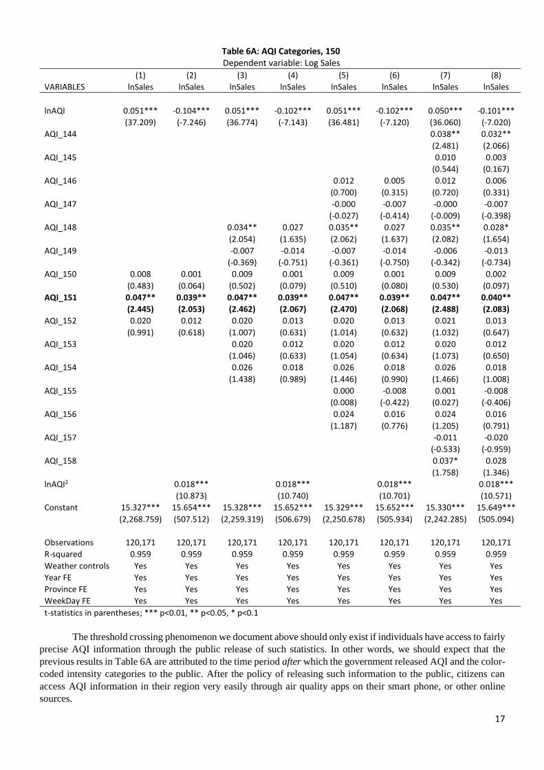
Table 6A displays the results of this regression around the cutoff level of 150 AQI, which corresponds to the
transition AQI between “lightly polluted” (orange) and “moderately polluted” (red). The columns of the table differ
based on the range of AQI-related control variables included in the regression. The results show that controlling for
the general relationship between AQI and lottery gambling, having an AQI of 151 in the days leading up to a lottery
draw (compared to adjacent AQI values), results in significantly higher ticket sales. The result can be seen from the
row “AQI 151” showing a significant positive coefficient across all the columns. The same significant relationship
does not exist for AQI 150, one row upward in the table. The different specifications shown in Table 5 indicate that
controlling for linear and squared terms for AQI, having an AQI of 151 is the only robust value across columns for
which individuals increased their lottery sales. In other words, precisely at the transition between “lightly polluted”
(orange) and “moderately polluted” (red) as determined by the government designated category, significantly more
lottery tickets are being sold - beyond what is generally expected from the already established positive relationship
between pollution and lottery gambling.
The analogous regressions around the borderline of other color categories show a similar effect at the AQI
101 mark (the transition between “good” and “lightly polluted”), although not for the transitions of AQI 51 or AQI
201. In other words, the behavioral responses are along the transitions for moderately serious air pollution categories,
but not for particularly light or especially heavy pollution categories. This is intuitive given that the orange and red
AQI categories are those which are meant to indicate to households a significant amount of pollution warranting
caution, hence it is understandable that AQI crossing over into these categories yields the most significant marginal
impacts. When adding the visibility variable to the regressions in Table 6A, the significance and magnitude of the
results are unchanged. The regressions with visibility included are provided in Appendix C.
specification we propose here. In addition, due to the relative proximity of attention threshold candidates (each 50 AQI values
apart), we are examining the changes in lottery sales around a relatively narrow range of the running variable, which further
places a limitation on the relative informativeness of a broader RD specification over our current approach. Finally, our approach,
by including dummy variables for every single value of AQI in a window surrounding the local threshold, provides a high level
of flexibility in terms of the relationship between lottery sales and specific AQI values.
17
Table 6A: AQI Categories, 150 Dependent variable: Log Sales
(1) (2) (3) (4) (5) (6) (7) (8)
VARIABLES lnSales lnSales lnSales lnSales lnSales lnSales lnSales lnSales
lnAQI 0.051*** -0.104*** 0.051*** -0.102*** 0.051*** -0.102*** 0.050*** -0.101***
(37.209) (-7.246) (36.774) (-7.143) (36.481) (-7.120) (36.060) (-7.020)
AQI_144 0.038** 0.032**
(2.481) (2.066)
AQI_145 0.010 0.003
(0.544) (0.167)
AQI_146 0.012 0.005 0.012 0.006
(0.700) (0.315) (0.720) (0.331)
AQI_147 -0.000 -0.007 -0.000 -0.007
(-0.027) (-0.414) (-0.009) (-0.398)
AQI_148 0.034** 0.027 0.035** 0.027 0.035** 0.028*
(2.054) (1.635) (2.062) (1.637) (2.082) (1.654)
AQI_149 -0.007 -0.014 -0.007 -0.014 -0.006 -0.013
(-0.369) (-0.751) (-0.361) (-0.750) (-0.342) (-0.734)
AQI_150 0.008 0.001 0.009 0.001 0.009 0.001 0.009 0.002
(0.483) (0.064) (0.502) (0.079) (0.510) (0.080) (0.530) (0.097)
AQI_151 0.047** 0.039** 0.047** 0.039** 0.047** 0.039** 0.047** 0.040**
(2.445) (2.053) (2.462) (2.067) (2.470) (2.068) (2.488) (2.083)
AQI_152 0.020 0.012 0.020 0.013 0.020 0.013 0.021 0.013
(0.991) (0.618) (1.007) (0.631) (1.014) (0.632) (1.032) (0.647)
AQI_153 0.020 0.012 0.020 0.012 0.020 0.012
(1.046) (0.633) (1.054) (0.634) (1.073) (0.650)
AQI_154 0.026 0.018 0.026 0.018 0.026 0.018
(1.438) (0.989) (1.446) (0.990) (1.466) (1.008)
AQI_155 0.000 -0.008 0.001 -0.008
(0.008) (-0.422) (0.027) (-0.406)
AQI_156 0.024 0.016 0.024 0.016
(1.187) (0.776) (1.205) (0.791)
AQI_157 -0.011 -0.020
(-0.533) (-0.959)
AQI_158 0.037* 0.028
(1.758) (1.346)
lnAQI2 0.018*** 0.018*** 0.018*** 0.018***
(10.873) (10.740) (10.701) (10.571)
Constant 15.327*** 15.654*** 15.328*** 15.652*** 15.329*** 15.652*** 15.330*** 15.649***
(2,268.759) (507.512) (2,259.319) (506.679) (2,250.678) (505.934) (2,242.285) (505.094)
Observations 120,171 120,171 120,171 120,171 120,171 120,171 120,171 120,171
R-squared 0.959 0.959 0.959 0.959 0.959 0.959 0.959 0.959
Weather controls Yes Yes Yes Yes Yes Yes Yes Yes
Year FE Yes Yes Yes Yes Yes Yes Yes Yes
Province FE Yes Yes Yes Yes Yes Yes Yes Yes
WeekDay FE Yes Yes Yes Yes Yes Yes Yes Yes
t-statistics in parentheses; *** p<0.01, ** p<0.05, * p<0.1
The threshold crossing phenomenon we document above should only exist if individuals have access to fairly
precise AQI information through the public release of such statistics. In other words, we should expect that the
previous results in Table 6A are attributed to the time period after which the government released AQI and the color-
coded intensity categories to the public. After the policy of releasing such information to the public, citizens can
access AQI information in their region very easily through air quality apps on their smart phone, or other online
sources.
18
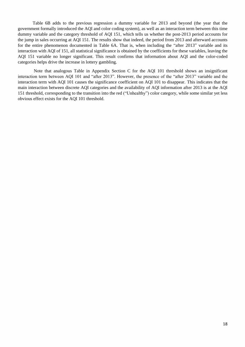
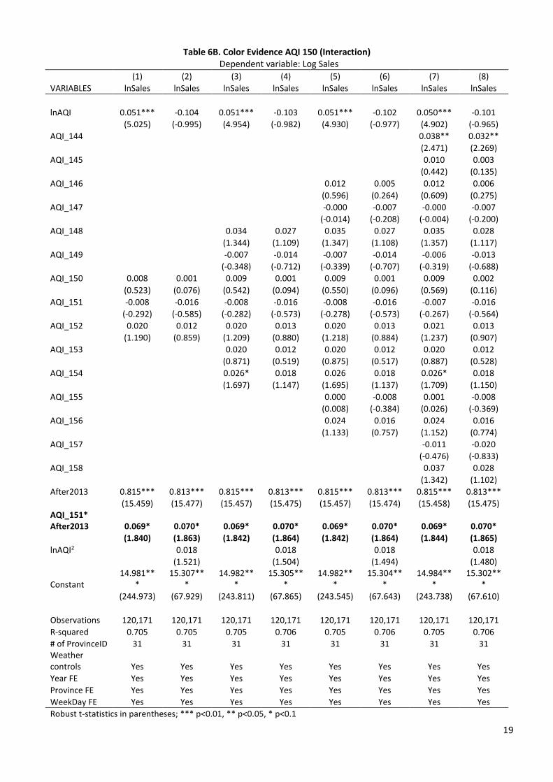
Table 6B adds to the previous regression a dummy variable for 2013 and beyond (the year that the
government formally introduced the AQI and color coding system), as well as an interaction term between this time
dummy variable and the category threshold of AQI 151, which tells us whether the post-2013 period accounts for
the jump in sales occurring at AQI 151. The results show that indeed, the period from 2013 and afterward accounts
for the entire phenomenon documented in Table 6A. That is, when including the “after 2013” variable and its
interaction with AQI of 151, all statistical significance is obtained by the coefficients for these variables, leaving the
AQI 151 variable no longer significant. This result confirms that information about AQI and the color-coded
categories helps drive the increase in lottery gambling.
Note that analogous Table in Appendix Section C for the AQI 101 threshold shows an insignificant
interaction term between AQI 101 and “after 2013”. However, the presence of the “after 2013” variable and the
interaction term with AQI 101 causes the significance coefficient on AQI 101 to disappear. This indicates that the
main interaction between discrete AQI categories and the availability of AQI information after 2013 is at the AQI
151 threshold, corresponding to the transition into the red (“Unhealthy”) color category, while some similar yet less
obvious effect exists for the AQI 101 threshold.
19
Table 6B. Color Evidence AQI 150 (Interaction) Dependent variable: Log Sales
(1) (2) (3) (4) (5) (6) (7) (8)
VARIABLES lnSales lnSales lnSales lnSales lnSales lnSales lnSales lnSales
lnAQI 0.051*** -0.104 0.051*** -0.103 0.051*** -0.102 0.050*** -0.101
(5.025) (-0.995) (4.954) (-0.982) (4.930) (-0.977) (4.902) (-0.965)
AQI_144 0.038** 0.032**
(2.471) (2.269)
AQI_145 0.010 0.003
(0.442) (0.135)
AQI_146 0.012 0.005 0.012 0.006
(0.596) (0.264) (0.609) (0.275)
AQI_147 -0.000 -0.007 -0.000 -0.007
(-0.014) (-0.208) (-0.004) (-0.200)
AQI_148 0.034 0.027 0.035 0.027 0.035 0.028
(1.344) (1.109) (1.347) (1.108) (1.357) (1.117)
AQI_149 -0.007 -0.014 -0.007 -0.014 -0.006 -0.013
(-0.348) (-0.712) (-0.339) (-0.707) (-0.319) (-0.688)
AQI_150 0.008 0.001 0.009 0.001 0.009 0.001 0.009 0.002
(0.523) (0.076) (0.542) (0.094) (0.550) (0.096) (0.569) (0.116)
AQI_151 -0.008 -0.016 -0.008 -0.016 -0.008 -0.016 -0.007 -0.016
(-0.292) (-0.585) (-0.282) (-0.573) (-0.278) (-0.573) (-0.267) (-0.564)
AQI_152 0.020 0.012 0.020 0.013 0.020 0.013 0.021 0.013
(1.190) (0.859) (1.209) (0.880) (1.218) (0.884) (1.237) (0.907)
AQI_153 0.020 0.012 0.020 0.012 0.020 0.012
(0.871) (0.519) (0.875) (0.517) (0.887) (0.528)
AQI_154 0.026* 0.018 0.026 0.018 0.026* 0.018
(1.697) (1.147) (1.695) (1.137) (1.709) (1.150)
AQI_155 0.000 -0.008 0.001 -0.008
(0.008) (-0.384) (0.026) (-0.369)
AQI_156 0.024 0.016 0.024 0.016
(1.133) (0.757) (1.152) (0.774)
AQI_157 -0.011 -0.020
(-0.476) (-0.833)
AQI_158 0.037 0.028
(1.342) (1.102)
After2013 0.815*** 0.813*** 0.815*** 0.813*** 0.815*** 0.813*** 0.815*** 0.813***
(15.459) (15.477) (15.457) (15.475) (15.457) (15.474) (15.458) (15.475) AQI_151* After2013 0.069* 0.070* 0.069* 0.070* 0.069* 0.070* 0.069* 0.070*
(1.840) (1.863) (1.842) (1.864) (1.842) (1.864) (1.844) (1.865)
lnAQI2 0.018 0.018 0.018 0.018
(1.521) (1.504) (1.494) (1.480)
Constant 14.981**
* 15.307**
* 14.982**
* 15.305**
* 14.982**
* 15.304**
* 14.984**
* 15.302**
*
(244.973) (67.929) (243.811) (67.865) (243.545) (67.643) (243.738) (67.610)
Observations 120,171 120,171 120,171 120,171 120,171 120,171 120,171 120,171
R-squared 0.705 0.705 0.705 0.706 0.705 0.706 0.705 0.706
# of ProvinceID 31 31 31 31 31 31 31 31 Weather controls Yes Yes Yes Yes Yes Yes Yes Yes
Year FE Yes Yes Yes Yes Yes Yes Yes Yes
Province FE Yes Yes Yes Yes Yes Yes Yes Yes
WeekDay FE Yes Yes Yes Yes Yes Yes Yes Yes
Robust t-statistics in parentheses; *** p<0.01, ** p<0.05, * p<0.1
20
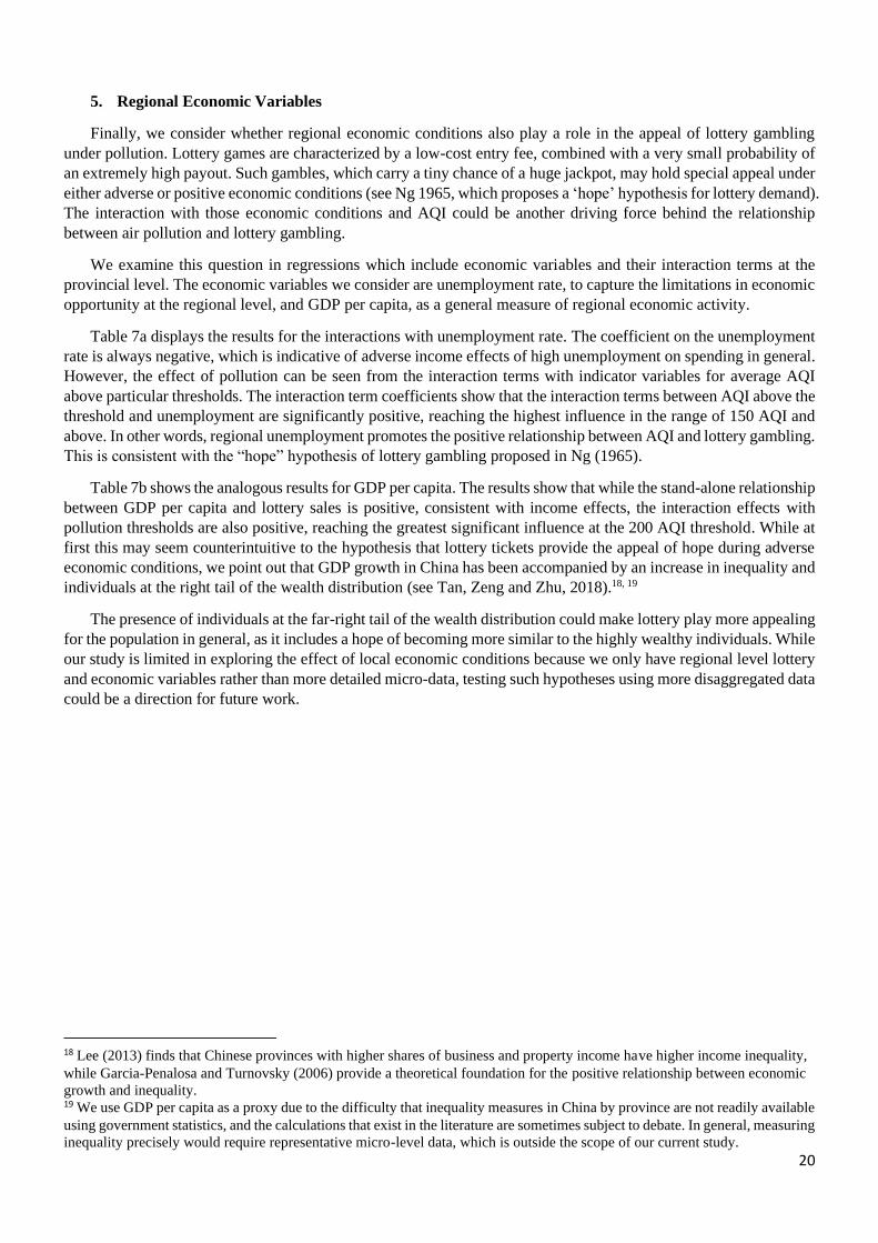
5. Regional Economic Variables
Finally, we consider whether regional economic conditions also play a role in the appeal of lottery gambling
under pollution. Lottery games are characterized by a low-cost entry fee, combined with a very small probability of
an extremely high payout. Such gambles, which carry a tiny chance of a huge jackpot, may hold special appeal under
either adverse or positive economic conditions (see Ng 1965, which proposes a ‘hope’ hypothesis for lottery demand).
The interaction with those economic conditions and AQI could be another driving force behind the relationship
between air pollution and lottery gambling.
We examine this question in regressions which include economic variables and their interaction terms at the
provincial level. The economic variables we consider are unemployment rate, to capture the limitations in economic
opportunity at the regional level, and GDP per capita, as a general measure of regional economic activity.
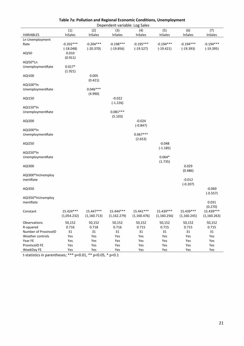
Table 7a displays the results for the interactions with unemployment rate. The coefficient on the unemployment
rate is always negative, which is indicative of adverse income effects of high unemployment on spending in general.
However, the effect of pollution can be seen from the interaction terms with indicator variables for average AQI
above particular thresholds. The interaction term coefficients show that the interaction terms between AQI above the
threshold and unemployment are significantly positive, reaching the highest influence in the range of 150 AQI and
above. In other words, regional unemployment promotes the positive relationship between AQI and lottery gambling.
This is consistent with the “hope” hypothesis of lottery gambling proposed in Ng (1965).
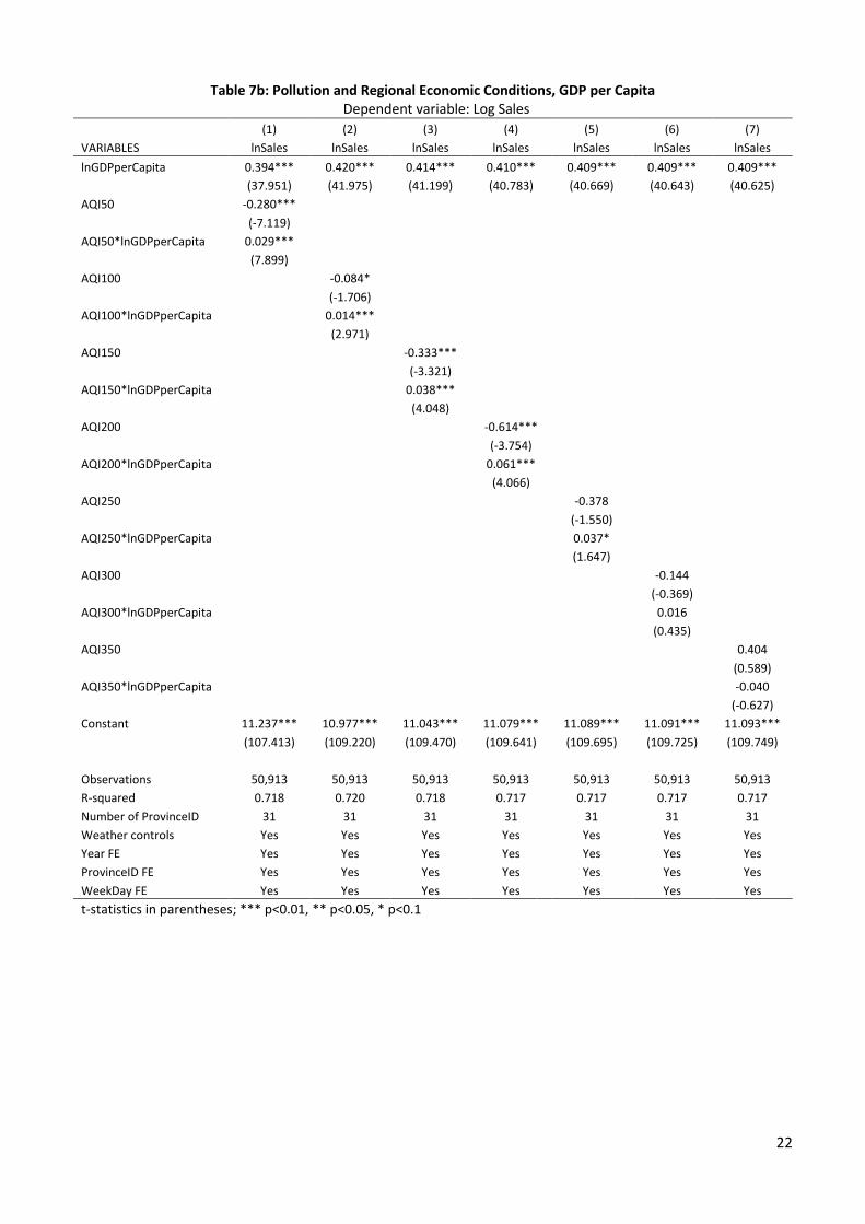
Table 7b shows the analogous results for GDP per capita. The results show that while the stand-alone relationship
between GDP per capita and lottery sales is positive, consistent with income effects, the interaction effects with
pollution thresholds are also positive, reaching the greatest significant influence at the 200 AQI threshold. While at
first this may seem counterintuitive to the hypothesis that lottery tickets provide the appeal of hope during adverse
economic conditions, we point out that GDP growth in China has been accompanied by an increase in inequality and
individuals at the right tail of the wealth distribution (see Tan, Zeng and Zhu, 2018).18, 19
The presence of individuals at the far-right tail of the wealth distribution could make lottery play more appealing
for the population in general, as it includes a hope of becoming more similar to the highly wealthy individuals. While
our study is limited in exploring the effect of local economic conditions because we only have regional level lottery
and economic variables rather than more detailed micro-data, testing such hypotheses using more disaggregated data
could be a direction for future work.
18 Lee (2013) finds that Chinese provinces with higher shares of business and property income have higher income inequality,
while Garcia-Penalosa and Turnovsky (2006) provide a theoretical foundation for the positive relationship between economic
growth and inequality. 19 We use GDP per capita as a proxy due to the difficulty that inequality measures in China by province are not readily available
using government statistics, and the calculations that exist in the literature are sometimes subject to debate. In general, measuring
inequality precisely would require representative micro-level data, which is outside the scope of our current study.
21
Table 7a: Pollution and Regional Economic Conditions, Unemployment Dependent variable: Log Sales
(1) (2) (3) (4) (5) (6) (7) VARIABLES lnSales lnSales lnSales lnSales lnSales lnSales lnSales
Ln Unemployment Rate -0.202*** -0.204*** -0.198*** -0.195*** -0.194*** -0.194*** -0.194***
(-18.048) (-20.370) (-19.856) (-19.527) (-19.421) (-19.393) (-19.395) AQI50 0.010
(0.911)
AQI50*Ln UnemploymentRate 0.017*
(1.921) AQI100 0.005
(0.421) AQI100*ln UnemploymentRate 0.046***
(4.990) AQI150 -0.022
(-1.226) AQI150*ln UnemploymentRate 0.081***
(5.103) AQI200 -0.024
(-0.847) AQI200*ln UnemploymentRate 0.067***
(2.653) AQI250 -0.048
(-1.185) AQI250*ln UnemploymentRate 0.064*
(1.735) AQI300 0.029
(0.486) AQI300*lnUnemploymentRate -0.012
(-0.207) AQI350 -0.069
(-0.557) AQI350*lnUnemploymentRate 0.031
(0.270) Constant 15.424*** 15.447*** 15.444*** 15.441*** 15.439*** 15.439*** 15.439***
(1,054.232) (1,160.713) (1,162.279) (1,160.476) (1,160.256) (1,160.245) (1,160.263)
Observations 50,152 50,152 50,152 50,152 50,152 50,152 50,152 R-squared 0.716 0.718 0.716 0.715 0.715 0.715 0.715 Number of ProvinceID 31 31 31 31 31 31 31 Weather controls Yes Yes Yes Yes Yes Yes Yes Year FE Yes Yes Yes Yes Yes Yes Yes ProvinceID FE Yes Yes Yes Yes Yes Yes Yes WeekDay FE Yes Yes Yes Yes Yes Yes Yes
t-statistics in parentheses; *** p<0.01, ** p<0.05, * p<0.1
22
Table 7b: Pollution and Regional Economic Conditions, GDP per Capita
Dependent variable: Log Sales
(1) (2) (3) (4) (5) (6) (7)
VARIABLES lnSales lnSales lnSales lnSales lnSales lnSales lnSales
lnGDPperCapita 0.394*** 0.420*** 0.414*** 0.410*** 0.409*** 0.409*** 0.409***
(37.951) (41.975) (41.199) (40.783) (40.669) (40.643) (40.625)
AQI50 -0.280***
(-7.119)
AQI50*lnGDPperCapita 0.029***
(7.899)
AQI100 -0.084*
(-1.706)
AQI100*lnGDPperCapita 0.014***
(2.971)
AQI150 -0.333***
(-3.321)
AQI150*lnGDPperCapita 0.038***
(4.048)
AQI200 -0.614***
(-3.754)
AQI200*lnGDPperCapita 0.061***
(4.066)
AQI250 -0.378
(-1.550)
AQI250*lnGDPperCapita 0.037*
(1.647)
AQI300 -0.144
(-0.369) AQI300*lnGDPperCapita 0.016
(0.435) AQI350 0.404
(0.589)
AQI350*lnGDPperCapita -0.040
(-0.627)
Constant 11.237*** 10.977*** 11.043*** 11.079*** 11.089*** 11.091*** 11.093***
(107.413) (109.220) (109.470) (109.641) (109.695) (109.725) (109.749)
Observations 50,913 50,913 50,913 50,913 50,913 50,913 50,913
R-squared 0.718 0.720 0.718 0.717 0.717 0.717 0.717
Number of ProvinceID 31 31 31 31 31 31 31
Weather controls Yes Yes Yes Yes Yes Yes Yes
Year FE Yes Yes Yes Yes Yes Yes Yes
ProvinceID FE Yes Yes Yes Yes Yes Yes Yes
WeekDay FE Yes Yes Yes Yes Yes Yes Yes
t-statistics in parentheses; *** p<0.01, ** p<0.05, * p<0.1
23
6. Conclusions
Poor air quality in some of the world’s rapidly expanding economies has inspired research on the influences of
air pollution on economic behavior. These influences can be roughly categorized as biologically driven, economically
driven and psychologically driven, perhaps roughly in order of inevitability. In this study, we examine some of the
potentially influential factors in each category with respect to lottery ticket purchase, one of the most popular forms
of gambling in China with low initial cost and high potential payoff.
We note that the significantly positive relationship between pollution and lottery gambling is directly counter to
the more general pollution avoidance effects on consumption found in Barwick, Li, Lin and Zou (2019). That is,
rather than avoiding purchases and purchase related activities due to the presence of pollution, consumers in fact
intentionally seek out the purchase of lottery tickets during high pollution periods. Given this arguably
counterintuitive positive effect in the broader context of pollution avoidance behavior, it is important to understand
what makes lottery tickets special in relation to local pollution levels.
Our analysis firstly indicates that the positive impact of air pollution on lottery gambling is in part biologically
driven, and in part psychologically driven, as evidenced by the persistence of statistically significant effects when
controlling for both AQI and visibility measures in the regressions. The robust chemical compound responsible for
the gambling effect is sulfur dioxide, which has been previously discussed as a main culprit in adverse health and
psychological effects of air pollution. This helps to pinpoint the main AQI component that could be attributed to
increased risk appetite and gambling tendencies, whereas prior studies on the effects of air quality on human behavior
have tended to focus primarily on particulate matter.
While the reduced visibility associated with air pollution is one psychological factor that plausibly leads to the
increased appeal of lottery tickets, attention to the reported quality of local air is another key factor. We test for the
attention factor induced by the Ministry of Environmental Protection’s color-coded categories, which are comprised
of discrete increments of 50 AQI points. While a purely biological effect of air pollution on gambling should
generally be insensitive to the exact AQI index value, paying close attention to the specific value of AQI rather than
the discrete color category should yield smooth responses of lottery ticket sales to changes in AQI values, regardless
of whether a color category is crossed.
However, we find that consumers discontinuously respond to AQI values that have just exactly crossed the
threshold into the next color-coded intensity level of pollution by buying disproportionately more lottery tickets,
reminiscent of the left digit bias found in Lacetera, Pope and Sydnor (2011). However, rather than using left digits
as the heuristic for pollution intensity, lottery buyers use the officially provided color category, particularly for the
transition in color from orange to red, which also corresponds to a particularly salient “alert” level. Such an effect is
driven entirely by the time period after the Ministry of Environmental Protection’s public release of the AQI statistics
and color categories, which were subsequently incorporated into cellular phone apps and websites, making such
information readily available to consumers. What this implies is that consumers are making a conscious decision to
buy lottery tickets after seeing that local AQI has crossed over into the red (“Unhealthy”) range. Alongside our
analyses on visibility versus chemical components, the color-coded evidence supports that the pollution effect on
gambling is significantly cognitive in nature.
While all of the above results help establish the importance of both biological and cognitive factors in the
pollution and gambling relationship, they reveal relatively little about the precise reasons for the appeal of lottery
tickets under polluted conditions. We then test whether the interaction between regional economic conditions and air
quality can provide any hint. Consistently with the ‘hope’ hypothesis regarding the motives for purchasing lottery
tickets (Ng, 1965), high regional unemployment rates enhance the pollution-gambling relationship. The consistency
with the hope hypothesis is that regions of scarcer earnings opportunities (ex. unemployment) may inspire more
activities which can give hope to residents. Higher gross domestic product per capita, typically associated in China
with increased inequality during our data time period, similarly promotes the necessity of hope among the less
fortunate comprising the great majority of the consumer base. Our empirical results are consistent with this line of
reasoning.
24
In summary, the relationship between air pollution and lottery gambling is due to several factors with regard to
poor air quality which work together to promote the appeal of lottery tickets. In addition to the biologically-driven
reaction towards the chemicals comprising air pollution, lower visibility, knowledge about AQI levels, heuristic
approaches to assessing the true air quality, and regional economic conditions all contribute significantly to this
appeal. The interaction between regional economic conditions and the pollution-gambling link suggests that high air
pollution could present a sense of bleakness in life that prompts the desire for hopeful gambles. Furthermore, at least
some of this effect is attributable to conscious decisions after having received detailed information and suggested
ways to understand air quality information.
25
References:
Almond, D., Chen, Y., Greenstone, M., and Li, H., “Winter Heating or Clean Air? Unintended Impacts of China’s Huai
River Policy”, American Economic Review, Papers and Proceedings, Vol. 99 (2009), No. 2, p. 184 – 190.
Andersen, I., Lundqvist, G.R., Jensen, P.L., and Proctor, D.F., “Human Response to Controlled Levels of Sulfur Dioxide”,
Archives of Environmental Health: An International Journal, Vol. 28 (1974), No. 1, p. 31 – 39.
Barwick, P.J., Li, S., Lin, L., and Zou, E., “From Fog to Smog: The Value of Pollution Information”, Working Paper,
May 2020.
Bedi, J.F., Folinsbee, L.J., Horvath, S.M., and Ebenstein, R.S., “Human Exposure to Sulfur Dioxide and Ozone: Absence
of a Synergistic Effect”, Archives of Environmental Health: An International Journal, Vol. 34 (1979), No. 4, p. 233 –
239.
Chang, T., Graff Zivin, J., Gross, T., and Neidell, M., “Particulate Pollution and the Productivity of Pear Packers”,
American Economic Journal: Economic Policy, Vol. 8 (2016), No. 3, p. 141 – 169.
Chang, T., Graff Zivin, J., and Neidell, M., The effect of pollution on office workers: Evidence form call centers in China,
American Economic Journal: Applied Economics, forthcoming
Chen, R., Huang, W., Wong, C., Wang, Z., Thach, T.Q., Chen, B., and Kan, H., “Short-term exposure to sulfur dioxide
and daily mortality in 17 Chinese cities: The China air pollution and health effects study (CAPES)”, Environmental
Research, Vol. 118 (2012), p. 101 – 106.
Chen, Y., Ebenstein, A., Greenstone, M., and Li, H., “Evidence on the Impact of Sustained Exposure to Air Pollution on
Life Expectancy from China’s Huai River Policy”, Proceedings of the National Academy of Sciences, Vol. 110 (2013),
No. 32, p. 12936 – 12941.
Chew, S., Huang, W., and Li, X., “Haze and decision making: A natural laboratory experiment”, Working paper, 2017.
Chew, S., Liu, H., and Salvo, A., “Air Pollution Raises Daily Lottery Demand in China”, Working paper, 2019.
Du, B., Li, Z., and Yuan, J., “Visibility has more to say about the pollution-income link”, Ecological Economics, Vol.
101 (2014) No. 5, p. 81 -98.
Folinsbee, L.J., “Human Health Effects of Air Pollution”, Environmental Health Perspectives, Vol. 100 (1992), p. 45 –
56.
Gao, F., Lien, J.W., Wang, Q., and Zheng, J. “Buy, hold or sell? Air quality and financial analyst reports”, Working
paper, 2019.
Garcia-Penalosa, C., and Turnovsky, S.J., “Growth and income inequality: a canonical model”, Economic Theory, Vol.
28 (2006), p. 25 – 49.
Graff Zivin, J., and Neidell, M., “The Impact of Pollution on Worker Productivity”, American Economic Review, Vol.
102 (2012), No. 7, p. 3652 – 3673.
He, J., Liu, H., and Salvo, A., “Severe air pollution and labor productivity: Evidence from industrial towns in China”,
American Economic Journal: Applied Economics, Vol. 11 (2019), No. 1, p. 173 – 201.
Humphreys, B.R. and Perez, L., “Network Externalities in Consumer Spending on Lottery Games: Evidence from Spain”,
Empirical Economics, Vol. 42 (2012), Issue 3, p. 929 – 945.
Humphreys, B.R. and Perez, L. “The ‘Who and Why’ of the Demand for Lottery: Empirical Highlights from the Seminal
Economic Literature”, Journal of Economic Surveys, Vol. 27 (2013), No. 5, p. 915 – 940.
Kucukatay, V., Savioglu, F., Hacioglu, G., Yargicoglu, P., and Agar, A., “Effect of sulfite on cognitive function in normal
and sulfite oxidase deficient rats”, Neurotoxicology and Teratology, Vol. 27 (2005), p. 47 – 54.
Lacetera, N., Pope, D.G., and Sydnor, J.R., “Heuristic Thinking and Limited Attention in the Car Market”, American
Economic Review, Vol. 102 (2012), No. 5, p. 2206 – 2236.
Lee, J., “A provincial perspective on income inequality in urban China and the role of property and business income”,
China Economic Review, Vol. 26 (2013), p. 140 – 150.
Lu, J.G., “Air pollution: A systematic review of its psychological, economic, and social effects”, Current Opinion in
Psychology, Vol. 32 (2020), p. 52 – 65.
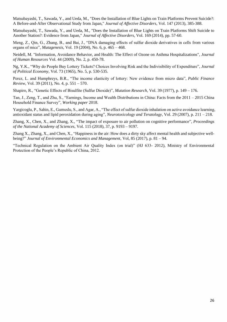
26
Matsubayashi, T., Sawada, Y., and Ueda, M., "Does the Installation of Blue Lights on Train Platforms Prevent Suicide?:
A Before-and-After Observational Study from Japan," Journal of Affective Disorders, Vol. 147 (2013), 385-388.
Matsubayashi, T., Sawada, Y., and Ueda, M., "Does the Installation of Blue Lights on Train Platforms Shift Suicide to
Another Station?: Evidence from Japan," Journal of Affective Disorders, Vol. 169 (2014), pp. 57-60.
Meng, Z., Qin, G., Zhang, B., and Bai, J., “DNA damaging effects of sulfur dioxide derivatives in cells from various
organs of mice”, Mutagenesis, Vol. 19 (2004), No. 6, p. 465 – 468.
Neidell, M. "Information, Avoidance Behavior, and Health: The Effect of Ozone on Asthma Hospitalizations", Journal
of Human Resources Vol. 44 (2009), No. 2, p. 450-78.
Ng, Y.K., “Why do People Buy Lottery Tickets? Choices Involving Risk and the Indivisibility of Expenditure”, Journal
of Political Economy, Vol. 73 (1965), No. 5, p. 530-535.
Perez, L. and Humphreys, B.R., “The income elasticity of lottery: New evidence from micro data”, Public Finance
Review, Vol. 39 (2011), No. 4, p. 551 – 570.
Shapiro, R., “Genetic Effects of Bisulfite (Sulfur Dioxide)”, Mutation Research, Vol. 39 (1977), p. 149 – 176.
Tan, J., Zeng, T., and Zhu, S., “Earnings, Income and Wealth Distributions in China: Facts from the 2011 – 2015 China
Household Finance Survey”, Working paper 2018.
Yargicoglu, P., Sahin, E., Gumuslu, S., and Agar, A., “The effect of sulfur dioxide inhalation on active avoidance learning,
antioxidant status and lipid peroxidation during aging”, Neurotoxicology and Teratology, Vol. 29 (2007), p. 211 – 218.
Zhang, X., Chen, X., and Zhang, X., “The impact of exposure to air pollution on cognitive performance”, Proceedings
of the National Academy of Sciences, Vol. 115 (2018), 37, p. 9193 – 9197.
Zhang X., Zhang, X., and Chen, X., “Happiness in the air: How does a dirty sky affect mental health and subjective well-
being?” Journal of Environmental Economics and Management, Vol, 85 (2017), p. 81 – 94.
“Technical Regulation on the Ambient Air Quality Index (on trial)” (HJ 633- 2012), Ministry of Environmental
Protection of the People’s Republic of China, 2012.

27
Appendix Section A: Summary Statistics and Robustness Checks with AQI and Visibility Measures
Table A1: Summary statistics
Variable Obs Mean Std. Dev. Min Max
Union Lotto Sales 56358 11000000.00 7087779.00 166072.00 89000000.00
Air Visibility 56777 9.78 4.29 0.15 18.60
Air Quality Index 56282 75.45 41.76 12.27 500.00
Pm 2.5 51796 45.01 32.12 4.10 471.28
Pm 10 51791 80.88 52.91 6.08 1067.61
So2 51796 19.93 17.96 1.94 270.06
No2 51796 30.47 15.07 3.93 176.22
O3 23870 57.09 24.68 2.20 173.57
Co 51796 1.01 1.07 0.20 124.30
Tables A2 and A3 show that the results of Tables 2 and 3 in Section 2.1 are robust to the inclusion of the AQI and
Visibility variables in the regressions, respectively.
Table A2: Lottery Sales and Visibility Groups (adding LnAQI)
Dependent variable: Log Sales
(1) (2) (3) (4) (5) (6) (7) (8)
Top 1% Vis -0.031**
(-2.522) Top 1% to 5% Vis -0.023*
(-1.961) Top 5% to 10% Vis -0.024**
(-2.503) Top 10% to 25% Vis -0.026***
(-3.158) Bottom 1% Vis 0.009
(0.657) Bottom 1% to 5% Vis 0.022**
(2.106) Bottom 5% to 10% Vis 0.024**
(2.675) Bottom 10% to 25% Vis 0.026***
(3.218) lnAQI 0.068*** 0.067*** 0.065*** 0.060*** 0.069*** 0.065*** 0.063*** 0.057***
(12.501) (11.440) (10.661) (9.312) (11.967) (10.564) (9.673) (8.294) Constant 15.779*** 15.786*** 15.796*** 15.822*** 15.778*** 15.791*** 15.803*** 15.822***
(370.025) (354.363) (343.342) (317.165) (360.450) (336.937) (324.752) (321.177) Observations 55,158 55,158 55,158 55,158 55,158 55,158 55,158 55,158 R-squared 0.154 0.155 0.155 0.157 0.154 0.155 0.155 0.157 Number of ProvinceID 31 31 31 31 31 31 31 31 Weather controls Yes Yes Yes Yes Yes Yes Yes Yes Year FE Yes Yes Yes Yes Yes Yes Yes Yes Province FE Yes Yes Yes Yes Yes Yes Yes Yes WeekDay FE Yes Yes Yes Yes Yes Yes Yes Yes
Robust t-statistics in parentheses, *** p<0.01, ** p<0.05, * p<0.1
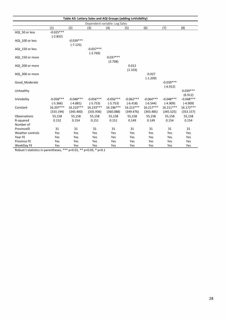
28
Table A3: Lottery Sales and AQI Groups (adding LnVisibility)
Dependent variable: Log Sales
(1) (2) (3) (4) (5) (6) (7) (8)
AQI_50 or less -0.025***
(-2.832) AQI_100 or less -0.039***
(-7.125) AQI_150 or less -0.037***
(-3.769) AQI_150 or more 0.037***
(3.708) AQI_200 or more 0.012
(1.103) AQI_300 or more -0.027
(-1.209) Good_Moderate -0.039***
(-6.912) Unhealthy 0.039***
(6.912) lnVisibility -0.058*** -0.048*** -0.056*** -0.056*** -0.062*** -0.064*** -0.048*** -0.048***
(-5.366) (-4.881) (-5.753) (-5.753) (-6.418) (-6.544) (-4.909) (-4.909) Constant 16.207*** 16.210*** 16.233*** 16.196*** 16.213*** 16.217*** 16.211*** 16.172***
(333.194) (345.400) (335.936) (360.088) (349.476) (343.485) (345.525) (353.157) Observations 55,158 55,158 55,158 55,158 55,158 55,158 55,158 55,158 R-squared 0.152 0.154 0.151 0.151 0.149 0.149 0.154 0.154 Number of ProvinceID 31 31 31 31 31 31 31 31 Weather controls Yes Yes Yes Yes Yes Yes Yes Yes Year FE Yes Yes Yes Yes Yes Yes Yes Yes Province FE Yes Yes Yes Yes Yes Yes Yes Yes WeekDay FE Yes Yes Yes Yes Yes Yes Yes Yes
Robust t-statistics in parentheses, *** p<0.01, ** p<0.05, * p<0.1
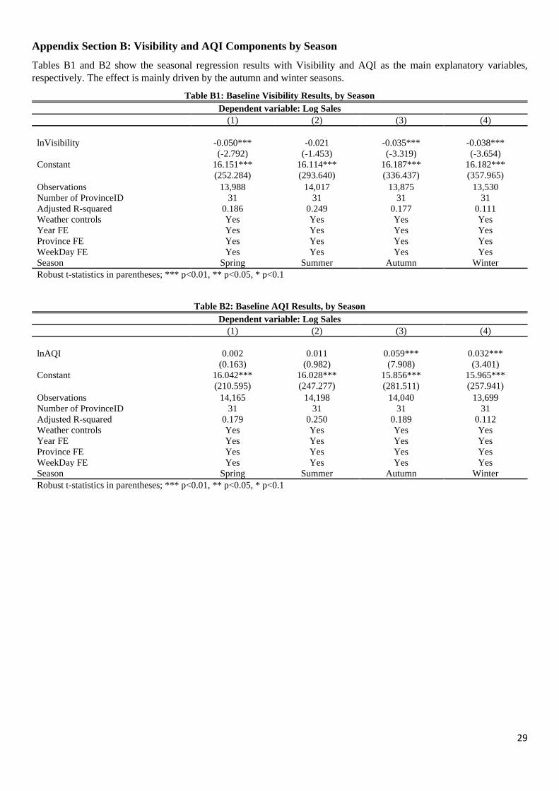
29
Appendix Section B: Visibility and AQI Components by Season
Tables B1 and B2 show the seasonal regression results with Visibility and AQI as the main explanatory variables,
respectively. The effect is mainly driven by the autumn and winter seasons.
Table B1: Baseline Visibility Results, by Season
Dependent variable: Log Sales
(1) (2) (3) (4)
lnVisibility -0.050*** -0.021 -0.035*** -0.038***
(-2.792) (-1.453) (-3.319) (-3.654)
Constant 16.151*** 16.114*** 16.187*** 16.182***
(252.284) (293.640) (336.437) (357.965) Observations 13,988 14,017 13,875 13,530
Number of ProvinceID 31 31 31 31
Adjusted R-squared 0.186 0.249 0.177 0.111
Weather controls Yes Yes Yes Yes
Year FE Yes Yes Yes Yes
Province FE Yes Yes Yes Yes
WeekDay FE Yes Yes Yes Yes
Season Spring Summer Autumn Winter
Robust t-statistics in parentheses; *** p<0.01, ** p<0.05, * p<0.1
Table B2: Baseline AQI Results, by Season
Dependent variable: Log Sales
(1) (2) (3) (4)
lnAQI 0.002 0.011 0.059*** 0.032***
(0.163) (0.982) (7.908) (3.401)
Constant 16.042*** 16.028*** 15.856*** 15.965***
(210.595) (247.277) (281.511) (257.941) Observations 14,165 14,198 14,040 13,699
Number of ProvinceID 31 31 31 31
Adjusted R-squared 0.179 0.250 0.189 0.112
Weather controls Yes Yes Yes Yes
Year FE Yes Yes Yes Yes
Province FE Yes Yes Yes Yes
WeekDay FE Yes Yes Yes Yes
Season Spring Summer Autumn Winter
Robust t-statistics in parentheses; *** p<0.01, ** p<0.05, * p<0.1

30
Tables B3 to B8 show the seasonal regressions for each AQI component separately. Individually, each AQI component with the
exception of O3 contributes positively to lottery sales in autumn and winter. Additionally SO2 and NO2 are significantly positive in
the summer, while particulate matter (PM10), NO2 and CO are significantly positive in the spring.
Table B3: Baseline PM2.5 Results, by Season
Dependent variable: Log Sales
(1) (2) (3) (4)
ln PM2.5 0.013 0.005 0.044*** 0.042***
(1.550) (0.452) (6.615) (7.862)
Constant 15.968*** 16.059*** 15.945*** 15.871***
(258.517) (251.456) (297.063) (436.001) Observations 12,833 13,919 14,103 10,941
Number of ProvinceID 31 31 31 31
Adjusted R-squared 0.166 0.259 0.189 0.075
Weather controls Yes Yes Yes Yes
Year FE Yes Yes Yes Yes
Province FE Yes Yes Yes Yes
WeekDay FE Yes Yes Yes Yes
Season Spring Summer Autumn Winter
Robust t-statistics in parentheses; *** p<0.01, ** p<0.05, * p<0.1
Table B4: Baseline PM10 Results, by Season
Dependent variable: Log Sales
(1) (2) (3) (4)
ln PM10 0.021*** 0.012 0.051*** 0.049***
(3.193) (1.113) (8.997) (6.285)
Constant 15.926*** 16.028*** 15.888*** 15.819***
(284.308) (248.710) (320.237) (396.292) Observations 12,833 13,919 14,100 10,939
Number of ProvinceID 31 31 31 31
Adjusted R-squared 0.168 0.259 0.189 0.076
Weather controls Yes Yes Yes Yes
Year FE Yes Yes Yes Yes
Province FE Yes Yes Yes Yes
WeekDay FE Yes Yes Yes Yes
Season Spring Summer Autumn Winter
Robust t-statistics in parentheses; *** p<0.01, ** p<0.05, * p<0.1
Table B5: Baseline SO2 Results, by Season
Dependent variable: Log Sales
(1) (2) (3) (4)
lnSo2 0.015 0.036** 0.085*** 0.069***
(1.123) (2.097) (7.089) (4.393)
Constant 15.973*** 15.977*** 15.840*** 15.813***
(278.642) (278.681) (286.735) (411.303) Observations 12,833 13,919 14,103 10,941
Number of ProvinceID 31 31 31 31
Adjusted R-squared 0.166 0.263 0.217 0.084
Weather controls Yes Yes Yes Yes
Year FE Yes Yes Yes Yes
Province FE Yes Yes Yes Yes
WeekDay FE Yes Yes Yes Yes
Season Spring Summer Autumn Winter
Robust t-statistics in parentheses; *** p<0.01, ** p<0.05, * p<0.1
31
Table B6: Baseline NO2 Results, by Season
Dependent variable: Log Sales
(1) (2) (3) (4)
lnNo2 0.034* 0.045* 0.084*** 0.090***
(1.997) (1.779) (6.352) (6.106)
Constant 15.901*** 15.930*** 15.815*** 15.734***
(209.424) (163.140) (221.360) (238.490) Observations 12,833 13,919 14,103 10,941
Number of ProvinceID 31 31 31 31
Adjusted R-squared 0.169 0.263 0.196 0.089
Weather controls Yes Yes Yes Yes
Year FE Yes Yes Yes Yes
Province FE Yes Yes Yes Yes
WeekDay FE Yes Yes Yes Yes
Season Spring Summer Autumn Winter
Robust t-statistics in parentheses; *** p<0.01, ** p<0.05, * p<0.1
Table B7: Baseline O3 Results, by Season
Dependent variable: Log Sales
(1) (2) (3) (4)
lno3 -0.037** -0.003 -0.036*** -0.098***
(-2.646) (-0.142) (-2.882) (-4.835)
Constant 16.173*** 16.093*** 16.252*** 16.410***
(204.381) (210.201) (331.026) (190.257) Observations 7,130 5,425 5,704 5,611
Number of ProvinceID 31 31 31 31
Adjusted R-squared 0.197 0.319 0.252 0.081
Weather controls Yes Yes Yes Yes
Year FE Yes Yes Yes Yes
Province FE Yes Yes Yes Yes
WeekDay FE Yes Yes Yes Yes
Season Spring Summer Autumn Winter
Robust t-statistics in parentheses; *** p<0.01, ** p<0.05, * p<0.1
Table B8: Baseline CO Results, by Season
Dependent variable: Log Sales
(1) (2) (3) (4)
lnCo 0.036** 0.021 0.066*** 0.055***
(2.500) (1.055) (4.420) (3.750)
Constant 16.018*** 16.080*** 16.113*** 16.030***
(391.598) (385.377) (381.061) (575.410) Observations 12,833 13,919 14,103 10,941
Number of ProvinceID 31 31 31 31
Adjusted R-squared 0.168 0.259 0.186 0.071
Weather controls Yes Yes Yes Yes
Year FE Yes Yes Yes Yes
Province FE Yes Yes Yes Yes
WeekDay FE Yes Yes Yes Yes
Season Spring Summer Autumn Winter
Robust t-statistics in parentheses; *** p<0.01, ** p<0.05, * p<0.1
Table B9 provides the seasonal regressions which include the decomposition of AQI components, omitting the aggregated AQI.
These specifications are useful for determining which components of AQI account positively for lottery sales by season. We can
observe that holding other AQI components constant, while PM10 is influential in the spring, SO2 is influential in the winter.
Table B10 additionally includes visibility as an explanatory variable, and finds results similar in significance and magnitude to
Table B9.
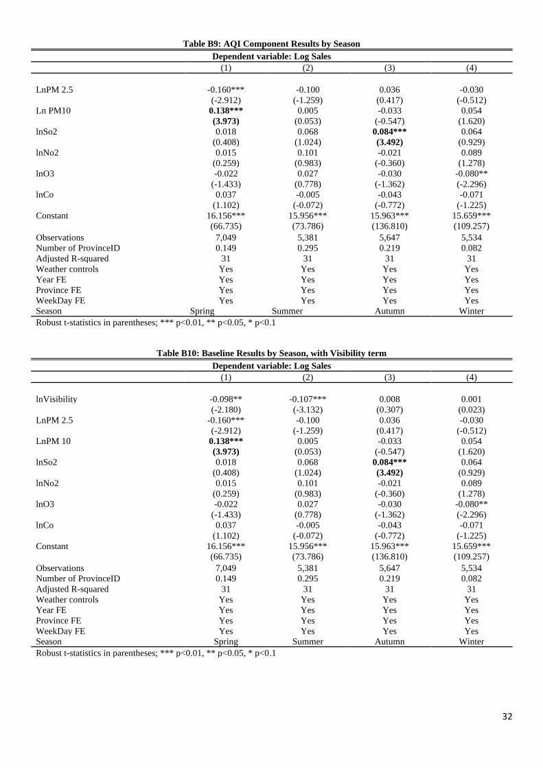
32
Table B9: AQI Component Results by Season
Dependent variable: Log Sales (1) (2) (3) (4)
LnPM 2.5 -0.160*** -0.100 0.036 -0.030
(-2.912) (-1.259) (0.417) (-0.512)
Ln PM10 0.138*** 0.005 -0.033 0.054
(3.973) (0.053) (-0.547) (1.620)
lnSo2 0.018 0.068 0.084*** 0.064
(0.408) (1.024) (3.492) (0.929)
lnNo2 0.015 0.101 -0.021 0.089
(0.259) (0.983) (-0.360) (1.278)
lnO3 -0.022 0.027 -0.030 -0.080**
(-1.433) (0.778) (-1.362) (-2.296)
lnCo 0.037 -0.005 -0.043 -0.071
(1.102) (-0.072) (-0.772) (-1.225)
Constant 16.156*** 15.956*** 15.963*** 15.659***
(66.735) (73.786) (136.810) (109.257) Observations 7,049 5,381 5,647 5,534
Number of ProvinceID 0.149 0.295 0.219 0.082
Adjusted R-squared 31 31 31 31
Weather controls Yes Yes Yes Yes
Year FE Yes Yes Yes Yes
Province FE Yes Yes Yes Yes
WeekDay FE Yes Yes Yes Yes
Season Spring Summer Autumn Winter
Robust t-statistics in parentheses; *** p<0.01, ** p<0.05, * p<0.1
Table B10: Baseline Results by Season, with Visibility term
Dependent variable: Log Sales (1) (2) (3) (4)
lnVisibility -0.098** -0.107*** 0.008 0.001
(-2.180) (-3.132) (0.307) (0.023)
LnPM 2.5 -0.160*** -0.100 0.036 -0.030
(-2.912) (-1.259) (0.417) (-0.512)
LnPM 10 0.138*** 0.005 -0.033 0.054
(3.973) (0.053) (-0.547) (1.620)
lnSo2 0.018 0.068 0.084*** 0.064
(0.408) (1.024) (3.492) (0.929)
lnNo2 0.015 0.101 -0.021 0.089
(0.259) (0.983) (-0.360) (1.278)
lnO3 -0.022 0.027 -0.030 -0.080**
(-1.433) (0.778) (-1.362) (-2.296)
lnCo 0.037 -0.005 -0.043 -0.071
(1.102) (-0.072) (-0.772) (-1.225)
Constant 16.156*** 15.956*** 15.963*** 15.659***
(66.735) (73.786) (136.810) (109.257) Observations 7,049 5,381 5,647 5,534
Number of ProvinceID 0.149 0.295 0.219 0.082
Adjusted R-squared 31 31 31 31
Weather controls Yes Yes Yes Yes
Year FE Yes Yes Yes Yes
Province FE Yes Yes Yes Yes
WeekDay FE Yes Yes Yes Yes
Season Spring Summer Autumn Winter
Robust t-statistics in parentheses; *** p<0.01, ** p<0.05, * p<0.1

33
Appendix Section C: Correlation between AQI Components
Table C1: Correlation matrix
Visibility AQI Pm2.5 Pm10 So2 No2 O3 Co
Visibility 1 AQI -0.381 1 Pm2.5 -0.476 0.950 1 Pm10 -0.268 0.930 0.865 1 So2 -0.174 0.508 0.503 0.493 1 No2 -0.426 0.704 0.733 0.624 0.527 1 O3 0.185 -0.071 -0.169 -0.074 -0.290 -0.295 1 Co -0.321 0.683 0.723 0.625 0.651 0.663 -0.356 1
Table C2: Pairwise correlation coefficients
Visibility AQI Pm2.5 Pm10 So2 No2 O3 Co
Visibility 1 AQI -0.370*** 1 Pm2.5 -0.485*** 0.949*** 1 Pm10 -0.259*** 0.929*** 0.842*** 1 So2 -0.158*** 0.504*** 0.510*** 0.468*** 1 No2 -0.433*** 0.685*** 0.724*** 0.584*** 0.479*** 1 O3 0.185*** -0.069*** -0.168*** -0.073*** -0.290*** -0.294*** 1 Co -0.165*** 0.335*** 0.376*** 0.278*** 0.284*** 0.319*** -0.356*** 1
Appendix Section D: Limited Attention, other AQI Categories and Placebo Tests
Figure 3 (Original): AQI Index Category Health Warning System (Original Chinese Table from the
Technical Regulation on the Ambient Air Quality Index)
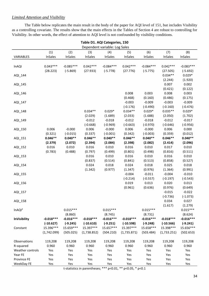
34
Limited Attention and Visibility
The Table below replicates the main result in the body of the paper for AQI level of 151, but includes Visibility
as a controlling covariate. The results show that the main effects in the Tables of Section 4 are robust to controlling for
Visibility. In other words, the effect of attention to AQI level is not confounded by visibility conditions.
Table D1. AQI Categories, 150 Dependent variable: Log Sales
(1) (2) (3) (4) (5) (6) (7) (8)
VARIABLES lnSales lnSales lnSales lnSales lnSales lnSales lnSales lnSales
lnAQI 0.043*** -0.085*** 0.042*** -0.084*** 0.042*** -0.084*** 0.042*** -0.083***
(28.223) (-5.869) (27.933) (-5.778) (27.776) (-5.775) (27.505) (-5.692)
AQI_144 0.034** 0.029*
(2.244) (1.920)
AQI_145 0.007 0.002
(0.421) (0.122)
AQI_146 0.008 0.003 0.008 0.003
(0.468) (0.160) (0.486) (0.175)
AQI_147 -0.003 -0.009 -0.003 -0.009
(-0.176) (-0.490) (-0.160) (-0.476)
AQI_148 0.034** 0.029* 0.034** 0.029* 0.035** 0.029*
(2.029) (1.689) (2.033) (1.688) (2.050) (1.702)
AQI_149 -0.012 -0.018 -0.012 -0.018 -0.012 -0.017
(-0.668) (-0.969) (-0.663) (-0.970) (-0.646) (-0.956)
AQI_150 0.006 -0.000 0.006 -0.000 0.006 -0.000 0.006 0.000
(0.321) (-0.015) (0.337) (-0.001) (0.342) (-0.003) (0.359) (0.012)
AQI_151 0.046** 0.040** 0.046** 0.040** 0.046** 0.040** 0.046** 0.040**
(2.379) (2.072) (2.394) (2.084) (2.398) (2.082) (2.414) (2.096)
AQI_152 0.016 0.010 0.016 0.010 0.016 0.010 0.017 0.010
(0.783) (0.488) (0.797) (0.499) (0.801) (0.498) (0.816) (0.511)
AQI_153 0.016 0.010 0.016 0.010 0.016 0.010
(0.837) (0.514) (0.841) (0.513) (0.858) (0.527)
AQI_154 0.024 0.018 0.024 0.018 0.025 0.018
(1.342) (0.977) (1.347) (0.976) (1.364) (0.991)
AQI_155 -0.004 -0.011 -0.004 -0.010
(-0.214) (-0.557) (-0.197) (-0.543)
AQI_156 0.019 0.013 0.020 0.013
(0.961) (0.636) (0.976) (0.649)
AQI_157 -0.015 -0.022
(-0.736) (-1.073)
AQI_158 0.034 0.027
(1.617) (1.279)
lnAQI2 0.015*** 0.015*** 0.015*** 0.015***
(8.860) (8.745) (8.731) (8.624)
lnVisibility -0.018*** -0.016*** -0.018*** -0.016*** -0.018*** -0.016*** -0.018*** -0.016***
(-10.627) (-9.245) (-10.610) (-9.251) (-10.598) (-9.248) (-10.566) (-9.241)
Constant 15.396*** 15.659*** 15.397*** 15.657*** 15.397*** 15.658*** 15.398*** 15.656***
(1,742.099) (505.025) (1,738.852) (504.210) (1,735.871) (503.484) (1,733.251) (502.653)
Observations 119,208 119,208 119,208 119,208 119,208 119,208 119,208 119,208
R-squared 0.960 0.960 0.960 0.960 0.960 0.960 0.960 0.960
Weather controls Yes Yes Yes Yes Yes Yes Yes Yes
Year FE Yes Yes Yes Yes Yes Yes Yes Yes
Province FE Yes Yes Yes Yes Yes Yes Yes Yes
WeekDay FE Yes Yes Yes Yes Yes Yes Yes Yes
t-statistics in parentheses; *** p<0.01, ** p<0.05, * p<0.1
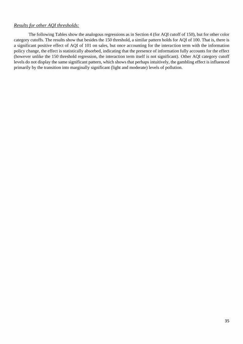
35
Results for other AQI thresholds:
The following Tables show the analogous regressions as in Section 4 (for AQI cutoff of 150), but for other color
category cutoffs. The results show that besides the 150 threshold, a similar pattern holds for AQI of 100. That is, there is
a significant positive effect of AQI of 101 on sales, but once accounting for the interaction term with the information
policy change, the effect is statistically absorbed, indicating that the presence of information fully accounts for the effect
(however unlike the 150 threshold regression, the interaction term itself is not significant). Other AQI category cutoff
levels do not display the same significant pattern, which shows that perhaps intuitively, the gambling effect is influenced
primarily by the transition into marginally significant (light and moderate) levels of pollution.
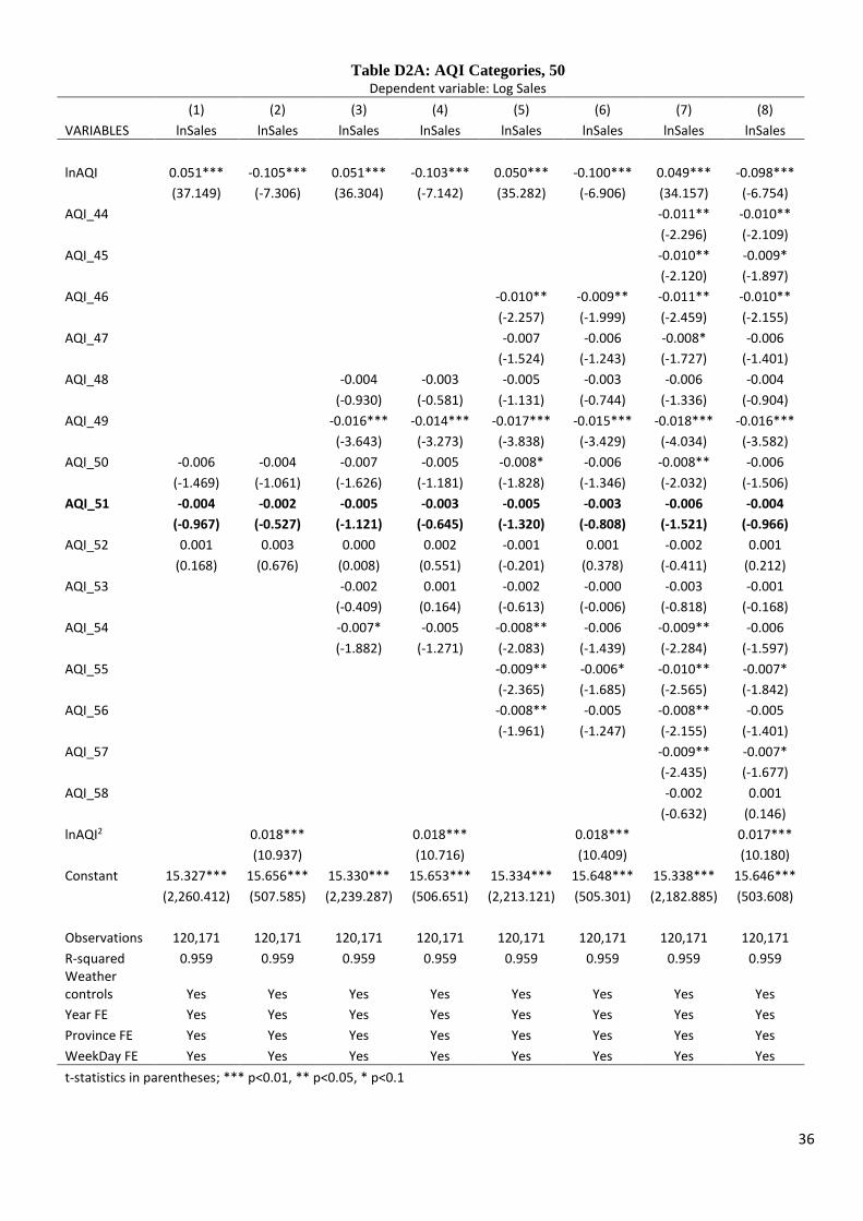
36
Table D2A: AQI Categories, 50 Dependent variable: Log Sales
(1) (2) (3) (4) (5) (6) (7) (8)
VARIABLES lnSales lnSales lnSales lnSales lnSales lnSales lnSales lnSales
lnAQI 0.051*** -0.105*** 0.051*** -0.103*** 0.050*** -0.100*** 0.049*** -0.098***
(37.149) (-7.306) (36.304) (-7.142) (35.282) (-6.906) (34.157) (-6.754)
AQI_44 -0.011** -0.010**
(-2.296) (-2.109)
AQI_45 -0.010** -0.009*
(-2.120) (-1.897)
AQI_46 -0.010** -0.009** -0.011** -0.010**
(-2.257) (-1.999) (-2.459) (-2.155)
AQI_47 -0.007 -0.006 -0.008* -0.006
(-1.524) (-1.243) (-1.727) (-1.401)
AQI_48 -0.004 -0.003 -0.005 -0.003 -0.006 -0.004
(-0.930) (-0.581) (-1.131) (-0.744) (-1.336) (-0.904)
AQI_49 -0.016*** -0.014*** -0.017*** -0.015*** -0.018*** -0.016***
(-3.643) (-3.273) (-3.838) (-3.429) (-4.034) (-3.582)
AQI_50 -0.006 -0.004 -0.007 -0.005 -0.008* -0.006 -0.008** -0.006
(-1.469) (-1.061) (-1.626) (-1.181) (-1.828) (-1.346) (-2.032) (-1.506)
AQI_51 -0.004 -0.002 -0.005 -0.003 -0.005 -0.003 -0.006 -0.004
(-0.967) (-0.527) (-1.121) (-0.645) (-1.320) (-0.808) (-1.521) (-0.966)
AQI_52 0.001 0.003 0.000 0.002 -0.001 0.001 -0.002 0.001
(0.168) (0.676) (0.008) (0.551) (-0.201) (0.378) (-0.411) (0.212)
AQI_53 -0.002 0.001 -0.002 -0.000 -0.003 -0.001
(-0.409) (0.164) (-0.613) (-0.006) (-0.818) (-0.168)
AQI_54 -0.007* -0.005 -0.008** -0.006 -0.009** -0.006
(-1.882) (-1.271) (-2.083) (-1.439) (-2.284) (-1.597)
AQI_55 -0.009** -0.006* -0.010** -0.007*
(-2.365) (-1.685) (-2.565) (-1.842)
AQI_56 -0.008** -0.005 -0.008** -0.005
(-1.961) (-1.247) (-2.155) (-1.401)
AQI_57 -0.009** -0.007*
(-2.435) (-1.677)
AQI_58 -0.002 0.001
(-0.632) (0.146)
lnAQI2 0.018*** 0.018*** 0.018*** 0.017***
(10.937) (10.716) (10.409) (10.180)
Constant 15.327*** 15.656*** 15.330*** 15.653*** 15.334*** 15.648*** 15.338*** 15.646***
(2,260.412) (507.585) (2,239.287) (506.651) (2,213.121) (505.301) (2,182.885) (503.608)
Observations 120,171 120,171 120,171 120,171 120,171 120,171 120,171 120,171
R-squared 0.959 0.959 0.959 0.959 0.959 0.959 0.959 0.959 Weather controls Yes Yes Yes Yes Yes Yes Yes Yes
Year FE Yes Yes Yes Yes Yes Yes Yes Yes
Province FE Yes Yes Yes Yes Yes Yes Yes Yes
WeekDay FE Yes Yes Yes Yes Yes Yes Yes Yes
t-statistics in parentheses; *** p<0.01, ** p<0.05, * p<0.1
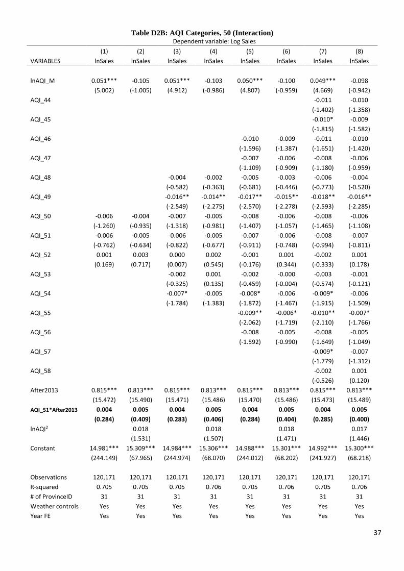
37
Table D2B: AQI Categories, 50 (Interaction) Dependent variable: Log Sales
(1) (2) (3) (4) (5) (6) (7) (8)
VARIABLES lnSales lnSales lnSales lnSales lnSales lnSales lnSales lnSales
lnAQI_M 0.051*** -0.105 0.051*** -0.103 0.050*** -0.100 0.049*** -0.098
(5.002) (-1.005) (4.912) (-0.986) (4.807) (-0.959) (4.669) (-0.942)
AQI_44 -0.011 -0.010
(-1.402) (-1.358)
AQI_45 -0.010* -0.009
(-1.815) (-1.582)
AQI_46 -0.010 -0.009 -0.011 -0.010
(-1.596) (-1.387) (-1.651) (-1.420)
AQI_47 -0.007 -0.006 -0.008 -0.006
(-1.109) (-0.909) (-1.180) (-0.959)
AQI_48 -0.004 -0.002 -0.005 -0.003 -0.006 -0.004
(-0.582) (-0.363) (-0.681) (-0.446) (-0.773) (-0.520)
AQI_49 -0.016** -0.014** -0.017** -0.015** -0.018** -0.016**
(-2.549) (-2.275) (-2.570) (-2.278) (-2.593) (-2.285)
AQI_50 -0.006 -0.004 -0.007 -0.005 -0.008 -0.006 -0.008 -0.006
(-1.260) (-0.935) (-1.318) (-0.981) (-1.407) (-1.057) (-1.465) (-1.108)
AQI_51 -0.006 -0.005 -0.006 -0.005 -0.007 -0.006 -0.008 -0.007
(-0.762) (-0.634) (-0.822) (-0.677) (-0.911) (-0.748) (-0.994) (-0.811)
AQI_52 0.001 0.003 0.000 0.002 -0.001 0.001 -0.002 0.001
(0.169) (0.717) (0.007) (0.545) (-0.176) (0.344) (-0.333) (0.178)
AQI_53 -0.002 0.001 -0.002 -0.000 -0.003 -0.001
(-0.325) (0.135) (-0.459) (-0.004) (-0.574) (-0.121)
AQI_54 -0.007* -0.005 -0.008* -0.006 -0.009* -0.006
(-1.784) (-1.383) (-1.872) (-1.467) (-1.915) (-1.509)
AQI_55 -0.009** -0.006* -0.010** -0.007*
(-2.062) (-1.719) (-2.110) (-1.766)
AQI_56 -0.008 -0.005 -0.008 -0.005
(-1.592) (-0.990) (-1.649) (-1.049)
AQI_57 -0.009* -0.007
(-1.779) (-1.312)
AQI_58 -0.002 0.001
(-0.526) (0.120)
After2013 0.815*** 0.813*** 0.815*** 0.813*** 0.815*** 0.813*** 0.815*** 0.813***
(15.472) (15.490) (15.471) (15.486) (15.470) (15.486) (15.473) (15.489)
AQI_51*After2013 0.004 0.005 0.004 0.005 0.004 0.005 0.004 0.005
(0.284) (0.409) (0.283) (0.406) (0.284) (0.404) (0.285) (0.400)
lnAQI2 0.018 0.018 0.018 0.017
(1.531) (1.507) (1.471) (1.446)
Constant 14.981*** 15.309*** 14.984*** 15.306*** 14.988*** 15.301*** 14.992*** 15.300***
(244.149) (67.965) (244.974) (68.070) (244.012) (68.202) (241.927) (68.218)
Observations 120,171 120,171 120,171 120,171 120,171 120,171 120,171 120,171
R-squared 0.705 0.705 0.705 0.706 0.705 0.706 0.705 0.706
# of ProvinceID 31 31 31 31 31 31 31 31
Weather controls Yes Yes Yes Yes Yes Yes Yes Yes
Year FE Yes Yes Yes Yes Yes Yes Yes Yes
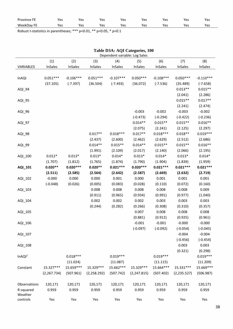
38
Province FE Yes Yes Yes Yes Yes Yes Yes Yes
WeekDay FE Yes Yes Yes Yes Yes Yes Yes Yes
Robust t-statistics in parentheses; *** p<0.01, ** p<0.05, * p<0.1
Table D3A: AQI Categories, 100 Dependent variable: Log Sales
(1) (2) (3) (4) (5) (6) (7) (8)
VARIABLES lnSales lnSales lnSales lnSales lnSales lnSales lnSales lnSales
lnAQI 0.051*** -0.106*** 0.051*** -0.107*** 0.050*** -0.108*** 0.050*** -0.110***
(37.105) (-7.397) (36.504) (-7.493) (36.072) (-7.536) (35.489) (-7.658)
AQI_94 0.013** 0.015**
(2.041) (2.286)
AQI_95 0.015** 0.017**
(2.241) (2.474)
AQI_96 -0.003 -0.002 -0.003 -0.002
(-0.473) (-0.294) (-0.422) (-0.236)
AQI_97 0.014** 0.015** 0.015** 0.016**
(2.075) (2.241) (2.125) (2.297)
AQI_98 0.017** 0.018*** 0.017** 0.018*** 0.018** 0.019***
(2.437) (2.600) (2.462) (2.629) (2.512) (2.686)
AQI_99 0.014** 0.015** 0.014** 0.015** 0.015** 0.016**
(1.991) (2.109) (2.017) (2.140) (2.066) (2.195)
AQI_100 0.012* 0.013* 0.013* 0.014* 0.013* 0.014* 0.013* 0.014*
(1.707) (1.812) (1.765) (1.874) (1.790) (1.904) (1.839) (1.959)
AQI_101 0.020** 0.020*** 0.020** 0.021*** 0.020*** 0.021*** 0.021*** 0.021***
(2.511) (2.585) (2.564) (2.642) (2.587) (2.669) (2.632) (2.719)
AQI_102 -0.000 0.000 0.000 0.001 0.000 0.001 0.001 0.001
(-0.048) (0.026) (0.005) (0.083) (0.028) (0.110) (0.072) (0.160)
AQI_103 0.008 0.008 0.008 0.008 0.008 0.009
(0.911) (0.965) (0.934) (0.991) (0.977) (1.040)
AQI_104 0.002 0.002 0.002 0.003 0.003 0.003
(0.244) (0.282) (0.266) (0.308) (0.310) (0.357)
AQI_105 0.007 0.008 0.008 0.008
(0.881) (0.912) (0.925) (0.961)
AQI_106 -0.001 -0.001 -0.000 -0.000
(-0.097) (-0.092) (-0.054) (-0.045)
AQI_107 -0.004 -0.004
(-0.456) (-0.454)
AQI_108 0.003 0.003
(0.321) (0.298)
lnAQI2 0.018*** 0.019*** 0.019*** 0.019***
(11.024) (11.087) (11.115) (11.209)
Constant 15.327*** 15.659*** 15.329*** 15.662*** 15.329*** 15.664*** 15.331*** 15.669***
(2,267.734) (507.961) (2,258.292) (507.742) (2,247.815) (507.402) (2,235.527) (506.987)
Observations 120,171 120,171 120,171 120,171 120,171 120,171 120,171 120,171
R-squared 0.959 0.959 0.959 0.959 0.959 0.959 0.959 0.959 Weather controls Yes Yes Yes Yes Yes Yes Yes Yes
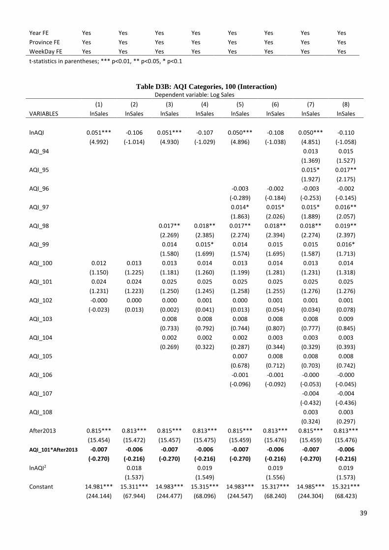
39
Year FE Yes Yes Yes Yes Yes Yes Yes Yes
Province FE Yes Yes Yes Yes Yes Yes Yes Yes
WeekDay FE Yes Yes Yes Yes Yes Yes Yes Yes
t-statistics in parentheses; *** p<0.01, ** p<0.05, * p<0.1
Table D3B: AQI Categories, 100 (Interaction) Dependent variable: Log Sales
(1) (2) (3) (4) (5) (6) (7) (8)
VARIABLES lnSales lnSales lnSales lnSales lnSales lnSales lnSales lnSales
lnAQI 0.051*** -0.106 0.051*** -0.107 0.050*** -0.108 0.050*** -0.110
(4.992) (-1.014) (4.930) (-1.029) (4.896) (-1.038) (4.851) (-1.058)
AQI_94 0.013 0.015
(1.369) (1.527)
AQI_95 0.015* 0.017**
(1.927) (2.175)
AQI_96 -0.003 -0.002 -0.003 -0.002
(-0.289) (-0.184) (-0.253) (-0.145)
AQI_97 0.014* 0.015* 0.015* 0.016**
(1.863) (2.026) (1.889) (2.057)
AQI_98 0.017** 0.018** 0.017** 0.018** 0.018** 0.019**
(2.269) (2.385) (2.274) (2.394) (2.274) (2.397)
AQI_99 0.014 0.015* 0.014 0.015 0.015 0.016*
(1.580) (1.699) (1.574) (1.695) (1.587) (1.713)
AQI_100 0.012 0.013 0.013 0.014 0.013 0.014 0.013 0.014
(1.150) (1.225) (1.181) (1.260) (1.199) (1.281) (1.231) (1.318)
AQI_101 0.024 0.024 0.025 0.025 0.025 0.025 0.025 0.025
(1.231) (1.223) (1.250) (1.245) (1.258) (1.255) (1.276) (1.276)
AQI_102 -0.000 0.000 0.000 0.001 0.000 0.001 0.001 0.001
(-0.023) (0.013) (0.002) (0.041) (0.013) (0.054) (0.034) (0.078)
AQI_103 0.008 0.008 0.008 0.008 0.008 0.009
(0.733) (0.792) (0.744) (0.807) (0.777) (0.845)
AQI_104 0.002 0.002 0.002 0.003 0.003 0.003
(0.269) (0.322) (0.287) (0.344) (0.329) (0.393)
AQI_105 0.007 0.008 0.008 0.008
(0.678) (0.712) (0.703) (0.742)
AQI_106 -0.001 -0.001 -0.000 -0.000
(-0.096) (-0.092) (-0.053) (-0.045)
AQI_107 -0.004 -0.004
(-0.432) (-0.436)
AQI_108 0.003 0.003
(0.324) (0.297)
After2013 0.815*** 0.813*** 0.815*** 0.813*** 0.815*** 0.813*** 0.815*** 0.813***
(15.454) (15.472) (15.457) (15.475) (15.459) (15.476) (15.459) (15.476)
AQI_101*After2013 -0.007 -0.006 -0.007 -0.006 -0.007 -0.006 -0.007 -0.006
(-0.270) (-0.216) (-0.270) (-0.216) (-0.270) (-0.216) (-0.270) (-0.216)
lnAQI2 0.018 0.019 0.019 0.019
(1.537) (1.549) (1.556) (1.573)
Constant 14.981*** 15.311*** 14.983*** 15.315*** 14.983*** 15.317*** 14.985*** 15.321***
(244.144) (67.944) (244.477) (68.096) (244.547) (68.240) (244.304) (68.423)
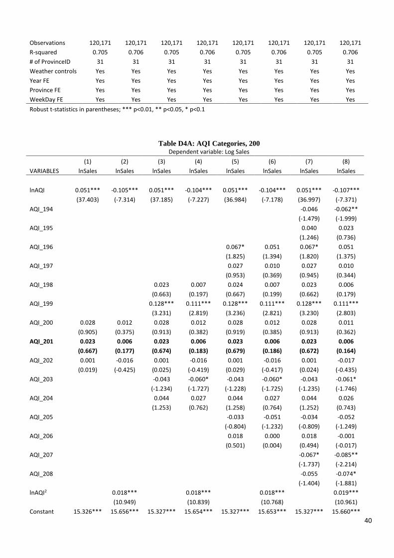
40
Observations 120,171 120,171 120,171 120,171 120,171 120,171 120,171 120,171
R-squared 0.705 0.706 0.705 0.706 0.705 0.706 0.705 0.706
# of ProvinceID 31 31 31 31 31 31 31 31
Weather controls Yes Yes Yes Yes Yes Yes Yes Yes
Year FE Yes Yes Yes Yes Yes Yes Yes Yes
Province FE Yes Yes Yes Yes Yes Yes Yes Yes
WeekDay FE Yes Yes Yes Yes Yes Yes Yes Yes
Robust t-statistics in parentheses; *** p<0.01, ** p<0.05, * p<0.1
Table D4A: AQI Categories, 200 Dependent variable: Log Sales
(1) (2) (3) (4) (5) (6) (7) (8)
VARIABLES lnSales lnSales lnSales lnSales lnSales lnSales lnSales lnSales
lnAQI 0.051*** -0.105*** 0.051*** -0.104*** 0.051*** -0.104*** 0.051*** -0.107***
(37.403) (-7.314) (37.185) (-7.227) (36.984) (-7.178) (36.997) (-7.371)
AQI_194 -0.046 -0.062**
(-1.479) (-1.999)
AQI_195 0.040 0.023
(1.246) (0.736)
AQI_196 0.067* 0.051 0.067* 0.051
(1.825) (1.394) (1.820) (1.375)
AQI_197 0.027 0.010 0.027 0.010
(0.953) (0.369) (0.945) (0.344)
AQI_198 0.023 0.007 0.024 0.007 0.023 0.006
(0.663) (0.197) (0.667) (0.199) (0.662) (0.179)
AQI_199 0.128*** 0.111*** 0.128*** 0.111*** 0.128*** 0.111***
(3.231) (2.819) (3.236) (2.821) (3.230) (2.803)
AQI_200 0.028 0.012 0.028 0.012 0.028 0.012 0.028 0.011
(0.905) (0.375) (0.913) (0.382) (0.919) (0.385) (0.913) (0.362)
AQI_201 0.023 0.006 0.023 0.006 0.023 0.006 0.023 0.006
(0.667) (0.177) (0.674) (0.183) (0.679) (0.186) (0.672) (0.164)
AQI_202 0.001 -0.016 0.001 -0.016 0.001 -0.016 0.001 -0.017
(0.019) (-0.425) (0.025) (-0.419) (0.029) (-0.417) (0.024) (-0.435)
AQI_203 -0.043 -0.060* -0.043 -0.060* -0.043 -0.061*
(-1.234) (-1.727) (-1.228) (-1.725) (-1.235) (-1.746)
AQI_204 0.044 0.027 0.044 0.027 0.044 0.026
(1.253) (0.762) (1.258) (0.764) (1.252) (0.743)
AQI_205 -0.033 -0.051 -0.034 -0.052
(-0.804) (-1.232) (-0.809) (-1.249)
AQI_206 0.018 0.000 0.018 -0.001
(0.501) (0.004) (0.494) (-0.017)
AQI_207 -0.067* -0.085**
(-1.737) (-2.214)
AQI_208 -0.055 -0.074*
(-1.404) (-1.881)
lnAQI2 0.018*** 0.018*** 0.018*** 0.019***
(10.949) (10.839) (10.768) (10.961)
Constant 15.326*** 15.656*** 15.327*** 15.654*** 15.327*** 15.653*** 15.327*** 15.660***
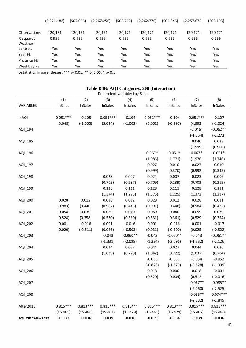
41
(2,271.182) (507.066) (2,267.256) (505.762) (2,262.776) (504.346) (2,257.672) (503.195)
Observations 120,171 120,171 120,171 120,171 120,171 120,171 120,171 120,171
R-squared 0.959 0.959 0.959 0.959 0.959 0.959 0.959 0.959 Weather controls Yes Yes Yes Yes Yes Yes Yes Yes
Year FE Yes Yes Yes Yes Yes Yes Yes Yes
Province FE Yes Yes Yes Yes Yes Yes Yes Yes
WeekDay FE Yes Yes Yes Yes Yes Yes Yes Yes
t-statistics in parentheses; *** p<0.01, ** p<0.05, * p<0.1
Table D4B: AQI Categories, 200 (Interaction) Dependent variable: Log Sales
(1) (2) (3) (4) (5) (6) (7) (8)
VARIABLES lnSales lnSales lnSales lnSales lnSales lnSales lnSales lnSales
lnAQI 0.051*** -0.105 0.051*** -0.104 0.051*** -0.104 0.051*** -0.107
(5.048) (-1.005) (5.024) (-1.002) (5.001) (-0.997) (4.993) (-1.024)
AQI_194 -0.046* -0.062**
(-1.754) (-2.273)
AQI_195 0.040 0.023
(1.599) (0.906)
AQI_196 0.067* 0.051* 0.067* 0.051*
(1.985) (1.771) (1.976) (1.746)
AQI_197 0.027 0.010 0.027 0.010
(0.999) (0.370) (0.992) (0.345)
AQI_198 0.023 0.007 0.024 0.007 0.023 0.006
(0.705) (0.237) (0.709) (0.239) (0.702) (0.215)
AQI_199 0.128 0.111 0.128 0.111 0.128 0.111
(1.374) (1.225) (1.375) (1.225) (1.372) (1.217)
AQI_200 0.028 0.012 0.028 0.012 0.028 0.012 0.028 0.011
(0.983) (0.440) (0.987) (0.445) (0.991) (0.448) (0.984) (0.422)
AQI_201 0.058 0.039 0.059 0.040 0.059 0.040 0.059 0.039
(0.528) (0.358) (0.530) (0.360) (0.531) (0.361) (0.529) (0.354)
AQI_202 0.001 -0.016 0.001 -0.016 0.001 -0.016 0.001 -0.017
(0.020) (-0.511) (0.026) (-0.503) (0.031) (-0.500) (0.025) (-0.522)
AQI_203 -0.043 -0.060** -0.043 -0.060** -0.043 -0.061**
(-1.331) (-2.098) (-1.324) (-2.096) (-1.332) (-2.126)
AQI_204 0.044 0.027 0.044 0.027 0.044 0.026
(1.039) (0.720) (1.042) (0.722) (1.037) (0.704)
AQI_205 -0.033 -0.051 -0.034 -0.052
(-0.823) (-1.379) (-0.828) (-1.399)
AQI_206 0.018 0.000 0.018 -0.001
(0.520) (0.004) (0.512) (-0.016)
AQI_207 -0.067** -0.085**
(-2.060) (-2.525)
AQI_208 -0.055** -0.074***
(-2.132) (-2.845)
After2013 0.815*** 0.813*** 0.815*** 0.813*** 0.815*** 0.813*** 0.815*** 0.813***
(15.461) (15.480) (15.461) (15.479) (15.461) (15.479) (15.462) (15.480)
AQI_201*After2013 -0.039 -0.036 -0.039 -0.036 -0.039 -0.036 -0.039 -0.036
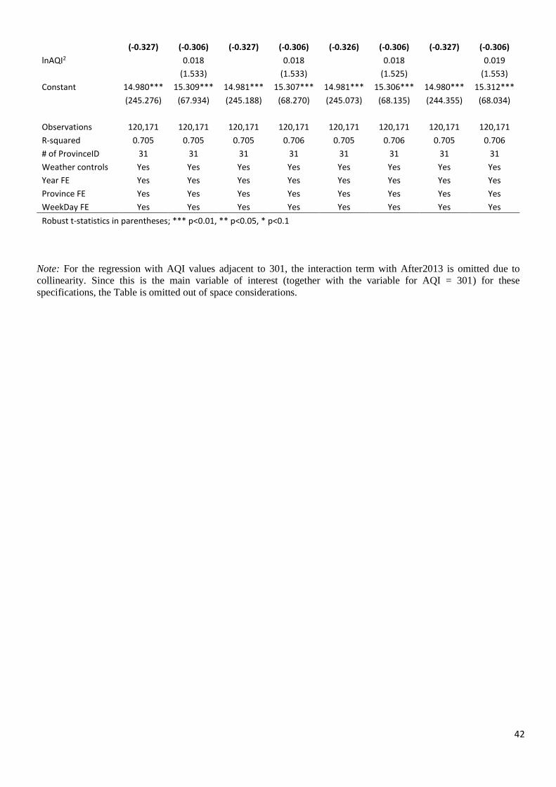
42
(-0.327) (-0.306) (-0.327) (-0.306) (-0.326) (-0.306) (-0.327) (-0.306)
lnAQI2 0.018 0.018 0.018 0.019
(1.533) (1.533) (1.525) (1.553)
Constant 14.980*** 15.309*** 14.981*** 15.307*** 14.981*** 15.306*** 14.980*** 15.312***
(245.276) (67.934) (245.188) (68.270) (245.073) (68.135) (244.355) (68.034)
Observations 120,171 120,171 120,171 120,171 120,171 120,171 120,171 120,171
R-squared 0.705 0.705 0.705 0.706 0.705 0.706 0.705 0.706
# of ProvinceID 31 31 31 31 31 31 31 31
Weather controls Yes Yes Yes Yes Yes Yes Yes Yes
Year FE Yes Yes Yes Yes Yes Yes Yes Yes
Province FE Yes Yes Yes Yes Yes Yes Yes Yes
WeekDay FE Yes Yes Yes Yes Yes Yes Yes Yes
Robust t-statistics in parentheses; *** p<0.01, ** p<0.05, * p<0.1
Note: For the regression with AQI values adjacent to 301, the interaction term with After2013 is omitted due to
collinearity. Since this is the main variable of interest (together with the variable for AQI = 301) for these
specifications, the Table is omitted out of space considerations.