NBER WORKING PAPER SERIES

LIVESTREAMING POLLUTION:A NEW FORM OF PUBLIC DISCLOSURE AND A CATALYST FOR CITIZEN ENGAGEMENT?

Emiliano Huet-VaughnNicholas MullerYen-Chia Hsu

Working Paper 24664http://www.nber.org/papers/w24664

NATIONAL BUREAU OF ECONOMIC RESEARCH1050 Massachusetts Avenue

Cambridge, MA 02138May 2018

The authors thank Karen Fisher-Vanden, Joel Landry, and seminar participants at the Penn State University Energy and Environmental Economics and Policy Seminar, as well as the Allegheny County Health Department for providing call records. The views expressed herein are those of the authors and do not necessarily reflect the views of the National Bureau of Economic Research.

NBER working papers are circulated for discussion and comment purposes. They have not been peer-reviewed or been subject to the review by the NBER Board of Directors that accompanies official NBER publications.

© 2018 by Emiliano Huet-Vaughn, Nicholas Muller, and Yen-Chia Hsu. All rights reserved. Short sections of text, not to exceed two paragraphs, may be quoted without explicit permission provided that full credit, including © notice, is given to the source.

Livestreaming Pollution: ¸˛A New Form of Public Disclosure and a Catalyst for Citizen Engagement?Emiliano Huet-Vaughn, Nicholas Muller, and Yen-Chia HsuNBER Working Paper No. 24664May 2018JEL No. D62,D91,Q52,Q53,Q55,Q58

ABSTRACT

Most environmental policy assumes the form of standards and enforcement. Scarce public budgets motivate the use of disclosure laws. This study explores a new form of pollution disclosure: real-time visual evidence of emissions provided on a free, public website. The paper tests whether the disclosure of visual evidence of emissions affects the nature and frequency of phone calls to the local air quality regulator. First, we test whether the presence of the camera affects the frequency of calls to the local air quality regulator about the facility monitored by the camera. Second, we test the relationship between the camera being active and the number of complaints about facilities other than the plant recorded by the camera. Our empirical results suggest that the camera did not affect the frequency of calls to the regulator about the monitored facility. However, the count of complaints pertaining to another prominent industrial polluter in the area, steel manufacturing plants, is positively associated with the camera being active. We propose two behavioral reasons for this finding: the prior knowledge hypothesis and affect heuristics. This study argues that visual evidence is a feasible approach to environmental oversight even during periods with diminished regulatory capacity.

Emiliano Huet-VaughnUniversity of California – Los Angeles 4284 School of Public AffairsLos Angeles, California 90095 ehuetvaughn@ucla.edu

Nicholas MullerDepartment of Engineering, and Public Policy Tepper School of BusinessCarnegie Mellon UniversityPosner 254C5000 Forbes AvenuePittsburgh, PA 15213and NBERnicholas.muller74@gmail.com

Yen-Chia HsuRobotics InstituteCarnegie Mellon University 5000 Forbes AvenuePittsburgh, PA 15213yenchiah@andrew.cmu.edu

2

Introduction.

Environmental policy in developed economies depends on effective monitoring and

enforcement. Monitoring ambient levels of pollution and direct mensuration of

emissions are expensive and therefore incomplete.1 A vast swath of the economy

remains unmonitored. Enforcement, which is often contentious, requires the

deployment of scarce public resources and is, therefore, imperfect. Recent

developments in the federal political environment suggest even more limited federal

enforcement (New York Times, 2017).

The dearth of pollution monitors and incomplete enforcement motivates public

disclosure as a means to affect change among polluting firms (Tietenberg, 1998). Direct

information on pollution provided to concerned citizens may enhance public pressure

on regulatory agencies to enforce existing rules and laws. Traditional approaches to

public disclosure in the environmental realm manifest as legal requirements for firms to

reveal, or list, their emissions (Graham, 2002). Prominent examples of disclosure laws

include the Toxic Release Inventory (TRI), and the Greenhouse Gas Reporting Program

(GHGRP), (40 CFR Part 98).

1 The current network of ambient air pollution monitors in the United States (see https://www.epa.gov/outdoor-air-quality-data) is sparsely distributed. Monitoring sites are typically chosen to maximize the likelihood of detecting a violation. Hence, the monitors are clustered in densely populated locations. Further, the Continuous Emissions Monitoring System (CEMS), an example of a system of emissions monitors, only tracks discharges of nitrogen oxides (NOx) and sulfur dioxide (SO2) at certain point sources.

3

This study focuses on a new means to provide the public with information on emissions

and ambient pollution: visual evidence of emissions captured by camera, and broadcast

on a free, public website. Essentially, livestreaming images of emissions is a means of

disclosing risk to the public. In contrast to perhaps more conventional means (such as

periodically reporting pollution levels or announcing risks to certain population

groups) broadcasting live imagery of emissions provides a contemporaneous view of

the threat from pollution in a more graphic, tangible, and visceral manner. Previous

research suggests that people react to risk messaging in two general ways: systematic,

or cognitive, responses and emotional responses (Lowenstein and Mather, 1990;

Lowenstein et al., 2001; Slovic et al., 2002; Dillard and Anderson, 2004; Hastings, Stead,

and Webb, 2004). Providing quantitative risk estimates - like direct measurements of

pollution data - clearly speaks to cognitive message processing. The camera targets

emotional reactions – anger or fear - that may trigger acute responses such as picking

up the phone and calling the local air quality regulator (Averbeck, Jones, and

Robertson, 2011).

Undergirding our analysis is the argument that visual disclosure may present a new set

of tools for regulators, environmental advocates, and concerned communities to affect

behavior of firms that manage to circumvent traditional regulatory frameworks.

Recognizing the potential for visual evidence as an important complement to customary

monitoring and enforcement, Giles (2013) notes that:

“[W]e are not far from the day when the public will have access to pollution monitoring tools. Communities with monitoring data will encourage better

4

performance by industries they host…These changes, driven by new technologies, will encourage more direct industry and community engagement, and reduce the need for

government action.”

In addition to its comprehensivity, particularly attractive is the cost-effectiveness of this

approach. Any demonstrable reduction in pollution attained through this approach

would come at very low opportunity cost, relative to more traditional approaches that

require significant allocations of physical and financial capital as well as labor

resources.2

1.1 Empirical Context

The analysis focuses on a now shuttered coke plant located just west of Pittsburgh,

Pennsylvania on Neville Island in the Ohio River: the Shenango Coke Works, or the

“mill”. Coke is purified coal; it is a nearly pure carbon substance produced by baking

coal to remove impurities. This site has repeatedly violated air pollution standards.3

The mill has received considerable attention in the local media and in nearby

communities (Pittsburgh Post-Gazette, 2015a).4 A robotic camera was installed to track

2 Over the past twenty years, there were over 19,000 inspections performed by the United States Environmental Protection Agency (USEPA), per year. Of these, about 1,000 to 3,000 were related to the Clean Air Act (CAA), (Shimshak, 2014). The USEPA’s Office of Enforcement and Compliance Assurance has an annual budget in the range of $600 million (Shimshak, 2014). 3 Recent examples of such violations include: Allegheny County (home to the plant) fined DTE Energy (the corporate owner of the plant) in late 2013. In the spring of 2014, the operator of the plant reached a settlement with the Allegheny County Health Department. The agreement contains specific changes to operations designed to reduce emissions, investments in pollution control technology, and fines related to earlier violations (Pittsburgh Tribune Review, 2014). Previously, in 2012, DTE reached a consent decree involving a $1.75 million penalty (Pittsburgh Post-Gazette, 2015b). 4 In particular, violations occurred in: 1980, 1993, 2000, 2005, 2012, and 2014.

5

visible emissions from the plant (Shenango Channel, 2015; Pittsburgh Post-Gazette,

2015b). The Shenango Channel first went live on November 15th, 2014, providing visual

smoke imagery online for most of the next three weeks until stopping the broadcast on

December 5th, 2014. Then, again, on January 22nd, 2015 the livestream began anew and

continued to broadcast for the duration of 2015. The imagery captured by the camera is

posted on a website devoted to providing visual evidence of emissions from the mill

(Shenango Channel, 2015). The device also generates quantitative estimates of the

opacity of emissions from the facility every five minutes. Emissions density is

quantified through pixel counts. Thus, in addition to the raw visual imagery posted

online, the camera provides a numerically based approach to real-time measurement of

emissions that is both more reliable than ad hoc observations made by members of

affected communities, and distinct from mensuration performed by regulators.

The empirical analysis begins with a test of whether there is an association between the

quantitative smoke readings produced by the camera’s algorithm and actual pollution

observations gathered at a nearby (ambient) pollution monitoring site. This first set of

tests examine the internal validity of the visual data. That is: do the smoke images

reflect actual conditions in nearby communities? As such, are the data then useful as an

additional means of environmental monitoring?

The second set of empirical exercises tests whether the visual evidence provided on the

internet affects public engagement with the local air quality regulator. By extension, we

argue that the degree of engagement is a reflection of how the citizenry perceives risk

6

from air pollution. We begin by testing whether the number of air pollution-related

calls to the local air quality regulator (the Allegheny County Health Department, or

ACHD) is associated with the activation and continued operation of the camera and the

visual data published online.

We then conduct two additional tests that emanate from the literature on behavioral

responses to risk messaging in the following way. A key determinant of how

individuals react to information is prior knowledge about the subject matter (Averbeck,

Jones, and Robertson, 2011). If an intervention conveys threat information that for some

subjects is utterly new, while for others it is known, it is intuitive that the emotional

effect on the latter groups will be less than the former. Without an existing knowledge

base, the uninformed go with their gut instinct.

In order to parse calls according to prior knowledge held by the caller, we subdivide

calls to the ACHD in two ways. First, we test whether the number of calls to the ACHD

that refer to the Shenango mill is associated with the presence of the camera and the

visual data published online. Calls targeting Shenango overwhelmingly originate from

the zip code that contains the mill, both before and after the deployment of the camera

(see ACHD, 2016). Hence, prior knowledge is high among these callers.

Next, we limit the sample to calls that single out steel mills. (While steel-related calls are

the second most common industrial category of calls in the ACHD air pollution

complaint data, there are no steel manufacturing facilities in the zip code that contains

Shenango.) Thus, these callers are much less likely to experience the pollution from the

7

mill regularly. The prior knowledge hypothesis suggests that onset of the camera

imagery is likely to generate a stronger response among these communities if only

because it is a true shock to their existing knowledge.

Also relevant to our empirical design is a phenomenon known as the affect heuristic: an

emotionally based short cut to decision-making (Finucane, et al., 2000; Slovic et al., 2002;

Kahneman and Frederick, 2002; Shiller, 2017), which the literature emphasizes is salient

to risk assessments (Keller, Siegrist, and Gutscher, 2006). One manifestation of affect

heuristics is that people experiencing strong emotional responses to a stimulus may

apply their emotions to other circumstances (Shiller, 2017). For example, a person not in

the direct vicinity of the mill accesses the livestreaming website and responds

emotionally to what they see. When they observe emissions in their own neighborhood,

they are more likely to call the ACHD because of their heightened emotional state. Both

the affect heuristic and the prior knowledge hypothesis provide a behavioral basis for

the camera influencing public perception about the risk from air pollution more broadly

than just centered on the mill. Such responses bolster the case that visual monitoring

and real-time disclosure of imagery may serve as a broad-based strategy to raise

awareness and, subsequently, boost citizen engagement with local environmental

enforcement authorities.

This paper relates to several aspects of the literature in economics. First, it builds on

research exploring disclosure laws (Konar and Cohen, 1997; Tietenberg, 1998; Afsah,

Blackman, Ratunanda, 2000; Cohen and Santhakumar, 2007; Garcia, Sterner, and Afsah,

8

2007; Blackman, 2010; Huang and Kung, 2010). For a discussion of emission reductions

from such programs see (Konar and Cohen 1997; Foulon et al., 2002; Hahn et al., 2003).

Since we study the use of the camera as a means to monitor emissions from a point

source of pollution, the paper also is associated with the literature on enforcement and

monitoring. Shimshak (2014) provides an overview of enforcement and monitoring of

environmental laws. Finally, the notion that the public may have concerns over

emissions and concentrations of ambient pollution stems, in part, from a literature that

reports and association between exposure and adverse health impacts (see for example,

Krewski et al., 2009; LePeule et al., 2013). Prior research in the policy literature discusses

advanced pollution monitoring techniques that pertain to the present study, (Giles,

2013). The methods used to collect visual evidence are discussed briefly herein and

pertain to a set of techniques discussed in Hsu et al., (2017).

1.2 Preview of Results

The empirical analysis finds statistical evidence that the visual smoke data are

associated with PM2.5 levels at the nearby monitoring station operated by the ACHD as

part of USEPA’s network. The statistical association is strongest when controlling for

wind direction: a one-hour lagged value of the pixelated smoke data interacted with

wind direction is significantly associated with PM2.5 levels at the ambient pollution

monitoring station. The use of a lagged measure of pollution reflects the difference

between the real-time measurement of smoke imagery and the time it takes for

9

emissions to reach the monitoring station, which depends on both wind speed and

direction.

We detect evidence of an association between the daily count of all calls pertaining to

air pollution in the ACHD’s database and the presence of the camera. In the most

parsimonious specification, the camera being on is associated with an increase of one

call every two days (p < 0.01). In our preferred specification, we find evidence that

interactions between the active camera indicator and day of the week fixed effects are

significantly associated with call counts. For example, the interaction with the Monday

fixed effect suggests an increase of 0.3 calls per day (p< 0.05), relative to the count of

calls on weekend days, above and beyond this Monday-weekend difference prior to the

onset of the camera. The interaction between the camera control and other weekdays

indicates that the camera produces an increase twice as large (p < 0.01), again, relative

to weekend days, as compared to this day-of-week difference prior to the deployment

of the camera.

The models that feature complaints about Shenango, the monitored facility, suggest that

the camera had no effect on daily Shenango-related call counts. We control for the

announcement (in December of 2015) of the closure of Shenango, and find that this

event resulted in a permanent reduction of about two calls per day (p < 0.01).

Our final set of tests explores the association between the camera and complaints

targeting steel manufacturing facilities. In our preferred specification, we detect

evidence of an effect through the interaction of the active camera indicator with day-of-

10

week controls; the camera boosted the pre-camera Monday peak in calls and

diminished the pre-camera tapering of calls in the rest of workweek. For example, the

interaction term with the Monday control suggests that the camera was associated with

an increase of one call per day, relative to weekend days, above and beyond this

Monday-weekend difference prior to the onset of the camera (p < 0.01). In what is

perhaps evidence of a persistent effect of the camera on citizen behavior, the Shenango

closure announcement does not affect the call counts targeting steel mills.

The remainder of the paper is organized as follows. Section 2 describes the data, the

approaches used to gather the visual smoke data and our econometric modeling.

Section 3 explores the results while section 4 concludes.

2. Data and Method

This section is subdivided into three parts. The first describes data used in the analysis.

The second subsection explores the approach to gathering and analyzing the visual

smoke emissions data. The third subpart discusses the econometric techniques and

model specifications.

2.1 Data

Hourly observations of ambient pollution are obtained from the USEPA Air Quality

System (AQS) database. These data are provided on an hourly basis, which are then

aggregated up to the day when used in conjunction with the daily call counts. The

monitoring data includes fine particulate matter (PM2.5), sulfur dioxide (SO2), ozone

11

(O3), and for the Avalon air quality monitor operated by the ACHD, hydrogen sulfide

(H2S). Data are gathered for 2014 through 2016. Hourly weather data, also aggregated

up to the day when used with the daily call count data, are also assembled from a

nearby weather station. These include wind speed, wind direction, ambient outdoor

temperature, and atmospheric pressure. The livestream smoke resolution data comes

from collaborative initiative between Carnegie Mellon University researchers and

Pittsburgh community members (as described in greater detail in Section 2.2).

Table 1 summarizes these data. The average PM2.5 level across all monitors in Allegheny

County over the time period under examination was 15.28 ug/m3. At the Avalon

monitor, PM2.5 averages 12.6 ug/m3. The hourly maximum reading of SO2 averaged

21.77 ppb. The hourly maximum O3 level was 41.42 ppb. (We report maximums for SO2

and O3 because the National Ambient Air Quality Standards set by the Clean Air Act

are defined in terms of maximum values.) H2S averaged less than 1 ppb. The mean

temperature at the monitor location is about 18oC. The site, which is located in the Ohio

River Valley, is not characterized by high winds; average wind speed is just 3.8 miles

per hour. Table 1 indicates that the mean wind direction is southwesterly (204o).

However, figure A.1, which shows a histogram of wind direction, indicates that the

distribution of wind direction is multi-modal. Winds most frequently blow from

between 250o and 360o. Thus, prevailing winds are westerly and northwesterly. The

smoke resolution data averages 72 pixels out of 4,000 pixels in a given frame. The

maximum smoke reading is 2,666 pixels. There are numerous zeroes in the data

12

corresponding to hours in which there is no smoke detected: 2,625 out of 3,061

observations are zero.

Data on public air quality complaints to government regulators come from the ACHD

Air Quality Program, which is responsible for “regulating air pollutants” as well as

“enforcing federal pollution standards, and permitting industrial sources of air

pollution” within Allegheny County, site of the Shenango Coke Mill (ACHD Air

Quality Program, 2016). The complaints are made either by phone or online and

recorded by ACHD employees with detailed information about the time and nature of

the complaint, as well as a categorization of the offending party the caller is

complaining about (when discernable) and zip code locations of both the caller and

alleged offender coded when possible.

Of 2,314 total complaints made in 2014 and 2015, 944 clearly are marked as pertaining to

the Shenango Coke Mill, representing nearly 41% of all air quality complaints, by far the

largest cause of air quality complaints to ACHD in this time period. The next most

common complaint source categorized by ACHD is steel manufacturing (115

complaints, or, 5% of all complaints). Many of the remaining complaints are not

directly related to specific industrial sources of pollution either because the complaint is

about general air quality (163 complaints, or, 7% of all complaints) or odors that are not

source-specific (403 complaints, or, 17.6% of all complaints). In addition, some of the

complaints deal with pollution typically caused by fellow citizens or seasonal allergens

rather than industry: for example, open burning (161, or, 7% of all complaints), wood

13

smoke (162, or, 7% of all complaints), and, dust (103 complaints, or, 4.5% of all

complaints).

Over the 730 days encompassed by the analysis, there were 3.5 calls per day pertaining

to air pollution received by the ACHD. The maximum daily call volume was 31. There

were 1.3 calls per day specifically related to the Shenango Mill. The maximum

Shenango-related call count was 16. And, there were 0.1 calls per day focused on steel

mills.

As documented in Figure 1, there is a clear day-of-week trend in the ACHD complaints.

The top panel of Figure 1 shows all calls occurring before (bottom red line) and after

(top blue line) the installation of the camera. With and without the camera, call volumes

are highest on Mondays. The call frequency tapers off during the remainder of the

week. This pattern is also evident for the calls about Shenango. Steel mill-related calls

also spike on Monday and taper off during the rest of the week in the period without

the camera, but, when the camera is on, the average call count rises at the end of the

work week (Thursday and Friday actually are the highest average call count days). For

all three groups of call types, we observe higher call volumes after the camera was

installed for weekdays. The clear day of week effects and the apparent reduction in the

degree to which calls taper off later in the workweek when the camera livestream is on

motivate day of week fixed effects and day of week-camera interactions in the statistical

analysis to follow.

14

2.2 Assessment of Visual Smoke Emissions.

2.2.1. Gathering Video Data

The smoke data are gathered through a collaboration with a local community in

Pittsburgh, Pennsylvania to document images of fugitive emissions from the Shenango

mill. Starting from November 2014, researchers at Carnegie Mellon University have

helped the local community build a live camera monitoring system (Shenango Channel,

2015; Hsu et al., 2017) pointing at the coke oven where the fugitive emissions usually

happen. The camera takes a picture every 5 seconds and gathers nearly 17,000 images

for one day. The system processes the imagery gathered each day into a time-lapse

video and visualizes the result by using a web-based large-scale time-lapse viewer,

available in real time, which was developed previously (Sargent et al., 2010). The

interactive viewer (see the top-left panel of Figure A.4 in the appendix; Figure A.4

presents what users see on the website) facilitates the exploration of high quality time-

series images by panning and zooming for finding fugitive emissions.

2.2.2. Smoke Detection Algorithm

It is important to re-emphasize that the camera serves two purposes. First, it is used to

broadcast real-time imagery of emissions on the web. Second, it is used to produce

quantitative estimates of visible particulate emissions produced by the mill. To measure

emissions, the system provides a thumbnail tool for generating and sharing animated

smoke images. However, manually searching through each image to identify smoke

emissions is prohibitively inefficient for computational purposes. As such, we have

15

implemented a computer vision tool that uses a baseline smoke detection algorithm for

detecting industrial smoke emissions during the daytime and generating related

animated images automatically. Figure A.2 in the appendix demonstrates various

smoke emission images. It also shows steam, shadows, and the mixture of steam and

smoke that may confound smoke images. The task is to detect frames from a static

camera containing smoke, exclude the ones having steam and shadow, identify the

starting and ending frames of emissions, and output animated images that include

smoke used for quantification. The following subsections describe three main steps of

the algorithm: change detection, texture segmentation, and region filtering. Figure A.3

in the appendix outlines the steps.

2.2.3. Change Detection

The purpose of change detection is to identify moving pixels that may contain smoke.

Smoke is semi-transparent with various opacities and occludes parts of the background

upon presence, which causes changes of high frequency signals and pixel intensity

values across frames. To reduce the computational cost, we first scale the original image

at time (t) down to one-fourth of the original size to obtain a down sampled image

denoted (It) in Figure A.3. Next, we estimate the background image (Bt) by taking the

median over the previous 60 images. Then we subtract the pixel intensity values in the

estimated background image from the current image to get a residual image and

threshold the residual image to obtain a binary mask (shown as Mheq in Figure A.3). We

also filter high frequency signals in (It) and (Bt) and perform the same background

16

subtraction process to obtain another binary mask (Mdog). Finally we combine (Mheq)

and (Mdog) into (Mcd) which indicates moving pixels.

2.2.4 Texture Segmentation

Texture segmentation clusters pixels into several candidate regions based on texture

information. We first convolve the current image (It) with a filter bank (a set of 5-by-5

convolution masks) to obtain feature vectors. Each vector represents the corresponding

pixel in a high dimensional space. Then we perform Principal Component Analysis that

preserves 98% of the energy (eigenvalues) on the feature vectors to reduce dimensions.

Finally we run a k-means++ algorithm which chooses better initialized values (seed

points) to cluster feature vectors into textons. We use these textons to divide the current

image (It) into various regions as shown in image (Rt).

2.2.5 Region Filtering

Region filtering iteratively evaluates each candidate region based on shape, color, size,

and the amount of changes to determine if it matches the appearance and behavior of

smoke. We first smooth the image (Rt) by discarding small regions, removing noise by

using a median filter, and performing morphological closing. Next, we use the

connected component algorithm to find all separated regions and remove the ones that

are thin and narrow. Then we group nearby regions having white or black colors to

reconstruct the shapes of objects. Since the color of smoke is usually grayish or bluish,

we can remove regions having non-grayish and non-bluish colors. We also exclude

regions having extremely light colors because steam is usually white. Then we compute

the size of each region and ignore extremely large or small ones that may be noise and

17

shadow respectively. Furthermore, we eliminate regions having insufficient amount of

moving pixels based on image (Mcd). Finally, we remove regions that may contain

shadow by using a baseline shadow detection algorithm. (Rfilter) shows the final result,

and (Mt) indicates the union of smoke regions.

2.2.5 Visualization

The computer vision tool provides three visualization features: an interactive timeline

for video seeking, an autonomous fast-forwarding feature for skipping uninteresting

frames, and a visual summary of animated images that are likely to contain smoke for

documentation. We first use the smoke detection algorithm to predict the number of

smoke pixels in a video frame (see the top graph in Figure A.5). The x-axis and y-axis

indicate the frame number and the sum of smoke pixels in a frame respectively. Next,

we compute the peaks and the corresponding peak widths to obtain frame segments

(see Figure A.5). Then we visualize the graph using an interactive timeline (see the

bottom-left graph in Figure A.4), which gives indicators of emissions.

The top panel of figure A.5 shows (graphically) the pixel counts that are subsequently

used in the econometric analysis. The time signature for the smoke readings enable

joining to weather and pollution data.

2.3 Econometric Analysis

The first set of empirical analyses focus on the determinants of ambient pollution

(PM2.5, SO2, H2S) at the Avalon monitor that is situated very near to the Shenango mill.

Within this category of tests, the central hypothesis test is whether there is an

18

association between the visual smoke readings and ambient PM2.5, SO2, and H2S at the

Avalon monitor. In effect, we test the internal validity of the information captured by

the camera with respect to more traditionally gathered data on ambient air pollution.

Because the visual emissions data, by definition, are visible, we expect that the only

plausible empirical relationship is between smoke and ambient PM2.5 since SO2 and H2S

are gaseous. Additional controls in the models include the determinants of ambient

pollution: wind speed and direction, a linear time trend, month, day, and hour of the

day, temperature, pressure, as well as day of the week.

The second group of hypotheses explore whether there is a public response to the

information provided by the digital camera. We test for an association between all calls

to the ACHD, calls targeting the Shenango mill, and complaints that zero-in on steel

mills.

2.3.1 Determinants of Ambient PM2.5

Model (1) is the default specification and all covariates enter in linear and quadratic

forms. For each pollutant, we estimate the following model.

𝑃𝑃𝑡𝑡 = 𝛽𝛽0 + 𝛽𝛽1𝑇𝑇𝑡𝑡 + 𝛽𝛽2𝑊𝑊𝑡𝑡 + 𝛽𝛽3𝐸𝐸𝑡𝑡 + 𝛽𝛽4𝑆𝑆𝑡𝑡 + 𝜀𝜀𝑡𝑡 (1)

where: Pt = ambient pollution at the Avalon monitor at time (t). Tt = time controls: hour, day, month, and linear time trend at time (t). Wt = weather controls: wind speed, direction, temperature, and pressure at time (t). Et = environmental pollutants other than the dependent variable at time (t). St = smoke readings from camera at time (t). 𝜀𝜀 𝑡𝑡 = idiosynchratic error term.

19

In the context of model (1), the primary hypothesis test focuses on 𝛽𝛽4. That is:

𝐻𝐻0:𝛽𝛽4 = 0 𝐻𝐻𝐴𝐴:𝛽𝛽4 ≠ 0

Model (2) includes interaction terms between wind direction and the smoke readings.

Let 𝑆𝑆𝑡𝑡𝑊𝑊 = (𝑆𝑆𝑡𝑡 × 𝑊𝑊𝑊𝑊𝑊𝑊𝑊𝑊 𝐷𝐷𝑊𝑊𝐷𝐷𝐷𝐷𝐷𝐷𝐷𝐷𝑊𝑊𝐷𝐷𝑊𝑊𝑡𝑡). Then model (2) is given by:

𝑃𝑃𝑡𝑡 = 𝛽𝛽0 + 𝛽𝛽1𝑇𝑇𝑡𝑡 + 𝛽𝛽2𝑊𝑊𝑡𝑡 + 𝛽𝛽3𝐸𝐸𝑡𝑡 + 𝛽𝛽4𝑆𝑆𝑡𝑡 + 𝛽𝛽5𝑆𝑆𝑡𝑡𝑊𝑊+𝜀𝜀𝑡𝑡 (2)

Model (3) recognizes that, given the low observed wind speeds, it may take time

between when smoke is detected visually (by the camera) and when an effect of such

smoke registers at the air quality monitoring station across the river. To incorporate the

potential delay between smoke emission and ambient readings, model (3) includes a

one-hour lagged measure of smoke releases.

𝑃𝑃𝑡𝑡 = 𝛽𝛽0 + 𝛽𝛽1𝑇𝑇𝑡𝑡 + 𝛽𝛽2𝑊𝑊𝑡𝑡 + 𝛽𝛽3𝐸𝐸𝑡𝑡 + 𝛽𝛽4𝑆𝑆𝑡𝑡 + 𝛽𝛽5𝑆𝑆𝑡𝑡𝑊𝑊 + 𝛽𝛽6𝑆𝑆𝑡𝑡−1 + 𝛽𝛽7𝑆𝑆𝑡𝑡−1𝑊𝑊 +𝜀𝜀𝑡𝑡 (3)

Model (4) tests whether extreme episodic emissions from the Shenango Coke Works

had a measureable effect on PM2.5 readings. In particular, this specification includes a

dummy variable which assumes the value of unity (zero otherwise) for all days

between May 26th through June 15th, 2015. These dates correspond to a series of power

outages at the facility that also resulted in fires at the plant. The incident dummy

variable is also interacted with wind direction. Let 𝐼𝐼𝑡𝑡𝑊𝑊 = (𝐼𝐼𝑡𝑡 × 𝑊𝑊𝑊𝑊𝑊𝑊𝑊𝑊 𝐷𝐷𝑊𝑊𝐷𝐷𝐷𝐷𝐷𝐷𝐷𝐷𝑊𝑊𝐷𝐷𝑊𝑊𝑡𝑡). Thus,

model (4) is given by:

20

𝑃𝑃𝑡𝑡 = 𝛽𝛽0 + 𝛽𝛽1𝑇𝑇𝑡𝑡 + 𝛽𝛽2𝑊𝑊𝑡𝑡 + 𝛽𝛽3𝐸𝐸𝑡𝑡 + 𝛽𝛽4𝑆𝑆𝑡𝑡 + 𝛽𝛽5𝑆𝑆𝑡𝑡𝑊𝑊 + 𝛽𝛽6𝑆𝑆𝑡𝑡−1 + 𝛽𝛽7𝑆𝑆𝑡𝑡−1𝑊𝑊 +𝛽𝛽8𝐼𝐼𝑡𝑡 + 𝛽𝛽9𝐼𝐼𝑡𝑡𝑊𝑊 + 𝜀𝜀𝑡𝑡 (4)

2.3.2. Public Response to the Camera.

The second dimension of the empirical analysis tests whether the installation of the

camera surveillance system trained on the plant affects the frequency and nature of

complaints made to ACHD. We employ three different dependent variables. The first is

the daily count of all calls about air pollution to the ACHD. The second dependent

variable is the number of complaints that clearly refer to the Shenango mill. The third

outcome variable is the daily count of calls that single out steel mills. In models (5), (6),

and (7) shown below, each of these three dependent variables are employed. These

models are estimated using OLS, Poisson, and negative binomial estimators; our default

results feature the negative binomial estimator as it is well known that OLS is

inappropriate in count data contexts. The dependent variables show evidence of over

dispersion, which detracts from the viability of the Poisson estimator.

Model (5), our most parsimonious specification, regresses daily ACHD calls on two

indicator variables: one for the initial days during which the camera and livestreaming

footage was made public5, and one for all days during which the camera was actively

streaming images to the internet.

𝐶𝐶𝑡𝑡 = 𝛼𝛼0 + 𝛼𝛼1𝑂𝑂𝑡𝑡 + 𝛼𝛼2𝐴𝐴𝑡𝑡 + 𝑣𝑣𝑡𝑡 (5)

5 The camera was initially turned off and on over a period of days, and didn’t remain permanently on until January of 2015, so, there are two weeks we treat as onset weeks.

21

Where: Ct = count of complaints/posts in week (t).

Ot = indicator for days of camera and data onset.

At = indicator for days during which camera and data are active.

𝑣𝑣𝑡𝑡 = stochastic error term.

To this specification we subsequently add season fixed effects, a cubic time trend, and a

suite of pollution controls from the monitors in Allegheny County. We also add

covariates for weather conditions: temperature, wind speed, wind direction, and

pressure. Model (6) also controls for the days during which local newspapers ran

articles on the camera and the accompanying website, as well as the day on which the

ACHD announced that it was in talks with the USEPA about executing a new

enforcement action against the mill; this day also coincided with a community meeting

held by a local environmental activist organization. This specification also controls for

the announcement of the closure of the Shenango facility, which happened in December

of 2015.

𝐶𝐶𝑡𝑡 = 𝛼𝛼0 + 𝛼𝛼1𝑂𝑂𝑡𝑡 + 𝛼𝛼2𝐴𝐴𝑡𝑡 + 𝛼𝛼3𝑃𝑃𝑡𝑡 + 𝛼𝛼2𝑊𝑊𝑡𝑡 + 𝛼𝛼2𝑇𝑇𝑡𝑡 + 𝛼𝛼2𝑁𝑁𝑡𝑡 + 𝛼𝛼2𝐸𝐸𝑡𝑡 + 𝑣𝑣𝑡𝑡 (6)

Model (7) allows for interactions between the active camera indicator variable and

pollution readings. Model (8) extends model (7) to include day-of-week fixed effects as

well as interactions between the camera indicator and the day-of-week fixed effects. The

motivation for this model is provided in Figure 1 and discussed in Section 2.1.

22

3. Results

Table 2 displays the first set of regression analysis results. Column (1) corresponds to

the results from model (1), which indicate strong statistical evidence of a relationship

between wind direction and PM2.5 readings at the Avalon monitor (all of the ambient

pollution data included in models (1) through (4) are gathered from the Avalon monitor

which is in close proximity to the Shenango mill). That there is an association is

intuitive: particularly strong sources of emissions will only affect air quality at the

monitor for a particular range of wind directions. The fitted quadratic function bears an

inverted U-shape with a maximum effect when the wind blows from 210o. Importantly,

the partial effect contributes over 8 ug/m3 at 210o. Note that the average PM2.5 reading

is 12.6 ug/m3 at the Avalon monitor. The partial effect of wind direction comprises an

important determinant of ambient PM2.5.

Figure A.2. plots PM2.5 levels against wind direction. The left-hand panel of the figure

displays the raw hourly readings. The right side collapses the hourly data into averages

by wind direction. From both plots it is clear that PM2.5 levels are highest when the

wind blows from the southwest. The raw hourly data show extremely high values (over

75 ug/m3) are associated with the wind blowing from about 210o. This figure also

indicates that the maximum PM2.5 levels correspond to periods when the wind is

blowing from the Shenango mill toward the Avalon monitor. That is, the vertical lines

shown in both panels of Figure A.2 represent the bearing between the main smokestack

at the Shenango mill and the monitor. The figure and the fitted quadratic between wind

23

direction and PM2.5 suggest that the mill has an important role in dictating extreme

pollution levels at the monitor.

Counterintuitively, the visual smoke variable is significantly negatively associated with

ambient PM2.5 readings; a one-pixel increase in smoke density is associated with a 0.001

ug/m3 decrease in PM2.5. The explanation for this result is a function of how the visual

smoke data is gathered. Consider that the camera detects higher smoke readings when

pixels in the field are most obscured. This occurs when the winds blow across the

camera’s field of vision; in this case, any actual particulate matter emitted by the plant is

spread out across numerous pixels in the camera’s field. Contrast this with a case in

which winds blow toward the camera. Then any particulate emissions are less likely to

be dispersed among multiple pixels thereby reducing the camera’s smoke reading.

While the precise location of the camera is not publicly known (the camera is located

near a community members’ home and exact location is withheld for privacy concerns),

it is in the same general direction, relative to the mill, as the Avalon monitor. Thus,

higher pollution periods tend to occur when the winds blow toward the camera.

Column (2) in Table 2 displays the results from model (2). Including the interaction

term between smoke and wind direction does not appreciably alter the coefficients for

wind direction. However, the smoke readings are no longer significantly associated

with PM2.5 levels – either directly or when interacted with wind direction.

Column (3) shows the fitted coefficients from model (3). This model includes one-hour

lagged smoke readings along with contemporaneous smoke readings. Both measures

24

appear in the model directly and interacted with wind direction. As in models (1) and

(2), wind direction is significantly related to PM2.5 levels; the coefficients are of the same

sign and similar magnitude. In addition, none of the contemporaneous smoke controls

are associated with PM2.5 readings. However, the lagged smoke measurements are

significant determinants of ambient PM2.5. A one-pixel increase in the direct measure of

smoke is associated with a 0.005 ug/m3 decrease in PM2.5. This is roughly five times

larger than the effect of smoke estimated in model (1). The interaction between the one-

hour lagged readings of smoke and wind direction suggests an inverted U-shape

functional form with respect to the effect of these covariates on ambient PM2.5. The

partial effect maximizes at a wind direction of roughly 200o. The association between

the smoke readings and the monitor readings for PM2.5 is positive, combining the

partial effect of smoke through both the direct and wind interaction terms, for periods

of time when the wind blows from 130o to 270o.

Model (4) includes a dummy variable corresponding to the intermittent power losses at

the plant. This control is included because there were fires and copious smoke

emissions at the facility during the outages. First, the aforementioned association

between the smoke readings from the camera and ambient PM2.5 readings is essentially

unchanged. Second, the results show a statistically significant relationship between the

incident and PM2.5 levels. The direct incident variable is associated with a 5.2 ug/m3

reduction in PM2.5. This seems counterintuitive since there were fires and copious

smoke emissions at the facility during the outages. As such, it is also important to

25

examine the effects of the incident through wind direction. Combining the direct effect

of the incident and the interaction terms (with wind direction) reveals that PM2.5 levels

were higher during the incident when the wind was blowing from 50o (about northeast)

through 300o (about northwest). The maximum effect occurred when the wind was

blowing from the due south; the partial effect, conditional on this wind direction, was

about 4 ug/m3. Thus, for the majority of realized wind directions, the power outages

and associated fires increased ambient PM2.5.

Table 3 tests for associations between ambient readings of SO2 and H2S and the visual

smoke data. Our prior here is a finding of no association because both of these

pollutants are gaseous and should be invisible to the camera’s smoke detection

algorithm. Columns (2) and (3) confirm this basic hypothesis. There is no evidence of a

statistical association between the smoke readings produced by the camera and ambient

readings of these gases. This serves as a useful placebo test.

3.1 Citizen Responses to the Camera

We begin by noting qualitative evidence suggesting a link between ACHD complaints

and the activation of the camera and the concomitant livestreaming website. ACHD

employees record summaries of caller comments, and, Figure 2 contains a selection of

these comments that explicitly note the livestreaming channel in their calls. Such

evidence motivates a more systematic assessment of this link.

26

Figure 3 presents the weekly count of total air quality complaints made to the ACHD in

2014 and 2015, with vertical lines indicating the first full week following the

livestreaming start dates in 2014 and 2015 (the first and last vertical lines), as well as the

week after the livestream temporarily stopped for over a month at the end of 2014 (the

middle vertical line).

Table 4 reports regression results formally testing the association between all air

pollution-related calls to ACHD and the presence of the camera and website. All results

in Table 4 correspond to the negative binomial regressions, as previously mentioned.

Column (1) corresponds to model (5), the most parsimonious specification including

indicator variables for days during which the camera was active and days immediately

following the camera’s initial activation, or onset. We report a significant increase in call

counts on days with the camera active. Specifically, there was an increase of one call

every two days (p < 0.01) when the camera was active compared to days when the

camera was not running. We find no evidence of an effect only on days when the

camera was activated. (All further references to the indicator for the camera in Table 4

are for the indicator of days on which the camera was active.) Adding seasonal fixed

effects, weather and pollution data, and controlling for time trends both reduces the

magnitude of the effect and renders the camera active control insignificant. We do find

evidence that on days following the announcement about the closure of the Shenango

mill, there were about 1.4 fewer calls per day (p < 0.01). Column (3) adds interactions

between the camera indicator and the pollution readings from monitoring stations. The

27

indicator for the camera being active now has a negative coefficient, but it remains

statistically insignificant. The effect of the closure of the mill is similar to that reported

in column (2). Finally, in column (4), we include day-of-week fixed effects and

interactions of these terms with the camera-active control. The results from this model

provide evidence consistent with Figure 1; the camera boosts the Monday peak in calls

and reduces the tapering of calls in the rest of the workweek (relative to weekend call

counts). Recall from Figure 1 that average call counts peaked on Mondays, and then

declined throughout the remaining weekdays. The results in column (4) of Table 4

indicate that the camera is associated with an increase in this peak, by about one call

every three days (p < 0.01). This is roughly a 20% increase in call counts over the

Monday fixed effect. On the other weekdays, the camera corresponds to an increase in

the weekday fixed effect by one call every two days (p < 0.01). This amounts to a 55%

rise in call counts, relative to the weekday fixed effect. Additionally, in this specification

the mill closure announcement indicator variable remains a significant determinant of

call counts (p < 0.01), and the indicator variable for the days on which the local

newspapers published articles about the camera increased call counts by about one call

every two days (p < 0.10). The indicator for the day on which the community meeting

was held is associated with a reduction of about one call every two days (p < 0.10).

Using the specification in column (4), the linear combination of either of the day-of-

week interaction terms with the camera active variable is not significant at conventional

levels. (Tables A2 through A4 in the appendix display the full econometric results

corresponding to tables 4, 5, and 6.)

28

Table 5 focuses on calls made to the ACHD that mention, or clearly refer to, the

Shenango mill. Figure 4 plots the weekly Shenango call counts against time. The vertical

lines correspond to when the camera was activated, stopped, and reactivated (as in

Figure 3). Akin to the results in Table 4, in the parsimonious model shown in column (1)

we report a significant association between the indicator variable corresponding to days

on which the camera was active (α = 0.01). The estimated coefficient suggests calls

increase by about one call every three days. However, adding seasonal fixed effects,

time trends, and controls for pollution and weather eliminate this effect. The mill

closure announcement variable suggests that there were roughly two fewer calls per

day about Shenango after the announcement.

In columns (2), (3), and (4) the estimated coefficient on the camera active control is

negative, though, not generally significant. In column (4), there is weak evidence that

the camera-onset variable is associated with an increase in calls about Shenango of

about one per day. Finally, we find no evidence of an effect of the camera when

interacted with the day-of-week fixed effects. The indicator variable for the day on

which the community meeting was held is associated with a reduction of about one call

per day (p < 0.05). Using the specification in column (4), the linear combination of either

of the day-of-week interaction terms with the camera active variable is marginally

significant (p < 0.10) and negative; the combined effect of the camera is a reduction of

between four and five calls per day.

29

At first, this result seems counterintuitive. Why would the camera be associated with

lower call counts? One candidate explanation is that the well-publicized livestream

affected emissions produced by the mill. While we cannot test this directly without

emission readings both before and after the onset of the camera, we can leverage the

hourly PM2.5 observations and wind direction data from the Avalon monitor. Shenango

is situated under one-half mile and 210 degrees from the monitor. One way to test

whether emissions released by the plant changed after the camera was installed is to

assess ambient PM2.5 levels at the Avalon monitor. To do so, we restrict the sample to

those hours during which the wind blew from four different direction ranges, all

centered at 210 degrees. We then conduct a t-test comparing the hourly PM2.5 readings

before and after the camera was activated. These results are shown in table A1 in the

appendix. Beginning with the widest direction band between 165 and 255 degrees, the

test rejects the null hypothesis of equal pre-and-post-camera means at (p < 0.001). The

absolute difference is 14.2/m3 before the camera was launched and 13.2 ug/m3 after the

camera was activated. This amounts to a 6.7% reduction in hourly PM2.5 readings. We

find similar results for the specifications using 175 to 245 degrees and 195 to 225

degrees, though the significance of the rejection of the null hypothesis weakens.

Employing the 200 to 220 specification, we find a nearly 9% reduction in ambient PM2.5;

here we reject the null at (p < 0.05). Finally, when we restrict observations to those in

which the wind was blowing from 210 degrees plus or minus just five degrees, the

mean difference is much larger: nearly 20 percent (p < 0.01).

30

One interpretation of the negative effect that the camera has on Shenango-related call

counts is that the camera caused a change in behavior at the mill, which reduced

emissions, and in turn, ambient concentrations in the community from which most of

these calls emanate. That is, if calls are associated with visual emissions and ambient

concentrations of PM2.5, then the significant reductions after the camera was installed

may explain this finding. The results reported in table A1, especially those for the 205 –

215 degree specification appear to support this argument.

Table 6 displays the results of the regression analyses that employ calls pertaining to

steel mills. Figure 5 plots the weekly call counts against time. The vertical lines

correspond to when the camera was activated, stopped, and reactivated (as in Figures 3

and 4). A dramatic uptick in call counts following a few weeks after the final activation

of the camera is evident in the figure. This is reflected in column (1) of Table 6, which

reveals a large and significant relationship between the camera being active and call

counts (p < 0.01). The effect is over three calls every two days. Much like the results

reported in Tables 4 and 5, however, this effect is not robust to the inclusion of seasonal

fixed effects, the time trend, and controls for weather and pollution conditions. In

columns (2) and (3), neither controls for the announcement of the closure of the

Shenango mill nor the days on which articles about the camera were published are

significantly associated with call counts pertaining to steel mills. In column (4), the

control for days on which articles about the camera appeared in local newspapers is

significantly positively related to call counts about steel mills, while the announcement

31

of the closure of the Shenango mill had no effect on call counts. Notably, we report

significant evidence of an effect of the camera on call counts when interacted with the

day-of-week fixed effects. In particular, there was an estimated one more call per day on

Mondays relative to weekends when the camera was active than when the camera was

inactive (p < 0.10). An effect of three calls every two days is detected for other weekdays

(p < 0.01). To put this into perspective, this later effect boosts the later weekday fixed

effect by 10% relative to the pre-camera period, resulting in a noticeable reduction in the

tapering of calls throughout the work week for the camera on period (see the bottom

panel of Figure 1 in which steel-related calls rise at the end of the week in the post

camera period). Taken in total, these findings suggest that the camera, working through

the interactions with day-of-week fixed effects, had a persistent (if heterogeneous) effect

on the propensity of citizens to call ACHD about air pollution produced by steel mills.

3.2 Spatial Analysis of Citizen Complaints About Shenango

Investigation of the location of origin for ACHD complaints reveals further suggestive

evidence of a possible role of the information provided by the Shenango livestream in

ACHD complaint generation. Whenever possible, ACHD records the zip code of all

complainants, allowing us to exploit geographical variation in the public response to

Shenango pollution. Importantly, 79% of all Shenango-related complaints come from

one zip code: that which contains the Avalon neighborhood and the camera. This zip

code lies directly to the north east of the Shenango coke plant. This area is downwind

from Shenango when the wind blows from the most frequent wind direction. The

32

fraction of all Shenango complaints coming from this zip code is the same both before

and during the Shenango channel livestream broadcast. In addition to being downwind

from the mill conditional on the most common wind direction, the topography of this

neighborhood is such that many residents have a direct view (unassisted by the camera

livestream) of the Shenango plant itself and its visible pollution. Therefore, it is difficult

to empirically disentangle an effect of direct observation versus information provided

by the camera on calls from this area.

On the other side of the river (the southwest bank relative to the Shenango plant) the

topography leaves the Shenango coke plant largely out of view to most residential

neighborhoods. Residents in the two zip codes that lie to the southwest of the mill do

not generally have a direct line of sight to the Shenango-coke plant. This suggests that

the online camera may comprise a greater shock to the set of information commonly

accessible to residents of these zip codes relative to those in neighborhoods from which

the mill can be seen. Visual evidence of pollution provided by the camera may be more

important in assisting residents from the southwest zip codes in the attribution of

ambient pollutants to a source. Notably, calls from these two southwest bank zip codes

increase dramatically from two calls in the period in 2014 and 2015 before the

livestream to 16 calls during the same period when the livestream was operational. (The

periods with and without the camera are almost exactly the same duration). A ranksum

test confirms that there is indeed a significant difference in the share of Shenango-

33

related calls to ACHD from these southwest bank zip codes between the periods in

which the livestream is active and when it is not (p-value of 0.0047).

Of course, other factors simultaneous to the period of livestream activity could be

causing an increase in calls from the southwest bank. The obvious concern is that wind

patterns may happen to direct the Shenango smoke to the southwest bank more often in

the period during which the camera was active. We test for this non-parametrically by

comparing the distribution of wind direction when the camera was active and when it

was inactive. Figure 6 and Figure 7 present, respectively, the cumulative distribution

functions (cdfs) and kernel densities of the hourly-normalized wind direction

distribution6. The cdfs and densities in Figure 6 and Figure 7 reflect two periods: when

the camera was inactive and when it was active during 2014 and 2015 up until the

announcement of the Shenango plant closure. As can be seen, there is little difference in

the camera-active and camera-inactive periods. A Kolmogorov-Smirnov test with the

null hypothesis that the distribution of wind points more in the direction of the

southwest bank when the camera is on than when it is off rejects the null (p < 0.000).

This suggests no support for this alternative explanation for the increase in southwest

bank calls during the livestreaming period.

6 The normalization is such that 0 represents the direction from which the wind would come in order to make the average of the geographic centers of the south bank zip codes directly down stream from the Shenango coke mill, with 1 degree representing a wind direction coming from a degree away (on either side) from this point.

34

5. Conclusions

Most environmental policy assumes the form of standards and enforcement. However,

because both monitoring and enforcement are expensive, these efforts encompass just a

sample of polluters. The fact that both enforcement and monitoring are not

comprehensive motivates the use of disclosure laws. This study explores a new form of

pollution disclosure: real-time visual evidence of emissions provided on a free, public

website. Real-time broadcasts of emissions differ in important ways from extant rules

such as TRI and the GHGRP. First, gathering visual evidence does not rely on firm

reporting. In fact, the approach used in this study completely obviates the firm’s

internal pollution tracking efforts, and, even in the face of a disinterested or

overburdened governmental regulatory authority, the approach studied opens avenues

for polluter accountability before the public. Second, the imagery provides graphic

evidence of transgressions by firms. This is likely to engender a very different response

among citizens relative to emissions data disclosed in tabular form.

We develop a new dataset comprised of daily call counts to the local air quality

regulator that we employ to test whether this new form of disclosure affects the nature

and frequency of calls that citizens make to the regulator. Ultimately, the paper seeks to

evaluate whether visual evidence offers a viable complement to traditional approaches

to managing pollution.

The literature focusing on how individuals respond to risk messaging guides our

empirical strategy. That is, one factor that dictates whether people respond

35

systematically or emotionally to information about risk is the amount of prior

knowledge they have about the subject (Averbeck, Jones, and Robertson, 2011). Because

the preponderance of calls focusing on the Shenango mill originate from callers in the

same zip code, we claim that their prior knowledge about emissions is high. In contrast,

citizens in other zip codes are less likely to have knowledge about the visually evident

emissions from Shenango. After testing for an association between the camera being

active and all air pollution-related calls, we test the prior knowledge hypothesis by

subdividing the sample of calls into those specifically about the Shenango Mill and

those that are about the other large industrial source of air pollution. Specifically, we

employ a subsample of calls just about steel manufacturing facilities. There are no such

facilities in the same zip code as Shenango and calls about this source type are the

second largest industrial category of complaints. Because of less prior knowledge held

by these callers, we expect to see a greater response to the camera imagery among this

subset of calls than among calls about Shenango.

We detect evidence of an association between the daily count of all calls pertaining to

air pollution in the ACHD’s database and the presence of the camera. In our preferred

specification, we find evidence that interactions between the active camera indicator

and day of the week fixed effects are significant determinants of call counts. The

interaction with the Monday fixed effect suggests an increase, above and beyond the

pre-camera period, of 0.3 calls per day (p < 0.01) on Mondays (relative to the count of

calls on weekend days). The interaction between the camera control and other

36

weekdays indicates that the camera produces an increase twice as large (p < 0.01). The

models that feature complaints about Shenango, the monitored facility, suggest that the

camera had no clear effect on daily call counts. Our final set of tests detects evidence of

an effect of the camera on the count of calls about steel mills through the interaction

with day-of-week controls. For example, the interaction term with the Monday control

suggests that the camera was associated with an increase of 1 call per day, relative to

weekend days during the period when the camera was active (p < 0.01).

Our results broadly comport with the prior knowledge hypothesis. The frequency of

calls specifically about Shenango is not affected by the onset of the camera. People who

call the ACHD about the mill tend to live near the mill. They routinely observe, and are

exposed to, its discharges. The camera provides limited information. In contrast, when

we limit our analysis to calls about another class of major point source of air pollution

we find an enduring effect of the camera. Since these calls originate in areas more

distant from Shenango we posit that callers have less knowledge about emissions from

the mill. The prior knowledge hypothesis predicts that these communities react more

emotionally to risk messaging. Indeed, we find evidence of such responses. The uptick

in calls for steel-related complaints also embodies as aspects of the affect heuristic;

particularly the formulation put forth by Shiller (2017), in which people responding

emotionally to stimuli often apply it to unrelated, or not directly related, circumstances.

A citizen living near a steel mill reads about the Shenango camera, visits the website,

sees graphic evidence of air pollution, reacts emotionally, and then when they observe

37

emissions from the facility nearby where they live, they are more prone to complain.

This is a reaction based on the affect heuristic and it may help to explain the enhanced

call counts to the ACHD about steel manufacturing plants.

There are a number of ways to communicate the risks associated with air pollution

exposure. Regulatory agencies provide current measurements of pollution and

characterize associated risks. The USEPA publishes an air quality index that employs

categories of risk (USEPA, 2017). Alternatively, activists and other stakeholders

communicate risk through personal experience or narrative-based storytelling in

popular media outlets (Pittsburgh Post-Gazette, 2015a; 2015b). Livestreaming images of

emissions is an alternative tack to conveying risk to the public. Publishing the live

imagery of emissions is more tangible, more emotionally charged, than either approach

described above.

Whether due to the prior knowledge hypothesis or the affect heuristic (or a combination

of the two) the fact that the Shenango camera appears to induce an increase in calls to

the ACHD about pollution from other sources suggests that visual evidence may

provide a valuable tool in boosting citizens’ willingness to engage with regulators about

pollution. In an era in which traditional monitoring and enforcement efforts may be on

the decline, this new tool may be an especially important complement to traditional

management of pollution.

This paper suggests further research on the efficacy of disclosure through visual

evidence in potentially numerous contexts. For example, researchers could test whether

38

visual disclosure of other forms of pollution affect citizen engagement with regulators.

These might include water or solid waste pollution. Future studies could design more

tightly controlled experiments in which the type of visual evidence differs across

random samples of individuals to glean what aspects of visual evidence is most

effective in triggering a response. Further, future work could explore whether citizens’

responses are sensitive to environmental justice issues: does visual evidence about

pollution in distressed communities engender a different response than that provided

in more affluent locales?

39

Tables

Table 1: Summary Statistics

Variable mean (std. dev.)

min Max

PM2.5 (ug/m3)

15.28 (9.06)

2.6 63.8

SO2 (ppb)

21.77 (22.99)

0.2 244

O3

(ppb) 41.42

(14.78) 5 84.0

H2S (ppm)

0.000 (0.001)

0 0.011

Temp. (oC)

17.27 (6.75)

-4.6 30.6

Pressure (mm Hg)

742.29 (4.19)

727.7 754.6

Smoke (pixels)

71.48 (288.18)

0 2,666

Wind Speed (mph)

3.82 (1.91)

0 13.1

Wind Direction (degrees)

204.36 (84.68)

0 359

All Calls per Day

3.52 (4.07)

0 31

Shenango Calls per Day

1.33 (2.32)

0 16

Steel Mill Calls per Day

0.10 (0.41)

0 5

40

Table 2. The Determinants of Pollution Levels at the Avalon Monitor

(1) (2) (3) (4) Covariates Wind Direction 0.0818*** 0.0817*** 0.0796*** 0.0710*** (0.00702) (0.00720) (0.00727) (0.00728) (Wind Direction)2 -0.000195*** -0.000196*** -0.000191*** -0.000167*** (1.76e-05) (1.80e-05) (1.82e-05) (1.82e-05) Smoke -0.00102** -0.00128 -0.00112 -0.00137 (0.000431) (0.00125) (0.00116) (0.00117) Smoket-1 -0.00540** -0.00567** (0.00228) (0.00227) Smoke x Wind Direction

-6.73e-06 (1.86e-05)

-8.78e-06 (1.79e-05)

-6.03e-06 (1.80e-05)

(Smoke x Wind Direction)2

3.68e-08 (5.80e-08)

4.26e-08 (5.64e-08)

3.70e-08 (5.68e-08)

Smoke x Wind Directiont-1

6.14e-05** (2.85e-05)

6.45e-05** (2.83e-05)

(Smoke x Wind Direction)2t-1

-1.54e-07** (7.46e-08)

-1.60e-07** (7.38e-08)

Incident -5.202* (2.857) Incident x Wind Direction

0.0967*** (0.0300)

(Incident x Wind Direction)2

-0.000264*** (7.24e-05)

Constant 4,744* 4,790* 4,796* 5,167** (2,533) (2,537) (2,549) (2,543) N 2,836 2,836 2,836 2,836 R2 0.400 0.401 0.402 0.410

Dependent variable: Hourly PM2.5

Robust standard errors in parentheses *** p<0.01, ** p<0.05, * p<0.1

41

Table 3: The Determinants of PM2.5, SO2, and H2S Levels at the Avalon Monitor

(1) (2) (3) Covariates PM2.5 SO2 H2S Wind Direction 0.0706*** 8.11e-06*** 2.44e-06*** (0.00726) (2.57e-06) (8.08e-07) (Wind Direction)2 -0.000167*** -2.23e-08*** -5.88e-09*** (1.82e-05) (6.37e-09) (1.96e-09) Smoke -0.00147 1.98e-07 9.44e-09 (0.00120) (6.62e-07) (1.51e-07) Smoket-1 -0.00575** -1.17e-06 7.87e-08 (0.00228) (1.39e-06) (1.99e-07) (Smoke x Wind Direction) -3.63e-06 1.90e-09 -7.47e-10 (1.82e-05) (1.17e-08) (2.59e-09) (Smoke x Wind Direction)2 2.91e-08 -0 0 (5.71e-08) (0) (0) (Smoke x Wind Direction)t-1 6.62e-05** 1.46e-08 -1.28e-09 (2.84e-05) (1.97e-08) (2.38e-09) (Smoke x Wind Direction)t-12 -1.65e-07** -0 0 (7.41e-08) (0) (0) Incident -5.201* 0.00160*** 1.28e-05 (2.843) (0.000601) (0.000170) (Incident x Wind Direction) 0.0937*** -2.62e-05*** 1.00e-06 (0.0299) (6.78e-06) (2.14e-06) (Incident x Wind Direction)2 -0.000253*** 6.18e-08*** -4.64e-10 (7.22e-05) (1.68e-08) (5.22e-09) Constant 6,311** 1.570 -0.786* (2,491) (1.687) (0.406) N 2,836 2,836 2,836 Adj. R2 0.409 0.362 0.386

Dependent variables shown in top row of table. Robust standard errors in parentheses

*** p<0.01, ** p<0.05, * p<0.1

42

Table 4: Determinants of All Complaints to ACHD Covariates

(1) (2) (3) (4)

Camera -0.0250 -0.0759 -0.0302 -0.0488 Onset (0.201) (0.224) (0.226) (0.175) Camera 0.462*** 0.233 -0.944 -0.827 Active (0.0823) (0.247) (1.409) (1.171) Closure -1.390*** -1.366*** -1.254***

(0.285) (0.286) (0.246) Article 0.654 0.765 0.662***

(0.519) (0.540) (0.148) Camera x 0.310** Monday (0.143) Camera x 0.582*** Weekday (0.0893) Monday 1.648***

(0.100) Weekday 1.060***

(0.0639) Constant 1.009*** -0.419 0.00154 -1.421

(0.0565) (0.708) (1.084) (0.892) Season Fixed X X X Effects Cubic Time X X X Trend Weather X X X Controls Monitor X X X Pollution Camera x X X Monitor Pollution Ln(alpha) -0.526*** -0.698*** -0.710*** -1.429***

(0.0652) (0.0640) (0.0634) (0.104) N 730 727 727 727

Standard errors in parentheses: * p<0.10, ** p<0.05, *** p<0.01 Dependent Variable is daily count of all calls to ACHD pertaining to air pollution.

43

Table 5: Determinants of Shenango Complaints to ACHD

Covariates

(1) (2) (3) (4)

Camera 0.337 0.519 0.653 0.704* Onset (0.313) (0.432) (0.445) (0.392) Camera 0.280** -0.184 -4.700* -3.718 Active (0.131) (0.331) (2.456) (2.491) Closure -1.992*** -1.821*** -1.809***

(0.562) (0.577) (0.553) Article 0.498 0.623 0.250

(0.608) (0.612) (0.298) Camera x -0.706 Monday (0.893) Camera x -0.249 Weekday (0.886) Monday 5.099***

(0.703) Weekday 4.236***

(0.697) Constant 0.130 -4.605*** -2.631 -7.899***

(0.0990) (1.288) (1.869) (1.854) Season Fixed X X X Effects Cubic Time X X X Trend Weather X X X Controls Monitor X X X Pollution Camera x X X Monitor Pollution Ln(alpha) 0.882*** 0.666*** 0.657*** -0.188

(0.0905) (0.0970) (0.0967) (0.131) N 730 727 727 727

Standard errors in parentheses. * p<0.10, ** p<0.05, *** p<0.01 Dependent Variable is daily count of Shenango calls to ACHD pertaining to air pollution.

44

Table 6: Determinants of Steel Complaints to ACHD Covariates

(1) (2) (3) (4)

Camera -1.096 0.744 1.088 1.116 Onset (0.770) (0.770) (0.785) (0.807) Camera 1.738*** -0.839 -1.513 -1.749 Active (0.302) (0.957) (6.400) (5.814) Closure 0.328 0.445 0.432

(0.761) (0.786) (0.726) Article 0.675 0.831 0.923*

(0.838) (0.890) (0.493) Camera x 1.026* Monday (0.536) Camera x 1.530*** Weekday (0.487) Monday 16.18***

(0.461) Weekday 15.45***

(0.343) Constant -3.064*** -7.361** -7.408 -23.72***

(0.265) (3.285) (5.815) (5.327) Season Fixed X X X Effects Cubic Time X X X Trend Weather X X X Controls Monitor X X X Pollution Camera x X X Monitor Pollution Ln(alpha) 1.025*** 0.625* 0.517 -0.0739

(0.301) (0.349) (0.350) (0.420) N 730 727 727 727

Standard errors in parentheses. * p<0.10, ** p<0.05, *** p<0.01 Dependent Variable is daily count of Steel Manufacturing calls to ACHD pertaining to air pollution.

45

Figures

Figure 1. Average ACHD Complaints by Day of Week with Camera On and Off

46

Figure 2: Text from ACHD Call Notes

Sample Complaint 1: ACCORDING TO SHENANGOCHANNEL.ORG, THE PM 2.5 LEVEL AT ABOUT 9 AM ON 11/2/15 WAS 47UG/M^3 IN AVALON! THE AIR SMELLS HORRIBLE TODAY. Sample Complaint 2: SHENANGO COKE WORKS - STRONG SMELL OF TAR AND GAS. CALLER SAID TO CHECK THE CAMERA FEED FOR 8:45 PM. THERE WERE 50 FT+ GAS FLARES SHOOTING OUT. Sample Complaint 3: THE HOUSE REEKED OF CHEMICALS WHEN HE WOKE UP TODAY. WENT OUT FOR A WALK AT 6:20 AND THE BURNT, INDUSTRIAL SMELL WAS IN THE AIR. IT WAS STILL STINKY AT 7 AM WHEN HE GOT BACK. ACCORDING TO HTTP://SHENANGOCHANNEL.ORG THE WIND HAS BEEN BLOWING FROM THE WEST (AKA SHENANGO) ALL NIGHT. Sample Complaint 4: WHAT THE HELL IS GOING ON AT SHENANGO? DESPITE YOUR RIDICULOUS AND USELESS CONSENT AGREEMENTS, THINGS ARE GETTING WORSE! WHAT THE HELL HAPPENED LAST NIGHT AT AROUND 7? IT'S ON VIDEO: BILLOWING BLACK SMOKE FOR SOME TIME, THE EMERGENCY FLARE SHOOTING UP AT LEAST 20 FEET! I WANT ANSWERS! THIS IS RIDICULOUS! I THINK THE NEWS NEEDS TO BE INFORMED AND THEN THE WHOLE DAMN CITY CAN SEE THE NEGLECT OF ACHD AND HOW YOU LET INDUSTRY POISON AND DESTROY THE LIVES OF THOUSANDS OF RESIDENTS. I HOPE YOUR FAMILIES ARE ALL CHIKING LIKE MINE DOES! HISTORY IS A HARSH JUDGE, THOSE WHO ARE COMPLICIT ARE AS GUILTY AS THE PERPETRATORS AND EVERY MEMBER OF ACHD WHO DOES NOT DO SOMETHING ABOUT THIS IS GUILTY!

47

Figure 3: Weekly Count of All Calls to the ACHD in 2014 and 2015

48

Figure 4: Weekly Count of Shenango-Related Calls to the ACHD in 2014 and 2015

49

Figure 5: Weekly Count of Steel Pollution-Related Calls to the ACHD in 2014 and 2015

50

Figure 6: CDF of Normalized Wind Distribution Hourly Readings (Livestream Camera

on and Off)

51

Figure 7: Kernel Density of Normalized Wind Distribution Hourly Readings

(Livestream Camera on and Off)

52

References:

1) Allegheny County Health Department (ACHD), 2016. ACHD Air Quality

Program, (http://www.achd.net/air/index.php)

2) Afsah, S., A. Blackman, D. Ratunanda. 2000. “How do public disclosure pollution

control programs work? Evidence from Indonesia.” Resources for the Future

Discussion Paper. 00-44.

3) Averbeck, J; Jones, A.; Robertson, K. (2011). "Prior Knowledge and Health

Messages: An Examination of Affect as Heuristics and Information as Systematic

Processing for Fear Appeals". Southern Communication Journal. 76 (1): 35–

54. doi:10.1080/10417940902951824.

4) Blackman, A. 2010. “Alternative Pollution Control Policies in Developing

Countries. “ Review of Environmental Economics and Policy. 4(2): 234-253.

5) Cohen, M.A., V. Santhakumar. 2007. “Information Disclosure as Environmental

Regulation: A Theoretical Analysis.” Environment and Resource Economics. 37: 599-

620.

6) Dillard, J.P., J.W. Anderson. 2004. “The Role of Fear in Persuasion.” Psychology

and Marketing. 21: 909 – 926.

7) Finucane, M. L., Alhakami, A., Slovic, P., & Johnson, S. M. (2000). The affect

heuristic in judgments of risks and benefits. Journal of Behavioral Decision Making.

13, 1-17.

53

8) Foulon, J., P. Lanoie, and B. Laplante (2002), ‘Incentives for pollution control:

regulation or information?’, Journal of Environmental Economics and Management.

44: 169–187.

9) Garcia, J.H., T. Sterner, S. Afsah. 2007. “Public Disclosure of industrial pollution:

the PROPER approach for Indonesia.” Environment and Development Economics.

12: 739-756.

10) Giles C. 2013. “Next Generation Compliance.” Environ. Forum. Washington, DC:

Environmental Law Institute. Sept-Oct: 22-25.

11) Graham, Mary. 2002. Democracy by Disclosure: The Rise of Technopopulism.

Washington, DC: Brookings Institution.

12) Hahn, R., S. Olmstead, and R. Stavins. 2003. ‘Environmental regulation during

the 1990s: a retrospective analysis’, Harvard Environmental Law Review 27: 377–

415.

13) Hastings, G., M. Stead, J. Webb. 2004. “Fear appeals in social marketing: Strategic

and ethical reasons for concern.” Psychology and Marketing. 21: 961 – 986.

14) Hsu, Y.C., P. Dille, J. Cross, B. Dias, R. Sargent, I. Nourbakhsh. 2017 (in press).

Community-Empowered Air Quality Monitoring System. In Proceedings of the

2017 CHI Conference on Human Factors in Computing Systems (CHI ’17). ACM.

15) Huang, C.L., F.H. Kung. 2010. “Drivers of Environmental Disclosure and

Stakeholder Expectation: Evidence from Taiwan” Journal of Business Ethics, Vol.

96, No. 3. pp. 435-451

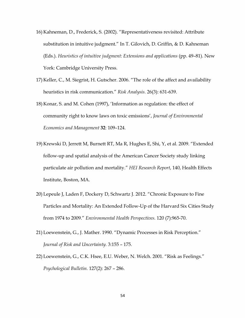
54

16) Kahneman, D., Frederick, S. (2002). “Representativeness revisited: Attribute

substitution in intuitive judgment.” In T. Gilovich, D. Griffin, & D. Kahneman

(Eds.). Heuristics of intuitive judgment: Extensions and applications (pp. 49–81). New

York: Cambridge University Press.

17) Keller, C., M. Siegrist, H. Gutscher. 2006. “The role of the affect and availability

heuristics in risk communication.” Risk Analysis. 26(3): 631-639.

18) Konar, S. and M. Cohen (1997), ‘Information as regulation: the effect of

community right to know laws on toxic emissions’, Journal of Environmental

Economics and Management 32: 109–124.

19) Krewski D, Jerrett M, Burnett RT, Ma R, Hughes E, Shi, Y, et al. 2009. “Extended

follow-up and spatial analysis of the American Cancer Society study linking

particulate air pollution and mortality.” HEI Research Report, 140, Health Effects

Institute, Boston, MA.

20) Lepeule J, Laden F, Dockery D, Schwartz J. 2012. “Chronic Exposure to Fine

Particles and Mortality: An Extended Follow-Up of the Harvard Six Cities Study

from 1974 to 2009.” Environmental Health Perspectives. 120 (7):965-70.

21) Loewenstein, G., J. Mather. 1990. “Dynamic Processes in Risk Perception.”

Journal of Risk and Uncertainty. 3:155 – 175.

22) Loewenstein, G., C.K. Hsee, E.U. Weber, N. Welch. 2001. “Risk as Feelings.”

Psychological Bulletin. 127(2): 267 – 286.

55

23) New York Times. 2017.

https://www.nytimes.com/2017/02/05/us/politics/scott-pruitt-is-seen-

cutting-the-epa-with-a-scalpel-not-a-cleaver.html?mcubz=0&_r=0

24) Pittsburgh Post-Gazette, 2015a: http://www.post-

gazette.com/opinion/2015/12/01/It-s-time-to-clean-up-DTE-s-Shenango-

plant/stories/201512010011

25) Pittsburgh Post-Gazette, 2015b: http://www.post-

gazette.com/news/environment/2015/11/19/Regulators-reviewing-Shenango-

Coke-Works-compliance-with-2012-consent-decree/stories/201511190230

26) Pittsburgh Tribune Review (2014):

http://triblive.com/news/adminpage/5904612-74/pollution-agreement-

plant#axzz3u6v1ZKxH

27) Shenango Channel: http://shenangochannel.org/

28) Shiller, R. 2017. “Narrative Economics.” Presidential address delivered at the

129th annual meeting of the American Economic Association, January 7, 2017,

Chicago, IL.

29) Shimshak, J. 2014. “The Economics of Environmental Monitoring and

Enforcement: A Review,” Annual Review of Resource Economics. 6: 339–60.

30) Sargent, R., C. Bartley, P. Dille, J. Keller, and I. Nourbakhsh, ”Timelapse

GigaPan: Capturing, Sharing, and Exploring Timelapse Gigapixel Imagery,” in

Fine International Conference on Gigapixel Imaging for Science, 2010.

56

31) Slovic, P., Finucane, M. L., Peters, E., & MacGregor, D. G. (2002). “The affect

heuristic.” In T. Gilovich, D. Griffin, & D. Kahneman (Eds.), Heuristics and biases:

The psychology of intuitive judgment (pp. 397-420). New York: Cambridge

University Press.

32) Tietenberg, T.H. (1998), ‘Disclosure strategies for pollution control’,

Environmental and Resource Economics. 11: 587–602.

33) United States Environmental Protection Agency (USEPA). 2017.

https://www.epa.gov/outdoor-air-quality-data/air-quality-index-report

57

Appendix.

58

Figure A.1. Histograms of Wind Direction at Avalon Monitor.

Left Panel: Hourly wind direction from March, 2015 through November, 2015. Right

Panel: Hourly wind direction during spring 2015 power outage.

59

Figure A.2. PM2.5 and Wind Direction.

Left Panel: Hourly PM2.5 Observations. Right Panel: Average PM2.5 Readings.

Vertical line = orientation of main stack at Shenango and Avalon monitor.

60

Figure A.3: Smoke Detection Algorithm.

61

Figure A.4: Sample of Time Lapse View and Data Depiction.

62

Figure A.5: Smoke Detection Results for May 2, 2015.

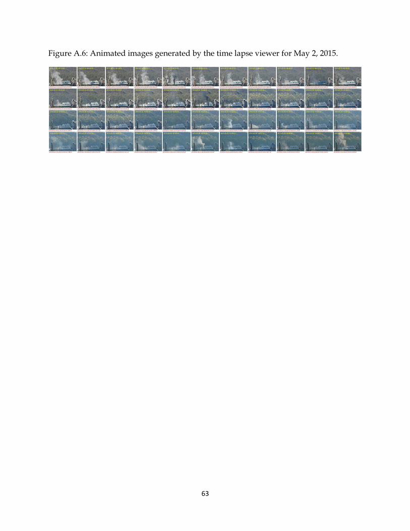
63

Figure A.6: Animated images generated by the time lapse viewer for May 2, 2015.

64

Table A1: Comparison of PM2.5 Levels at Avalon Monitor Before and After Camera.

Wind Direction (Degrees)

Before Camera

After Camera

Percent Change

t-stat (p-value)

Obs. Before/ Obs. After

205 - 215 13.793A 11.193 18.85 2.568 (0.005)

116/135

200 – 220 13.862 12.649 8.75 1.937 (0.027)

443/387

195 – 225 13.904 13.038 6.23 1.595 (0.055)

636/551

175 - 245 14.340 13.293 7.30 3.122 (0.001)

1,446/1,305

165 - 255 14.184 13.234 6.70 3.419 (0.000)

1,990/1,771

A = before and after camera activation measurements of PM2.5 expressed in ug/m3.

65

Table A2: Full Regression Model Results for All Calls to ACHD.

Covariates

(1) (2) (3) (4)

Cam. On -0.0250 -0.0759 -0.0302 -0.0488 (0.201) (0.224) (0.226) (0.175)

Cam. Active 0.462*** 0.233 -0.944 -0.827 (0.0823) (0.247) (1.409) (1.171)

Closure -1.390*** -1.366*** -1.254*** (0.285) (0.286) (0.246)

Article 0.654 0.765 0.662*** (0.519) (0.540) (0.148)

Meeting -0.532 -0.571 -0.629* (0.464) (0.469) (0.346)

PM2.5 0.0216 0.161 0.140 (0.100) (0.158) (0.135)

SO2 0.119** 0.0866 0.0915 (0.0498) (0.0714) (0.0637)

O3 -0.0258 0.111 0.125 (0.135) (0.217) (0.175)

Incident -0.0657 -0.0807 -0.0493 (0.203) (0.200) (0.150)

spring -0.388** -0.358** -0.332** (0.166) (0.166) (0.142)

summer -0.586*** -0.569*** -0.485*** (0.188) (0.185) (0.154)

fall -0.320** -0.278* -0.213* (0.154) (0.155) (0.125)

Day of sample 0.00767*** 0.00595** 0.00545** (0.00226) (0.00266) (0.00236)

(Day of sample)2 -0.0000191** -0.0000122 -0.0000112 (0.00000835) (0.0000100) (0.00000863)

(Day of sample)3 1.53e-08** 8.94e-09 8.01e-09 (7.59e-09) (9.12e-09) (7.78e-09)

Temperature 0.0236** 0.0222** 0.0227*** (0.00919) (0.00922) (0.00760)

Temperature2 -0.0000121 0.0000273 -0.000161 (0.000390) (0.000387) (0.000332)

Wind 0.00271 0.000682 0.00626 Direction (0.00441) (0.00559) (0.00442) Wind -0.00000629 -0.00000279 -0.0000142 Direction2 (0.0000109) (0.0000137) (0.0000108)

66

Wind -0.0449 -0.0142 -0.0247 Speed (0.0905) (0.0904) (0.0722) Wind 0.00949 0.00674 0.00659 Speed2 (0.00772) (0.00764) (0.00619) Camera x PM2.5 -0.237 -0.154

(0.185) (0.159) Camera x SO2 0.0677 0.0582

(0.0997) (0.0853) Camera x O3 -0.234 -0.271

(0.275) (0.226) Camera x Wind 0.00601 -0.00151 Direction (0.00812) (0.00667) Camera x Wind -0.0000117 0.00000445 Direction2 (0.0000201) (0.0000166) Camera x Monday 0.310**

(0.143) Camera x Weekday 0.582***

(0.0893) Monday 1.648***

(0.100) Weekday 1.060***

(0.0639) Constant 1.009*** -0.419 0.00154 -1.421

(0.0565) (0.708) (1.084) (0.892)

Ln(alpha) -0.526*** -0.698*** -0.710*** -1.429*** (0.0652) (0.0640) (0.0634) (0.104)

N 730 727 727 727 Standard errors in parentheses: * p<0.10, ** p<0.05, *** p<0.01 Dependent Variable is daily count of all calls to ACHD pertaining to air pollution.

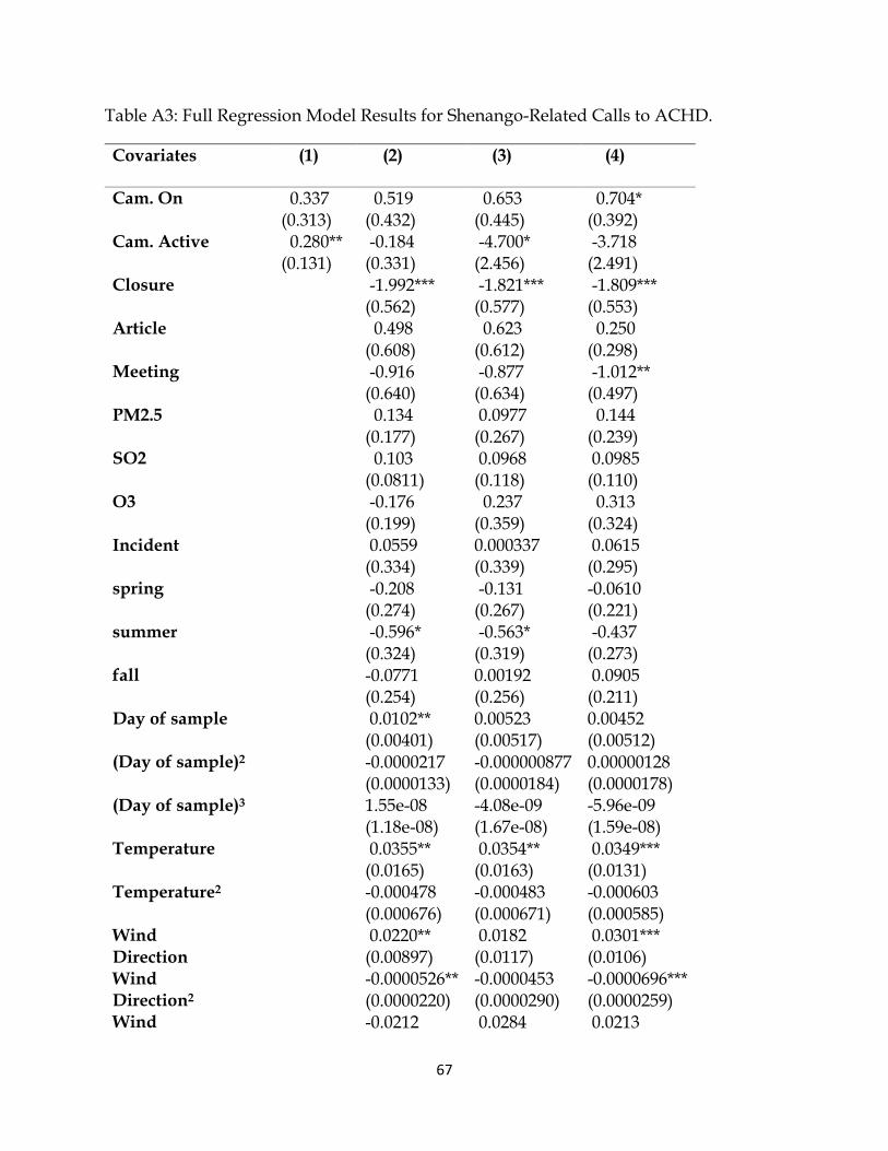
67

Table A3: Full Regression Model Results for Shenango-Related Calls to ACHD.

Covariates

(1) (2) (3) (4)

Cam. On 0.337 0.519 0.653 0.704* (0.313) (0.432) (0.445) (0.392)

Cam. Active 0.280** -0.184 -4.700* -3.718 (0.131) (0.331) (2.456) (2.491)

Closure -1.992*** -1.821*** -1.809*** (0.562) (0.577) (0.553)

Article 0.498 0.623 0.250 (0.608) (0.612) (0.298)

Meeting -0.916 -0.877 -1.012** (0.640) (0.634) (0.497)

PM2.5 0.134 0.0977 0.144 (0.177) (0.267) (0.239)

SO2 0.103 0.0968 0.0985 (0.0811) (0.118) (0.110)

O3 -0.176 0.237 0.313 (0.199) (0.359) (0.324)

Incident 0.0559 0.000337 0.0615 (0.334) (0.339) (0.295)

spring -0.208 -0.131 -0.0610 (0.274) (0.267) (0.221)

summer -0.596* -0.563* -0.437 (0.324) (0.319) (0.273)

fall -0.0771 0.00192 0.0905 (0.254) (0.256) (0.211)

Day of sample 0.0102** 0.00523 0.00452 (0.00401) (0.00517) (0.00512)

(Day of sample)2 -0.0000217 -0.000000877 0.00000128 (0.0000133) (0.0000184) (0.0000178)

(Day of sample)3 1.55e-08 -4.08e-09 -5.96e-09 (1.18e-08) (1.67e-08) (1.59e-08)

Temperature 0.0355** 0.0354** 0.0349*** (0.0165) (0.0163) (0.0131)

Temperature2 -0.000478 -0.000483 -0.000603 (0.000676) (0.000671) (0.000585)

Wind 0.0220** 0.0182 0.0301*** Direction (0.00897) (0.0117) (0.0106) Wind -0.0000526** -0.0000453 -0.0000696*** Direction2 (0.0000220) (0.0000290) (0.0000259) Wind -0.0212 0.0284 0.0213

68

Speed (0.149) (0.151) (0.131) Wind 0.0117 0.00726 0.00609 Speed2 (0.0125) (0.0126) (0.0110) Camera x PM2.5 0.0682 0.142

(0.305) (0.290) Camera x SO2 0.00928 0.0325

(0.155) (0.139) Camera x O3 -0.761* -1.038**

(0.451) (0.439) Camera x Wind 0.0131 -0.00311 Direction (0.0152) (0.0137) Camera x Wind -0.0000274 0.00000766 Direction2 (0.0000376) (0.0000338) Camera x Monday -0.706

(0.893) Camera x Weekday -0.249

(0.886) Monday 5.099***

(0.703) Weekday 4.236***

(0.697) Constant 0.130 -4.605*** -2.631 -7.899***

(0.0990) (1.288) (1.869) (1.854)

Ln(alpha) 0.882*** 0.666*** 0.657*** -0.188 (0.0905) (0.0970) (0.0967) (0.131)

N 730 727 727 727 Standard errors in parentheses: * p<0.10, ** p<0.05, *** p<0.01 Dependent Variable is daily count of all calls to ACHD pertaining to Shenango Mill.

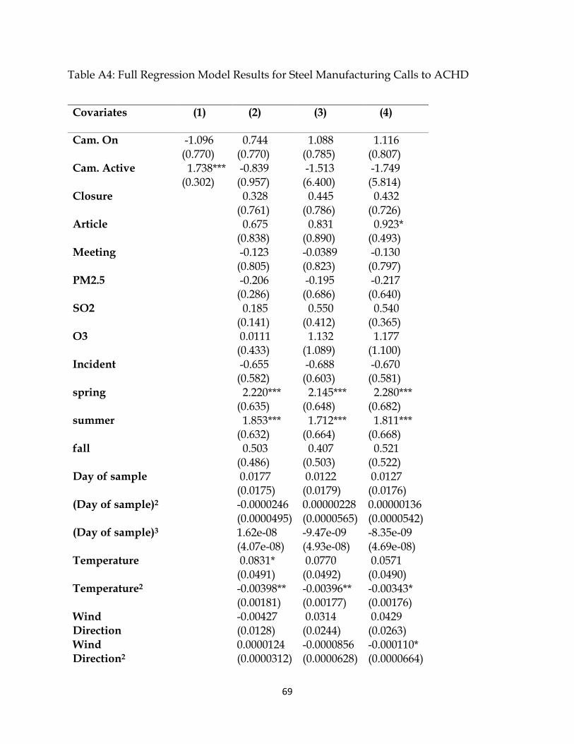
69

Table A4: Full Regression Model Results for Steel Manufacturing Calls to ACHD

Covariates

(1) (2) (3) (4)

Cam. On -1.096 0.744 1.088 1.116 (0.770) (0.770) (0.785) (0.807)

Cam. Active 1.738*** -0.839 -1.513 -1.749 (0.302) (0.957) (6.400) (5.814)

Closure 0.328 0.445 0.432 (0.761) (0.786) (0.726)

Article 0.675 0.831 0.923* (0.838) (0.890) (0.493)

Meeting -0.123 -0.0389 -0.130 (0.805) (0.823) (0.797)

PM2.5 -0.206 -0.195 -0.217 (0.286) (0.686) (0.640)

SO2 0.185 0.550 0.540 (0.141) (0.412) (0.365)

O3 0.0111 1.132 1.177 (0.433) (1.089) (1.100)

Incident -0.655 -0.688 -0.670 (0.582) (0.603) (0.581)

spring 2.220*** 2.145*** 2.280*** (0.635) (0.648) (0.682)

summer 1.853*** 1.712*** 1.811*** (0.632) (0.664) (0.668)

fall 0.503 0.407 0.521 (0.486) (0.503) (0.522)

Day of sample 0.0177 0.0122 0.0127 (0.0175) (0.0179) (0.0176)

(Day of sample)2 -0.0000246 0.00000228 0.00000136 (0.0000495) (0.0000565) (0.0000542)

(Day of sample)3 1.62e-08 -9.47e-09 -8.35e-09 (4.07e-08) (4.93e-08) (4.69e-08)

Temperature 0.0831* 0.0770 0.0571 (0.0491) (0.0492) (0.0490)

Temperature2 -0.00398** -0.00396** -0.00343* (0.00181) (0.00177) (0.00176)

Wind -0.00427 0.0314 0.0429 Direction (0.0128) (0.0244) (0.0263) Wind 0.0000124 -0.0000856 -0.000110* Direction2 (0.0000312) (0.0000628) (0.0000664)

70

Wind 0.306 0.261 0.240 Speed (0.456) (0.398) (0.347) Wind -0.0329 -0.0293 -0.0268 Speed2 (0.0460) (0.0425) (0.0351) Camera x PM2.5 -0.0487 0.0286

(0.702) (0.673) Camera x SO2 -0.427 -0.407

(0.436) (0.395) Camera x O3 -1.307 -1.280

(1.247) (1.245) Camera x Wind -0.0373 -0.0509* Direction (0.0282) (0.0297) Camera x Wind 0.000104 0.000134* Direction2 (0.0000720) (0.0000749) Camera x Monday 1.026*

(0.536) Camera x Weekday 1.530***

(0.487) Monday 16.18***

(0.461) Weekday 15.45***

(0.343) Constant -3.064*** -7.361** -7.408 -23.72***

(0.265) (3.285) (5.815) (5.327)

Ln(alpha) 1.025*** 0.625* 0.517 -0.0739 (0.301) (0.349) (0.350) (0.420)

N 730 727 727 727 Standard errors in parentheses. * p<0.10, ** p<0.05, *** p<0.01 Dependent Variable is daily count of Steel Manufacturing calls to ACHD pertaining to air pollution.

71

Table A5: Comparison of Different Estimators for All Calls to ACHD.

Covariates

(1) OLS

(2) Neg. Bin.

(3) Poisson

Camera On -0.146 -0.0488 -0.0571 (0.780) (0.175) (0.198)

Closure -5.027*** -1.254*** -1.338*** (1.261) (0.246) (0.248)

Article 6.170*** 0.662*** 0.697*** (2.367) (0.148) (0.167)

Camera Active -5.682 -0.827 -0.954 (5.436) (1.171) (1.332)

Camera x Monday 1.918* 0.310** 0.283* (0.979) (0.143) (0.151)

Camera x Weekday 2.448*** 0.582*** 0.583*** (0.405) (0.0893) (0.0944)

Monday 4.372*** 1.648*** 1.679*** (0.585) (0.100) (0.105) Weekday 1.961*** 1.060*** 1.084*** (0.208) (0.0639) (0.0680) Constant -2.534 -1.421 -1.507

(3.496) (0.892) (1.058) Season Fixed X X X Effects Cubic Time X X X Trend Weather X X X Controls Monitor X X X Pollution Camera x X X X Monitor Pollution

lnalpha -1.429*** (0.104)

Adj. R2 0.306 N 727 727 727

Standard errors in parentheses Note:* p<0.10, ** p<0.05, *** p<0.01

72

Table A6: Comparison of Different Estimators for Shenango-Related Calls to ACHD.

Covariates

(1) OLS

(2) Neg. Bin.

(3) Poisson

Camera On 0.643 0.704* 0.389 (0.610) (0.392) (0.325)

Closure -1.907*** -1.809*** -1.899*** (0.595) (0.553) (0.504)

Article 1.884*** 0.250 0.359 (0.439) (0.298) (0.264)

Camera Active -5.420* -3.718 -2.340 (3.000) (2.491) (2.355)

Camera x Monday 0.133 -0.706 -0.766 (0.599) (0.893) (0.936)

Camera x Weekday 0.703*** -0.249 -0.293 (0.242) (0.886) (0.925)

Monday 2.807*** 5.099*** 5.075*** (0.451) (0.703) (0.713) Weekday 1.276*** 4.236*** 4.223*** (0.151) (0.697) (0.704) Constant -3.040 -7.899*** -7.336***

(2.371) (1.854) (1.991) Season Fixed X X X Effects Cubic Time X X X Trend Weather X X X Controls Monitor X X X Pollution Camera x X X X Monitor Pollution

Ln(alpha) -0.188 (0.131)

Adj. R2 0.234 N 727 727 727 Standard errors in parentheses Note:* p<0.10, ** p<0.05, *** p<0.01

73

Table A7: Comparison of Different Estimators for Steel Manufacturing Calls to ACHD.

Covariates

(1) OLS

(2) Neg. Bin.

(3) Poisson

Camera On 0.0201 1.116 1.103 (0.0631) (0.807) (0.828)

Closure 0.207 0.432 0.422 (0.168) (0.726) (0.750)

Article 0.378 0.923* 0.975** (0.256) (0.493) (0.488)

Camera Active -0.366 -1.749 -1.710 (0.721) (5.814) (6.012)

Camera x Monday 0.274*** 1.026* 1.205** (0.0965) (0.536) (0.480)

Camera x Weekday 0.268*** 1.530*** 1.687*** (0.0594) (0.487) (0.373)

Monday 0.124*** 16.18*** 15.26*** (0.0449) (0.461) (0.452) Weekday 0.0759*** 15.45*** 14.59*** (0.0220) (0.343) (0.356) Constant 0.0897 -23.72*** -22.90***

(0.241) (5.327) (5.407) Season Fixed X X X Effects Cubic Time X X X Trend Weather X X X Controls Monitor X X X Pollution Camera x X X X Monitor Pollution

Ln(alpha) -0.0739 (0.420)

Adj. R2 0.100 N 727 727 727 Standard errors in parentheses Note:* p<0.10, ** p<0.05, *** p<0.01