WP-2012-015

Political Strongholds and Budget Allocation for Developmental

Expenditure: Evidence from Indian States, 1971-2005

Arun Kaushik and Rupayan Pal

Indira Gandhi Institute of Development Research, Mumbai

June 2012

http://www.igidr.ac.in/pdf/publication/WP-2012-015.pdf

Political Strongholds and Budget Allocation for Developmental

Expenditure: Evidence from Indian States, 1971-2005

Arun Kaushik and Rupayan Pal

Indira Gandhi Institute of Development Research(IGIDR) General Arun Kumar Vaidya Marg

Goregaon (E), Mumbai- 400065, INDIA Email (corresponding author): rupayan@igidr.ac.in

Abstract

This paper examines the effects of political factors on allocation of revenue budget for developmental

expenditure by the sub-national governments, using data from 15 major states in India during the

period 1971-2005. It measures the ruling party’s political stronghold on the basis of constituency level

electoral outcomes and shows that greater stronghold of the ruling party in a state leads to

significantly higher proportion of revenue budget allocated for developmental expenditure. It also

shows that voters’ turnout and political regime change have positive and significant effect on

proportion of revenue budget allocated for developmental expenditure. However, political ideology,

within government fragmentation, disproportionality in representation, and effective number of political

parties do not have any significant impact on budget allocation decisions of the Indian state

governments. Results of this paper also indicate that greater reliance on market forces reduces the

share of developmental expenditure. These are new and robust results.

Keywords: Political stronghold, budget allocation, developmental expenditure, state government,

ruling party, political factors, India

JEL Classifications: D72, H72, D71

Acknowledgements: We would like to thank Karl Schlag and Elena Esposito for helpful comments

and discussions. Usual disclaimer applies.

Arun Kaushik (arun.kaushik@unibo.it) is with University of Bologna, Italy

1  

Political Strongholds and Budget Allocation for Developmental Expenditure: Evidence from Indian States, 1971-2005

Arun Kaushik‡ and Rupayan Pal††

‡ University of Bologna, Italy ††Indira Gandhi Institute of Development Research (IGIDR), India1

1. Introduction

Public expenditure may be defined as the value of goods and services bought by the State and its

articulations. It creates public endowments for the society and also generates positive

externalities to the economy. Apart from the volume of public expenditure, its composition is

considered to be an important factor for economic growth and development (Devarajan et al.,

1996; Hong and Ahmed, 2009; Cozzi and Impullitti, 2010). In a democracy composition of

public expenditure is expected to represent people’s will. However, political-institutional

incentives are likely to distort the allocation of budget for different categories of public

expenditure.

It is also well recognized that developmental expenditures by the state governments are robust

determinants of poverty reductions across Indian states (e.g., Dutt and Ravallion, 2002; Hong

and Ahmed, 2009). Results of cross-country studies further reinforce the argument that

developmental expenditure has serious repercussions to growth and development, particularly in

case of developing countries (Gupta et al., 2002; Rajkumar and Swaroop, 2008). The purpose of

this paper is to examine the effects of various political factors on allocation of revenue budget for

developmental expenditure by the state governments in India. To be more specific, this paper

attempts to answer the following questions, using data from 15 major states in India during 1971-

2005. Does the extent of political stronghold of the ruling party in a state affect the share of

revenue budget allocated for developmental expenditure? Is there any effect of voter’s turn out,

effective number of political parties, political regime change, political ideology, form and                                                             1 Corresponding Author and Address: Rupayan Pal, Indira Gandhi Institute of Development Research (IGIDR), Film City Road, Gen A. K. Vaidya Marg, Goregaon (East), Mumbai 400065, India. E-mails: †† rupayan@igidr.ac.in, rupayanpal@gmail.com ; ‡ arun.kaushik@unibo.it Telephone: +91-22-28416545, Fax: +91-22-28402752.  

2  

representativeness of the government, president’s rule, and economic liberalization on

government’s preference for developmental expenditure?

The choice of state governments in India for the purpose of the present analysis rests on several

considerations. First, India is the world’s largest democracy and is federal in structure. Indian

states are empowered with partial policy autonomy and there is diverse pattern of growth and

development across states. Second, states in India widely differ in terms of political factors,

despite having a common electoral law. Third, sub-national governments within a country share

a more common institutional framework, unlike national governments of different countries,

which makes the present analysis more effective than cross-country studies.

There is a large number of cross-country studies that attempt to examine the implications of

political factors to government size and policy formulation (see, for example, Barro, 1991;

Alesina et al, 1992; Baskaran 2011; Potrafke, 2011). Existence of federal states within a country

adds an additional dimension. For example, Arulampalam et al (2009) argue that the central

government of India being opportunistic makes the transfers to states based on political

considerations, which in turn affects the size of the state governments. This paper deviates away

from the issues related to government size and center-state transfers in order to focus on the

allocation of revenue budget by the state governments.

We also note here that few studies have attempted to examine the determinants of government

expenditure in the context of Indian states. However, most of these studies have primarily

focused on existence of political business cycles at sub-national levels (e.g., Khemani 2004; Saez

and Sinha, 2009). Lalvani (2005) examines the implications of the form of government, coalition

or single party, on state governments’ fiscal policies during the period 1966-1998, but abstains

from examining budget allocation decisions. Uppal (2011) examines impact of legislative

turnover on government size and allocation of budget between capital expenditure and revenue

expenditure. On the other hand, Chhibber and Nooruddin (2004) examine state governments’

preferences for developmental expenditure during the period 1967-1997. However, unlike the

present paper, Chhibber and Nooruddin (2004) considers only a subset of the political factors

and, thus, fail to recognize possible implications of factors such as political stronghold of the

3  

ruling party, political regime change, president’s rule, and representativeness of the legislative

assembly of the state. The analysis of this paper is more comprehensive and it provides fresh

evidence of the effects of various political factors on allocation of revenue budget by the sub-

national governments of a developing country.

This paper constructs a new measure of political stronghold of the ruling party in a state, which

is based on constituency level data on electoral outcome, and examines its impact along with that

of other factors on state governments’ preferences for developmental expenditure over non-

developmental expenditure. Econometric analysis of this paper reveals that political stronghold

of the ruling party in a state is an important determinant of the allocation of revenue budget for

developmental expenditure in a state. A notable result is that greater political stronghold of the

ruling party in a state leads to higher proportion of revenue budget allocated for developmental

expenditure in that state. It seems to support the argument that higher possibility to retain the

office induces the incumbent ruling party to be more accountable to citizens (Ferraz and Finan,

2011). This result remains valid, if we consider alternative measures of political stronghold, and

it is not sensitive to the specification of the econometric model considered.

Analysis of this paper also reveals several other interesting results. It shows that political regime

change, i.e. change of the political party in power, has significant positive impact on the share of

revenue budget allocated for developmental expenditure. In other words, persistence of a

particular political party in power seems to be detrimental for a state, as far as developmental

expenditure is concerned. Moreover, results of this paper indicate that higher level of political

participation of citizens in a state can lead to stronger preference for developmental expenditure,

vis-à-vis non-developmental expenditure, of that state’s government. It also shows that the extent

of disproportional representation in the legislative assembly does not have any significant effect

on revenue budget allocation by the state government. Further, it demonstrates that liberalization

of the Indian economy has adversely affected the share of revenue budget allocated for

developmental expenditure by the state governments. These are new results. In contrast to the

findings of the existing studies, this paper shows that (a) the form of the government, coalition or

single party, i.e. within government fragmentation, (b) effective number of political parties, (c)

4  

political ideology and (d) president’s rule do not have any significant effect on budget allocation

decisions.

The rest of the paper is organized as follows. The next section describes the data and the

variables considered in this analysis. Section 3 presents the econometric model and estimation

methodology. Section 4 reports and discusses the estimation results. Section 5 concludes.

2. Data and Variables

For the purpose of the present analysis we consider 15 major states in India, namely, Andhra

Pradesh, Assam, Bihar, Gujarat, Haryana, Karnataka, Kerala, Madhya Pradesh, Maharashtra,

Orissa, Punjab, Rajasthan, Tamil Nadu, Uttar Pradesh and West Bengal, for the period 1971-

2005. These 15 states cover about 90% of India’s population. This analysis is based on data from

various sources. Data on state government’s expenditure is collated from Handbook of State

Finances 2010 published by Reserve Bank of India for the years 1990-2005, and from Besley

and Burgess (2002) for the earlier years. To measure the political factors, we use data from the

statistical reports of general elections to the legislative assemblies of various states, issued by the

Election Commission of India, and official websites of various state governments.

Dependent Variable: The dependent variable is the percentage of revenue expenditure allocated

for developmental expenditure by a state government in a year. We mention here that the state

governments’ budget for revenue expenditure has three components: (a) developmental

expenditure, (b) non-developmental expenditure and (c) grants-in-aid and contributions to local

bodies and institutions. Developmental expenditure comprises of expenditure on various social

services, such as health, education, family welfare, sanitation, social security, etc., and

expenditure on economic services provided for agriculture and allied activities, rural

development, irrigation, special area programs, energy supply, village and small industries

development, tourism development, etc. On an average, 64.88% of revenue expenditure has been

allocated for developmental expenditure by the state governments during the period of study

1971-2005 (see Table 1A).

5  

Table 1A: Summary Statistics Variables

Number of Observations

Mean

Standard Deviation

Maximum

Minimum

Developmental Expenditure as a Percentage of Revenue expenditure 525 64.88 7.68 79.8 36.29 Stronghold 525 25.24 15.91 65.81 0 Coalition Govt. 525 0.326 0.47 1 0 Alteration in Power 525 0.659 0.47 1 0 Voter Turnout 525 62.86 9.89 87.9 23.8 Ideological Stand of Parties 525 0.065 0.49 1 -1 President Rule 525 0.103 0.3 1 0 ENP 525 2.69 1.19 7.39 1.41 ENPv 525 3.97 1.21 8.46 2.29 DISPR 525 17.24 6.56 31.38 4.26

Interestingly, we observe that there is wide variation in terms of share of developmental

expenditure across states and over time. We depict the five year average values of shares of

developmental expenditures across states for four sub-periods in Figure 1. It seems that the

relative importance, as perceived by the state governments, of developmental expenditure vis-à-

vis non-developmental expenditure and grants-in-aid has undergone substantial changes over

time in all the states. In most of the states the share of developmental expenditure has been

reduced after 1981-85, though the scale of reduction differs across states. Also, note that even the

range of average of the percentage of revenue expenditure allocated for developmental

expenditure during the period of study is quite large, with the highest in Gujarat (69.60%) and

lowest in Punjab (59.98%), see Table 1B. In the last year of the period of study, i.e., in 2005, the

share of developmental expenditure was only 40.19% in Punjab, while that in Haryana was about

61.8%.

Explanatory Variables: Since the focus of this paper is to examine political factors affecting

allocation of revenue expenditure’s budget for developmental expenditure by the state

governments, we construct several variables to control for different aspects of political factors

and institutions.

 

Fi

Strongho

political

evident t

that cons

constitue

necessary

a party h

vis-à-vis

or equal

strongho

Note tha

constitue

strength o

contested

igure 1: Dev

old: First and

stronghold

that, if an el

stituency sea

encies in wh

y, but not su

has stronghol

other partie

to an appro

ld of that po

at the streng

ency’s electio

of that party

d for the sea

velopmental

d foremost,

of the majo

lectoral cons

at. However

hich it won.

ufficient, con

ld in a const

es in that con

opriately de

olitical party.

gth of a pol

on results. O

y. However,

at as well as

l Expenditu

we construc

or ruling par

stituency is

r, a political

In other w

ndition to cal

tituency or n

nstituency. I

efined critica

.

litical party

One may arg

vote share o

s on relative

6 

ure as a perc

ct the variab

rty in a state

stronghold

party need n

words, winni

ll that consti

not that depe

If a party’s s

al value ( z) )

in a consti

gue that high

of a party is l

e strengths o

centage of R

ble Strongho

e governmen

of a politica

not necessar

ng of a con

ituency as str

ends on the r

strength in a

), we may c

ituency is li

her vote shar

likely to dep

of contestan

Revenue Exp

ld to examin

nt to budget

al party, tha

rily have stro

nstituency se

ronghold of

relative stren

a constituenc

call that con

ikely to be

re of a party

pend on the n

nts. In a mu

penditure

ne the role o

t allocation.

at party must

onghold in a

eat by a par

f a party. Wh

ngth of that

cy is greater

nstituency a

reflected in

indicates gr

number of pa

lti-party pol

 

of the

It is

t win

all the

rty is

hether

party

r than

as the

n that

reater

arties

litical

7  

system as in India, the winning party of constituency i may have higher vote share, but lower

winning margin, compared to that of the winning party of constituency j. While higher vote share

indicates greater strength, lower winning margin indicates closer contest and, thus, lower

strength of the winning party. Therefore, higher vote share need not necessarily imply greater

strength. Winning margin should also be taken in to account, along with the vote share, to

measure strength of the winning party of any constituency.

Suppose party A wins in constituency i and party B wins in constituency j. Party A and Party B

may be the same party or different parties. Then, (a) for any given winning margin, if the vote

share of party A in constituency i is higher than that of party B in constituency j, strength of

party A in constituency i is greater than the strength of party B in constituency j; (b) for any

given vote share, if the winning margin of party A in constituency i is higher than that of party B

in constituency j, strength of party A in constituency i is greater than the strength of party B in

constituency j; and (c) if the winning margin (vote share of the winning party) in a constituency

increases, the rate of increase in strength of the winning party in that constituency due to increase

in vote share (winning margin) should also increase. That is, the measure of strength, z, of the

winning party in a constituency must satisfy the following three properties.

(A1) 0>∂∂

i

i

vz ,

(A2) 0>∂∂

i

i

mz and

(A3) 0,0 >⎟⎟⎠

⎞⎜⎜⎝

⎛∂∂

∂∂

>⎟⎟⎠

⎞⎜⎜⎝

⎛∂∂

∂∂

i

i

ii

i

i mz

vvz

m;

where zi, vi and mi denote the strength of the winning party, vote share of the winning party and

winning margin, respectively, in constituency i. In other words, any function ),( iii mvfz = that

satisfies the (A1)-(A3), can be considered as a measure of strength of the winning party in

constituency i. For simplicity, we can consider that iiiii mvmvfz == ),( . Therefore, if

zmvz iii)≥= , we can say that the constituency i is a stronghold of its winning party.

8  

Now, note that there is no obvious way to define the critical value z) . It seems to be more

convincing to set the critical value based on observed values of z, instead of considering some

arbitrary z) . Thus, we can consider that [ ] 0,100

1)( ≥⎥⎦⎤

⎢⎣⎡ += hwherehzmeanz) . That is, for a

constituency to be stronghold of a party, that party must win that constituency seat and the

strength of that party in that constituency must be greater than or equal to (some multiple of) the

average value of the strengths (zi) of all the winners in their respective constituencies in a state.

For the purpose of the present analysis, we first consider that h =0. We also consider alternative

values of h to check robustness of our results.

We define the measure Stronghold ( wS ) as the percentage of constituencies in which the ruling

party of a state has stronghold. That is, 1001

nn

S w = , where n is the total number of electoral

constituencies in a state and n1 ( n≤ ) in the number of constituencies in which the ruling party of

the state has stronghold, as defined above. Clearly, higher value of wS in a state indicates larger

number of safe constituencies for the ruling party of that state, i.e. the ruling party’s probability

to win in the next election is sufficiently high in larger number of constituencies.

We note here that, in the existing literature, a constituency is often considered as the stronghold

of a party, if that party has won all previous elections during a given period in that constituency.

See, for example, Khemani and Keefer (2009). However, such categorization does not appear to

be appropriate because of the following reasons. First, the results are likely to be different for

different length of the period considered, and there is no obvious way to choose the length of the

period. Second, it is quite plausible that a party wins a constituency in all the elections held

during a particular period of time by a negligible margin or merely by chance. Third,

delimitation of constituencies takes place at a regular interval in many countries including India,

which makes it difficult to trace a particular constituency over a reasonable time period.2

Delimitations often lead to significant changes in geographical boundaries of constituencies as

well as voters’ composition in constituencies to a large extent.

                                                            2 In India Article 82 of the Constitution directs Parliament to enact a Delimitation Act after every Census.

9  

Table 1B: States’ Profiles: 1971-2005

States N

o. o

f Obs

erva

tions

Shar

e of

Dev

elop

men

tal

Expe

nditu

re (

%)

Stro

ngho

ld (

%)

No.

of

Yea

rs u

nder

C

oalit

ion

Gov

t.

No.

of

Elec

tions

No.

of

Alte

ratio

ns i

n R

ulin

g P

arty

Vot

er T

urno

ut (

%)

No.

of

Yea

rs, w

hich

ha

d in

stan

ces o

f Pr

esid

ent

Rul

e

ENP V

ENP

DIS

PR

Andhra Pradesh 35 68.67 30.78 2 8 4 68.95 9 2.936 2.028 18.587 (5.568) (13.124) (2.97) (0.375) (0.301) (5.024)

Assam 35 65.33 29.32 15 7 6 69.32 8 3.791 2.541 16.656 (4.720) (15.318) (11.24) (1.194) (0.908) (5.973)

Bihar 35 62.34 19.66 12 7 6 58.03 9 5.535 3.486 14.725 (6.283) (7.509) (4.29) (1.088) (0.862) (3.853)

Gujarat 35 69.60 33.83 10 7 3 56.05 7 3.109 2.167 16.899 (5.637) (15.926) (5.82) (0.509) (0.764) (5.843)

Haryana 35 64.91 23.27 8 7 6 67.95 5 4.169 2.518 19.768 (9.327) (15.885) (3.05) (1.156) (0.647) (6.896)

Karnataka 35 66.30 26.94 2 8 5 66.93 8 3.378 2.267 17.552 (4.000) (13.840) (3.15) (0.608) (0.630) (5.995)

Kerala 35 64.50 3.66 35 7 7 74.53 7 6.534 5.737 8.933 (7.433) (2.466) (3.03) (0.848) (1.165) (3.624)

Madhya Pradesh 35 68.07 28.43 0 8 5 55.74 5 3.049 1.903 18.975 (5.401) (12.746) (5.56) (0.250) (0.323) (5.903)

Maharashtra 35 63.36 23.37 16 8 4 61.61 3 4.323 3.220 12.580 (5.748) (18.193) (5.09) (0.960) (1.276) (4.443)

Orissa 35 64.28 32.83 3 9 6 55.05 5 3.493 2.309 18.856 (7.839) (19.289) (9.95) (0.833) (0.894) (6.523)

Punjab 35 59.98 22.20 8 7 7 60.81 3 3.713 2.298 18.017 (13.310) (9.263) (15.44) (0.341) (0.376) (5.168)

Rajasthan 35 64.79 27.19 3 8 5 58.21 5 3.341 2.192 16.741 (5.654) (14.459) (7.27) (0.424) (0.531) (6.782)

Tamil Nadu 35 67.16 35.57 14 8 5 66.70 5 3.932 2.225 23.633 (7.469) (18.888) (4.97) (0.667) (0.511) (4.700)

Uttar Pradesh 35 60.56 12.95 13 9 7 51.39 9 4.712 2.990 15.999 8.159) (9.803) (4.80) (0.754) (0.988) (7.907)

West Bengal 35 62.09 28.56 30 7 1 71.68 4 3.594 2.492 20.652 (8.675) (10.815) (9.28) (0.520) (0.504) (5.629) Notes: Standard errors are in parenthesis. No. of years under president’s rule include the years of emergency (1975-1977) in India. ‘Left front’ is also considered as a coalition.

10  

It seems to be most appropriate to assess the voters’ attachment to a party through appropriately

designed survey of voters in order to examine whether a constituency is a stronghold of a

political party or not. If it is found that in a constituency, there is sufficiently large proportion of

voters attached to a party, that constituency may be considered as a stronghold of that party.

However, there is no such survey data available at constituency level in India, which renders it

impossible to directly asses the voter’s attachments to parties, and to measure a party’s strength

accordingly.

Higher level of political stronghold of the ruling party seems to indicate greater support base of

that party and, thus, higher possibility to be reelected. It is argued that higher reelection

possibility provides more incentive to a ruling party to be concerned about citizens’ welfare

(Ferraz and Finan, 2011). Therefore, higher political stronghold of the ruling party may induce

that party to be more concerned about developmental sectors. In contrast, one may argue that

higher reelection possibilities may induce the ruling party to perceive that its reelection

possibility does not depend on development in the state and, thus, allocate lower percentage of

revenue budget for developmental expenditure. Therefore, whether the effect of Stronghold on

share of developmental expenditure is positive or negative remains an empirical question.

We present the state-wise average of Stronghold (considering h =0), along with its standard

deviations, during 1971-2005 in Table 1B. The average of Stronghold was highest (35.57%) in

Tamil Nadu, followed by Gujarat and Orissa, and lowest (3.66%) in Kerala. Clearly, there was

wide variation in terms of political stronghold of the ruling parties across states. Further, there

was also large variation in Stronghold over time in most of the states, which is indicated by high

values of standard deviations of Stronghold.

Disproportional Representation (DISPR): It is well documented in the literature that all

democratically elected bodies are not necessarily equally representative, even if the voting rule is

the same (see, for example, Kaushik and Pal, 2012). Legislative assemblies of sates are also

likely to differ from each other in terms of their representativeness. A legislative assembly may

said to be perfectly representative, if each political party’s seat share in that legislative assembly

is equal to that party’s vote share. On the other extreme, if only one party gets all the seats

11  

without any voter’s support, we have a dictatorial regime. Following Gallagher (1991), we

consider the following measure of disproportional representation (DISPR), to examine the effect

of representativeness of legislative assemblies.

Disproportional Representation (DISPR) =

2

21100 ∑ ∑∑∈

∈∈ ⎥⎥⎥

⎦

⎤

⎢⎢⎢

⎣

⎡−

PjPk

k

j

Pkk

j

vv

ss

,

where sj denotes the number of seats of political party j in the legislative assembly, vj denotes the

number of votes received by the j-th political party and P denotes the set of political parties, in a

state in a year. Clearly, DISPR takes the value zero, if the legislative assembly is perfectly

representative. On the other extreme, if there is dictatorship, DISPR takes the value 100. Also, it

is easy to observe that DISPR is increasing in the extent of disproportion between seat share and

vote share. The average DISPR, taking all the states and years together, was 17.24, which

indicates that on an average the legislative assemblies of states were far from perfectly

representative. Nonetheless, as expected, representativeness of legislative assemblies varies

across states and over time (Table 1B). Average DISPR was lowest (8.93) in Kerala and highest

(23.63) in Tamil Nadu.

Electoral competition (ENPv and ENP): One may argue that, if the number of political parties

increases, competition faced by the political parties would be higher. However, note that all

parties are not necessarily equally strong. It is widely observed that there are variations across

political parties in terms of (a) their voters’ support base and (b)  number of seats won. It

indicates that increase in number of political parties does not necessarily mean increase in

competition in the election. Relative sizes of the political parties should be taken into account

while measuring electoral competition (Laakso and Taagepera, 1979). The percentage of votes

received by a political party as well as the number of seats won by a party can be viewed as the

size of that political party. Given this backdrop, effective number of political parties (ENPv),

which is defined as follows, may be considered as an appropriate measure of electoral

competition (Laakso and Taagepera, 1979).

12  

12 −

∈∈

⎥⎥⎥

⎦

⎤

⎢⎢⎢

⎣

⎡

⎟⎟⎟

⎠

⎞

⎜⎜⎜

⎝

⎛= ∑ ∑Pj

Pkk

jv v

vENP ,

where vj denotes the number of votes achieved by the j-th party and P is the set of political

parties. Clearly, ENPv takes into account the relative sizes of the political parties. It can be

interpreted as the number of hypothetical equal sized parties that would have the same total

effect on electoral competition as have the actual parties of unequal size. It is evident that the

lowest possible value of ENPv is one, when only one party gets all the votes. On the other

extreme, if all the parties get equal number of votes, ENPv is equal to the number of parties.

Clearly a higher value of ENPv indicates more intense competition among political parties in

election. We note here that this measure of competition in election has been widely used in the

literature (see, for example, Chhibber and Nooruddin, 2004; Saez and Sinha, 2009; Bortolotti

and Pinotti, 2008).

Note that the extent of competition in election can also be measured by considering share of seats

received by a party as its size. In that case, we need to replace vj by sj, in the above formula,

where sj, denotes the number of seats won by the j-th party. We denote this measure based on

seat share by ENP. Needless to mention here that the interpretation of ENP and its lower bound

and upper bound remains the same as that of ENPv . However, note that ENPv and ENP need not

necessarily be the same, unless vote share and seat share are same for all parties. To control for

possible effects of electoral competition, we consider these two alternative measures of electoral

competition in separate regressions. We report the descriptive statistics of these two measures of

competition in election in Table 1A and 1B.

Voter Turnout: We consider the variable Voter Turnout, which is measured as the percentage of

total number of voters casted their votes in an election for legislative assembly of a state, as the

proxy for citizens’ participation in the political process. Higher value of Voter Turnout indicates

more politically active citizens and, thus, greater political participation of citizens. It seems to be

likely that the extent of political participation of citizens would have effect on formation as well

as functioning of governments, which in turn would have effect on budget allocation decisions.

We observe that, on an average, Voter Turnout was about 63% in the sample states during the

13  

period of study, and it varied between 51.39% in Uttar Pradesh and 74.53% in Kerala (see Table

1A and Table 1B).

Alteration in Power: Normally, election for State Legislative Assembly takes place after every

five years in each of the Indian states. However, the year and the frequency of election differ

across states to some extent, depending on the internal political scenario of a state. During the

period of 35 years from 1971-2005, election for State Legislative Assembly took place seven

times in seven states, eight times in six states and nine times in two states, out of 15 states in the

sample. However, change of the major ruling party in the government, i.e., alteration in power,

took place less frequently than the frequency of election, except in Kerala and Punjab. In West

Bengal the major ruling party was altered only once, which is the least among all the states. See

Table 1B for state-wise number of changes in the major ruling party, which is defined as the

political party that formed the government or had the highest number of seats out of all the

political parties that formed the coalition government, during the period of study. If an

incumbent political party retains the power to govern a state, functioning of that state

government may be different from that in case there is a change of the ruling party. Therefore, to

control for possible effects of change in ruling party on budget allocation, we consider the

dummy variable Alteration in Power as an explanatory variable in the regression. The variable

Alteration in Power takes the value one if there is a change of major ruling party in the last

election; otherwise it takes the value zero.

Coalition Government: Single party governments may have different preferences for

developmental expenditure from that of multi-party coalition governments. We consider the

dummy variable Coalition Govt. to control for possible effects of coalition government.

Coalition Govt. takes the value one if there is a coalition government; otherwise it takes the

value zero. Descriptive statistics shows that there were coalition governments in significant

number of state-years, 117.15 out of 525. Except Madhya Pradesh, each of the other 14 states

was ruled by coalition government at some point of time or the other during 1971-2005.

Ideology Stand: It is often argued that ideological stands of political parties play important role

to shape government policies. Therefore, it seems to be important to control for possible effect of

14  

party ideology on developmental expenditure. To this effect, we first categorize the political

parties into three groups, namely, rightist, centrist and leftist, on the basis of their manifestos. We

consider (i) Bhartiya Janata Party (BJP) and Janata Party (JP) as rightist political parties, (ii)

Communist Party of India – Marxist (CPM), Communist Party of India (CPI), Communist Party

of India–Marxist-Leninist (CPIML), Forward Block (FB), Revolutionary Socialist Party (RSP),

Republican Party of India (RPI), Revolutionary Communist Party of India (RCPI), Party for

Democratic Socialism (PDS), All India Forward Block (AIFB) and Democratic Revolutionary

Peoples Party (DRPP) as leftist political parties, and (iii) all other political parties including

Indian National Congress (INC) as centrist political parties. Such categorization of political

parties in India is in line with the existing literature (see, for example, Pal 2010). We consider the

categorical variable Ideology Stand as an explanatory variable. Ideology Stand takes the value

one if the Chief Minister belongs to a rightist political party; it takes the value zero if the Chief

Minister belongs to a centrist political part; and it takes the value minus one (-1) if the Chief

Minister belongs to a leftist political party.

President Rule: Occasionally, elected government of a state was dissolved by the President of

India and then that state was governed by the President’s Rule until a new government was

formed, depending on internal socio-political situation of the state. There were instances of

President’s Rule in Andhra Pradesh, Bihar and Uttar Pradesh in nine out of 35 years, while in

Punjab and Maharashtra it was observed only in three out of 35 years. To control for possible

implications of such extra ordinary situations, we consider the variable President Rule, which

takes the value one if there is any instance of President’s Rule in a state in a year; otherwise it

takes the value zero.

We also consider (a) the dummy variables for the states to control of unobserved state-specific

factors and (b) either the dummy variables for the years to control for unobserved time-specific

effects or the dummy variable Liberalization Dummy to explicitly control for the possible effect

of economic liberalization in India, in alternative regressions, suitably. The variable

Liberalization Dummy takes the value one for post liberalization years, i.e., for 1991 and later

years; otherwise, it takes the value zero.

15  

3. Econometric Model and Estimation Methodology

We postulate the econometric model as follows.

)1(,ntntnt XY εβα ++= where n refers to state and t refers to year, n = 1, 2, 3, ... N and t = 1, 2, 3, ... T. The dependent

variable ntY is the logit transformation of ‘developmental expenditure as a percentage of revenue

expenditure ( ntZ )’, ntY is defined as )Z100

Zlog(Ynt

ntnt −= . Since ntZ is bounded between zero

and 100, and ntZ does not take any extreme value (zero or 100), considering logit transformation

of ntZ , as mentioned above, seems to be appropriate in order to conform to the normality

assumption. Nonetheless, if we consider standard log transformation of ntZ , our results do not

change. ntX denotes the vector of explanatory variables, β is the vector of coefficients of

explanatory variables and α is the intercept parameter, and ntε is the error term. We denote the

NTNT × variance-covariance matrix of the errors by Ω with typical element being )( jsntE εε ,

when the data are stacked by units (i.e., N time series are stacked).

It is well documented in the literature that there are several advantages in estimating models of

above mentioned type utilising both time series and cross-section data together, which is referred

as pooled time series cross-section (TSCS) analysis, rather than carrying out cross-section or

time series analysis separately. First, combining time series and cross-section data together

increases the number of observations, and thus, mitigates the ‘small N’ problem. Second, TSCS

analysis may rely upon higher variability of data compared to simple time series or cross-section

analysis. Third, TSCS analysis aims to capture the variations that emerge through two

dimensions, time and space, simultaneously.

The appropriate method of estimation of Model (1) depends on the structure of the variance-

covariance matrixΩ . If disturbances follow normal distribution; and 0)( =ntE ε , 22 )( σε =ntE ,

0)( =jtntE εε and there is no serial correlation, i.e., if disturbances are spherical, NTNT×=Ω I2σ ,

16  

ordinary least squares (OLS) provides consistent and efficient estimates of the parameters of the

model. However, in case of time series cross-section setting, variances of errors may vary across

states, i.e. errors may be heteroscedastic, errors may be contemporaneously correlated and/or

there may be serial correlation of errors, for instance, errors may follow AR(1) process. In other

words, error structure may be such that (a) 0)( =ntE ε , (b) 22 )( nntE σε = , (c) njjtntE σεε =)( , and

(d) nttnnt e+= − )1(ρεε , where 0)( =nteE , 2,

2 )( nenteE σ= and njejtnteeE ,)( σ= . Therefore, in the

present context, it is unlikely to have spherical disturbances. And, in case of non-spherical

disturbances, OLS provides consistent but inefficient estimates. Therefore, before estimating the

model, we need to test for existence of heteroscedasticity, contemporaneous correlation and

serial correlation. We perform widely used modified Wald test, Breusch-Pagan LM test and

Wooldridge test, respectively, to check for heteroscedasticity, contemporaneous correlation and

serial correlation. Results of these tests, reported in Table 4 in Appendix, confirm the presence of

heteroscedasticity, contemporaneous correlation and first order autocorrelation. It implies that,

disturbances are non-spherical and, thus, OLS estimates are not efficient.

To overcome the problem due to non-spherical disturbances, one can apply feasible generalized

least squares (FGLS) method in case of temporally dominant (i.e., NT > ) balanced panel data

without much difficulty, which provides consistent and efficient estimates of the parameters

(Greene 2003, Ch. 13; Baltagi 2008). To obtain FGLS estimates in presence of first order

autocorrelation, contemporaneous correlation and heteroscedasticity, we need to first estimate

the Model (1) by OLS and obtain the OLS residuals. Using the OLS residuals we can obtain

consistent estimate of autocorrelation parameter, ρ) . Then, we need to apply Prais-Winsten

transformation, using estimatedρ) , to transform the remainder AR(1) disturbances into serially

independent errors and to obtain consistent estimate of the variance-covariance matrix, Ω)

.

Finally, the Prais-Winsten transformed model is estimated by generalized least squares (GLS)

method using Ω)

.

Since we have data for 15 states over 35 years and there is no missing data, i.e, the data set is

temporally dominant and balanced panel, we employ FGLS method, taking in to account that

17  

there is heteroscedasticty, contemporaneous correlation and first-order autocorrelation, to

estimate Model (1) using alternative sets of explanatory variables.

It is argued that the above mentioned FGLS method of estimation may potentially underestimate

the standard errors of estimated coefficients of time series cross-section models, which makes the

FGLS estimation results unreliable (Beck and Katz 1995). Since OLS estimates are consistent,

but not efficient, Beck and Katz (1995) proposes to consider (a) OLS estimates of the

coefficients of the parameters, if there is no autocorrelation; and (b) coefficients of GLS

estimates of Prais–Winsten transformation of the model, if there is first order autocorrelation.

However, they propose to consider panel corrected standard errors (PCSE) that takes into

account the cotemporaneous correlation, serial correlation and heteroscedasticity, in order to

obtain reliable estimates of estimated coefficients’ standard errors. The proposed PCSEs are

based on a sandwich type estimator of the covariance matrix of the estimated parameters and are

robust to the possibility of non-spherical errors. Several studies, particularly in the fields of

comparative political science and sociology, have followed the suggestions of Beck and Katz

(1995). However, Beck and Katz (1995) also pointed out that it is less likely to have the

downward bias in standard errors of coefficient estimates from FGLS method, if the number of

time points (T) is substantially larger than the number of cross-sectional units (N). Note that, we

have T= 35 >> N=15. Therefore, the FGLS estimates are likely to be reliable in case of the

present study. Nonetheless, we estimate the models, corresponding to alternative specifications

as discussed before, following the suggestions of Beck and Katz (1995). The results of the Beck-

Katz estimates with PCSEs are reported in Table 5 in Appendix. We observe that results are not

sensitive to alternative estimation methodologies.

We also note here that one may argue in favor of inclusion of lagged dependent variable in the

model, since there is first order autocorrelation. However, if there is lagged dependent variable in

the set of explanatory variables, OLS estimates are biased and inconsistent. The appropriate way

to estimate dynamic panel data model seems to be by employing the generalized method of

moments (GMM), following Arellano and Bond (1991) or Blundell and Bond (1998). However,

the proposed GMM estimators of dynamic panel data models are designed for datasets with

many panels and few periods, i.e., for datasets in which N>>T., which renders Arellano and

18  

Bond (1991) and Blundell and Bond (1998) methodologies unsuitable in the present context.

Therefore, it is appropriate to consider OLS estimates, with PCSEs, of a model without any

lagged dependent variable in the present context, as suggested by Maddala et al (1997).

Nonetheless, if we consider lagged dependent variable as an explanatory variable in the model

and compute GMM estimates, main results of this analysis do not change substantially.

First, we consider Stronghold, Coalition Govt., Alteration in Power and Voter Turnout as

explanatory variables and estimate the model by FGLS method, the results of which are reported

in column (1) of Table 2. Next, we introduce Liberalisation Dummy as an additional explanatory

variable as reported in column (2) of Table 2, in order to examine the effects of liberalization of

Indian Economy and to examine the sensitivity of results in column (1). Third, we drop

Liberalisation Dummy and introduce Year Dummies, in order to control for time specific

unobserved effects. We do not consider Liberalization Dummy and Year Dummies together in the

regression to avoid the problem of multicollinearity. In other words, we estimate time-specific

fixed effects model by FGLS method, results of which are reported in column (3) of Table 2.

Fourth, we drop Year Dummies and consider State Dummies, which is the same as state-specific

fixed effects model, to examine the implications of state specific unobserved effects on

estimation results separately (see column (4) in Table 2). Fifth, we introduce Liberalisation

Dummy along with State Dummies in the set of explanatory variables, which helps us to examine

the effect of liberalization after controlling for state-specific unobserved effects, as reported in

column (5) in Table 2. Finally, we estimate the model after controlling for both state-specific

unobserved effects and time-specific unobserved effects. That is, we estimate the following

econometric model by FGLS method.

)2(,)()(1

1

1

1ntt

T

ttn

N

nnntnt DummyYearDummyStateXY εδγβα ++++= ∑∑

−

=

−

=

The variable nDummyState )( is dummy variable, which takes value 1 if the state is n, otherwise

it takes value zero; nγ is the coefficient of nDummyState )( . Similarly, tDummyYear )( is

dummy variable, which takes value 1 if the year is t, otherwise it takes value zero; tδ is the

coefficient of the dummy for year t. Clearly, Model (2) is the dummy variable representation of

two way fixed effects model. Estimation results of this model, when the vector ntX consists of

19  

(Stronghold, Coalition Govt., Alteration in Power and Voter Turnout), are reported in column (6)

of Table 2. We find that the results of FGLS estimation are robust to alternative specifications of

the model.

We also estimate the Model (2) considering alternative measures of the variable Stronghold, as

discussed in the previous section, by employing FGLS method and Beck-Katz method. See

Table 6 for the FGLS estimates and Table 7 for the Beck-Katz estimates, when alternative

measures of Stronghold have been considered. It is evident that the estimation results are not

sensitive to alternative methodologies considered.

Moreover, from Table 2 and Table 6, we can say that our results are not sensitive to the

measurement of Stronghold. Further, we estimate the Model (2) controlling for political ideology

of ruling party (Ideology Stand), president’s rule (President Rule), electoral competition (ENP,

ENPv) and disproportional representation in Legislative Assembly (DISPR). We find that the

main results of the analysis are robust to such alternative specifications as well (see Table 3).

Results of the present analysis also go through, if we consider post emergency period only, i.e. if

we consider the period from 1978 to 2005 (see, Table 8). In sum, it seems that our results are not

driven by the inclusion of data of pre-emergency and emergency periods together and our results

are robust to (a) alternative methodologies of estimation, (b) alternative specifications of the

model as well as (c) alternative measures of the variable Stronghold.

4. Estimation Results and Discussion

Table 2 presents the results of FGLS estimates of six different specifications of the model, as

discussed in Section 3. It is evident that the coefficients of Stronghold, Alteration in Power and

Voter Turnout are positive and significant, while the coefficient of Coalition Govt. is

insignificant and negative, irrespective of whether we control for state specific unobserved

effects and/or time specific unobserved effects or not. Moreover, these results do not change, if

we consider only the Liberalisation Dummy in place of Year Dummies. Further, the above

mentioned results remain unchanged, even if we control for other political variables that may

have implications to developmental expenditure (see Table 3). Also, since all the political

20  

variables used in the regression analysis were determined before the budget allocation decision

took place in any given year, the problem of endogeneity is less likely to occur in the present

analysis. Overall, it seems that these results are robust.

Table 2: Political Stronghold of Ruling Party and Developmental Expenditure

Dependent Variable: Logit transformation of ‘developmental expenditure as a percentage of revenue expenditure’

(1) (2) (3) (4) (5) (6)

Stronghold

0.0016*** [0.000]

0.0016*** [0.000]

0.0011*** [0.000]

0.0017*** [0.000]

0.0016*** [0.000]

0.0010*** [0.000]

Coalition Govt

-0.0047 [0.523]

-0.0098 [0.170]

-0.0037 [0.620]

-0.0055 [0.422]

-0.0087 [0.188]

-0.0010 [0.892]

Alteration in Power 0.0209*** [0.000]

0.0235*** [0.000]

0.0187*** [0.006]

0.0215*** [0.000]

0.0257*** [0.000]

0.0189*** [0.002]

Voter Turnout

0.0013** [0.005]

0.0014*** [0.001]

0.0012*** [0.005]

0.0012** [0.011]

0.0013*** [0.004]

0.0016*** [0.001]

Liberalisation Dummy -0.0922*** [0.000]

-0.0915*** [0.000]

Constant

0.1480*** [0.000]

0.1690*** [0.000]

-0.0299 [0.332]

0.0482 [0.396]

0.1040** [0.023]

-0.1180*** [0.004]

State Dummies No No No Yes Yes Yes

Year Dummies No No Yes No No Yes

Overall Significance Test: Wald Chi2 Prob. > Chi2

59.41 0.000

92.40 0.000

42505.40 0.000

178.60 0.000

384.70 0.000

101202.30 0.000

Number of Observations

525

525

525

525

525

525

Number of States 15 15 15 15 15 15

Time Periods 35 35 35 35 35 35

Common AR(1) Coefficient 0.7958 0.6661 0.6515 0.7681 0.5898 0.5153 Notes: Results are based on FGLS estimates. p-values are reported in brackets : * indicates p<0.1, ** indicates p<0.05, *** indicates p<0.01.

Note that the variable Stronghold measures the proportion of constituencies that are considered

to be safe by the ruling party. That is, higher value of Stronghold indicates that the probability of

the ruling party to be reelected in the next election is higher. A positive and significant

21  

coefficient of Stronghold seems to imply that the ruling party rewards the state by allocating

higher proportion of revenue budget for developmental expenditure, if the proportion of its safe

constituencies is higher. This result seems to be in line with the findings of Ferraz and Finan

(2011). Using data from Brazil, Ferraz and Finan (2011) show that Mayors with re-election

incentive are more accountable to citizens than the Mayors with less possibility of getting

reelected. In other words, concerns of the elected representatives for citizens’ welfare increase

with the increase in the probability of being reelected. Therefore, it seems that, on an average,

state governments with lower probability to be re-elected would be less concerned about

developmental works. This is in contrast to the view that lower probability of getting re-elected

makes the ruling party more active to enhance their chances to retain the power through

developmental works. Clearly, this is an interesting result.

We also find that there is positive and significant association of the dummy variable Alteration in

Power with the share of developmental expenditure. It supports our supposition that functioning

of a state government becomes different in case the incumbent ruling party is replaced by some

other political party, compared to the situation when the incumbent political party retains the

power to govern the state. If there is a change of the ruling party, the new ruling party allocates

higher proportion of revenue budget for developmental expenditure. It indicates that change of

political party in power is better for states, as far as developmental expenditure is concerned.

Positive and significant coefficient of Voter Turnout implies that higher proportion of politically

active citizens helps to induce government to allocate higher proportion of funds for

developmental expenditure. Intuition behind this result is as follows. A higher voters’ turnout

may result in victory of that political party which is more concerned about development, in the

election. Alternatively, higher voters’ turnout may indicate that there is greater pressure on

government to carry out developmental works, which seems to be plausible particularly in case

of developing countries like India.

We also find that the coefficient of the dummy variable Coalition Govt. is negative, but not

significant even at 10% level. That is, there is no significant difference between a single party

government and a coalition government in terms of allocation of revenue budget for

22  

developmental expenditure. This result is in line with Chhibber and Nooruddin (2004). Lalvani

(2005) finds that ‘per capita revenue expenditure’ and ‘revenue expenditure as a percentage of

state domestic products’ are significantly higher in case there is coalition government compared

to that in case of single party government in a state. Therefore, it seems that coalition

governments tend to increase revenue expenditures, but not developmental expenditures at the

expense of non-developmental expenditures.

Interestingly, we find that the coefficient of Liberalization Dummy is negative and significant,

which indicates that proportion of revenue budget allocated for developmental expenditure by

the state governments has declined in the post economic liberalization era compared to that in the

pre liberalization period. This result is consistent with our descriptive statistics (see Figure 1),

and it appears to be in contrast to the findings of Dreher et al. (2008). Therefore, it seems that

greater reliance of the governments on private players and market mechanism after economic

liberalization has made non-developmental expenditure and grants-in-aid contributions more

appealing, compared to developmental expenditure, to the state governments.

Let us now turn to analyze the implications of other political factors, if any. One may argue that

political parties that have greater reliance on market forces are likely to be more averse to

government sponsored developmental projects. That is, the proportion of revenue budget

allocated for developmental expenditure is likely to be lowest (highest) in case the ruling

political party is leftist (rightist). However, we find that the coefficient of Ideology Stand is

negative but insignificant, whereas the effects of other variables remain same as before (see,

Column 6 in Table 2 and Column 1 in Table 3). It implies that political ideology of the Chief

Minister, who inevitably belongs to the major ruling party, does not have any significant impact

on allocation of revenue budget for developmental expenditure. This result is in line with the

findings of Potrafke (2011) for OECD countries. We also find that the incidence of extra

ordinary situation like President’s Rule in a state does not play any role to influence state

government’s revenue budget allocation. When we introduce the dummy variable President Rule

in the regression, effects of other variables remain unchanged and the coefficient of President

Rule turns out to be positive but not significant at 10% level (see, Column 2 in Table 3).

23  

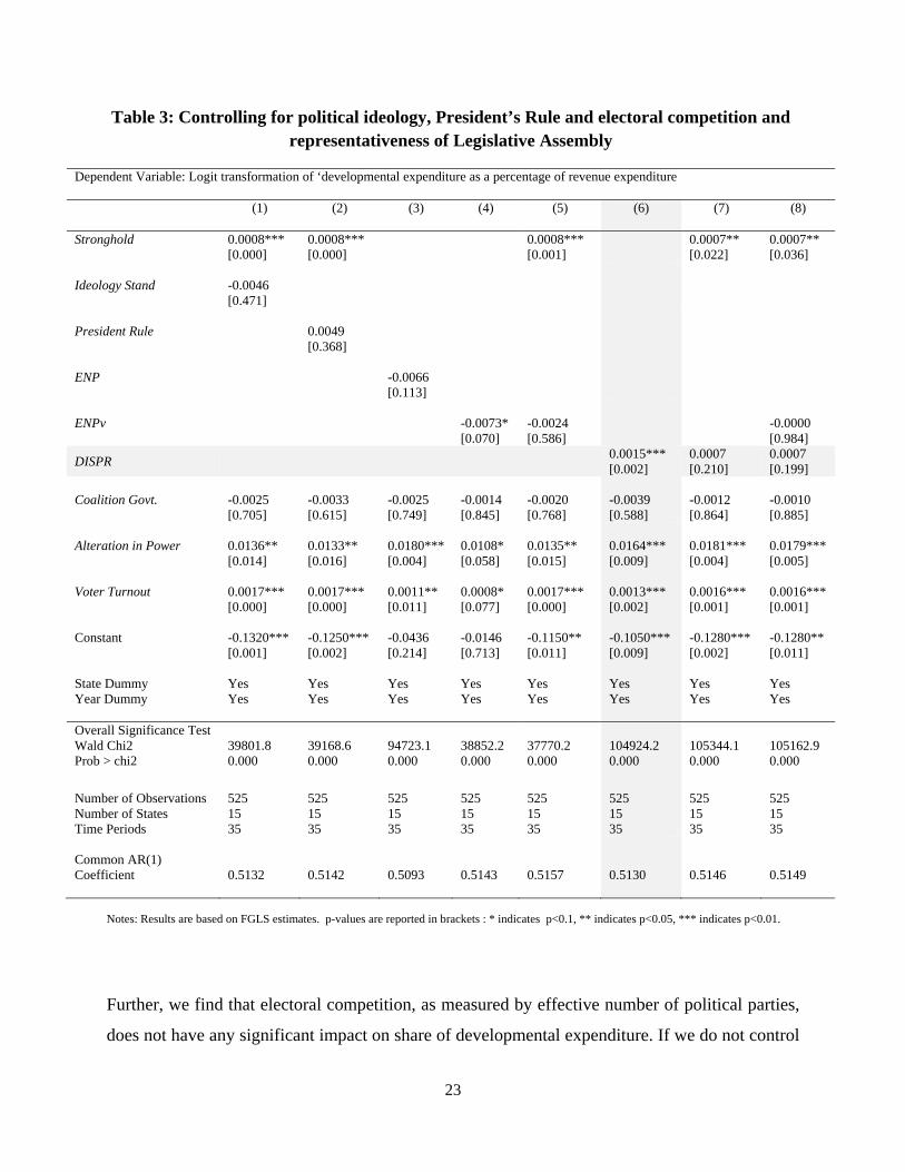
Table 3: Controlling for political ideology, President’s Rule and electoral competition and representativeness of Legislative Assembly

Dependent Variable: Logit transformation of ‘developmental expenditure as a percentage of revenue expenditure

  (1)

(2)

(3)

(4)

(5) (6) (7) (8)

Stronghold

0.0008*** [0.000]

0.0008*** [0.000]

0.0008*** [0.001]

0.0007** [0.022]

0.0007** [0.036]

Ideology Stand

-0.0046 [0.471]

President Rule

0.0049 [0.368]

ENP

-0.0066 [0.113]

ENPv

-0.0073* [0.070]

-0.0024 [0.586]

-0.0000 [0.984]

DISPR 0.0015*** [0.002]

0.0007 [0.210]

0.0007 [0.199]

Coalition Govt.

-0.0025 [0.705]

-0.0033 [0.615]

-0.0025 [0.749]

-0.0014 [0.845]

-0.0020 [0.768]

-0.0039 [0.588]

-0.0012 [0.864]

-0.0010 [0.885]

Alteration in Power

0.0136** [0.014]

0.0133** [0.016]

0.0180*** [0.004]

0.0108* [0.058]

0.0135** [0.015]

0.0164*** [0.009]

0.0181*** [0.004]

0.0179*** [0.005]

Voter Turnout

0.0017*** [0.000]

0.0017*** [0.000]

0.0011** [0.011]

0.0008* [0.077]

0.0017*** [0.000]

0.0013*** [0.002]

0.0016*** [0.001]

0.0016*** [0.001]

Constant

-0.1320*** [0.001]

-0.1250*** [0.002]

-0.0436 [0.214]

-0.0146 [0.713]

-0.1150** [0.011]

-0.1050*** [0.009]

-0.1280*** [0.002]

-0.1280** [0.011]

State Dummy Yes Yes Yes Yes Yes Yes Yes Yes

Year Dummy

Yes

Yes

Yes

Yes

Yes Yes Yes Yes

Overall Significance Test Wald Chi2 39801.8 39168.6 94723.1 38852.2 37770.2 104924.2 105344.1 105162.9 Prob > chi2

0.000

0.000

0.000

0.000

0.000 0.000 0.000 0.000

Number of Observations 525 525 525 525 525 525 525 525 Number of States Time Periods

15 35

15 35

15 35

15 35

15 35

15 35

15 35

15 35

Common AR(1) Coefficient

0.5132

0.5142

0.5093

0.5143

0.5157 0.5130

0.5146

0.5149

Notes: Results are based on FGLS estimates. p-values are reported in brackets : * indicates p<0.1, ** indicates p<0.05, *** indicates p<0.01.

Further, we find that electoral competition, as measured by effective number of political parties,

does not have any significant impact on share of developmental expenditure. If we do not control

24  

for the variable Stronghold, the coefficient of ENPv turns out to be negative and significant at

10% level, (see, Column 4 in Table 3). However, when we control for Stronghold, the coefficient

of ENPv becomes insignificant (see, Column 5 in Table 3). Therefore, it seems that ENPv is

picking up the effect of the ruling party’s political stronghold, when ENPv is considered in

isolation. The coefficient of ENP is also insignificant at 10% level (see, Column 3 in Table 4).

This result is in contrast to the conventional wisdom that electoral competition matters for

delivery of public goods (Chhibber and Nooruddin, 2004; Saez and Sinha, 2009). Also, note that

the effects of Stronghold, Alteration in Power, Voter Turnout and Coalition Govt. do not alter

irrespective of whether we control for electoral competition or not.

Finally, we turn to examine whether disproportional representation in legislative assemblies

plays any role to determine the share of developmental expenditure. We find that the coefficient

of the variable DISPR is positive and significant only if we do not control for political stronghold

of the ruling party (Stronghold), see Column 6 in Table 3. In all other cases, when we control for

electoral competition (ENPv) and/or Stronghold, the coefficient of DISPR turns out to be

insignificant (see, Column 7 and 8 in Table 3). Therefore, it appears that the extent of

representativeness of legislative assemblies does not have any significant effect on allocation of

revenue budget for developmental expenditure by the state governments. It implies that, though

greater representativeness of elected bodies is considered to be better for any democracy,

discrepancies between seat share and vote share of the political parties need not necessarily

distort the governments’ preferences for developmental expenditure over non-developmental

expenditure in case of developing countries with multiparty political system guided by majority

voting rule.

It is interesting to note that the coefficient of Stronghold remains positive and significant even if

we control for ENPv and/or DISPR. Therefore, we can say that the result of positive and

significant effect of political stronghold of the ruling party on allocation of revenue budget for

developmental expenditure in a state is robust. As mentioned before, results of this analysis do

not change if we consider alternative measures of ruling party’s stronghold and/or employ

alternative methodologies of estimation.

25  

5. Conclusion

In this paper we have examined the effects of various political factors on budget allocation

decisions of sub-national governments in India, by focusing on allocation of revenue budget for

developmental expenditure. We have constructed a measure of political stronghold of the ruling

party in a state, based on constituency level electoral outcome, to examine its impact on budget

allocation. This is perhaps the first attempt to quantify the ruling party’s political stronghold in

case of multiparty political system, using disaggregated data. We use data from 15 major states

in India during the period 1971-2005 for the purpose of the present analysis.

We find that political stronghold of the ruling party significantly affects the budget allocation

decision of the government. Greater stronghold of the ruling party in a state leads to significantly

higher proportion of revenue budget allocated for developmental expenditure. In other words,

preference of a government for developmental expenditure over non-developmental expenditure

and grants-in-aid contribution together is stronger, if the major ruling party of that government

has stronghold in larger percentage of electoral constituencies than that of other governments. It

implies that the ruling parties with lower probability to be re-elected divert funds from

developmental sectors to spend more on fiscal services, secretariat services, pensions for

government employees, etc. Econometric analysis of this paper also reveals that (a) the share of

developmental expenditure increases with the increase in proportion of politically active citizens,

which is measured by voters’ turnout, in a state and (b) change of the ruling party leads to

allocation of higher proportion of revenue budget for developmental expenditure compared to

that in case the incumbent ruling party retains the office. Our results also indicate that greater

reliance on market forces during the post economic liberalization in India has induced the state

governments to reduce the share of developmental expenditure. These are interesting results.

Moreover, we demonstrate that within government fragmentation and political ideology of the

ruling party do not have any significant effect on allocation of revenue budget for developmental

expenditure by the state governments. Effective number of political parties in a state and

representativeness of the state government also do not appear to play any role as far as the state

governments’ preferences for developmental expenditure is concerned. Our results are robust to

alternative specifications of econometric model and estimation methodologies.

26  

It is often argued that allocation of budget between capital expenditure and revenue expenditure

plays important role for economic growth (Butkiewicz and Yanikkaya, 2011; Muinelo‐Gallo and

Roca‐Sagalés, 2011; Devarajan et al., 1996). Therefore, it seems to be interesting to extend the

present analysis, in line with Uppal (2011), to examine the implications of political stronghold of

the ruling party on allocation of budget between capital expenditure and revenue expenditure. It

might also be interesting to assess the role of political factors on relative importance paid to

different social services, e.g., health, education, water supply, etc., by the governments,

particularly in the context of developing countries. However, these are beyond the scope of the

present paper. We leave these for future research.

References Alesina, A., Gerald, D. C. and Nouriel, R. (1992) “Macroeconomic policy and elections in

OECD democracies” Economics and Politics, Vol. 4(1), pp. 1-30

Arellano, M. and Bond, S. (1991) “Some tests of specification for panel data: Monte Carlo evidence and an application to employment equations” Review of Economic Studies, Vol. 58(2), pp. 277–297.

Arulampalam, W., Dasgupta, S., Dhillon, A. and Dutta, B. (2009) “Electoral goals and center-state transfers: A theoretical model and empirical evidence from India” Journal of Development Economics, Vol. 88(1), pp. 103-119.

Baltagi, B. H. (2008) Econometric analysis of panel data, 4th Edition, John Wiley, UK

Barro, R. J. (1991) “Economic growth in a cross section of countries” Quarterly Journal of Economics, Vol. 106(2), pp. 407-443

Baskaran, T. (2011) “Fiscal decentralization, ideology, and the size of the public sector” European Journal of Political Economy, Vol. 27(3), pp. 485-506

Baum, C. F. (2001) “Residual diagnostics for cross-section time series regression models” Stata Journal, Vol. 1(1), pp. 101–104

Beck, N. and Katz, J. N. (1995) “What to do (and not to do) with time-series cross-section data” American Political Science Review, Vol. 89(3), pp. 634-647

Besley, T. and Burgess, R. (2002) “The political economy of government responsiveness: theory and evidence from India” Quarterly Journal of Economics, Vol. 117(4), pp.1415–1451

27  

Blundell, R. and Bond, S. (1998) “Initial conditions and moment restrictions in dynamic panel data models” Journal of Econometrics, Vol. 87(1), pp. 115–143

Bortolotti, B. and Pinotti, P. (2008) “Delayed privatization” Public Choice, Vol. 136(3-4), pp. 331-351

Butkiewicz, J. L. and Yanikkaya, H. (2011) “Institutions and the impact of government spending on growth” Journal of Applied Economics, Vol. 14 (2), pp. 319-341

Chhibber, P. and Nooruddin, I. (2004) “Do party systems count? The number of parties and government performance in the Indian states” Comparative Political Studies, Vol. 37(2), pp.152–187

Cozzi, G. and Impullitti, G. (2010) “Government spending composition, technical change, and wage inequality” Journal of the European Economic Association, Vol. 8(6), pp. 1325-1358

Devarajan, S., Swaroop, V. and Zou, H. (1996) “The composition of public expenditure and economic growth” Journal of Monetary Economics, Vol. 37(2), pp. 313-344

Dreher, A., Sturm, J-E., and Ursprung, H. (2008) “The impact of globalization on the composition of government expenditures: Evidence from panel data” Public Choice, Vol. 134(3), pp. 263-292

Drukker, D. M. (2003) “Testing for serial correlation in linear panel-data models” Stata Journal, Vol. 3(2), pp. 168-177

Dutt, G. and Ravallion, M. (2002) “Is India’s economic growth leaving the poor behind?” Journal of Economic Perspectives, Vol.16 (3), pp. 89-108

Ferraz, C. and Finan, F. (2011) “Electoral accountability and corruption: Evidence from the audits of local governments” American Economic Review, Vol. 101(4), pp. 1274–1311

Gallagher. M. (1991) “Proportionality, disproportionality and electoral Systems” Electoral Studies, Vol. 10(1), pp.33-51

Greene W, (2003) Econometric Analysis, 5th Edition, Pearson Education, New Delhi

Gupta, S., Verhoven, M. and Tiongson, E. (2002) “The effectiveness of government spending on education and health care in developing and transition economies” European Journal of Political Economy, Vol. 18(4), pp. 717–737

Hong, H. and Ahmed, S. (2009) “Government spending on public goods: Evidence on growth and poverty” Economic and Political Weekly, Vol. 44(31), pp. 102-108

Kaushik, A. and Pal, R. (2012) “How representative has the Lok Sabha been?” Economic and Political Weekly, Vol. 47(19), pp. 74-78

28  

Khemani, S. (2004) “Political cycles in a developing economy” Journal of Development Economics, Vol. 73(1), pp. 125–154

Khemani, S. and Keefer, P. (2009) “When do legislators pass on pork? The role of political parties in determining legislator effort” American Political Science Review, Vol. 103(1), pp. 99-112

Laakso, M. and Taagepera, R. (1979) “The effective number of parties: A measure with application to West Europe” Comparative Political Studies, Vol. 12(1), pp. 3-27

Lalvani. M. (2005) “Coalition governments: Fiscal implication for the Indian economy” American Review of Political Economy, Vol. 3(1), pp. 127-163

Maddala, G. S., Li, H., Trost, R. P. and Joutz, F. (1997) “Estimation of short-run and long-run elasticities of energy demand from panel data using shrinkage estimators” Journal of Business Economics and Statistics Vol. 15(1), pp. 90-100

Muinelo‐Gallo, L. and Roca‐Sagalés, O. (2011) “Economic growth and inequality: The role of fiscal policies” Australian Economic Papers, Vol. 50(2-3), pp. 74-97

Pal, R. (2010) “Impact of communist parties on the individual decision to join a trade union: Evidence from India” The Developing Economies, Vol. 48(4), pp. 496 – 528

Potrafke, N. (2011) “Does government ideology influence budget composition? Empirical evidence from OECD countries” Economics of Governance, Vol. 12(2), pp. 101-134

Rajkumar, A. S. and Swaroop, V. (2008) “Public spending and outcomes: Does governance matter?” Journal of Development Economics, Vol. 86(1), pp. 96-111

Saez, L. and Sinha, A. (2009) “Political cycles, political institutions, and public expenditure in India, 1980-2000" British Journal of Political Science, Vol. 40(1), pp. 91-113

Uppal, Y. (2011) “Does legislative turnover adversely affect state expenditure policy? Evidence from Indian state elections” Public Choice, Vol. 147(1), pp. 189–207

29  

APPENDIX

A1 Diagnostic tests for heteroscedasticity, contemporaneous correlation and autocorrelation

Table 4: Tests for Heteroscedasticity, Contemporaneous Correlation and

Autocorrelation (1) (2) (3) (4) (5) (6) Modified Wald test for heteroscedasticity

H0: 22 σσ =n . H1:

22 σσ ≠n 2χ (15) =

Prob> 2χ =

272.92 0.0000

143.31 0.0000

355.98 0.0000

250.64 0.0000

94.79 0.0000

473.29 0.0000

Breusch-Pagan LM test for contemporaneous correlation H0: 0=njσ . H1:

0≠njσ

2χ (105) =

Prob> 2χ =

1649.727 0.0000

1051.926 0.0000

437.939 0.0000

1576.261 0.0000

1039.70 0.0000

383.452 0.0000

Wooldridge test for first order autocorrelation H0: 0=ρ . H1: 0≠ρ F( 1, 14) = Prob > F =

41.545 0.0000

42.851 0.0000

38.072 0.0000

41.545 0.0000

42.851 0.0000

38.072 0.0000

Notes: Test results in column (1) corresponds to the base-line regression of Model 1 with the explanatory variables

Stronghold, Coalition Govt., Alteration in Power and Voter Turnout. Base-line regression corresponding to column (2)

includes Liberalisation Dummy as an additional explanatory variable. Next, we drop Liberalisation Dummy and introduce

Year Dummies in the base-line regression for column (3). Then we drop Year Dummies and introduce State Dummies for

the base line regression corresponding to column 4. In base-line regression corresponding to column (5) we introduce

Liberalisation Dummy along with State Dummies. Finally, we drop Liberalisation Dummy and introduce Year Dummies

along with State Dummies to perform the baseline regression for results in column (6).

Modified Wald test is a Chi-square test for group wise heteroscedasticity, which tests the null hypothesis of a common

variance 22 σσ =n against the alternative of group wise heteroscedasticity, where the test statistic is )(2 Nχ

distributed. The Breusch-Pagan LM test of cross-sectional independence is based on the average of the squared pair-wise

correlation coefficients of the residuals and is applicable in the case of temporally dominant (i.e., NT > ) panel data

models where the cross section dimension (N) is small relative to the time dimension (T). Under the null hypothesis

);,....,2,1,(0 jnNjnnj ≠=∀=σ , the LM statistic is )

2)1((2 −NNχ

distributed. See Greene (2003) and

Baum (2001) for details. In Wooldridge test for autocorrelation in panel data the test statistic is based on heteroscedasticity

and autocorrelation consistent (HAC) standard errors, which makes the test robust against cross-sectional heteroscedasticity.

Under the null hypothesis of no first order autocorrelation, the test statistic follows F(1, T-1)-distribution. See Woodlridge

(2002) and Drukker (2003) for details.

30  

A2 Beck-Katz estimates with panel corrected Standard Errors

Table 5: Electoral stronghold of ruling party and developmental expenditure – Beck-Katz estimates with panel corrected Standard Errors

Dependent Variable: Logit transformation of ‘developmental expenditure as a percentage of revenue expenditure

(1) (2) (3) (4) (5) (6)

Stronghold

0.0022*** [0.000]

0.0022*** [0.000]

0.0012*** [0.001]

0.0022*** [0.000]

0.0020*** [0.000]

0.0015*** [0.000]

Coalition Govt.

-0.0154 [0.222]

-0.0197 [0.106]

-0.0112 [0.300]

-0.0147 [0.258]

-0.0167 [0.194]

-0.0094 [0.421]

Alteration in Power

0.0274** [0.017]

0.0312*** [0.010]

0.0120 [0.164]

0.0272** [0.020]

0.0368*** [0.003]

0.0054 [0.533]

Voter Turnout

0.0017** [0.042]

0.0016** [0.044]

0.0017*** [0.008]

0.0016* [0.068]

0.0014 [0.135]

0.0017** [0.050]

Liberalisation Dummy

-0.0904*** [0.006]

-0.116*** [0.000]

Constant

0.0615 [0.373]

0.124** [0.038]

-0.0564 [0.235]

-0.0031 [0.971]

0.0972 [0.226]

0.0030 [0.970]

State Dummies No No No Yes Yes

Yes

Year Dummies

No

No

Yes

No

No

Yes

R- Squared

0.0670

0.1300

0.4660

0.0842

0.2310

0.2541

Overall Significance Test: Wald Chi2 29.44 43.49 4606.9 99.64 296.9

152.77

Prob > chi2

0.000

0.000

0.000

0.000

0.000

0.000

Number of Observations 525 525 525 525 525

525

Number of States Time Periods

15 35

15 35

15 35

15 35

15 35

15 35

Common AR(1) Coefficient

0.8307

0.6849

0.6796

0.8088

0.6100

0.7794

Notes: p-values are reported in brackets : * indicates p<0.1, ** indicates p<0.05, *** indicates p<0.01.

A3 Robustness Analysis with alternative measures of stronghold

As mentioned before, we do some robustness checks using alternative measures of political

stronghold of the ruling party. We study four different measures of political stronghold. We

change the critical value of “Vote share of winner*Margin of win” from the average value to

105% and 110% of average value, and denote the new variables by SW2 and SW3, respectively.

Other than these two measures, we also consider the average winning margin (SM1) and 110% of

average winning margin (SM2) as alternative measures of political stronghold of the ruling party.

31  

Table 6: Robustness analysis using alternative measures of electoral Stronghold Dependent Variable: Logit transformation of ‘developmental expenditure as a percentage of revenue expenditure

(1) (2) (3) (4)

SW2

0.0009*** [0.000]

SW3

0.0009*** [0.000]

SM1

0.0009*** [0.001]

SM2

0.0009*** [0.000]

Coalition Govt.

-0.0018 [0.800]

-0.0015 [0.832]

-0.0007 [0.922]

-0.0022 [0.742]

Alteration in Power

0.0191*** [0.002]

0.0192*** [0.002]

0.0181*** [0.004]

0.0126** [0.023]

Voter Turnout

0.0015*** [0.001]

0.0016*** [0.001]

0.0015*** [0.001]

0.0018*** [0.000]

Constant

-0.1150*** [0.005]

-0.1180*** [0.004]

-0.1130*** [0.006]

-0.1310*** [0.001]

State Dummies Yes Yes Yes Yes

Year Dummies

Yes

Yes

Yes

Yes

Overall Significance Test: Wald Chi2 101996.0 101396.0 102968.4 38222.7 Prob > chi2

0.000

0.000

0.000

0.000

Number of Observations 525 525 525 525 Number of States Time Periods

15 35

15 35

15 35

15 35

Common AR(1) Coefficient

0.5167

0.5162

0.5138

0.5145

Notes: Results are based on FGLS estimates. p-values are reported in brackets : * indicates p<0.1, ** indicates p<0.05, *** indicates p<0.01.

Table 6 presents the results of FGLS estimation corresponding to alternative measures of

Stronghold. Clearly, our results are not sensitive to alternative measures of Stronghold (see Table

2 and Table 6). We also compute the Beck-Katz estimates with panel corrected Standard Errors to

check the robustness of our results with alternative measures of Stronghold and estimation method, which

we present in Table 7. It is evident that our results are robust to alternative methodology of estimation as

well.

32  

Table 7: Robustness analysis using alternative measures of electoral Stronghold - Beck-Katz estimates with panel corrected Standard Errors

Dependent Variable: Logit transformation of ‘developmental expenditure as a percentage of revenue expenditure

(1) (2) (3) (4)

SW2

0.0009** [0.021]

SW3

0.0009** [0.024]

SM1

0.0008** [0.042]

SM2

0.0008** [0.044]

Coalition Govt.

-0.0075 [0.486]

-0.0073 [0.498]

-0.0063 [0.563]

-0.0068 [0.533]

Alteration in Power

0.0178** [0.019]

0.0179** [0.019]

0.0171** [0.025]

0.0171** [0.026]

Voter Turnout

0.0019** [0.011]

0.0019** [0.011]

0.0018** [0.014]

0.0019** [0.013]

Constant

-0.1320**

[0.035] -0.1330**

[0.035] -0.1280**

[0.043] -0.1290**

[0.044] State Dummies Yes Yes Yes Yes Year Dummies

Yes

Yes

Yes

Yes

R- Squared 0.611 0.612 0.612 0.612 Overall Significance Test: Wald Chi2 12512.0 1.11814e+15 1560.7

1.45E+15

Prob > chi2

0.000

0.000

0.000

0.000

Number of Observations 525 525 525 525 Number of States Time Periods

15 35

15 35

15 35

15 35

Common AR(1) Coefficient 0.5376 0.5371

0.5350

0.5356

Notes: p-values are reported in brackets : * indicates p<0.1, ** indicates p<0.05, *** indicates p<0.01.

 

A4 A Further Robustness Check: Exclusion of Emergency period

One may suspect that the results might change, if we exclude the period of emergency in India

from our study. Note that, during the period of emergency in India (1975-1977), all states were

under the President’s Rule simultaneously. Therefore, we re-estimate the model by considering

only the post emergency period (1978-2005), results of which are reported in Table 8.

33  

Table 8: Estimates for post emergency period: 1978-2005 (Robustness Check)

Dependent Variable: Logit transformation of ‘developmental expenditure as a percentage of revenue expenditure (1)  (2) 

Stronghold

0.0010*** [0.001]

0.0005* [0.061]

ENPV

-0.0022 [0.640]

DISPR

0.0009* [0.096]

Coalition Govt.

-0.0058 [0.469]

-0.0062 [0.381]

Alteration in Power

0.0126* [0.079]

0.0074 [0.219]

Voter Turnout

0.0014*** [0.005]

0.0016*** [0.001]

Constant

-0.0957** [0.042]

-0.1070** [0.023]

State Dummies Yes Yes

Year Dummies

Yes

Yes

Overall Significance Test: Wald Chi2 150955.4 47727.8 Prob > chi2

0.000

0.000

Number of Observations 420 420 Number of States Time Periods

15 28

15 28

Common AR(1) Coefficient 0.4751 0.4722 Notes: Results are based on FGLS estimates. p-values are reported in brackets : * indicates p<0.1, ** indicates p<0.05, *** indicates p<0.01.

 

***