Pole-Placement Design – A State-Space Approach · Pole-Placement Design – A State-Space...

TU Berlin Discrete-Time Control Systems 1

Pole-Placement Design – A State-Space Approach

Overview

• Control-System Design

• Regulation by State Feedback

• Observers

• Output Feedback

• The Servo Problem

11th July 2013


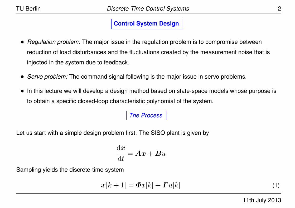
Control System Design

• Regulation problem: The major issue in the regulation problem is to compromise between

reduction of load disturbances and the fluctuations created by the measurement noise that is

injected in the system due to feedback.

• Servo problem: The command signal following is the major issue in servo problems.

• In this lecture we will develop a design method based on state-space models whose purpose is

to obtain a specific closed-loop characteristic polynomial of the system.

The Process

Let us start with a simple design problem first. The SISO plant is given by

dx

dt= Ax+Bu

Sampling yields the discrete-time system

x[k + 1] = Φx[k] + Γu[k] (1)

11th July 2013


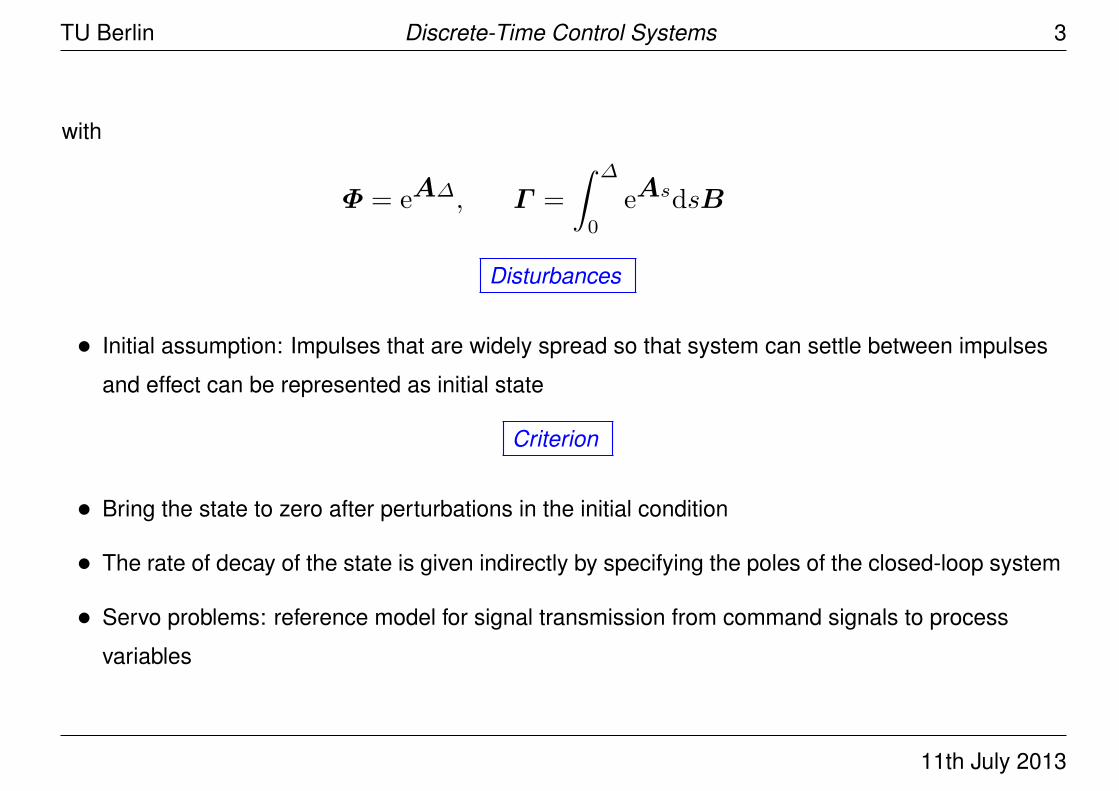
with

Φ = eA∆, Γ =

∫ ∆

0

eAsdsB

Disturbances

• Initial assumption: Impulses that are widely spread so that system can settle between impulses

and effect can be represented as initial state

Criterion

• Bring the state to zero after perturbations in the initial condition

• The rate of decay of the state is given indirectly by specifying the poles of the closed-loop system

• Servo problems: reference model for signal transmission from command signals to process

variables

11th July 2013


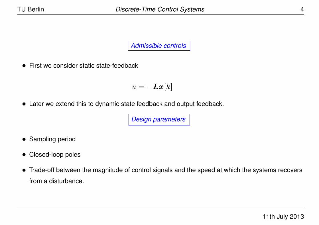
Admissible controls

• First we consider static state-feedback

u = −Lx[k]

• Later we extend this to dynamic state feedback and output feedback.

Design parameters

• Sampling period

• Closed-loop poles

• Trade-off between the magnitude of control signals and the speed at which the systems recovers

from a disturbance.

11th July 2013


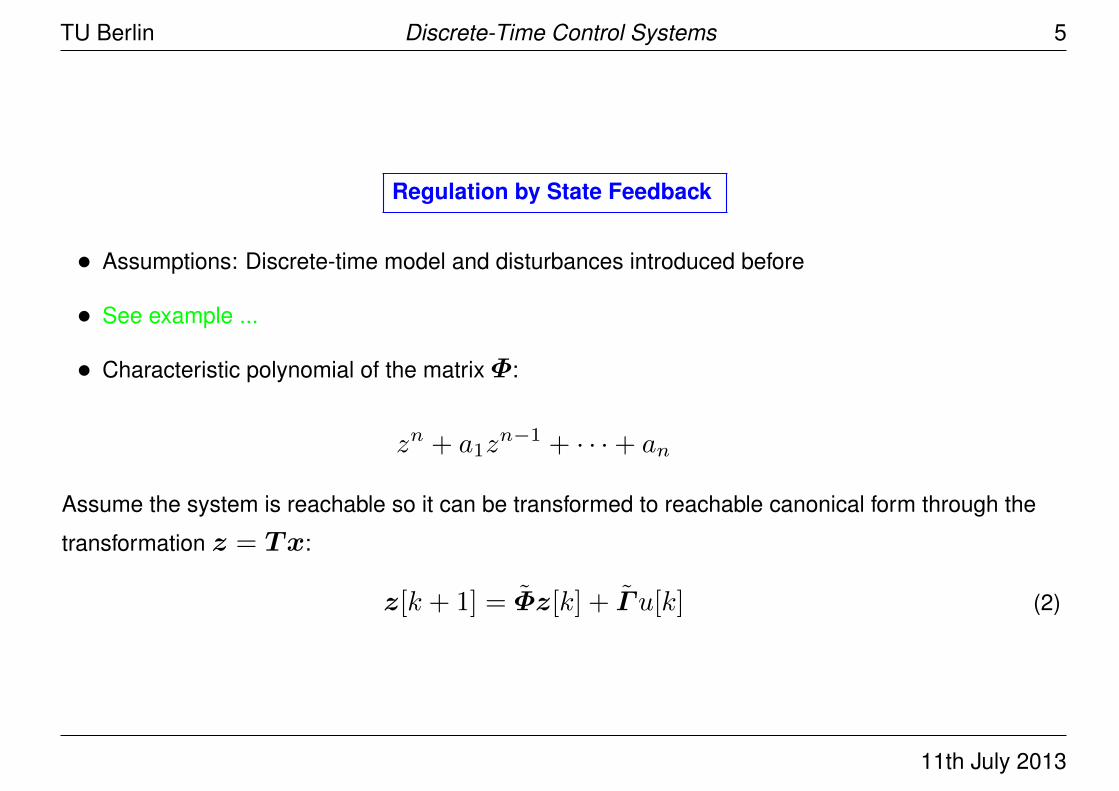
Regulation by State Feedback

• Assumptions: Discrete-time model and disturbances introduced before

• See example ...

• Characteristic polynomial of the matrixΦ:

zn + a1zn−1 + · · ·+ an

Assume the system is reachable so it can be transformed to reachable canonical form through the

transformation z = Tx:

z[k + 1] = Φz[k] + Γu[k] (2)

11th July 2013


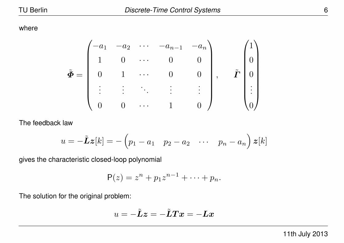
where

Φ =

−a1 −a2 · · · −an−1 −an1 0 · · · 0 0

0 1 · · · 0 0...

.... . .

......

0 0 · · · 1 0

, Γ

1

0

0...

0

The feedback law

u = −Lz[k] = −(p1 − a1 p2 − a2 · · · pn − an

)z[k]

gives the characteristic closed-loop polynomial

P(z) = zn + p1zn−1 + · · ·+ pn.

The solution for the original problem:

u = −Lz = −LTx = −Lx

11th July 2013


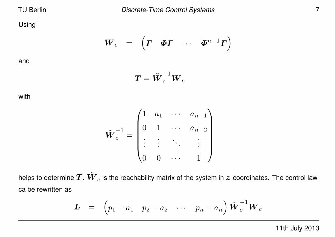
Using

W c =(Γ ΦΓ · · · Φn−1Γ

)and

T = W−1

c W c

with

W−1

c =

1 a1 · · · an−1

0 1 · · · an−2

......

. . ....

0 0 · · · 1

helps to determine T . W c is the reachability matrix of the system in z-coordinates. The control law

ca be rewritten as

L =(p1 − a1 p2 − a2 · · · pn − an

)W

−1

c W c

11th July 2013


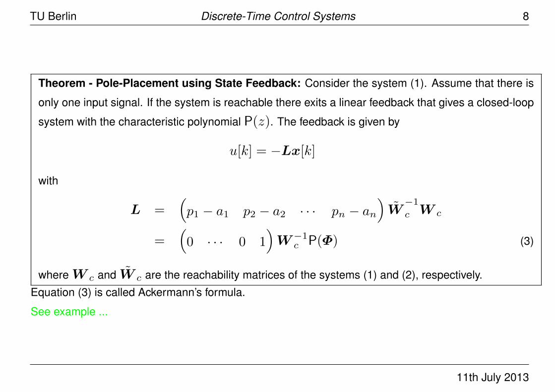
Theorem - Pole-Placement using State Feedback: Consider the system (1). Assume that there is

only one input signal. If the system is reachable there exits a linear feedback that gives a closed-loop

system with the characteristic polynomial P(z). The feedback is given by

u[k] = −Lx[k]

with

L =(p1 − a1 p2 − a2 · · · pn − an

)W

−1

c W c

=(0 · · · 0 1

)W−1

c P(Φ) (3)

whereW c and W c are the reachability matrices of the systems (1) and (2), respectively.

Equation (3) is called Ackermann’s formula.

See example ...

11th July 2013


Deadbeat Control

If the desired poles are all chosen to be at the origin, the characteristic polynomial of the closed-loop

system becomes

P(z) = zn.

The system matrix of the closed-loop system satisfies

Φnc = Φ− ΓL = 0

• This strategy has the property that it will drive all states to zero in at most n steps after an

impulse disturbance in the system state.

• The control strategy is called deadbeat control.

• There is only one design parameter – the sampling period.

• The settling time is given by n ·∆.

11th July 2013


Taking into account disturbances

• In order to handle more general disturbances than impulse we assume

dx

dt= Ax+Bu+ v

where v is a disturbance described by

dw

dt= Aww

v = Cww

with given initial conditions.

• Aw = 0: disturbance v is a constant.

• Aw =

0 ω0

−ω0 0

: sinusoidal disturbance

• It is assumed thatw can be measured. This assumption is relaxed later.

11th July 2013


Augmented state vector:

z =

xw

Complete system:

d

dt

xw

=

A Cω

0 Aw

xw

+

B0

u

After sampling: x[k + 1]

w[k + 1]

=

Φ Φxw

0 Φw

x[k]w[k]

+

Γ0

u[k]

General linear state feedback:

u[k] = −Lx[k]−Lww[k] (4)

11th July 2013


Resulting closed-loop system:

x[k + 1] = (Φ− ΓL)x[k] + (Φxw − ΓLw)w[k]

w[k + 1] = Φww[k]

• Combination of a feedback term Lx and a feedforward term Lww

• If the pair (Φ,Γ ) is reachable, the matrix L can be chosen so that the matrix (Φ− ΓL) has

prescribed eigenvalues.

• The matrixΦw can not be influenced by feedback.

• By proper choice of Lw , the influence of disturbances on the state vector x can be made small.

• Select Lw that makes (Φxw − ΓLw) small or even zero.

See example ...

11th July 2013


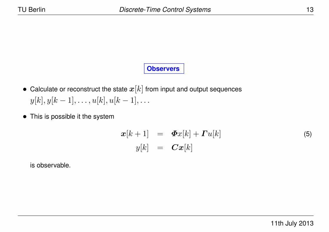
Observers

• Calculate or reconstruct the state x[k] from input and output sequences

y[k], y[k − 1], . . . , u[k], u[k − 1], . . .

• This is possible it the system

x[k + 1] = Φx[k] + Γu[k] (5)

y[k] = Cx[k]

is observable.

11th July 2013


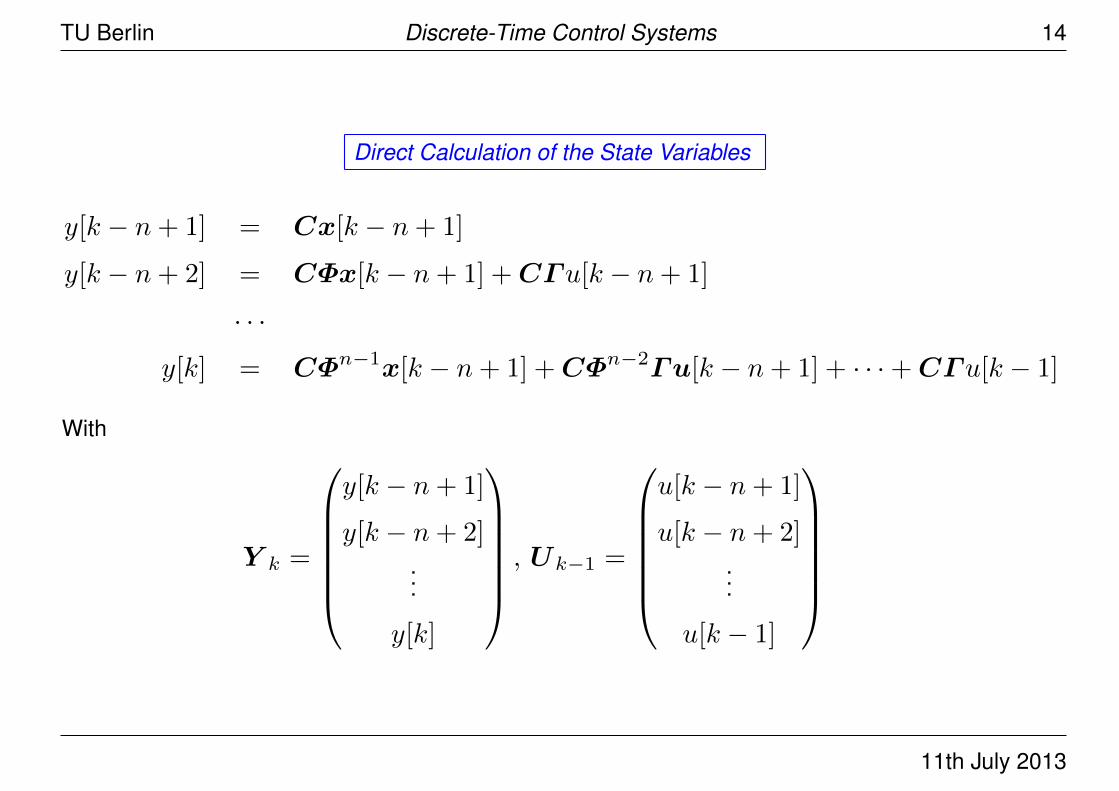
Direct Calculation of the State Variables

y[k − n+ 1] = Cx[k − n+ 1]

y[k − n+ 2] = CΦx[k − n+ 1] +CΓu[k − n+ 1]

· · ·

y[k] = CΦn−1x[k − n+ 1] +CΦn−2Γu[k − n+ 1] + · · ·+CΓu[k − 1]

With

Y k =

y[k − n+ 1]

y[k − n+ 2]...

y[k]

, Uk−1 =

u[k − n+ 1]

u[k − n+ 2]...

u[k − 1]

11th July 2013


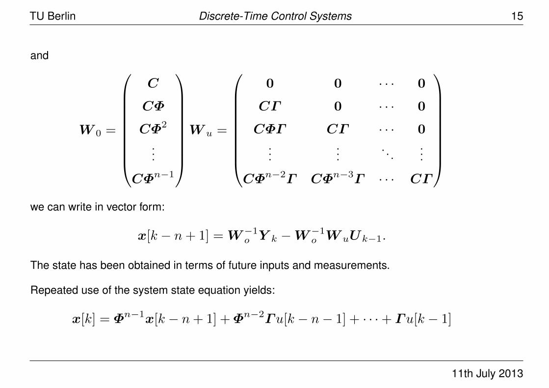
and

W 0 =

C

CΦ

CΦ2

...

CΦn−1

W u =

0 0 · · · 0

CΓ 0 · · · 0

CΦΓ CΓ · · · 0...

.... . .

...

CΦn−2Γ CΦn−3Γ · · · CΓ

we can write in vector form:

x[k − n+ 1] =W−1o Y k −W−1

o W uUk−1.

The state has been obtained in terms of future inputs and measurements.

Repeated use of the system state equation yields:

x[k] = Φn−1x[k − n+ 1] +Φn−2Γu[k − n− 1] + · · ·+ Γu[k − 1]

11th July 2013


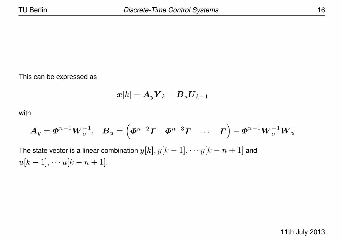
This can be expressed as

x[k] = AyY k +BuUk−1

with

Ay = Φn−1W−1o , Bu =

(Φn−2Γ Φn−3Γ · · · Γ

)−Φn−1W−1

o W u

The state vector is a linear combination y[k], y[k − 1], · · · y[k − n+ 1] and

u[k − 1], · · ·u[k − n+ 1].

11th July 2013


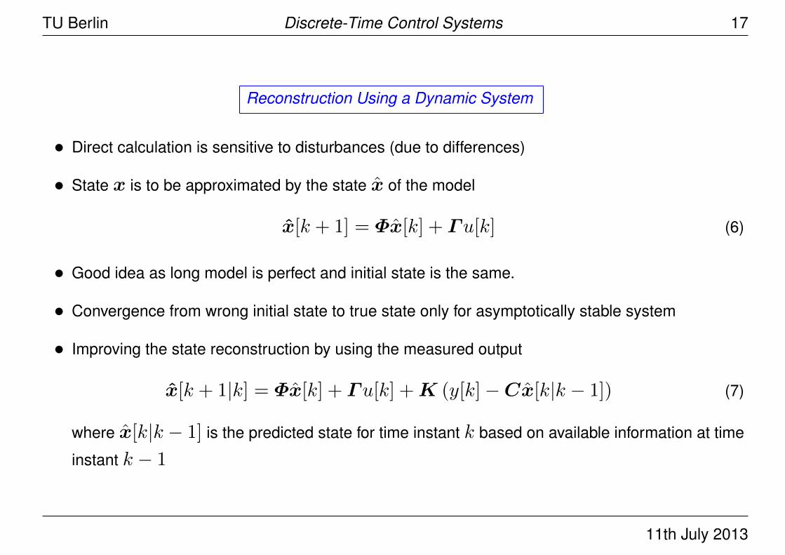
Reconstruction Using a Dynamic System

• Direct calculation is sensitive to disturbances (due to differences)

• State x is to be approximated by the state x of the model

x[k + 1] = Φx[k] + Γu[k] (6)

• Good idea as long model is perfect and initial state is the same.

• Convergence from wrong initial state to true state only for asymptotically stable system

• Improving the state reconstruction by using the measured output

x[k + 1|k] = Φx[k] + Γu[k] +K (y[k]−Cx[k|k − 1]) (7)

where x[k|k − 1] is the predicted state for time instant k based on available information at time

instant k − 1

11th July 2013


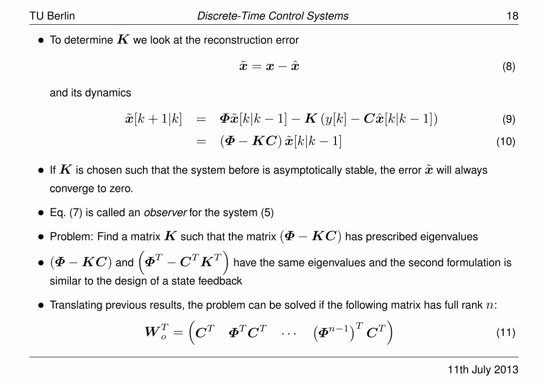
• To determineK we look at the reconstruction error

x = x− x (8)

and its dynamics

x[k + 1|k] = Φx[k|k − 1]−K (y[k]−Cx[k|k − 1]) (9)

= (Φ−KC) x[k|k − 1] (10)

• IfK is chosen such that the system before is asymptotically stable, the error x will always

converge to zero.

• Eq. (7) is called an observer for the system (5)

• Problem: Find a matrixK such that the matrix (Φ−KC) has prescribed eigenvalues

• (Φ−KC) and(ΦT −CTKT

)have the same eigenvalues and the second formulation is

similar to the design of a state feedback

• Translating previous results, the problem can be solved if the following matrix has full rank n:

W To =

(CT ΦTCT · · ·

(Φn−1

)TCT)

(11)

11th July 2013


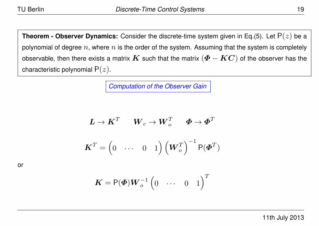
Theorem - Observer Dynamics: Consider the discrete-time system given in Eq.(5). Let P(z) be a

polynomial of degree n, where n is the order of the system. Assuming that the system is completely

observable, then there exists a matrix K such that the matrix (Φ−KC) of the observer has the

characteristic polynomial P(z).

Computation of the Observer Gain

L→KT W c →W To Φ→ ΦT

KT =(0 · · · 0 1

)(W T

o

)−1

P(ΦT )

or

K = P(Φ)W−1o

(0 · · · 0 1

)T

11th July 2013


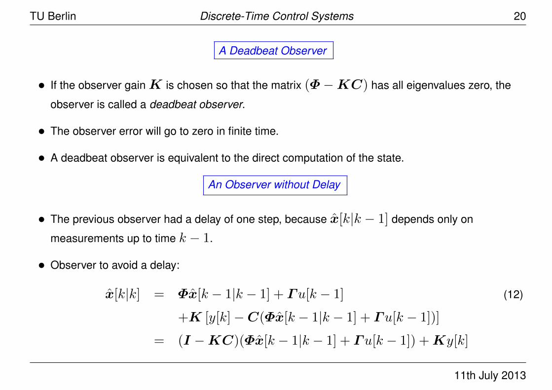
A Deadbeat Observer

• If the observer gainK is chosen so that the matrix (Φ−KC) has all eigenvalues zero, the

observer is called a deadbeat observer.

• The observer error will go to zero in finite time.

• A deadbeat observer is equivalent to the direct computation of the state.

An Observer without Delay

• The previous observer had a delay of one step, because x[k|k − 1] depends only on

measurements up to time k − 1.

• Observer to avoid a delay:

x[k|k] = Φx[k − 1|k − 1] + Γu[k − 1] (12)

+K [y[k]−C(Φx[k − 1|k − 1] + Γu[k − 1])]

= (I −KC)(Φx[k − 1|k − 1] + Γu[k − 1]) +Ky[k]

11th July 2013


• Observer error

x[k|k] = x[k]− x[k|k] = (Φ−KCΦ)x[k − 1|k − 1] (13)

• The pair (Φ,CΦ) is observable if the pair (Φ,C) is observable! This implies that arbitary

eigenvalues can be given to (Φ,CΦ) by selectionK .

y(k)−Cx[k|k] = Cx[k|k] = (I −CK)CΦx[k − 1|k − 1] (14)

• If the system has one output, then (I −CK) is a scalar. K may be chosen such that

CK = 1. This implies that y(k) = Cx[k|k]. This will make it possible to eliminate one

equation from (12). Reduced-order observes of this type are called Luenberger observers.

11th July 2013


Output Feedback

• Before it was assumed that all states are measurable.

• Now we combine the state feedback with the observer to deal with non-measurable but

observable states.

• System:

x[k + 1] = Φx[k] + Γu[k] (15)

y[k] = Cx[k]

• Aim: linear feedback law relating u to y such that the closed-loop system has given poles

• Initial assumption: impulse-like disturbances or equivalently unknown initial state

11th July 2013


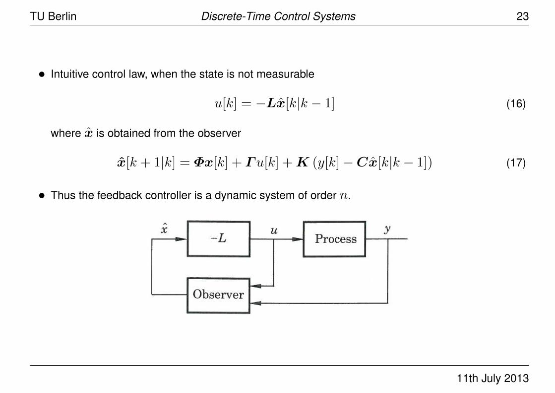
• Intuitive control law, when the state is not measurable

u[k] = −Lx[k|k − 1] (16)

where x is obtained from the observer

x[k + 1|k] = Φx[k] + Γu[k] +K (y[k]−Cx[k|k − 1]) (17)

• Thus the feedback controller is a dynamic system of order n.

11th July 2013


Analysis of the Closed-Loop System

Using

x = x− x (18)

and inserting the last control law into the considered system yields

x[k + 1] = (Φ− ΓL)x[k] + ΓLx[k|k − 1] (19)

x[k + 1|k] = (Φ−KC)x[k|k − 1] (20)

• The closed-loop system has the order 2n.

• The eigenvalues of the closed-loop system are the eigenvalues of the matrices (Φ− ΓL) and

(Φ−KC).

• Design of state feedback and observer can be separated (separation principle)

• The controller can be expressed as n-th-order pulse-transfer function from y to u:

Hc(z) = −L(zI −Φ+ ΓL)−1K (21)

11th July 2013


Output feedback without time-delay

• Use of the feedback law

u[k] = −Lx[k|k] (22)

together with the observer (12).

• The resulting closed-loop system has similar properties compared to the case before.

11th July 2013


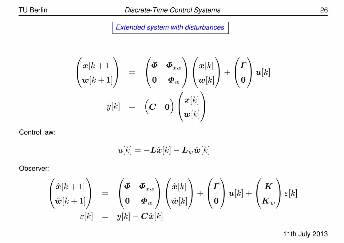
Extended system with disturbances

x[k + 1]

w[k + 1]

=

Φ Φxw

0 Φw

x[k]w[k]

+

Γ0

u[k]y[k] =

(C 0

)x[k]w[k]

Control law:

u[k] = −Lx[k]−Lww[k]

Observer: x[k + 1]

w[k + 1]

=

Φ Φxw

0 Φw

x[k]w[k]

+

Γ0

u[k] + K

Kw

ε[k]

ε[k] = y[k]−Cx[k]

11th July 2013


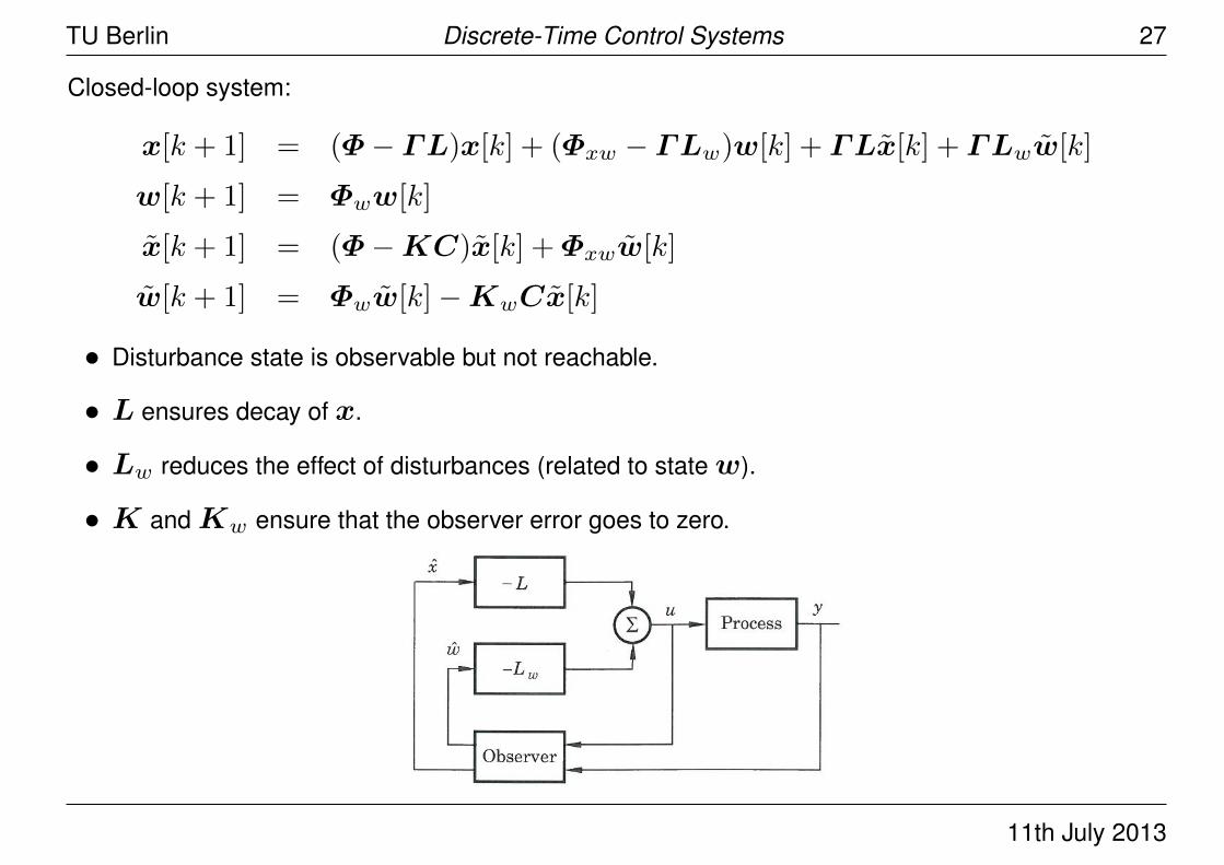
Closed-loop system:

x[k + 1] = (Φ− ΓL)x[k] + (Φxw − ΓLw)w[k] + ΓLx[k] + ΓLww[k]

w[k + 1] = Φww[k]

x[k + 1] = (Φ−KC)x[k] +Φxww[k]

w[k + 1] = Φww[k]−KwCx[k]

• Disturbance state is observable but not reachable.

• L ensures decay of x.

• Lw reduces the effect of disturbances (related to statew).

• K andKw ensure that the observer error goes to zero.

11th July 2013


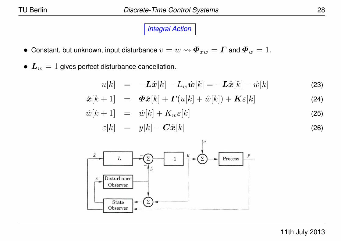
Integral Action

• Constant, but unknown, input disturbance v = w Φxw = Γ andΦw = 1.

• Lw = 1 gives perfect disturbance cancellation.

u[k] = −Lx[k]− Lww[k] = −Lx[k]− w[k] (23)

x[k + 1] = Φx[k] + Γ (u[k] + w[k]) +Kε[k] (24)

w[k + 1] = w[k] +Kwε[k] (25)

ε[k] = y[k]−Cx[k] (26)

11th July 2013


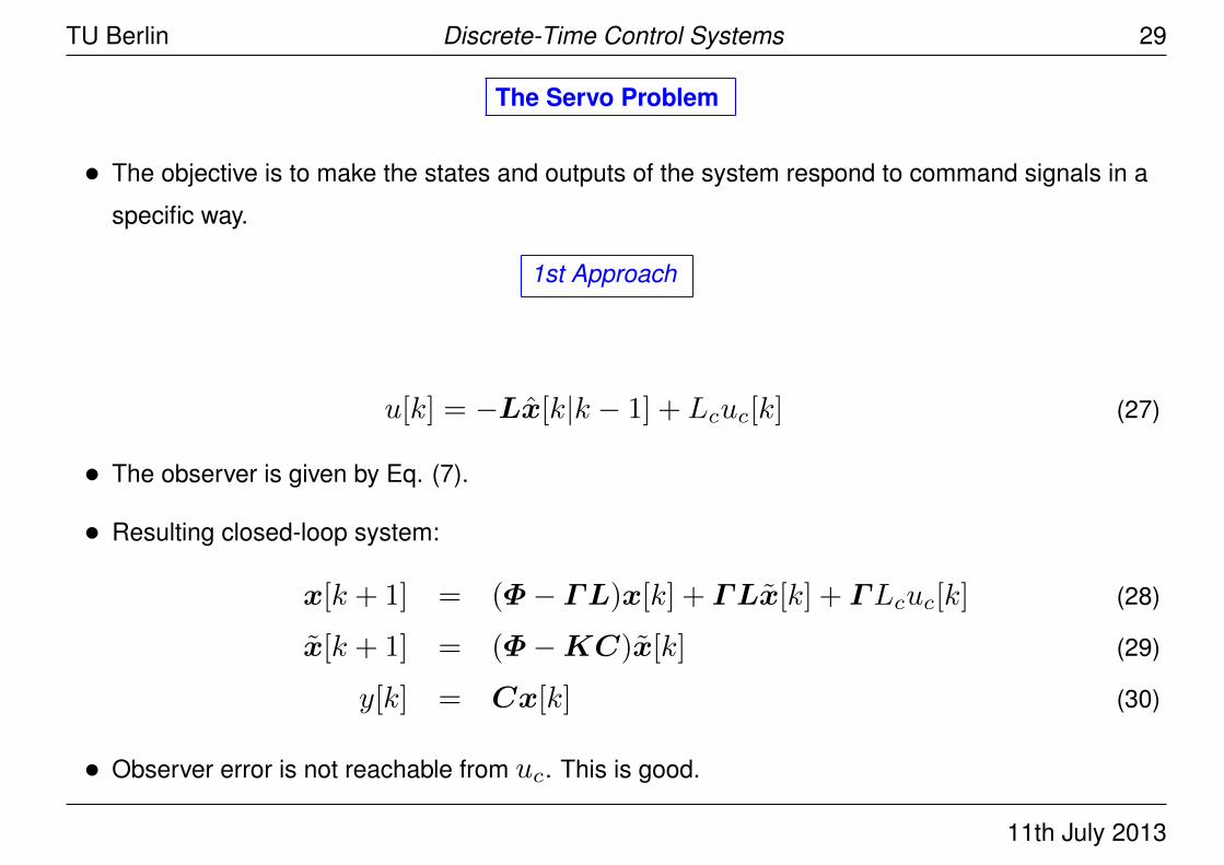
The Servo Problem

• The objective is to make the states and outputs of the system respond to command signals in a

specific way.

1st Approach

u[k] = −Lx[k|k − 1] + Lcuc[k] (27)

• The observer is given by Eq. (7).

• Resulting closed-loop system:

x[k + 1] = (Φ− ΓL)x[k] + ΓLx[k] + ΓLcuc[k] (28)

x[k + 1] = (Φ−KC)x[k] (29)

y[k] = Cx[k] (30)

• Observer error is not reachable from uc. This is good.

11th July 2013


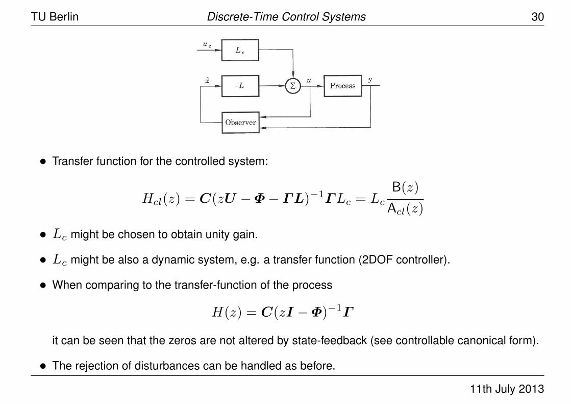
• Transfer function for the controlled system:

Hcl(z) = C(zU −Φ− ΓL)−1ΓLc = LcB(z)

Acl(z)

• Lc might be chosen to obtain unity gain.

• Lc might be also a dynamic system, e.g. a transfer function (2DOF controller).

• When comparing to the transfer-function of the process

H(z) = C(zI −Φ)−1Γ

it can be seen that the zeros are not altered by state-feedback (see controllable canonical form).

• The rejection of disturbances can be handled as before.

11th July 2013


2nd Approach

• Reference model:

xm[k + 1] = Φmxm[k] + Γmuc[k]

ym[k] = Cmxm[k]

• Control law:

u[k] = L(xm[k]− x[k|k − 1]) + uff [k] (31)

• xm[k]: desired state (coordinate systems must be compatible)

• uff : control signal that gives desired output when applied to the open-loop system.

• feedback: L(xm[k]− x[k|k − 1]), feedforward signal: uff

• Generation of the feedforward signal:

uff [k] =Hm(q)

H(q)uc[k]

11th July 2013


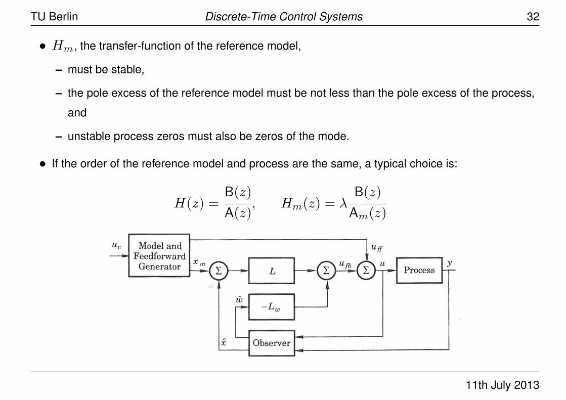
• Hm, the transfer-function of the reference model,

– must be stable,

– the pole excess of the reference model must be not less than the pole excess of the process,

and

– unstable process zeros must also be zeros of the mode.

• If the order of the reference model and process are the same, a typical choice is:

H(z) =B(z)

A(z), Hm(z) = λ

B(z)

Am(z)

11th July 2013

Pole-Placement Design – A State-Space Approach · Pole-Placement Design – A State-Space...

Documents

Transcript of Pole-Placement Design – A State-Space Approach · Pole-Placement Design – A State-Space...