PLGC II Manual - Board Rev 1b
113
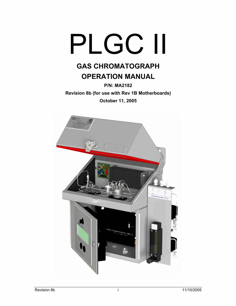
Revision 8b i 11/10/2005 PLGC II GAS CHROMATOGRAPH OPERATION MANUAL P/N: MA2182 Revision 8b (for use with Rev 1B Motherboards) October 11, 2005
-
Upload
eka-pramudia-santoso -
Category
Documents
-
view
130 -
download
37
description
PLGC II Manual - Board Rev 1b
Transcript of PLGC II Manual - Board Rev 1b
Revision 8b i 11/10/2005
PLGC II GAS CHROMATOGRAPH
OPERATION MANUAL P/N: MA2182
Revision 8b (for use with Rev 1B Motherboards) October 11, 2005

ii
Galvanic Applied Sciences, Inc.
7000 Fisher Road S.E. Calgary, Alberta, Canada
T2H 0W3 Phone: (403) 252-8470
Fax: (403) 255-6287 E-mail: [email protected]
World Wide Web: http://www.galvanic.com
Revision 8b iii 11/10/2005
Table of Contents MANUFACTURER’S WARRANTY STATEMENT ........................................ vi
Section 1 ...........................................................................................................1-1 1 Analyzer General Description..................................................................1-1
1.1 Introduction ......................................................................................1-1 1.2 Note on Theory of Operation............................................................1-1
Section 2 ...........................................................................................................2-3 2 Analyzer Component Description............................................................2-3
2.1 Standard 12-minute Cycle Time ...........................................................2-4 2.2 Detector ...........................................................................................2-7 2.3 Microprocessor Control System .......................................................2-7
Section 3 ...........................................................................................................3-9 3 Analyzer Installation and Considerations ................................................3-9
3.1 Sampling Point Location ..................................................................3-9 3.2 Sample Volume and Flow Rate........................................................3-9 3.3 Sample Conditioning ........................................................................3-9 3.4 Battery ...............................................................................................3-9 3.5 Installation........................................................................................3-9
Section 4 .........................................................................................................4-13 4 Electrical Connections and Considerations...........................................4-13
4.1 Functions of Electrical Ports...........................................................4-13 4.2 Modbus Communication ................................................................4-18 4.3 PLGC II Wiring Schedule ...............................................................4-21 4.4 PLGC II Wiring Diagrams...............................................................4-22
Section 5 .........................................................................................................5-25 5 Software Operation ...............................................................................5-25
5.1 Software Installation and Connection.............................................5-25 5.2 Interface and Icons ........................................................................5-26 5.3 Database and Devices ...................................................................5-30 5.4 Data Observation Applications.......................................................5-34 5.5 Setup Applications .........................................................................5-49 5.6 Advanced Operations.....................................................................5-75
Section 6 .........................................................................................................6-83 6 Maintenance..........................................................................................6-83
6.1 Weekly Checkup ............................................................................6-83 6.2 Gas Cylinder Replacement ............................................................6-84 6.3 Cleaning the PLGC II .....................................................................6-84 6.4 Chromatograph Valve ....................................................................6-84 6.5 Flow Control...................................................................................6-85 6.6 Column Oven .................................................................................6-86 6.7 PLGC II Parts List ..........................................................................6-86 6.8 Weekly Check-up Report ...............................................................6-87
Section 7 .........................................................................................................7-89 7 Troubleshooting ....................................................................................7-89
Section 8 .........................................................................................................8-91 Appendix A: Theory of Gas Chromatography...............................................8-91
iv
What is Gas Chromatography?.................................................................8-91 Basic Parts and Terminology of a Gas Chromatograph............................8-91 How are the components separated? .......................................................8-92 How are the Components Detected and Quantified?................................8-92 The Chromatograph Output: The Chromatogram.....................................8-93
Section 9 .........................................................................................................9-95 Appendix B: Definitions and Formulas .........................................................9-95
Definition of Terms....................................................................................9-95 Calibration Formulas and Analyzer Calculations ......................................9-96
Section 10 .....................................................................................................10-99 Appendix C: Typical Parameters of Natural Gas Components...................10-99
GPA Parameters.....................................................................................10-99 AGA Parameters...................................................................................10-100
Section 11 ...................................................................................................11-101 Appendix D: Valco 6 and 10 Port Valve Technical Information ................11-101
Valve Operation Instructions.................................................................11-101 Valve Maintenance Instructions ............................................................11-103
Section 12 ...................................................................................................12-105 Appendix E: PLGC II Specifications .........................................................12-105
Class 1, Division 2, Groups B,C and D model ......................................12-105 Class 1, Division 1, Groups ,C and D model (Explosion Proof) ............12-106
Figures Figure 2-1: Main PLGC II Parts..........................................................................2-3 Figure 2-2: Chromatograph Valve and Columns................................................2-4 Figure 2-3: Single Column Flow Diagram ..........................................................2-5 Figure 2-4: Two Column Flow Diagram .............................................................2-5 Figure 2-5: 4-minute analysis Flow Diagram......................................................2-6 Figure 2-6: Thermal Conductivity Detector ........................................................2-7 Figure 3-1: Div 2 PLGC II Physical Dimensions...............................................3-11 Figure 3-2: Div 1 (Explosion Proof) PLGC II Physical Dimensions ..................3-11 Figure 3-3: Gas Tube-in Ports and Vent ..........................................................3-12 Figure 4-1: Main PLGC II Board.......................................................................4-13 Figure 4-2: Digital Input and Output .................................................................4-14 Figure 4-3: TCD Power and Analog Inputs ......................................................4-15 Figure 4-4: Modbus Connection Ports .............................................................4-16 Figure 4-5: Analog Output and ‘ARCNET’ .......................................................4-17 Figure 4-6: Modbus Wiring Diagram ................................................................4-20 Figure 4-7: Factory Wiring Diagram (Div 2) .....................................................4-22 Figure 4-8: Factory Wiring Diagram (Div 1 Explosion Proof) ...........................4-23 Figure 5-1: 9-Pin Male Serial Port....................................................................5-26 Figure 5-2: PLGC II Front Panel Connector.....................................................5-26 Figure 5-3: Communications Setup Window....................................................5-29 Figure 5-4 Mode Select Box ............................................................................5-29 Figure 5-5: Default Database Tree View..........................................................5-30 Figure 5-6: Global Data Points.........................................................................5-30 Figure 5-7: Database I/O Controls ...................................................................5-31
Revision 8b v 11/10/2005
Figure 5-8: Cannot Delete GDP Message Box ................................................5-32 Figure 5-9: Device Listing ................................................................................5-33 Figure 5-10: Watch Window.............................................................................5-34 Figure 5-11: Watch Window Page 2 ................................................................5-36 Figure 5-12: Archive Reader Window ..............................................................5-36 Figure 5-13: Archive Reader Chart ..................................................................5-37 Figure 5-14: Analysis Setup Window ...............................................................5-39 Figure 5-15: Analysis Details Window..............................................................5-40 Figure 5-16: Analysis Control Window .............................................................5-41 Figure 5-17: Peak Integration Window.............................................................5-44 Figure 5-18: Peak Integration Marks................................................................5-45 Figure 5-19: Shaded Peak Integration Area.....................................................5-45 Figure 5-20: Display Setup Window.................................................................5-49 Figure 5-21: Oven PID Controller.....................................................................5-50 Figure 5-22: Analog Output Controller Window ...............................................5-51 Figure 5-23: Mole Weight Calculator Window..................................................5-52 Figure 5-24: Cross Calculator Window ............................................................5-53 Figure 5-25: Component Table ........................................................................5-54 Figure 5-26: Streams Set up Window ..............................................................5-58 Figure 5-27: Analyzer Paths Tab .....................................................................5-61 Figure 5-28: Action List Tab.............................................................................5-62 Figure 5-29: Add Action List Item Window .......................................................5-65 Figure 5-30: Run Definitions Window...............................................................5-66 Figure 5-31: At-Start GDP Receiver Dialog Box ..............................................5-67 Figure 5-32: Normal Sequence Window ..........................................................5-68 Figure 5-33: Externally Controlled Window......................................................5-69 Figure 5-34: Timed Interval Window ................................................................5-71 Figure 5-35: Serial Port Setup Window............................................................5-72 Figure 5-36: Archive Setup Window.................................................................5-73 Figure 5-37: Confirm Archive Definition Change..............................................5-75 Figure 5-38: Process Monitor...........................................................................5-75 Figure 5-39: Update Firmware Window ...........................................................5-76 Figure 5-40: Replace Existing Process Window ..............................................5-77 Figure 5-41: Thread Information Window.........................................................5-80 Figure 6-1: Valco 10-port Valve .......................................................................6-85 Figure 8-1: Chromatograph Equipment............................................................8-91 Figure 8-2: Sample Gas Flow Through The Column........................................8-92 Figure 8-3: TCD ...............................................................................................8-93 Figure 8-4: Chromatogram Description............................................................8-94
Tables Table 4-1: LED Functions ................................................................................4-18 Table 4-2: PLGC II Wiring Schedule ................................................................4-21 Table 6-1: PLGC II Class 1, Div 2 Parts List ....................................................6-86 Table 6-2: PLGC II Class 1, Div 1 Parts List (XP Version)...............................6-87 Table 10-1: Parameters of Natural Gas Components (GPA) .........................10-99 Table 10-2: Parameters of Natural Gas Components (AGA) .......................10-100

vi
MANUFACTURER’S WARRANTY STATEMENT
This product is warranted against defects in materials and workmanship for twelve months from the date of shipment. During the warranty period the manufacturer will, as its option, either repair or replace products, which prove to be defective.
The manufacturer or its representative can provide warranty service at the buyer’s facility only upon prior agreement. In all cases the buyer has the option of returning the product for Warranty service to a facility designated by the manufacturer or its representatives. The buyer shall prepay shipping charges for products returned to a service facility, and the manufacturer or its representatives shall pay for return of the products to the buyer. The buyer may also be required to pay round-trip travel expenses and labor charges at prevailing labor rates if warranty is disqualified for reasons listed below.
Galvanic Applied Sciences Ltd. spare parts and products for the operation of their instruments, such as chemically treated sensing tapes, are manufactured under a stringently controlled quality environment. If a substitute is used, instrument performance may not be satisfactory. Accordingly, Galvanic Applied Sciences Ltd. will not be responsible for the performance of instruments manufactured by it if product substitutes are used. Without in any way limiting the foregoing, if at any time chemically treated sensing tapes other than those supplied by Galvanic Applied Sciences Ltd. are used in an instrument manufactured by it, this warranty shall be void and of no further force of effect and no liability arising from the use of such other sensing tapes shall be attached to Galvanic Applied Sciences Ltd. Further, Galvanic Applied Sciences Ltd. shall have no obligation to service or repair any instrument in which such other sensing tapes are used that have not been approved for such use by Galvanic Applied Sciences Ltd.
Limitation of Warranty
The foregoing warranty shall not apply to defects arising from:
• Improper or inadequate maintenance by the user.
• Improper or inadequate site preparation.
• Unauthorized modification or misuse.
• Operation of the product in unfavorable environments, especially high temperature, high humidity,
• Corrosive or other damaging atmospheres or otherwise outside published specs of analyzer.
Disclaimer
No other warranty is expressed or implied. The manufacturer specially disclaims the implied warranties of merchantability and fitness for a particular purpose.
Caution
The manufacturer shall not be liable for personal injury or property damage suffered in servicing the product. The product should not be modified or repaired in a manner at variance with procedures established by the manufacturer.
Revision 8b 1-1 11/10/2005
Section 1
1 Analyzer General Description
1.1 Introduction The PLGC II thermal conductivity gas chromatograph was designed to identify and quantify the components of natural gas and natural gas products. It can also be used on other gaseous samples when fitted with appropriate columns. It calculates the energy content and provides mole percent concentrations of each component as required for AGA8 flow measurement. The GAS PLGC II is fully automated and designed to perform on-line, real time analysis. The Windows™ based configuration program allows the user to view chromatograms as well as configure the analyzer.
The analyzer utilizes a thermistor type thermal conductivity detector where a fixed volume of sample is injected into a flowing helium stream. BTU value, component concentration, specific gravity, and Wobbe Index can all be calculated by the PLGC II and configured as a 4-20 mA output. All parameters are available through the Modbus protocol.
The PLGC II is available in both regular and explosion proof models. Each of these models is also available with the option of AC power.
1.2 Note on Theory of Operation An introduction to gas chromatography theory is explained in Appendix A. Chromatograph terminology is explained in Appendix B. Reading these sections prior to use of the PLGC will be useful for users who are unfamiliar with gas chromatographs.

Revision 8b 2-3 11/10/2005
Section 2
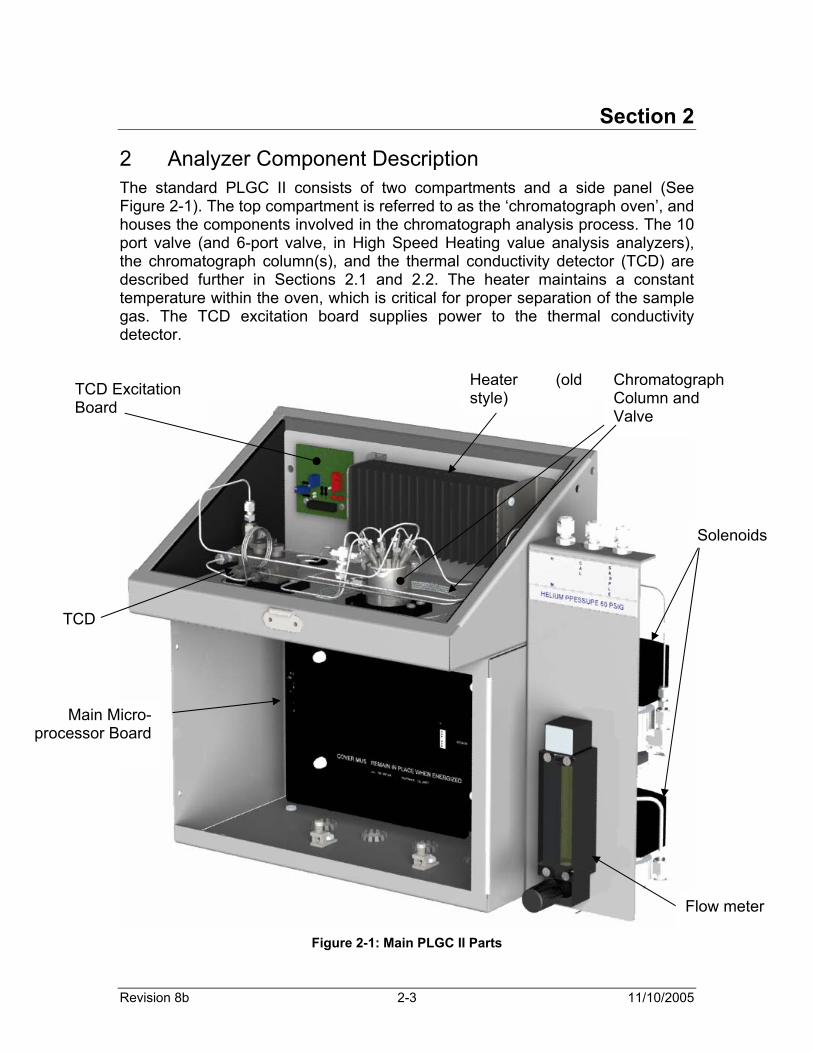
2 Analyzer Component Description The standard PLGC II consists of two compartments and a side panel (See Figure 2-1). The top compartment is referred to as the ‘chromatograph oven’, and houses the components involved in the chromatograph analysis process. The 10 port valve (and 6-port valve, in High Speed Heating value analysis analyzers), the chromatograph column(s), and the thermal conductivity detector (TCD) are described further in Sections 2.1 and 2.2. The heater maintains a constant temperature within the oven, which is critical for proper separation of the sample gas. The TCD excitation board supplies power to the thermal conductivity detector.
Figure 2-1: Main PLGC II Parts
Heater (old style)
Chromatograph Column and Valve
TCD
TCD Excitation Board
Main Micro-processor Board
Flow meter
Solenoids
Section 2 Part Number MA2182
2-4
The bottom compartment houses the PLGC II main microprocessor board. The microprocessor performs calculations, handles the Graphical User Interface (GUI), and controls communications for the chromatograph (See Section 2.3). The flow meter, gas inlet ports, and solenoids are located on the side panel. The flow meter controls the flow of sample gas into the PLGC II. In Figure 2-1, the top solenoid actuates the chromatograph valve, and the bottom solenoid switches between calibration gas and sample gas. If two or three chromatograph valves are to be used in the chromatograph application, additional solenoids can be wired to the analyzer. Solenoids can also be wired for switching up to 8 streams of gas. Solenoid wiring is explained in Section 4.1.1.
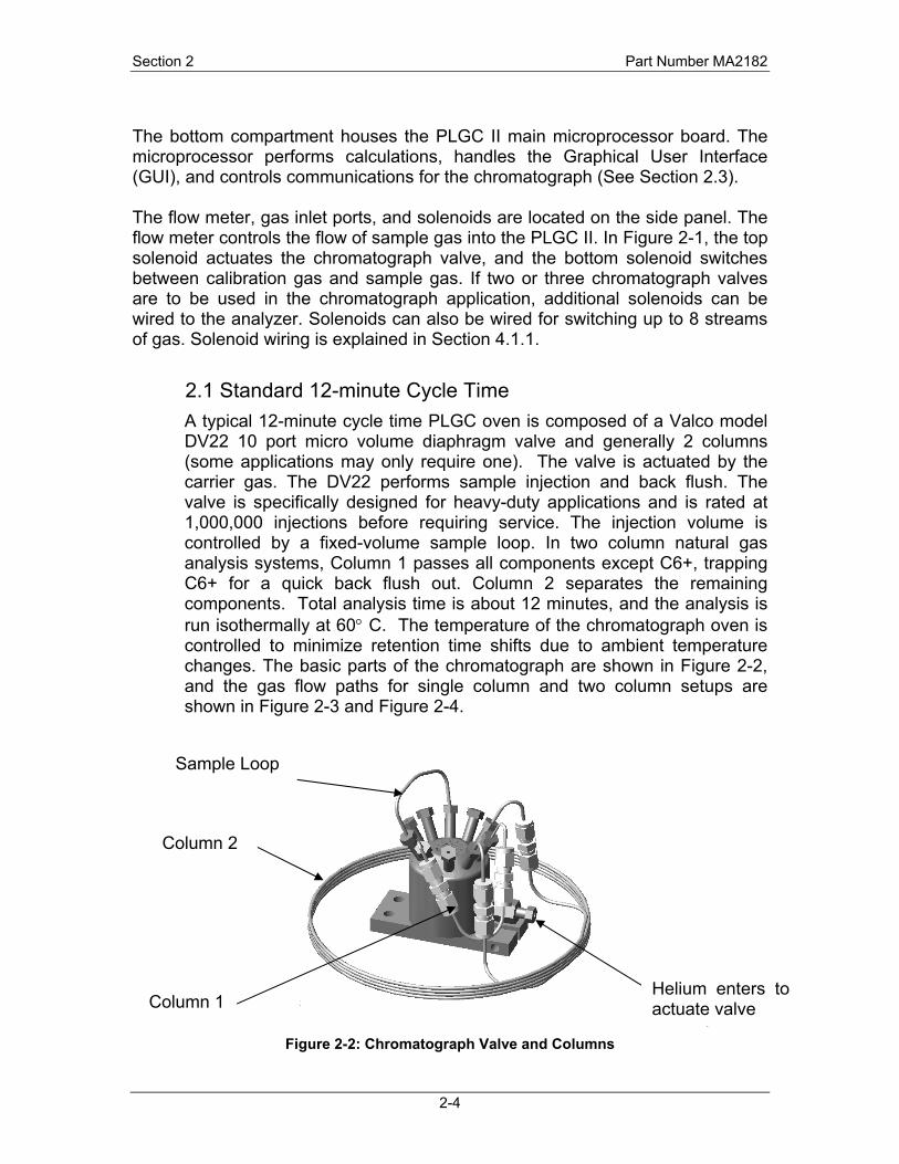
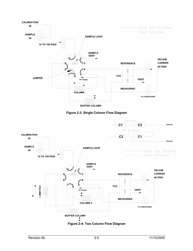
2.1 Standard 12-minute Cycle Time A typical 12-minute cycle time PLGC oven is composed of a Valco model DV22 10 port micro volume diaphragm valve and generally 2 columns (some applications may only require one). The valve is actuated by the carrier gas. The DV22 performs sample injection and back flush. The valve is specifically designed for heavy-duty applications and is rated at 1,000,000 injections before requiring service. The injection volume is controlled by a fixed-volume sample loop. In two column natural gas analysis systems, Column 1 passes all components except C6+, trapping C6+ for a quick back flush out. Column 2 separates the remaining components. Total analysis time is about 12 minutes, and the analysis is run isothermally at 60° C. The temperature of the chromatograph oven is controlled to minimize retention time shifts due to ambient temperature changes. The basic parts of the chromatograph are shown in Figure 2-2, and the gas flow paths for single column and two column setups are shown in Figure 2-3 and Figure 2-4.
Figure 2-2: Chromatograph Valve and Columns
Column 2
Column 1
Sample Loop
Helium enters to actuate valve
Revision 8b 2-5 11/10/2005
HELIUMCARRIER
INSAMPLE
SAMPLE LOOP
COLUMNMEASURING
REFERENCE
VENT
10 TO 100 PSIG
CALIBRATIONIN
JUMPER
12
3
4
56
7
8
9
SAMPLE VENT
10
Air Supply
TCD
TO ATMOSPHERE
BUFFER COLUMN
60 PSIG
HELIUMCARRIER
SAMPLE LOOP
CO
LUM
N 1
MEASURING
REFERENCE
VENT
12
3
4
56
7
8
9
SAMPLE VENT
10
Air Supply
C2
C1
C1
C2
Detector
Detector
COLUMN 2
BUFFER COLUMN
TCD
TO ATMOSPHERE
CALIBRATIONIN
INSAMPLE
10 TO 100 PSIG
60 PSIG
Figure 2-3: Single Column Flow Diagram
Figure 2-4: Two Column Flow Diagram

Section 2 Part Number MA2182
2-6
2.1.1 Rapid 4-Minute Analysis Cycle This application uses 2 DV22 micro volume diaphragm valves, one with ten ports and one with six ports. To facilitate the rapid analysis of the sample gas, a system comprised of four chromatograph columns is used. All components but C6+ pass through column 1, and C6+ is trapped by column 1 for a quick back flush out. Column 2 allows for the rapid passage of nitrogen, methane, and carbon dioxide into column 3, while separating the heavier hydrocarbon components – ethane, propane, i and n-butane, and i and n-pentane. Once carbon dioxide has entered column 3, the six-port valve is actuated, trapping nitrogen, methane, and carbon dioxide in column 3. The heavier components then pass through a jumper (marked in the diagram as R1), a short piece of tubing containing no packing material, on their way to the detector. Once n-pentane has eluted, the six-port valve is actuated a second time, and nitrogen, methane, and carbon dioxide then elute from column 3. Total analysis time is about 4 minutes, and as before the analysis is run isothermally at 60°C. The gas flow path for the HSHV analysis is shown in figure 2-5.
Figure 2-5: 4-minute analysis Flow Diagram
Revision 8b 2-7 11/10/2005
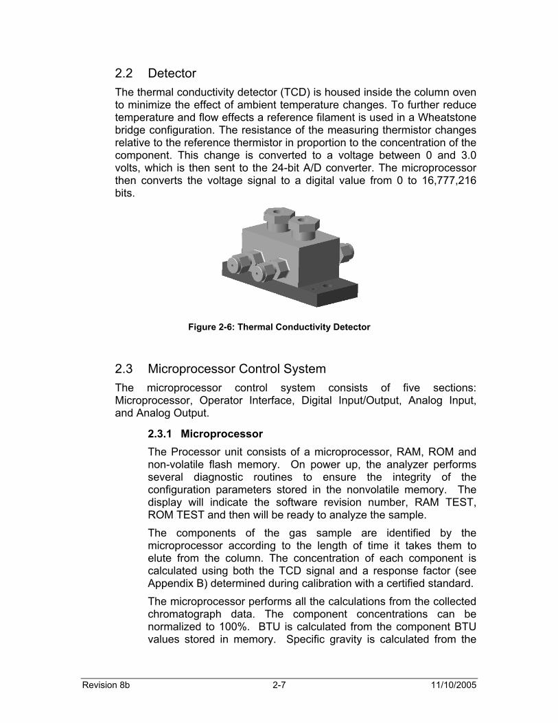
2.2 Detector The thermal conductivity detector (TCD) is housed inside the column oven to minimize the effect of ambient temperature changes. To further reduce temperature and flow effects a reference filament is used in a Wheatstone bridge configuration. The resistance of the measuring thermistor changes relative to the reference thermistor in proportion to the concentration of the component. This change is converted to a voltage between 0 and 3.0 volts, which is then sent to the 24-bit A/D converter. The microprocessor then converts the voltage signal to a digital value from 0 to 16,777,216 bits.
Figure 2-6: Thermal Conductivity Detector
2.3 Microprocessor Control System The microprocessor control system consists of five sections: Microprocessor, Operator Interface, Digital Input/Output, Analog Input, and Analog Output.
2.3.1 Microprocessor The Processor unit consists of a microprocessor, RAM, ROM and non-volatile flash memory. On power up, the analyzer performs several diagnostic routines to ensure the integrity of the configuration parameters stored in the nonvolatile memory. The display will indicate the software revision number, RAM TEST, ROM TEST and then will be ready to analyze the sample. The components of the gas sample are identified by the microprocessor according to the length of time it takes them to elute from the column. The concentration of each component is calculated using both the TCD signal and a response factor (see Appendix B) determined during calibration with a certified standard. The microprocessor performs all the calculations from the collected chromatograph data. The component concentrations can be normalized to 100%. BTU is calculated from the component BTU values stored in memory. Specific gravity is calculated from the

Section 2 Part Number MA2182
2-8
relative concentrations of each component and the specific gravity values stored in the microprocessor. The Wobbe Index can also be calculated from BTU and specific gravity. (See Appendix B)
2.3.2 Operator Interface The Operator Interface consists of an LCD display on the analyzer and a user interface program running on a standard PC (see software section for minimum requirements). Its function is to allow the user to configure the system as well as view the results of an analysis and any diagnostic functions. Section 5 discusses the operator interface in further detail.
2.3.3 Digital Input/Output The Digital Input/Output consists of eight status inputs, twelve high current solenoid drivers and four relays for alarm annunciation. See Section 4.1.1.
2.3.4 Analog Input The Analog Input consists of three 24 bit sigma delta a/d converters sampling at 60 times per second utilizing both analog and digital filtering techniques. See Section 4.1.2.
2.3.5 Analog Output The Analog Output consists of four 12-bit digital/analog converters and analog circuitry. See Section 4.1.3.

Revision 8b 3-9 11/10/2005
Section 3
3 Analyzer Installation and Considerations THE PLGC II DIVISION 2 EQUIPMENT IS SUITABLE FOR USE IN CLASS I, DIVISION 2, GROUPS B,C and D, or NON-HAZARDOUS LOCATIONS ONLY
Note: This symbol: ! means CAUTION. Wherever this symbol is seen, the user should make sure they are aware of all the dangers and precautions associated with the location of the symbol before proceeding.
3.1 Sampling Point Location The samples sent to the analyzer must be representative of the stream and should be taken from a point as close as possible to the analyzer to avoid lag times and sample degradation in the lines.
3.2 Sample Volume and Flow Rate Sample should be supplied to the analyzer at no more than 100 psig. A flow meter at the analyzer will control the flow into the analyzer's sample valve at 50 cc/min. A bypass sweep is recommended to reduce lag time in the sample lines.
3.3 Sample Conditioning The function of the sample system available as an option with the PLGC II is to regulate and filter the sample. The sample system is required if the sample is not available at a pressure less than 100 psig, contains particulates, or is subject to liquid dropout. Consideration must be taken of upset conditions as well as normal conditions when designing the sample system. Contamination is often a problem with PLGC II sample systems.
3.4 Battery WARNING: TO PREVENT IGNITION OF HAZARDOUS ATMOSPHERE, THE BATTERY MUST ONLY BE CHANGED IN AN AREA KNOWN TO BE NON-HAZARDOUS
Replace only with a battery of the following type: Tadrian TL-542/W
3.5 Installation The PLGC II analyzer was tested and configured at the factory. The program parameters are documented in the Configuration Report (enclosed with this manual).
Below is a step-by-step procedure for installing the instrument.
Section 3 Part Number MA2182
3-10
WARNING – Explosion Hazard – Substitution of components may impair suitability for Class I, Division 2 AVERTISSEMENT – Risque d’explosion – La substitution de composants peut render ce material inacceptable pour les emplacements de Classe I, Division 2 Step 1: Ensure that the selected installation site provides adequate room
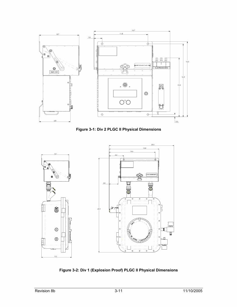
for opening the cabinet doors for maintenance and repair procedures. The site should be as close as possible to the process stream being measured. The dimensions of the PLGC II are shown Figure 3-1 and Figure 3-2.
Step 2: Unpack and Check for Damage Step 3: Attach UHP helium at the pressure specified in the factory setup
(usually 60 psig). A dual stage regulator is recommended. See to see where to attach the helium.
Step 4: Ensure that the vent (shown in) is to atmospheric pressure, on a
downward slope. Step 5: Wire the appropriate power to the analyzer and allow the oven
temperature to reach the set temperature (usually 40° C). If possible allow the analyzer to stabilize over night. Note that mains supply voltage fluctuations are not to exceed 10 percent of the nominal supply voltage.
Note:
- A switch or circuit breaker shall be included in the building installation
- The switch/circuit breaker shall be in close proximity to the equipment and within easy reach of the operator
- The switch/circuit shall be marked as the disconnecting device for the equipment.
Revision 8b 3-11 11/10/2005
1.8
11.8
16.7
0.5
13.0
16.0
16.5
6.8
8.7
Figure 3-1: Div 2 PLGC II Physical Dimensions
2.8
4.6
14.6
15.8
20.5
29.9
8.7
9.5
Figure 3-2: Div 1 (Explosion Proof) PLGC II Physical Dimensions
Section 3 Part Number MA2182
3-12
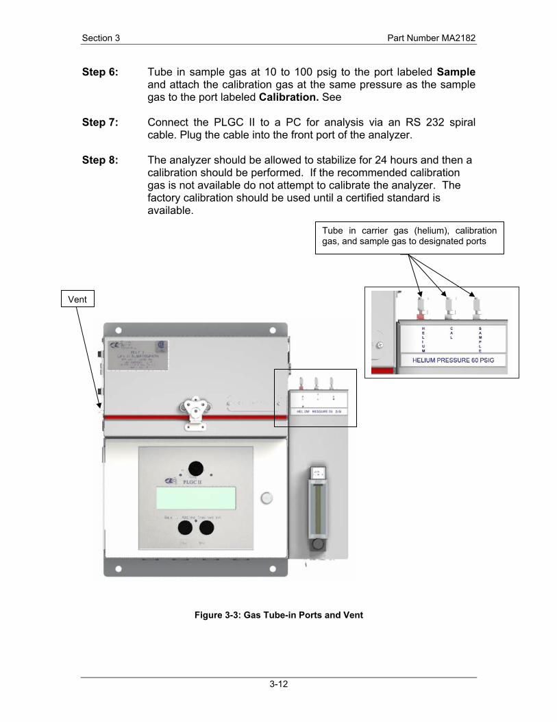
Step 6: Tube in sample gas at 10 to 100 psig to the port labeled Sample and attach the calibration gas at the same pressure as the sample gas to the port labeled Calibration. See
Step 7: Connect the PLGC II to a PC for analysis via an RS 232 spiral
cable. Plug the cable into the front port of the analyzer. Step 8: The analyzer should be allowed to stabilize for 24 hours and then a
calibration should be performed. If the recommended calibration gas is not available do not attempt to calibrate the analyzer. The factory calibration should be used until a certified standard is available.
Figure 3-3: Gas Tube-in Ports and Vent
Tube in carrier gas (helium), calibration gas, and sample gas to designated ports
Vent

Revision 8b 4-13 11/10/2005
Section 4
4 Electrical Connections and Considerations
4.1 Functions of Electrical Ports Figure 4-1 shows a diagram of the main PLGC II board. The functions of the individual electrical ports on this board are described in this section.
Figure 4-1: Main PLGC II Board

Section 4 Part Number MA2182
4-14
4.1.1 Digital Input/Output and Power
Figure 4-2: Digital Input and Output
Input Power: 24V DC 3A power to main board
Digital Input/Output: Relays: These can be configured to trigger alarms, status
information, or `fail information at various set limits. They are primarily used for indicating alarms, fails, or analyzer status. Digital Inputs: Status Inputs that can be used for connection of external pressure and temperature switches. Input ‘1’ is generally wired for a Calibration Initiation switch. Stream Select Valve Drivers 1-8: Solenoid actuation for stream switching up to 8 streams.
Revision 8b 4-15 11/10/2005
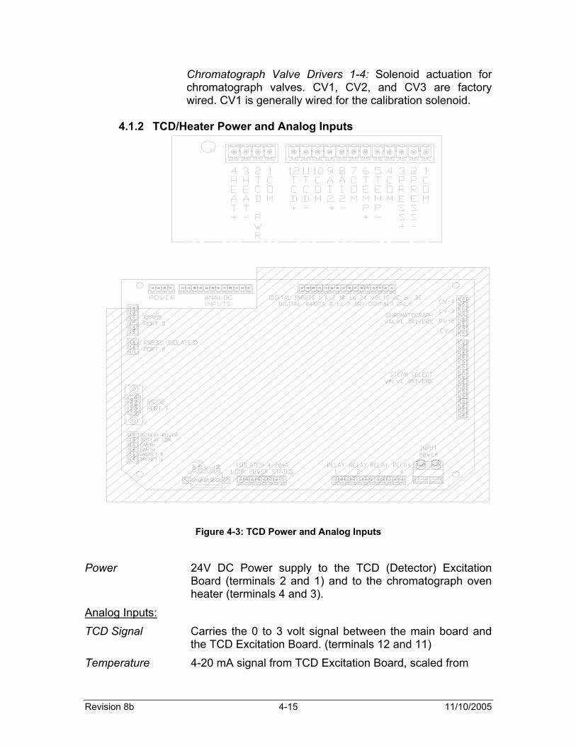
Chromatograph Valve Drivers 1-4: Solenoid actuation for chromatograph valves. CV1, CV2, and CV3 are factory wired. CV1 is generally wired for the calibration solenoid.
4.1.2 TCD/Heater Power and Analog Inputs
Figure 4-3: TCD Power and Analog Inputs
Power 24V DC Power supply to the TCD (Detector) Excitation
Board (terminals 2 and 1) and to the chromatograph oven heater (terminals 4 and 3).
Analog Inputs: TCD Signal Carries the 0 to 3 volt signal between the main board and
the TCD Excitation Board. (terminals 12 and 11) Temperature 4-20 mA signal from TCD Excitation Board, scaled from

Section 4 Part Number MA2182
4-16
0°C – 100°C (terminals 6 and 5) Pressure Auxiliary 4-20 mA input (Not factory wired – terminals 3 and
2) 4.1.3 Modbus Ports
Figure 4-4: Modbus Connection Ports
RS 232 Port 1 A non-isolated RS 232 Modbus communication port. Pin Configuration for Port 1:
Pin 2 TX Pin 3 RX Pin 5 GND RS 232 (Isolated) Port 2 An isolated RS 232 Modbus communication port RS 485 Port 3 An isolated RS 485 port for Modbus communication

Revision 8b 4-17 11/10/2005
See Figure 4-6 for further information on Modbus wiring.
4.1.4 Analog Output and ‘ARCNET’
Figure 4-5: Analog Output and ‘ARCNET’
ARCNET A high speed networking architecture that allows multiple
analyzers to share data, and allows remote configuration of multiple analyzers from a single unit.
Analog Output 4-20 mA outputs that are programmable and can be used for a number of output applications. A powered loop is required for these outputs. The polarity (+/-) for these ports is shown in Figure 4-5
Section 4 Part Number MA2182
4-18
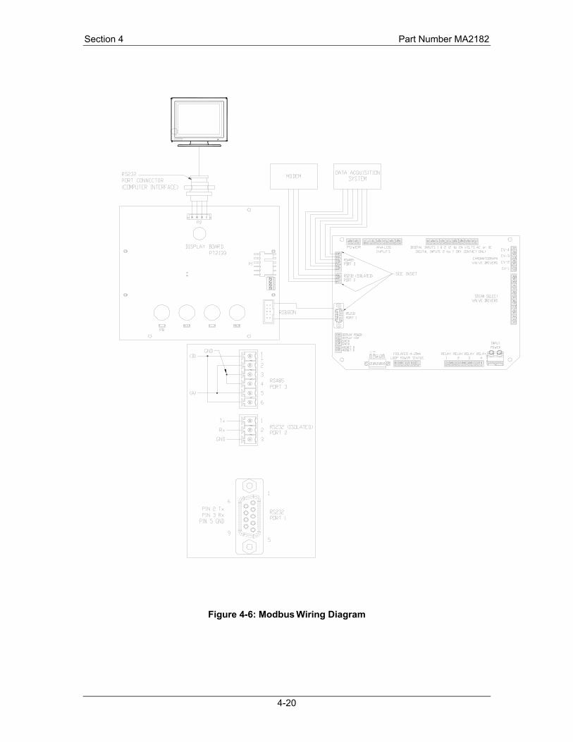
4.2 Modbus Communication The PLGC II has Modbus communication on two RS-232 ports and one RS-485 port on board. They can be used to retrieve historical archives and allow configuration and monitoring of the PLGC II. One of the RS-232 ports is isolated. On power-up, the unit will complete an initial startup. The wiring for Modbus communications is shown in Figure 4-6.
The standard PLGC II has three serial ports. These ports can be used to configure the analyzer or as Modbus communications ports as follows:
4.2.1 Enron Modbus Protocol: RTU Data Transfer Format ASCII Data Transfer Format Selectable - 300 to 115200 bps Selectable – 300 to 115200 bps No Parity Even Parity 8 Data bits 7 Data bits 1 Stop bit 1 Stop bit The PLGC II analyzer can be configured for different baud rates in different modes. The analyzer will be set up for Enron Modus communications at 9600 RTU mode as sent from the factory.
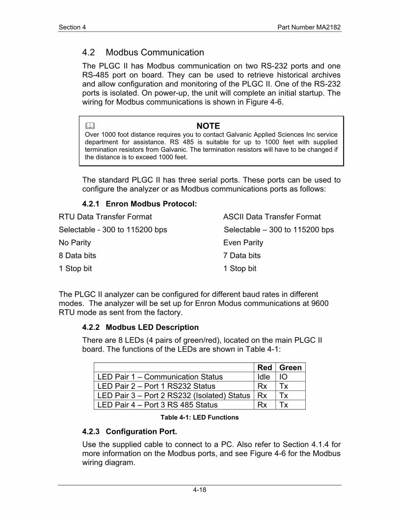
4.2.2 Modbus LED Description There are 8 LEDs (4 pairs of green/red), located on the main PLGC II board. The functions of the LEDs are shown in Table 4-1:
Red Green LED Pair 1 – Communication Status Idle IO LED Pair 2 – Port 1 RS232 Status Rx Tx LED Pair 3 – Port 2 RS232 (Isolated) Status Rx Tx LED Pair 4 – Port 3 RS 485 Status Rx Tx
Table 4-1: LED Functions
4.2.3 Configuration Port. Use the supplied cable to connect to a PC. Also refer to Section 4.1.4 for more information on the Modbus ports, and see Figure 4-6 for the Modbus wiring diagram.
NOTE Over 1000 foot distance requires you to contact Galvanic Applied Sciences Inc service department for assistance. RS 485 is suitable for up to 1000 feet with supplied termination resistors from Galvanic. The termination resistors will have to be changed if the distance is to exceed 1000 feet.

Revision 8b 4-19 11/10/2005
Section 4 Part Number MA2182
4-20
Figure 4-6: Modbus Wiring Diagram

Revision 8b 4-21 11/10/2005
4.3 PLGC II Wiring Schedule The wiring schedule shown in Table 4-2 should be used in conjunction with the wiring diagram. See Section 4.4. Electrical Connection
Description Terminal 1 Terminal 2 Wire
Colour Signal Name
TCD Excitation Board TCD Board - P2 RTD Red A TCD Board - P2 RTD Black B TCD Board - P2 RTD Black B TCD Board - P2 TCD Blue TCD Blue TCD Board - P2 TCD Red TCD Red TCD Board - P2 TCD Red TCD Red TCD Board - P2 TCD Green TCD Green
Main – 2 TCD PWR (P6) TCD Board - P1-2 Red +24 vdc Main – 1 COM (P6) TCD Board - P1-1 Black 0 vdc
Main – 5 TEMP – (P5) TCD Board - P1-3 Green RTD com
Main – 6 TEMP + (P5) TCD Board - P1-4 Brown RTD 4-20
Main – 12 TCD + (P5) TCD Board - P1-5 White TCD + Main – 11 TCD – (P5) TCD Board - P1-6 Blue TCD -
TCD Excitation Board to Main board. -AWG 24, 6 conductor plus shield stranded wire. -For explosion proof version, these connections are made through an I.S. Barrier. See Figure 4-8 Main – 1 COM Thick Green Shield
Main – 4 HEAT + (P6)
Heater (+/ -) Blue Heater A Heater to main board - AWG18 blue (24VDC) - Either wire can be connected to either port
Main – 3 HEAT – (P6) Heater (+/ -) Blue Heater B
Main – 4 HEAT + (P6) Heater Relay + Red Heater + Heater to Main Board Red/Black (110/220VAC) Main – 3HEAT – (P6) Heater Relay - Black Heater -
Calibration Sol.
Main – CV 1(+ or -) Calibration Solenoid (+/-)
Red Cal A
Main – CV 1(+ or -) Calibration Solenoid (+/-)
Red Cal B
Valve Sol. Main – CV 2(+ or -) Valve 1 Solenoid (+/-) Red Valve 1 A Main – CV 2 (+ or -) Valve 1 Solenoid (+/-) Red Valve 1 B Main – CV 3 (+ or -) Valve 2 Solenoid (+/-) Red Valve 2 A
Solenoids to main board -24 V nominal -Either wire can be connected to either port
Main – CV 3 (+ or -) Valve 2 Solenoid (+/-) Red Valve 2 B Main – 1 DISPLAY PWR (P10) Display - P10-4 (24V) Red +24 VDC Display to main board
-AWG 22 red and black’ Main – 2 DISPLAY COM (P10) Display - P10-1 (GND) Black 0 VDC
RS232 ribbon cable Main - P13 Display - P4 Ribbon Cable
RS232
Main – COM 1 (P11) Green
Main – COM 2 (P11) Black
Main – INT 3 (P11) Red
Main – SCL 4 (P11) White
Display data beldon cable -Orange connector connects to Display Board P1 - Other end of beldon cable is stripped and contains 5 coloured wires Main – SDA 5 (P11)
Display - P1
Brown
Display
Table 4-2: PLGC II Wiring Schedule
Section 4 Part Number MA2182
4-22
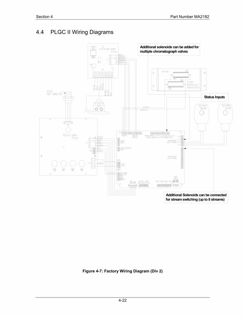
4.4 PLGC II Wiring Diagrams
Additional Solenoids can be connected for stream switching (up to 8 streams)
Status Inputs
Additional solenoids can be added for multiple chromatograph valves
Figure 4-7: Factory Wiring Diagram (Div 2)
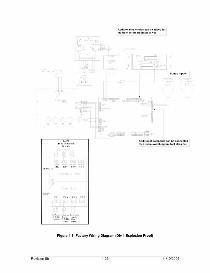
Revision 8b 4-23 11/10/2005
Additional Solenoids can be connected for stream switching (up to 8 streams)
Status Inputs
Additional solenoids can be added for multiple chromatograph valves
Figure 4-8: Factory Wiring Diagram (Div 1 Explosion Proof)


Revision 8b 5-25 11/10/2005
Section 5
5 Software Operation This section describes basic operations of the PLGC software. It is based on the assumption that the analyzer has been correctly configured at the factory. The PLGC II software has been designed to receive, interpret, and plot data from the PLGC II gas chromatograph. Peaks in the resulting chromatogram identify the compound by retention time and the concentration by the area of the peak. Various parameters, including BTU, specific gravity, and compressibility factor, can be displayed with the software. The Graphical User Interface (GUI) for the software is a Windows-based system. This manual provides instructions on the installation, setup and use of the PLGC II software program. It includes requirements and procedures for installation along with instructions for communication between the chromatograph and computer. It also outlines procedures for calibration, configuration and data acquisition. Once the software has been installed, it is possible to view the software Revision History by clicking the ‘Help’ menu at the top of the screen and choosing ‘View Revision History’.
5.1 Software Installation and Connection 5.1.1 System Requirements The following are the computer requirements to install and operate the PLGC II software.
Operating System Microsoft Windows 98, Me, 2000, or XP Memory Minimum of 64MB RAM. Disk Drives A CD ROM drive is required to read the installation disk, and a minimum of 20 megabytes of space is required for installation on the PC hard drive. More space will be required to save data, such as chromatograms and archive data. Serial Port The PLGC connects to the PC with an RS-282 serial cable, requiring a 9-pin male serial connector, as seen in Figure 5-1.

Section 5 Part Number MA2182
5-26
Figure 5-1: 9-Pin Male Serial Port
It is important to note that the 9-Pin male serial connector can be on a USB-Serial adapter, provided that the USB to serial adapter is correctly configured. Also, the COM port used for connecting to the PLGC cannot be used for any other purposes; otherwise connecting to the PLGC II will not be possible.
5.1.2 Software Installation Insert the PLGC II software configuration CD into the CD drive. The disc should auto-run, and will prompt the user as to how to proceed. In the event that the disc does not auto-run, follow these instructions:
1. In the lower-left hand corner of the screen select the ‘Start’ button then select ‘Run’ from the Start menu.
2. Type in the drive designation for the optical drive (e.g. D:\) followed by setup.exe.
3. Press enter and follow the instructions given.
5.1.3 Connecting PLGC II to PC Connect the provided RS 232 cable to the serial port located on the front panel of the PLGC II, shown in Figure 5-2.
Figure 5-2: PLGC II Front Panel Connector
Connect the other end of the cable to a male 9-pin serial port on the back of the computer, or attached to a USB-Serial adapter that has been correctly configured.
5.2 Interface and Icons The GUI is a Windows-based, point and click interface. There are two main rows of buttons at the top of the main screen. These rows can be dragged and positioned around the screen border as the user desires. The following is a brief description of each of these buttons.

Revision 8b 5-27 11/10/2005
Open – allows the user to open a pre-saved configuration. This button can only be used if the PC is not connected to the PLGC II.
Save Current Configuration - allows the user to save a currently open configuration. This can only be used if the open configuration has already been named.
Save As – allows the user to save a currently open configuration to a new file.
Save All – allows the user to save configuration files for all open windows.
Print – allows the user to print to print the output from the currently open window, including action lists, component tables, chromatograms, and archive data.
Tile Windows – allows the user to see all open windows on one screen.
Cascade Windows – allows the user to reduce the size of all open windows and lines them up one behind the next.
Arrange – allows the user to arrange all minimized windows.
Close All - allows the user to close all open windows.
Collapse – allows the user to collapse the directory tree on the left side of the screen.
Expand All – allows the user to expand all branches of the directory tree on the left side of the screen
Logon – Establishes a communication link between the computer and the PLGC II.
Logoff – Disconnects the communication link between the computer and the PLGC II.

Section 5 Part Number MA2182
5-28
Communications Setup – Allows the user to set up communications options.
Read Current – Reads data from device for active window.
Write Current – Writes configuration to device from active window. This button MUST be pushed any time configuration changes are made in any PLGC application window.
Read All – Reads data from device for all open windows.
Write All – Writes configuration to device from all open windows.
Polling – Poll data continuously for all open windows.
Synchronize Time – updates PLGC II time and date with the time and date set on the connected PC. Ensure that the PC’s time and date is set correctly before synchronizing time.
Process Monitor – allows the user to view the revision number for all applications installed on the PLGC. This is useful for troubleshooting. See Section 5.6.1, Advanced Operations – Factory Mode for more information.
In addition, there are two more icons that are available in ‘Factory’ Mode. Factory mode, as the name would suggest, is a mode that allows the user to update or remove applications installed on the PLGC II. For more information, see Section 5.6.1, Advanced Operations – Factory Mode. The icons are shown below.
Update Firmware – allows the user to update any or all applications installed on the PLGC if new updates are provided from Galvanic Applied Sciences Inc.
Wipe All Processes – allows the user to wipe all processes (applications) from the PLGC II board. This should ONLY be used at the factory or by trained service Personnel.
5.2.1 Logging on to the PLGC II To establish a communication link between the computer and the PLGC II, open the program by double-clicking the DIMAC icon. Ensure that the
Revision 8b 5-29 11/10/2005
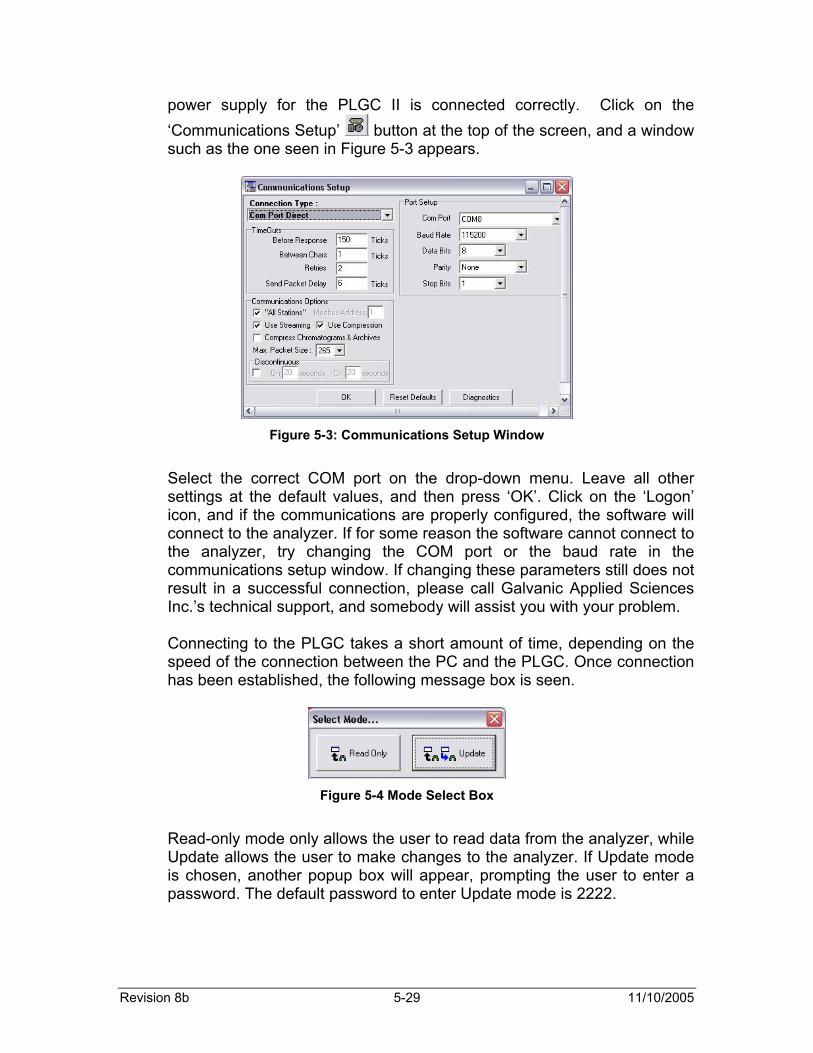
power supply for the PLGC II is connected correctly. Click on the ‘Communications Setup’ button at the top of the screen, and a window such as the one seen in Figure 5-3 appears.
Figure 5-3: Communications Setup Window
Select the correct COM port on the drop-down menu. Leave all other settings at the default values, and then press ‘OK’. Click on the ‘Logon’ icon, and if the communications are properly configured, the software will connect to the analyzer. If for some reason the software cannot connect to the analyzer, try changing the COM port or the baud rate in the communications setup window. If changing these parameters still does not result in a successful connection, please call Galvanic Applied Sciences Inc.’s technical support, and somebody will assist you with your problem.
Connecting to the PLGC takes a short amount of time, depending on the speed of the connection between the PC and the PLGC. Once connection has been established, the following message box is seen.
Figure 5-4 Mode Select Box
Read-only mode only allows the user to read data from the analyzer, while Update allows the user to make changes to the analyzer. If Update mode is chosen, another popup box will appear, prompting the user to enter a password. The default password to enter Update mode is 2222.

Section 5 Part Number MA2182
5-30
5.3 Database and Devices In the left hand window of the main program area, there are two tabs to choose from: ‘Devices’ and ‘Database’. Clicking on either of these tabs will open up a different ‘tree’.
5.3.1 Database The database is the part of the software that defines all of the parameters required to operate the analyzer. When the tab is first opened, the tree view shown in Figure 5-5 is seen.
Figure 5-5: Default Database Tree View
There are 3 major categories in the database – simple data points, archives, and global data points. The first two categories, Simple Data Points and Archives, contain information that can be output to MODBUS lists. Simple data points contain data related to the various processes installed on the PLGC, while the Archives section contains archive records. To get information about the database, right-click anywhere on the white field and choose the ‘What’s This?’ option from the pop-up menu that appears. This will provide a brief description of the database. Further, right-clicking on any label in the database will also bring up a pop-up menu with ‘What’s This?’ being the top option on the menu. This will provide slightly more detail about the given group of data points in the database. The most important section of the Database is the section that contains the Global Data Points (GDPs). When the ‘+’ sign next to Global Data Points is clicked, the two sub-categories shown in Figure 5-6 are seen.
Figure 5-6: Global Data Points
I/O Controls are all of the data points relevant to the mechanical and electrical operation of the analyzer. Under I/O controls can be found discrete inputs, relays, chromatograph valves, solenoids, and inputs from the detector and the RTD that measures the temperature in the

Revision 8b 5-31 11/10/2005
chromatograph oven. An expanded view of the I/O Controls sub-category is seen in Figure 5-7.
Figure 5-7: Database I/O Controls
Each individual control is referred to as a ‘control point’. Any control point, be it a relay, solenoid, valve, or anything else, can be dragged from the database window into an open window on the right hand side of the screen (see Section 5.5.3 – Streams and Section 5.5.4 – Sample Handling for more information). Additional GDPs are the data points in which all collected data is stored. In this section, data points are created that store data from BTU calculations, specific gravity calculations, component values, and any other numerical values calculated or recorded by the PLGC. Each data point contains information about the current value of the data point, as well as hourly, daily, and monthly maxima, minima, averages, and analysis counts. Additional GDPs must be set up in stream setups (see section 5.5.3.2)

Section 5 Part Number MA2182
5-32
and can be stored in the PLGC’s onboard memory in archives (see section 5.4.2 – Archive Reader, and 5.5.7, Archive Setup).
There are several other options on the pop-up menu that appears when a GDP label is right-clicked on.
• Expand Selected Node – if the label has a ‘+’ sign to the left of it, choosing this option will cause this portion of the database to expand, showing sub-categories.
• Collapse Tree – collapses the database down to the root, showing only the ‘DIMAC Network Database’ Label
• Expand Tree – expands all nodes within the database tree • Save Database – saves the entire database to a database
(*.DCDB) file • Load Database – loads a previously saved database from a file. • Write DB Changes to Unit – sends the updated database to the
analyzer. • Create new GDP – creates a new global data point with a name of
the user’s choosing. The following window appears to create a new GDP.A name for the new GDP is placed in the ‘Name’ field, while typically the ‘Type’ field is left at the default ‘Scalar’. When ‘Scalar’ is chosen, no units are necessary. New GDPs are created in the ‘Additional GDPs’ section of the database.
In addition, if the label right-clicked on is a single GDP, rather than a Node name, the following additional options are available.
• Delete GDP – deletes the selected GDP. However, if the GDP is referenced anywhere in any process in the PLGC, the software will not allow that GDP to be deleted. The message box shown in Figure 5-8 shows the message that appears when attempting to delete a referenced GDP
. Figure 5-8: Cannot Delete GDP Message Box
Revision 8b 5-33 11/10/2005
The message box also shows exactly where the given GDP is referenced – in this particular example, the GDP is referenced in two locations, one in a Stream, the other in an Archive.
• Modify GDP – allows the user to change the name, type, and units of a given GDP.
• Show Where GDP Is Used – brings up a box similar to that shown in Figure 5-8 that shows all processes where the given GDP is referenced.
• Configure Alarms – this feature is not currently working, but will be operational in later versions of the software.
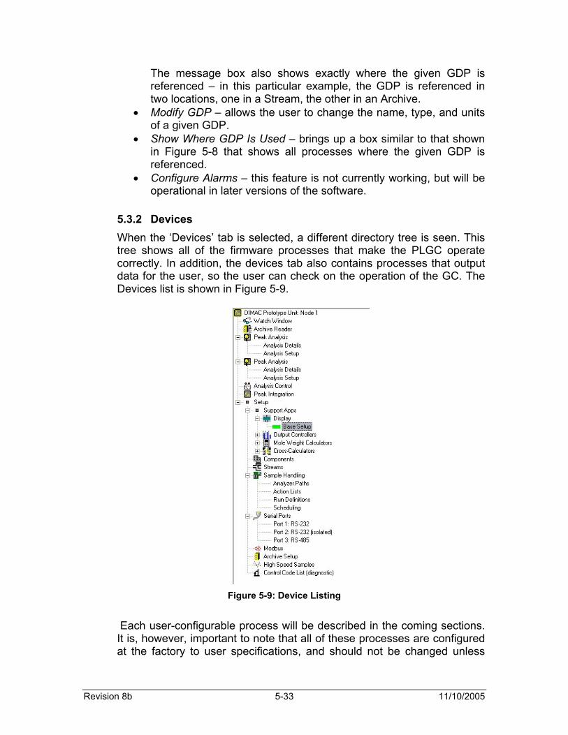
5.3.2 Devices When the ‘Devices’ tab is selected, a different directory tree is seen. This tree shows all of the firmware processes that make the PLGC operate correctly. In addition, the devices tab also contains processes that output data for the user, so the user can check on the operation of the GC. The Devices list is shown in Figure 5-9.
Figure 5-9: Device Listing
Each user-configurable process will be described in the coming sections. It is, however, important to note that all of these processes are configured at the factory to user specifications, and should not be changed unless
Section 5 Part Number MA2182
5-34
absolutely necessary. The processes will be described in the order that they are listed in the Devices tree. Right-clicking on any label in the Devices tree will bring up a pop-up menu whose top option is ‘What’s This?’. Clicking ‘What’s This?’ will provide a brief pop-up description of the purpose of the given process.
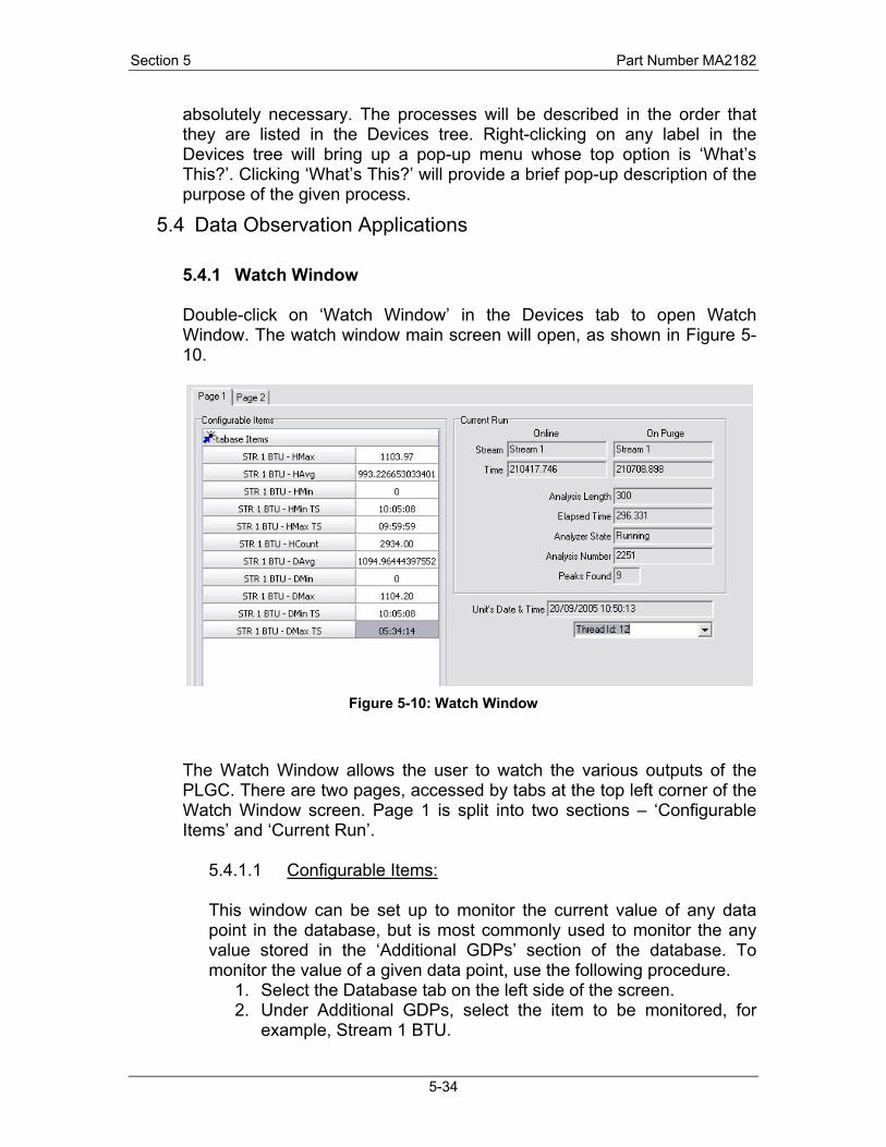
5.4 Data Observation Applications 5.4.1 Watch Window Double-click on ‘Watch Window’ in the Devices tab to open Watch Window. The watch window main screen will open, as shown in Figure 5-10.
Figure 5-10: Watch Window
The Watch Window allows the user to watch the various outputs of the PLGC. There are two pages, accessed by tabs at the top left corner of the Watch Window screen. Page 1 is split into two sections – ‘Configurable Items’ and ‘Current Run’.
5.4.1.1 Configurable Items:
This window can be set up to monitor the current value of any data point in the database, but is most commonly used to monitor the any value stored in the ‘Additional GDPs’ section of the database. To monitor the value of a given data point, use the following procedure.
1. Select the Database tab on the left side of the screen. 2. Under Additional GDPs, select the item to be monitored, for
example, Stream 1 BTU.
Revision 8b 5-35 11/10/2005
3. Left click and hold on the given GDP, and drag it over into the ‘Configurable Items’ window. This will put the current value of this GDP into the window.
4. To monitor hourly, daily, or monthly minima, maxima, or averages, or the previous value of the GDP, first press the ‘+’ to the left of the GDP. Under each GDP are listed Current Value TS (timestamp), Previous Value (the value recorded immediately before the current value), Previous Value TS, and hourly, daily, and monthly trends. In the trends subsections are found minima, maxima, averages, and timestamps for the minima and maxima. Any of these can be dragged into the ‘Configurable Items’ window by following the instructions in step 3.
5. Once all the desired GDP values have been dragged into the ‘Configurable Items’ window, click on the ‘Write Current’ button at the top of the screen. Then, to see the value for each chosen GDP, click on the ‘Read Current’ button, and numerical values for each GDP will be seen.
5.4.1.2 Current Run
This box shows information about the current status of the PLGC. It shows which stream is currently being analyzed, which stream is being purged, the total time (in seconds) that the analyzer has been operating, analysis length (also in seconds), elapsed time, analyzer state (running or halted), analysis number (the total number of analyses run since the analyzer was powered up), and the number of peaks found in the current analysis. Also, at the bottom of the screen is the current analyzer time. If this is not the same as the time on the PC, time synchronization should be performed.
5.4.1.3 Watch Window Page 2
Page 2 of the watch window has no user-configurability. It shows the current outputs from the Column Oven PID controller (see Section 5.5.1.2.1), other analog outputs (see section 5.5.1.2.2), and all calculated values from the Mol Weight Controllers (see section 5.5.1.3) and Cross Calculators (see Section 5.5.1.4). It’s a convenient page because it allows the user to see all the important outputs from the PLGC on one page. Page 2 of the Watch Window is shown in Figure 5-11.

Section 5 Part Number MA2182
5-36
Figure 5-11: Watch Window Page 2
5.4.2 Archive Reader The PLGC II contains a large quantity of on-board memory for storage of analysis data and analyzer outputs. The purpose of the Archive Reader is to retrieve this data and output it. The PLGC II is configured at the factory with a standard archive configuration – to add or change the archive configuration, please see section 5.5.7, Archive Setup. To open the Archive Reader window, double-click on Archive Reader in the Devices tab. The main window of the Archive Reader is seen in Figure 5-12.
Figure 5-12: Archive Reader Window
To read an archive, choose an archive from the pull-down menu at the top of the window, select the number of records to pull (the valid range is shown on the button to the right of this box – press the button to
Revision 8b 5-37 11/10/2005
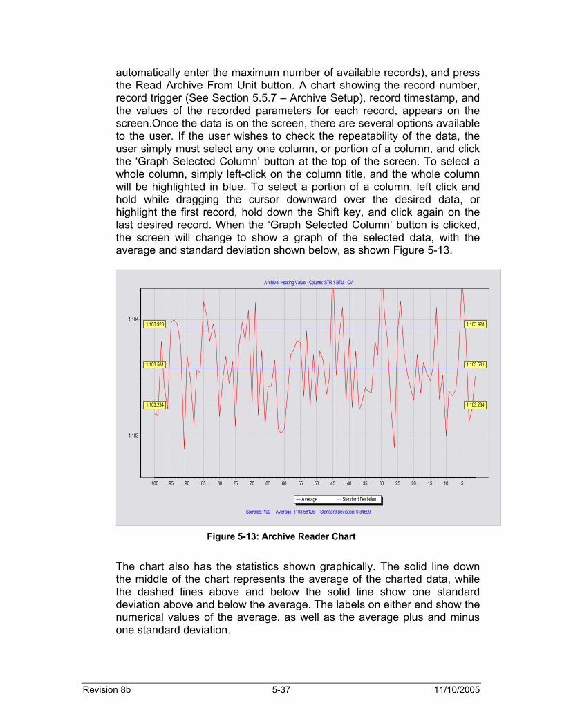
automatically enter the maximum number of available records), and press the Read Archive From Unit button. A chart showing the record number, record trigger (See Section 5.5.7 – Archive Setup), record timestamp, and the values of the recorded parameters for each record, appears on the screen.Once the data is on the screen, there are several options available to the user. If the user wishes to check the repeatability of the data, the user simply must select any one column, or portion of a column, and click the ‘Graph Selected Column’ button at the top of the screen. To select a whole column, simply left-click on the column title, and the whole column will be highlighted in blue. To select a portion of a column, left click and hold while dragging the cursor downward over the desired data, or highlight the first record, hold down the Shift key, and click again on the last desired record. When the ‘Graph Selected Column’ button is clicked, the screen will change to show a graph of the selected data, with the average and standard deviation shown below, as shown Figure 5-13.
Archive: Heating Value - Column: STR 1 BTU - CV
Samples: 100 Average: 1103.58126 Standard Deviation: 0.34699
Average Standard Deviation
100 95 90 85 80 75 70 65 60 55 50 45 40 35 30 25 20 15 10 5
1,104
1,103
1,103.5811,103.581
1,103.2341,103.234
1,103.9281,103.928
Figure 5-13: Archive Reader Chart
The chart also has the statistics shown graphically. The solid line down the middle of the chart represents the average of the charted data, while the dashed lines above and below the solid line show one standard deviation above and below the average. The labels on either end show the numerical values of the average, as well as the average plus and minus one standard deviation.

Section 5 Part Number MA2182
5-38
Right-clicking on the chart gives several options. • Set Scale – allows the user to either set his or her desired y-axis
scaling (scale manually) or to have the program automatically scale the y-axis to the selected data (scale to data).
• Print – allows the user to print the chart. Ensure that there is a printer set up on the PC prior to selecting this option.
• Copy to Clipboard – allows the user to copy the chart as an image to the clipboard, for pasting into another application such as Microsoft Word.
• Preferences – allows the user to change various display preferences for the chart:
o Set Trace Colour – allows the user to change the colour of the actual chart (data) and/or the statistics lines (statistics)
o Set Background Colour – allows the user to change the background colour
o Reset Default Colours – allows the user to return to the default colours for the chart – grey background, red data, and blue lines for statistics.
o Invert Scrolling – changes the effect the arrow keys have on scrolling zoomed data. Down scrolls up, left scrolls right, etc.
o Print Orientation/Print Sizing – sets options for printing the chart.
o Show Statistics – toggles whether or not the statistics labels are present.
To return to the raw data, click on the ‘Table’ tab in the upper right-hand corner of the Archive window. There are also several right-click options available in the ‘Table’ tab.
• Print Preview – previews the printout of the archive data. • Print – allows the user to print the raw data table. • Load from File – allows the user to load a saved archive data file in
proprietary Galvanic format (*.dcar). • Save to File – allows the user to save the archive data to a *.dcar
file. • Save as XLS – allows the user to save the archive data to a
Microsoft Excel (*.xls) file. • Copy Selection To Clipboard – allows the user to copy a selected
column of data to the clipboard. (only available if there is a highlighted portion of data)
• Copy Image to Clipboard – copies the entire archive window as an image to the clipboard so that it can be pasted into another application.
• Hide Selected Column – hides any selected columns (only available if one or more complete columns are highlighted).
• Unhide All Columns – shows all columns, including any that have been previously hidden.
Revision 8b 5-39 11/10/2005
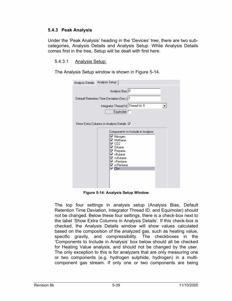
5.4.3 Peak Analysis Under the ‘Peak Analysis’ heading in the ‘Devices’ tree, there are two sub-categories, Analysis Details and Analysis Setup. While Analysis Details comes first in the tree, Setup will be dealt with first here.
5.4.3.1 Analysis Setup: The Analysis Setup window is shown in Figure 5-14.
Figure 5-14: Analysis Setup Window
The top four settings in analysis setup (Analysis Bias, Default Retention Time Deviation, Integrator Thread ID, and Equimolar) should not be changed. Below these four settings, there is a check-box next to the label ‘Show Extra Columns in Analysis Details’. If this check-box is checked, the Analysis Details window will show values calculated based on the composition of the analyzed gas, such as heating value, specific gravity, and compressibility. The checkboxes in the ‘Components to Include in Analysis’ box below should all be checked for Heating Value analysis, and should not be changed by the user. The only exception to this is for analyzers that are only measuring one or two components (e.g. hydrogen sulphide, hydrogen) in a multi-component gas stream. If only one or two components are being
Section 5 Part Number MA2182
5-40
measured, it is not essential to have all components included in the analysis.
5.4.3.2 Analysis Details
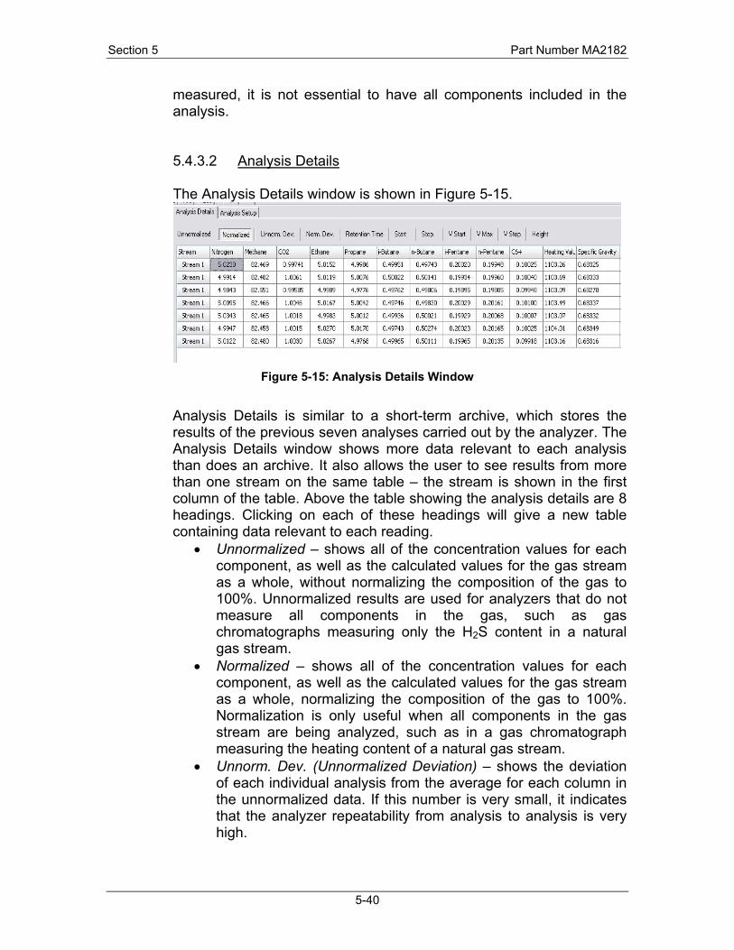
The Analysis Details window is shown in Figure 5-15.
Figure 5-15: Analysis Details Window
Analysis Details is similar to a short-term archive, which stores the results of the previous seven analyses carried out by the analyzer. The Analysis Details window shows more data relevant to each analysis than does an archive. It also allows the user to see results from more than one stream on the same table – the stream is shown in the first column of the table. Above the table showing the analysis details are 8 headings. Clicking on each of these headings will give a new table containing data relevant to each reading.
• Unnormalized – shows all of the concentration values for each component, as well as the calculated values for the gas stream as a whole, without normalizing the composition of the gas to 100%. Unnormalized results are used for analyzers that do not measure all components in the gas, such as gas chromatographs measuring only the H2S content in a natural gas stream.
• Normalized – shows all of the concentration values for each component, as well as the calculated values for the gas stream as a whole, normalizing the composition of the gas to 100%. Normalization is only useful when all components in the gas stream are being analyzed, such as in a gas chromatograph measuring the heating content of a natural gas stream.
• Unnorm. Dev. (Unnormalized Deviation) – shows the deviation of each individual analysis from the average for each column in the unnormalized data. If this number is very small, it indicates that the analyzer repeatability from analysis to analysis is very high.

Revision 8b 5-41 11/10/2005
• Norm. Dev. (Normalized Deviation) – same as above, except with normalized rather than unnormalized data.
• Retention Time – shows the time, in seconds, at which each individual peak elutes. These numbers should be very consistent from analysis to analysis. Poor repeatability of retention time values is an indication of either poor temperature control in the column oven or too wide of a retention time deviation window for one or more components (See section 5.x – Component Table).
• Start – shows the time, in seconds, at which the integration for each individual peak begins.
• Stop – shows the time, in seconds, at which the integration for each individual peak ends.
• V Start – shows the sensor output, in millivolts, at the time when the peak integration begins.
• V Max – shows the sensor output, in millivolts, at the retention time.
• V Stop – shows the sensor output, in millivolts, at the time when the peak integration ends.
• Height – shows the height of the peak relative to the baseline (basically calculated as V Max – V Start).
Right-clicking on the table in any of these headings allows the user to print the table, save it to the clipboard, or save it in Microsoft Excel format.
5.4.4 Analysis Control The Analysis Control Window is shown in Figure 5-16.
Figure 5-16: Analysis Control Window

Section 5 Part Number MA2182
5-42
There are three main boxed sections in the Analysis Control window – General Setup, Current Run, and Run Queue. Each of these sections will be dealt with individually.
5.4.4.1 General Setup The General Setup box shows some general setup parameters for the PLGC II.
• Initial State Halted - if this box is checked, the analyzer will not begin an analysis unless triggered by the user when first powered on. If this box is unchecked, the analyzer will immediately begin an analysis cycle when the analyzer is powered on.
• Analyzer 1-4 (pull down menus) – should be left as is. • Halted/Running Notification – allows the user to set up an output
from the analyzer to notify the control room whether the analyzer is running or halted, by hooking up a light or some other visual indicator to the selected control point. The control point is set to Relay 1 by default, and should not be changed except after consultation with Galvanic Applied Sciences Inc. Service personnel. If the check-box under ‘Halted’ is checked, Relay 1 will energize when the analyzer is halted. If the check-box under ‘Running’ is checked, Relay 1 will energize when the analyzer is running. If the check-box that is checked is changed, press the ‘Write Changes to Unit’ button to initiate the change.
5.4.4.2 Current Run The Current Run box shows some information regarding the current analysis.
• Halt Analyzer – pressing this button will cause the analyzer to go into halt mode after completing the current analysis.
• Abort Current Run – pressing this button will cause the analyzer to abort the run that it is currently carrying out. The analyzer will only abort if there is more than one run definition in the run queue.
• Stream – shows which stream is currently being analyzed (on-line) and which stream is currently purging (on purge).
• Time – shows how long the above streams have been on-line and on purge, respectively, in seconds.
• Analysis Length – shows how long, in seconds, the current analysis will take.
• Elapsed Time – shows the current position, in seconds, in the current analysis.
• Analyzer State – shows whether the analyzer is halted or running.

Revision 8b 5-43 11/10/2005
5.4.4.3 Run Queue The Run Queue shows a list of streams that are in the queue to be analyzed. Above the run queue white box is a pull down menu next to two buttons. The pull down menu can be used to manually add a run to the run queue. For example, to manually initiate a Calibration or a Reference, the user simply has to select Calibration or Reference from the pull-down menu, and click on the ‘Add to Queue’ button. To remove a run from the Run Queue, click on the run to be removed in the large white box to highlight the run, and then click on the ‘Remove from Queue’ button. Note that there should always be at least one run in the Run Queue. The stream at the top of the list will be analyzed next. At the top of the list are some headings.
• Position – tells the user what position the given stream has in the run queue
• Run Definition – tells the user which run definition (see section 5.5.4.3 – Run Definitions) will be used for the analysis
• Trigger – tells the user how the runs in the queue were added (user triggered, normal sequence, externally triggered, timed interval). More on normal sequence and external triggers can be found in section 5.5.4.4 – Scheduling.
• Run #/ Max Runs - tells the user how many runs total will be carried out for the given run definition, and how many runs of that total the analyzer has carried out to the current time.
• Stream – tells the user which stream is being analyzed for a given run definition (see section 5.5.3 – Streams for more information).
• Purge time – the amount of time the analyzer will purge the sample loop prior to initializing a run definition.
5.4.5 Peak Integration
The peak integration window is one of the most important windows for the normal user of the PLGC software. The raw data output of any chromatograph is in the form of a chromatogram, and the chromatogram from the PLGC can be accessed from the Peak Integration section of the software. When the user double clicks on Peak Integration to open this application for the first time, a message box pops up that asks ‘Load Chromatogram from Unit?’ If the user selects Yes, the most recent chromatogram will be downloaded from the unit and displayed on the screen. Depending on the length of the analysis and the speed of the connection between the analyzer and the PC, this process can take as

Section 5 Part Number MA2182
5-44
little as 20 or 30 seconds, or as many as 15 minutes. A sample chromatogram can be seen in Figure 5-17.
Figure 5-17: Peak Integration Window
Moving the cursor over a peak on the chromatogram shows information about the peak below the chromatogram. Information about the integration start and end time, the peak maximum time (retention time), and sensor output, in millivolts, at the start of integration, at the retention time, and at the end of integration, as well as the integrated area of the peak, is given in boxes below the chromatogram. Peak names are determined by comparing the retention time of each integrated peak with the retention times listed in the component table (See section 5.5.2 - Components). In addition, the two boxes at the very bottom right show the sensor output and time at the point on the chromatogram where the cursor is located. The chromatogram shows markings of four different colours, collectively known as action list codes. Double-clicking on any action list code will pop up a box explaining what that code is and what time that code occurs at. Each colour represents a different function from the action list (see section 5.5.4.2). Green lines indicate chromatograph valve actuations (see section 2.1 for more information on the chromatograph). Solid blue lines show where an inhibit has been turned on, and dashed blue lines show where an inhibit has been turned off. No peak integration can occur between the time an inhibit is turned on and the time that it is turned off again. The blue-green solid line indicates where a stream switch occurs, resulting in a different stream of sample gas passing through the analyzer
Revision 8b 5-45 11/10/2005
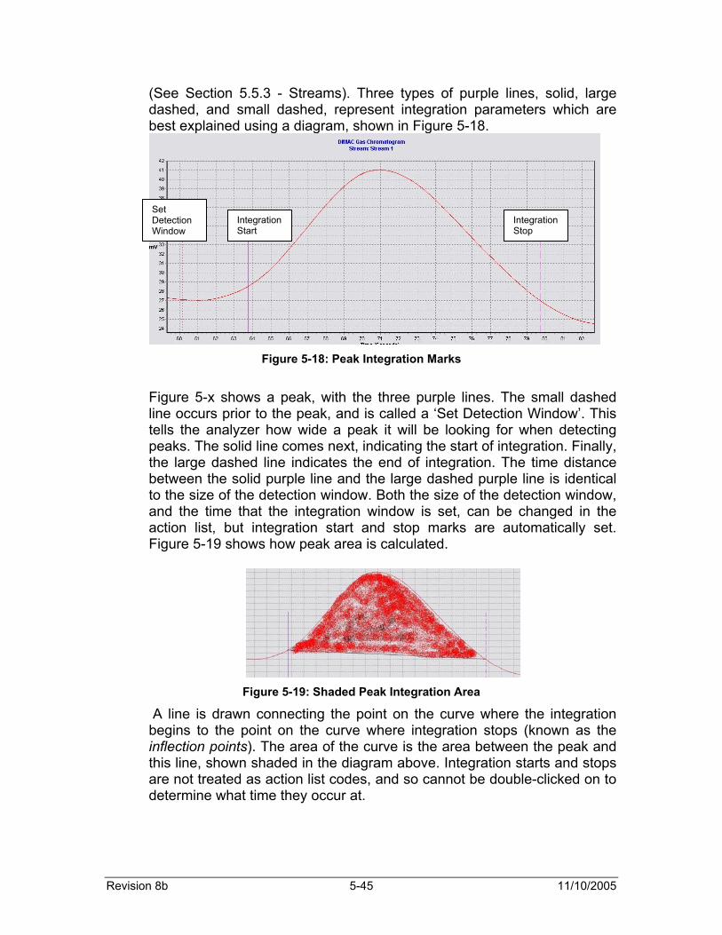
(See Section 5.5.3 - Streams). Three types of purple lines, solid, large dashed, and small dashed, represent integration parameters which are best explained using a diagram, shown in Figure 5-18.
Figure 5-18: Peak Integration Marks
Figure 5-x shows a peak, with the three purple lines. The small dashed line occurs prior to the peak, and is called a ‘Set Detection Window’. This tells the analyzer how wide a peak it will be looking for when detecting peaks. The solid line comes next, indicating the start of integration. Finally, the large dashed line indicates the end of integration. The time distance between the solid purple line and the large dashed purple line is identical to the size of the detection window. Both the size of the detection window, and the time that the integration window is set, can be changed in the action list, but integration start and stop marks are automatically set. Figure 5-19 shows how peak area is calculated.
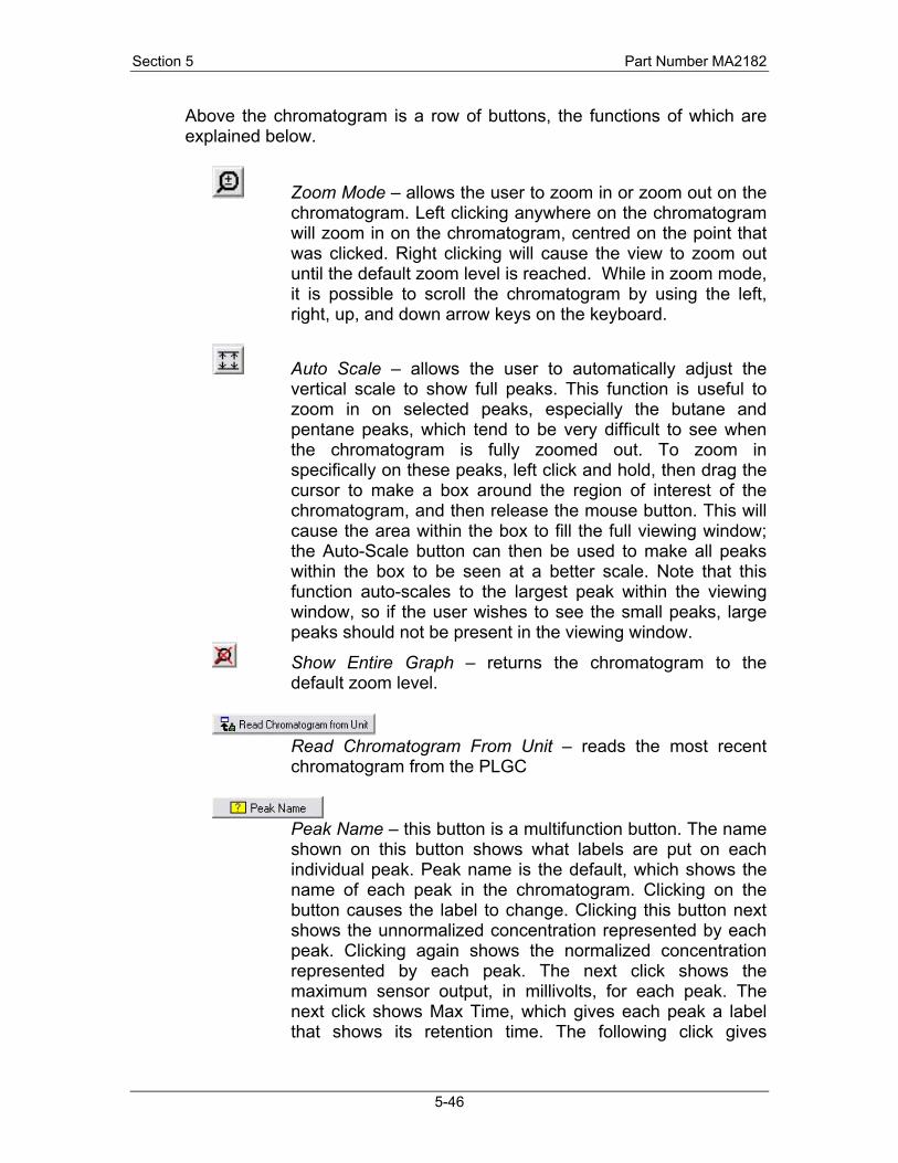
Figure 5-19: Shaded Peak Integration Area
A line is drawn connecting the point on the curve where the integration begins to the point on the curve where integration stops (known as the inflection points). The area of the curve is the area between the peak and this line, shown shaded in the diagram above. Integration starts and stops are not treated as action list codes, and so cannot be double-clicked on to determine what time they occur at.
Set Detection Window
Integration Start
Integration Stop
Section 5 Part Number MA2182
5-46
Above the chromatogram is a row of buttons, the functions of which are explained below.
Zoom Mode – allows the user to zoom in or zoom out on the chromatogram. Left clicking anywhere on the chromatogram will zoom in on the chromatogram, centred on the point that was clicked. Right clicking will cause the view to zoom out until the default zoom level is reached. While in zoom mode, it is possible to scroll the chromatogram by using the left, right, up, and down arrow keys on the keyboard.
Auto Scale – allows the user to automatically adjust the vertical scale to show full peaks. This function is useful to zoom in on selected peaks, especially the butane and pentane peaks, which tend to be very difficult to see when the chromatogram is fully zoomed out. To zoom in specifically on these peaks, left click and hold, then drag the cursor to make a box around the region of interest of the chromatogram, and then release the mouse button. This will cause the area within the box to fill the full viewing window; the Auto-Scale button can then be used to make all peaks within the box to be seen at a better scale. Note that this function auto-scales to the largest peak within the viewing window, so if the user wishes to see the small peaks, large peaks should not be present in the viewing window.
Show Entire Graph – returns the chromatogram to the default zoom level.
Read Chromatogram From Unit – reads the most recent chromatogram from the PLGC
Peak Name – this button is a multifunction button. The name shown on this button shows what labels are put on each individual peak. Peak name is the default, which shows the name of each peak in the chromatogram. Clicking on the button causes the label to change. Clicking this button next shows the unnormalized concentration represented by each peak. Clicking again shows the normalized concentration represented by each peak. The next click shows the maximum sensor output, in millivolts, for each peak. The next click shows Max Time, which gives each peak a label that shows its retention time. The following click gives
Revision 8b 5-47 11/10/2005
Corrected Area, which shows the raw area underneath each peak. Clicking once more gives Off, which removes all labels from the peaks. One more peak will return to Peak Name.
First Peak – clicking this button will immediately show a correctly zoomed view of the first integrated and named peak, regardless of what zoom mode the window is currently in.
Next Peak – clicking this button will show a correctly zoomed
view of the next integrated peak. Continuing to click this button will show zoomed views of all integrated peaks in the chromatogram. This button is useful to see the peak shapes for all peaks in the chromatogram.
Previous Peak – clicking this button will go backwards
through zoomed views of all peaks in the chromatogram.
Last Peak – clicking this button will show a correctly zoomed view of the last integrated peak in the chromatogram.
Autostore All Chromatograms – clicking this button will cause the analyzer to store all subsequent chromatograms in a user-selected directory on the connected PC with a user selected root name. For example, if the user chose the name ‘test’ for the chromatograms, an example filename would be ‘test(Stream 01)001.cgr’. The name in brackets tells which stream was being analyzed for each chromatogram, while the 001 is a sequence number that rises in increments of 1 from whenever the autostorage began. The sequence number starts at 1 for each stream. Please note that auto-storing of chromatograms can only occur while the GC is connected to a PC – no storage of previous chromatograms occurs in the PLGC’s onboard memory. Also, note that each chromatogram is anywhere between 500 kilobytes and 1.5 megabytes, so please ensure that adequate storage is available if this function is selected. To disable this function, simply click this button again.
Right-clicking on the chromatogram brings up a pop-up menu with several options.
• Show Entire Graph – undoes all zooms and returns to the default zoom level
• Undo Last Zoom – undoes the effect of the previous zoom • Autoscale – same function as the button described above
Section 5 Part Number MA2182
5-48
• Show Points – shows each individual data point that makes up the chromatogram. The PLGC samples at 60 samples per second, so there are 60 data points for every second of the chromatogram.
• Load from File – allows the user to load a previously saved chromatogram.
• Save to File – allows the user to save the displayed chromatogram to a *.cgm file.
• Export to CSV – allows the user to save the raw data that makes up the chromatogram to a comma-separated values (*.csv) file that can be opened in Microsoft Excel.
• Export to CSV (with codes) – allows the user to save the raw data that makes up the chromatogram to a CSV file, along with action list codes represented in hexadecimal format. This function is of little use to the normal user, but is useful to Galvanic programmers for debugging purposes should there be problems with a user’s analyzer.
• Print – allows the user to print the displayed chromatogram. • Copy to clipboard – allows the user to copy the chromatogram
image to the clipboard to paste into another application, such as Microsoft Word.
• Update all Response Factors – a response factor is a factor that the peak area for each identified peak is multiplied by to get a concentration value for each component in the gas stream. The response factors are found in the Component Table (See Section 5.5.2). This function allows the user to do a quick calibration based on the displayed chromatogram, as it will update all response factors in the component table based on the peak areas in the chromatogram and the calibration gas values in the Component Table. IMPORTANT: This function MUST only be used if the analyzer is running on calibration gas, and should not be used as a replacement for a proper calibration, as it is based on only a single analysis, and does not recalculate retention times as a true calibration cycle does (for more on Calibrations, see section 5.5.3 – Streams).
• Display Extended Info – displays information about the raw data for the displayed chromatogram. Useful for debugging purposes only.
• Preferences – allows the user to configure the chromatogram display
o Show Action List Codes – toggles action list markers (not integration start/stop marks) on/off.
o Show Inflection Points – toggles integration start/stop markers on/off.
o Set Trace Colour – allows the user to change the colour of the chromatogram
o Set Background Colour – allows the user to change the colour of the background
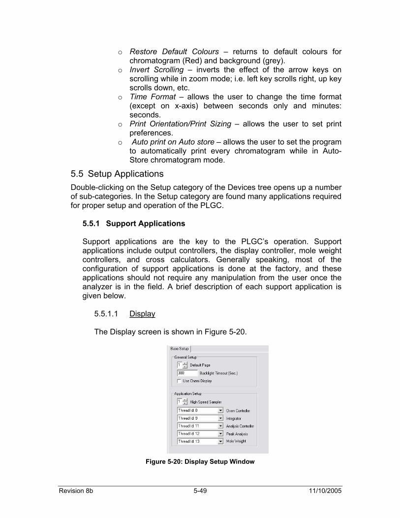
Revision 8b 5-49 11/10/2005
o Restore Default Colours – returns to default colours for chromatogram (Red) and background (grey).
o Invert Scrolling – inverts the effect of the arrow keys on scrolling while in zoom mode; i.e. left key scrolls right, up key scrolls down, etc.
o Time Format – allows the user to change the time format (except on x-axis) between seconds only and minutes: seconds.
o Print Orientation/Print Sizing – allows the user to set print preferences.
o Auto print on Auto store – allows the user to set the program to automatically print every chromatogram while in Auto-Store chromatogram mode.
5.5 Setup Applications Double-clicking on the Setup category of the Devices tree opens up a number of sub-categories. In the Setup category are found many applications required for proper setup and operation of the PLGC.
5.5.1 Support Applications Support applications are the key to the PLGC’s operation. Support applications include output controllers, the display controller, mole weight controllers, and cross calculators. Generally speaking, most of the configuration of support applications is done at the factory, and these applications should not require any manipulation from the user once the analyzer is in the field. A brief description of each support application is given below.
5.5.1.1 Display The Display screen is shown in Figure 5-20.
Figure 5-20: Display Setup Window

Section 5 Part Number MA2182
5-50
The Display screen is used to configure the analyzer’s LCD display. It tells the analyzer what processes it should use to output data – these are seen in the various thread IDs that are shown in the pull down menus. None of the settings in the Display screen should be changed by a user without first consulting Galvanic service staff.
5.5.1.2 Output Controllers
Output controllers are applications that are used to configure the outputs from the PLGC, namely the heater output control that is used to control the temperature in the Column Oven, and the analog outputs that are used to output data in 4-20 milliamp format. In total, most PLGCs are configured from the factory with 5 output controllers – one Oven PID controller, and 4 analog output controllers.
5.5.1.2.1 Oven Controller PID The Oven Controller PID screen is shown in Figure 5-21.
Figure 5-21: Oven PID Controller
The purpose of this application is to control the temperature in the column oven as close to a set value as possible at all times. As the repeatability of the analyzer is dependent on stable temperature control in the column oven, this application is very important to normal operation of the analyzer. Changing the oven temperature
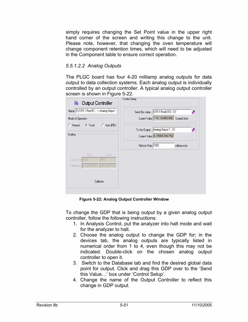
Revision 8b 5-51 11/10/2005
simply requires changing the Set Point value in the upper right hand corner of the screen and writing this change to the unit. Please note, however, that changing the oven temperature will change component retention times, which will need to be adjusted in the Component table to ensure correct operation.
5.5.1.2.2 Analog Outputs The PLGC board has four 4-20 milliamp analog outputs for data output to data collection systems. Each analog output is individually controlled by an output controller. A typical analog output controller screen is shown in Figure 5-22.
Figure 5-22: Analog Output Controller Window
To change the GDP that is being output by a given analog output controller, follow the following instructions:
1. In Analysis Control, put the analyzer into halt mode and wait for the analyzer to halt.
2. Choose the analog output to change the GDP for; in the devices tab, the analog outputs are typically listed in numerical order from 1 to 4, even though this may not be indicated. Double-click on the chosen analog output controller to open it.
3. Switch to the Database tab and find the desired global data point for output. Click and drag this GDP over to the ‘Send this Value…’ box under ‘Control Setup’.
4. Change the name of the Output Controller to reflect this change in GDP output.

Section 5 Part Number MA2182
5-52
5. Determine the correct range for the given GDP. Typical ranges for individual components range from 0-2% to 0-100%, while specific gravity tends to range from 0 to 2, and heating value tends to range from 1000 to 1200 BTU.
6. To change the scale of the output controller, click on ‘Calibrate’ in the ‘Scaling’ box – the text boxes within the ‘Scaling’ box will no longer be greyed out. Enter the correct range into the two boxes to the right of ‘Scale (EU’, with the lower end of the range going under ‘Zero’, and the higher end of the range going under ‘Span’.
7. Write these changes to the unit. 8. Click on the word ‘Calibrate’ to re-grey out the boxes, then
read data from unit to ensure that the change has been successful.
9. Un-halt the analyzer and begin analyses as normal.
For more information about the various fields in the Output Controller windows, it is possible to right-click on any white text input field in the Output Controller windows and choose the ‘What’s This?’ option. This will give more information about what each field is, and links to an in-depth PLGC Help file.
5.5.1.3 Mole Weight Calculators A mole weight calculator is an application that calculates a certain value for a complete gas stream based on the composition of that gas stream. An example of a mole weight calculator is shown in Figure 5-23.
Figure 5-23: Mole Weight Calculator Window
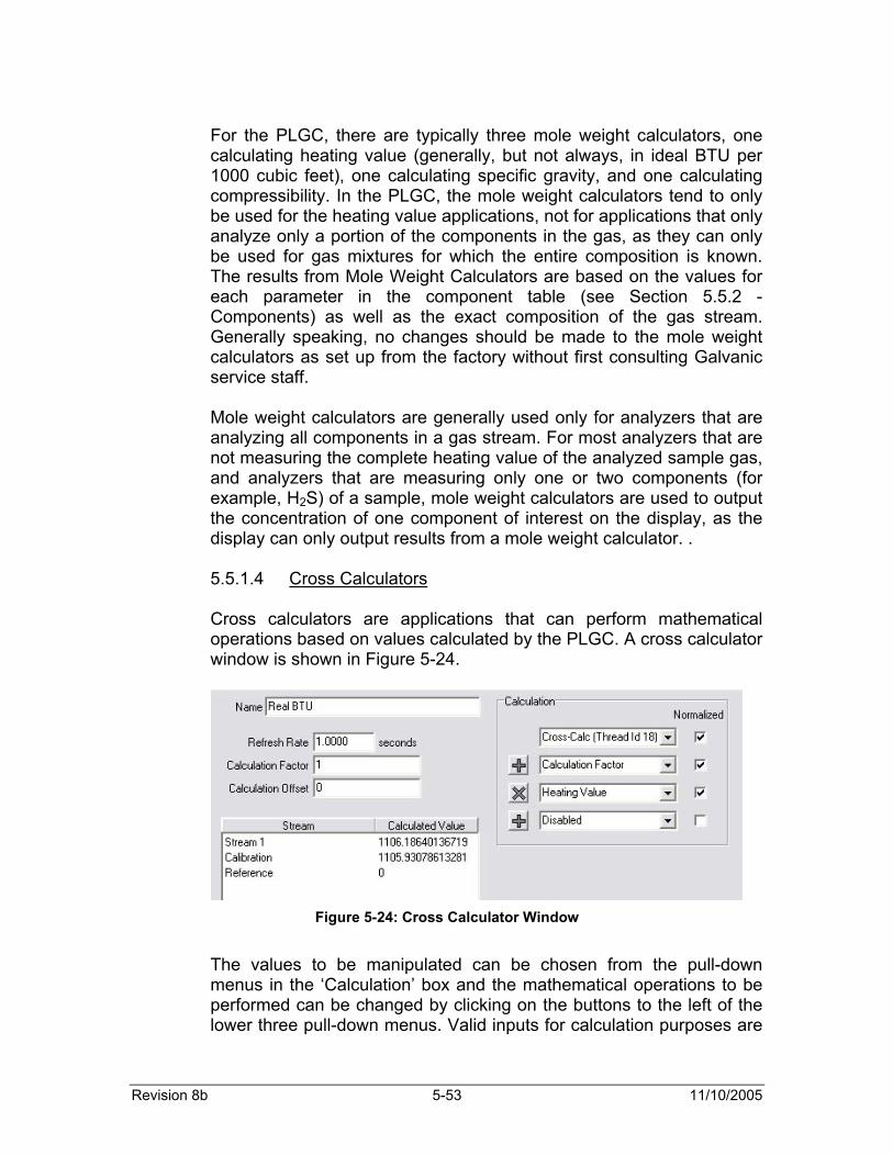
Revision 8b 5-53 11/10/2005
For the PLGC, there are typically three mole weight calculators, one calculating heating value (generally, but not always, in ideal BTU per 1000 cubic feet), one calculating specific gravity, and one calculating compressibility. In the PLGC, the mole weight calculators tend to only be used for the heating value applications, not for applications that only analyze only a portion of the components in the gas, as they can only be used for gas mixtures for which the entire composition is known. The results from Mole Weight Calculators are based on the values for each parameter in the component table (see Section 5.5.2 - Components) as well as the exact composition of the gas stream. Generally speaking, no changes should be made to the mole weight calculators as set up from the factory without first consulting Galvanic service staff. Mole weight calculators are generally used only for analyzers that are analyzing all components in a gas stream. For most analyzers that are not measuring the complete heating value of the analyzed sample gas, and analyzers that are measuring only one or two components (for example, H2S) of a sample, mole weight calculators are used to output the concentration of one component of interest on the display, as the display can only output results from a mole weight calculator. .
5.5.1.4 Cross Calculators Cross calculators are applications that can perform mathematical operations based on values calculated by the PLGC. A cross calculator window is shown in Figure 5-24.
Figure 5-24: Cross Calculator Window
The values to be manipulated can be chosen from the pull-down menus in the ‘Calculation’ box and the mathematical operations to be performed can be changed by clicking on the buttons to the left of the lower three pull-down menus. Valid inputs for calculation purposes are

Section 5 Part Number MA2182
5-54
component concentrations, the calculated values from mole weight calculators, and the calculated values from previous cross calculators. Cross calculators are most commonly used to calculate real BTU values from ideal BTU values, as well as Wobbe index for a gas stream. Detailed instructions as to how to add these calculations to a PLGC that does not currently have these calculations installed can be found in Sections 5.6.2 and 5.6.3.
5.5.2 Components The component table is the most important input area in the entire PLGC. The component table stores data about the names, calibration gas values, retention times, response factors, heating values, specific gravities, and compressibilities for every component that may be present in the analyzed gas stream. A sample component table is shown in Figure 5-25.
Figure 5-25: Component Table
A brief explanation of each column is provided here:
• Calibration Gas Value – the concentration of each component found in the calibration gas cylinder. These values are taken off the certificate or paperwork included with the calibration cylinder.
• Response Factor – a multiplication factor that converts a raw peak area into a concentration value. See Appendix B for more information about how response factors are calculated.
• Retention Time – the time, in seconds, at which the given component elutes from the column and reaches the detector. Peaks in a chromatogram are identified on the basis of their
Revision 8b 5-55 11/10/2005
retention times, as each component has its own unique retention time.
• Retention Time Deviation – the amount of time, in seconds, that a peak is allowed to deviate from the set retention time for a given component and still be identified as that component. For example, in the sample component table, methane has a retention time of 26.95 seconds, and a deviation of 5 seconds. This means that a peak with a retention time anywhere between 21.95 seconds and 31.95 seconds will be identified as methane. Generally speaking, peaks that elute early in the analysis will have small retention time deviations (± 5 seconds or less), while later peaks will have larger deviations (± 10 seconds or more).
• Heating Value – the calorific value of each component in the gas. These values are obtained from some accepted standard (GPA 2145, AGA 2145, ISO 6976 are the most common). Some typical values for all components are found in the table in Appendix C. The typical configuration for the PLGC has the heating value given as ideal dry BTU per 1000 cubic feet, at a pressure of 14.696psi, although figures for other conditions are available at customer request.
• Specific Gravity – the density of each component, relative to air, which has a specific gravity of 1.
• Compressibility – the deviation of the volume of a given component from the volume of that component were it an ideal gas.
Below the table is a box that is entitled Calibration Gas results. It has four boxes that show summed information for the calibration gas.
• Component Total – shows the sum of the concentrations of all components in the gas. If this sum is not 100, normalization cannot be used in calculations. If this sum is not 100, but the calibration gas is supposed to have a sum of 100%, please check all entered concentrations for errors.
• Heating Value – shows the heating value of a gas with component concentrations as entered in the table. Reference runs (see section 5.x) using a calibration gas of this composition should produce a value close to this heating value if the analyzer is correctly calibrated.
• Specific Gravity – shows the specific gravity of the total calibration gas.
• Compressibility – shows the compressibility of the total calibration gas.
Changing component values for concentration, heating value, specific gravity, or compressibility is simple. Left click on the cell in the table that needs to be changed, and then type in the new value. If changing the
Section 5 Part Number MA2182
5-56
entire calibration gas concentration values, ensure that they add up to 100%. When all changes are made, write the new table to the unit. Right-clicking on the white field surrounding the Components table brings up an option list, whose options are described below:
• Auto size Columns – resizes the columns to fit the contents in the columns
• Add New Component – allows the user to add another row to the table to enter data for a new component in the gas stream. If a new component is added, remember to write changes to the unit.
• Add New Column – allows the user to add another column to the table that can be used in a mole weight calculator. For example, if the user wishes to calculate both dry and saturated heating value, he or she could add another column containing saturated heating value data. The numerical values for this column must be obtained from a recognized standard, such as GPA 2145-03.
• Delete Unused Columns – deletes any column whose contents are solely zeroes. If this option is chosen, and there are unused columns in the component table, remember to write these changes to the unit.
• Print Preview – previews how a print-out of the component table would look.
• Print – allows the user to print the component table. • Load Configuration File – allows the user to load a saved
component table from a Galvanic proprietary (*.dc101a) file. This option is useful if incorrect changes are made to the PLGC and the original configuration needs to be recovered.
• Save Configuration File – saves the current component table to a directory of the user’s choice in Galvanic proprietary (*.dc101a) format.
• Save as CSV – saves the current component table as a comma-separated value (*.csv) file for opening in a spreadsheet program such as Microsoft Excel.
• Save as XLS – saves the current component table as a Microsoft Excel (*.xls) spreadsheet file.
• Copy Image to Clipboard – copies the current Component table, including the boxes showing heating value, specific gravity, and compressibility, as an image to the clipboard, so that it can be pasted into another application, such as Microsoft Word.
In addition, if the user left-clicks on a single component to highlight that row in the table, right clicking the highlighted row brings up a menu with all of the options described above, plus two more options of interest.
• Rename Selected Component – allows the user to rename any component in the table.
Revision 8b 5-57 11/10/2005
• Delete Selected Component – allows the user to delete the selected component.
Misusing these options has the potential to adversely affect the operation of the PLGC, so the use of these options should only be undertaken after consultation with Galvanic service staff. The data in the table can also be sorted in ascending or descending order of the numerical values in the columns. To sort the table, left-click once on the column heading of the desired column, and the table will be sorted in ascending numerical order based on the data in that column. To sort the column in descending order, left-click again on the column header. By default, data in the Components table is sorted in ascending order based on retention times. Note that the heating value, specific gravity, and compressibility for the stream will not be displayed correctly for most applications other than complete heating value analysis, such as PLGCs configured to analyze H2S only, or H2S in conjunction with a few other components, not including all of the components in the stream.
5.5.3 Streams
The stream setup window is the window that shows how each of the various streams to be analyzed by the PLGC is setup. This tells the analyzer which solenoids to actuate for a given stream, what GDPs should be written to for each stream, and what type of stream it is. A typical stream setup window is shown in Figure 5-26. The three types of streams defined for the PLGC are normal, calibration, and reference.
• Normal – a normal stream is a stream that is used to analyze sample gas, giving results that are useful for plant operations.
• Calibration – a calibration stream is a stream that is used to calibrate the analyzer, giving new response factors and retention times for all components, to ensure that it gives accurate results when operating on a normal stream.
• Reference – a reference stream is a stream that is used to check the calibration status of a PLGC. As the heating value content of a calibration gas is a known value – the heating value for the calibration gas is shown at the bottom of the Components window – if the heating value obtained on the reference run does not closely match this known value, a calibration is necessary.

Section 5 Part Number MA2182
5-58
Figure 5-26: Streams Set up Window
The stream type is selected using the pull-down menu in the top left corner of the Streams setup window. Below this menu is a box called ‘Minimum Purge Time’. The Minimum Purge Time is the minimum amount of time a new stream must pass through the sample loop in the column oven prior to starting analysis of this stream. At the bottom of the screen are tabs that allow the user to switch between the configurations for the streams that are installed on the PLGC. All PLGCs will have a minimum of 3 streams – at least one sample stream, a calibration stream, and a reference stream. A stream can be renamed by right-clicking on the tab at the bottom of the screen and selecting ‘Rename Current Stream’. Note that changing the name of a stream requires that this information be written to the analyzer.
5.5.3.1 Stream Path
The stream path is a window that shows which control points are actuated for a given stream. Generally speaking, each individual stream will be controlled by its own solenoid, with calibration and reference streams usually controlled by the same solenoid.

Revision 8b 5-59 11/10/2005
In Figure 5-26, an analyzer with 4 sample streams plus a reference and a calibration stream is shown. In the Stream Path window for Stream 1 there are four solenoids shown – the Calibration solenoid, and Solenoids 1-4. There are a total of 8 solenoid drivers on the PLGC Motherboard, plus the Calibration Solenoid, which means that a total of 8 streams, plus Reference and Calibration, can be analyzed by the PLGC. The Control Points for stream control come from the Database tab, under ‘Global Data Points I/O Controls’, and are simply dragged from the database window into the white box in the Stream Path window. Next to each control point shown in the Stream Path window is a check box. If there is a checkmark in this box, it means that the given control point will be energized for that stream. For example, in Figure 5-26, the Stream 1 Stream Path shows that Solenoid 1 is energized, while the Calibration Solenoid, and Solenoids 2,3, and 4 are de-energized. The reason that all solenoids are shown in each stream is because control points stay in a given state until they are told specifically to change state. That is to say, if Solenoid 1 is turned on for Stream 1, it will stay on unless the subsequent streams tell it explicitly to shut off. Thus, each individual stream is configured to have its solenoid (or other control point) turn on, and all other solenoids to turn off, to ensure that only the solenoid or control point that controls a given stream is on, and all other control points are off, when that stream is being analyzed. Therefore, if adding a new control point for a given stream, ensure that this control point is added to the Stream Path of all the other streams set up on the analyzer to ensure this new control point is explicitly shut off in all other streams. For more detailed information on Stream Paths from the PLGC Help File, right click anywhere on the white field under Stream Paths, and choose the ‘What’s This?’ option. 5.5.3.2 Stream Components
The Stream Components field is where GDPs are associated with components or component table columns. This tells the software which GDPs are associated with which numerical values, so setting up the stream components correctly is essential to making the PLGC output useable data.
The Component Table column means that the value associated with the given GDP is an output of either a mole weight calculator or a cross calculator. For this to produce correct results, if the mole weight calculator or cross calculator is set up to use normalized values, the
Section 5 Part Number MA2182
5-60
‘Normalize’ checkbox next to each GDP must also be checked, otherwise the GDP will simply contain garbage values. The Component column associates a calculated concentration value with the given global data point. If the Normalized checkbox is checked, this will associate the normalized concentration value for a given component with this GDP, whereas if the normalized checkbox is not checked, this will associate the un-normalized concentration value with the GDP. To add a new global data point to the stream component field, drag the desired GDP from the database into the Stream Components field. Choose the desired component table column (if the new component is a calculated output from either a mole weight calculator or a cross calculator) or the desired component to associate with this new global data point. To change the Component Table column or Component associated with a given GDP, first left-click on the cell of the table to be changed. Left-clicking again will cause a pop-up menu to appear giving all the possible options for the Component or Component Table column. To ensure that normalized data is associated with a given GDP, check the normalized check box. To delete a global data point from a stream, right click on the component to be deleted, and chose ‘Delete Row’, then write the changes to the analyzer. For analyzers that are not measuring all components, ensure that the Normalized checkboxes for the components are not checked; otherwise the results entered into the GDPs will be invalid. Note the GDP names in the Database have Stream prefixes that tell the user which stream to associate the GDPs with. For example, stream 1 GDPs will usually be prefixed with STR 1, calibration stream GDPs will be prefixed CAL, and reference stream GDPs will be prefixed REF. Ensure that the GDPs are correctly associated with their streams. Finally, it is important to make certain that each individual GDP is only associated with a single stream – to have the same GDP associated with more than one stream will cause invalid results to be stored in a given GDP. For more information regarding the Stream Components setup, right-click anywhere within the Stream Components field and select ‘What’s This?’. This will give a brief description of the Stream Components field, and provide a link to the PLGC in-depth help file. Right-clicking anywhere on the Stream Components field also allows the user to save a stream to a file or load a stream from a file. Note that Stream configuration files (*.dcsm files) only store data for
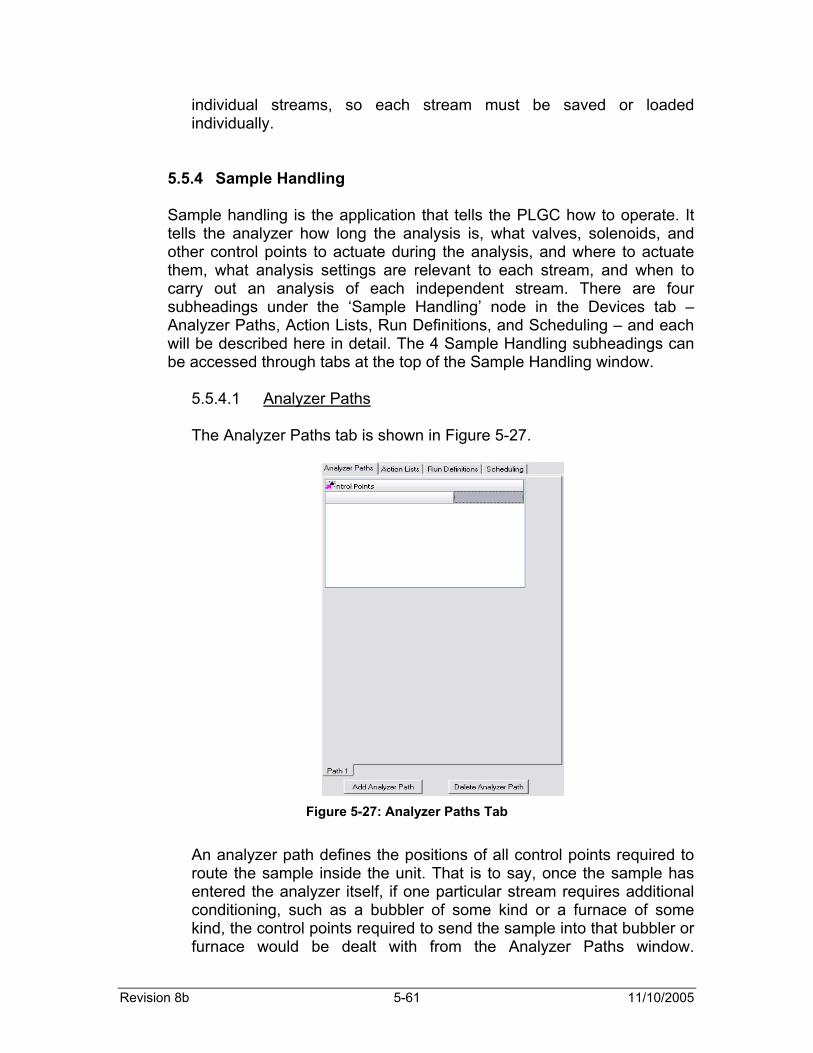
Revision 8b 5-61 11/10/2005
individual streams, so each stream must be saved or loaded individually.
5.5.4 Sample Handling Sample handling is the application that tells the PLGC how to operate. It tells the analyzer how long the analysis is, what valves, solenoids, and other control points to actuate during the analysis, and where to actuate them, what analysis settings are relevant to each stream, and when to carry out an analysis of each independent stream. There are four subheadings under the ‘Sample Handling’ node in the Devices tab – Analyzer Paths, Action Lists, Run Definitions, and Scheduling – and each will be described here in detail. The 4 Sample Handling subheadings can be accessed through tabs at the top of the Sample Handling window.
5.5.4.1 Analyzer Paths The Analyzer Paths tab is shown in Figure 5-27.
Figure 5-27: Analyzer Paths Tab
An analyzer path defines the positions of all control points required to route the sample inside the unit. That is to say, once the sample has entered the analyzer itself, if one particular stream requires additional conditioning, such as a bubbler of some kind or a furnace of some kind, the control points required to send the sample into that bubbler or furnace would be dealt with from the Analyzer Paths window.
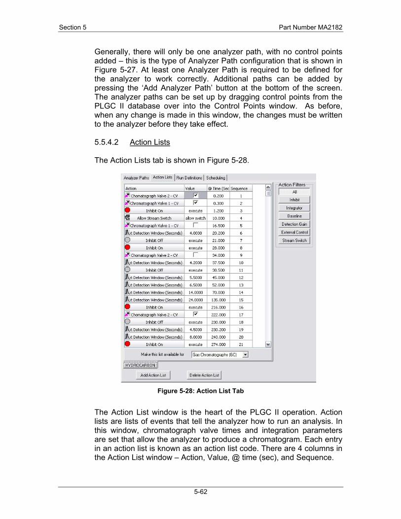
Section 5 Part Number MA2182
5-62
Generally, there will only be one analyzer path, with no control points added – this is the type of Analyzer Path configuration that is shown in Figure 5-27. At least one Analyzer Path is required to be defined for the analyzer to work correctly. Additional paths can be added by pressing the ‘Add Analyzer Path’ button at the bottom of the screen. The analyzer paths can be set up by dragging control points from the PLGC II database over into the Control Points window. As before, when any change is made in this window, the changes must be written to the analyzer before they take effect. 5.5.4.2 Action Lists
The Action Lists tab is shown in Figure 5-28.
Figure 5-28: Action List Tab
The Action List window is the heart of the PLGC II operation. Action lists are lists of events that tell the analyzer how to run an analysis. In this window, chromatograph valve times and integration parameters are set that allow the analyzer to produce a chromatogram. Each entry in an action list is known as an action list code. There are 4 columns in the Action List window – Action, Value, @ time (sec), and Sequence.
Revision 8b 5-63 11/10/2005
• Action – describes what type of action each action list code is. There are several types of action list code, described in detail below:
o External Controls – an external control tells the analyzer to trigger a valve, a solenoid, or a relay at a given time during the analysis. Any Action List Code with a pink arrow icon in front of it ( ) is an external control. Generally speaking, chromatograph valves (1 for a 12 minute analysis and for H2S analysis, 2 for a high speed heating value analysis) are the only external controls in an action list.
o Allow stream switch – allows the analyzer to switch streams during an analysis. This allows the analyzer to purge the sample system with the upcoming stream for a longer period of time prior to the analysis, so this is typically placed quite early in an analysis. The stream that is switched to is defined either manually in the Analysis Control window, or automatically in the Scheduling section of Sample Handling (see Section 5.5.4.4).
o Inhibit On/Off – turns integration inhibition on or off. When inhibit is turned on, the PLGC will not integrate any peaks until an inhibit off action list code is triggered.
o Set Detection Window (Seconds) – allows the user to change the width of the integration window (See Section 5.4.5 – Peak Integration). The wider the peak in the chromatogram, the wider the Detection Window required for accuracy and repeatability. As a result, several ‘Set Detection Window’ actions are required during an analysis, because not all peaks in a chromatogram have the same width.
• Value – the value column can show one of three things; a number, a check box, or ‘execute’. Check boxes are associated with control points. If a control point, normally a chromatograph valve, has its check box checked, that means that the control point is being turned on, and if the check box is unchecked, the control point is being turned off. Execute is used for inhibit events, as it simply states that the inhibit on or off is being carried out. The numbers in this column show are associated with ‘Set Detection Windows’, and show the width, in seconds, of each Detection Window being set.
• @ Time (seconds) – shows the time, in seconds, during an analysis where an event occurs.
• Sequence – shows the order in which events occur, from 1 to the highest number in the sequence.

Section 5 Part Number MA2182
5-64
Some streams may require a different action list to correctly carry out an analysis, for example if the stream compositions vary significantly from stream to stream. To add another action list, click on the ‘Add Action List’ button at the bottom left of the Action Lists window, and a pop-up window will appear asking for a name for the new action list. Enter a name for the list, press OK, and a new blank action list will be created. Action lists can be renamed later by right clicking on the tab where the name is displayed and selecting “Rename current Action List” from the pop-up menu. Right-clicking on the white field of the action list brings up a pop-up menu with the following options.
• What’s This? – provides access to the help file regarding Action Lists, including an in-depth examination of how to add actions to an action list.
• Add New Action – allows the user to add a new action to the action list. See Section 5.5.4.2.1 for more information as to how to add actions to an action list.
• Print – prints the action list to the default printer. • Load Sample Handling Configuration from File – loads a pre-
saved sample handling configuration file (*.dcsh). Note that this will replace ALL configurations under the Sample Handling heading – analyzer paths, action lists, run definitions, and scheduling.
• Save Sample Handling Configuration to File – saves the Sample Handling configuration – analyzer paths, action lists, run definitions, and scheduling – to a *.dcsh file.
On the right hand side of the Action List window is a section with several buttons called ‘Action Filters’. By default, ‘All’ is selected, and this will show all the action list codes in the action list. The other buttons filter the list to show only specific types of action list codes.
• Inhibit – shows only Inhibit On/Off events. • Detection Gain – shows only the Set Detection Window events. • External Control – shows only external control events, such as
chromatograph valves, relays, and solenoids. • Stream Switch – shows only stream switch events.
IMPORTANT: Do NOT press the ‘Write Changes to Unit’ button when any of these filters other than the ‘All’ filter is selected. Writing changes to unit with an Action filter selected will wipe out the entire action list in the unit and cause it to no longer function correctly.
5.5.4.2.1 Adding Actions to an Action List
Two types of actions can be added to the action list: standard actions and external controls. Standard actions are actions such as integration parameters and inhibits. To add a standard action to an
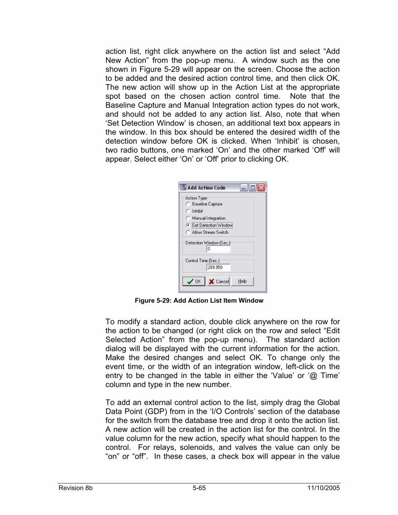
Revision 8b 5-65 11/10/2005
action list, right click anywhere on the action list and select “Add New Action” from the pop-up menu. A window such as the one shown in Figure 5-29 will appear on the screen. Choose the action to be added and the desired action control time, and then click OK. The new action will show up in the Action List at the appropriate spot based on the chosen action control time. Note that the Baseline Capture and Manual Integration action types do not work, and should not be added to any action list. Also, note that when ‘Set Detection Window’ is chosen, an additional text box appears in the window. In this box should be entered the desired width of the detection window before OK is clicked. When ‘Inhibit’ is chosen, two radio buttons, one marked ‘On’ and the other marked ‘Off’ will appear. Select either ‘On’ or ‘Off’ prior to clicking OK.
Figure 5-29: Add Action List Item Window
To modify a standard action, double click anywhere on the row for the action to be changed (or right click on the row and select “Edit Selected Action” from the pop-up menu). The standard action dialog will be displayed with the current information for the action. Make the desired changes and select OK. To change only the event time, or the width of an integration window, left-click on the entry to be changed in the table in either the ‘Value’ or ‘@ Time’ column and type in the new number. To add an external control action to the list, simply drag the Global Data Point (GDP) from in the ‘I/O Controls’ section of the database for the switch from the database tree and drop it onto the action list. A new action will be created in the action list for the control. In the value column for the new action, specify what should happen to the control. For relays, solenoids, and valves the value can only be “on” or “off”. In these cases, a check box will appear in the value
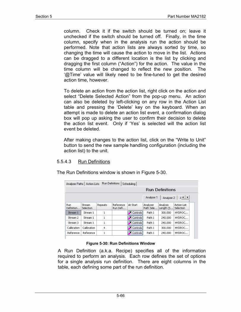
Section 5 Part Number MA2182
5-66
column. Check it if the switch should be turned on; leave it unchecked if the switch should be turned off. Finally, in the time column, specify when in the analysis run the action should be performed. Note that action lists are always sorted by time, so changing the time will cause the action to move in the list. Actions can be dragged to a different location is the list by clicking and dragging the first column (“Action”) for the action. The value in the time column will be changed to reflect the new position. The ‘@Time’ value will likely need to be fine-tuned to get the desired action time, however. To delete an action from the action list, right click on the action and select “Delete Selected Action” from the pop-up menu. An action can also be deleted by left-clicking on any row in the Action List table and pressing the ‘Delete’ key on the keyboard. When an attempt is made to delete an action list event, a confirmation dialog box will pop up asking the user to confirm their decision to delete the action list event. Only if ‘Yes’ is selected will the action list event be deleted. After making changes to the action list, click on the “Write to Unit” button to send the new sample handling configuration (including the action list) to the unit.
5.5.4.3 Run Definitions
The Run Definitions window is shown in Figure 5-30.
Figure 5-30: Run Definitions Window
A Run Definition (a.k.a. Recipe) specifies all of the information required to perform an analysis. Each row defines the set of options for a single analysis run definition. There are eight columns in the table, each defining some part of the run definition.

Revision 8b 5-67 11/10/2005
• Run Definition Name – The name of the run definition will be used on the Scheduling tab (see Section 5.5.4.4) to schedule the analysis to run. The name is also used in the Analysis Control window for manually adding a run definition to the queue. To change the name, simply left-click on the run definition name to be changed and type in the new name.
• Repeats – The number of repeats specifies how many times in a row an analysis should run each time the run definition is scheduled. This is typically 1 for all streams except for Calibration streams, but can be modified as the user sees fit. For Calibration streams, the number of repeats is typically 3 or 4.
• Reference Run – This applies to Calibration run definitions only. If a reference run is selected in a Calibration run definition, the analyzer will automatically carry out a reference run immediately after completing the Calibration run. This is one way to check the validity of the calibration immediately after it is completed, but reference runs can also be scheduled separately in the Scheduling tab.
• At Start – The At Start column allows the user to set up notification that a certain stream is being analyzed. This notification can be either through a specific GDP or an external control such as a relay, which could cause a light in the control room to turn on. Clicking on any cell in the ‘At Start will bring up the dialog box shown in Figure 5-31.
Figure 5-31: At-Start GDP Receiver Dialog Box
If an external control, such as a relay, is dragged from the database into the GDP Receiver, a checkbox will appear in the right-hand column. If this box is checked, this will make the selected control point turn on as soon as the given run definition starts. If a GDP is dragged from the database into the GDP Receiver, the right-hand column will, by default, contain the value 0.00. To make the chosen GDP output a specific value
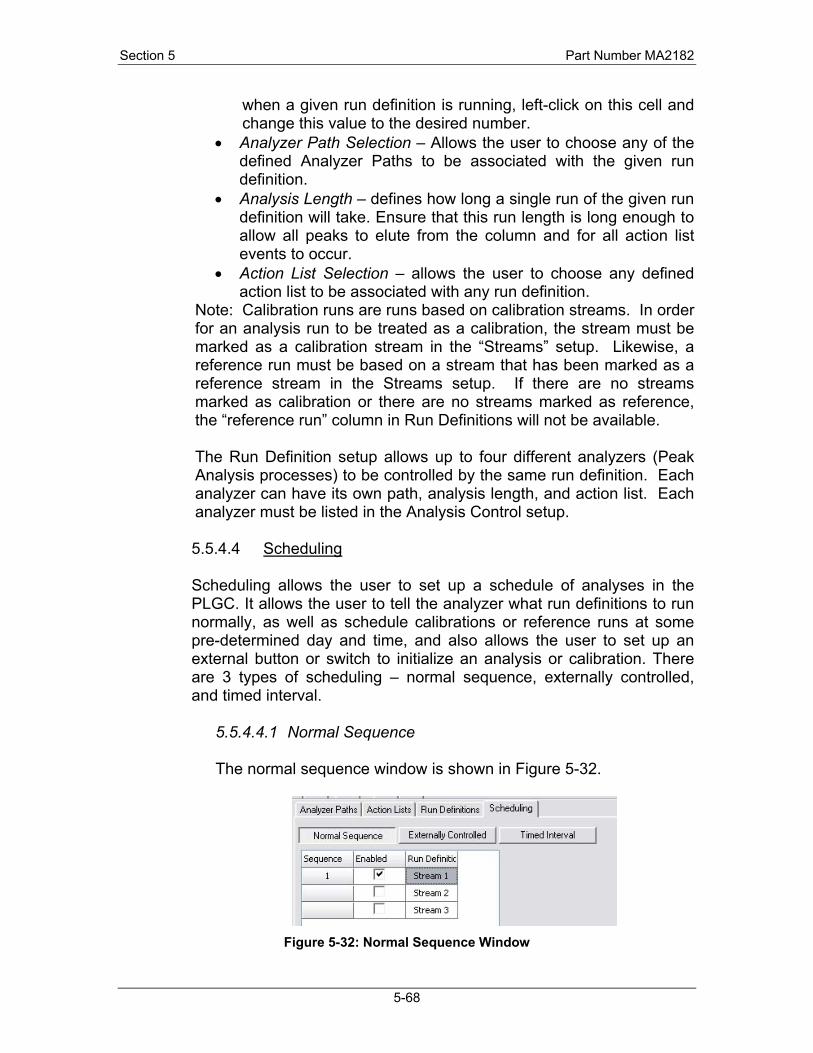
Section 5 Part Number MA2182
5-68
when a given run definition is running, left-click on this cell and change this value to the desired number.
• Analyzer Path Selection – Allows the user to choose any of the defined Analyzer Paths to be associated with the given run definition.
• Analysis Length – defines how long a single run of the given run definition will take. Ensure that this run length is long enough to allow all peaks to elute from the column and for all action list events to occur.
• Action List Selection – allows the user to choose any defined action list to be associated with any run definition.
Note: Calibration runs are runs based on calibration streams. In order for an analysis run to be treated as a calibration, the stream must be marked as a calibration stream in the “Streams” setup. Likewise, a reference run must be based on a stream that has been marked as a reference stream in the Streams setup. If there are no streams marked as calibration or there are no streams marked as reference, the “reference run” column in Run Definitions will not be available.
The Run Definition setup allows up to four different analyzers (Peak Analysis processes) to be controlled by the same run definition. Each analyzer can have its own path, analysis length, and action list. Each analyzer must be listed in the Analysis Control setup. 5.5.4.4 Scheduling
Scheduling allows the user to set up a schedule of analyses in the PLGC. It allows the user to tell the analyzer what run definitions to run normally, as well as schedule calibrations or reference runs at some pre-determined day and time, and also allows the user to set up an external button or switch to initialize an analysis or calibration. There are 3 types of scheduling – normal sequence, externally controlled, and timed interval.
5.5.4.4.1 Normal Sequence
The normal sequence window is shown in Figure 5-32.
Figure 5-32: Normal Sequence Window
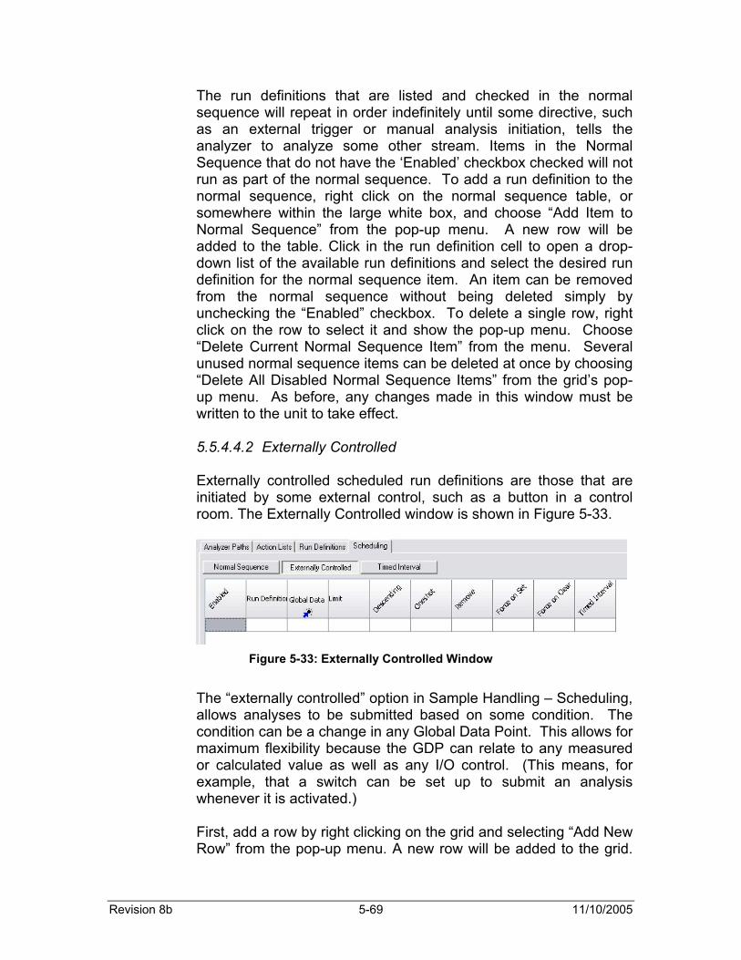
Revision 8b 5-69 11/10/2005
The run definitions that are listed and checked in the normal sequence will repeat in order indefinitely until some directive, such as an external trigger or manual analysis initiation, tells the analyzer to analyze some other stream. Items in the Normal Sequence that do not have the ‘Enabled’ checkbox checked will not run as part of the normal sequence. To add a run definition to the normal sequence, right click on the normal sequence table, or somewhere within the large white box, and choose “Add Item to Normal Sequence” from the pop-up menu. A new row will be added to the table. Click in the run definition cell to open a drop-down list of the available run definitions and select the desired run definition for the normal sequence item. An item can be removed from the normal sequence without being deleted simply by unchecking the “Enabled” checkbox. To delete a single row, right click on the row to select it and show the pop-up menu. Choose “Delete Current Normal Sequence Item” from the menu. Several unused normal sequence items can be deleted at once by choosing “Delete All Disabled Normal Sequence Items” from the grid’s pop-up menu. As before, any changes made in this window must be written to the unit to take effect.
5.5.4.4.2 Externally Controlled
Externally controlled scheduled run definitions are those that are initiated by some external control, such as a button in a control room. The Externally Controlled window is shown in Figure 5-33.
Figure 5-33: Externally Controlled Window
The “externally controlled” option in Sample Handling – Scheduling, allows analyses to be submitted based on some condition. The condition can be a change in any Global Data Point. This allows for maximum flexibility because the GDP can relate to any measured or calculated value as well as any I/O control. (This means, for example, that a switch can be set up to submit an analysis whenever it is activated.)
First, add a row by right clicking on the grid and selecting “Add New Row” from the pop-up menu. A new row will be added to the grid.
Section 5 Part Number MA2182
5-70
Click in the run definition cell to open a drop-down list of the available run definitions. Select a run definition. Next, drag and drop a GDP from the database tab onto the “Global Data Point” cell. If the GDP represents an external control that can only be on or off, such as a discrete input, valve, or solenoid, a checkbox will appear in the “Limit” cell. Check it to indicate that the condition should trigger when it is on, uncheck it to indicate that the condition should trigger when it is off. The most typical use of the externally controlled run definition trigger is for using a button to trigger an analysis, usually a calibration. The button is wired to one of the discrete inputs on the analyzer motherboard, and this discrete input is placed in the externally controlled table. If the GDP represents something that is not on/off, type the trigger value into the “Limit” cell. The analysis will be submitted to the queue whenever the current value of the GDP is greater than or equal to the limit. The other checkboxes can be used to tailor how the condition is handled.
• Descending – Treat the limit as a descending limit. That is, run the analysis when the current value of the GDP is less than the limit.
• Oneshot – Only submit the analysis run to the queue when the current value of the GDP first passes the limit. If ‘Oneshot’ is not checked, the job will be resubmitted to the queue after it finishes for as long as the condition remains true.
• Remove – If this is checked and the condition goes away after the job has been submitted to the queue, but before it has started to run, then the job is removed from the queue.
• Force on Set – If this is checked, the current analysis is interrupted the given run definition analysis is forced to start immediately.
• Force on Clear – If the condition goes away during this analysis, the analysis is aborted.
• Timed Interval – This is used to submit an analysis run only when both the GDP condition is met and a time interval condition is met. When this is checked, this row will also appear on the “Timed Interval” page. The time condition must be set up on that screen (see Section 5.5.4.4.3).
An item can be made inactive without being deleted simply by unchecking the “Enabled” checkbox. To delete an item, right click on the row to select it and show the pop-up menu. Choose “Delete Current Row” from the menu. The externally controlled scheduling setup can be printed by selecting “Print” from the pop-up menu or by clicking on the Print button in the main toolbar while this screen is active. All changes must be written to the unit to take effect.
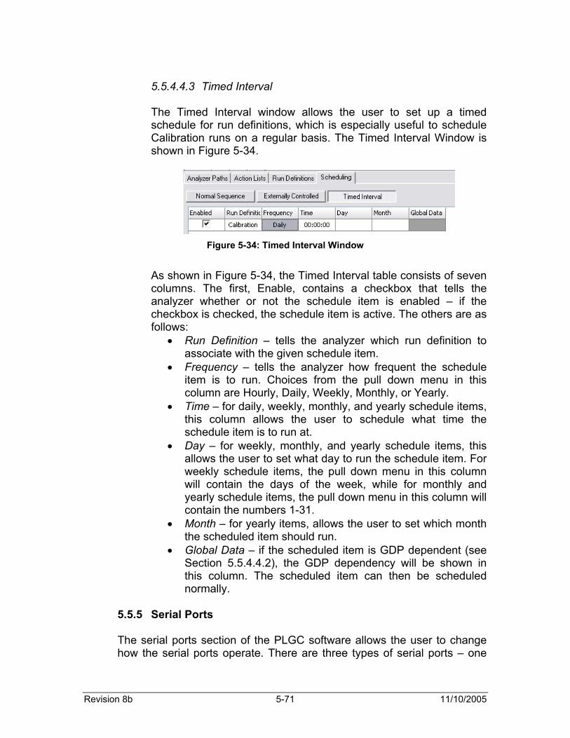
Revision 8b 5-71 11/10/2005
5.5.4.4.3 Timed Interval
The Timed Interval window allows the user to set up a timed schedule for run definitions, which is especially useful to schedule Calibration runs on a regular basis. The Timed Interval Window is shown in Figure 5-34.
Figure 5-34: Timed Interval Window
As shown in Figure 5-34, the Timed Interval table consists of seven columns. The first, Enable, contains a checkbox that tells the analyzer whether or not the schedule item is enabled – if the checkbox is checked, the schedule item is active. The others are as follows:
• Run Definition – tells the analyzer which run definition to associate with the given schedule item.
• Frequency – tells the analyzer how frequent the schedule item is to run. Choices from the pull down menu in this column are Hourly, Daily, Weekly, Monthly, or Yearly.
• Time – for daily, weekly, monthly, and yearly schedule items, this column allows the user to schedule what time the schedule item is to run at.
• Day – for weekly, monthly, and yearly schedule items, this allows the user to set what day to run the schedule item. For weekly schedule items, the pull down menu in this column will contain the days of the week, while for monthly and yearly schedule items, the pull down menu in this column will contain the numbers 1-31.
• Month – for yearly items, allows the user to set which month the scheduled item should run.
• Global Data – if the scheduled item is GDP dependent (see Section 5.5.4.4.2), the GDP dependency will be shown in this column. The scheduled item can then be scheduled normally.
5.5.5 Serial Ports
The serial ports section of the PLGC software allows the user to change how the serial ports operate. There are three types of serial ports – one

Section 5 Part Number MA2182
5-72
RS-232 port on the front door, an isolated RS-232 port on the motherboard, and an RS-485 port, also on the motherboard. An example of a serial port setup window is shown in Figure 5-35.
Figure 5-35: Serial Port Setup Window
The serial port setup window allows the user to configure the speed of the serial connection, as well as other parameters that may be required for the software to correctly communicate with the analyzer. The default settings will work for nearly all standard communications setups, so do not make any changes to these setups except after consultation with Galvanic service staff.
5.5.6 Modbus The PLGC is capable of handling communications in three forms of Modbus – Enron, Modicon 16, and Modicon with Floating Point. Each individual customer will have specific communications requirements, so setting up Modbus is a process that is best done in conjunction with and with the assistance of Galvanic Applied Sciences Inc. Service staff. 5.5.7 Archive Setup
Archive Setup is the section of the software where the user can configure the archives, telling the analyzer what data and Global Data Point values to store in archives for reading in the Archive Reader (Section 5.4.2). The archive setup window is shown in Figure 5-36. The archive setup window is dominated by a table with 8 columns. The last four columns, which reference alarms, do not currently work as the alarm feature for GDPs has not yet been incorporated into the software. The first column simply shows the Item Number, which is just the sequence of the Global Data Points in the archive. The second shows the Global Data Points that will be stored in a given archive. The third is titled Absolute Change Trigger. If the
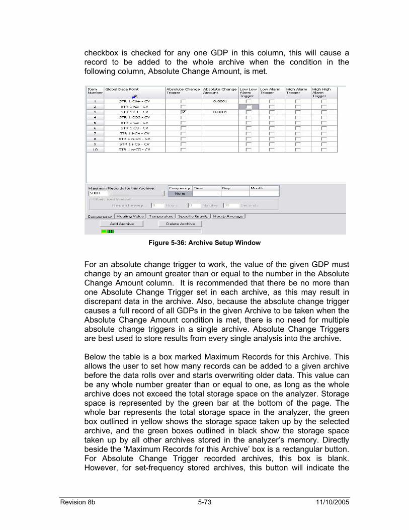
Revision 8b 5-73 11/10/2005
checkbox is checked for any one GDP in this column, this will cause a record to be added to the whole archive when the condition in the following column, Absolute Change Amount, is met.
Figure 5-36: Archive Setup Window
For an absolute change trigger to work, the value of the given GDP must change by an amount greater than or equal to the number in the Absolute Change Amount column. It is recommended that there be no more than one Absolute Change Trigger set in each archive, as this may result in discrepant data in the archive. Also, because the absolute change trigger causes a full record of all GDPs in the given Archive to be taken when the Absolute Change Amount condition is met, there is no need for multiple absolute change triggers in a single archive. Absolute Change Triggers are best used to store results from every single analysis into the archive. Below the table is a box marked Maximum Records for this Archive. This allows the user to set how many records can be added to a given archive before the data rolls over and starts overwriting older data. This value can be any whole number greater than or equal to one, as long as the whole archive does not exceed the total storage space on the analyzer. Storage space is represented by the green bar at the bottom of the page. The whole bar represents the total storage space in the analyzer, the green box outlined in yellow shows the storage space taken up by the selected archive, and the green boxes outlined in black show the storage space taken up by all other archives stored in the analyzer’s memory. Directly beside the ‘Maximum Records for this Archive’ box is a rectangular button. For Absolute Change Trigger recorded archives, this box is blank. However, for set-frequency stored archives, this button will indicate the

Section 5 Part Number MA2182
5-74
amount of time that it will take to collect the given number of records. Clicking on this button will show this time period in various formats. Beside the ‘Maximum Records for this Archive’ box is a small table with the headings Frequency, Time, Day, and Month. This table allows the user to set up a set frequency for records to be added to the archive. The first box, frequency, has several options accessible through a pull-down menu.
• None – for archives that will collect data through the use of absolute change triggers.
• Hourly – to store data in an archive every hour. • Daily – to store data in an archive every day. • Weekly – to store data in an archive every week. • Monthly – to store data in an archive every month • Yearly – to store data in an archive every year. • Other – to store data in an archive at some other set interval.
This interval is set in the box below, entitled ‘Other Fixed Interval’. This can be set to any number of hours, minutes, and seconds.
The next cells in the table allow the user to enter in the time for recording the archive (for daily, weekly, monthly, and yearly archives), the day (for weekly, monthly, and yearly archives - for weekly archives this will be a day of the week, for monthly and yearly archives it will be a date), and the month (for yearly archives). The time can be typed in by the user, while the day and month cells each contain a pull-down menu to make selections. At the bottom of the window are buttons that allow the user to either add or delete archives. If a new archive is added, the user is prompted to enter a name for the new archive, and then a blank archive screen appears. To add GDPs to the archive, simply drag them from the Database-Additional GDPs node into the archive window. To drag the Current Value of a GDP into the archive, simply click on the GDP name in the Database and drag it over into the archive. To drag hourly, daily, or monthly trends (averages, maxima, minima) for any GDP into the archive, simply expand the GDP node to find the trend values and drag the desired trend value into the archive. Please note that, for best results, hourly, daily, and monthly trends should be kept in separate archives with hourly, daily, and monthly recording frequencies. Once a new archive contains all the desired GDPs, it must be written to the analyzer. If changes are made to an existing archive definition, the confirmation box shown in Figure 5-37 appears before the new archive is written to the unit.
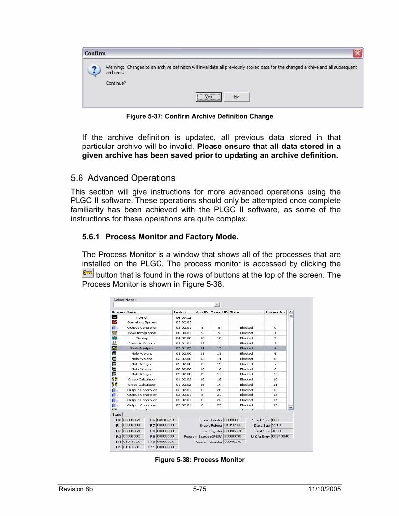
Revision 8b 5-75 11/10/2005
Figure 5-37: Confirm Archive Definition Change
If the archive definition is updated, all previous data stored in that particular archive will be invalid. Please ensure that all data stored in a given archive has been saved prior to updating an archive definition.
5.6 Advanced Operations This section will give instructions for more advanced operations using the PLGC II software. These operations should only be attempted once complete familiarity has been achieved with the PLGC II software, as some of the instructions for these operations are quite complex.
5.6.1 Process Monitor and Factory Mode.
The Process Monitor is a window that shows all of the processes that are installed on the PLGC. The process monitor is accessed by clicking the
button that is found in the rows of buttons at the top of the screen. The Process Monitor is shown in Figure 5-38.
Figure 5-38: Process Monitor

Section 5 Part Number MA2182
5-76
Most of the information present in the process monitor is valuable only for debugging purposes. However, it is useful to see a) which processes are running, and b) what the revision numbers of all the processes are. The column marked ‘State’ shows the current state of a process. The possible states are as follows:
• Blocked/Running – the process is running normally. • Terminated – the process has been ‘killed’. • Pending – the process is a newly installed process that needs to be
started. Right-clicking on a process that is marked ‘Blocked’ or ‘Running’ will bring up a menu with only one option – ‘Kill Current Process’. Selecting this option will cause the process to be killed or ‘terminated’, and the State of the process in the process monitor will be updated to reflect this fact. The only reason to terminate a process is if the process is suspected to be malfunctioning in some way. For example, if the LCD display on the front of the PLGC is observed to freeze up, terminating and restarting the Display process may un-freeze the display. If a ‘Terminated’ process is right-clicked, another menu will be brought up. This menu will have two options – ‘Remove Current Process’ or ‘Restart Current Process’. Do NOT select the Remove option, but instead restart the process. IMPORTANT: Terminating and/or removing processes will cause the PLGC to stop working correctly. Only terminate a process if it seems to be malfunctioning, and immediately restart it. Factory mode is the mode in the PLGC software that allows the user to make changes to the firmware on the PLGC. To enter factory mode, click on the ‘Tools’ menu at the top of the screen, and select ‘Factory’ mode. A password is required to enter factory mode – by default this is ‘fact’. Once in factory mode, the user can make changes to the firmware that allows the PLGC to operate. To add or replace processes, click the Update Firmware ( ) button at the top of the screen – this will bring up a pop-up window such as the one shown in Figure 5-39.
Figure 5-39: Update Firmware Window

Revision 8b 5-77 11/10/2005
Compare the Revision number of all the processes in the ‘Update Firmware’ window with the revision number of all the processes in the Process monitor. If there are any processes in the Process Monitor that have lower numbers than those in the Update Firmware window, these processes will need to be updated. Select the process to update in the Update Firmware window by left-clicking on it, and select the ‘Replace Existing Process’ option in the Update Option box. Then press the ‘Update Firmware’ button. A window asking which process to replace will appear, as shown in Figure 5-40.
Figure 5-40: Replace Existing Process Window
Ensure that the name of the process being replaced is the same as the name of the process being written. The new firmware will then be written to the analyzer. The updated process then needs to be started, so return to the Process Monitor. Find the process with the ‘Pending’ state, right-click on this process, and select ‘Start Current Process’. To add a new process, select the new Firmware to be added to the PLGC and choose the ‘Add New Process’ option in the Update Firmware window. The new process then needs to be started in the Process Monitor, as before. Before a new process can be seen and configured in the Devices tree on the left side of the screen, the user must log off and then log back in to the analyzer. Typically, the only processes that may need to be added to a PLGC once it has been configured at the factory may be more Mole Weight Calculators or Cross Calculators, for things such as Wobbe Index or Real BTU calculations. 5.6.2 Calculating Compressibility and Real BTU with the PLGC II
Real BTU is a measure of the real BTU content of natural gas. The BTU content values in the component table are based on the assumption that the gas in the pipeline behaves as an ideal gas. However, as the behaviour of all gases varies from the behaviour of ideal gases to some degree, the actual BTU content of the gas in a gas stream is slightly
Section 5 Part Number MA2182
5-78
different than the calculated ideal BTU value. The variance between the volume of an ideal gas and that of a real gas at a given temperature and pressure is known as the compressibility factor. The following instructions will let the user set up the PLGC to calculate both Compressibility Factor and Real BTU. These instructions assume that the Components Table contains only columns for the Heating Value and Specific Gravity.
1. Go to the Components Table (Section 5.5.2) and add 3 new columns. Call one column ‘Summation Factor’, the second ‘Base Pressure’, and the third ‘Calculation Factor’. The Summation Factors for all components are available in Table 10-1 in Appendix C. Enter the number 1 into all cells in the ‘Calculation Factor’ column, and enter the desired base pressure (14.696psia or 14.73psia) into all cells in the Base Pressure column. Ensure that the ideal BTU values for all components are correct for the chosen base pressure. Write the new Components Table into the analyzer.
2. Get the software into 'Factory' mode - do this by clicking on the 'Tools' menu and selecting 'Factory'. The password is 'fact'.
3. Select the 'Update Firmware' button - this is the button directly to the right of the button that has a key icon on it, and the icon on this button is a lightning bolt above a computer chip.
4. Choose the 'Add new process' update option, and select 'Cross Calculator' as the process to add. Press the 'Update Firmware' button.
5. Once the software update has completed, press the 'Process Monitor' button (the one with the key icon on it).
6. Scroll down to the newly added 'Cross Calculator' - it will have its state listed as 'Pending'. Right click on that process, and select 'Start Current Process'.
7. Repeat steps 3-6 for two more 'Cross Calculator' and 3 'Mole Weight Calculator'.
8. Disconnect from the analyzer, and reconnect. Enter Update Mode – Password is 2222.
9. Go to the 'Setup' portion of the directory tree on the left, and expand it. Go down to 'Mole Weight Calculators', and double click on the first process marked 'Unknown Process Name'. Give this the name 'Summation', select Thread Id: 12 for the Analysis Thread ID (or whatever it is on your analyzer - there should only be one choice in the pull-down menu) and Summation Factor for the Component Table Column. Ensure the 'Use Normalized Values' box is checked. Write this update to the analyzer.
10. Go to the second 'Unknown Process Name' mole weight calculator. Name this 'Base Pressure'. Again, assign the Analysis Thread ID, and select Base Pressure from the Component Table Column. Again, ensure the 'Use Normalized Values' box is checked. Write this update to the analyzer.
Revision 8b 5-79 11/10/2005
11. Go to the third 'Unknown Process Name' mole weight Calculator. Call this 'Calculation Factor'. Assign the Analysis Thread ID, select Calculation Factor for the Component Table Column, and again ensure that the Normalize box is checked. Write this update to the analyzer.
12. Select the 'Database' tab on the bottom of the directory tree. Select the 'Global Data Points' node, and under this node, select 'Additional GDPs'. Right click and select 'Create new Global Data Point' on the pull down menu. Give this GDP the name 'STR 1 Summation', and click OK.
13. Repeat step 12 5 more times, giving the GDPs the following names – STR 1 Z Calculation, STR 1 Calculation Factor, STR 1 Base Pressure, STR 1 Compressibility, and STR 1 Real BTU. Press the Write To Unit button to upload the changes to the database to the unit.
14. Repeat steps 12 and 13 two more times, replacing STR 1 with REF and CAL as the prefix for each GDP.
15. Repeat Steps 12 and 13 for any additional streams on the analyzer – replacing the STR 1 prefix with STR 2, STR 3, etc.
16. Return to the 'Devices' tab, and select 'Cross Calculators' under the Setup-Support Apps nodes - there should be 2 'Unknown Process Name' listed.
17. Select the first Cross Calculator. Give it the name 'Z Factor Calculation'. At the top right of the screen will be a boxed in set of pull down menus with the title 'Calculation'. From the first pull down menu, select Summation. Ensure the 'Normalized' box is checked. Press the button beside the second pull down menu until a multiplication sign is seen. From the second pull down menu, select Summation. Ensure it's normalized. Push the button beside the 3rd pull down menu until it shows a multiplication sign, and select 'Base Pressure' from the 3rd pull down menu. Check the Normalized box. Make sure the 4th pull down menu says 'Disabled'. Write these changes to the unit.
18. Select the second cross calculator. Give it the name 'Real BTU'. In the Calculation box, select 'Cross-Calculator (Thread ID XX)' in the first pull down menu. To determine the thread ID of the Z-Factor Calculation cross calculator, right-click on the Z Factor Cross Calculator in the Devices tree, and choose ‘Details’ from the pop-up menu. An information window such as the one shown in Figure 5-41 will appear. The Thread ID is seen as the fourth entry under the heading ‘Information from Unit’.
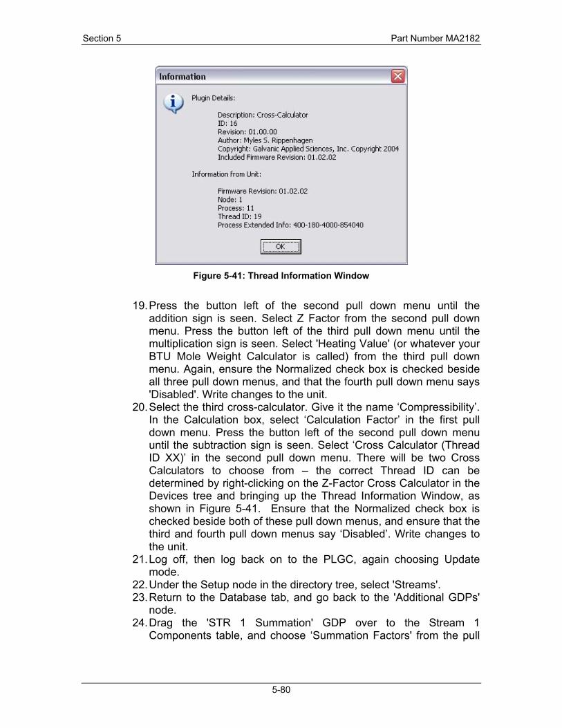
Section 5 Part Number MA2182
5-80
Figure 5-41: Thread Information Window
19. Press the button left of the second pull down menu until the
addition sign is seen. Select Z Factor from the second pull down menu. Press the button left of the third pull down menu until the multiplication sign is seen. Select 'Heating Value' (or whatever your BTU Mole Weight Calculator is called) from the third pull down menu. Again, ensure the Normalized check box is checked beside all three pull down menus, and that the fourth pull down menu says 'Disabled'. Write changes to the unit.
20. Select the third cross-calculator. Give it the name ‘Compressibility’. In the Calculation box, select ‘Calculation Factor’ in the first pull down menu. Press the button left of the second pull down menu until the subtraction sign is seen. Select ‘Cross Calculator (Thread ID XX)’ in the second pull down menu. There will be two Cross Calculators to choose from – the correct Thread ID can be determined by right-clicking on the Z-Factor Cross Calculator in the Devices tree and bringing up the Thread Information Window, as shown in Figure 5-41. Ensure that the Normalized check box is checked beside both of these pull down menus, and ensure that the third and fourth pull down menus say ‘Disabled’. Write changes to the unit.
21. Log off, then log back on to the PLGC, again choosing Update mode.
22. Under the Setup node in the directory tree, select 'Streams'. 23. Return to the Database tab, and go back to the 'Additional GDPs'
node. 24. Drag the 'STR 1 Summation' GDP over to the Stream 1
Components table, and choose ‘Summation Factors' from the pull
Revision 8b 5-81 11/10/2005
down menu in the 'Component Table Column' column of the table. Check the 'Normalized' check box.
25. Repeat Step 23 for the STR 1 Calculation Factor, STR 1 Z-factor Calculation, STR 1 Base Pressure, STR 1 Compressibility, and STR 1 Real BTU GDPs, ensuring that these are all normalized. Write changes to the unit.
26. Repeat Steps 23 and 24 for the Reference (REF), Calibration (CAL) and any additional sample streams, such as Stream 2 (STR 2), Stream 3 (STR 3), etc.
27. To output Real BTU to an analog output, under the Setup-Support Apps-Output Controllers node, select the analog output that is currently outputting the ideal heating value. Drag the desired stream’s ‘Real BTU' GDP to the 'Send this Value...' box, and write changes to the unit. The analog output will now be outputting real BTU rather than ideal BTU.
28. To output Real BTU to the archive, go to the Setup-Archive Setup node in the directory tree. Press the 'Add Archive' button, and call the archive 'Real BTU'. Drag any or all stream’s 'Real BTU' GDP over to the box, and select the checkbox marked 'Absolute Change Trigger'. In the box to the right, marked 'Absolute Change Amount', type in 0.0001. Near the bottom of the screen will be a box marked 'Maximum Records for this Archive'. Type in however many readings of Real BTU you want to store on the analyzer. In the pull down menu below the word 'Frequency', choose 'None'. Write Changes to the analyzer.
29. To output Compressibility to an analog output or archive, follow step 27 or 28 for the Compressibility GDP.
5.6.3 Calculation of Wobbe Index with PLGC
The Wobbe Index provides a method of comparing gas mixtures of varying composition, and it is a value indicating interchangeability of various fuel-gas mixtures. If two different gases have an identical Wobbe Index at a given pressure, they will produce an equal amount of heat and combustion products and will require the same amount of combustion air. To calculate Wobbe Index using the PLGC, follow these instructions. 1. Add one new Cross Calculator to the PLGC, and in the process
monitor, start this process. 2. Log off the unit, then log back on in Update Mode and go to the new
Cross Calculator. Call it Wobbe Index. In the first pull down menu in the ‘Calculation’ box, select the Cross Calculator that corresponds to the Real BTU calculation. Determine the Thread ID for the Real BTU Cross Calculator as before, by right clicking on the Real BTU Cross Calculator and selecting ‘Details’ from the pop-up menu. Ensure that the normalized checkbox is checked.

Section 5 Part Number MA2182
5-82
3. Press the button to the left of the second pull-down menu until an icon indicating the operation ‘divided by the square root of’ is seen. In the pull-down menu, choose Specific Gravity. Again, make sure that the normalized checkbox is checked. Write changes to the unit.
4. In the database, add GDPs for Wobbe Index in all streams – i.e. STR 1 Wobbe Index, STR 2 Wobbe Index… CAL Wobbe Index, REF Wobbe Index. Write the database changes to the unit.
5. Drag the Wobbe Index GDPs into their respective streams, and choose ‘Wobbe Index’ in the ‘Component Table Column’ column of the Components section of the streams window. Ensure that this is normalized in all streams. Write changes to the unit.
6. Create an archive or archives for Wobbe Index as per Step 28 of section 5.6.2. Output Wobbe index to the Analog Outputs as per Step 27 of section 5.6.2.
.
Revision 8b 6-83 11/10/2005
Section 6
6 Maintenance This section describes simple maintenance procedures that may be carried out in the field. If difficulty is encountered performing any of the maintenance procedures outlined in this section, technical assistance may be obtained from:
Galvanic Applied Sciences, Inc, 7000 Fisher Road SE
Calgary, Alberta T2H 0W3 CANADA
Phone: (403) 252-8470 Fax: (403) 255-6287
E-mail: [email protected] WARNING – Explosion Hazard – Do not disconnect equipment unless power has been switched off or the area is known to be non-hazardous AVERTISSEMENT – Risque d’explosion – avant de deconnecter l’equipement, couper le courant ou s’assurrer que l’emplacement est designe non dangereux WARNING – Explosion Hazard – Substitution of components may impair suitability for Class I, Division 2 AVERTISSEMENT – Risque d’explosion – La substitution de composants peut render ce material inacceptable pour les emplacements de Classe I, Division 2
6.1 Weekly Checkup
Your PLGC II gas chromatograph will provide reliable service with very little attention. However, a weekly check-up will ensure that the analyzer is operating according to specifications. The Weekly Check-up Report (Section 6.9) should be filled in, dated and kept on file. These reports will give a record of the analyzer's performance and will be useful in planning gas bottle replacement schedules as well as in troubleshooting. Flows and pressures are also recorded and should be adjusted as specified in the Configuration Report. The column temperature and baseline reading should also be recorded. If any of the diagnostic parameters are incorrect
Section 6 Part Number MA2182
6-84
consult the Troubleshooting Guide in this manual or contact Galvanic Applied Sciences.
6.2 Gas Cylinder Replacement Ideally, the helium cylinder should be replaced before it runs out. If the helium supply runs out the analyzer may require a 24-hour start up time. Galvanic Applied Sciences recommends using a two cylinder manifold system. A large helium cylinder should last 3 - 6 months depending on the application.
6.3 Cleaning the PLGC II When cleaning the exterior of the PLGC II, caution should be taken not to submerse the unit in water. Do not clean with a hose or with excessive amounts of water. A cleaner that is safe for use on stainless steel may be used to gently clean the unit. Do not attempt to clean any of the electronic equipment within the PLGC II.
6.4 Chromatograph Valve The most common cause of failure of a chromatograph valve is particle contamination in the sample or actuation gas. It is imperative that the sample is clean and dry. Please contact Galvanic Applied Sciences if assistance is required in designing a sample system suitable for the chosen application. The chromatograph valve must be cleaned or replaced if it is found to leak. A leak in the injection valve will typically be characterized by any of the following symptoms: elevated baseline, poor analyzer repeatability, poor back flush peak shape, a shift in the retention time of the back flush peak, or a second peak immediately following any valve actuation. Galvanic Applied Sciences recommends keeping a spare valve on hand. If a valve fails it can easily be changed out according to the procedure below. The failed valve can then be cleaned or rebuilt and kept on hand as a spare for possible future valve replacement. Please contact Galvanic Applied Sciences Inc. if a leaky valve is suspected before attempting to replace a valve. A model of a Valco 10-port valve is shown in Figure 6-1.
6.4.1 Procedure for Changing a Valve Step 1 Turn the analyzer to the ‘Halt’ mode. Step 2 Turn off the sample gas flow to the analyzer. Step 3 Turn off the helium gas flow to the analyzer. Step 4 Undo all ten fittings that go into the ten ports of the
valve.

Revision 8b 6-85 11/10/2005
Figure 6-1: Valco 10-port Valve
Step 5 Remove the valve by loosening the screws that hold
down the valve-mounting bracket. Step 6 Replace the valve and the mounting screws. Step 7 Re-connect the ten fittings to the correct ports. Re-
attach the actuation line. See the analyzer flow diagram in Section 2.1 for assistance.
Step 8 Return the helium flow to the analyzer. At this point the analyzer should be allowed to stabilize for 24 hours and is then ready to resume analysis.
6.5 Flow Control Stable helium pressure is very important to maintain repeatable retention times of the components. A dual stage regulator is recommended. Set the pressure as recorded in the Configuration Report. UHP helium is required. If UHP helium is not readily available, HP helium can be used with a series of scrubbers. Please call for specific recommendations. Sample pressure is not as critical but should be maintained at a constant pressure between 10 and 100 psig.
Notes Remember which connections were made to which ports. Also undo the air actuation line. This procedure also applies to 6-port valves, if the analyzer is equipped with such valves.
Valve fittings (numbered 1 – 10)
Valve actuation line
Clamping screw
Mounting holes
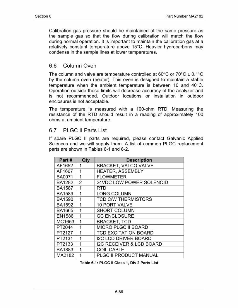
Section 6 Part Number MA2182
6-86
Calibration gas pressure should be maintained at the same pressure as the sample gas so that the flow during calibration will match the flow during normal operation. It is important to maintain the calibration gas at a relatively constant temperature above 15°C. Heavier hydrocarbons may condense in the sample lines at lower temperatures.
6.6 Column Oven The column and valve are temperature controlled at 60°C or 70°C ± 0.1°C by the column oven (heater). This oven is designed to maintain a stable temperature when the ambient temperature is between 10 and 40°C. Operation outside these limits will decrease accuracy of the analyzer and is not recommended. Outdoor locations or installation in outdoor enclosures is not acceptable. The temperature is measured with a 100-ohm RTD. Measuring the resistance of the RTD should result in a reading of approximately 100 ohms at ambient temperature.
6.7 PLGC II Parts List If spare PLGC II parts are required, please contact Galvanic Applied Sciences and we will supply them. A list of common PLGC replacement parts are shown in Tables 6-1 and 6-2.
Part # Qty Description
AF1652 1 BRACKET, VALCO VALVE AF1667 1 HEATER, ASSEMBLY BA0071 1 FLOWMETER BA1282 2 24VDC LOW POWER SOLENOID BA1587 1 RTD BA1589 1 LONG COLUMN BA1590 1 TCD C/W THERMISTORS BA1592 1 10 PORT VALVE BA1665 1 SHORT COLUMN EN1586 1 GC ENCLOSURE MC1653 1 BRACKET, TCD PT2044 1 MICRO PLGC II BOARD PT2127 1 TCD EXCITATION BOARD PT2131 1 I2C LCD DRIVER BOARD PT2133 1 I2C RECEIVER & LCD BOARD BA1883 1 COIL CABLE MA2182 1 PLGC II PRODUCT MANUAL
Table 6-1: PLGC II Class 1, Div 2 Parts List

Revision 8b 6-87 11/10/2005
Part # Qty Description AF1652 1 BRACKET, VALCO VALVE AF1667 1 HEATER, ASSEMBLY BA0071 1 FLOWMETER BA1282 2 24VDC LOW POWER SOLENOID BA1587 1 RTD BA1589 1 LONG COLUMN BA1590 1 TCD C/W THERMISTORS BA1592 1 10 PORT VALVE BA1665 1 SHORT COLUMN 1 GC XP ENCLOSURE MC1653 1 BRACKET, TCD PT2044 1 MICRO PLGC II BOARD PT2127 1 TCD EXCITATION BOARD PT2131 1 I2C LCD DRIVER BOARD PT2133 1 I2C RECEIVER & LCD BOARD BA1883 1 COIL CABLE MA2182 1 PLGC II PRODUCT MANUAL SA0618 1 I.S. Barrier
Table 6-2: PLGC II Class 1, Div 1 Parts List (XP Version)
6.8 Weekly Check-up Report
Do not adjust the helium pressure, as this will cause the retention times of the components to shift
Date: _______________ Checked By: _______________ Analyzer Serial Number: _______________ Helium Bottle Pressure: _______________
Sample Pressure As Found: __________ As Left: __________ Flow As Found: __________ As Left: __________ Diagnostics
Column Temperature: __________°C Baseline Reading __________mV


Revision 8b 7-89 11/10/2005
Section 7
7 Troubleshooting Problem Cause Corrective action
Two peaks observed in chromatogram immediately following a valve switch event.
The valve is leaking because it is dirty.
Disassemble the valve (see Appendix D), and clean the valve. Alternatively, a new clean valve can be installed, and the dirty valve can be sent back to Galvanic Applied Sciences Inc. for cleaning.
Large unidentifiable peak.
Possible contamination
Clean all tubing and solenoids with Isopropyl Alcohol and let dry completely. If problem persists and is negatively affecting results, contact Galvanic for assistance.
High Baseline TCD Excitation board baseline is set too high
Halt the analyzer, open the column oven, and adjust the screw marked ‘Baseline’ on the potentiometer on the electronics board inside the oven until the baseline reads lower. If the baseline continues to drift upwards after 24 hours, check the next troubleshooting tip.
High Baseline There is a leak Check all fittings inside and outside the oven. Tighten up any loose fittings. If the problem persists, disassemble the valve (as shown in Appendix D), and clean or replace the valve.
No flow when Cal. Is initiated.
Solenoid does not energize
Check that there is 24VDC at solenoid. Check that solenoid is wired to connector P5 terminals 1 and 2. If the solenoid still does not energize, replace solenoid.
Analyzer won’t turn on. No power Check power termination connectors. Check display power from motherboard connector P15(motherboard)-red, black going to P10(display) –red, black

Section 7 Part Number MA2182
7-90
Communication Error is displayed on your P.C.
Communication setup is incorrect.
Select the Communication icon in the PLGC II DIMAC software. Check that the correct Com Port has been selected. Check that the RS-232 cable is connected properly. Ensure that connection speed is correctly set (typically 115200 baud for RS-232 connection).
Erratic flow meter float Flow meter tube is contaminated.
Clean flow meter tube with isopropyl alcohol and dry with clean, dry instrument air.
Incorrect readings Peaks have shifted, integration parameters incorrect
Check that helium pressure is at 60 psig, and / or adjust retention times. Examine the chromatogram and determine if peaks have shifted or if integration parameters are not correct.
Analyzer reads 0.000 Analyzer is Halted or retention times have shifted.
Check Analysis Control to see if the analyzer is halted. Check the chromatogram to see if there is a problem with the integration of peaks.
Wrong Nitrogen/Methane readings
Poor Nitrogen/Methane separation
Check the chromatogram to see if the nitrogen/methane peak separation and integration parameters are correct. Check all fittings inside and outside the oven.
Baseline is unstable There is a leak Check all fittings. Ensure that helium pressure is stable at 60 psig.
Baseline is unstable. Temperature in the column oven is unstable.
Allow the temperature to stabilize inside the oven for 24 hours prior to carrying out another analysis.

Revision 8b 8-91 11/10/2005
Section 8
Appendix A: Theory of Gas Chromatography
What is Gas Chromatography? Gas chromatography is the separation of a gaseous mixture of compounds (solutes) into its individual components. By separating the sample, it is possible to identify the components present in the mixture, as well as the concentrations of those components.
Basic Parts and Terminology of a Gas Chromatograph Parts Carrier Gas – carries the sample gas through the column and to the detector. This is also called the ‘mobile phase’. Carrier Regulator – maintains a constant pressure of the carrier gas to ensure a constant carrier flow rate. Sample Valve – injects a measured amount of sample gas into the carrier. Column – a glass or metal tube that contains the stationary phase (to be described shortly). The sample gas passes through, and the components of the gas are separated within the column. Detector – senses the changes in property being measured as the individual components elute from the column. It identifies and, with a response factor, quantifies the components of the sample. Oven – The detector and column are maintained at a constant temperature by the oven. Constant temperature is essential to achieve proper separation of components.
Figure 8-1: Chromatograph Equipment
Terms Component – one specific species of the sample gas (i.e. methane, propane, etc.). Elution – the process of moving the separated sample components completely through the stationary phase. Mobile phase – an inert gas (helium) that carries the sample gas over the stationary phase through the column. It is also referred to as the carrier gas.

Appendix A Part Number MA2182
8-92
Flow of Mobile Phase
Interaction With Stationary Phase
Detector
LeastMost
InjectorTime = t1
Time = t2
Time = t3
Sample Gas Column
Stationary phase – an adsorptive material that is contained inside the column. The individual components of the sample gas will adsorb to the stationary phase by varying amounts, depending on molecular properties of those components.
How are the components separated? The components within a gas sample are separated in a gas chromatograph by distribution of the components between a ‘mobile phase’ and a ‘stationary phase’. A mobile phase is generally an inert gas such as helium, argon, or nitrogen. The mobile phase, which is also called the carrier gas, transports the sample gas through the column, where the stationary phase exists. The stationary phase is an adsorptive material that is contained inside the column. The individual components of the sample gas will adsorb (stick) to the stationary phase by different amounts. This is because the components to be separated have varying affinities (chemical attractions) for the stationary phase. Those components that have a higher affinity for the stationary phase will pass through the system more slowly than those components that have a lower affinity for the stationary phase. As a result of these differences in mobility, sample components will become separated from each other as they travel through the stationary phase in the column. The components will emerge from the column (elute) at different times. When the components reach the end of the column, they pass over the detector, where they are identified and their concentrations are determined. Figure 8-2 shows the separation process as the carrier gas moves the sample through the column.
Figure 8-2: Sample Gas Flow Through The Column
How are the Components Detected and Quantified? The purpose of a detector is to monitor the carrier gas as it emerges from the column and to generate a signal in response to variation in its composition due to eluted components. The type of detector used in the PLGC II is a Thermal Conductivity Detector (TCD).

Revision 8b 8-93 11/10/2005
The Thermal Conductivity Detector consists of four spiral wound filament wires supported inside cavities in a metal block. A constant DC current is applied to the filaments, which are arranged in a Wheatstone bridge configuration. When pure carrier and reference gas are flowing across the filaments, the heat loss, and thus filament temperature, is constant. This consistent filament temperature produces a constant filament resistance. The currents in the electronic bridge can be balanced to produce a zero signal level as a reference.
When a specific component enters the TCD with the carrier, the heat dissipated from the filaments on the measured side changes. The amount of change is dependent on the thermal conductivity of the gas, which is different for every component in the sample. This change in heat dissipation causes a change in electrical resistance, which leads to an imbalance in the electronic bridge. The resulting electrical signal is then used in conjunction with a Response Factor (see Appendix B) to measure the concentration of the component. Figure 8-3 shows an example of the TCD filament configuration.
Figure 8-3: TCD
The Chromatograph Output: The Chromatogram The signal output by the TCD is used to generate a chromatogram, which is a graph of detector response against time. The presence of a component will generate a spike in the TCD’s response, which appears as a ‘peak’ on the chromatogram. The components are identified by the microprocessor according to the length of time it takes them to elute from the column. The concentration of each component is calculated using a response factor determined during calibration with a certified standard. Figure 9-4 shows the different characteristics and definitions of a typical chromatogram, assuming two components called ‘A’ and ‘B’.
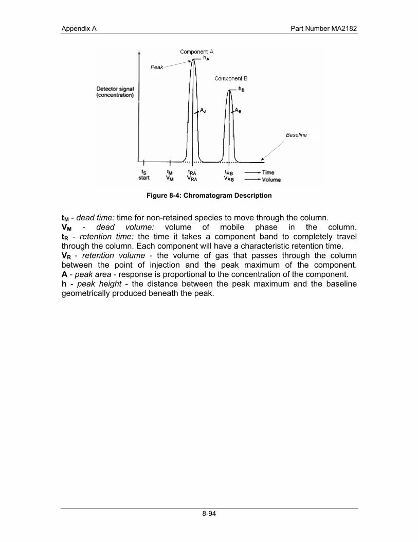
Appendix A Part Number MA2182
8-94
Figure 8-4: Chromatogram Description
tM - dead time: time for non-retained species to move through the column. VM - dead volume: volume of mobile phase in the column. tR - retention time: the time it takes a component band to completely travel through the column. Each component will have a characteristic retention time. VR - retention volume - the volume of gas that passes through the column between the point of injection and the peak maximum of the component. A - peak area - response is proportional to the concentration of the component. h - peak height - the distance between the peak maximum and the baseline geometrically produced beneath the peak.
Baseline
Peak

Revision 8b 9-95 11/10/2005
Section 9
Appendix B: Definitions and Formulas
Definition of Terms There are several terms used in this manual that the user should become familiar with. Baseline: A baseline is that portion of a chromatogram where
no detectable sample components emerge from the column. It appears as a flat line along the bottom of the chromatogram.
BTU: One “British Thermal Unit” is the quantity of heat required to raise one pound of water one degree Fahrenheit (° F) which is equivalent to 1.055056 x 10 -3 Mega-joules.
Chromatogram: A chromatogram is the permanent record of a single analysis run. It can be stored on a PC using the user interface software or recorded on a chart recorder. It displays the component peaks during an analysis cycle.
Component: Any one of several species that may appear in a sample. For example natural gas may contain several components such as Nitrogen, Methane, Carbon Dioxide, Ethane, propane, n-butane, iso-Butane, n-Pentane, iso-Pentane, and C6+.
Compressibility Factor: The ratio of the actual volume of a given mass of gas to the volume calculated from the ideal gas law under given temperature and pressure.
Dry BTU: The heating value of a standard cubic foot of gas saturated without water vapour.
Elution: The process of moving the separated sample components completely through the stationary phase.
Normalization: The process of multiplying the set of component concentrations by a constant factor to make their sum (or the sum of some related quantity) 1. Normalization is simply the re-expressing of component concentrations in terms of percents.
Peak: The measurement made by the PLGC II involves injecting a fixed sample volume into a carrier stream, which takes it to the detector. The detector sees the

Appendix B Part Number MA2182
9-96
sample that passes by it and produces an output that is approximately triangular in shape. This output can be viewed on the user interface software or a chart recorder and is referred to as a peak.
Peak Area: Peak area is the sum of the detector readings from the start to the end of the peak readings minus the baseline. Peak area is used to calculate response factors and concentrations.
Response Factor: The correction factor used to convert peak area into concentration.
The response factor is defined as: RF = Cal / Area
Where: RF = Response Factor
Area = area of the calibration peak Cal = concentration of the calibration sample
Retention Time: The time that elapses between the start of an analysis and the maximum height of a peak. Peak retention time is used to identify individual components in an analysis.
Saturated BTU: The heating value of a standard cubic foot of gas
saturated with water vapour. Specific Gravity: The ratio of the density of a substance to the density
of air at the same temperature. Standard Cubic Foot: The quantity or volume of gas occupying a cubic foot
of space at 60° F and 14.696 PSIA. Wobbe Index: The Wobbe Index is defined as the Gross Heating
Value divided by the square root of the Specific Gravity of the gas. It is an indicator of the interchangeability between different natural gas compositions.
Calibration Formulas and Analyzer Calculations A factory calibration is used to establish the response factors for each component and to determine the retention times of the species. The results of this calibration are available in the Configuration Report. Since the thermal conductivity of the various components is different, a calibration gas containing all of the components expected in the sample is required. Formulas for the response factor, as well as other calculations performed by the PLGC II, are as follows:

Revision 8b 9-97 11/10/2005
Response Factor While in the calibration mode the analyzer will measure several runs of the calibration standard. An average response factor will be calculated as shown in Definition of Terms. The response factor is used to calculate the concentration of the components in a run as shown below:
Concn = RFn * Arean
Where: Concn = concentration of components n RFn = response factor of components n Arean = area of peak produced by components n Compressibility Factor (Z) The compressibility factor is calculated as follows
Z = 1 – (Pb * ΣPn=1 [Concn * bn]
Where: Z = Compressibility factor Pb = Base pressure (psia) Concn = Normalized concentration of component n bn = ‘Summation factors’, as defined in GPA Standard 2172-96 Heating Values
Dry BTU
The energy content of the gas in BTU / cubic foot is calculated as follows:
Dry BTU / ft3 = ΣPn=1 [Concn * BTU / ft3n] / 100
Where: Dry BTU / ft3 = Dry BTU content per cubic foot of sample gas
Concn = Normalized concentration of component BTU/ft3n = BTU value of component n P = Number of components in the analysis Corrected Dry BTU Corrected Dry BTU / ft3 = (Dry BTU / ft3) / Z
Saturated BTU Sat BTU / ft3 = Dry BTU / ft3 x 0.9826 Where: Sat BTU /ft3 = Saturated BTU content per cubic foot of sample gas Dry BTU /ft3 = Dry BTU content per cubic foot of sample gas

Appendix B Part Number MA2182
9-98
Corrected Saturated BTU Corrected Sat BTU / ft3 = (Saturated BTU / ft3) / Z Specific Gravity (or Relative Density) The specific gravity of the gas is calculated as follows Dry Specific Gravity
Dry SG = (ΣPn=1 Concn x SGn) / 100
Where: Dry SG = Dry Specific Gravity of the sample gas
Concn = Normalized concentration of component n SGn = Specific Gravity value of component n P = Number of components in the analysis
Saturated Specific Gravity Sat SG = Dry SG*(1 – xw) + xw*0.62202 Where: Sat SG = Saturated specific gravity of the sample gas Dry SG = Dry Specific Gravity of the sample gas xw = molar fraction of water
Wobbe Index The Wobbe index is calculated as follows Dry Wobbe Index Dry Wobbe Index = (Corrected Dry BTU / ft3) / √(Dry SG) Saturated Wobbe Index Sat Wobbe Index = (Corrected Sat BTU / ft3) / √(Sat SG)
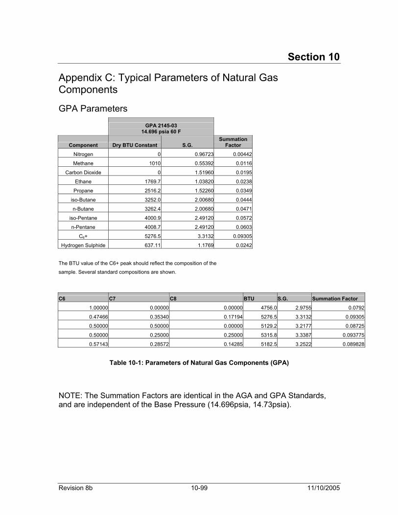
Revision 8b 10-99 11/10/2005
Section 10
Appendix C: Typical Parameters of Natural Gas Components
GPA Parameters
GPA 2145-03
14.696 psia 60 F
Component Dry BTU Constant S.G. Summation
Factor
Nitrogen 0 0.96723 0.00442
Methane 1010 0.55392 0.0116
Carbon Dioxide 0 1.51960 0.0195
Ethane 1769.7 1.03820 0.0238
Propane 2516.2 1.52260 0.0349
iso-Butane 3252.0 2.00680 0.0444
n-Butane 3262.4 2.00680 0.0471
iso-Pentane 4000.9 2.49120 0.0572
n-Pentane 4008.7 2.49120 0.0603
C6+ 5276.5 3.3132 0.09305
Hydrogen Sulphide 637.11 1.1769 0.0242
The BTU value of the C6+ peak should reflect the composition of the
sample. Several standard compositions are shown.
2.9755 3.4598 3.9441
4755.9 5502.5 6248.9
C6 C7 C8 BTU S.G. Summation Factor
1.00000 0.00000 0.00000 4756.0 2.9755 0.0792
0.47466 0.35340 0.17194 5276.5 3.3132 0.09305
0.50000 0.50000 0.00000 5129.2 3.2177 0.08725
0.50000 0.25000 0.25000 5315.8 3.3387 0.093775
0.57143 0.28572 0.14285 5182.5 3.2522 0.089828
Table 10-1: Parameters of Natural Gas Components (GPA)
NOTE: The Summation Factors are identical in the AGA and GPA Standards, and are independent of the Base Pressure (14.696psia, 14.73psia).

Appendix C Part Number MA2182
10-100
AGA Parameters
AGA 2145-00
14.696 psia 60 F
Component Dry BTU Constant S.G.
Argon 0.00 1.3793
Carbon Dioxide 0.00 1.5196
Ethane 1769.70 1.0382Hydrogen Sulphide 637.13 1.1767
Helium 0.00 0.1382
Heptane 5502.60 3.4598
Hexane 4756.00 2.9755
Hydrogen 324.20 0.0696
Carbon Monoxide 320.50 0.9671
i-Butane 3251.90 2.0068
i-Pentane 4000.90 2.4912
Methane 1010.00 0.5539
n-Butane 3262.40 2.0068
neo-Pentane 3985.00 2.4912
Nitrogen 0.00 0.9672
n-Pentane 4008.70 2.4912
Octane 6248.80 3.9441
Nonane 6996.20 4.4284
Decane 7742.90 4.9127
Ethylene 1600.40 0.9686
Propylene 2333.70 1.4529
Propane 2516.20 1.5225
Table 10-2: Parameters of Natural Gas Components (AGA)
AGA 2145-00
14.73 psia 60 F
Component Dry BTU Constant S.G.
Argon 0.00 1.3825
Carbon Dioxide 0.00 1.5231
Ethane 1773.79 1.0406Hydrogen Sulphide 638.60 1.1794
Helium 0.00 0.1385
Heptane 5515.33 3.4678
Hexane 4767.00 2.9824
Hydrogen 324.95 0.0698
Carbon Monoxide 321.24 0.9693
i-Butane 3259.42 2.0114
i-Pentane 4010.16 2.4970
Methane 1012.34 0.5552
n-Butane 3269.95 2.0114
neo-Pentane 3994.22 2.4970
Nitrogen 0.00 0.9695
n-Pentane 4017.97 2.4970
Octane 6263.26 3.9532
Nonane 7012.39 4.4386
Decane 7760.81 4.9241
Ethylene 1604.10 0.9708
Propylene 2339.10 1.4563
Propane 2522.02 1.5260

Revision 8b 11-101 11/10/2005
Section 11
Appendix D: Valco 6 and 10 Port Valve Technical Information
Valve Operation Instructions

Appendix D Part Number MA2182
11-102

Revision 8b 11-103 11/10/2005
Valve Maintenance Instructions

Appendix D Part Number MA2182
11-104
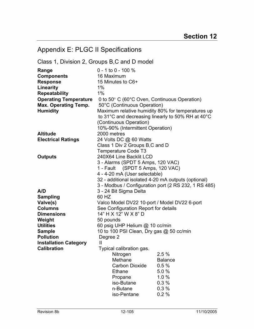
Revision 8b 12-105 11/10/2005
Section 12
Appendix E: PLGC II Specifications
Class 1, Division 2, Groups B,C and D model Range 0 - 1 to 0 - 100 % Components 16 Maximum Response 15 Minutes to C6+ Linearity 1% Repeatability 1% Operating Temperature 0 to 50° C (60°C Oven, Continuous Operation) Max. Operating Temp. 50°C (Continuous Operation) Humidity Maximum relative humidity 80% for temperatures up to 31°C and decreasing linearly to 50% RH at 40°C
(Continuous Operation) 10%-90% (Intermittent Operation)
Altitude 2000 metres Electrical Ratings 24 Volts DC @ 60 Watts
Class 1 Div 2 Groups B,C and D Temperature Code T3
Outputs 240X64 Line Backlit LCD 3 - Alarms (SPDT 5 Amps, 120 VAC)
1 - Fault (SPDT 5 Amps, 120 VAC) 4 - 4-20 mA (User selectable) 32 - additional isolated 4-20 mA outputs (optional)
3 - Modbus / Configuration port (2 RS 232, 1 RS 485) A/D 3 - 24 Bit Sigma Delta Sampling 60 HZ Valve(s) Valco Model DV22 10-port / Model DV22 6-port Columns See Configuration Report for details Dimensions 14” H X 12” W X 8” D Weight 50 pounds Utilities 60 psig UHP Helium @ 10 cc/min Sample 10 to 100 PSI Clean, Dry gas @ 50 cc/min Pollution Degree 2 Installation Category II Calibration Typical calibration gas.
Nitrogen 2.5 % Methane Balance Carbon Dioxide 0.5 % Ethane 5.0 % Propane 1.0 % iso-Butane 0.3 % n-Butane 0.3 % iso-Pentane 0.2 %

Appendix E Part Number MA2182
12-106
n-Pentane 0.2 % n-Hexane 0.1 %
Class 1, Division 1, Groups ,C and D model (Explosion Proof) Range 0 - 1 to 0 - 100 % Components 16 Maximum Response 15 Minutes to C6+ Linearity 1% Repeatability 1% Operating Temperature 0 to 50°C (Continuous Operation) Max. Operating Temp. 50°C (Continuous Operation) Humidity Maximum relative humidity 80% for temperatures up to 31°C and decreasing linearly to 50% RH at 40°C
(Continuous Operation) 10%-90% (Intermittent Operation)
Altitude 2000 metres maximum Electrical 110/220 VAC, 5 amps
Class 1 Div 1 Groups C and D Temperature Code T3
Outputs 240/64 Line Backlit LCD 3 - Alarms (SPDT 5 Amps, 120 VAC) 1 - Fault (SPDT 5 Amps, 120 VAC)
4 - 4-20 mA 32 - additional isolated 4-20 mA outputs (optional)
3 - ModBus / Configuration port (2 RS 232, 1 RS 485) A/D 3 - 24 Bit Sigma Delta Sampling 60 HZ Valve(s) Valco Model DV22 10-port / Model DV22 6-port Columns See Configuration Report for details Dimensions 30” H X 16” W X 9” D Weight 70 pounds Utilities 60 psig UHP Helium @ 10 cc/min Sample 10 to 100 PSI Clean, Dry gas @ 50 cc/min Pollution Degree 2 Installation Category II Calibration Typical calibration gas.
Nitrogen 2.5 % Methane Balance Carbon Dioxide 0.5 % Ethane 5.0 % Propane 1.0 % iso-Butane 0.3 % n-Butane 0.3 % iso-Pentane 0.2 % n-Pentane 0.2 % n-Hexane 0.1%

Revision 8b 12-107 11/10/2005