Physically-Based Simulation of Ice Formation

byTheodore Won-Hyung Kim

A dissertation submitted to the faculty of the University of North Carolina at ChapelHill in partial fulfillment of the requirements for the degree of Doctor of Philosophy inthe Department of Computer Science.

Chapel Hill2006

Approved byAdvisor: Ming C. LinReader: Mark Foskey

Reader: Anselmo LastraReader: David Adalsteinsson

Reader: Dinesh Manocha

ii

iii

c© 2006

Theodore Won-Hyung Kim

ALL RIGHTS RESERVED

iv

v

ABSTRACTTHEODORE WON-HYUNG KIM: Physically-Based Simulation of Ice

Formation.(Under the direction of Ming C. Lin.)

The geometric and optical complexity of ice has been a constant source of wonder

and inspiration for scientists and artists. It is a defining seasonal characteristic, so

modeling it convincingly is a crucial component of any synthetic winter scene. Like

wind and fire, it is also considered elemental, so it has found considerable use as a

dramatic tool in visual effects. However, its complex appearance makes it difficult for

an artist to model by hand, so physically-based simulation methods are necessary.

In this dissertation, I present several methods for visually simulating ice formation.

A general description of ice formation has been known for over a hundred years and

is referred to as the Stefan Problem. There is no known general solution to the Ste-

fan Problem, but several numerical methods have successfully simulated many of its

features. I will focus on three such methods in this dissertation: phase field methods,

diffusion limited aggregation, and level set methods.

Many different variants of the Stefan problem exist, and each presents unique chal-

lenges. Phase field methods excel at simulating the Stefan problem with surface tension

anisotropy. Surface tension gives snowflakes their characteristic six arms, so phase field

methods provide a way of simulating medium scale detail such as frost and snowflakes.

However, phase field methods track the ice as an implicit surface, so it tends to smear

away small-scale detail. In order to restore this detail, I present a hybrid method that

combines phase fields with diffusion limited aggregation (DLA). DLA is a fractal growth

algorithm that simulates the quasi-steady state, zero surface tension Stefan problem,

and does not suffer from smearing problems. I demonstrate that combining these two

algorithms can produce visual features that neither method could capture alone.

Finally, I present a method of simulating icicle formation. Icicle formation corre-

sponds to the thin-film, quasi-steady state Stefan problem, and neither phase fields nor

vi

DLA are directly applicable. I instead use level set methods, an alternate implicit front

tracking strategy. I derive the necessary velocity equations for level set simulation, and

also propose an efficient method of simulating ripple formation across the surface of

the icicles.

vii

ACKNOWLEDGMENTS

First, I want to thank my advisor, Ming Lin. If not for her physically-based modeling

course, I would not have found the seed of an idea that was later expanded into this

dissertation, and if not for her subsequent patience and support, I would not have been

able to develop and expand these ideas into their current form. Without her, this

dissertation would simply not exist. I would also like to thank all of my committee

members, David Adalsteinsson, Mark Foskey, Anselmo Lastra, and Dinesh Manocha,

for their patience and understanding, especially since this dissertation took a bit longer

than I had originally predicted.

I would also like to thank my parents and brother for their constant support through-

out my entire graduate career. Maybe this year, for the first time in five years, I won’t

spend Thanksgiving and Christmas cloistered away, working on a paper.

Without my friends in Chapel Hill, Karl Gyllstrom, Andrew Leaver-Fay, and Younoki

Lee, I am sure that burnout would have brutally truncated my graduate career long

ago. A special thanks to Younoki for her endless supply of delicious imitation crab

salad. I also want to thank my undergraduate roommate, Jeremy Kubica. Perhaps

this memory is apocryphal, but first semester freshman year, you said you wanted to

work in robotics, and I said I wanted to do graphics. If you’re reading this, it means

we now have PhDs in these fields.

My summer internships at Rhythm and Hues Studios in Los Angeles taught me

what industrial-strength code and movie production pipelines looks like, for which I

have to thank Jubin Dave and zuzu Spadaccini. You gave me an invaluable professional

experience, and more importantly, your friendship.

Last but not least, I thank my fiancee Ivy Bigelow for her endless support, enthu-

siasm, and encouragement. You give this work meaning.

viii

ix

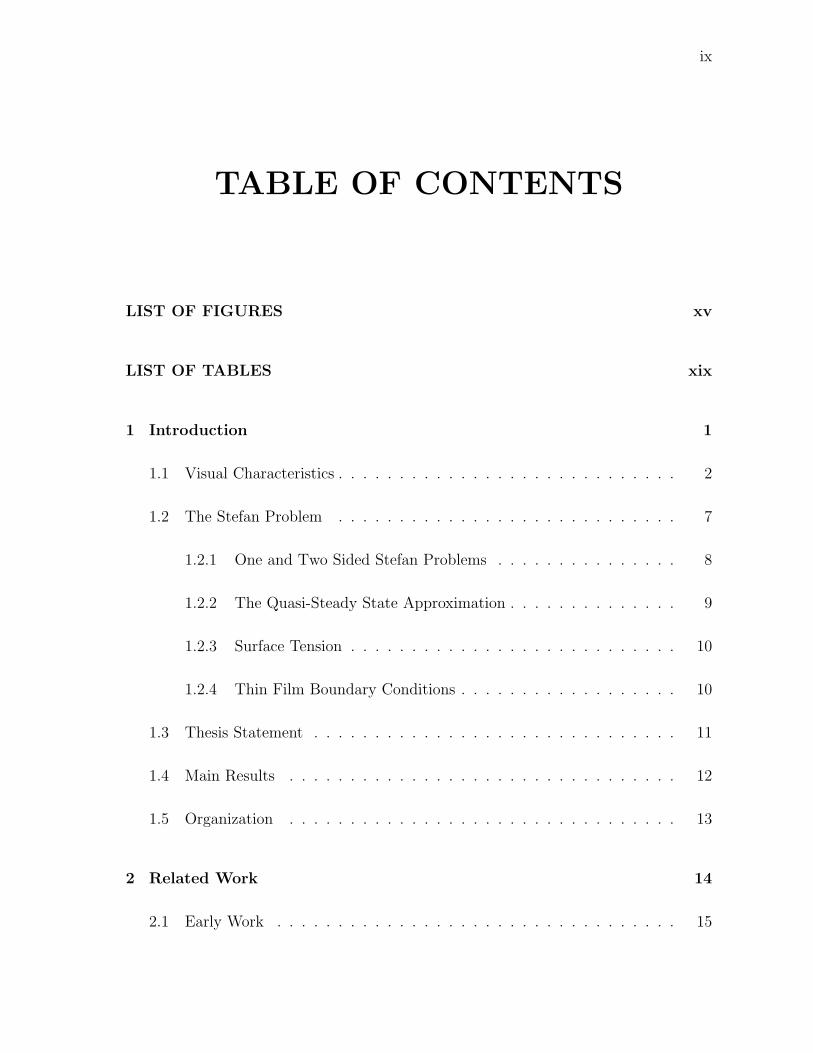
TABLE OF CONTENTS

LIST OF FIGURES xv

LIST OF TABLES xix

1 Introduction 1

1.1 Visual Characteristics . . . . . . . . . . . . . . . . . . . . . . . . . . . . 2

1.2 The Stefan Problem . . . . . . . . . . . . . . . . . . . . . . . . . . . . 7

1.2.1 One and Two Sided Stefan Problems . . . . . . . . . . . . . . . 8

1.2.2 The Quasi-Steady State Approximation . . . . . . . . . . . . . . 9

1.2.3 Surface Tension . . . . . . . . . . . . . . . . . . . . . . . . . . . 10

1.2.4 Thin Film Boundary Conditions . . . . . . . . . . . . . . . . . . 10

1.3 Thesis Statement . . . . . . . . . . . . . . . . . . . . . . . . . . . . . . 11

1.4 Main Results . . . . . . . . . . . . . . . . . . . . . . . . . . . . . . . . 12

1.5 Organization . . . . . . . . . . . . . . . . . . . . . . . . . . . . . . . . 13

2 Related Work 14

2.1 Early Work . . . . . . . . . . . . . . . . . . . . . . . . . . . . . . . . . 15

x

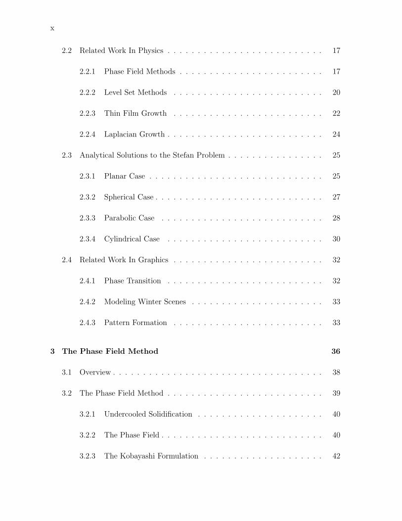
2.2 Related Work In Physics . . . . . . . . . . . . . . . . . . . . . . . . . . 17

2.2.1 Phase Field Methods . . . . . . . . . . . . . . . . . . . . . . . . 17

2.2.2 Level Set Methods . . . . . . . . . . . . . . . . . . . . . . . . . 20

2.2.3 Thin Film Growth . . . . . . . . . . . . . . . . . . . . . . . . . 22

2.2.4 Laplacian Growth . . . . . . . . . . . . . . . . . . . . . . . . . . 24

2.3 Analytical Solutions to the Stefan Problem . . . . . . . . . . . . . . . . 25

2.3.1 Planar Case . . . . . . . . . . . . . . . . . . . . . . . . . . . . . 25

2.3.2 Spherical Case . . . . . . . . . . . . . . . . . . . . . . . . . . . . 27

2.3.3 Parabolic Case . . . . . . . . . . . . . . . . . . . . . . . . . . . 28

2.3.4 Cylindrical Case . . . . . . . . . . . . . . . . . . . . . . . . . . 30

2.4 Related Work In Graphics . . . . . . . . . . . . . . . . . . . . . . . . . 32

2.4.1 Phase Transition . . . . . . . . . . . . . . . . . . . . . . . . . . 32

2.4.2 Modeling Winter Scenes . . . . . . . . . . . . . . . . . . . . . . 33

2.4.3 Pattern Formation . . . . . . . . . . . . . . . . . . . . . . . . . 33

3 The Phase Field Method 36

3.1 Overview . . . . . . . . . . . . . . . . . . . . . . . . . . . . . . . . . . . 38

3.2 The Phase Field Method . . . . . . . . . . . . . . . . . . . . . . . . . . 39

3.2.1 Undercooled Solidification . . . . . . . . . . . . . . . . . . . . . 40

3.2.2 The Phase Field . . . . . . . . . . . . . . . . . . . . . . . . . . . 40

3.2.3 The Kobayashi Formulation . . . . . . . . . . . . . . . . . . . . 42

xi

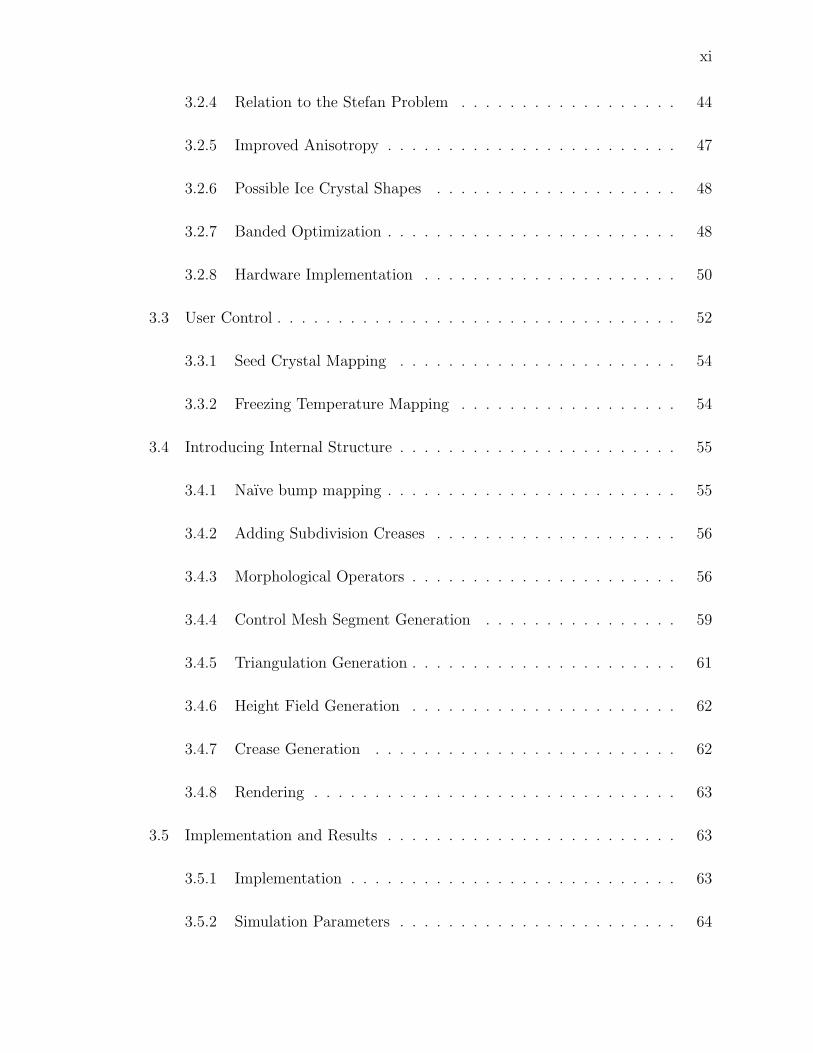
3.2.4 Relation to the Stefan Problem . . . . . . . . . . . . . . . . . . 44

3.2.5 Improved Anisotropy . . . . . . . . . . . . . . . . . . . . . . . . 47

3.2.6 Possible Ice Crystal Shapes . . . . . . . . . . . . . . . . . . . . 48

3.2.7 Banded Optimization . . . . . . . . . . . . . . . . . . . . . . . . 48

3.2.8 Hardware Implementation . . . . . . . . . . . . . . . . . . . . . 50

3.3 User Control . . . . . . . . . . . . . . . . . . . . . . . . . . . . . . . . . 52

3.3.1 Seed Crystal Mapping . . . . . . . . . . . . . . . . . . . . . . . 54

3.3.2 Freezing Temperature Mapping . . . . . . . . . . . . . . . . . . 54

3.4 Introducing Internal Structure . . . . . . . . . . . . . . . . . . . . . . . 55

3.4.1 Naıve bump mapping . . . . . . . . . . . . . . . . . . . . . . . . 55

3.4.2 Adding Subdivision Creases . . . . . . . . . . . . . . . . . . . . 56

3.4.3 Morphological Operators . . . . . . . . . . . . . . . . . . . . . . 56

3.4.4 Control Mesh Segment Generation . . . . . . . . . . . . . . . . 59

3.4.5 Triangulation Generation . . . . . . . . . . . . . . . . . . . . . . 61

3.4.6 Height Field Generation . . . . . . . . . . . . . . . . . . . . . . 62

3.4.7 Crease Generation . . . . . . . . . . . . . . . . . . . . . . . . . 62

3.4.8 Rendering . . . . . . . . . . . . . . . . . . . . . . . . . . . . . . 63

3.5 Implementation and Results . . . . . . . . . . . . . . . . . . . . . . . . 63

3.5.1 Implementation . . . . . . . . . . . . . . . . . . . . . . . . . . . 63

3.5.2 Simulation Parameters . . . . . . . . . . . . . . . . . . . . . . . 64

xii

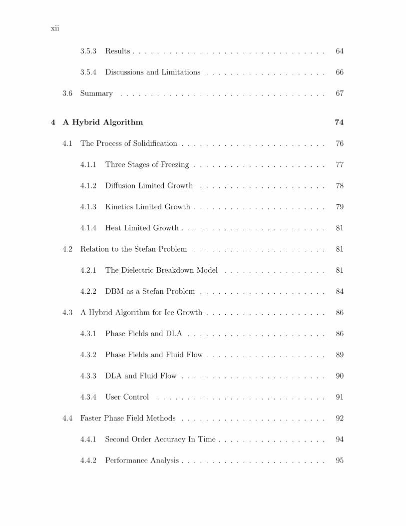
3.5.3 Results . . . . . . . . . . . . . . . . . . . . . . . . . . . . . . . . 64

3.5.4 Discussions and Limitations . . . . . . . . . . . . . . . . . . . . 66

3.6 Summary . . . . . . . . . . . . . . . . . . . . . . . . . . . . . . . . . . 67

4 A Hybrid Algorithm 74

4.1 The Process of Solidification . . . . . . . . . . . . . . . . . . . . . . . . 76

4.1.1 Three Stages of Freezing . . . . . . . . . . . . . . . . . . . . . . 77

4.1.2 Diffusion Limited Growth . . . . . . . . . . . . . . . . . . . . . 78

4.1.3 Kinetics Limited Growth . . . . . . . . . . . . . . . . . . . . . . 79

4.1.4 Heat Limited Growth . . . . . . . . . . . . . . . . . . . . . . . . 81

4.2 Relation to the Stefan Problem . . . . . . . . . . . . . . . . . . . . . . 81

4.2.1 The Dielectric Breakdown Model . . . . . . . . . . . . . . . . . 81

4.2.2 DBM as a Stefan Problem . . . . . . . . . . . . . . . . . . . . . 84

4.3 A Hybrid Algorithm for Ice Growth . . . . . . . . . . . . . . . . . . . . 86

4.3.1 Phase Fields and DLA . . . . . . . . . . . . . . . . . . . . . . . 86

4.3.2 Phase Fields and Fluid Flow . . . . . . . . . . . . . . . . . . . . 89

4.3.3 DLA and Fluid Flow . . . . . . . . . . . . . . . . . . . . . . . . 90

4.3.4 User Control . . . . . . . . . . . . . . . . . . . . . . . . . . . . 91

4.4 Faster Phase Field Methods . . . . . . . . . . . . . . . . . . . . . . . . 92

4.4.1 Second Order Accuracy In Time . . . . . . . . . . . . . . . . . . 94

4.4.2 Performance Analysis . . . . . . . . . . . . . . . . . . . . . . . . 95

xiii

4.5 Implementation and Results . . . . . . . . . . . . . . . . . . . . . . . . 96

4.6 Discussions and Limitations . . . . . . . . . . . . . . . . . . . . . . . . 98

4.7 Summary . . . . . . . . . . . . . . . . . . . . . . . . . . . . . . . . . . 100

5 Icicle Growth 107

5.1 The Stefan Problem . . . . . . . . . . . . . . . . . . . . . . . . . . . . 109

5.1.1 Background . . . . . . . . . . . . . . . . . . . . . . . . . . . . . 109

5.1.2 The Classic Stefan Problem . . . . . . . . . . . . . . . . . . . . 110

5.1.3 The Thin Film Stefan Problem . . . . . . . . . . . . . . . . . . 111

5.1.4 The Thin Film Ivantsov Parabola . . . . . . . . . . . . . . . . . 113

5.2 A Ripple Formation Model . . . . . . . . . . . . . . . . . . . . . . . . . 117

5.3 A Level Set Solver . . . . . . . . . . . . . . . . . . . . . . . . . . . . . 120

5.3.1 Background . . . . . . . . . . . . . . . . . . . . . . . . . . . . . 120

5.3.2 The Velocity Field . . . . . . . . . . . . . . . . . . . . . . . . . 121

5.3.3 Inserting the Icicle Tips . . . . . . . . . . . . . . . . . . . . . . 123

5.3.4 Tracking the Ripples . . . . . . . . . . . . . . . . . . . . . . . . 125

5.4 Rendering . . . . . . . . . . . . . . . . . . . . . . . . . . . . . . . . . . 125

5.5 Results and Validation . . . . . . . . . . . . . . . . . . . . . . . . . . . 128

5.6 Summary . . . . . . . . . . . . . . . . . . . . . . . . . . . . . . . . . . 130

6 Conclusion 136

xiv

6.1 Summary of Results . . . . . . . . . . . . . . . . . . . . . . . . . . . . 137

6.2 Limitations . . . . . . . . . . . . . . . . . . . . . . . . . . . . . . . . . 138

6.2.1 Phase Fields and DLA . . . . . . . . . . . . . . . . . . . . . . . 139

6.2.2 Icicle Simulation . . . . . . . . . . . . . . . . . . . . . . . . . . 140

6.2.3 Rendering Issues . . . . . . . . . . . . . . . . . . . . . . . . . . 141

6.3 Future Work . . . . . . . . . . . . . . . . . . . . . . . . . . . . . . . . . 142

A Cg Implementation of Phase Fields 145

Bibliography 151

xv

LIST OF FIGURES

1.1 Taxonomy of Snowflakes . . . . . . . . . . . . . . . . . . . . . . . . . . 3

1.2 Snowflake Photographs . . . . . . . . . . . . . . . . . . . . . . . . . . . 4

1.3 Combination of plate and dendritic growth . . . . . . . . . . . . . . . . 4

1.4 Photograph of frost . . . . . . . . . . . . . . . . . . . . . . . . . . . . . 5

1.5 Icicles On a Fountain . . . . . . . . . . . . . . . . . . . . . . . . . . . . 6

1.6 One-sided Stefan problem . . . . . . . . . . . . . . . . . . . . . . . . . 9

2.1 von Koch Snowflake . . . . . . . . . . . . . . . . . . . . . . . . . . . . . 16

3.1 Closeup of ice on a stained glass window . . . . . . . . . . . . . . . . . 38

3.2 Phase field system pipeline . . . . . . . . . . . . . . . . . . . . . . . . . 39

3.3 Cross-section of phase fields . . . . . . . . . . . . . . . . . . . . . . . . 41

3.4 Comparison of phase field snowflakes to real snowflakes . . . . . . . . . 45

3.5 Phase field controls . . . . . . . . . . . . . . . . . . . . . . . . . . . . . 53

3.6 Border extraction operation . . . . . . . . . . . . . . . . . . . . . . . . 57

3.7 Structuring Elements . . . . . . . . . . . . . . . . . . . . . . . . . . . . 58

3.8 Results of modified erosion operator . . . . . . . . . . . . . . . . . . . . 58

3.9 Skeletonization structuring elements . . . . . . . . . . . . . . . . . . . . 59

3.10 Results of skeleton and border operations . . . . . . . . . . . . . . . . . 60

3.11 Crease pixel types . . . . . . . . . . . . . . . . . . . . . . . . . . . . . . 60

xvi

3.12 Sharpening Results . . . . . . . . . . . . . . . . . . . . . . . . . . . . . 61

3.13 Lilypad ice growth . . . . . . . . . . . . . . . . . . . . . . . . . . . . . 65

3.14 Ice ring growth . . . . . . . . . . . . . . . . . . . . . . . . . . . . . . . 69

3.15 Ice growth on a window panel . . . . . . . . . . . . . . . . . . . . . . . 70

3.16 Ice growing on a red stained glass window . . . . . . . . . . . . . . . . 71

3.17 Ice growing on a stained glass window . . . . . . . . . . . . . . . . . . 72

3.18 Light refracting through a stained glass window . . . . . . . . . . . . . 73

4.1 A microscopic view of the three stages of freezing . . . . . . . . . . . . 76

4.2 Grid anisotropy in diffusion limited aggregation. . . . . . . . . . . . . . 79

4.3 Stencils and initial conditions for DBM . . . . . . . . . . . . . . . . . . 82

4.4 Comparison of DBM and DLA . . . . . . . . . . . . . . . . . . . . . . . 84

4.5 Finite difference stencils for a hexagonal grid . . . . . . . . . . . . . . . 88

4.6 A 4-armed dendrite growing in a flow . . . . . . . . . . . . . . . . . . . 91

4.7 Phase fields with and without diagonal terms . . . . . . . . . . . . . . 93

4.8 Frosty ice forming on a chilled glass . . . . . . . . . . . . . . . . . . . . 102

4.9 Ice Accumulated on a car . . . . . . . . . . . . . . . . . . . . . . . . . 103

4.10 Frost forming on a window . . . . . . . . . . . . . . . . . . . . . . . . . 104

4.11 Comparison to hybrid algorithm to DLA and phase fields . . . . . . . . 105

4.12 Validation of hybrid algorithm against a photograph . . . . . . . . . . . 106

4.13 Snowflake growths . . . . . . . . . . . . . . . . . . . . . . . . . . . . . 106

xvii

5.1 2D slice of parabolic coordinate system . . . . . . . . . . . . . . . . . . 115

5.2 Ray traced icicle star . . . . . . . . . . . . . . . . . . . . . . . . . . . . 126

5.3 BSSRDF icicle star . . . . . . . . . . . . . . . . . . . . . . . . . . . . . 127

5.4 Experimental validation of thin-film Ivantsov parabola . . . . . . . . . 130

5.5 Icicle star . . . . . . . . . . . . . . . . . . . . . . . . . . . . . . . . . . 132

5.6 Icicle star forming . . . . . . . . . . . . . . . . . . . . . . . . . . . . . . 133

5.7 A freezing fountain . . . . . . . . . . . . . . . . . . . . . . . . . . . . . 134

5.8 Ice forming on a roof . . . . . . . . . . . . . . . . . . . . . . . . . . . . 135

xviii

xix

LIST OF TABLES

2.1 Symbols for the Makkonen model . . . . . . . . . . . . . . . . . . . . . 23

3.1 Phase field constants . . . . . . . . . . . . . . . . . . . . . . . . . . . . 43

3.2 Banded vs. Unbanded Performance . . . . . . . . . . . . . . . . . . . . 50

3.3 CPU vs. GPU performance . . . . . . . . . . . . . . . . . . . . . . . . 52

4.1 Phase field performance over different resolutions . . . . . . . . . . . . 96

4.2 Timing results for simulation . . . . . . . . . . . . . . . . . . . . . . . . 97

5.1 Table of icicle symbols. . . . . . . . . . . . . . . . . . . . . . . . . . . . 117

5.2 Icicle Growth Data . . . . . . . . . . . . . . . . . . . . . . . . . . . . . 131

xx

Chapter 1

Introduction

Many years later, as he faced the firing squad, Colonel Aureliano Buendıa

was to remember that distant afternoon when his father took him to discover

ice.

– Gabriel Garcia Marquez, One Hundred Years of Solitude

Ice formations are one of the most memorable and visually arresting phenomena in

nature. On cold mornings, branching frost patterns can be found on sidewalks, window

panes, and car windshields. No winter scene would be complete without icicles dangling

from tree branches and rooftops. These formations are interesting because they exhibit

a high degree of geometric and optical complexity. As the old adage says: “No two

snowflakes are alike.” The same could pedantically be said about any collection of

objects, but the saying rings true for snowflakes because they span such a wide variety of

geometric forms. Because ice is translucent, this geometric complexity also translates to

optical complexity. Ice stands out in marked contrast to the smooth, diffuse reflections

of snow because it produces glittering, highly specular light interactions.

Scientific fascination with ice formation dates back to at least the birth of modern

science. Johannes Kepler first wrote of the six-fold symmetry of the snowflake almost

400 years ago (Kepler, 1611). Rene Descartes, a contemporary of Kepler, later wrote

about the wide variety of snowflakes he observed with the naked eye and pondered

their formation mechanism (Frank, 1974). Robert Hooke examined snowflakes using a

2

compound microscope and included sketches of what he saw in his book Micrographia

(Hooke, 1665). At the time, a more extensive quantitative analysis of ice formation

was not possible because thermodynamics was still poorly understood.

Like wind and fire, ice is viewed as elemental, so it has found considerable use as

a dramatic tool in visual effects. Its use predates the adoption of digital effects in the

film industry, and plays a pivotal role in such scenes as the formation of the Fortress

of Solitude in the 1978 film Superman, and the freezing death of Jack Torrance in

the 1980 film The Shining. More recently, digital freezing effects were used to great

dramatic effect in the 2004 film Harry Potter and the Prisoner of Azkaban. The ominous

appearance of frost was used to signify the arrival of the movie’s villains, the Dementors.

A film from the same year, The Day After Tomorrow, follows the flight of its characters

from a rapidly advancing ice age, and made extensive use of freezing effects. In this

case, ice was the villain. Numerous other recent movies have made prominent use of

digital freezing effects, such as Die Another Day, The Hulk, The Incredibles, The Lion

the Witch and the Wardrobe, Van Helsing, and X-Men 2.

1.1 Visual Characteristics

The goal of this dissertation is to faithfully simulate the interesting visual features of

ice, so the first step is to define which visual features give ice formations their enduring

appeal. Any list of such features is at best a set of conjectures, so the remainder of the

dissertation will be devoted to demonstrating that the features I have chosen do in fact

reproduce much of ice’s appeal. Once this feature list has been defined, I will devise

methods of efficiently simulating the mechanisms that give rise to these features.

In the case of snowflakes, a precise characterization of geometric structure can be

difficult, because part of their appeal is that they often take on novel and surprising

structures. Crystal growth is an active area of research, and extensive empirical ob-

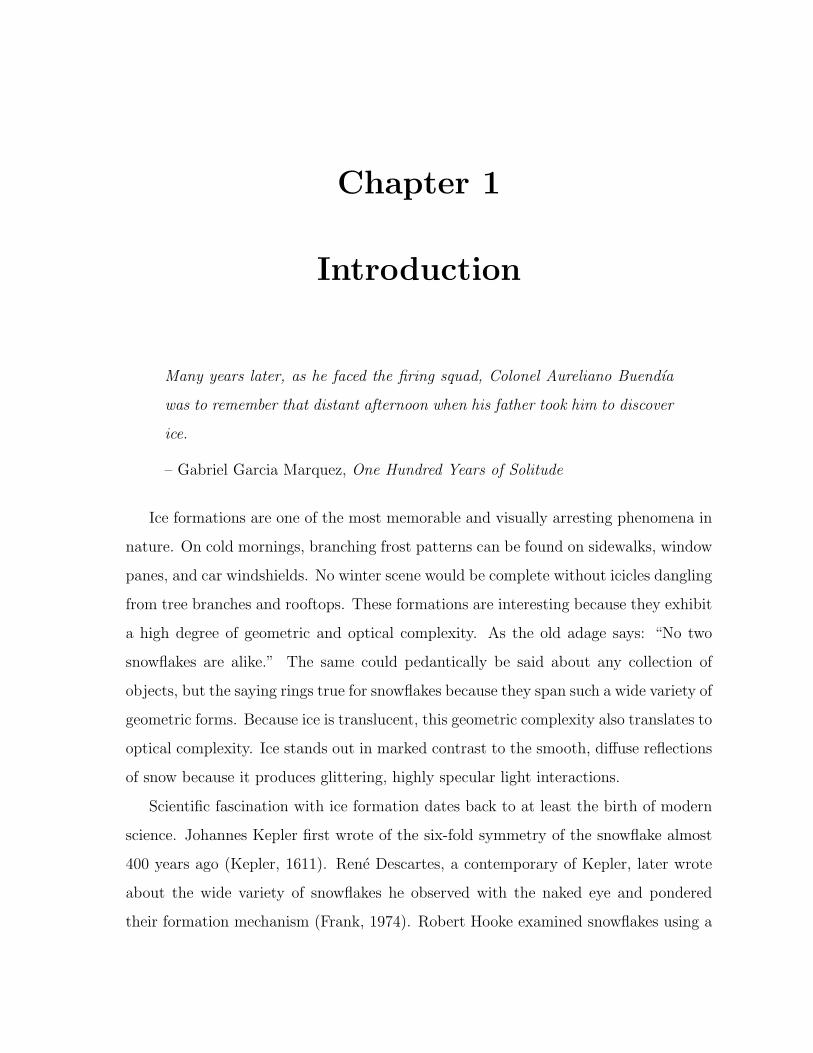
servation of snowflakes has yielded the taxonomy in Figure 1.1. However, Figure 1.1

provides a larger taxonomy than necessary for visual simulation. The hollow prism

3

Figure 1.1: Taxonomy of Snowflakes: Extensive empirical observation of snowflakeshave yielded a taxonomy of shapes. The widely varying geometry of snowflakes can beattributed to changing environmental conditions during formation. (From (Yokoyamaand Kuroda, 1990))

and solid column types, for example, refer to three dimensional snowflakes that can

be produced in laboratory settings, but are usually not observed in a typical winter

scene. Instead, most snowflakes can be viewed as existing on the continuum between

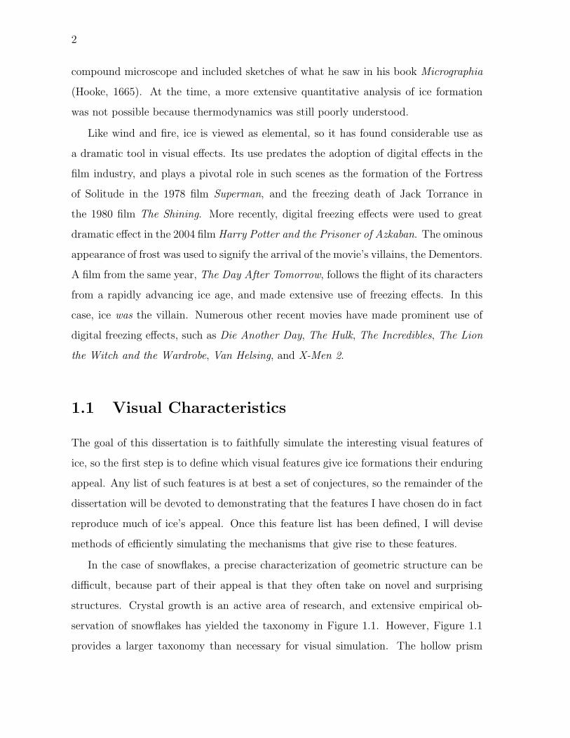
‘dendritic’ and ‘sectored plate’ growth. ‘Dendritic’ literally derives from ‘tree-like’ or

‘bush-like’, and refers to thin, spindly features, such as the snowflake on the far right of

Figure 1.2. ‘Sectored plate’ refers to the hexagonal growth pattern on the far left of Fig-

ure 1.2. Several examples of intermediate growth conditions in between can be seen in

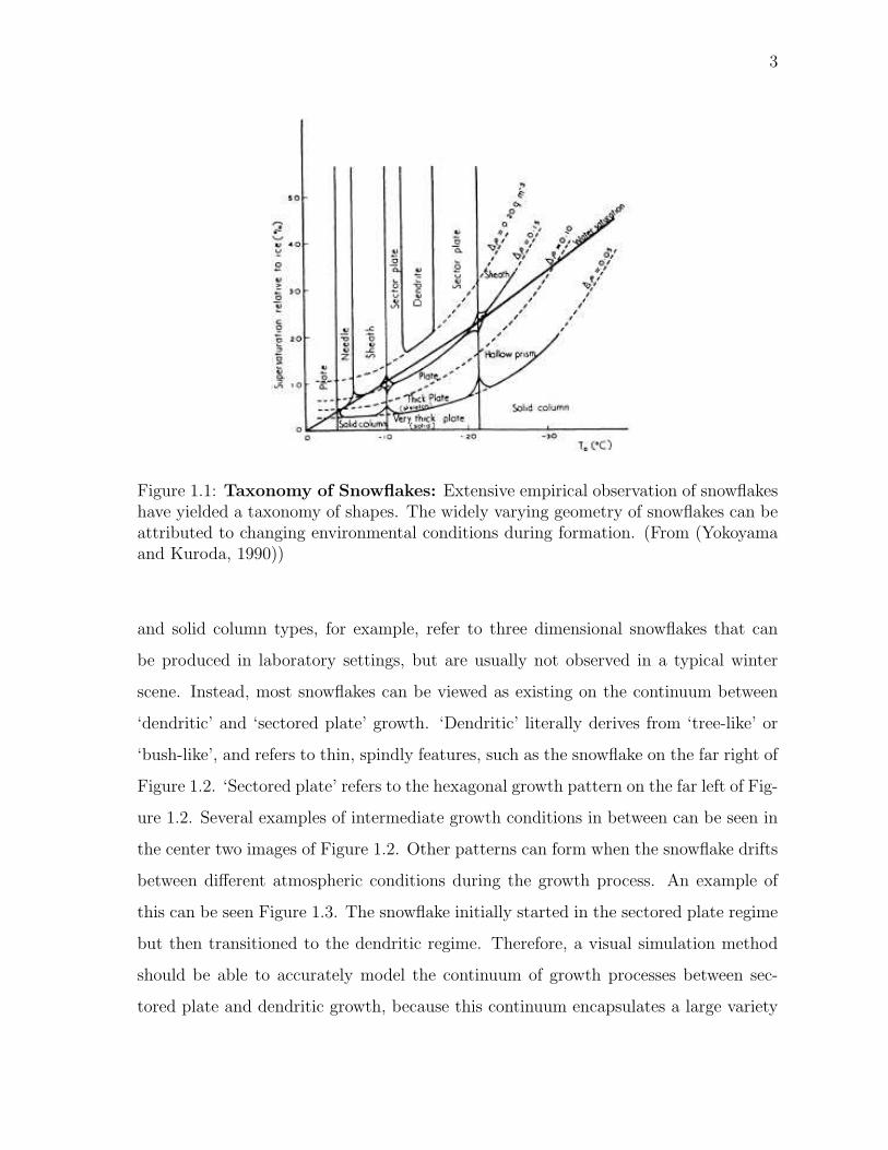
the center two images of Figure 1.2. Other patterns can form when the snowflake drifts

between different atmospheric conditions during the growth process. An example of

this can be seen Figure 1.3. The snowflake initially started in the sectored plate regime

but then transitioned to the dendritic regime. Therefore, a visual simulation method

should be able to accurately model the continuum of growth processes between sec-

tored plate and dendritic growth, because this continuum encapsulates a large variety

4

Figure 1.2: Snowflake Photographs: From left to right, the snowflake shapes transi-tion from sectored plate growth to dendritic growth. Photographs are from the Wilson“Snowflake” Bentley collection. (Bentley, 1902)

Figure 1.3: Combination of Plate and Dendritic Growth: This snowflake begangrowing in conditions that favored sectored plate growth, but at some point driftedinto atmospheric conditions amenable to dendritic growth. This photograph is fromthe Wilson “Snowflake” Bentley collection. (Bentley, 1902)

of crystal structures.

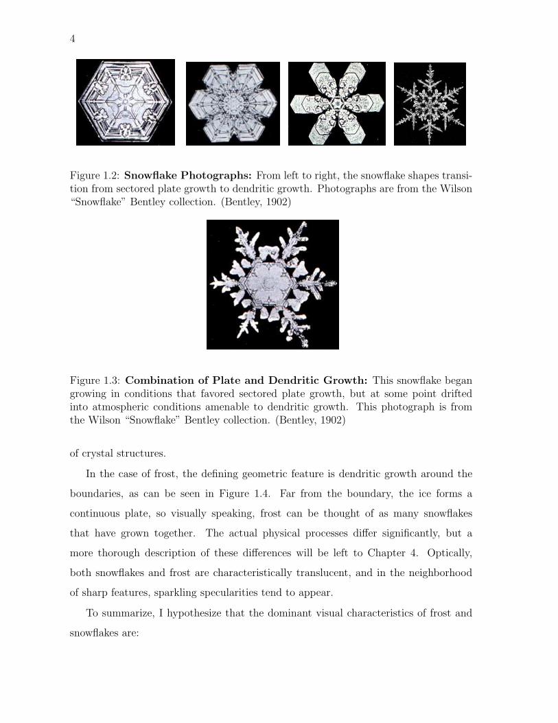
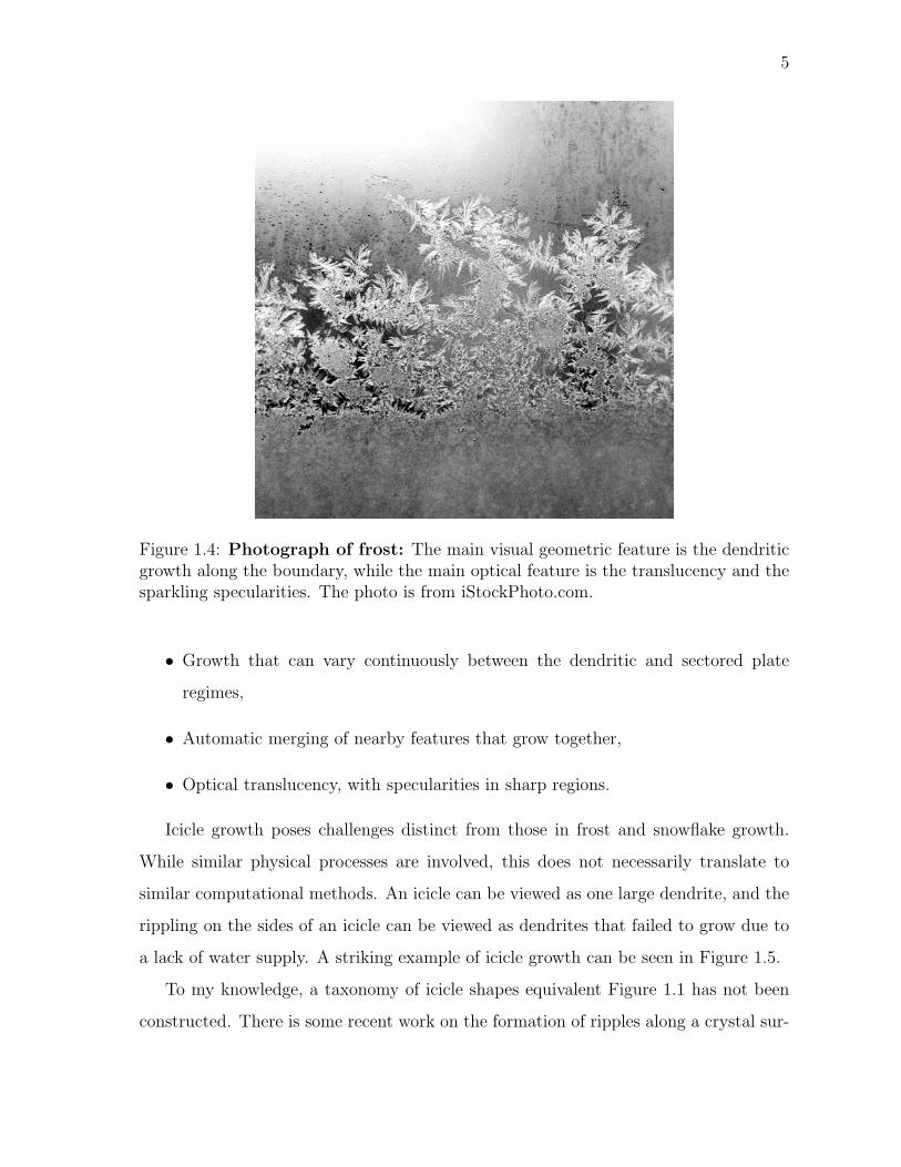
In the case of frost, the defining geometric feature is dendritic growth around the

boundaries, as can be seen in Figure 1.4. Far from the boundary, the ice forms a

continuous plate, so visually speaking, frost can be thought of as many snowflakes

that have grown together. The actual physical processes differ significantly, but a

more thorough description of these differences will be left to Chapter 4. Optically,

both snowflakes and frost are characteristically translucent, and in the neighborhood

of sharp features, sparkling specularities tend to appear.

To summarize, I hypothesize that the dominant visual characteristics of frost and

snowflakes are:

5

Figure 1.4: Photograph of frost: The main visual geometric feature is the dendriticgrowth along the boundary, while the main optical feature is the translucency and thesparkling specularities. The photo is from iStockPhoto.com.

• Growth that can vary continuously between the dendritic and sectored plate

regimes,

• Automatic merging of nearby features that grow together,

• Optical translucency, with specularities in sharp regions.

Icicle growth poses challenges distinct from those in frost and snowflake growth.

While similar physical processes are involved, this does not necessarily translate to

similar computational methods. An icicle can be viewed as one large dendrite, and the

rippling on the sides of an icicle can be viewed as dendrites that failed to grow due to

a lack of water supply. A striking example of icicle growth can be seen in Figure 1.5.

To my knowledge, a taxonomy of icicle shapes equivalent Figure 1.1 has not been

constructed. There is some recent work on the formation of ripples along a crystal sur-

6

Figure 1.5: Icicles On a Fountain: Photo is from BigFoto.com.

face (Ueno, 2003; Ueno, 2004), the author of these articles admits that the thermody-

namics of thin film flows still has many open questions, making analysis and taxonomy

construction difficult. However, the major visual features of icicles can be conjectured

from photos such as Figure 1.5. The first, most high-level observation is that icicles

are conical structures that are much longer than they are thick. Second, when two

icicles grow near to each other, their roots merge. Lastly, the small scale rippling on

the surface of icicles cause large scale optical effects, such as rippled specularities and

distorted refractions.

Explicitly, the dominant visual features of icicles are:

• Conical geometry that is much longer than it is wide,

• Automatic merging of nearby icicle roots,

• Optical effects caused by surface rippling.

7

1.2 The Stefan Problem

All of the previously listed visual characteristics can be understood in terms of the

Stefan problem. The Stefan problem was formulated in 1889 by Josef Stefan (Stefan,

1889), who is perhaps best known for the Stefan-Boltzmann law, which relates the

energy radiated by a blackbody emitter to its temperature. As a prominent scientific

mind at the time when the laws of thermodynamics were first becoming well understood,

Stefan was in a prime position to start addressing solidification problems.

Stefan posed his problem in the context of ocean ice forming in arctic regions,

but the problem has come to represent phase transition problems in general, and has

found applications in fields ranging from geology to metallurgy. The richly non-linear

behavior of the problem has also attracted considerable interest in mathematics (Hill,

1987; Meirmanov, 1992). An excellent historical overview of the problem is available

in (Wettlaufer, 2001). While the visual characteristics just listed can be captured in

the context of Stefan problems, they each require a different version of the problem,

which in turn requires different computational approaches. As the Stefan problem is

the theoretical thread that unifies all of these approaches, I will now provide a high

level description of the problem and describe the various versions and approximations

that will later be employed.

The Stefan problem is composed of two simple equations. Assume we have a heat

field T defined continuously over some computational domain, and an initial ice/water

interface Γ. The heat field evolves according to the heat equation

∂T

∂t= D∇2T, (1.1)

where t denotes time and D denotes a diffusion constant. The symbol ∇2 is the Lapla-

cian operator, which expands to ∂2

∂x2 + ∂2

∂y2 in 2D and ∂2

∂x2 + ∂2

∂y2 + ∂2

∂z2 in 3D. The ice/water

interface then evolves in the normal direction according to

∂Γ

∂t· n = D

∂T

∂n, (1.2)

8

where n denotes the normal direction. Fluid velocity and the coefficient of expansion

of ice are assumed to be negligible. Stefan stated the 1D version of this problem,

essentially approximating the ocean as a column of water. In 1D, the equations reduce

to:

dT

dt= D

d2T

dx2(1.3)

dΓ

dt= D

dT

dx, (1.4)

where x is the spatial coordinate. The location of the ice front Γ is then obtained by

integrating Eqns. 5.1 and 1.2. There are only a handful of known closed form solutions,

and these only apply to simple geometries. Stefan originally solved the planar case,

and subsequently the case of a sphere (Frank, 1949) and a parabola (Ivantsov, 1947)

were derived. These cases are often referred to eponymously as the “Frank sphere”

and “Ivantsov parabola” solutions. In the absence of a general analytical solution,

solutions are usually obtained numerically. Depending on the approximations used

and the boundary conditions assigned, various flavors of the Stefan problem can be

obtained. In this dissertation, I will deal with the following variants: one and two

sided, quasi-steady state, zero surface tension, and surface tension anisotropy.

1.2.1 One and Two Sided Stefan Problems

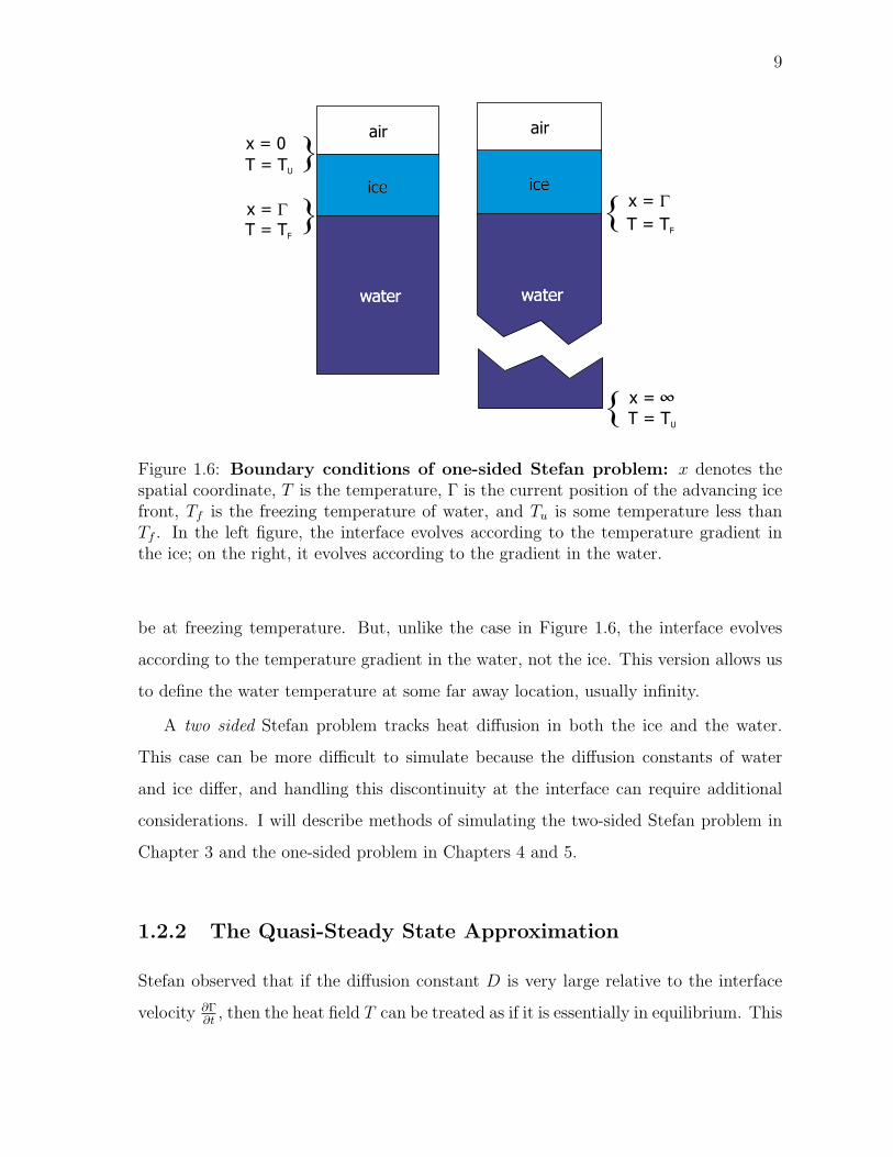
Stefan originally described the boundary conditions shown in the left half of Figure 1.6.

In this case, heat diffusion only occurs in the ice, and the air and water are assumed

to be at a constant temperature. Since the thermal conductivity of air and water is

smaller than that of ice, the heat loss to these media is assumed to be negligible. This is

known as a one sided Stefan problem, since it only takes into account heat diffusion on

one side of the ice/water interface. The complementary case is shown on the right side

of Figure 1.6, where heat diffusion is instead tracked in the water layer. In this case, we

assume that solidification is taking place, which means that the interface x = Γ must

9

Figure 1.6: Boundary conditions of one-sided Stefan problem: x denotes thespatial coordinate, T is the temperature, Γ is the current position of the advancing icefront, Tf is the freezing temperature of water, and Tu is some temperature less thanTf . In the left figure, the interface evolves according to the temperature gradient inthe ice; on the right, it evolves according to the gradient in the water.

be at freezing temperature. But, unlike the case in Figure 1.6, the interface evolves

according to the temperature gradient in the water, not the ice. This version allows us

to define the water temperature at some far away location, usually infinity.

A two sided Stefan problem tracks heat diffusion in both the ice and the water.

This case can be more difficult to simulate because the diffusion constants of water

and ice differ, and handling this discontinuity at the interface can require additional

considerations. I will describe methods of simulating the two-sided Stefan problem in

Chapter 3 and the one-sided problem in Chapters 4 and 5.

1.2.2 The Quasi-Steady State Approximation

Stefan observed that if the diffusion constant D is very large relative to the interface

velocity ∂Γ∂t

, then the heat field T can be treated as if it is essentially in equilibrium. This

10

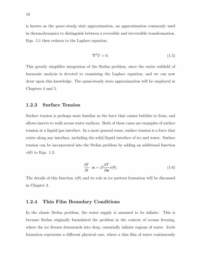
is known as the quasi-steady state approximation, an approximation commonly used

in thermodynamics to distinguish between a reversible and irreversible transformation.

Eqn. 5.1 then reduces to the Laplace equation:

∇2T = 0. (1.5)

This greatly simplifies integration of the Stefan problem, since the entire subfield of

harmonic analysis is devoted to examining the Laplace equation, and we can now

draw upon this knowledge. The quasi-steady state approximation will be employed in

Chapters 4 and 5.

1.2.3 Surface Tension

Surface tension is perhaps most familiar as the force that causes bubbles to form, and

allows insects to walk across water surfaces. Both of these cases are examples of surface

tension at a liquid/gas interface. In a more general sense, surface tension is a force that

exists along any interface, including the solid/liquid interface of ice and water. Surface

tension can be incorporated into the Stefan problem by adding an additional function

s(θ) to Eqn. 1.2:

∂Γ

∂t· n = D

∂T

∂ns(θ). (1.6)

The details of this function s(θ) and its role in ice pattern formation will be discussed

in Chapter 3.

1.2.4 Thin Film Boundary Conditions

In the classic Stefan problem, the water supply is assumed to be infinite. This is

because Stefan originally formulated the problem in the context of oceans freezing,

where the ice freezes downwards into deep, essentially infinite regions of water. Icicle

formation represents a different physical case, where a thin film of water continuously

11

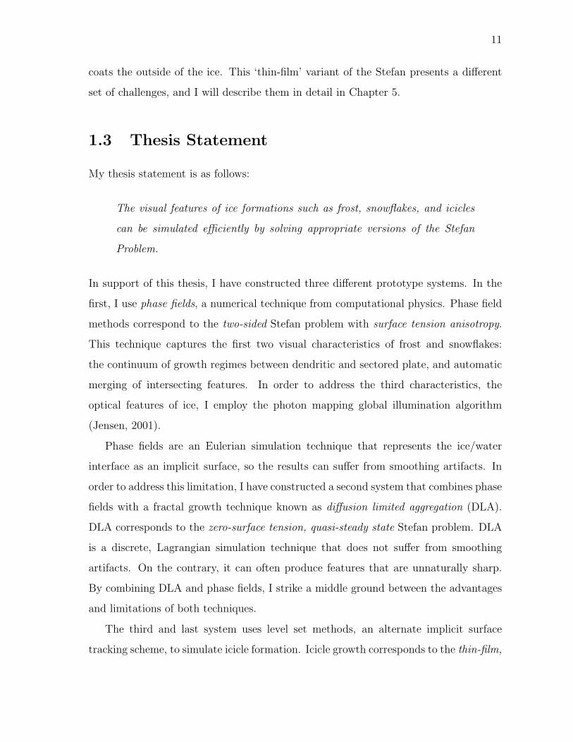
coats the outside of the ice. This ‘thin-film’ variant of the Stefan presents a different

set of challenges, and I will describe them in detail in Chapter 5.

1.3 Thesis Statement

My thesis statement is as follows:

The visual features of ice formations such as frost, snowflakes, and icicles

can be simulated efficiently by solving appropriate versions of the Stefan

Problem.

In support of this thesis, I have constructed three different prototype systems. In the

first, I use phase fields, a numerical technique from computational physics. Phase field

methods correspond to the two-sided Stefan problem with surface tension anisotropy.

This technique captures the first two visual characteristics of frost and snowflakes:

the continuum of growth regimes between dendritic and sectored plate, and automatic

merging of intersecting features. In order to address the third characteristics, the

optical features of ice, I employ the photon mapping global illumination algorithm

(Jensen, 2001).

Phase fields are an Eulerian simulation technique that represents the ice/water

interface as an implicit surface, so the results can suffer from smoothing artifacts. In

order to address this limitation, I have constructed a second system that combines phase

fields with a fractal growth technique known as diffusion limited aggregation (DLA).

DLA corresponds to the zero-surface tension, quasi-steady state Stefan problem. DLA

is a discrete, Lagrangian simulation technique that does not suffer from smoothing

artifacts. On the contrary, it can often produce features that are unnaturally sharp.

By combining DLA and phase fields, I strike a middle ground between the advantages

and limitations of both techniques.

The third and last system uses level set methods, an alternate implicit surface

tracking scheme, to simulate icicle formation. Icicle growth corresponds to the thin-film,

12

quasi-steady state Stefan problem, and the literature on this particular type of Stefan

problem is relatively sparse. There is no established technique akin to phase fields in

the crystal growth literature, so I instead derive the necessary velocity equations for a

level set simulation. The level set solver addresses the first two visual characteristics of

icicles: structures that are longer than they are thick, and merging features. The last

feature, optical effects due to rippling, are addressed by tracking arrival times along

the surface of the icicle. A displacement shader uses these arrival times at render time

to generate ripples using an analytical model from physics.

1.4 Main Results

Beyond capturing the major visual characteristics of a phenomena, there are other

considerations that should be taken into account when constructing a visual simulation

method. For example, it should include intuitive user parameters that can be used to

drive the simulation towards a desired effect, it should be computationally efficient,

and, if possible, it should be easy to implement. With this in mind, the following are

the main results of this dissertation.

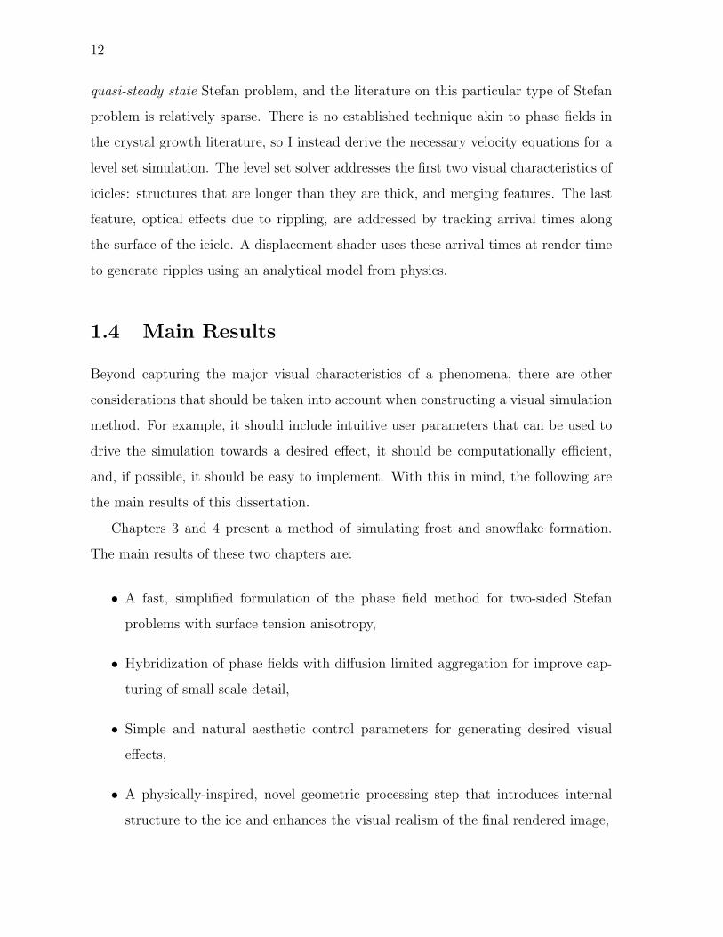
Chapters 3 and 4 present a method of simulating frost and snowflake formation.

The main results of these two chapters are:

• A fast, simplified formulation of the phase field method for two-sided Stefan

problems with surface tension anisotropy,

• Hybridization of phase fields with diffusion limited aggregation for improve cap-

turing of small scale detail,

• Simple and natural aesthetic control parameters for generating desired visual

effects,

• A physically-inspired, novel geometric processing step that introduces internal

structure to the ice and enhances the visual realism of the final rendered image,

13

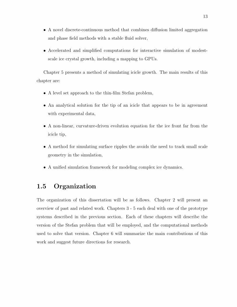
• A novel discrete-continuous method that combines diffusion limited aggregation

and phase field methods with a stable fluid solver,

• Accelerated and simplified computations for interactive simulation of modest-

scale ice crystal growth, including a mapping to GPUs.

Chapter 5 presents a method of simulating icicle growth. The main results of this

chapter are:

• A level set approach to the thin-film Stefan problem,

• An analytical solution for the tip of an icicle that appears to be in agreement

with experimental data,

• A non-linear, curvature-driven evolution equation for the ice front far from the

icicle tip,

• A method for simulating surface ripples the avoids the need to track small scale

geometry in the simulation,

• A unified simulation framework for modeling complex ice dynamics.

1.5 Organization

The organization of this dissertation will be as follows. Chapter 2 will present an

overview of past and related work. Chapters 3 - 5 each deal with one of the prototype

systems described in the previous section. Each of these chapters will describe the

version of the Stefan problem that will be employed, and the computational methods

used to solve that version. Chapter 6 will summarize the main contributions of this

work and suggest future directions for research.

14

Chapter 2

Related Work

The study of pattern formation in solidification spans many different fields, including

math, physics, material science, geology, and computer science. The body of literature

is considerable, with entire journals (e.g. The Journal of Crystal Growth) devoted to

the topic. In this section, I will give a brief a historical perspective, and then survey

the works that are relevant to this dissertation.

2.1 Early Work

As mentioned in the introduction, the study of patterns in ice can be traced back to

at least the 17th century with Kepler and Descartes. However, it was not until the

end of the 19th century, when thermodynamics were better understood, that Stefan

formulated a more quantitative model.

In 1904, Helge von Koch famously described a visual algorithm that captures the

general structure of dendritic ice (von Koch, 1906). It defines simple production rules

that, when applied recursively, produces a structure that is in close visual agreement

with that of a snowflake (Figure 2.1). In contrast to the Stefan problem, the “von Koch

snowflake”, as it is now known, is a discrete model with somewhat tenuous connections

to physical mechanisms. However, due to the simplicity of the algorithm, it is easy to

both understand and analyze, and is often used as the introductory example to fractal

geometry.

16

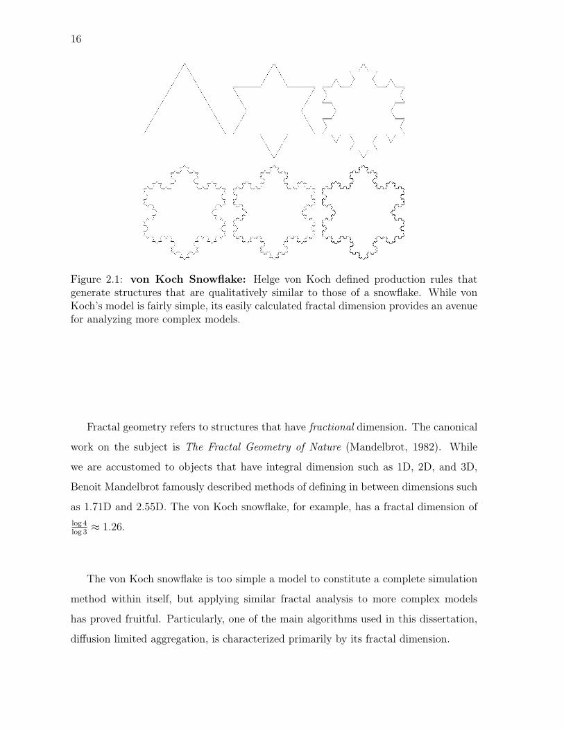
Figure 2.1: von Koch Snowflake: Helge von Koch defined production rules thatgenerate structures that are qualitatively similar to those of a snowflake. While vonKoch’s model is fairly simple, its easily calculated fractal dimension provides an avenuefor analyzing more complex models.

Fractal geometry refers to structures that have fractional dimension. The canonical

work on the subject is The Fractal Geometry of Nature (Mandelbrot, 1982). While

we are accustomed to objects that have integral dimension such as 1D, 2D, and 3D,

Benoit Mandelbrot famously described methods of defining in between dimensions such

as 1.71D and 2.55D. The von Koch snowflake, for example, has a fractal dimension of

log 4log 3

≈ 1.26.

The von Koch snowflake is too simple a model to constitute a complete simulation

method within itself, but applying similar fractal analysis to more complex models

has proved fruitful. Particularly, one of the main algorithms used in this dissertation,

diffusion limited aggregation, is characterized primarily by its fractal dimension.

17

2.2 Related Work In Physics

Wilson “Snowflake” Bentley, a Vermont farmer with no formal scientific training, de-

veloped a technique in 1885 for photographing snowflakes and constructed an extensive

catalog of over 5000 snowflake images. Some of these photographs were later com-

piled and published as a book (Bentley and Humphreys, 1962). Purportedly inspired

by Bentley’s photographs, Japanese physicist Ukichiro Nakaya developed a method of

growing snowflakes in a laboratory, and published an extensive study of crystal shapes

entitled Snow Crystals, Natural and Artificial (Nakaya, 1954). In his book, Nakaya

described a crystal taxonomy and the relationship between crystal shape and atmo-

spheric conditions. Nakaya’s work also gave rise to additional questions, such as why

the transition between different growth regimes was so abrupt.

2.2.1 Phase Field Methods

Addressing solidification problems is difficult for several reasons. The complexity of

crystal structures make them resistent to analytical methods because even the selection

of an appropriate coordinate system becomes difficult. The Stefan problem involves

a free boundary, which means that the equations must be integrated in terms of a

boundary condition that is also one of the unknowns. Finally, there is a jump in physical

values at the ice/water interface, and representing this discontinuity is challenging.

Early methods attempted to simulate solidification using a boundary layer model

(Ben-Jacob et al., 1983; Ben-Jacob et al., 1984), which explicitly tracked the location

of the ice/water interface. While this solves the problem of resolving the ice/water

discontinuity, it can only be used to model very simple crystals, because problems occur

if the interface folds over onto itself. Sethian (Sethian, 1999) describes this problem and

those like it by describing explicit tracking methods as ‘marker and string’ methods. We

can imagine the boundary as represented by a discrete set of marker points, with string

run between adjacent points. During simulation, the markers are moved, and the string

continues to stretch between them. The problem occurs if two of the markers cross over

18

each other, and the string literally becomes tangled. There are various mathematical

methods for untangling or ‘de-looping’ of the results, but they are both inelegant and

extremely difficult to implement.

The phase field method was first suggested by Langer (Langer, 1986) as a model

of solidification. It is an implicit simulation method that does not explicitly track

the location of the ice/water interface. Instead, it addressed the issue of the infinitely

sharp ice/water discontinuity by smearing the interface out into a region of fast but

finite transition that is resolvable on a regular grid. Langer based his work on earlier

work by Halperin et al. (Halperin et al., 1974) and used the term ‘phase field’ that was

coined by Fix (Fix, 1983).

Phase fields were first used to successfully simulate crystal growth of varying mor-

phology by Kobayashi (Kobayashi, 1993), and since then have become the preferred

simulation method in crystal growth. The simulations can be very computationally

expensive however, so various techniques have been applied to the problem. Adaptive

mesh refinement techniques (Provatas et al., 1999) have been used to increase the res-

olution of the solution around regions of interest. Additionally diffusion Monte Carlo

techniques (Plapp and Karma, 2000) have been used to track the heat field far from the

interface, resulting in significant computational savings. Far from the interface, heat is

tracked as a set of particles whose dynamics are much cheaper to compute than flow

over a mesh.

The phase field method is not directly derived from the Stefan problem, but instead

follows from a free energy derivation that appeals more directly to thermodynamics.

As the phase field method composes a significant portion of this dissertation, I will

provide an overview of the derivation here.

While there is more than one method of deriving the phase fields equations, the

most commonly cited one remains the energy derivation from the original paper on

the topic (Langer, 1986). A geometric derivation has also been suggested (Beckermann

et al., 1999), but I will adhere to the energy derivation here. There are several places

in the derivation where different functions can be chosen. In these cases, I will use the

19

choices made by Kobayashi (Kobayashi, 1993), since it is his formulation that is used

in this dissertation.

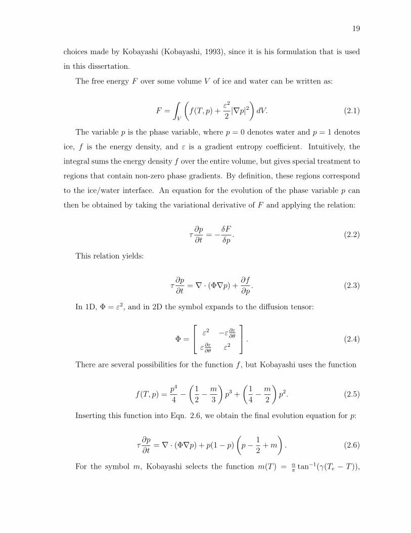
The free energy F over some volume V of ice and water can be written as:

F =

∫

V

(f(T, p) +

ε2

2|∇p|2

)dV. (2.1)

The variable p is the phase variable, where p = 0 denotes water and p = 1 denotes

ice, f is the energy density, and ε is a gradient entropy coefficient. Intuitively, the

integral sums the energy density f over the entire volume, but gives special treatment to

regions that contain non-zero phase gradients. By definition, these regions correspond

to the ice/water interface. An equation for the evolution of the phase variable p can

then be obtained by taking the variational derivative of F and applying the relation:

τ∂p

∂t= −δF

δp. (2.2)

This relation yields:

τ∂p

∂t= ∇ · (Φ∇p) +

∂f

∂p. (2.3)

In 1D, Φ = ε2, and in 2D the symbol expands to the diffusion tensor:

Φ =

ε2 −ε ∂ε

∂θ

ε∂ε∂θ

ε2

. (2.4)

There are several possibilities for the function f , but Kobayashi uses the function

f(T, p) =p4

4−

(1

2− m

3

)p3 +

(1

4− m

2

)p2. (2.5)

Inserting this function into Eqn. 2.6, we obtain the final evolution equation for p:

τ∂p

∂t= ∇ · (Φ∇p) + p(1− p)

(p− 1

2+ m

). (2.6)

For the symbol m, Kobayashi selects the function m(T ) = απ

tan−1(γ(Te − T )),

20

where α, π, and γ are constants, and Te is the freezing temperature of water. Explicitly

multiplying through the diffusion tensor gives the 2D evolution equation:

τ∂p

∂t= ∇ · (ε2∇p)− ∂

∂x

(εε′

∂p

∂y

)+

∂

∂y

(εε′

∂p

∂x

)+ p(1− p)

(p− 1

2+ m

). (2.7)

Subsequent work has rigorously proved that in the limit, limε→0 τ ∂p∂t

, the phase field

equations do indeed converge to the Stefan problem with surface tension (Caginalp and

Chen, 1992).

2.2.2 Level Set Methods

Level set methods, an alternate implicit front tracking strategy, has also been success-

ful in simulating crystal formation. Level set methods were first developed by Osher

and Sethian (Osher and Sethian, 1988) as a general front tracking strategy, and have

since found numerous applications including computational fluid dynamics (Foster and

Metaxas, 1996), lithography (Adalsteinsson and Sethian, 1995b; Adalsteinsson and

Sethian, 1995c; Adalsteinsson and Sethian, 1997), and computer vision (Malladi et al.,

1995). Both Osher (Osher and Fedkiw, 2003) and Sethian (Sethian, 1999) have written

books that exhaustively describe level set methods, the wide variety of techniques that

have been developed surrounding them, and their numerous applications.

Whereas phase fields smear out the location of the ice/water interface, level set

methods track the precise position of this interface. Instead of tracking a phase order

parameter p, the level set method tracks the evolution of some implicit function φ,

usually a signed distance function. Whereas the phase field method essentially relies

on a reaction equation to correctly evolve the interface, level set methods construct a

velocity field v over the entire computational domain and then evolve φ according to

∂φ

∂t+ v · ∇φ = 0.

21

The nomenclature of phase field and level set methods can unfortunately overlap,

because in a general sense ‘level sets’ refer to the isosurface of an implicit function.

Therefore the interface location in phase fields is sometimes referred to as the ‘0.5 level

set’ or the ‘zero level set’, depending on if the p parameter is defined over [0,1] or [-1,1].

To avoid confusion, I will only use the term ‘level set’ in this dissertation when referring

to the level set method.

Since phase fields only converge to the Stefan problem in the limit, it has been

argued that they are only a first order accurate tracking method (Gibou et al., 2003).

Level set methods were first applied to the problem of solidification in by Sethian

and Strain (Sethian and Strain, 1992) using a boundary integral approach. A simpler

method was later suggested by Chen et. al. (Chen et al., 1997) and later extended in

a pair of articles (Gibou et al., 2003; Gibou and Fedkiw, 2005) to second and fourth

order accuracy.

The strategy followed level set simulation of the Stefan problem is slightly different

from that of the phase field method. While both use an implicit function to track the

interface, the level set approach essentially constructs a temporary explicit represen-

tation every timestep. Since the implicit function used is a signed distance function

instead of a phase order parameter, it is possible to locate the explicit interface with

much higher accuracy than in phase field methods. Once this is done, the boundary is

set according to the the Gibbs-Thomson relation,

TI = εcκ− εvVn

where TI is the temperature at the interface, εc is a surface tension coefficient, κ is the

local curvature, εv is the molecular kinetic coefficient, and Vn is the normal velocity of

the interface.

Once these quantities have been defined along the interface, they must be incor-

porated back into the implicit level set simulation. A problem arises here because the

Gibbs-Thomson relation only defines velocities along the ice/water interface, while level

22

set simulator require a velocity to be defined over the entire computational domain.

This problem is overcome by interpolating the computed interface velocities back into

their corresponding grid cells, and then extending the values over the entire simulation

domain using an extension velocities method (Adalsteinsson and Sethian, 1999).

While the level set approach does yield higher numerical accuracy, it utilizes a good

deal more numerical machinery than the phase field method. For simplicity, I use the

phase field method in chapters 3 and 4. However, for the case of icicle growth, some of

the features of level set methods become necessary, so I use them in chapter 5.

2.2.3 Thin Film Growth

All of the above work deals with growth in the presence of a large water supply. The

previous work in phase fields and level set methods assume that the crystal is growing

in an infinite bath of supercooled water, and Nakaya’s snowflake work assumes that a

large supply of water vapor is present in the atmosphere. Icicle growth instead deals

with the case where the water supply is severely limited.

In glaciology, there exists some work on the problem of thin-film ice growth. Several

analytical models exist for icicle formation (Maeno et al., 1994; Makkonen, 1988; Szilder

and Lozowski, 1994), but these models are concerned with accurately capturing the

ratio of an icicle’s length to its radius. These models are derived using an energy

balance approach using a plethora of environmental variables that are of limited value

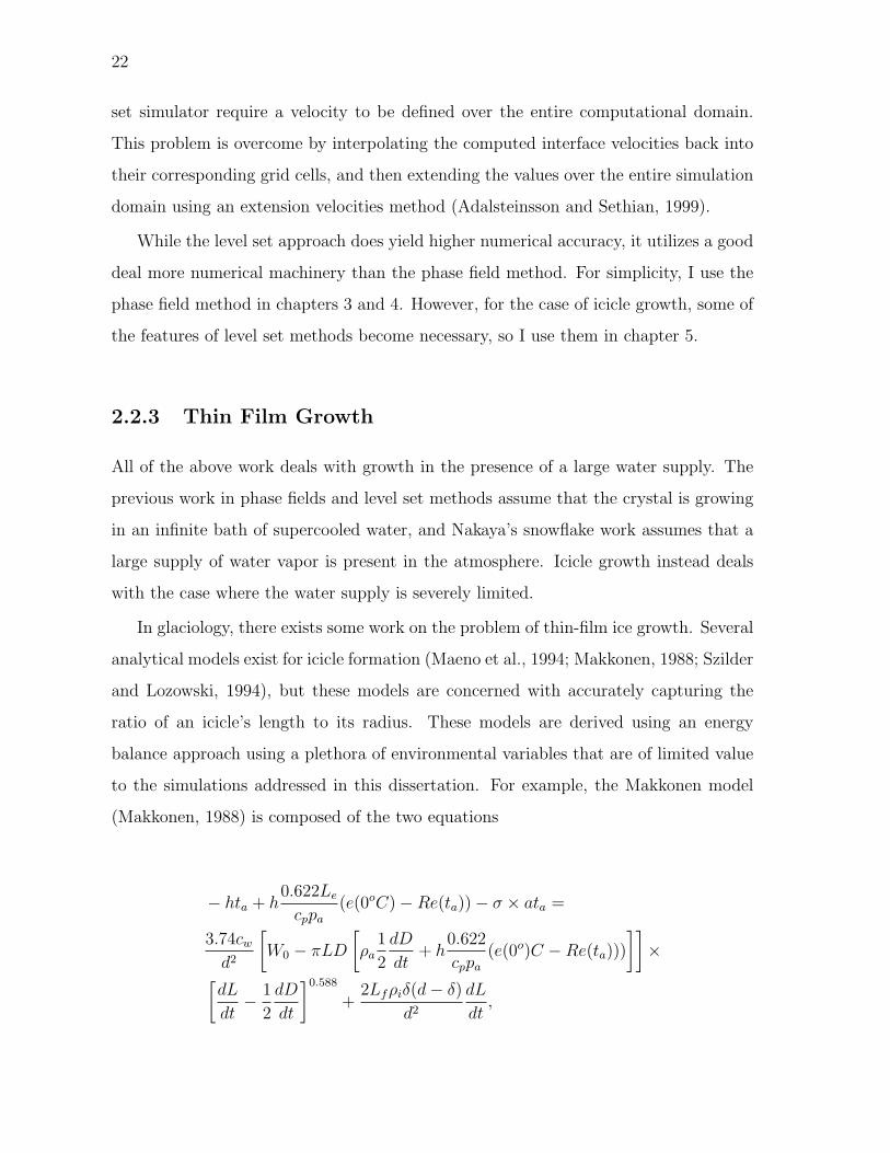
to the simulations addressed in this dissertation. For example, the Makkonen model

(Makkonen, 1988) is composed of the two equations

− hta + h0.622Le

cppa

(e(0oC)−Re(ta))− σ × ata =

3.74cw

d2

[W0 − πLD

[ρa

1

2

dD

dt+ h

0.622

cppa

(e(0o)C −Re(ta)))

]]×

[dL

dt− 1

2

dD

dt

]0.588

+2Lfρiδ(d− δ)

d2

dL

dt,

23

symbol definition

h convective heat-transfer coefficientta air temperatureLe latent heat of evaporationcp specific heat of waterpa air pressure

e(0oC) saturation water-vapor pressureR Relative humidity

e(ta) saturation water-vapor pressureσ Stefan-Boltzmann constantd diameter of pendant drop

W0 mass flux of water to tipρa density of icicle wallsρi ice densityδ wall thickness at tip

Table 2.1: Symbols for the Makkonen (Makkonen, 1988) model.

and

dD

dt=−hwta + hw

0.622Le

cppa[e(0o)C −Re(ta)]− σata

12ρaLf (1− λ)

.

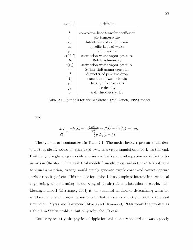
The symbols are summarized in Table 2.1. The model involves pressures and den-

sities that ideally would be abstracted away in a visual simulation model. To this end,

I will forgo the glaciology models and instead derive a novel equation for icicle tip dy-

namics in Chapter 5. The analytical models from glaciology are not directly applicable

to visual simulation, as they would merely generate simple cones and cannot capture

surface rippling effects. Thin film ice formation is also a topic of interest in mechanical

engineering, as ice forming on the wing of an aircraft is a hazardous scenario. The

Messinger model (Messinger, 1953) is the standard method of determining when ice

will form, and is an energy balance model that is also not directly applicable to visual

simulation. Myers and Hammond (Myers and Hammond, 1999) recast the problem as

a thin film Stefan problem, but only solve the 1D case.

Until very recently, the physics of ripple formation on crystal surfaces was a poorly

24

understood phenomena. However, Ogawa and Furukawa (Ogawa and Furukawa, 2002)

recently proposed a model of ripple formation which was subsequently refined by Ueno

in a pair of articles (Ueno, 2003; Ueno, 2004). The former model only applies to a

cylinder, and the latter model was derived for an inclined plane. Ueno’s model will

later be used in Chapter 5 to simulate ripple formation along the surface of an icicle.

2.2.4 Laplacian Growth

Laplacian growth is a general class of physical phenomena that includes ice growth,

lightning formation, liquid surface tension, quasi-steady state fracture, and river for-

mation, among others. The unifying notion is that patterns form according to a field

that satisfies the Laplace equation (Eqn. 1.5). In the case of ice formation, this field

corresponds to a quasi-steady state heat field. In other phenomena, the correspondence

differs. In lightning and surface tension for example, the field corresponds to electric

potential and fluid pressure.

A Laplacian growth simulation technique that has received a good deal of attention

in the physics literature is diffusion limited aggregation, usually abbreviated as DLA

(Witten and Sander, 1981). Originally formulated as a model of aggregating metal

particles, it has since found success in various other phenomena, including snowflake

growth (Family et al., 1987; Nittmann and Stanley, 1987). One of the defining charac-

teristics of DLA is that it produces fractal structures. In 2D, DLA produces structures

of approximately D ≈ 1.71, and in 3D, D ≈ 2.55.

The DLA algorithm is simple enough that it can be described informally. Given a

discrete 2D grid, a single particle representing the crystal (or ‘aggregate’) is placed in

the center. A particle called the ‘walker’ is then placed at a random location along the

grid perimeter. The particle walks randomly along adjacent grid cells until it either

is adjacent to the crystal or falls off the grid. If it is adjacent to the crystal, it sticks

and becomes part of the crystal. A new walker is then inserted at the perimeter and

the random walk is repeated. The process repeats until the desired aggregate size is

achieved.

25

At first glance, it is not obvious that DLA corresponds to a Stefan problem, as

it does not involve any differential equations. However, there are several algorithms

that generate results that are visually indistinguishable from the results of DLA. One of

these algorithms, the dielectric breakdown model (DBM) (Niemeyer et al., 1984) utilizes

the Laplace equation (Eqn. 1.5) where DLA uses a random walk. I will later use DBM

in Chapter 4 to describe the relationship of DLA to a Stefan problem.

2.3 Analytical Solutions to the Stefan Problem

There are a handful of known analytical solutions to the Stefan problem, and they only

apply over simple geometries. However, I will use these solutions and their derivations

later in chapter 5 to derive thin-film equivalents, so I will describe the classical ‘infinite

water’ derivations here.

2.3.1 Planar Case

The planar case of the Stefan problem involves one coordinate, usually denoted as

the negative z direction. This is because Stefan originally formulated the problem in

terms of ocean ice forming, and the ice forms first at the surface of the water and

gradually thickens downwards into an infinitely deep ocean. There are several different

approaches to solving the 1D equations, but I will use the ‘moving-frame’ approach

described in Saito (Saito, 1996). In this case we assume that the global coordinate is

z, but introduce a moving variable z′ = z − V t, where V is velocity and t is time. In

this way, at any time t, z′ = 0 denotes the current location of the interface. In terms

of this moving frame, the diffusion equation becomes

1

D

∂T

∂t= ∇2T +

2

lD

∂T

∂z′

where D is again the thermal diffusion constant and lD = 2DV

. Applying the quasi-

steady state approximation, we obtain

26

∇2T +2

lD

∂T

∂z′= 0.

By specifying an infinitely far away boundary condition T (z′ = ∞) = 0, this can

be integrated to

T (z′) = Ae− 2z′

lD ,

where A is an as yet undetermined constant of integration. The second equation in the

1D Stefan problem can now be written as:

dz′

dt= −D

dT

dz.

In this form, it can be solved by plugging in the T (z′) to obtain:

dz′

dt= −D

2A

lD= AV.

Since V = dz′dt

, this means that the constant A must be equal to 1. We then apply

the Wilson-Frenkel law:

dz′

dt= K((Tu)− Ti − dκ),

where K is the kinetic coefficient, Tu is the undercooling of the water, Ti is the tem-

perature at the interface, d is the capillary length, and κ is the curvature. Applying

this to the velocity equation, we obtain the final velocity of the planar interface:

dz′

dt= K(Tu − 1).

The feature to note is that this value is a constant, so for the planar case, the

ice/water interface advances at a uniform velocity.

27

2.3.2 Spherical Case

The case of a sphere was solved by Frank (Frank, 1949), and is thus sometimes referred

to as the ‘Frank sphere’ case. Again, I follow the derivation given by Saito (Saito,

1996). The case is again 1D, but instead of the cartesian coordinate z, we have the

radial coordinate r, and the moving frame is r′ instead of z′. The diffusion equation in

spherical coordinates is:

1

D

∂T

∂t=

(∂2

∂r2+

2

r

∂

∂r

)T.

Again applying the quasi-steady state approximation, we obtain:

(∂2

∂r2+

2

r

∂

∂r

)T = 0.

Similar to the planar case, we specify an infinitely far away boundary condition

T (r′ = ∞) = 0, and obtain the solution T (r) = Ar. A is again an undetermined constant

of integration. Applying the second equation of the Stefan problem, we obtain:

dr′

dt=

DA

(r′)2.

Again applying the Wilson-Frenkel law, we obtain:

dr′

dt= K

(Tu − A

r′− 2d

r′

).

Using these two equations, the constant of integration A is uniquely determined as:

A =(r′)2

(Tu − 2d

r′)

r′ + DK

.

The final velocity equation is then:

dr′

dt=

D(Tu − 2d

r′)

r′ + DK

.

The detail to note is that below a certain radius, 2dTu

, the sphere will not grow. Unlike

28

the planar case, when the sphere does grow, it does not have a constant velocity, and

instead the velocity slows as the radius increases.

2.3.3 Parabolic Case

In the parabolic case, we assume that the growing crystal takes the form of a parabola,

and obtain an expression for the velocity of the tip. The original solution was obtained

by Ivantsov (Ivantsov, 1947), but again I follow the derivation in Saito (Saito, 1996).

To characterize the position of the tip, we use the same z and z′ coordinates from the

planar case, but in this case z′ denotes the location of a parabola tip, not a plane. We

then define a parabolic coordinate system around the z axis:

ξ = r − z′

η = r + z′

θ = arctan(x/y).

In this case, r is defined as r =√

x2 + y2 + (z′)2. The parabolic version of the

quasi-steady state heat equation can be written as:

1

η + ξ

(∂

∂ηη∂T

∂η+

∂

∂ξξ∂T

∂ξ

)+

1

4ηξ

∂2T

∂θ2+

1

lD

1

η + ξ

(η∂T

∂η− ξ

∂T

∂ξ

)= 0.

If we assume circular symmetry, this reduces to:

∂

∂η

(η∂T

∂η

)+

1

lD

(η∂T

∂η

)= 0.

Denoting the current location of the interface as ηi, the second equation of the

Stefan problem translates to:

ηi + ξ∂ηi

∂ξ+

ηi + ξ

2V

∂ηi

∂t= −lD

(ηi

∂u

∂η− ξ

∂ηi

∂ξ

∂T

∂ξ− ηi + ξ

4ηiξ

∂ηi

∂θ

∂T

∂θ

).

29

Using the boundary condition T (ηi) = Tu, the temperature field integrates to:

T (η) = Tu + C

∫ η

R

e− x

lD

xdx.

The symbol R denotes the radius of curvature of the parabola tip and C is a constant

of integration. Using the boundary condition T (η = ∞) = 0, we can solve for the value

of C,

C = − Tu

∫∞R

e− x

lD

xdx

,

and obtain the heat solution:

T (η) = Tu

1−

∫ η

Re− x

lD

xdx

∫∞R

e− x

lD

xdx

.

Inserting this heat solution into the second equation of the Stefan problem, we

obtain what is known as the ‘Ivantsov relation’:

Tu =R

lDe

RlD

∫ ∞

R

e− x

lD

x.

The relation is usually simplified using the change of variables P = RlD

and expo-

nential notation E1(P ) =∫∞

Pe−x

xto obtain:

Tu = PeP E1(P ). (2.8)

For small undercoolings, this relation is sometimes approximated in 3D as Tu ≈P (− log P − γ), where γ is the Euler-Mascheroni constant, and in 2D as Tu ≈

√πP .

The feature to note is that the Ivantsov relation is that given an undercoooling

Tu, it can only be solved for the product of the radius of curvature and the velocity,

RV . The tip velocity, the quantity that we are looking for, cannot be solved for

directly. Experimental data shows that tip velocities are uniquely determined by the

undercooling however, suggesting that an additional constraint is missing.

30

A good deal of effort has been devoted to determining the nature of this additional

constraint. ‘Microscopic solvability theory’ (see for example (Brener and Mel‘nikov,

1991)) suggests that the missing constraint is surface tension. Fortunately, in the

case of icicle growth, experimental measurements show that the radius of the icicle tip

stays relatively stationary under a wide variety of undercoolings, so in the case of this

dissertation, an appeal to microscopic solvability theory is unnecessary.

2.3.4 Cylindrical Case

The cylindrical case corresponds to the case where a small column of undercooled water

is surrounded by ice. I will follow the derivation given by Hill (Hill, 1987) here. The

heat equation in cylindrical coordinates is:

∂T

∂t= D

(∂2T

∂r2+

1

r

∂T

∂r+

1

r2

∂2T

∂θ2+

∂2T

∂y2

).

Applying the quasi-steady state approximation and assuming homogeneity in all

but the radial direction, this reduces to:

∂2T

∂r2+

1

r

∂T

∂r= 0.

The solution must be of the form

T (r, t) = A + B log r.

As before, the interface r′ is constrained to the freezing temperature Tf , but instead

of applying the Wilson-Frenkel law at the interface, we apply Newton cooling:

T (1, t) + β∂T (1, r)

∂r= 1.

In terms of the unknowns these constraints translate to:

31

A + B log 1 + βB

1= A + βB = 1

A + B log r′ = Tf .

We can then solve for A and B:

A = −(1− Tf ) log r′

β − log r′

B =1− Tf

β − log r′

Thus the heat field solves to:

T (r, t) =log r − (1− Tf ) log r′

β − log r′

Inserting this into the second equation of the Stefan problem yields:

dr′

dt= −D

∂T

∂r′=

−D

r′(β − log r′).

This equation can be integrated if first inverted,

dt

dr′=−r′(β − log r′)

D,

and then integrated with respect to r′ to get an ‘arrival time’ equation:

t(r′) =1

4D(2(r′)2 log r′ − (1 + 2β)(1− (r′)2)).

The identity∫

x log x dx = x2

2(log x− 1

2) was applied in order to perform this inte-

gration. Intuitively, this equation describes the time at which the interface will arrive

at some radius r′. Instead of performing this final integration, I will later use a thin-film

variant of the dr′dt

equation, because this form is better suited for a level set simulation.

32

2.4 Related Work In Graphics

2.4.1 Phase Transition

Phase transition is a relatively new topic in computer graphics, because until recently,

robust, efficient solvers for objects of a single state were not commonly available.

Clearly, it would be difficult to simulate an object transitioning from solid to liquid

in the absence of robust rigid body and fluid simulators.

In particular, recent techniques used for fluid simulation are relevant to this disser-

tation, since I use many of the same techniques to track the rapidly evolving ice surface.

Early work in fluid simulation solved the Navier-Stokes equations using the Marker-In-

Cell (MAC) method (Foster and Metaxas, 1996) from computational fluid dynamics

(Harlow and Welch, 1966), and also efficiently solved the shallow water equations (Kass

and Miller, 1990).

In his seminal 1999 paper, Stam described a fast, unconditionally stable method of

simulating the Navier-Stokes equations (Stam, 1999b). Subsequently, considerable re-

search effort has been devoted to building on Stam’s ideas and formulating alternative

approaches. Free boundaries were added to take into account pouring and splashing

(Enright et al., 2002b; Foster and Fedkiw, 2001), and the concept of ‘vorticity con-

finement’ was introduced to counteract numerical smearing (Fedkiw et al., 2001). An

efficient method of simulating smoke and water on an octree data structure was also

introduced (Losasso et al., 2004). I will later use similar techniques for icicle simulation.

With this increased interest in fluid simulation, the problem of phase transition

has also received attention. Carlson et al. (Carlson et al., 2002) presented a MAC

method of simulating variable viscosity fluids which could handle situations such as

wax melting. The key idea was to treat solid objects as liquids with very high viscosity,

and a similar approach was taken in later work (Carlson et al., 2004) to simulate the

interaction of rigid objects with fluid. Alternatively, Wei et al. (Wei et al., 2003)

presented a Lattice-Boltzmann based methods for simulating melting. Subsequently,

Rasmussen et al. (Rasmussen et al., 2004) described an IMEX scheme for the viscous

33

forcing terms involved in melting simulations, and Losasso et al. (Losasso et al., 2005)

described a method of melting Lagrangian solids into Eulerian liquids.

Other work has also dealt with visco-elastic objects that possess viscosities much

higher than water, but still exhibit flowing behavior (Goktekin et al., 2004; Clavet

et al., 2005). These works do not appear to handle large viscosity transitions however,

so the methods are not directly applicable to solidification.

2.4.2 Modeling Winter Scenes

The problem of modeling a winter scene has received attention in graphics because it

gives rise to a unique set of challenges. Fallen snow has a specific geometric shape that

cannot be captured by simply offsetting existing scene geometry. More sophisticated,

physically-based approaches have been attempted such as the use of metaballs (Nishita

et al., 1997), and a ‘visible sky’ algorithm (Fearing, 2000) that is similar to the ambient

occlusion algorithm in global illumination. Recent work has also successfully modeled

the appearance of snow falling from the sky (Langer et al., 2004).

Modeling ice formation in these scenes has not been as closely examined. To my

knowledge, the only work that bears some resemblance to that presented here is by

Kharitonsky and Gonczarowski (Kharitonsky and Gonczarowski, 1993). They de-

scribed a random-walk model of icicle growth, where water droplets walk along an

ice surface and freeze with a certain probability. However, their approach does not

naturally handle the formation of more than one icicle. More seriously, the notion that

icicles form as the aggregate of discrete droplets is not empirically supported.

2.4.3 Pattern Formation

While the specific goal of this dissertation is the modeling of ice formations, in a

more general sense, the problem of solidification is one of pattern formation. Formally,

physicists define pattern formation as when “nonlinearities conspire to form spatial

patterns that sometimes are stationary, travelling or disordered in space and time.”

34

(Bodenschatz et al., 2003). In this sense, the work in this dissertation is one of many

pattern formation algorithms in computer graphics. The patterns that form in fluid

simulation, for example, fall into this category due to the non-linear advection term.

Visual phenomena that arise as a consequence of flow, such as sand dunes and rust

patterns (Dorsey et al., 1996; Chen et al., 2005) meet this criteria as well.

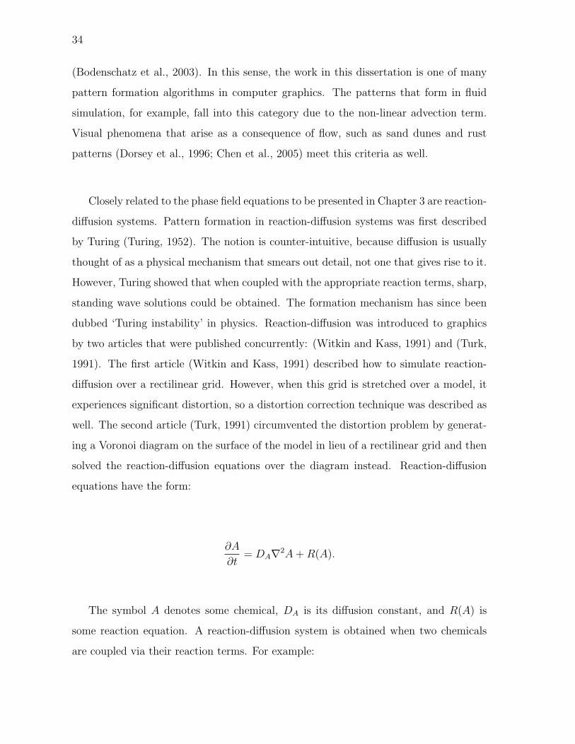
Closely related to the phase field equations to be presented in Chapter 3 are reaction-

diffusion systems. Pattern formation in reaction-diffusion systems was first described

by Turing (Turing, 1952). The notion is counter-intuitive, because diffusion is usually

thought of as a physical mechanism that smears out detail, not one that gives rise to it.

However, Turing showed that when coupled with the appropriate reaction terms, sharp,

standing wave solutions could be obtained. The formation mechanism has since been

dubbed ‘Turing instability’ in physics. Reaction-diffusion was introduced to graphics

by two articles that were published concurrently: (Witkin and Kass, 1991) and (Turk,

1991). The first article (Witkin and Kass, 1991) described how to simulate reaction-

diffusion over a rectilinear grid. However, when this grid is stretched over a model, it

experiences significant distortion, so a distortion correction technique was described as

well. The second article (Turk, 1991) circumvented the distortion problem by generat-

ing a Voronoi diagram on the surface of the model in lieu of a rectilinear grid and then

solved the reaction-diffusion equations over the diagram instead. Reaction-diffusion

equations have the form:

∂A

∂t= DA∇2A + R(A).

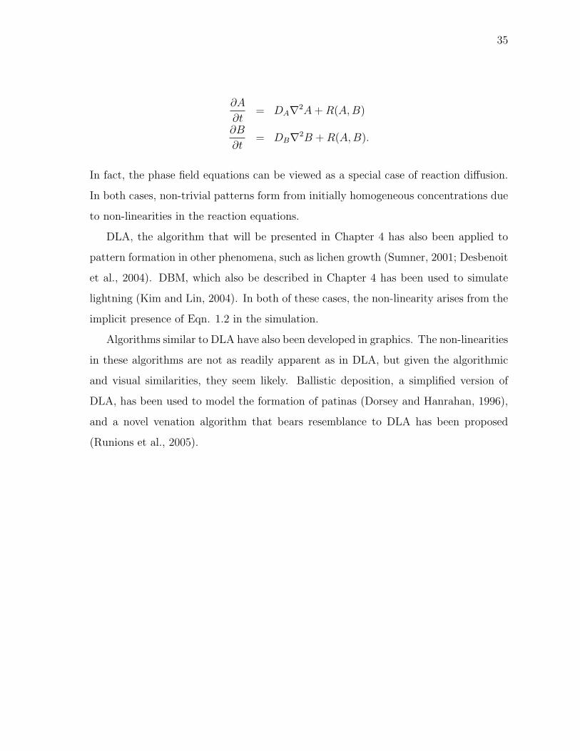
The symbol A denotes some chemical, DA is its diffusion constant, and R(A) is

some reaction equation. A reaction-diffusion system is obtained when two chemicals

are coupled via their reaction terms. For example:

35

∂A

∂t= DA∇2A + R(A,B)

∂B

∂t= DB∇2B + R(A,B).

In fact, the phase field equations can be viewed as a special case of reaction diffusion.

In both cases, non-trivial patterns form from initially homogeneous concentrations due

to non-linearities in the reaction equations.

DLA, the algorithm that will be presented in Chapter 4 has also been applied to

pattern formation in other phenomena, such as lichen growth (Sumner, 2001; Desbenoit

et al., 2004). DBM, which also be described in Chapter 4 has been used to simulate

lightning (Kim and Lin, 2004). In both of these cases, the non-linearity arises from the

implicit presence of Eqn. 1.2 in the simulation.

Algorithms similar to DLA have also been developed in graphics. The non-linearities

in these algorithms are not as readily apparent as in DLA, but given the algorithmic

and visual similarities, they seem likely. Ballistic deposition, a simplified version of

DLA, has been used to model the formation of patinas (Dorsey and Hanrahan, 1996),

and a novel venation algorithm that bears resemblance to DLA has been proposed

(Runions et al., 2005).

36

Chapter 3

The Phase Field Method

In this chapter, I describe one method of solving the Stefan problem, the phase field

method. The general approach of the phase field method was derived independent of

the Stefan problem, using an approach that appeals more directly to thermodynamics.

A summary of this free energy approach is available in the previous chapter. I will

provide an overview of the phase field equations and describe how they intuitively map

to the Stefan problem.

Additionally, I present techniques to simplify the phase field computation and make

the problem of simulating ice crystal growth more tractable. I also show how the phase

field method allows a user parameterization that a visual effects artist can use to manip-

ulate the ice crystal growth. The phase field method often has smoothing artifacts as a

result of its implicit representation, and it can only compute the outermost ice/water

boundary. Therefore, a novel intermediate geometric processing step is introduced to

add sharp edges and medial ridges to the interior of the ice. Finally, the simulated

images are rendered using photon mapping (Jensen, 2001).

The basic simulation and rendering framework has been applied to several different

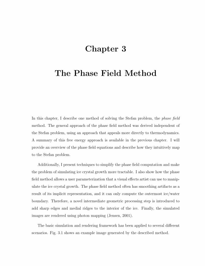
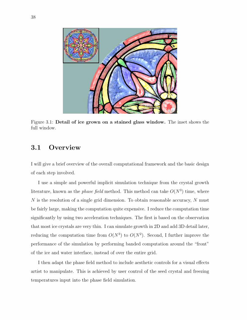
scenarios. Fig. 3.1 shows an example image generated by the described method.

38

Figure 3.1: Detail of ice grown on a stained glass window. The inset shows thefull window.

3.1 Overview

I will give a brief overview of the overall computational framework and the basic design

of each step involved.

I use a simple and powerful implicit simulation technique from the crystal growth

literature, known as the phase field method. This method can take O(N3) time, where

N is the resolution of a single grid dimension. To obtain reasonable accuracy, N must

be fairly large, making the computation quite expensive. I reduce the computation time

significantly by using two acceleration techniques. The first is based on the observation

that most ice crystals are very thin. I can simulate growth in 2D and add 3D detail later,

reducing the computation time from O(N3) to O(N2). Second, I further improve the

performance of the simulation by performing banded computation around the “front”

of the ice and water interface, instead of over the entire grid.

I then adapt the phase field method to include aesthetic controls for a visual effects

artist to manipulate. This is achieved by user control of the seed crystal and freezing

temperatures input into the phase field simulation.

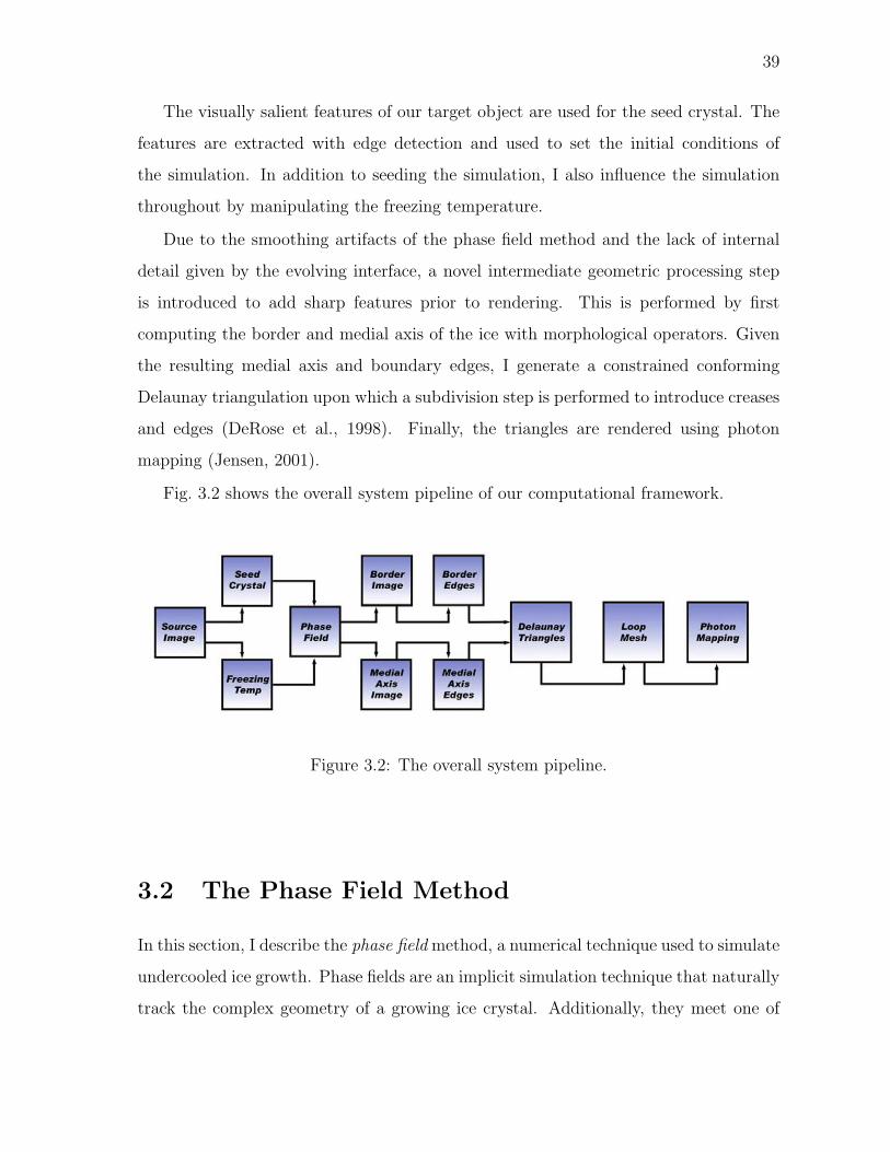
39

The visually salient features of our target object are used for the seed crystal. The

features are extracted with edge detection and used to set the initial conditions of

the simulation. In addition to seeding the simulation, I also influence the simulation

throughout by manipulating the freezing temperature.

Due to the smoothing artifacts of the phase field method and the lack of internal

detail given by the evolving interface, a novel intermediate geometric processing step

is introduced to add sharp features prior to rendering. This is performed by first

computing the border and medial axis of the ice with morphological operators. Given

the resulting medial axis and boundary edges, I generate a constrained conforming

Delaunay triangulation upon which a subdivision step is performed to introduce creases

and edges (DeRose et al., 1998). Finally, the triangles are rendered using photon

mapping (Jensen, 2001).

Fig. 3.2 shows the overall system pipeline of our computational framework.

Figure 3.2: The overall system pipeline.

3.2 The Phase Field Method

In this section, I describe the phase field method, a numerical technique used to simulate

undercooled ice growth. Phase fields are an implicit simulation technique that naturally

track the complex geometry of a growing ice crystal. Additionally, they meet one of

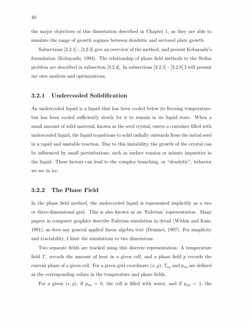
40

the major objectives of this dissertation described in Chapter 1, as they are able to

simulate the range of growth regimes between dendritic and sectored plate growth.

Subsections [3.2.1] - [3.2.3] give an overview of the method, and present Kobayashi’s

formulation (Kobayashi, 1993). The relationship of phase field methods to the Stefan

problem are described in subsection [3.2.4]. In subsections [3.2.5] - [3.2.8] I will present

my own analysis and optimizations.

3.2.1 Undercooled Solidification

An undercooled liquid is a liquid that has been cooled below its freezing temperature,

but has been cooled sufficiently slowly for it to remain in its liquid state. When a

small amount of solid material, known as the seed crystal, enters a container filled with

undercooled liquid, the liquid transitions to solid radially outwards from the initial seed

in a rapid and unstable reaction. Due to this instability, the growth of the crystal can

be influenced by small perturbations, such as surface tension or minute impurities in

the liquid. These factors can lead to the complex branching, or “dendritic”, behavior

we see in ice.

3.2.2 The Phase Field

In the phase field method, the undercooled liquid is represented implicitly as a two

or three-dimensional grid. This is also known as an ‘Eulerian’ representation. Many

papers in computer graphics describe Eulerian simulation in detail (Witkin and Kass,

1991), as does any general applied linear algebra text (Demmel, 1997). For simplicity

and tractability, I limit the simulations to two dimensions.

Two separate fields are tracked using this discrete representation: A temperature

field T , records the amount of heat in a given cell, and a phase field p records the

current phase of a given cell. For a given grid coordinate (x, y), Txy and pxy are defined

as the corresponding values in the temperature and phase fields.

For a given (x, y), if pxy = 0, the cell is filled with water, and if pxy = 1, the

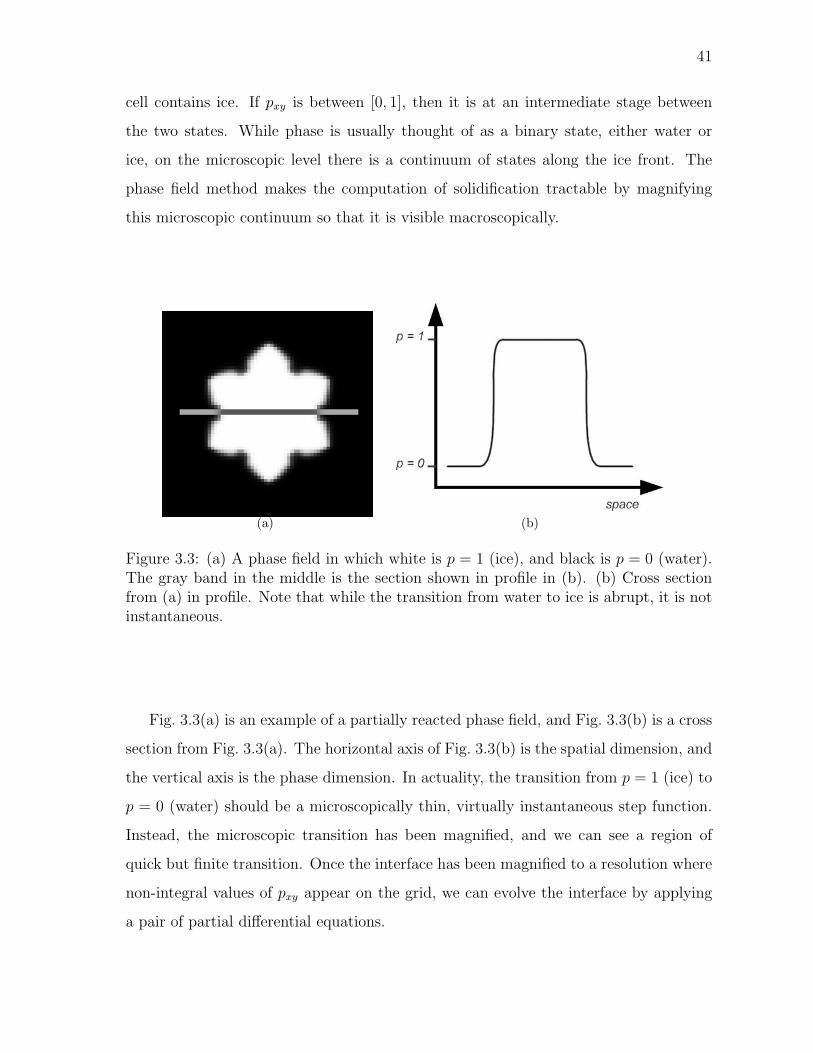
41

cell contains ice. If pxy is between [0, 1], then it is at an intermediate stage between

the two states. While phase is usually thought of as a binary state, either water or

ice, on the microscopic level there is a continuum of states along the ice front. The

phase field method makes the computation of solidification tractable by magnifying

this microscopic continuum so that it is visible macroscopically.

(a) (b)

Figure 3.3: (a) A phase field in which white is p = 1 (ice), and black is p = 0 (water).The gray band in the middle is the section shown in profile in (b). (b) Cross sectionfrom (a) in profile. Note that while the transition from water to ice is abrupt, it is notinstantaneous.

Fig. 3.3(a) is an example of a partially reacted phase field, and Fig. 3.3(b) is a cross

section from Fig. 3.3(a). The horizontal axis of Fig. 3.3(b) is the spatial dimension, and

the vertical axis is the phase dimension. In actuality, the transition from p = 1 (ice) to

p = 0 (water) should be a microscopically thin, virtually instantaneous step function.

Instead, the microscopic transition has been magnified, and we can see a region of

quick but finite transition. Once the interface has been magnified to a resolution where

non-integral values of pxy appear on the grid, we can evolve the interface by applying

a pair of partial differential equations.

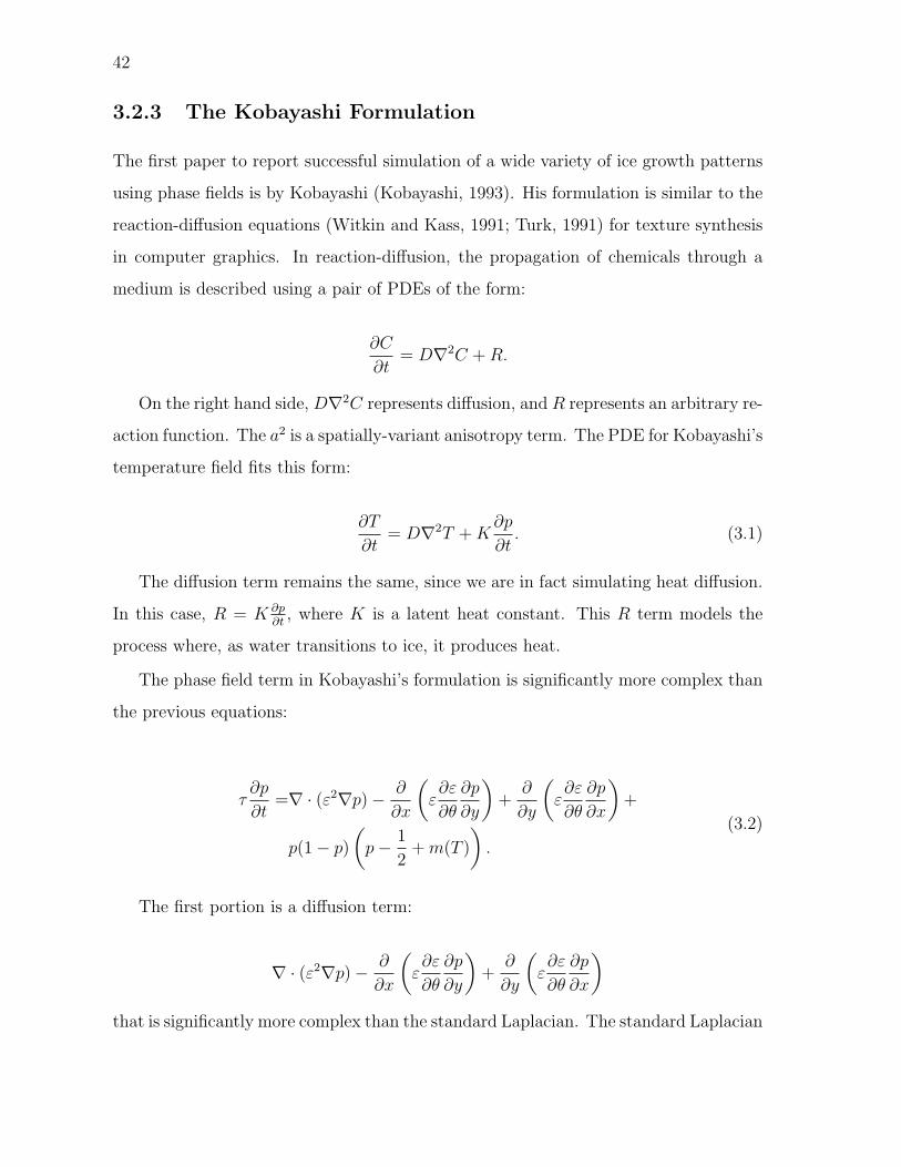
42

3.2.3 The Kobayashi Formulation

The first paper to report successful simulation of a wide variety of ice growth patterns

using phase fields is by Kobayashi (Kobayashi, 1993). His formulation is similar to the

reaction-diffusion equations (Witkin and Kass, 1991; Turk, 1991) for texture synthesis

in computer graphics. In reaction-diffusion, the propagation of chemicals through a

medium is described using a pair of PDEs of the form:

∂C

∂t= D∇2C + R.

On the right hand side, D∇2C represents diffusion, and R represents an arbitrary re-

action function. The a2 is a spatially-variant anisotropy term. The PDE for Kobayashi’s

temperature field fits this form:

∂T

∂t= D∇2T + K

∂p

∂t. (3.1)

The diffusion term remains the same, since we are in fact simulating heat diffusion.

In this case, R = K ∂p∂t

, where K is a latent heat constant. This R term models the

process where, as water transitions to ice, it produces heat.

The phase field term in Kobayashi’s formulation is significantly more complex than

the previous equations:

τ∂p

∂t=∇ · (ε2∇p)− ∂

∂x

(ε∂ε

∂θ

∂p

∂y

)+

∂

∂y

(ε∂ε

∂θ

∂p

∂x

)+

p(1− p)

(p− 1

2+ m(T )

).

(3.2)

The first portion is a diffusion term:

∇ · (ε2∇p)− ∂

∂x

(ε∂ε

∂θ

∂p

∂y

)+

∂

∂y

(ε∂ε

∂θ

∂p

∂x

)

that is significantly more complex than the standard Laplacian. The standard Laplacian

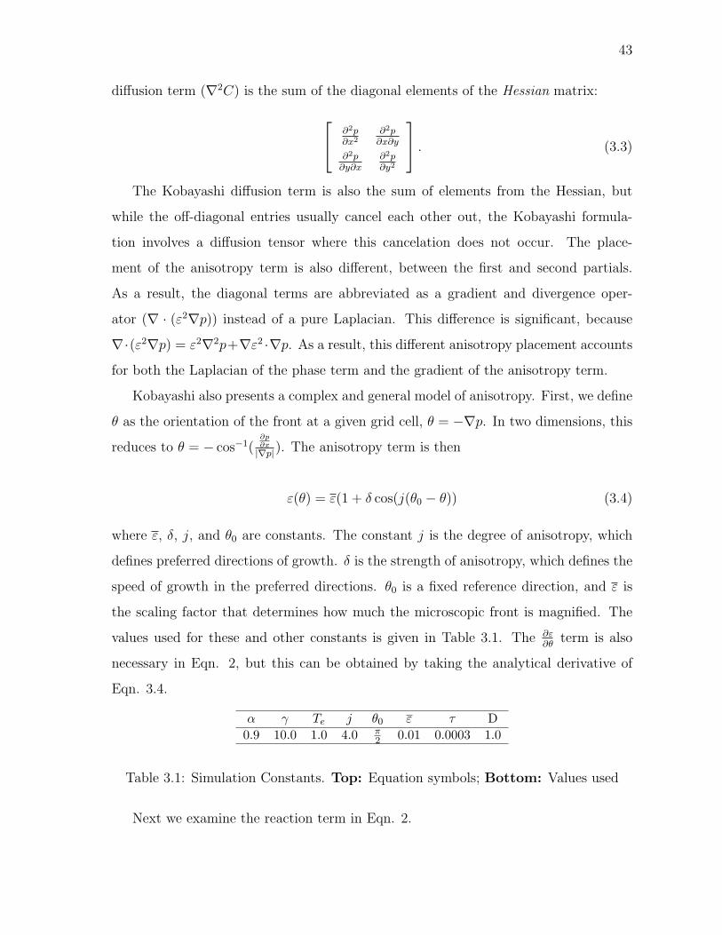
43

diffusion term (∇2C) is the sum of the diagonal elements of the Hessian matrix:

∂2p∂x2

∂2p∂x∂y

∂2p∂y∂x

∂2p∂y2

. (3.3)

The Kobayashi diffusion term is also the sum of elements from the Hessian, but

while the off-diagonal entries usually cancel each other out, the Kobayashi formula-

tion involves a diffusion tensor where this cancelation does not occur. The place-

ment of the anisotropy term is also different, between the first and second partials.

As a result, the diagonal terms are abbreviated as a gradient and divergence oper-

ator (∇ · (ε2∇p)) instead of a pure Laplacian. This difference is significant, because

∇·(ε2∇p) = ε2∇2p+∇ε2 ·∇p. As a result, this different anisotropy placement accounts

for both the Laplacian of the phase term and the gradient of the anisotropy term.

Kobayashi also presents a complex and general model of anisotropy. First, we define

θ as the orientation of the front at a given grid cell, θ = −∇p. In two dimensions, this

reduces to θ = − cos−1(∂p∂x

|∇p|). The anisotropy term is then

ε(θ) = ε(1 + δ cos(j(θ0 − θ)) (3.4)

where ε, δ, j, and θ0 are constants. The constant j is the degree of anisotropy, which

defines preferred directions of growth. δ is the strength of anisotropy, which defines the

speed of growth in the preferred directions. θ0 is a fixed reference direction, and ε is

the scaling factor that determines how much the microscopic front is magnified. The

values used for these and other constants is given in Table 3.1. The ∂ε∂θ

term is also

necessary in Eqn. 2, but this can be obtained by taking the analytical derivative of

Eqn. 3.4.

α γ Te j θ0 ε τ D0.9 10.0 1.0 4.0 π

2 0.01 0.0003 1.0

Table 3.1: Simulation Constants. Top: Equation symbols; Bottom: Values used

Next we examine the reaction term in Eqn. 2.

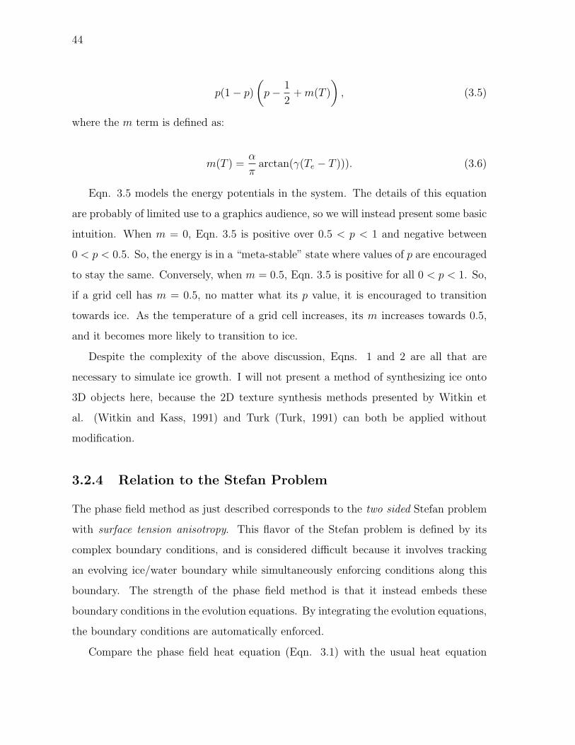
44

p(1− p)

(p− 1

2+ m(T )

), (3.5)

where the m term is defined as:

m(T ) =α

πarctan(γ(Te − T ))). (3.6)

Eqn. 3.5 models the energy potentials in the system. The details of this equation

are probably of limited use to a graphics audience, so we will instead present some basic

intuition. When m = 0, Eqn. 3.5 is positive over 0.5 < p < 1 and negative between

0 < p < 0.5. So, the energy is in a “meta-stable” state where values of p are encouraged

to stay the same. Conversely, when m = 0.5, Eqn. 3.5 is positive for all 0 < p < 1. So,

if a grid cell has m = 0.5, no matter what its p value, it is encouraged to transition

towards ice. As the temperature of a grid cell increases, its m increases towards 0.5,

and it becomes more likely to transition to ice.

Despite the complexity of the above discussion, Eqns. 1 and 2 are all that are

necessary to simulate ice growth. I will not present a method of synthesizing ice onto

3D objects here, because the 2D texture synthesis methods presented by Witkin et

al. (Witkin and Kass, 1991) and Turk (Turk, 1991) can both be applied without

modification.

3.2.4 Relation to the Stefan Problem

The phase field method as just described corresponds to the two sided Stefan problem

with surface tension anisotropy. This flavor of the Stefan problem is defined by its

complex boundary conditions, and is considered difficult because it involves tracking

an evolving ice/water boundary while simultaneously enforcing conditions along this

boundary. The strength of the phase field method is that it instead embeds these

boundary conditions in the evolution equations. By integrating the evolution equations,

the boundary conditions are automatically enforced.

Compare the phase field heat equation (Eqn. 3.1) with the usual heat equation

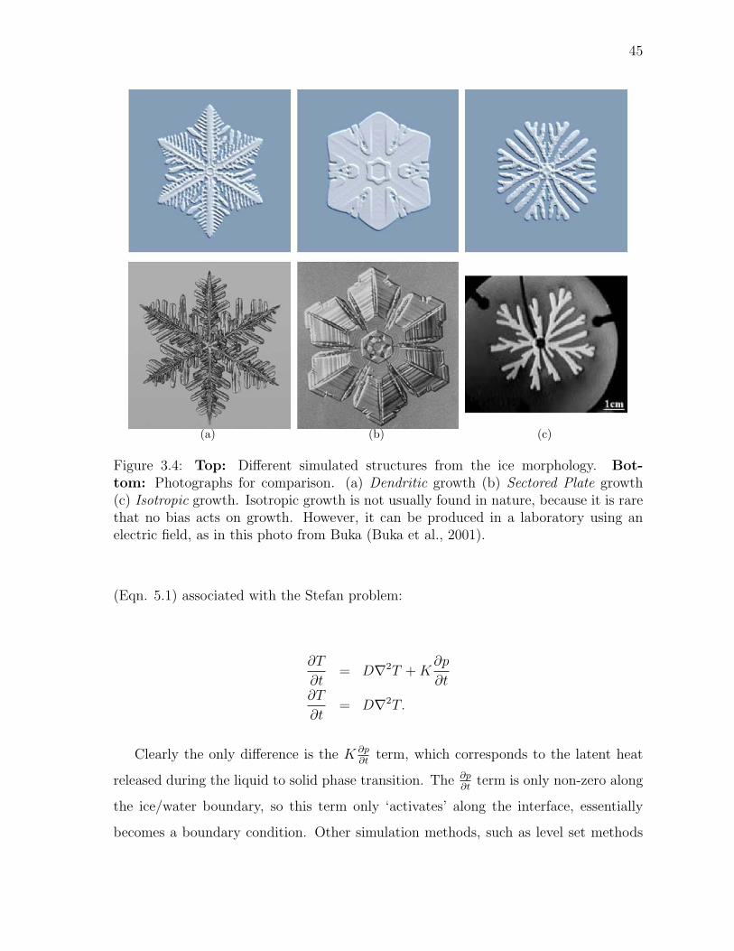
45

(a) (b) (c)

Figure 3.4: Top: Different simulated structures from the ice morphology. Bot-tom: Photographs for comparison. (a) Dendritic growth (b) Sectored Plate growth(c) Isotropic growth. Isotropic growth is not usually found in nature, because it is rarethat no bias acts on growth. However, it can be produced in a laboratory using anelectric field, as in this photo from Buka (Buka et al., 2001).

(Eqn. 5.1) associated with the Stefan problem:

∂T

∂t= D∇2T + K

∂p

∂t∂T

∂t= D∇2T.

Clearly the only difference is the K ∂p∂t

term, which corresponds to the latent heat

released during the liquid to solid phase transition. The ∂p∂t

term is only non-zero along

the ice/water boundary, so this term only ‘activates’ along the interface, essentially

becomes a boundary condition. Other simulation methods, such as level set methods

46

(Gibou et al., 2003) instead extract the location of the ice/water boundary explicitly,

compute quantities along the boundary, and then insert these quantities back into the

simulation. While there are many advantages to this approach, it is a good deal more

complex than simply Euler integrating Eqn. 3.1.

The phase evolution equation can be viewed in a similar manner. For simplicity, let

us first examine the zero surface tension case of Eqn. 3.2, where ε = 0.

τ∂p

∂t= p(1− p)

(p− 1

2+ m(T )

). (3.7)

Again, this equation is only non-zero along the boundary. The p(1− p) portion of

the cubic forces roots to occur at p = 0 and p = 1, guaranteeing that this equation is

only non-zero at in between values of p.

If we re-introduce the surface tension function ε(θ), a compact method of writing

Eqn. 3.2 is:

τ∂p

∂t= ∇ · (Φ∇p) + p(1− p)

(p− 1

2+ m(T )

), (3.8)

where Φ is the diffusion tensor:

Φ =

ε2 −ε∂ε

∂θ

ε∂ε∂θ

ε2

. (3.9)

This equation corresponds to the interface evolution of the Stefan problem (Eqn. 1.6),

∂Γ

∂t· n = D

∂T

∂ns(θ), (3.10)

where s(θ) = ε(θ)2. The correspondence is perhaps not immediately apparent, but can

be illustrated using a simpler anisotropy function, s(θ) = ε(θ)2 = 1. In this case, the

isotropic interface equation is retrieved,

∂Γ

∂t· n = D

∂T

∂n, (3.11)

47

and the phase evolution equation reduces to

τ∂p

∂t= ∇2p + p(1− p)

(p− 1

2+ m(T )

). (3.12)

The phase evolution equation is now essentially a diffusion equation, a physical process

that naturally evolves in the normal direction. Therefore, we can think of p as a smeared

out version of Γ, and view the ·n term on the left hand side of Eqn 3.11 as implicit

in the ∇2 term in Eqn. 3.12. We do not want p to smear out Γ too much however,

since it is still supposed to correspond to a sharp interface. The cubic equation on the

right hand side of Eqn. 3.12 can be thought of as a ‘sharpening’ term that prevents

the diffusion operator from smearing out the interface too badly.

This intuition remains essentially the same even if a more complex anisotropy func-

tion is used. The smeared out Γ function evolves via diffusion, and the only difference

is that the diffusion has been biased in certain preferred directions.

3.2.5 Improved Anisotropy

Eqn. 3.4 affords both simpler and richer controls for general texture synthesis than

the anisotropy term described by Witkin and Kass (Witkin and Kass, 1991). Witkin

and Kass’ formulation limits the number of preferred growth directions to 0, 2, or 4,

and all the directions must be either parallel or orthogonal. Additionally, the strength

of anisotropy in parallel directions must be the same. For example, if we prefer fast

growth along the x axis, we cannot specify different speeds for the positive and negative

directions.

Using the constant j in Eqn. 3.4, we can specify an arbitrarily high degree of

anisotropy, and with a slight modification, specify a different speed for each direction.

This is accomplished by defining a separate δi for each ith cosine lobe, and limiting the

influence of δi to the range i∗2πj≤ θ < (i+1)∗2π

j.

48

3.2.6 Possible Ice Crystal Shapes

In Fig. 4, I show the results of the simulation, starting from a point source of ice in the

center. By varying the K and δ simulation parameters, I can produce the “isotropic”,

“sectored plate”, and “dendritic” types from the ice morphology. For comparison, I

provide photos of snowflakes that illustrate these same types. Although snowflakes form

from vapor, not undercooled melts, the process of solidification is similar, and serve to

show that our results are in close agreement with naturally occurring structures.

3.2.7 Banded Optimization

A good deal of the computation in the simulation is extraneous, because in many cases

a large portion of the phase field grid is homogeneously ice or water. Eqn. 3.1 and 3.2

are only nonzero in regions where the phase field is heterogeneous, so any computation

time spent in homogeneous regions is wasted.

Some of the optimization techniques that have been proposed for phase field meth-

ods. For example, adaptive mesh refinement techniques (Provatas et al., 1999) have

been used to increase the resolution of the solution around regions of interest. Addi-

tionally diffusion Monte Carlo techniques (Plapp and Karma, 2000) have been used

to track the heat field far from the interface, resulting in significant computational

savings. Far from the interface, heat is tracked as a set of particles whose dynamics

are much cheaper to compute than fluxes over a mesh. However, these techniques also

deal with the accurate simulation of solidification at scales much smaller than the mesh

resolution. Since I am only concerned with visual simulation, these smaller scales are

not of interest.

The optimization that is of interest in the adaptive mesh and DMC methods is

the localization of computation to the grid cells along the interface. This goal can be

achieved using a simple method, similar to the “narrow band” optimization method

used for level set methods (Adalsteinsson and Sethian, 1995a). In the narrow band level

set method, instead of solving over the entire computational domain, computation is

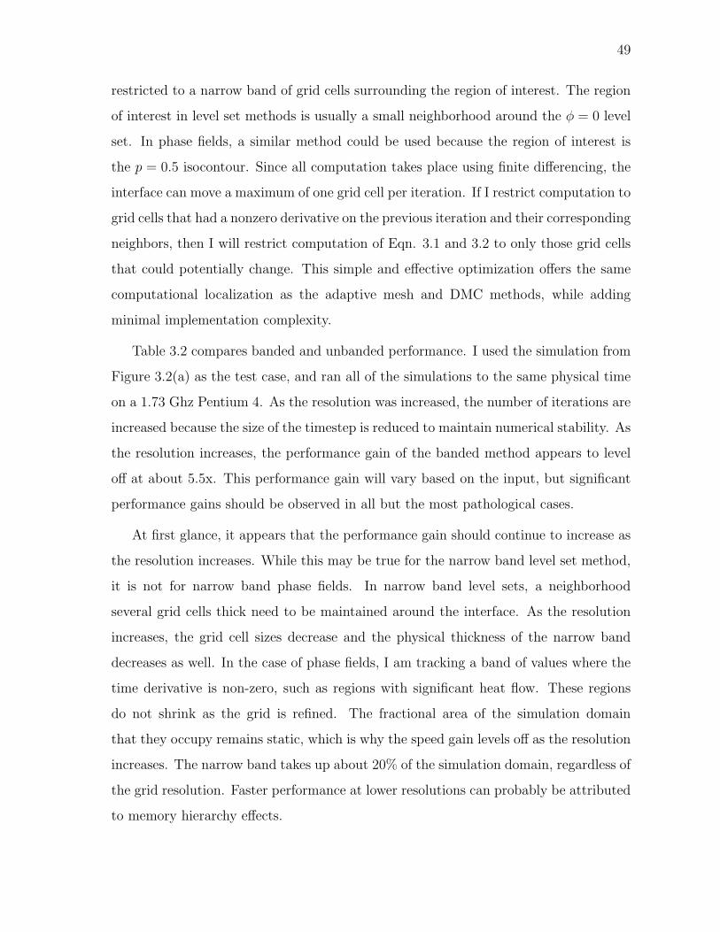
49

restricted to a narrow band of grid cells surrounding the region of interest. The region

of interest in level set methods is usually a small neighborhood around the φ = 0 level

set. In phase fields, a similar method could be used because the region of interest is

the p = 0.5 isocontour. Since all computation takes place using finite differencing, the

interface can move a maximum of one grid cell per iteration. If I restrict computation to

grid cells that had a nonzero derivative on the previous iteration and their corresponding

neighbors, then I will restrict computation of Eqn. 3.1 and 3.2 to only those grid cells

that could potentially change. This simple and effective optimization offers the same

computational localization as the adaptive mesh and DMC methods, while adding

minimal implementation complexity.

Table 3.2 compares banded and unbanded performance. I used the simulation from

Figure 3.2(a) as the test case, and ran all of the simulations to the same physical time

on a 1.73 Ghz Pentium 4. As the resolution was increased, the number of iterations are

increased because the size of the timestep is reduced to maintain numerical stability. As

the resolution increases, the performance gain of the banded method appears to level

off at about 5.5x. This performance gain will vary based on the input, but significant

performance gains should be observed in all but the most pathological cases.

At first glance, it appears that the performance gain should continue to increase as

the resolution increases. While this may be true for the narrow band level set method,

it is not for narrow band phase fields. In narrow band level sets, a neighborhood

several grid cells thick need to be maintained around the interface. As the resolution

increases, the grid cell sizes decrease and the physical thickness of the narrow band

decreases as well. In the case of phase fields, I am tracking a band of values where the

time derivative is non-zero, such as regions with significant heat flow. These regions

do not shrink as the grid is refined. The fractional area of the simulation domain

that they occupy remains static, which is why the speed gain levels off as the resolution

increases. The narrow band takes up about 20% of the simulation domain, regardless of

the grid resolution. Faster performance at lower resolutions can probably be attributed

to memory hierarchy effects.

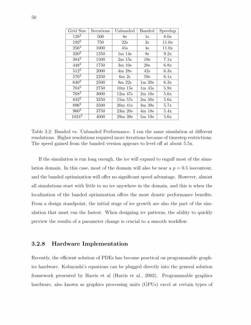
50

Grid Size Iterations Unbanded Banded Speedup1282 500 8s 1s 8.0x1922 750 22s 2s 11.0x2562 1000 45s 4s 11.0x3202 1250 1m 14s 8s 9.2x3842 1500 2m 15s 19s 7.1x4482 1750 3m 10s 28s 6.8x5122 2000 4m 28s 42s 6.3x5762 2250 6m 2s 59s 6.1x6402 2500 8m 22s 1m 20s 6.3x7042 2750 10m 15s 1m 45s 5.9x7682 3000 12m 47s 2m 16s 5.6x8322 3250 15m 57s 2m 50s 5.6x8962 3500 20m 41s 3m 39s 5.7x9602 3750 23m 20s 4m 18s 5.4x10242 4000 29m 39s 5m 19s 5.6x

Table 3.2: Banded vs. Unbanded Performance. I ran the same simulation at differentresolutions. Higher resolutions required more iterations because of timestep restrictions.The speed gained from the banded version appears to level off at about 5.5x.

If the simulation is run long enough, the ice will expand to engulf most of the simu-

lation domain. In this case, most of the domain will also be near a p = 0.5 isocontour,

and the banded optimization will offer no significant speed advantage. However, almost

all simulations start with little to no ice anywhere in the domain, and this is when the

localization of the banded optimization offers the most drastic performance benefits.

From a design standpoint, the initial stage of ice growth are also the part of the sim-

ulation that must run the fastest. When designing ice patterns, the ability to quickly

preview the results of a parameter change is crucial to a smooth workflow.

3.2.8 Hardware Implementation

Recently, the efficient solution of PDEs has become practical on programmable graph-

ics hardware. Kobayashi’s equations can be plugged directly into the general solution

framework presented by Harris et al (Harris et al., 2002). Programmable graphics

hardware, also known as graphics processing units (GPUs) excel at certain types of

51

computation, eclipsing the performance of equivalent algorithms on traditional CPUs

many times over. This performance boost stems from the fact that GPUs were designed

to exploit the SIMD (Single Instruction, Multiple Data) nature of scanline rendering.

Scanline rendering is an inherently parallel computation, since each individual pixel in

a rendered frame only depends on the scene geometry, and does not rely on the values

of neighboring pixels. Therefore, the values of multiple pixels can be computed simul-

taneously, and the same result as a serial computation is obtained. By using multiple

‘pixel pipelines’, graphics hardware exploits this parallelism and processes several pixels

in the same clock cycle. Although the clock speeds of GPUs is still currently less than

those of CPUs, this parallelism results in significantly higher performance.

While earlier generations of graphics hardware only allowed a limited set of functions

to be performed on the hardware, newer generations have allowed the use of more

general programs. Many algorithms besides scanline rendering contain an inherent

parallelism, so by mapping them to graphics hardware, large performance benefits can

be obtained. Such applications include collision detection (Govindaraju et al., 2003),

paint simulation (Baxter et al., 2004), and direct (Galoppo et al., 2005) and iterative

(Bolz et al., 2003) linear solvers.

The phase field method also maps well to graphics hardware. Since it deals mainly

with finite differences, its domain of data dependence is restricted, allowing SIMD com-

putation. Notably, solidification using the level set method does not share the same

natural mapping to GPUs, because it usually involves computing a distance field us-

ing the fast marching method (Sethian, 1999), which is an inherently serial operation.

While alternate methods of computing distance fields on the GPU do exist (Sud et al.,

2004), the fact remains that phase fields do not require any similarly special consider-

ations. Instead, phase fields can be computed using two fragment programs, which are

short enough to be listed in Appendix A.

On a high level, the GPU simulation proceeds in two stages. There are two textures,

a ‘phaseField’ texture with the p and T variables respectively packed into the red

and green channels, and an ‘eField’ texture that contains the value of ε from Eqn.

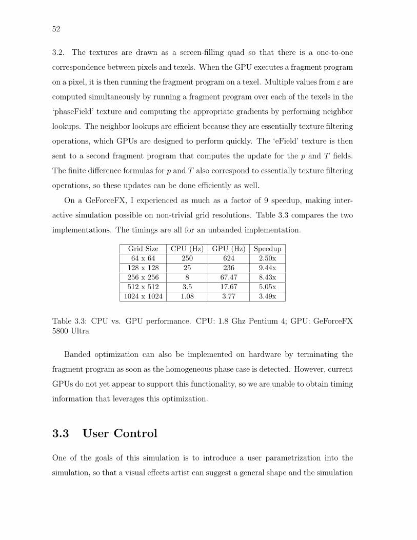
52

3.2. The textures are drawn as a screen-filling quad so that there is a one-to-one

correspondence between pixels and texels. When the GPU executes a fragment program

on a pixel, it is then running the fragment program on a texel. Multiple values from ε are

computed simultaneously by running a fragment program over each of the texels in the

‘phaseField’ texture and computing the appropriate gradients by performing neighbor

lookups. The neighbor lookups are efficient because they are essentially texture filtering

operations, which GPUs are designed to perform quickly. The ‘eField’ texture is then

sent to a second fragment program that computes the update for the p and T fields.

The finite difference formulas for p and T also correspond to essentially texture filtering

operations, so these updates can be done efficiently as well.

On a GeForceFX, I experienced as much as a factor of 9 speedup, making inter-

active simulation possible on non-trivial grid resolutions. Table 3.3 compares the two

implementations. The timings are all for an unbanded implementation.

Grid Size CPU (Hz) GPU (Hz) Speedup64 x 64 250 624 2.50x

128 x 128 25 236 9.44x256 x 256 8 67.47 8.43x512 x 512 3.5 17.67 5.05x

1024 x 1024 1.08 3.77 3.49x

Table 3.3: CPU vs. GPU performance. CPU: 1.8 Ghz Pentium 4; GPU: GeForceFX5800 Ultra

Banded optimization can also be implemented on hardware by terminating the

fragment program as soon as the homogeneous phase case is detected. However, current

GPUs do not yet appear to support this functionality, so we are unable to obtain timing

information that leverages this optimization.

3.3 User Control

One of the goals of this simulation is to introduce a user parametrization into the

simulation, so that a visual effects artist can suggest a general shape and the simulation

53

(a) (b)

(c) (d)

(e) (f)

Figure 3.5: Left to right, top to bottom: (a) The source image; (b) the seed crystaltexture; (c) simulation results after seed crystal mapping; (d) freezing temperaturemapping: White regions are the original Te value, while darker regions are lesser values;(e) the ice grown with a mapped seed crystal and freezing temperature; (f) the bumpmapped ice.

can then grow an ‘icy’ version of the shape. The phase field method supports such a

parameterization through the manipulation of its seed crystal and freezing temperature.

The seed crystal allows the user to guarantee that primary shape features are present

in the final ice, and the freezing temperature allows the user to provide further sim-

ulation hints by rating the importance of secondary features. The settings for these

parameters can be generated automatically using the methods suggested below, or in-

teractively to give the user greater control over the final result. In order to illustrate

how this works, I will grow ice in the shape of Fig. 3.5(a) as an example.

54

3.3.1 Seed Crystal Mapping

First, the user selects the most visually important features and maps them to the seed

crystal. In this case, I decided that the edges of Fig. 3.5(a) were the most important

visual feature. However, the user is free to select any arbitrary feature as the most

important.

Fig. 3.5(b) was extracted using Canny edge detection (Canny, 1986). I map these

visually important features to the seed crystal to guarantee that these features are

present in the final ice, preserving the general shape of the original image. However,

if the simulation is run on this seed crystal configuration, as shown in Fig. 3.5(c), the

desired shape is quickly lost.

The seed crystal mapping only influences the initial condition of the simulation,

so an additional parameter that influences the simulation at every timestep is also

necessary in order for the goal shape to be preserved. The freezing temperature provides

such a parameter.

3.3.2 Freezing Temperature Mapping

By varying the freezing temperature over the temperature field, we can model the

presence of impurities in the undercooled liquid. Recall that salt causes ice to melt

because it lowers the freezing temperature of the H2O, and ice then transitions back to

water if the surrounding environment is no longer cold enough to freeze it. Similarly,

if salt were present in a undercooled liquid as it was freezing, the H2O would be more

reluctant to freeze in salty regions than in regions of pure water.

If we want to promote ice growth in a specific region of the phase field, we set the

freezing temperature of that region as high as possible, to Te. If we want to suppress all

ice growth in a region, we can set the temperature of that region to zero. To rate the

importance of regions with respect to one other, we can set their freezing temperatures

between 0 and Te.

For example, in Fig. 3.5(d), white regions represent Te, while greyer regions repre-

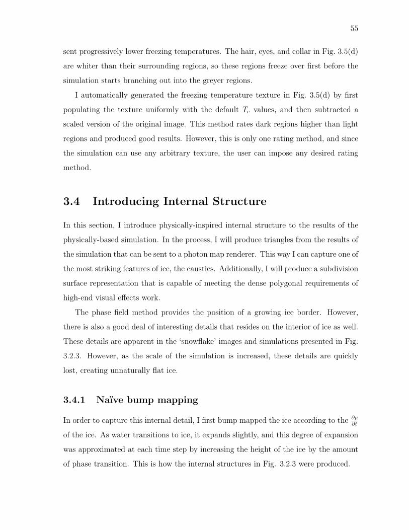
55

sent progressively lower freezing temperatures. The hair, eyes, and collar in Fig. 3.5(d)

are whiter than their surrounding regions, so these regions freeze over first before the

simulation starts branching out into the greyer regions.

I automatically generated the freezing temperature texture in Fig. 3.5(d) by first

populating the texture uniformly with the default Te values, and then subtracted a

scaled version of the original image. This method rates dark regions higher than light

regions and produced good results. However, this is only one rating method, and since

the simulation can use any arbitrary texture, the user can impose any desired rating

method.

3.4 Introducing Internal Structure

In this section, I introduce physically-inspired internal structure to the results of the

physically-based simulation. In the process, I will produce triangles from the results of

the simulation that can be sent to a photon map renderer. This way I can capture one of

the most striking features of ice, the caustics. Additionally, I will produce a subdivision

surface representation that is capable of meeting the dense polygonal requirements of

high-end visual effects work.

The phase field method provides the position of a growing ice border. However,

there is also a good deal of interesting details that resides on the interior of ice as well.

These details are apparent in the ‘snowflake’ images and simulations presented in Fig.

3.2.3. However, as the scale of the simulation is increased, these details are quickly

lost, creating unnaturally flat ice.

3.4.1 Naıve bump mapping

In order to capture this internal detail, I first bump mapped the ice according to the ∂p∂t

of the ice. As water transitions to ice, it expands slightly, and this degree of expansion

was approximated at each time step by increasing the height of the ice by the amount

of phase transition. This is how the internal structures in Fig. 3.2.3 were produced.

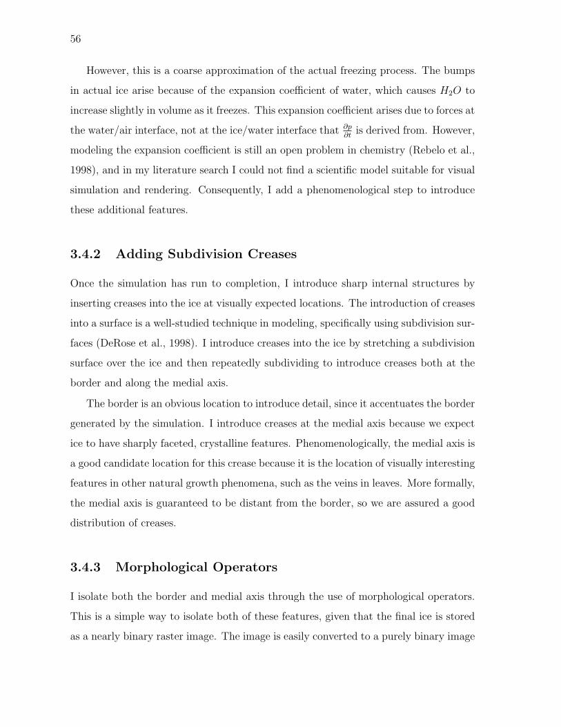
56

However, this is a coarse approximation of the actual freezing process. The bumps

in actual ice arise because of the expansion coefficient of water, which causes H2O to

increase slightly in volume as it freezes. This expansion coefficient arises due to forces at

the water/air interface, not at the ice/water interface that ∂p∂t

is derived from. However,

modeling the expansion coefficient is still an open problem in chemistry (Rebelo et al.,

1998), and in my literature search I could not find a scientific model suitable for visual

simulation and rendering. Consequently, I add a phenomenological step to introduce

these additional features.

3.4.2 Adding Subdivision Creases

Once the simulation has run to completion, I introduce sharp internal structures by

inserting creases into the ice at visually expected locations. The introduction of creases

into a surface is a well-studied technique in modeling, specifically using subdivision sur-

faces (DeRose et al., 1998). I introduce creases into the ice by stretching a subdivision

surface over the ice and then repeatedly subdividing to introduce creases both at the

border and along the medial axis.

The border is an obvious location to introduce detail, since it accentuates the border

generated by the simulation. I introduce creases at the medial axis because we expect

ice to have sharply faceted, crystalline features. Phenomenologically, the medial axis is

a good candidate location for this crease because it is the location of visually interesting

features in other natural growth phenomena, such as the veins in leaves. More formally,

the medial axis is guaranteed to be distant from the border, so we are assured a good

distribution of creases.

3.4.3 Morphological Operators

I isolate both the border and medial axis through the use of morphological operators.

This is a simple way to isolate both of these features, given that the final ice is stored

as a nearly binary raster image. The image is easily converted to a purely binary image

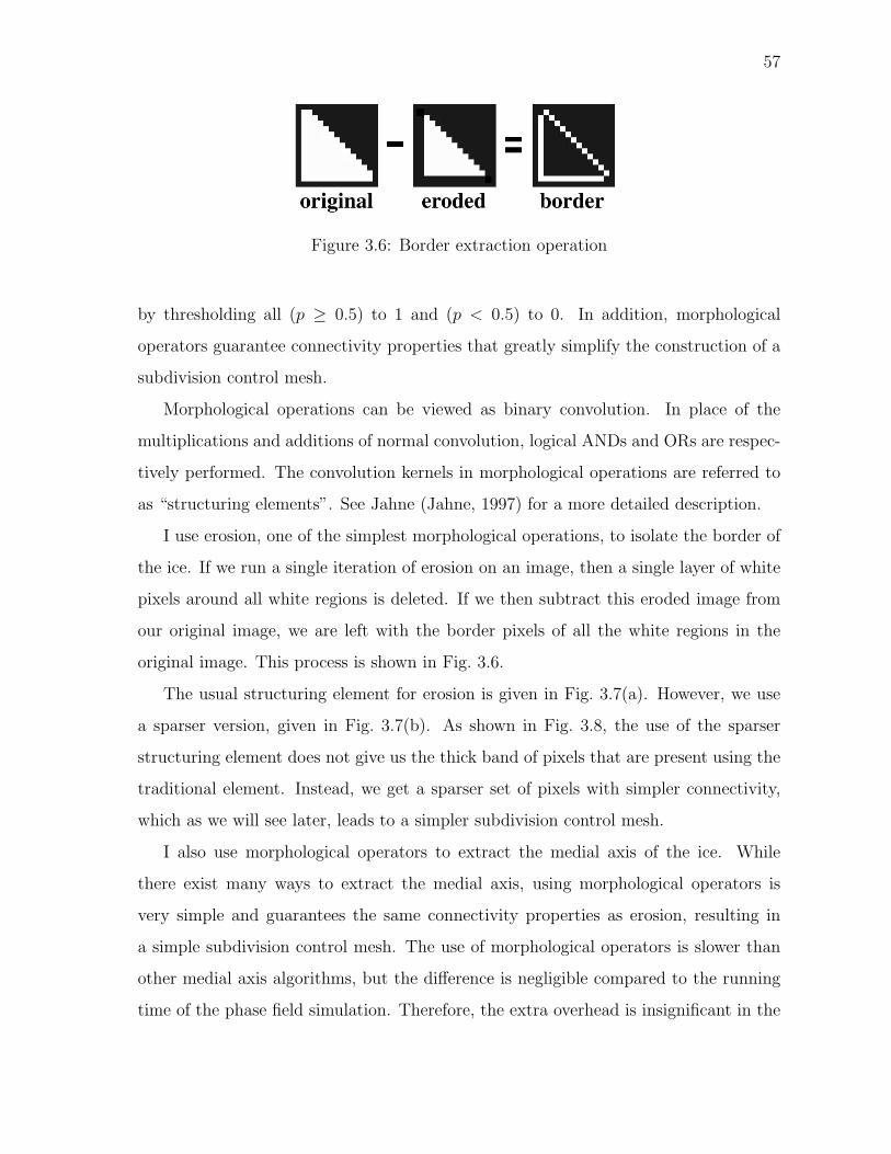
57

Figure 3.6: Border extraction operation

by thresholding all (p ≥ 0.5) to 1 and (p < 0.5) to 0. In addition, morphological

operators guarantee connectivity properties that greatly simplify the construction of a

subdivision control mesh.

Morphological operations can be viewed as binary convolution. In place of the

multiplications and additions of normal convolution, logical ANDs and ORs are respec-

tively performed. The convolution kernels in morphological operations are referred to

as “structuring elements”. See Jahne (Jahne, 1997) for a more detailed description.

I use erosion, one of the simplest morphological operations, to isolate the border of

the ice. If we run a single iteration of erosion on an image, then a single layer of white

pixels around all white regions is deleted. If we then subtract this eroded image from

our original image, we are left with the border pixels of all the white regions in the

original image. This process is shown in Fig. 3.6.

The usual structuring element for erosion is given in Fig. 3.7(a). However, we use

a sparser version, given in Fig. 3.7(b). As shown in Fig. 3.8, the use of the sparser

structuring element does not give us the thick band of pixels that are present using the

traditional element. Instead, we get a sparser set of pixels with simpler connectivity,

which as we will see later, leads to a simpler subdivision control mesh.

I also use morphological operators to extract the medial axis of the ice. While

there exist many ways to extract the medial axis, using morphological operators is

very simple and guarantees the same connectivity properties as erosion, resulting in

a simple subdivision control mesh. The use of morphological operators is slower than

other medial axis algorithms, but the difference is negligible compared to the running

time of the phase field simulation. Therefore, the extra overhead is insignificant in the

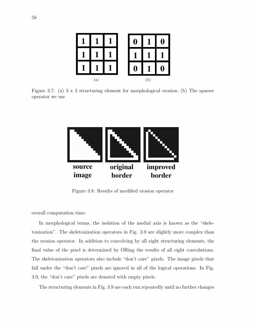
58

(a) (b)

Figure 3.7: (a) 3 x 3 structuring element for morphological erosion; (b) The sparseroperator we use

Figure 3.8: Results of modified erosion operator

overall computation time.

In morphological terms, the isolation of the medial axis is known as the “skele-

tonization”. The skeletonization operators in Fig. 3.9 are slightly more complex than

the erosion operator. In addition to convolving by all eight structuring elements, the

final value of the pixel is determined by ORing the results of all eight convolutions.

The skeletonization operators also include “don’t care” pixels. The image pixels that

fall under the “don’t care” pixels are ignored in all of the logical operations. In Fig.

3.9, the “don’t care” pixels are denoted with empty pixels.

The structuring elements in Fig. 3.9 are each run repeatedly until no further changes

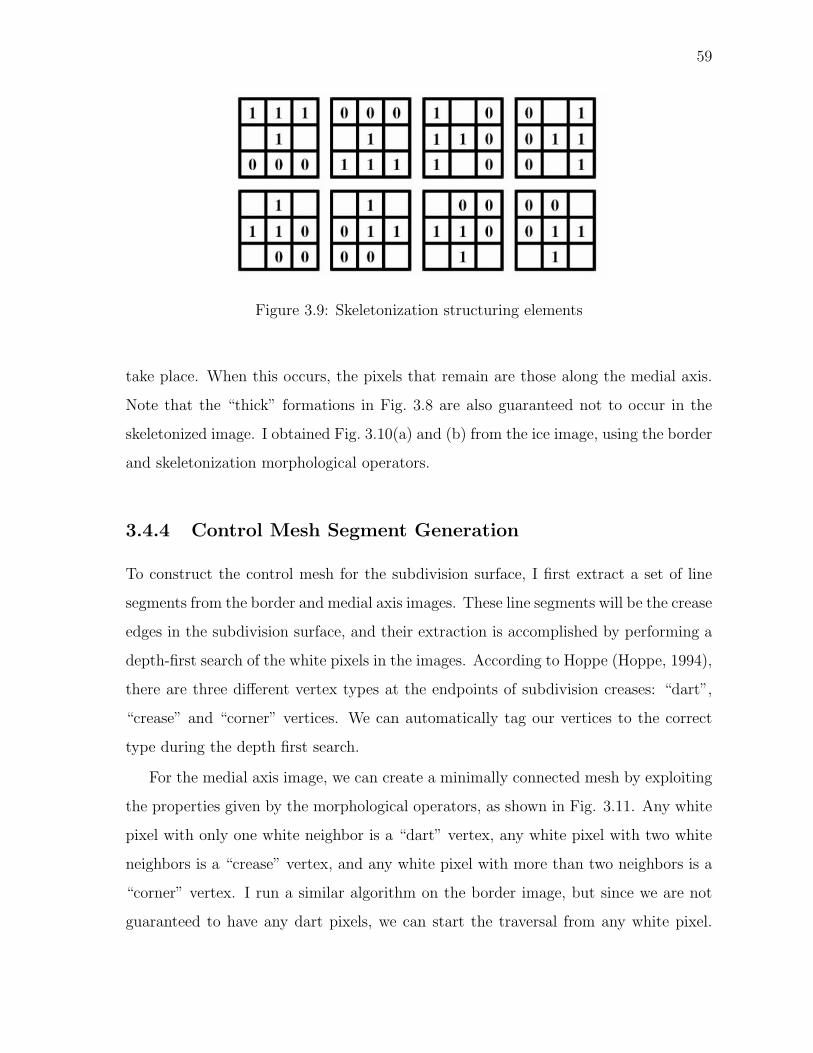
59

Figure 3.9: Skeletonization structuring elements

take place. When this occurs, the pixels that remain are those along the medial axis.

Note that the “thick” formations in Fig. 3.8 are also guaranteed not to occur in the

skeletonized image. I obtained Fig. 3.10(a) and (b) from the ice image, using the border

and skeletonization morphological operators.

3.4.4 Control Mesh Segment Generation

To construct the control mesh for the subdivision surface, I first extract a set of line

segments from the border and medial axis images. These line segments will be the crease

edges in the subdivision surface, and their extraction is accomplished by performing a

depth-first search of the white pixels in the images. According to Hoppe (Hoppe, 1994),

there are three different vertex types at the endpoints of subdivision creases: “dart”,

“crease” and “corner” vertices. We can automatically tag our vertices to the correct

type during the depth first search.

For the medial axis image, we can create a minimally connected mesh by exploiting

the properties given by the morphological operators, as shown in Fig. 3.11. Any white

pixel with only one white neighbor is a “dart” vertex, any white pixel with two white

neighbors is a “crease” vertex, and any white pixel with more than two neighbors is a

“corner” vertex. I run a similar algorithm on the border image, but since we are not

guaranteed to have any dart pixels, we can start the traversal from any white pixel.

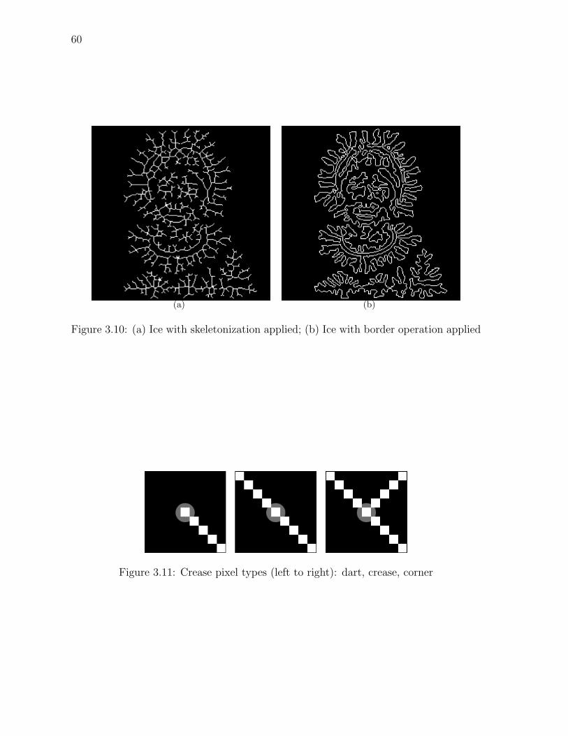
60

(a) (b)

Figure 3.10: (a) Ice with skeletonization applied; (b) Ice with border operation applied

Figure 3.11: Crease pixel types (left to right): dart, crease, corner

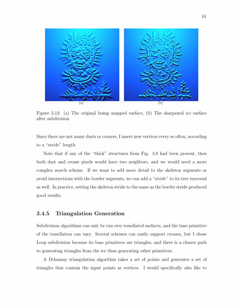
61

(a) (b)

Figure 3.12: (a) The original bump mapped surface, (b) The sharpened ice surfaceafter subdivision

Since there are not many darts or corners, I insert new vertices every so often, according

to a “stride” length.

Note that if any of the “thick” structures from Fig. 3.8 had been present, then

both dart and crease pixels would have two neighbors, and we would need a more

complex search scheme. If we want to add more detail to the skeleton segments or

avoid intersections with the border segments, we can add a “stride” to its tree traversal

as well. In practice, setting the skeleton stride to the same as the border stride produced

good results.

3.4.5 Triangulation Generation

Subdivision algorithms can only be run over tessellated surfaces, and the base primitive

of the tessellation can vary. Several schemes can easily support creases, but I chose

Loop subdivision because its base primitives are triangles, and there is a clearer path

to generating triangles from the ice than generating other primitives.

A Delaunay triangulation algorithm takes a set of points and generates a set of

triangles that contain the input points as vertices. I would specifically also like to

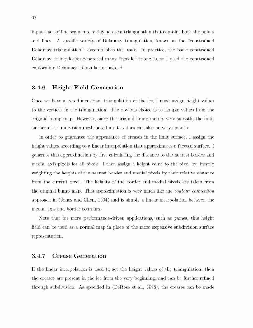
62

input a set of line segments, and generate a triangulation that contains both the points

and lines. A specific variety of Delaunay triangulation, known as the “constrained

Delaunay triangulation,” accomplishes this task. In practice, the basic constrained

Delaunay triangulation generated many “needle” triangles, so I used the constrained

conforming Delaunay triangulation instead.

3.4.6 Height Field Generation

Once we have a two dimensional triangulation of the ice, I must assign height values

to the vertices in the triangulation. The obvious choice is to sample values from the

original bump map. However, since the original bump map is very smooth, the limit

surface of a subdivision mesh based on its values can also be very smooth.

In order to guarantee the appearance of creases in the limit surface, I assign the

height values according to a linear interpolation that approximates a faceted surface. I

generate this approximation by first calculating the distance to the nearest border and

medial axis pixels for all pixels. I then assign a height value to the pixel by linearly

weighting the heights of the nearest border and medial pixels by their relative distance

from the current pixel. The heights of the border and medial pixels are taken from

the original bump map. This approximation is very much like the contour connection

approach in (Jones and Chen, 1994) and is simply a linear interpolation between the

medial axis and border contours.

Note that for more performance-driven applications, such as games, this height

field can be used as a normal map in place of the more expensive subdivision surface

representation.

3.4.7 Crease Generation

If the linear interpolation is used to set the height values of the triangulation, then

the creases are present in the ice from the very beginning, and can be further refined

through subdivision. As specified in (DeRose et al., 1998), the creases can be made

63

infinitely sharp or made arbitrarily smooth. If the mesh is already too dense for further

subdivisions, then the vertices of the triangulation can be positioned directly to the limit

surface, using the masks given in (Hoppe, 1994). The results of the crease introduction

step are shown in Fig. 3.12.

3.4.8 Rendering

Much of the interesting visual detail of ice is contained in the caustics generated by

the refracting medium. To capture this detail, I used photon mapping for rendering

(Jensen, 2001) the meshes generated by the detail reconstruction algorithm.

3.5 Implementation and Results

In this section, I give implementation details and present results generated on different

scenes using my approach.

3.5.1 Implementation

All the pipeline stages were implemented in less than 5000 lines of C++ code, excluding

the third party libraries cited below. Excluding the runtime library infrastructure, the

hardware implementation took less than 100 lines of Cg code.

For the Constrained Delaunay Triangulations, I used Jonathan Shewchuk’s Triangle

package (Shewchuk, 1996), a freely available Delaunay triangulation library that proved

to be very well documented, easy to use, and highly optimized.

For rendering, I used POV-Ray 3.5, a freely available rendering application that

supports a large shading language in addition to a nice photon map implementation.

In our banded optimization step, I found that I could not limit the band to cells

with strictly greater than zero derivatives on the previous iteration. Since I use finite

differencing to compute the derivatives, numerical noise quickly propagates through the

field, giving slightly non-zero values everywhere. Instead, I limited the band to those

64

grid cells with a previous derivative greater than 10−7.

3.5.2 Simulation Parameters

As mentioned earlier, the phase field simulation was run with the settings given in

Table 3.1. The simulation ran successfully at the resolutions up to and including 2048

x 2048.

The time step was fixed to 0.0002 at all times. At larger steps, the numerical noise

in the simulation quickly compounded. Other higher-order methods, such as Midpoint

and Runga-Kutta Four integration, were attempted as well. However, they were unable

to increase the timestep size by a factor that would have justified their cost.

3.5.3 Results

I successfully simulated ice growth in several scenes. All simulations took place on a

512 x 512 grid with the exceptions of Fig. 3.15, which was 512 x 800. The graphics

hardware implementation runs at practically interactive rates, though its performance

varies with the grid resolution.

The first scene is a pond with ice growing on a lily pad, as shown in Fig. 3.13. I ran

this simulation for 800 iterations, taking a total of 45 seconds on a GeForceFX 5800

Ultra and averaging 0.06 seconds per iterations. The constant K was set to 1.2 and δ

was set to 0.1. The scene was seeded with the veins of the lily pad, and the melting

temperature was perturbed by the grey scale intensity of the original lily pad image.

The second scene is a stained glass window, with ice growing inwards from the lead

frame. Since the lead would cool faster than the glass, this is a logical place to seed the

ice. I ran the simulation for 600 iterations, taking a total of 34 seconds on the same

GPU, taking approximately 0.06 seconds per iteration. The constant K was set to 1.2,

and δ was set to 0.04. I also inserted a small amount of random noise into the freezing

temperature map to promote non-uniform growth. Fig. 3.1 shows a detailed view on a

portion of the stained glass with ice grown on it. See Fig. 3.17, Fig. 3.16 and 3.18 for a

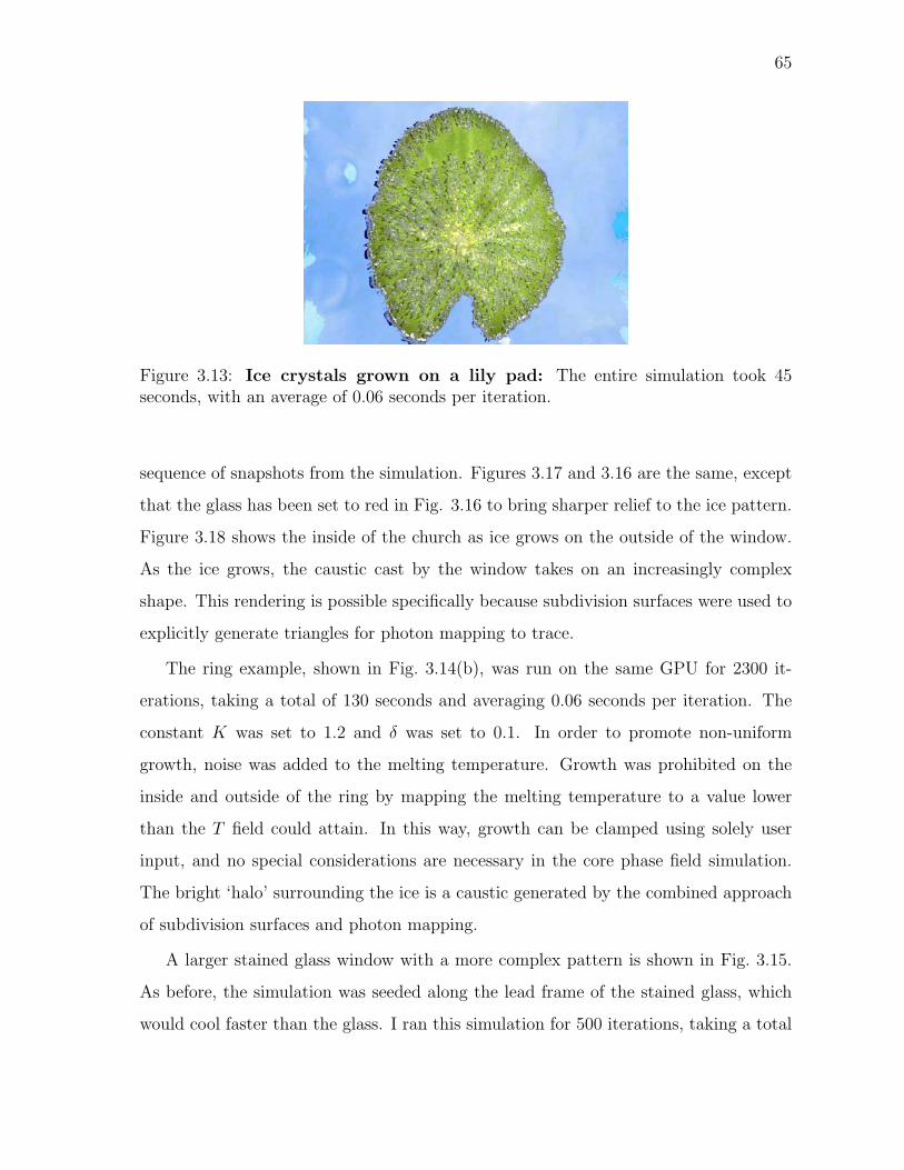
65

Figure 3.13: Ice crystals grown on a lily pad: The entire simulation took 45seconds, with an average of 0.06 seconds per iteration.

sequence of snapshots from the simulation. Figures 3.17 and 3.16 are the same, except

that the glass has been set to red in Fig. 3.16 to bring sharper relief to the ice pattern.

Figure 3.18 shows the inside of the church as ice grows on the outside of the window.

As the ice grows, the caustic cast by the window takes on an increasingly complex

shape. This rendering is possible specifically because subdivision surfaces were used to

explicitly generate triangles for photon mapping to trace.

The ring example, shown in Fig. 3.14(b), was run on the same GPU for 2300 it-

erations, taking a total of 130 seconds and averaging 0.06 seconds per iteration. The

constant K was set to 1.2 and δ was set to 0.1. In order to promote non-uniform

growth, noise was added to the melting temperature. Growth was prohibited on the

inside and outside of the ring by mapping the melting temperature to a value lower

than the T field could attain. In this way, growth can be clamped using solely user

input, and no special considerations are necessary in the core phase field simulation.

The bright ‘halo’ surrounding the ice is a caustic generated by the combined approach

of subdivision surfaces and photon mapping.

A larger stained glass window with a more complex pattern is shown in Fig. 3.15.

As before, the simulation was seeded along the lead frame of the stained glass, which

would cool faster than the glass. I ran this simulation for 500 iterations, taking a total

66

of 50 seconds on the same processor, and averaging 0.1 seconds per step. The constant

K was set to 1.2 and δ was set to 0.1.

3.5.4 Discussions and Limitations

Validating the results of the simulation is very challenging, as the simulation is very sen-

sitive to noise. In fact, it is this sensitivity that gives rise to such interesting structures.

Very specialized equipment is necessary to run any meaningful experiments, which I

unfortunately do not have access to. However, the physical validity of the phase field

methods has been proven repeatedly by researchers who have access to such equipment

in the computational physics and crystal growth communities.

The reconstruction of the lost internal detail is only physically plausible, not phys-

ically based. Further study is necessary to validate and refine this process.

The user parameterization I have presented is capable of preserving a desired shape,

but the phase field model can support additional parameters for greater user control.

The latent heat constant K, and the strength of anisotropy δ, both influence the growth

speed and the final shape of the ice, and their spatial mapping could be used to achieve

different effects. Mapping the θ0 parameter could also be used to suggest shapes, such

as ice growth in a spiral. Additional work is necessary to determine useful input ranges

for these parameters, and the effect that these settings have on performance.

With respect to rendering, I assumed homogeneous ice when in fact ice can ex-

hibit subsurface scattering, spatially variant densities, and contain pockets of air in the

form of bubbles or cracks. Some of these issues will be discussed further in chapter

5. The problem of subsurface scattering in inhomogeneous media is still an open ques-

tion in rendering however, and solving this problem fully is beyond the scope of this

dissertation.

The phase field method simulates several, but not all, forms of ice crystal growth.

The method does not extend naturally to fully 3D ice formation such as icicles, and

a fairly different approach will be necessary to capture these effects. The effect of

external forces, such as gravity, wind, and fluid flow, also have the potential to produce

67

interesting results, and these possibilities will be examined in the next chapter.

While phase fields capture a wide variety of growth types, the size of the features

that they can resolve has some strict limitations. The width of the smeared out solid

to liquid transition region is directly proportional to the value of the ε variable from

Eqn. 3.4. The underlying grid must be able fine enough to resolve features on this

length scale. Consequently, the width of the smallest dendrite tips that can be resolved

is several times larger than ε, which is already several times larger than the width of a

single grid cell.

Moreover, the surface tension anisotropy function introduces a damping force that

smears out small scale detail. This is a physical force that is independent of the simula-

tion method used. However, it is clear that in typical winter scenes, dendrite arms that

are much smaller than those prescribed by the surface tension function are common.

Therefore, other factors must be at work that introduce this additional detail. I will

describe these additional factors and suggest a method of simulating them in the next

chapter.

3.6 Summary

In Chapter 1, I hypothesized that the main visual characteristics of frost and snowflakes

are:

• Growth that can vary continuously between the dendritic and sectored plate

regimes,

• Automatic merging of nearby features that grow together,

• Optical translucency, with specularities in sharp regions.

These characteristics were addressed in this chapter using the following techniques:

• A physically-based ice growth model, the phase field method that is capable of

generating a wide variety of crystal shapes, ranging from dendritic to sectored

plate.

68

• User controls for the phase field method that allow simple and intuitive manipu-

lation of the simulation.

• A physically-inspired, novel geometric processing step that introduces internal

structure to the ice and enhances the visual realism of the final rendered image.

• A banded optimization method and a mapping to graphics hardware that enables

interactive simulation of modest-scale ice crystal growth.

In the next chapter, I will combine the phase field method with two additional

techniques: diffusion limited aggregation (DLA) and fluid solvers. The combination

of these three techniques will produce visual results that none of the techniques could

have captured alone.

69

(a) 500 timesteps (b) 1000 timesteps

(c) 1500 timesteps (d) 2000 timesteps

(e) 2500 steps

Figure 3.14: Ice crystals grown in a ring. The entire simulation took 130 seconds.

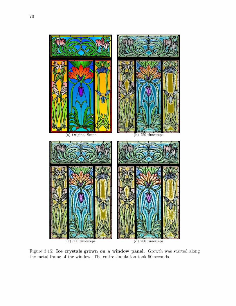
70

(a) Original Scene (b) 250 timesteps

(c) 500 timesteps (d) 750 timesteps

Figure 3.15: Ice crystals grown on a window panel. Growth was started alongthe metal frame of the window. The entire simulation took 50 seconds.

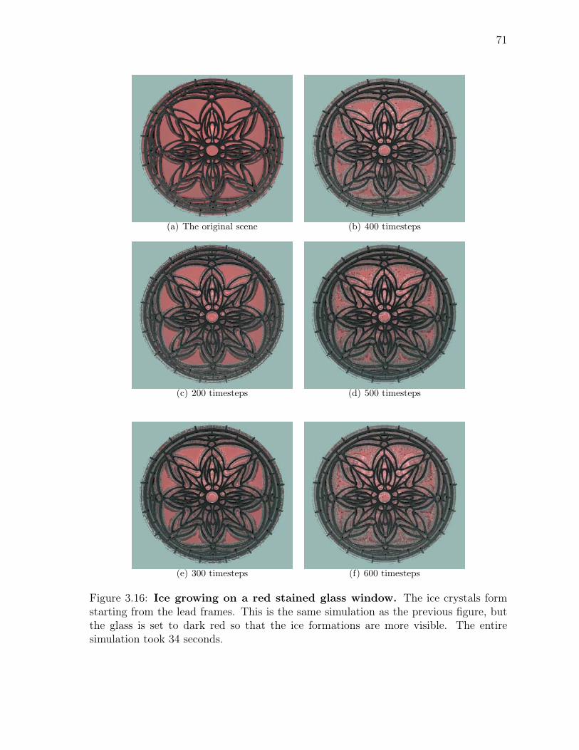
71

(a) The original scene (b) 400 timesteps

(c) 200 timesteps (d) 500 timesteps

(e) 300 timesteps (f) 600 timesteps

Figure 3.16: Ice growing on a red stained glass window. The ice crystals formstarting from the lead frames. This is the same simulation as the previous figure, butthe glass is set to dark red so that the ice formations are more visible. The entiresimulation took 34 seconds.

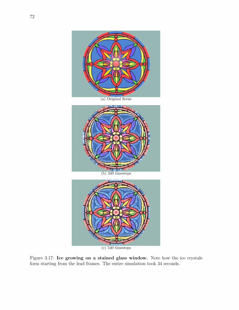
72

(a) Original Scene

(b) 340 timesteps

(c) 540 timesteps

Figure 3.17: Ice growing on a stained glass window. Note how the ice crystalsform starting from the lead frames. The entire simulation took 34 seconds.

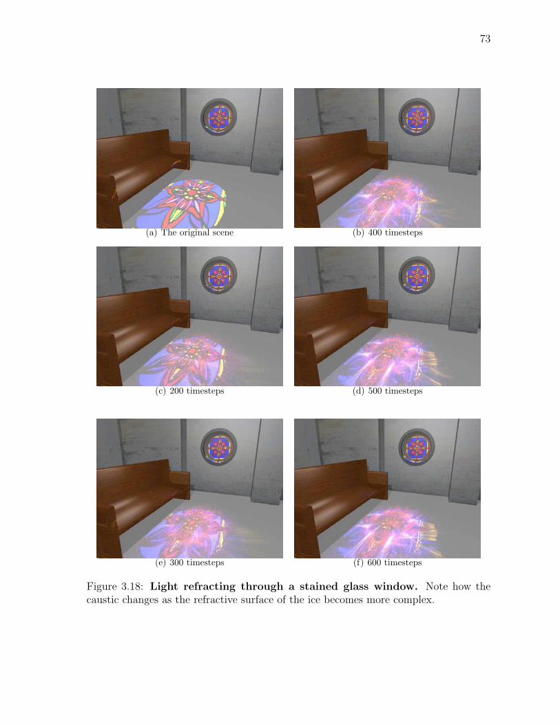
73

(a) The original scene (b) 400 timesteps

(c) 200 timesteps (d) 500 timesteps

(e) 300 timesteps (f) 600 timesteps

Figure 3.18: Light refracting through a stained glass window. Note how thecaustic changes as the refractive surface of the ice becomes more complex.

74

Chapter 4

A Hybrid Algorithm

The phase field method described in the previous chapter successfully simulates the

continuum of regimes between sectored plate and dendritic growth. However, it has

trouble handling features that are smaller than a certain threshold. This does not

appear to be an issue of merely increasing the grid resolution, because surface tension

forces inherently impose a lower limit on the width of dendrites. But, features that

are thinner than this lower threshold commonly occur in nature, so some additional

physical processes must be at work.

I hypothesize that in typical winter scenes, two simultaneous cases of the Stefan

problem are actually occurring. The first is the Stefan problem with surface tension

anisotropy from the previous chapter, and second is the zero surface tension, quasi-

steady state Stefan problem. This second problem corresponds essentially to vapor

deposition from the surrounding air. There is an algorithm known as diffusion limited

aggregation (DLA) that handles this form of the Stefan problem. I will present a

hybrid algorithm that combines phase fields and DLA, thus modeling these two growth

cases simultaneously. Since I am now modeling the air surrounding an ice crystal, I

will incorporate a flow simulation as well. The resulting growth patterns could not be

produced by any of these individual techniques alone.

The overall algorithm design is motivated by the thermodynamics of crystallization,

which is commonly broken down into three stages. Phase fields, DLA, and fluid solvers

each simulate only one stage of the crystallization process, but by combining all three

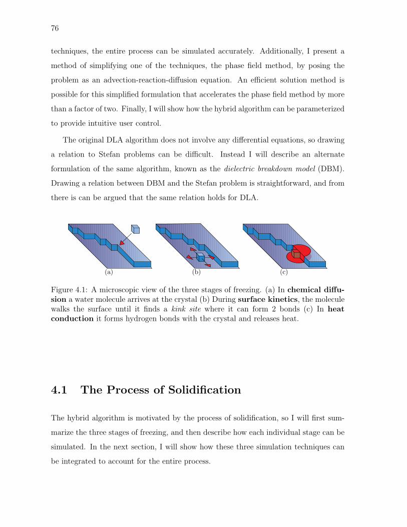
76

techniques, the entire process can be simulated accurately. Additionally, I present a

method of simplifying one of the techniques, the phase field method, by posing the

problem as an advection-reaction-diffusion equation. An efficient solution method is

possible for this simplified formulation that accelerates the phase field method by more

than a factor of two. Finally, I will show how the hybrid algorithm can be parameterized

to provide intuitive user control.

The original DLA algorithm does not involve any differential equations, so drawing

a relation to Stefan problems can be difficult. Instead I will describe an alternate

formulation of the same algorithm, known as the dielectric breakdown model (DBM).

Drawing a relation between DBM and the Stefan problem is straightforward, and from

there is can be argued that the same relation holds for DLA.

(a) (b) (c)

Figure 4.1: A microscopic view of the three stages of freezing. (a) In chemical diffu-sion a water molecule arrives at the crystal (b) During surface kinetics, the moleculewalks the surface until it finds a kink site where it can form 2 bonds (c) In heatconduction it forms hydrogen bonds with the crystal and releases heat.

4.1 The Process of Solidification

The hybrid algorithm is motivated by the process of solidification, so I will first sum-

marize the three stages of freezing, and then describe how each individual stage can be

simulated. In the next section, I will show how these three simulation techniques can

be integrated to account for the entire process.

77

4.1.1 Three Stages of Freezing

Given a free water molecule and an ice crystal, the process of solidification proceeds in

the three stages illustrated in Figure 4:

• First, the water molecule is transported to the surface of the crystal. This is

called the chemical diffusion stage.

• Second, in order for the water molecule to be considered frozen, it must form two

hydrogen bonds with the crystal. The molecule walks along the surface of the

crystal until it finds a kink site where it can form these bonds. This is called the

surface kinetics stage.

• Finally, when the molecule forms its hydrogen bonds, it releases a small amount

of heat that then diffuses through space. This is called the heat conduction stage.

If all three of these processes occur at perfectly balanced rates, then we encounter

the ideal growth case. However, ideal growth is rarely found in nature, and the process

is usually limited by the slowest of the three stages.

When the first stage is slowest, diffusion limited growth occurs. An example of this

type of growth would be a crystal surrounded by water vapor. If a water molecule

happens to collide with the crystal, then it can find a kink site and release heat.

However, these collisions are a relatively rare occurrence, so they become the limiting

factor.

When the second stage is slowest, kinetics limited growth occurs. This type of

growth can occur when a crystal is submerged in an undercooled liquid. Recall from

chemistry that an undercooled liquid is one whose temperature has slowly been low-

ered below its freezing temperature. Since the crystal is already surrounded by water

molecules, the chemical diffusion rate is no longer a factor. Instead, the limiting factor

is the speed at which water molecules can find kink sites on the surface.

When the third stage is slowest, the crystal growth literature also refers to the case

as kinetics limited growth. For clarity, we will refer to it here as heat limited growth.

78

If the crystal is surrounded by a fluid flow, then the flow of heat around the crystal is

altered. This phenomenon influences the growth of the crystal because the number of

kink sites available on a crystal surface is proportional to the magnitude of the local

heat gradient. Consequently, for sections of the crystal facing into the flow, heat is

pushed back against the crystal, creating a sharp heat gradient that promotes growth.

Conversely, for sections facing away from the flow, heat is carried away from the surface,

smearing out the gradient and suppressing growth.

For further details on the stages of solidification, the reader is referred to a compre-

hensive book by Saito (Saito, 1996).

4.1.2 Diffusion Limited Growth

The diffusion limited growth case can be modeled by diffusion limited aggregation

(DLA). The basic DLA algorithm was first described by Witten and Sander (Witten

and Sander, 1981), and is simple enough to be described informally. Given a discrete 2D

grid, a single particle representing the crystal (or ‘aggregate’) is placed in the center. A

particle called the ‘walker’ is then placed at a random location along the grid perimeter.

The particle walks randomly along adjacent grid cells until it either is adjacent to the

crystal or falls off the grid. If it is adjacent to the crystal, it sticks and becomes part

of the crystal. A new walker is then inserted at the perimeter and the random walk is

repeated. The process repeats until the aggregate achieves the size the user desires. If

we think of the aggregate as an ice crystal and the walker as a particle of water, then

the correspondence to the diffusion limited case is straightforward.

The DLA (Witten and Sander, 1981) algorithm is referred to as an ‘on-lattice’

algorithm because it takes place on a 2D grid. However, on-lattice algorithms are

susceptible to grid anisotropy artifacts. As shown in Figure 4.2(a), as the aggregate

grows larger, four distinct arms emerge. These arms have no physical justification,

and are purely an artifact of the grid representation. ‘Off-lattice’ algorithms have been

developed (Meakin, 1983) that do not suffer from this artifact, but they can be more

expensive to compute. I use on-lattice DLA because it simplifies the integration with

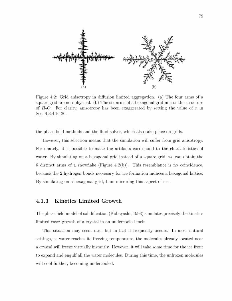
79

(a) (b)

Figure 4.2: Grid anisotropy in diffusion limited aggregation. (a) The four arms of asquare grid are non-physical. (b) The six arms of a hexagonal grid mirror the structureof H2O. For clarity, anisotropy has been exaggerated by setting the value of n inSec. 4.3.4 to 20.

the phase field methods and the fluid solver, which also take place on grids.

However, this selection means that the simulation will suffer from grid anisotropy.

Fortunately, it is possible to make the artifacts correspond to the characteristics of

water. By simulating on a hexagonal grid instead of a square grid, we can obtain the

6 distinct arms of a snowflake (Figure 4.2(b)). This resemblance is no coincidence,

because the 2 hydrogen bonds necessary for ice formation induces a hexagonal lattice.

By simulating on a hexagonal grid, I am mirroring this aspect of ice.

4.1.3 Kinetics Limited Growth

The phase field model of solidification (Kobayashi, 1993) simulates precisely the kinetics

limited case: growth of a crystal in an undercooled melt.

This situation may seem rare, but in fact it frequently occurs. In most natural

settings, as water reaches its freezing temperature, the molecules already located near

a crystal will freeze virtually instantly. However, it will take some time for the ice front

to expand and engulf all the water molecules. During this time, the unfrozen molecules

will cool further, becoming undercooled.

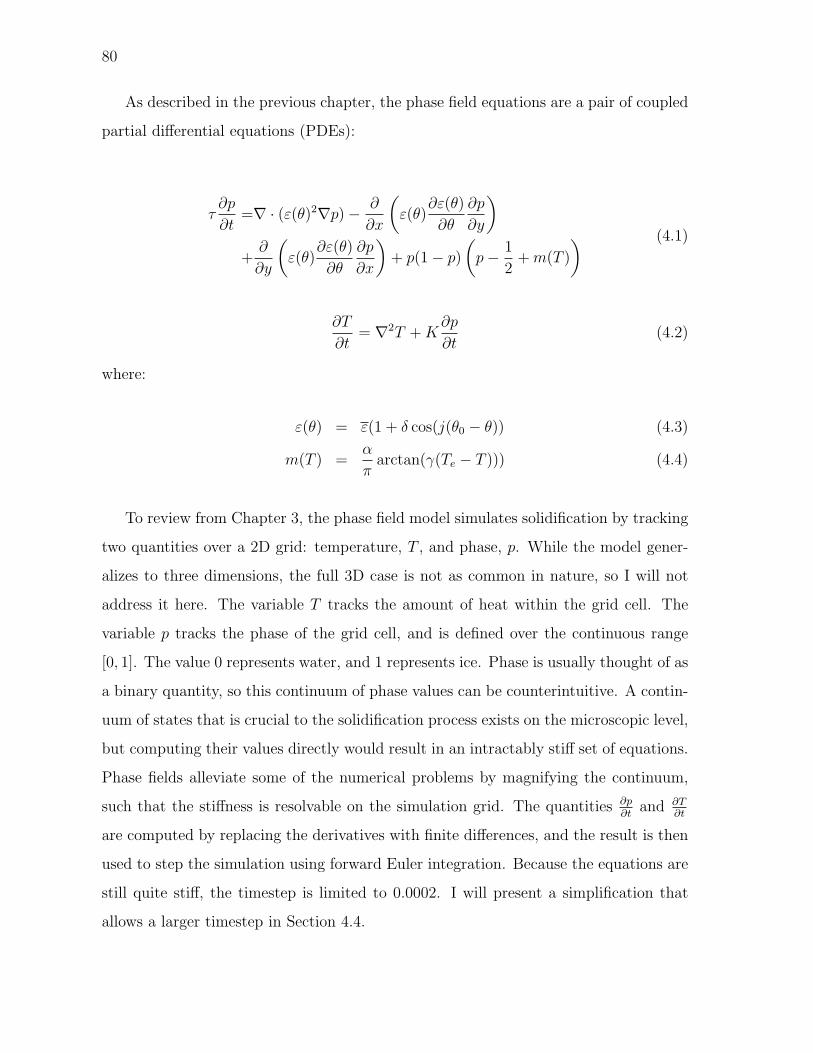
80

As described in the previous chapter, the phase field equations are a pair of coupled

partial differential equations (PDEs):

τ∂p

∂t=∇ · (ε(θ)2∇p)− ∂

∂x

(ε(θ)

∂ε(θ)

∂θ

∂p

∂y

)

+∂

∂y

(ε(θ)

∂ε(θ)

∂θ

∂p

∂x

)+ p(1− p)

(p− 1

2+ m(T )

) (4.1)

∂T

∂t= ∇2T + K

∂p

∂t(4.2)

where:

ε(θ) = ε(1 + δ cos(j(θ0 − θ)) (4.3)

m(T ) =α

πarctan(γ(Te − T ))) (4.4)

To review from Chapter 3, the phase field model simulates solidification by tracking

two quantities over a 2D grid: temperature, T , and phase, p. While the model gener-

alizes to three dimensions, the full 3D case is not as common in nature, so I will not

address it here. The variable T tracks the amount of heat within the grid cell. The

variable p tracks the phase of the grid cell, and is defined over the continuous range

[0, 1]. The value 0 represents water, and 1 represents ice. Phase is usually thought of as

a binary quantity, so this continuum of phase values can be counterintuitive. A contin-

uum of states that is crucial to the solidification process exists on the microscopic level,

but computing their values directly would result in an intractably stiff set of equations.

Phase fields alleviate some of the numerical problems by magnifying the continuum,

such that the stiffness is resolvable on the simulation grid. The quantities ∂p∂t

and ∂T∂t

are computed by replacing the derivatives with finite differences, and the result is then

used to step the simulation using forward Euler integration. Because the equations are

still quite stiff, the timestep is limited to 0.0002. I will present a simplification that

allows a larger timestep in Section 4.4.

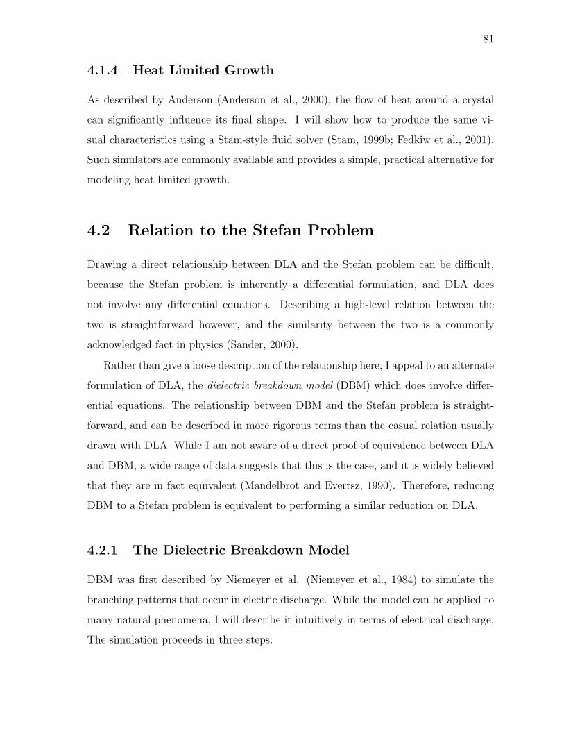
81

4.1.4 Heat Limited Growth

As described by Anderson (Anderson et al., 2000), the flow of heat around a crystal

can significantly influence its final shape. I will show how to produce the same vi-

sual characteristics using a Stam-style fluid solver (Stam, 1999b; Fedkiw et al., 2001).

Such simulators are commonly available and provides a simple, practical alternative for

modeling heat limited growth.

4.2 Relation to the Stefan Problem

Drawing a direct relationship between DLA and the Stefan problem can be difficult,

because the Stefan problem is inherently a differential formulation, and DLA does

not involve any differential equations. Describing a high-level relation between the

two is straightforward however, and the similarity between the two is a commonly

acknowledged fact in physics (Sander, 2000).

Rather than give a loose description of the relationship here, I appeal to an alternate

formulation of DLA, the dielectric breakdown model (DBM) which does involve differ-

ential equations. The relationship between DBM and the Stefan problem is straight-

forward, and can be described in more rigorous terms than the casual relation usually

drawn with DLA. While I am not aware of a direct proof of equivalence between DLA

and DBM, a wide range of data suggests that this is the case, and it is widely believed

that they are in fact equivalent (Mandelbrot and Evertsz, 1990). Therefore, reducing

DBM to a Stefan problem is equivalent to performing a similar reduction on DLA.

4.2.1 The Dielectric Breakdown Model

DBM was first described by Niemeyer et al. (Niemeyer et al., 1984) to simulate the

branching patterns that occur in electric discharge. While the model can be applied to

many natural phenomena, I will describe it intuitively in terms of electrical discharge.

The simulation proceeds in three steps:

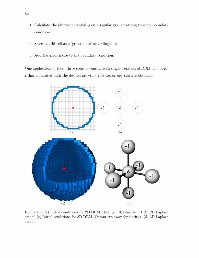
82

1. Calculate the electric potential φ on a regular grid according to some boundary

condition.

2. Select a grid cell as a ‘growth site’ according to φ.

3. Add the growth site to the boundary condition.

One application of these three steps is considered a single iteration of DBM. The algo-

rithm is iterated until the desired growth structure, or aggregate, is obtained.

(a) (b)

(c) (d)

Figure 4.3: (a) Initial conditions for 2D DBM. Red: φ = 0, Blue: φ = 1 (b) 2D Laplacestencil (c) Initial conditions for 3D DBM (Octant cut away for clarity). (d) 3D Laplacestencil

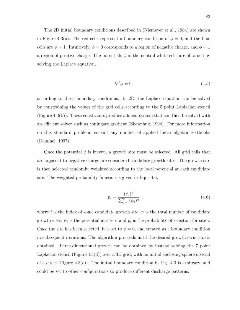
83

The 2D initial boundary conditions described in (Niemeyer et al., 1984) are shown

in Figure 4.3(a). The red cells represent a boundary condition of φ = 0, and the blue

cells are φ = 1. Intuitively, φ = 0 corresponds to a region of negative charge, and φ = 1

a region of positive charge. The potentials φ in the neutral white cells are obtained by

solving the Laplace equation,

∇2φ = 0, (4.5)

according to these boundary conditions. In 2D, the Laplace equation can be solved

by constraining the values of the grid cells according to the 5 point Laplacian stencil

(Figure 4.3(b)). These constraints produce a linear system that can then be solved with

an efficient solver such as conjugate gradient (Shewchuk, 1994). For more information

on this standard problem, consult any number of applied linear algebra textbooks

(Demmel, 1997).

Once the potential φ is known, a growth site must be selected. All grid cells that

are adjacent to negative charge are considered candidate growth sites. The growth site

is then selected randomly, weighted according to the local potential at each candidate

site. The weighted probability function is given in Eqn. 4.6,

pi =(φi)

η

∑nj=1(φj)η

(4.6)

where i is the index of some candidate growth site, n is the total number of candidate

growth sites, φi is the potential at site i, and pi is the probability of selection for site i.

Once the site has been selected, it is set to φ = 0, and treated as a boundary condition

in subsequent iterations. The algorithm proceeds until the desired growth structure is

obtained. Three-dimensional growth can be obtained by instead solving the 7 point

Laplacian stencil (Figure 4.3(d)) over a 3D grid, with an initial enclosing sphere instead

of a circle (Figure 4.3(c)). The initial boundary condition in Fig. 4.3 is arbitrary, and

could be set to other configurations to produce different discharge patterns.

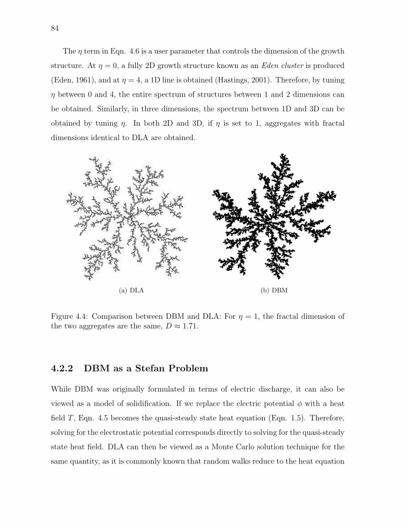
84

The η term in Eqn. 4.6 is a user parameter that controls the dimension of the growth

structure. At η = 0, a fully 2D growth structure known as an Eden cluster is produced

(Eden, 1961), and at η = 4, a 1D line is obtained (Hastings, 2001). Therefore, by tuning

η between 0 and 4, the entire spectrum of structures between 1 and 2 dimensions can

be obtained. Similarly, in three dimensions, the spectrum between 1D and 3D can be

obtained by tuning η. In both 2D and 3D, if η is set to 1, aggregates with fractal

dimensions identical to DLA are obtained.

(a) DLA (b) DBM

Figure 4.4: Comparison between DBM and DLA: For η = 1, the fractal dimension ofthe two aggregates are the same, D ≈ 1.71.

4.2.2 DBM as a Stefan Problem

While DBM was originally formulated in terms of electric discharge, it can also be

viewed as a model of solidification. If we replace the electric potential φ with a heat

field T , Eqn. 4.5 becomes the quasi-steady state heat equation (Eqn. 1.5). Therefore,

solving for the electrostatic potential corresponds directly to solving for the quasi-steady

state heat field. DLA can then be viewed as a Monte Carlo solution technique for the

same quantity, as it is commonly known that random walks reduce to the heat equation

85

(Haji-Sheikh, 1988).

This establishes the correspondence between the first equation of the Stefan prob-

lem, DBM, and by extension, DLA. The question is now how the growth site selection

step of DBM corresponds to the second equation in the Stefan problem (Eqn. 1.2):

∂Γ

∂t· n = D

∂T

∂n.

In step 2 of DBM, we select a growth site according to φ. In terms of heat, this is

equivalent to selecting a growth site according to T . This seems like a different growth

criteria than Eqn. 1.2, where the growth rate is proportional to ∂T∂n

, not T . However,

recall that the boundary of the aggregate in DBM is set to φ = 0. Let us denote

φcandidate as the potential at some candidate site, and φaggregate as the potential at its

adjacent aggregate site, and ∆x as the distance between the two sites. If we then

calculate ∂φ∂n

at the candidate site using finite differences, we obtain:

φcandidate − φaggregate

∆x=

φcandidate − 0

∆x=

φcandidate

∆x(4.7)

Since the growth site is selected proportional to φ, we can set the constant ∆x to

any arbitrary value. If we set ∆x = 1, we obtain ∂φ∂n≈ φcandidate. In other words, due

to the φ = 0 boundary condition, the potential at each candidate site is also a first

order approximation of the derivative in the normal direction. Therefore, due to the

way the boundary conditions of DBM are formulated, selecting growth sites based on

φ is equivalent to selecting sites based on ∂φ∂n

.

The growth site selection process of DBM can then be viewed as a Monte Carlo

solution method for Eqn. 1.2. Since sites with large derivatives are selected more often,

they develop faster and have greater ‘velocity’ than regions with small derivatives. This

is precisely the relation that Eqn. 1.2 describes. DLA can be thought of in an equivalent

manner, except that in this case, solving the heat equation and selecting a growth site

has been folded into the same Monte Carlo step. Statistically, more particles will walk

into regions of high heat, so these regions will receive more particles and grow with a

86

higher ‘velocity’. Again, this is precisely the relation described by Eqn. 1.2.

4.3 A Hybrid Algorithm for Ice Growth

In each of the growth types described in section 4.1, a simplifying assumption is made.

Diffusion limited growth assumes the presence of water vapor, and the absence of liquid

water and fluid flow. Kinetics limited growth assumes the presence of liquid water, and

the absence of vapor and fluid flow. Heat limited growth assumes the presence of liquid

and fluid flow, but the absence of vapor. These simplifications are apparent in the

results from each algorithm. DLA forms a branching pattern that can look more like

fungus than ice (Figure 4.11(a)), and phase field methods produce branches that look

too smooth and thick (Figure 4.11(b)). Adding fluids to either alone do not alleviate

these problems.

It seems that an environment containing all three factors (vapor, liquid, and fluid

flow) would be the most common case. If ice is forming on a window, there most likely

exists water vapor in the air, moisture on the window, and at least a small amount of

wind. To properly simulate ice growth, we should account for all of these factors.

I have developed a novel, hybrid algorithm that takes into account all three factors

by coupling the simulation techniques for each of the three growth types. I will present

the algorithm in three parts: the coupling of phase field methods and DLA, then phase

fields and fluid flow, and finally DLA and fluid flow.

4.3.1 Phase Fields and DLA

Here I choose to use DLA instead of the DBM algorithm from the previous section

because it is both more computationally tractable and provides a more natural cor-

respondence to the physical situation at hand. The random walkers from DLA map

intuitively to actual ice particles undergoing Brownian motion in the neighborhood of

the crystal. This correspondence also becomes important later when integrating DLA

with fluids. While in principle it is possible to instead apply DBM, it requires that

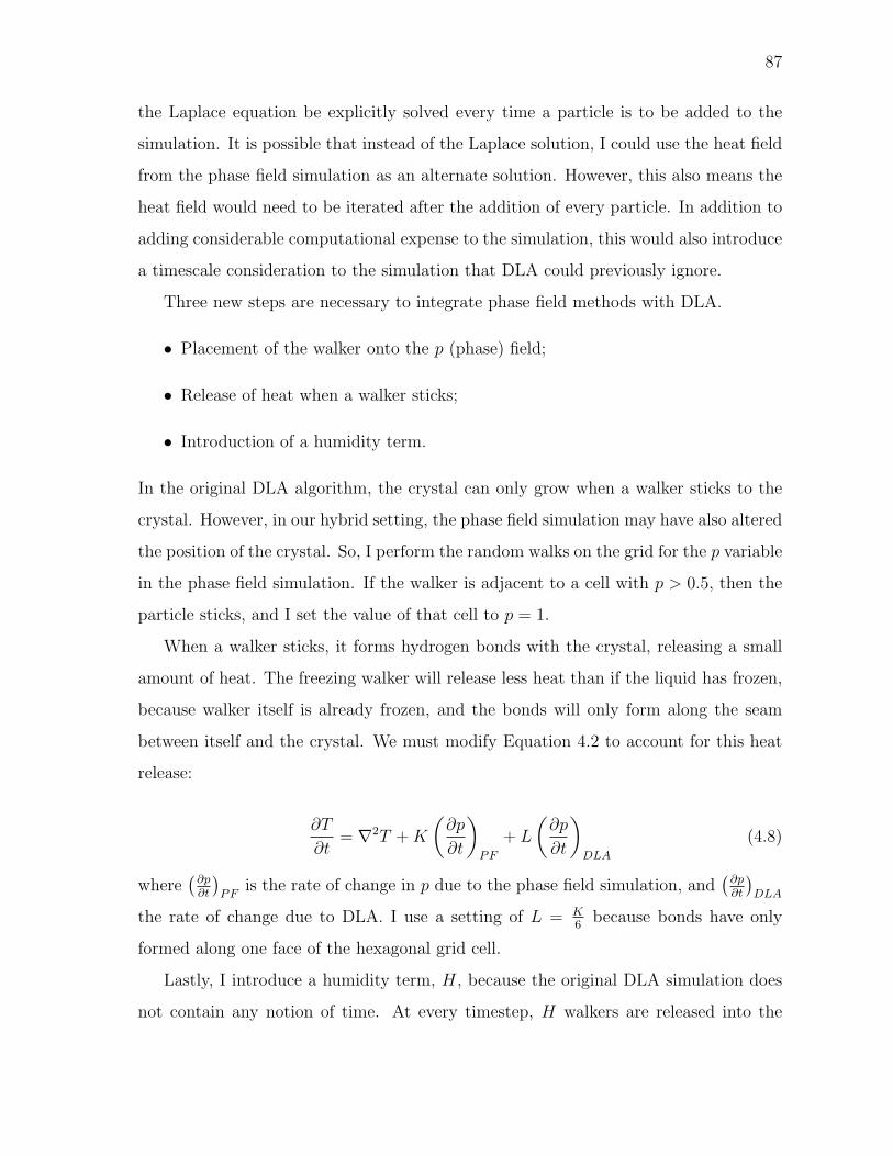
87

the Laplace equation be explicitly solved every time a particle is to be added to the

simulation. It is possible that instead of the Laplace solution, I could use the heat field

from the phase field simulation as an alternate solution. However, this also means the

heat field would need to be iterated after the addition of every particle. In addition to

adding considerable computational expense to the simulation, this would also introduce

a timescale consideration to the simulation that DLA could previously ignore.

Three new steps are necessary to integrate phase field methods with DLA.

• Placement of the walker onto the p (phase) field;

• Release of heat when a walker sticks;

• Introduction of a humidity term.

In the original DLA algorithm, the crystal can only grow when a walker sticks to the

crystal. However, in our hybrid setting, the phase field simulation may have also altered

the position of the crystal. So, I perform the random walks on the grid for the p variable

in the phase field simulation. If the walker is adjacent to a cell with p > 0.5, then the

particle sticks, and I set the value of that cell to p = 1.

When a walker sticks, it forms hydrogen bonds with the crystal, releasing a small

amount of heat. The freezing walker will release less heat than if the liquid has frozen,

because walker itself is already frozen, and the bonds will only form along the seam

between itself and the crystal. We must modify Equation 4.2 to account for this heat

release:

∂T

∂t= ∇2T + K

(∂p

∂t

)

PF

+ L

(∂p

∂t

)

DLA

(4.8)

where(

∂p∂t

)PF

is the rate of change in p due to the phase field simulation, and(

∂p∂t

)DLA

the rate of change due to DLA. I use a setting of L = K6

because bonds have only

formed along one face of the hexagonal grid cell.

Lastly, I introduce a humidity term, H, because the original DLA simulation does

not contain any notion of time. At every timestep, H walkers are released into the

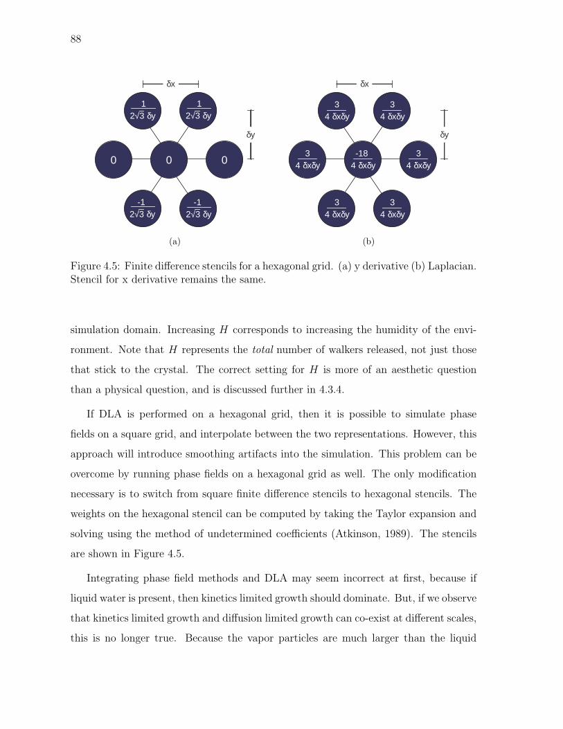
88

0 00

12√3 δy

12√3 δy

-12√3 δy

-12√3 δy

δx

δy

(a)

-184 δxδy

34 δxδy

34 δxδy

34 δxδy

34 δxδy

34 δxδy

34 δxδy

δx

δy

(b)

Figure 4.5: Finite difference stencils for a hexagonal grid. (a) y derivative (b) Laplacian.Stencil for x derivative remains the same.

simulation domain. Increasing H corresponds to increasing the humidity of the envi-

ronment. Note that H represents the total number of walkers released, not just those

that stick to the crystal. The correct setting for H is more of an aesthetic question

than a physical question, and is discussed further in 4.3.4.

If DLA is performed on a hexagonal grid, then it is possible to simulate phase

fields on a square grid, and interpolate between the two representations. However, this

approach will introduce smoothing artifacts into the simulation. This problem can be

overcome by running phase fields on a hexagonal grid as well. The only modification

necessary is to switch from square finite difference stencils to hexagonal stencils. The

weights on the hexagonal stencil can be computed by taking the Taylor expansion and

solving using the method of undetermined coefficients (Atkinson, 1989). The stencils

are shown in Figure 4.5.

Integrating phase field methods and DLA may seem incorrect at first, because if

liquid water is present, then kinetics limited growth should dominate. But, if we observe

that kinetics limited growth and diffusion limited growth can co-exist at different scales,

this is no longer true. Because the vapor particles are much larger than the liquid

89

molecules, the freezing vapor front will expand much faster than the freezing liquid

front. Once the vapor has filled the domain with branches, the liquid will take over

and freeze everything into a solid plate.

4.3.2 Phase Fields and Fluid Flow

Anderson, et al. (Anderson et al., 2000) derived a model that couples the phase field

equations and the Navier-Stokes equations. Rather than using this more complex for-

mulation, I have found the major features of solidification in a flow can be captured

by simply advecting the heat field with the “Stable Fluid” solver described in (Stam,

1999b).

Anderson, et al. (Anderson et al., 2000) does not present any simulation results

visually, so I will instead compare our results to those of Al-Rawahi and Tryggvason

(Al-Rawahi and Tryggvason, 2002). Since this paper does not use a phase field model,

exactly matching simulation parameters for comparison is difficult. But, the paper

observes the following features of growth in a flow:

• Fast growth in regions facing upstream (into flow)

• Stunted growth in regions facing downstream (away from flow)

• Asymmetric growth in regions perpendicular to the flow.

I can reproduce all of these features using the coupling of phase fields methods and a

“Stable Fluid” solver.

I treat the crystal as an internal obstacle in the fluid solver. After each pair of

phase field and DLA steps, I set any grid cell with p > 0.5 to an obstacle in the fluid

domain. I then set the velocities in the obstacle interior to zero, and along the obstacle

boundary to the no-slip condition. The velocity field u is then advanced as described

by Stam (Stam, 1999b). For a lucid description of implementing internal obstacles and

various boundary conditions, please refer to Griebel et al. (Griebel et al., 1997).

90

The resultant velocity field u can be used to advance a density field. In this case,

the density field is the temperature field T from the phase field simulation. Note that

if the fluid solver implements a diffusion constant for the density field, it must be set

to zero. Observe that the PDE for a temperature field T (Eqn. 4.2) and the PDE for

a moving density field ρ (Eqn. 4.9) both contain the diffusion operator ∇2.

∂ρ

∂t= −(u · ∇)ρ + κ∇2ρ (4.9)

If the diffusion constant κ in Eqn. 4.9 is nonzero, then the temperature field T will

incorrectly be diffused twice; once by Eqn. 4.2 and once by Eqn. 4.9. If κ is set to zero

in Eqn. 4.9, the correct result is obtained.

In the examples of (Al-Rawahi and Tryggvason, 2002), the crystals are grown from

a dot of ice in the center. The left wall is set to an inflow condition, and the other

walls are set to an outflow condition. The equivalent of the j parameter from the phase

field equations is set to 4, meaning that four axis-aligned dendrite arms are desired.

The arms are positioned so that one is growing upstream, one downstream, and two

perpendicular to the flow. The results of their simulation are shown in Figure 4.6(a),

and the three growth features mentioned earlier are clearly visible. The results of my

simulation, with similar settings, are shown in Figure 4.6(b). Although the features do

not align exactly, the method clearly produces the same growth features.

4.3.3 DLA and Fluid Flow

The integration of DLA and simplified fluid flow has been studied by the physics com-

munity in the past. In particular, Nagatani and Sagues (Nagatani and Sagues, 1991)

models the fluid as a uniform velocity field, and Toussaint et al. (Touissaint et al.,

1992) use Lattice Boltzmann-type cellular automata. However, I require no such sim-

plification. Since the DLA and phase field simulations share the p field, integrating

phase field methods and with the fluid solver automatically integrates DLA with the

full set of Navier-Stokes equations.

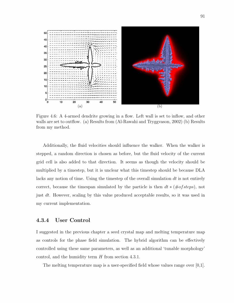
91

(a) (b)

Figure 4.6: A 4-armed dendrite growing in a flow. Left wall is set to inflow, and otherwalls are set to outflow. (a) Results from (Al-Rawahi and Tryggvason, 2002) (b) Resultsfrom my method.

Additionally, the fluid velocities should influence the walker. When the walker is

stepped, a random direction is chosen as before, but the fluid velocity of the current

grid cell is also added to that direction. It seems as though the velocity should be

multiplied by a timestep, but it is unclear what this timestep should be because DLA

lacks any notion of time. Using the timestep of the overall simulation dt is not entirely

correct, because the timespan simulated by the particle is then dt ∗ (#ofsteps), not

just dt. However, scaling by this value produced acceptable results, so it was used in

my current implementation.

4.3.4 User Control

I suggested in the previous chapter a seed crystal map and melting temperature map

as controls for the phase field simulation. The hybrid algorithm can be effectively

controlled using these same parameters, as well as an additional ‘tunable morphology’

control, and the humidity term H from section 4.3.1.

The melting temperature map is a user-specified field whose values range over [0,1].

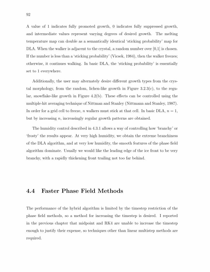
92

A value of 1 indicates fully promoted growth, 0 indicates fully suppressed growth,

and intermediate values represent varying degrees of desired growth. The melting

temperature map can double as a semantically identical ‘sticking probability’ map for

DLA. When the walker is adjacent to the crystal, a random number over [0,1] is chosen.

If the number is less than a ‘sticking probability’ (Vicsek, 1984), then the walker freezes;

otherwise, it continues walking. In basic DLA, the ‘sticking probability’ is essentially

set to 1 everywhere.

Additionally, the user may alternately desire different growth types from the crys-

tal morphology, from the random, lichen-like growth in Figure 3.2.3(c), to the regu-

lar, snowflake-like growth in Figure 4.2(b). These effects can be controlled using the

multiple-hit averaging technique of Nittman and Stanley (Nittmann and Stanley, 1987).

In order for a grid cell to freeze, n walkers must stick at that cell. In basic DLA, n = 1,

but by increasing n, increasingly regular growth patterns are obtained.

The humidity control described in 4.3.1 allows a way of controlling how ‘branchy’ or

‘frosty’ the results appear. At very high humidity, we obtain the extreme branchiness

of the DLA algorithm, and at very low humidity, the smooth features of the phase field

algorithm dominate. Usually we would like the leading edge of the ice front to be very

branchy, with a rapidly thickening front trailing not too far behind.

4.4 Faster Phase Field Methods

The performance of the hybrid algorithm is limited by the timestep restriction of the

phase field methods, so a method for increasing the timestep is desired. I reported

in the previous chapter that midpoint and RK4 are unable to increase the timestep

enough to justify their expense, so techniques other than linear multistep methods are

required.

93

(a) With diagonal terms (b) Without diagonal terms

Figure 4.7: Results of a phase field simulation with and without the diagonal termsof the diffusion tensor. While the side branching is noticeably smoother, the overallfeatures remain intact.

Recall the PDE for phase:

τ∂p

∂t= ∇ · (ε(θ)2∇p)− ∂

∂x

(ε(θ)

∂ε(θ)

∂θ

∂p

∂y

)

+∂

∂y

(ε(θ)

∂ε(θ)

∂θ

∂p

∂x

)+ p(1− p)

(p− 1

2+ m(T )

)

I first observe that the partial derivative terms can be thought of as the sum of the

entries in a variable coefficient Hessian matrix. Equations 4.1 and 4.2 resemble the

reaction-diffusion equations described in (Turk, 1991; Witkin and Kass, 1991). How-

ever, only the diagonal entries of the Hessian are used in (Witkin and Kass, 1991). To

see if such a simplification can be applied here, I ran experiments with a forward Euler

implementation, omitting the − ∂∂x

(ε∂ε

∂θ∂p∂y

)+ ∂

∂y

(ε∂ε

∂θ∂p∂x

)term. Although the results are

noticeably smoother, the branching features remained the same (Fig. 4.7). Informally

we can think of this as truncating higher order terms from the non-linear diffusion

operator.

94

A simplified phase PDE can now be written:

τ∂p

∂t= ∇ · (ε(θ)2∇p) + p(1− p)

(p− 1

2+ m(T )

)

By applying the identity ∇ · (α2∇p) = ∇α2 · ∇p + α2∇2p, this becomes:

τ∂p

∂t= ∇ε(θ)2 · ∇p + ε(θ)2∇2p + p(1− p)

(p− 1

2+ m(T )

). (4.10)

This is a non-linear advection-reaction-diffusion equation. If we now apply a second

order accurate temporal scheme, then we will be able to take larger timesteps. For

compactness of notation, I will abbreviate ε(θ)2 to α, and denote the value of p at grid

coordinate (i, j) and timestep n as pni,j.

4.4.1 Second Order Accuracy In Time

The Lax-Wendroff scheme is applied to the advection term ∇ε(θ)2 · ∇p. In the x

direction, I replace the old scheme:

∂α

∂x

∂p

∂x≈ αi−1,j − αi+1,j

∆x

pni−1,j − pn

i+1,j

∆x

with the Lax-Wendroff scheme:

∂α

∂x

∂p

∂x≈αi−1,j − αi+1,j

∆x

pni−1,j − pn

i+1,j

∆x−

(αi−1,j − αi+1,j

∆x

)2 pni−1,j − 2pn

i,j + pni+1,j

(∆x)2

The equivalent scheme in the y direction is:

∂α

∂y

∂p

∂y≈αi,j−1 − αi,j+1

∆y

pni,j−1 − pn

i,j1

∆y−

(αi,j−1 − αi,j+1

∆y

)2 pni,j−1 − 2pn

i,j + pni,j+1

(∆y)2.

Next, the Crank-Nicolson discretization is applied to the diffusion term, ε(θ)2∇2p.

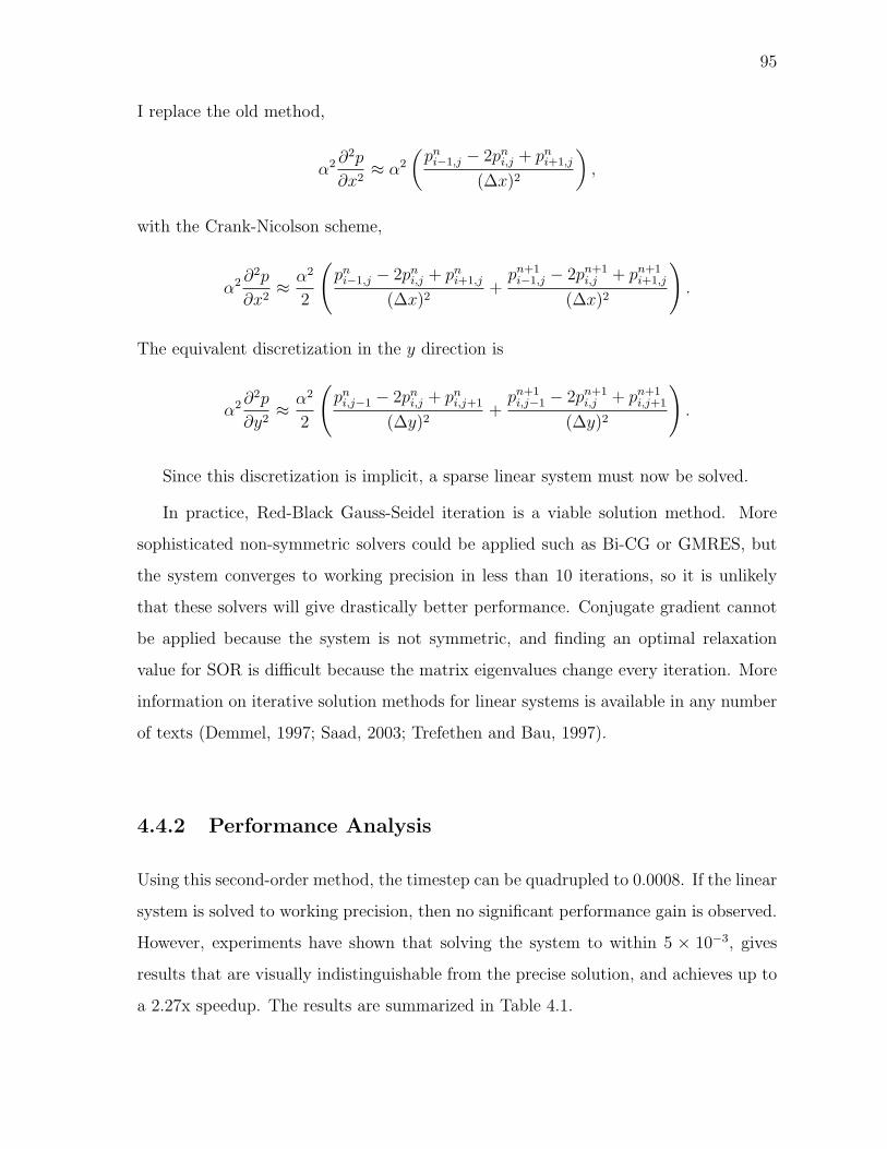
95

I replace the old method,

α2 ∂2p

∂x2≈ α2

(pn

i−1,j − 2pni,j + pn

i+1,j

(∆x)2

),

with the Crank-Nicolson scheme,

α2 ∂2p

∂x2≈ α2

2

(pn

i−1,j − 2pni,j + pn

i+1,j

(∆x)2+

pn+1i−1,j − 2pn+1

i,j + pn+1i+1,j

(∆x)2

).

The equivalent discretization in the y direction is

α2 ∂2p

∂y2≈ α2

2

(pn

i,j−1 − 2pni,j + pn

i,j+1

(∆y)2+

pn+1i,j−1 − 2pn+1

i,j + pn+1i,j+1

(∆y)2

).

Since this discretization is implicit, a sparse linear system must now be solved.

In practice, Red-Black Gauss-Seidel iteration is a viable solution method. More

sophisticated non-symmetric solvers could be applied such as Bi-CG or GMRES, but

the system converges to working precision in less than 10 iterations, so it is unlikely

that these solvers will give drastically better performance. Conjugate gradient cannot

be applied because the system is not symmetric, and finding an optimal relaxation

value for SOR is difficult because the matrix eigenvalues change every iteration. More

information on iterative solution methods for linear systems is available in any number

of texts (Demmel, 1997; Saad, 2003; Trefethen and Bau, 1997).

4.4.2 Performance Analysis

Using this second-order method, the timestep can be quadrupled to 0.0008. If the linear

system is solved to working precision, then no significant performance gain is observed.

However, experiments have shown that solving the system to within 5 × 10−3, gives

results that are visually indistinguishable from the precise solution, and achieves up to

a 2.27x speedup. The results are summarized in Table 4.1.

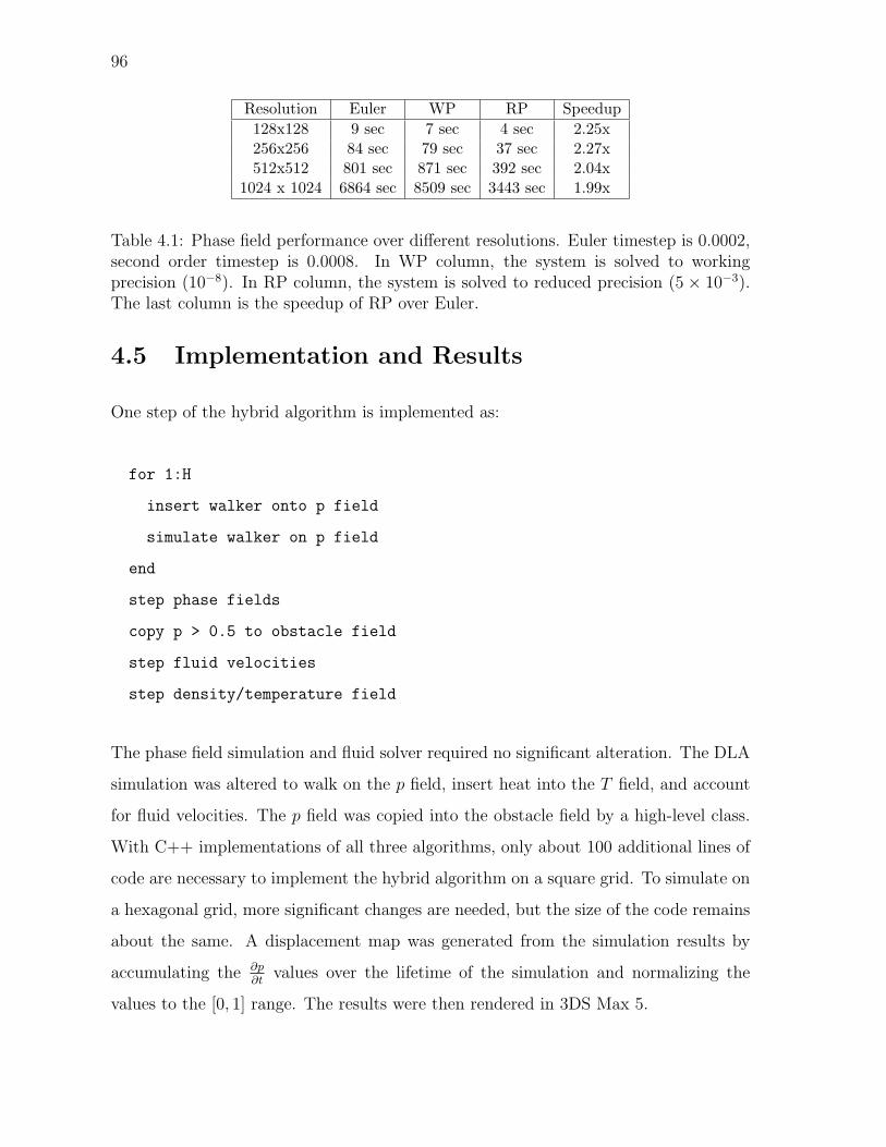
96

Resolution Euler WP RP Speedup128x128 9 sec 7 sec 4 sec 2.25x256x256 84 sec 79 sec 37 sec 2.27x512x512 801 sec 871 sec 392 sec 2.04x

1024 x 1024 6864 sec 8509 sec 3443 sec 1.99x

Table 4.1: Phase field performance over different resolutions. Euler timestep is 0.0002,second order timestep is 0.0008. In WP column, the system is solved to workingprecision (10−8). In RP column, the system is solved to reduced precision (5 × 10−3).The last column is the speedup of RP over Euler.

4.5 Implementation and Results

One step of the hybrid algorithm is implemented as:

for 1:H

insert walker onto p field

simulate walker on p field

end

step phase fields

copy p > 0.5 to obstacle field

step fluid velocities

step density/temperature field

The phase field simulation and fluid solver required no significant alteration. The DLA

simulation was altered to walk on the p field, insert heat into the T field, and account

for fluid velocities. The p field was copied into the obstacle field by a high-level class.

With C++ implementations of all three algorithms, only about 100 additional lines of

code are necessary to implement the hybrid algorithm on a square grid. To simulate on

a hexagonal grid, more significant changes are needed, but the size of the code remains

about the same. A displacement map was generated from the simulation results by

accumulating the ∂p∂t

values over the lifetime of the simulation and normalizing the

values to the [0, 1] range. The results were then rendered in 3DS Max 5.

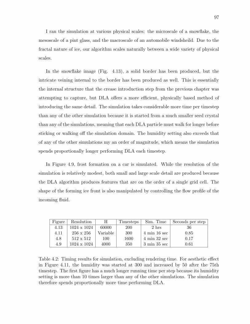
97

I ran the simulation at various physical scales: the microscale of a snowflake, the

mesoscale of a pint glass, and the macroscale of an automobile windsheild. Due to the

fractal nature of ice, our algorithm scales naturally between a wide variety of physical

scales.

In the snowflake image (Fig. 4.13), a solid border has been produced, but the

intricate veining internal to the border has been produced as well. This is essentially

the internal structure that the crease introduction step from the previous chapter was

attempting to capture, but DLA offers a more efficient, physically based method of

introducing the same detail. The simulation takes considerable more time per timestep

than any of the other simulation because it is started from a much smaller seed crystal

than any of the simulations, meaning that each DLA particle must walk for longer before

sticking or walking off the simulation domain. The humidity setting also exceeds that

of any of the other simulations my an order of magnitude, which means the simulation

spends proportionally longer performing DLA each timestep.

In Figure 4.9, frost formation on a car is simulated. While the resolution of the

simulation is relatively modest, both small and large scale detail are produced because

the DLA algorithm produces features that are on the order of a single grid cell. The

shape of the forming ice front is also manipulated by controlling the flow profile of the

incoming fluid.

Figure Resolution H Timesteps Sim. Time Seconds per step4.13 1024 x 1024 60000 200 2 hrs 364.11 256 x 256 Variable 300 4 min 16 sec 0.854.8 512 x 512 100 1600 4 min 32 sec 0.174.9 1024 x 1024 4000 350 3 min 35 sec 0.61

Table 4.2: Timing results for simulation, excluding rendering time. For aesthetic effectin Figure 4.11, the humidity was started at 300 and increased by 50 after the 75thtimestep. The first figure has a much longer running time per step because its humiditysetting is more than 10 times larger than any of the other simulations. The simulationtherefore spends proportionally more time performing DLA.

98

Figure 3.17 shows frost formation on a chilled glass. In this case, the fingering effect

on the fringe of the solidification front is reproduced faithfully. Far from the front, the

ice formed into a solid plate, but due to the non-uniform growth history, the plate is not

entirely flat. Instead the bumpy surface of the ice reflects the surrounding environment

map, producing a variety of colorful specular effects that increase the realism of the

final image.

All of the simulations were run on a 2.66 GHz Xeon processor, with timing results

(excluding rendering time) shown in Table 4.2. In Figure 4.11, the inflow fluid velocity

along the top edge was set equal to 0 along the left wall and increased quadratically

to 3.5 approaching the right wall. In Figure 4.9, the top edge was set to a parabolic

inflow of 3.5 in the center and 0 at the ends. The same simulation was used for the

hood, side panel, and windshield. For all simulations, δx, δy were set to 364

to keep the

timestep fixed.

4.6 Discussions and Limitations

In Figures 4.9-4.13, I show images of simulated ice forming in a snowflake pattern, on

a frozen window pane, on a chilled glass, and on a car in a wintery scene. For two

of these, the snowflake and chilled glass, I also present photographs for comparison.

Validating results of any simulation can be very challenging, and I found this task

especially difficult for the window and car scenes, as outdoor environments contains a

plethora of factors that can affect the growth of ice pattern in a significant way.

For Figure 4.13, the snowflake scene, the inset photograph shows that the over-

all shape and distribution of arms has been reproduced. Most notably, the intricate

network of veins internal to the border of the snowflake have been produced. DLA

alone can produce the same veins, but cannot produce the thickened border. Phase

fields from the previous chapter can produce the thick border, but cannot produce the

veins without significant intervention. The hybrid algorithm produces these features

automatically.

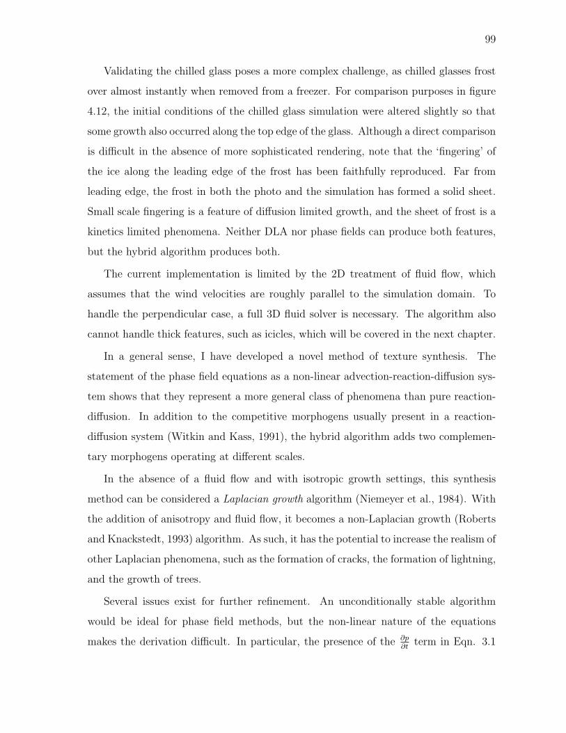
99

Validating the chilled glass poses a more complex challenge, as chilled glasses frost

over almost instantly when removed from a freezer. For comparison purposes in figure

4.12, the initial conditions of the chilled glass simulation were altered slightly so that

some growth also occurred along the top edge of the glass. Although a direct comparison

is difficult in the absence of more sophisticated rendering, note that the ‘fingering’ of

the ice along the leading edge of the frost has been faithfully reproduced. Far from

leading edge, the frost in both the photo and the simulation has formed a solid sheet.

Small scale fingering is a feature of diffusion limited growth, and the sheet of frost is a

kinetics limited phenomena. Neither DLA nor phase fields can produce both features,

but the hybrid algorithm produces both.

The current implementation is limited by the 2D treatment of fluid flow, which

assumes that the wind velocities are roughly parallel to the simulation domain. To

handle the perpendicular case, a full 3D fluid solver is necessary. The algorithm also

cannot handle thick features, such as icicles, which will be covered in the next chapter.

In a general sense, I have developed a novel method of texture synthesis. The

statement of the phase field equations as a non-linear advection-reaction-diffusion sys-

tem shows that they represent a more general class of phenomena than pure reaction-

diffusion. In addition to the competitive morphogens usually present in a reaction-

diffusion system (Witkin and Kass, 1991), the hybrid algorithm adds two complemen-

tary morphogens operating at different scales.

In the absence of a fluid flow and with isotropic growth settings, this synthesis

method can be considered a Laplacian growth algorithm (Niemeyer et al., 1984). With

the addition of anisotropy and fluid flow, it becomes a non-Laplacian growth (Roberts

and Knackstedt, 1993) algorithm. As such, it has the potential to increase the realism of

other Laplacian phenomena, such as the formation of cracks, the formation of lightning,

and the growth of trees.

Several issues exist for further refinement. An unconditionally stable algorithm

would be ideal for phase field methods, but the non-linear nature of the equations

makes the derivation difficult. In particular, the presence of the ∂p∂t

term in Eqn. 3.1

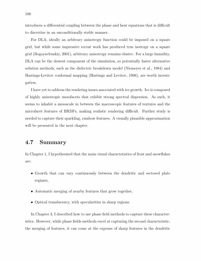
100

introduces a differential coupling between the phase and heat equations that is difficult

to discretize in an unconditionally stable manner.

For DLA, ideally an arbitrary anisotropy function could be imposed on a square

grid, but while some impressive recent work has produced true isotropy on a square

grid (Bogoyavlenskiy, 2001), arbitrary anisotropy remains elusive. For a large humidity,

DLA can be the slowest component of the simulation, so potentially faster alternative

solution methods, such as the dielectric breakdown model (Niemeyer et al., 1984) and

Hastings-Levitov conformal mapping (Hastings and Levitov, 1998), are worth investi-

gation.

I have yet to address the rendering issues associated with ice growth. Ice is composed

of highly anisotropic mesofacets that exhibit strong spectral dispersion. As such, it

seems to inhabit a mesoscale in between the macroscopic features of textures and the

microfacet features of BRDFs, making realistic rendering difficult. Further study is

needed to capture their sparkling, rainbow features. A visually plausible approximation

will be presented in the next chapter.

4.7 Summary

In Chapter 1, I hypothesized that the main visual characteristics of frost and snowflakes

are:

• Growth that can vary continuously between the dendritic and sectored plate

regimes,

• Automatic merging of nearby features that grow together,

• Optical translucency, with specularities in sharp regions.

In Chapter 3, I described how to use phase field methods to capture these character-

istics. However, while phase fields methods excel at capturing the second characteristic,

the merging of features, it can come at the expense of sharp features in the dendritic

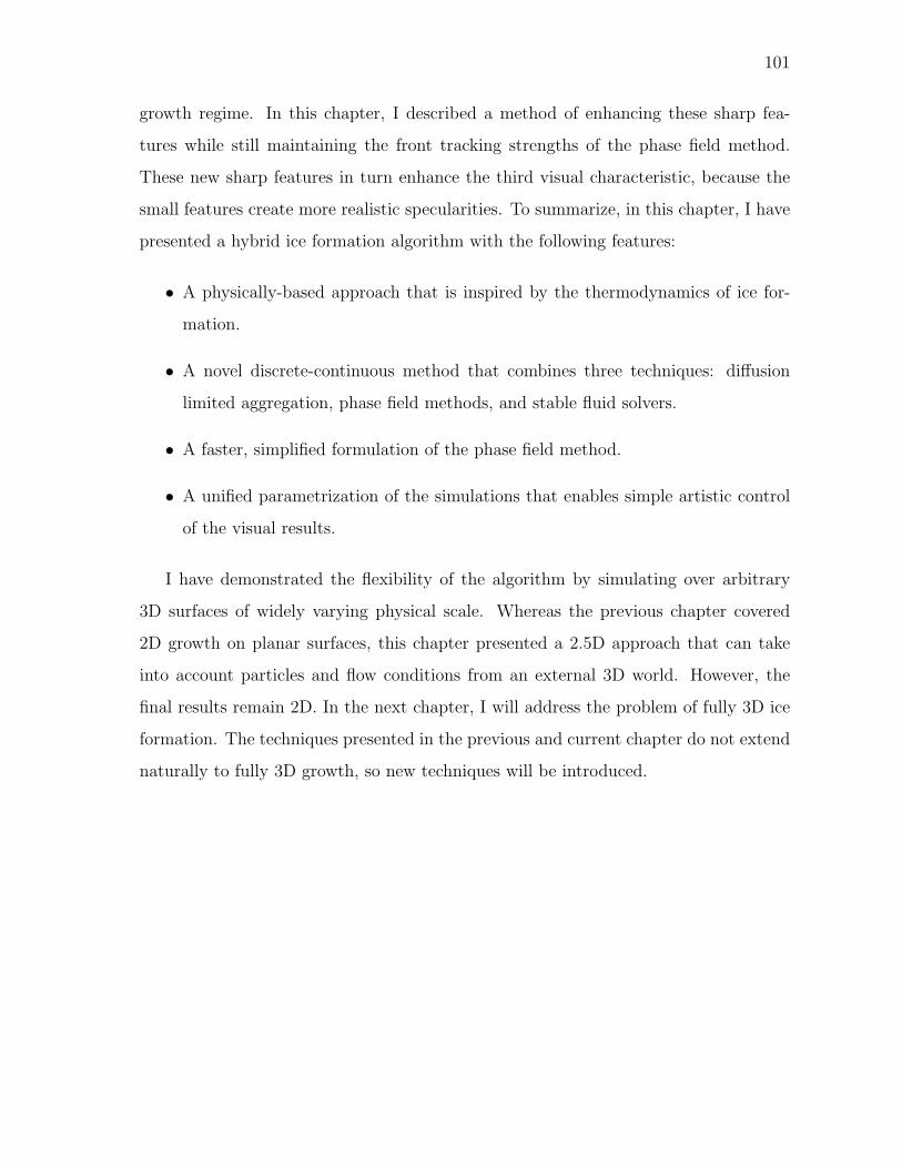
101

growth regime. In this chapter, I described a method of enhancing these sharp fea-

tures while still maintaining the front tracking strengths of the phase field method.

These new sharp features in turn enhance the third visual characteristic, because the

small features create more realistic specularities. To summarize, in this chapter, I have

presented a hybrid ice formation algorithm with the following features:

• A physically-based approach that is inspired by the thermodynamics of ice for-

mation.

• A novel discrete-continuous method that combines three techniques: diffusion

limited aggregation, phase field methods, and stable fluid solvers.

• A faster, simplified formulation of the phase field method.

• A unified parametrization of the simulations that enables simple artistic control

of the visual results.

I have demonstrated the flexibility of the algorithm by simulating over arbitrary

3D surfaces of widely varying physical scale. Whereas the previous chapter covered

2D growth on planar surfaces, this chapter presented a 2.5D approach that can take

into account particles and flow conditions from an external 3D world. However, the

final results remain 2D. In the next chapter, I will address the problem of fully 3D ice

formation. The techniques presented in the previous and current chapter do not extend

naturally to fully 3D growth, so new techniques will be introduced.

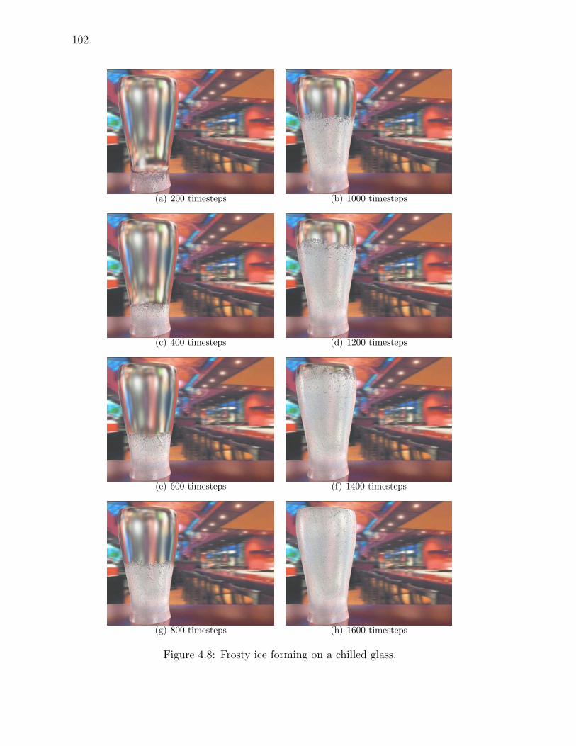
102

(a) 200 timesteps (b) 1000 timesteps

(c) 400 timesteps (d) 1200 timesteps

(e) 600 timesteps (f) 1400 timesteps

(g) 800 timesteps (h) 1600 timesteps

Figure 4.8: Frosty ice forming on a chilled glass.

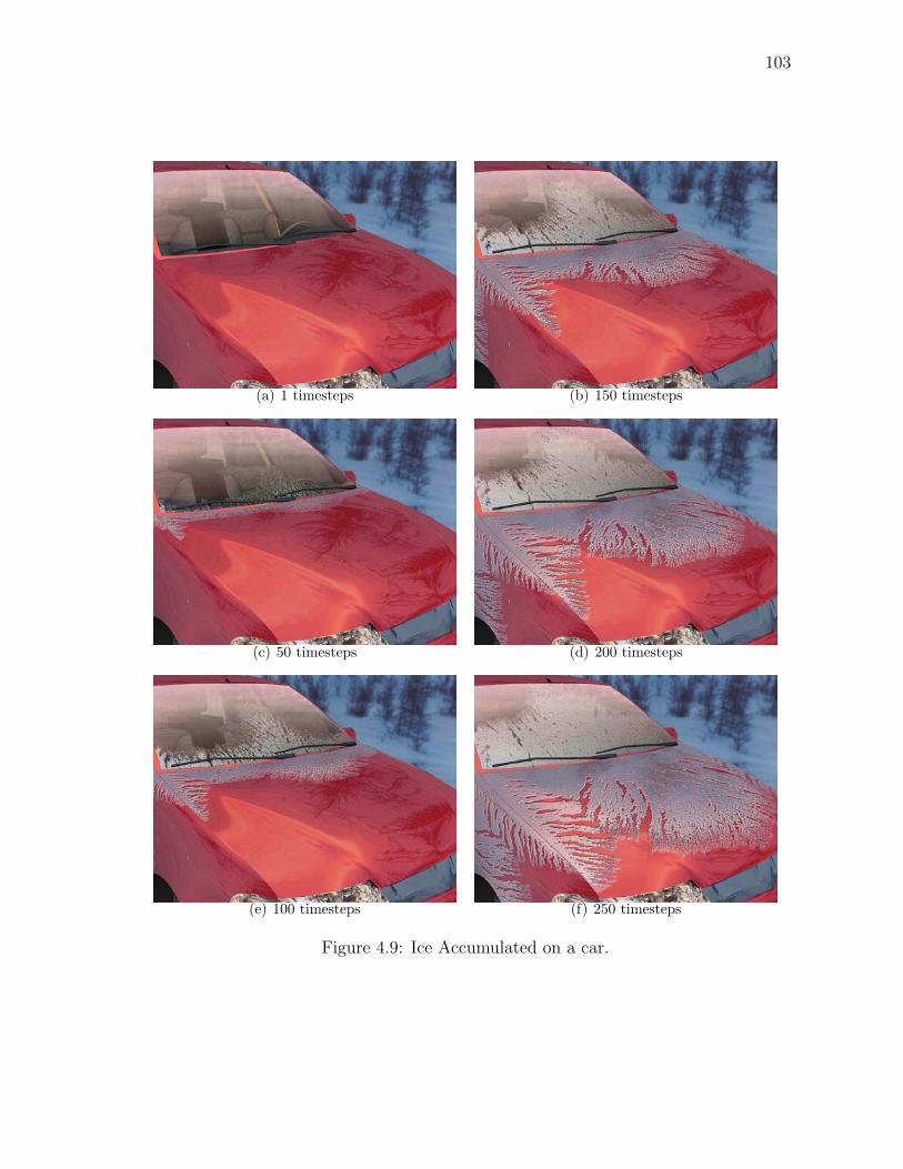
103

(a) 1 timesteps (b) 150 timesteps

(c) 50 timesteps (d) 200 timesteps

(e) 100 timesteps (f) 250 timesteps

Figure 4.9: Ice Accumulated on a car.

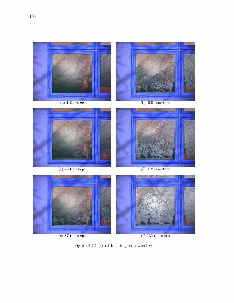
104

(a) 1 timestep (b) 100 timesteps

(c) 73 timesteps (d) 112 timesteps

(e) 87 timesteps (f) 132 timesteps

Figure 4.10: Frost forming on a window.

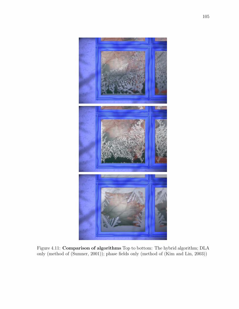
105

Figure 4.11: Comparison of algorithms Top to bottom: The hybrid algorithm; DLAonly (method of (Sumner, 2001)); phase fields only (method of (Kim and Lin, 2003))

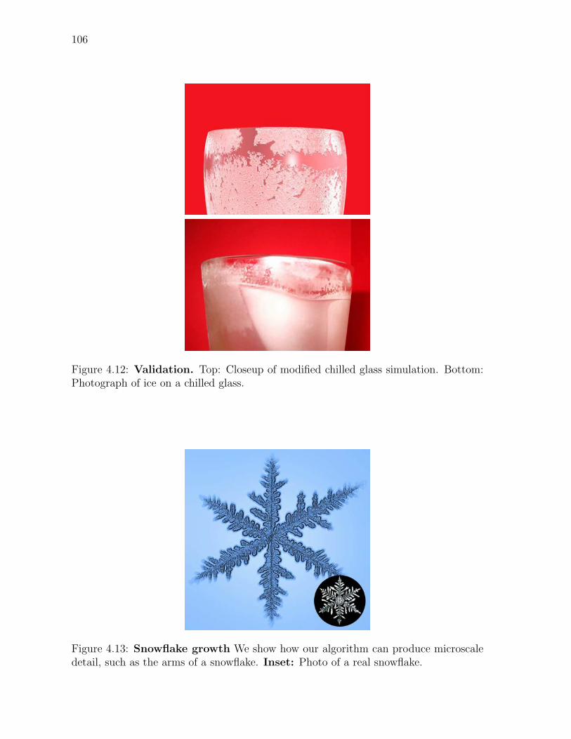
106

Figure 4.12: Validation. Top: Closeup of modified chilled glass simulation. Bottom:Photograph of ice on a chilled glass.

Figure 4.13: Snowflake growth We show how our algorithm can produce microscaledetail, such as the arms of a snowflake. Inset: Photo of a real snowflake.

Chapter 5

Icicle Growth

In previous chapters I described methods of simulating frost formation using a com-

bination of phase fields, diffusion limited aggregation (DLA), and stable fluid solvers.

While these techniques work well for flat, essentially 2D formations, they do not extend

naturally to 3D. Phase fields assume that the water supply in the environment is thick

and plentiful. In 3D, this would only be the case for something like a freezing lake,

which does not qualify as a ‘typical’ winter scene. DLA is essentially a model for va-

por deposition, and produces bushy, dendritic structures in 3D that do not bear close

resemblance to icicles.

However, the dense optical and geometric complexity of icicles adds appeal and

authenticity to any winter scene, so modeling their dynamics is an interesting and

worthwhile problem. Large icicle formations have appeared in such recent films as The

Incredibles and The Lion, the Witch and the Wardrobe. In the former, the icicles were

modeled as smooth, stylized cones, and in the latter, they had to be hand-molded from

plaster and clay. In the absence of a computational model for solidification, realistically

modeling these ice formations by hand can be a daunting task. This task becomes even

more demanding if an animation of the ice forming is required, as it is unclear what

the dynamics of the ice surface should be.

Extending existing graphics algorithms to faithfully simulate these dynamics is dif-

ficult, because the set of defining visual features is different. Recent research efforts

have found much success in simulating fluids (see e.g. (Selle et al., 2005) and (Feldman

108

et al., 2005) for recent results), but these algorithms are designed to capture features

such as vorticity and splashing. Freezing is instead characterized by sharp icicle tips,

and the optical effects caused by surface rippling. The underlying pattern formation

mechanisms are different from fluid dynamics, so different algorithms are needed. The

techniques from the previous chapter dealt with small-scale, essentially 2D formations

such as frost on surfaces or snowflakes. The techniques described assume that the ice

crystal is surrounded by a large bath of water, and while an argument can be made

that this is the case in 2D, it is clearly not the case in 3D. This makes their extension

to the complex 3D cases presented in this chapter difficult.

Simulating large scale ice formation is a challenging task due to the wide range of

scales involved. An interesting icicle formation is on the scale of roughly 1 meter, but

the tip of an icicle is roughly 2 millimeters in radius, and a thin water film coats the ice

that is on the order of tenths of a millimeter in thickness. The thin water layer drives

the formation of ripples, and the optics of these ripples give ice its characteristic look.

In this chapter, I present a method that captures these various multi-scale phenomena

in a single unified simulation.

In previous chapters, I first described a simulation method, and then drew a connec-

tion to the Stefan problem. For the formations presented in this chapter, there does not

appear to be any viable simulation method available, so I will instead derive one from

the original Stefan problem. Usually the Stefan problem examines how ice forms given

a virtually infinite supply of water. I am instead interested in the case encountered in a

typical wintery scene, where the water supply is severely limited. Therefore, I present

the ‘thin-film’ version of the Stefan problem and design a novel method for solving this

problem efficiently.

Features on the ice surface frequently merge, so I have elected to use level set

methods for the overall simulation (Osher and Fedkiw, 2003; Sethian, 1999). Level set

methods tend to smear out small-scale features, so I describe methods of tracking these

features separately. I derive an analytical solution for the dynamics of the icicle tip, as

well as a curvature-dependant evolution equation for the ice far from the tip. In order

109

to avoid explicitly tracking a large amount of ripple geometry, I modify an analytical

model from physics that poses surface ripples as a Fourier mode along the ice surface.

I use this method to defer explicit instantiation of the ripple geometry to render time,

which greatly simplifies the level set simulation.

5.1 The Stefan Problem

5.1.1 Background

In math and physics, solidification is usually posed as a Stefan problem. First posed by

Josef Stefan (Stefan, 1889) as a model of ocean ice forming in arctic regions, the Stefan

problem has since found applications in fields ranging from geology to metallurgy. The

richly non-linear behavior of the problem has also attracted considerable interest in

mathematics (Hill, 1987; Meirmanov, 1992). An excellent historical overview of the

Stefan problem is available in (Wettlaufer, 2001).

There are only a handful of known closed form solutions to the Stefan problem,

and these only apply to simple geometries. Stefan originally solved the planar case,

and subsequently the case of a sphere (Frank, 1949) and a parabola (Ivantsov, 1947)

were derived. These cases are often referred to eponymously as the “Frank sphere”

and “Ivantsov parabola” solutions. The derivations of these solutions are available in

Chapter 2, and discussed in detail by Saito (Saito, 1996). I will later base the thin film

equations on these solutions.

Due to its ability to handle geometry with rapidly changing topology, level set

methods have found recent success in solving the Stefan problem numerically. The

method was first applied in Sethian and Strain (Sethian and Strain, 1992) as a boundary

integral formulation, an alternate formulation was proposed by Chen et al. (Chen et al.,

1997) and this approach was later extended to second (Gibou et al., 2003) and fourth

order (Gibou and Fedkiw, 2005) accuracy. All of this work dealt with the classical

Stefan problem. I am instead interested in applying level set methods to the thin film

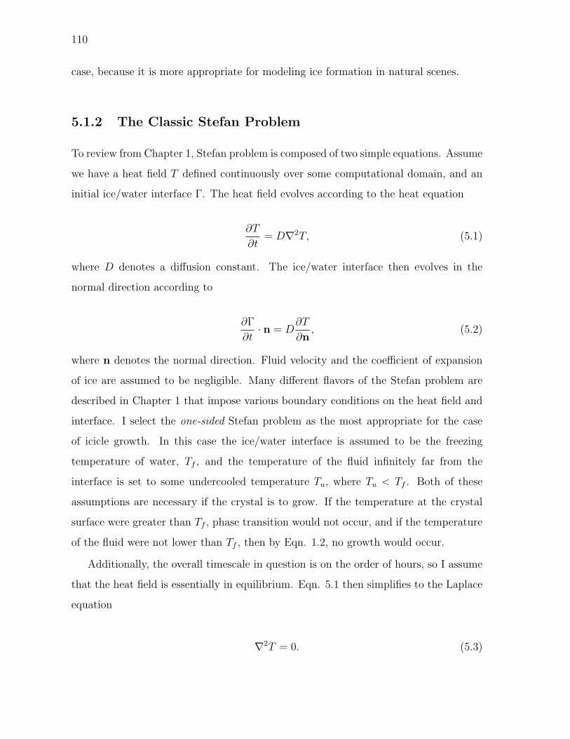
110

case, because it is more appropriate for modeling ice formation in natural scenes.

5.1.2 The Classic Stefan Problem

To review from Chapter 1, Stefan problem is composed of two simple equations. Assume

we have a heat field T defined continuously over some computational domain, and an

initial ice/water interface Γ. The heat field evolves according to the heat equation

∂T

∂t= D∇2T, (5.1)

where D denotes a diffusion constant. The ice/water interface then evolves in the

normal direction according to

∂Γ

∂t· n = D

∂T

∂n, (5.2)

where n denotes the normal direction. Fluid velocity and the coefficient of expansion

of ice are assumed to be negligible. Many different flavors of the Stefan problem are

described in Chapter 1 that impose various boundary conditions on the heat field and

interface. I select the one-sided Stefan problem as the most appropriate for the case

of icicle growth. In this case the ice/water interface is assumed to be the freezing

temperature of water, Tf , and the temperature of the fluid infinitely far from the

interface is set to some undercooled temperature Tu, where Tu < Tf . Both of these

assumptions are necessary if the crystal is to grow. If the temperature at the crystal

surface were greater than Tf , phase transition would not occur, and if the temperature

of the fluid were not lower than Tf , then by Eqn. 1.2, no growth would occur.

Additionally, the overall timescale in question is on the order of hours, so I assume

that the heat field is essentially in equilibrium. Eqn. 5.1 then simplifies to the Laplace

equation

∇2T = 0. (5.3)

111

Note that due to the absence of a timescale, the diffusion constant D can be dropped

in this case. This quasi-steady state approximation and the boundary conditions just

described are used in all the existing models from glaciology (Maeno et al., 1994;

Makkonen, 1988; Szilder and Lozowski, 1994) and physics (Ogawa and Furukawa, 2002;

Ueno, 2003) as well.

5.1.3 The Thin Film Stefan Problem

Unlike the classic Stefan problem, I want to model the situation where a thin film of

water continuously coats the outside of the ice. I assume that the crystal surface is at

freezing temperature Tf , but instead of specifying the undercooled temperature Tu at

some infinitely far away boundary, I specify it at a small offset δ from the interface.

More formally, I specify this as

Γ + δ(Γ · n) = Tu. (5.4)

Using this modified boundary condition, I derive thin-film evolution equations that can

be solved using level set methods.

The simplest case is an evolving planar interface. In 1D, Eqn. 5.4 simplifies to

Γ + δ = Tu. Assume that the plane is growing continually in the z direction. Within

this coordinate system, we define the current position of the interface as z′. The Laplace

equation at z′ then integrates to:

T (z′) =

(Tu − Tf

δz′ + Tf

). (5.5)

By inserting the result into Eqn. 1.2, we obtain a constant velocity for the planar

case:

dΓ

dt= D

Tu − Tf

δ. (5.6)

This planar solution matches the one obtained in (Ueno, 2003).

112

The cylindrical solution can be obtained in a manner similar to the classical solution

described in (Hill, 1987). For the cylindrical case, we must instead solve the polar

Laplace equation,

∂2T

∂r2+

1

r

∂T

∂r= 0, (5.7)

where r is the radial coordinate. We assume the crystal is growing in the positive r

direction, and define the current interface position as r′ within this coordinate system.

The exact method we use to transform Γ to r′ will be discussed later. The solution

must be of the form:

T (r) = A + B log r.

The thin film boundary conditions can be stated as:

T (r′) = Tf

T (r′ + δ) = Tu.

The constants then solve to:

A = Tf − Tu − Tf

log r′+δr′

log r′

B =Tu − Tf

log r′+δr′

Applying these two constants, we obtain

T (r′) = Tf +Tu − Tf

log(

r′+δr′

)(log r − log r′). (5.8)

We want a velocity equation at r′, so we take the derivative of Eqn. 5.8, solve for r = r′,

and substitute the result into Eqn. 1.2 to obtain:

113

∂Γ

∂t= D

∂T (r′)∂r

= DTu − Tf

r′ log(

r′+δr′

) . (5.9)

We can obtain a similar solution for the negative curvature case. This corresponds to

the case where the ice freezes radially inwards to fill in a cylindrical hole. Following

steps similar to those above, we obtain

∂Γ

∂t= −D

Tu − Tf

r′ log(

r′−δr′

) . (5.10)

Eqns. 5.9 and 5.10 can be consolidated into a single velocity equation,

∂Γ

∂t= D

Tu − Tf

|r′| log(|r′|+δ|r′|

) . (5.11)

This is the equation that the level set solver solves. Note this equation implicitly

includes Eqn. 5.6 as well. The planar case corresponds to the case of a cylinder of

infinite radius, and in the limit

limr′→∞

DTu − Tf

|r′| log(|r′|+δ|r′|

) = DTu − Tf

δ, (5.12)

the planar velocity equation is retrieved. Therefore, Eqn. 5.11 describes the interface

velocity of a positive and negative cylinder, as well as a plane. Note that Eqn. 5.11

contains a singularity at r′ = 0, but this is to be expected, as it corresponds to the

spurious physical case of a cylinder with zero radius.

5.1.4 The Thin Film Ivantsov Parabola

In this section I will derive a solution to the thin-film Stefan problem for parabolic

geometry. The paraboloid solution drives icicle growth, so it is crucial that it be solved

accurately. From a visual simulation standpoint, correctly capturing the velocity of

an icicle tip is important because it determines the overall shape of the icicle. If the

velocity is too slow, we will get unconvincingly stubby icicles, and if it is too fast, we

114

will get equally unconvincing needles.

The experimental measurements in Maeno et al. (Maeno et al., 1994) indicate that

across a wide range environmental conditions, the radius of the tip of an icicle remains

fixed at approximately 2.5 mm. If we are tracking features inside a 1 meter3 cube on a

regular grid, in order to resolve the tip using even an extremely coarse 43 neighborhood,

we need at least a 16003 grid. Even then, it is unclear if numerical smearing would

destroy the sharp tips.

I could use adaptive refinement to create a very fine grid around the tip, but I

opt for a simpler solution. By using an analytical solution for the growing icicle tip, I

can correct the signed distance function at every timestep. I am able to solve for the

dynamics of the icicle tip independently because the physics only depend on three local

factors: the curvature, the ice and air temperatures, and the size of the ‘pendant drop’

on the tip of the icicle.

In crystal growth, the Ivantsov parabola solution is often used to model the growing

tip of a dendrite. I conjecture that icicles are the thin film analogs of classic Stefan prob-

lem dendrites. There are several different methods of obtaining the Ivantsov parabola

solution, but I model the following thin-film derivation after the derivation given in

(Saito, 1996). Assume that a parabolic crystal is growing in the z direction with a

velocity V . Define a moving frame z′ = z− V t so that at time t, z′ = 0 always denotes

the current position of the parabola tip. We can then define a parabolic coordinate

system

ξ = r − z′

η = r + z′

θ = arctan(x/y),

where r =√

x2 + y2 + z′2. Intuitively, ξ and η each define a paraboloid in space, and

their intersection forms a circle. The θ coordinate then defines a point on this circle.

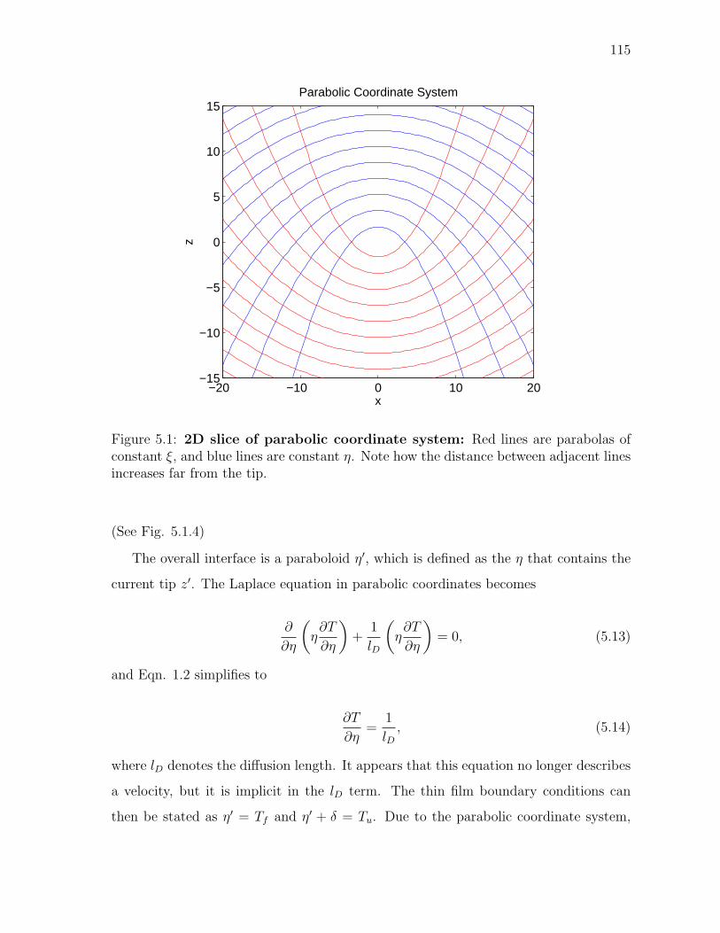
115

−20 −10 0 10 20−15

−10

−5

0

5

10

15Parabolic Coordinate System

x

z

Figure 5.1: 2D slice of parabolic coordinate system: Red lines are parabolas ofconstant ξ, and blue lines are constant η. Note how the distance between adjacent linesincreases far from the tip.

(See Fig. 5.1.4)

The overall interface is a paraboloid η′, which is defined as the η that contains the

current tip z′. The Laplace equation in parabolic coordinates becomes

∂

∂η

(η∂T

∂η

)+

1

lD

(η∂T

∂η

)= 0, (5.13)

and Eqn. 1.2 simplifies to

∂T

∂η=

1

lD, (5.14)

where lD denotes the diffusion length. It appears that this equation no longer describes

a velocity, but it is implicit in the lD term. The thin film boundary conditions can

then be stated as η′ = Tf and η′ + δ = Tu. Due to the parabolic coordinate system,

116

the second boundary condition is only meaningful near the tip. As shown in Fig.

5.1.4, the normal distance between two adjacent values of η increases as the distance

from the tip increases. Therefore, far from the tip, the distance between the two will

be much greater than δ. Fortunately, since we are only interested in values near the

tip, far away inaccuracies are irrelevant. Similar arguments are made when using the

Ivantsov parabola to approximate dendrite tips in crystal growth. In these cases, the

Ivantsov parabola obviously does not correctly model the side branches on a dendrite.

However, since these branches occur relatively far from the tip, the parabola is still

a reasonable approximation. Using these boundary conditions, the parabolic Laplace

equation integrates to

T (η) =Cp(Tu − Tf )

L

1−

∫ η

η′e− η

lD

η

∫ η′+δ

η′e− η

lD

η

. (5.15)

where L is the latent heat, and Cp is the specific heat. Inserting this result into Eqn.

5.14, we obtain

Cp(Tu − Tf )

L=

η′

lDe

η′lD

∫ η′+δ

η′

e− η

lD

η

=η′

lDe

η′lD

(∫ ∞

η′

e− η

lD

η−

∫ ∞

η′+δ

e− η

lD

η

).

(5.16)

By applying exponential integral notation E1(P ) =∫∞

Pe−x

xand a change of variables

using the Peclet number P = η′lD

, this equation can be rewritten as

Cp(Tu − Tf )

L= PeP

(E1(P )− E1

(P +

δ

lD

)). (5.17)

Velocity can be solved for by substituting the identity P = η′V2D

, where V is the tip

velocity and D is the thermal diffusitivity. Like the classic Ivantsov parabola solution,

Eqn. 5.17 is difficult to integrate explicitly, so I solve it numerically. Similar to the

method used in the classic case, I first approximate E1(P ) with its Puiseux series

117

symbol definition valueTf freezing temperature 0oCTu undercooled temperature −4.9oCL latent heat of fusion 3.3× 108 J/m3

D thermal diffusion constant 1.3× 10−7 m2/sCp specific heat 4.2× 106 J/(Km3)h0 thickness of water layer 10−4 mk wavenumber 600n solid over liquid thermal conductivities 3.92ε initial ripple amplitude 1× 10−4 mσr ripple amplification rate 5.2× 10−4 s−1

vp ripple translational velocity −6.1× 10−7 m/s

Table 5.1: Symbols and values. Values are from (Ueno, 2003).

E1(P ) = γ + ln P +n=1∑∞

(−1)nP n

n!n, (5.18)

where γ is the Euler-Mascheroni constant, and then solve for V using Newton iteration.

In contrast to Eqn. 5.17, the classic Ivantsov relation is

Cp(Tu − Tf )

L= PeP E1(P ),

so the thin film version adds an extra E1

(P + δ

lD

)term to account for the modified

boundary condition.

5.2 A Ripple Formation Model

The equations we have presented so far will produce sharp icicle tips, and smooth

features far from the tip. However, other non-smooth features occur in ice formations.

This is most visible as ripples along the surface of an icicle. In this section, we present

a method of simulating these features.

Until recently, the formation of these features was poorly understood. Pattern

formation of this type is usually explained in terms of Mullins-Sekerka theory (Mullins

118

and Sekerka, 1964), but Mullins-Sekerka theory predicts the formation of patterns at

all wavelengths, whereas experiments show that ice ripples only form at a wavelength

of roughly 1 cm. Recently, (Ueno, 2003) showed that one of the elements of Mullins-

Sekerka theory, the Gibbs-Thomson effect, does not apply in the case of ice ripple

formation, and proposed an alternate formation model.

The Ueno model can be stated in one dimension as

u(x, t) = εeσrt sin(k(x− vpt)), (5.19)

where x and t are spatial and temporal coordinates, ε is the amplitude of the initial

ripple, k is a wavenumber, and σr and vp are defined as

σr =V

h0

(−1.5αµPe + µ(36− 1.5αµPe)

36 + α2+

nµ−0.7αµPe− α2 + µ(36− 0.7αµPe)

36 + α2

) (5.20)

vp = −V

µ

(−0.25α2µPe + µ(6α + 9µPe)

36 + α2+

nµ6α− 7

60α2µPe + µ(6α + 21

5µPe)

36 + α2

).

(5.21)

Eqn. 5.19 describes a sine wave that amplifies in time according to σr and translates

in the negative x direction with a velocity vp. The remaining symbols are computed

according to the following formulas:

α = 2 cot θ · h0k + a2h0k3 (5.22)

µ = kh0 (5.23)

Pe =g sin θh4

0k

2κνµ(5.24)

a =

√2γ

gρ sin θ. (5.25)

Where κ = 1.3×10−7 m2/s, ν = 1.8×10−6 m2/s, γ = 7.6×10−2 N/m, ρ = 103 Kg/m3,

119

and g = 9.8 m/s2.

Intuitively, we can think of Eqn. 5.19 as a sine wave being transported along the

ice surface, which amplifies in time by a factor σr and climbs up the length of the icicle

with a velocity vp. The representation is attractive because allows us to track just a

single ‘creation time’ scalar during the simulation, and leave the instantiation of ripple

geometry to the renderer.

If we use Eqn. 5.19 directly in our simulation, unnaturally symmetric ripples are

obtained. This is because in the Ueno model, the translational velocity vp is assumed

to be constant. A brute force method of introducing more visual variety would be to

take the derivative of Eqn. 5.19 and integrate it at every grid point, at every timestep.

Such an equation would take the form:

dy

dt= δeσrt(σr sin(k(x− vpt))− kvp cos(k(x− vpt))). (5.26)

By applying a trigonometric identity, we can convert this to a Fourier mode of wavenum-

ber k.

dy

dt= δeσrt((σr cos(kvpt)− kvp sin(kvpt)) sin(kx)−

(kvp cos(kvpt) + σr sin(kvpt)) cos(kx))

(5.27)

However, using this equation would impose a small timestep restriction on the simula-

tion, and since the timescale in question is on the order of hours, I would like to avoid

such a restriction.

Instead, I observe that vp variable can be interpreted as the average translational

velocity of the interface over the lifetime of the ripple. Various environmental conditions

cause this average velocity to fluctuate over time, so I can imitate this physical noise

using numerical noise. I elect to use an easily controlled Perlin noise with a 1 cm

wavelength. At render time, each vertex does a lookup into a 3D Perlin noise function

and uses it to jitter vp. In addition to avoiding a timestep restriction, this approach also

decouples the small scale detail almost entirely from the level set simulation. When

120

designing ice patterns, the small scale ripple details can then be tweaked without having

to rerun the simulation.

5.3 A Level Set Solver

5.3.1 Background

I will now describe how to solve the equations from the previous sections using level

set methods (Osher and Fedkiw, 2003; Sethian, 1999). Level set methods can simulate

interfaces with rapidly changing topology by embedding the interface as an isosurface

in a higher-dimensional function, which is usually a signed distance function φ. The

function is then evolved according to the equation

∂φ

∂t+ v · ∇φ = 0, (5.28)

where v is some velocity field. Because the ice interface often merges, I have decided

to use level set methods in this work. I specifically use the narrow band level set

method (Adalsteinsson and Sethian, 1995a), where the narrow band is tracked using

an unbalanced octree, much as in Losasso et al. (Losasso et al., 2004).

For the spatial derivatives, I use a fifth order Hamilton Jacobi Weighted Essentially

Non-Oscillatory (HJ-WENO) scheme (Liu et al., 1996). In its simplest form, level set

methods use first order upwinding to timestep the simulation. The usual method of

obtaining a second order accurate derivative would be to take a weighted average of

both the upwind and downwind neighbors. However, while this discretization accounts

for more terms in the Taylor expansion, from a physical standpoint it is incorrect.

Using downwind information to estimate what is fundamentally an upwind quantity

only introduces unrelated information into the computation. Higher order methods can

then be obtained by using more neighbors from the upwind direction.

Using strictly upwind neighbors can lead to problems in some cases, because if

the stencil crosses a discontinuity, spuriously large derivatives can be obtained. Es-

121

sentially Non-Oscillatory (ENO) schemes (Harten et al., 1987) are a method of de-

tecting such discontinuities that decides when to use to upwind neighbors and when

downwind neighbors will suffice. Using ENO schemes, third order accuracy can be

achieved. Whereas ENO schemes select only one set of neighboring points to estimate

the derivative, Weighted ENO (WENO) schemes use a weighted combination of all

possible neighboring point sets. In this manner, fifth order accuracy is obtained.

In my simulations, there are substantial discontinuities in the distance field near the

medial axis of the icicles. This is not a problem once the icicles have grown sufficiently

thick that their derivative stencils no longer use grid cells near the medial axis, but

when the icicle is initially forming, this can cause spuriously noisy results. By using a

HJ-WENO scheme, these artifacts are greatly reduced.

For the time discretization, I used second order timestepping via the midpoint

rule. Fluid simulation techniques in graphics usually use Total Variational Diminishing

Runge Kutta (TVD-RK), but for second order accuracy TVD-RK reduces to midpoint

rule. I have found that using this scheme also appears to give results that are less prone

to spurious numerical noise.

In graphics, a hybrid particle level set method (Enright et al., 2002a) has recently

been successful in simulating the Navier-Stokes equations because it uses Lagrangian

particles to re-introduce smeared out small scale detail. In this chapter, I capture the

small scale detail using alternate methods, so a basic level set solver suffices.

5.3.2 The Velocity Field

In order to evolve an existing ice interface, we must specify a velocity v. I choose

to approximate the interface as locally cylindrical, and use Eqn. 5.11 to compute a

velocity in the normal direction. I plug the maximum principal curvature at each grid

point into r′, since this describes essentially the largest osculating cylinder at that

point. Sethian (Sethian, 1999) describes the following method of computing Gaussian

curvature K and mean curvature H in level sets:

122

K =φ2

x(φyyφzz − φ2yz) + φ2

y(φxxφzz − φ2xz) + φ2

z(φxxφyy − φ2xy)

(φ2x + φ2

y + φ2z)

2+

2(φxφy(φxzφyz − φxyφzz) + φyφz(φxyφxz − φyzφxx) + φxφz(φxyφyz − φxzφyy))

(φ2x + φ2

y + φ2z)

2

and

H =(φyy + φzz)φ

2x + (φxx + φzz)φ

2y + (φxx + φzz)φ

2y

(φ2x + φ2

y + φ2z)

2

− 2(φxφyφxy + φxφzφxz + φyφzφyz)

(φ2x + φ2

y + φ2z)

2.

The maximum principal curvature can then be computed as the larger root κ of the

quadratic κ2 − 2Hκ + K = 0.

Eqn. 5.11 is only defined along the interface, whereas we require velocities over

the entire narrow band. Since curvature is defined over the entire domain, I use it to

compute values for Eqn. 5.11 everywhere. This approach does not seem to distort the

distance field too badly, so it works well in practice.

Robust curvature information is crucial to obtaining meaningful velocities, but as

curvature is a second order geometric quantity, a first order reinitialization scheme can

create spurious curvature values at the interface. While curvature in level set methods

can be noisy in general, first order reinitialization can produce garbage values. Trivially

incorrect values can commonly occur, such as negative curvature in convex regions and

vice versa.

Sethian (Sethian, 1999) describes a second order reinitialization method, but this

is only second order for φ overall; it is still first order accurate at the interface. In

order to achieve fully second order reinitialization, I use the reinitialization method

described by Chopp (Chopp, 2001). Chopp achieves fully second order accurate fast

marching by locally fitting a cubic interpolant over a 43 neighborhood at each grid

point adjacent to the interface. The weights of this cubic interpolant are obtained

by solving a linear system at each grid point. Fortunately, the system is insensitive

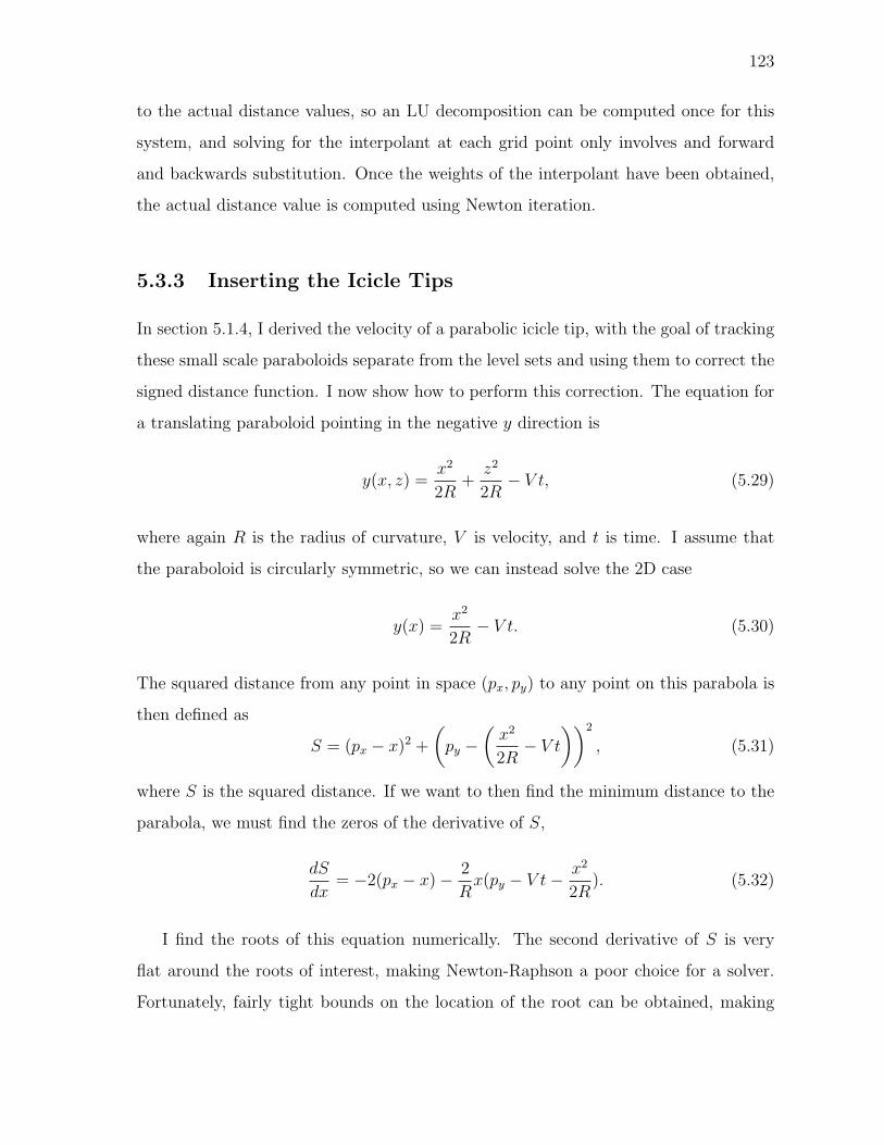
123

to the actual distance values, so an LU decomposition can be computed once for this

system, and solving for the interpolant at each grid point only involves and forward

and backwards substitution. Once the weights of the interpolant have been obtained,

the actual distance value is computed using Newton iteration.

5.3.3 Inserting the Icicle Tips

In section 5.1.4, I derived the velocity of a parabolic icicle tip, with the goal of tracking

these small scale paraboloids separate from the level sets and using them to correct the

signed distance function. I now show how to perform this correction. The equation for

a translating paraboloid pointing in the negative y direction is

y(x, z) =x2

2R+

z2

2R− V t, (5.29)

where again R is the radius of curvature, V is velocity, and t is time. I assume that

the paraboloid is circularly symmetric, so we can instead solve the 2D case

y(x) =x2

2R− V t. (5.30)

The squared distance from any point in space (px, py) to any point on this parabola is

then defined as

S = (px − x)2 +

(py −

(x2

2R− V t

))2

, (5.31)

where S is the squared distance. If we want to then find the minimum distance to the

parabola, we must find the zeros of the derivative of S,

dS

dx= −2(px − x)− 2

Rx(py − V t− x2

2R). (5.32)

I find the roots of this equation numerically. The second derivative of S is very

flat around the roots of interest, making Newton-Raphson a poor choice for a solver.

Fortunately, fairly tight bounds on the location of the root can be obtained, making

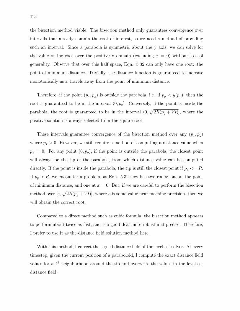
124

the bisection method viable. The bisection method only guarantees convergence over

intervals that already contain the root of interest, so we need a method of providing

such an interval. Since a parabola is symmetric about the y axis, we can solve for

the value of the root over the positive x domain (excluding x = 0) without loss of

generality. Observe that over this half space, Eqn. 5.32 can only have one root: the

point of minimum distance. Trivially, the distance function is guaranteed to increase

monotonically as x travels away from the point of minimum distance.

Therefore, if the point (px, py) is outside the parabola, i.e. if py < y(px), then the

root is guaranteed to be in the interval 〈0, px]. Conversely, if the point is inside the

parabola, the root is guaranteed to be in the interval 〈0, √2R(py + V t)], where the

positive solution is always selected from the square root.

These intervals guarantee convergence of the bisection method over any (px, py)

where px > 0. However, we still require a method of computing a distance value when

px = 0. For any point (0, py), if the point is outside the parabola, the closest point

will always be the tip of the parabola, from which distance value can be computed

directly. If the point is inside the parabola, the tip is still the closest point if py <= R.

If py > R, we encounter a problem, as Eqn. 5.32 now has two roots: one at the point

of minimum distance, and one at x = 0. But, if we are careful to perform the bisection

method over [ε,√

2R(py + V t)], where ε is some value near machine precision, then we

will obtain the correct root.

Compared to a direct method such as cubic formula, the bisection method appears

to perform about twice as fast, and is a good deal more robust and precise. Therefore,

I prefer to use it as the distance field solution method here.

With this method, I correct the signed distance field of the level set solver. At every

timestep, given the current position of a paraboloid, I compute the exact distance field

values for a 43 neighborhood around the tip and overwrite the values in the level set

distance field.

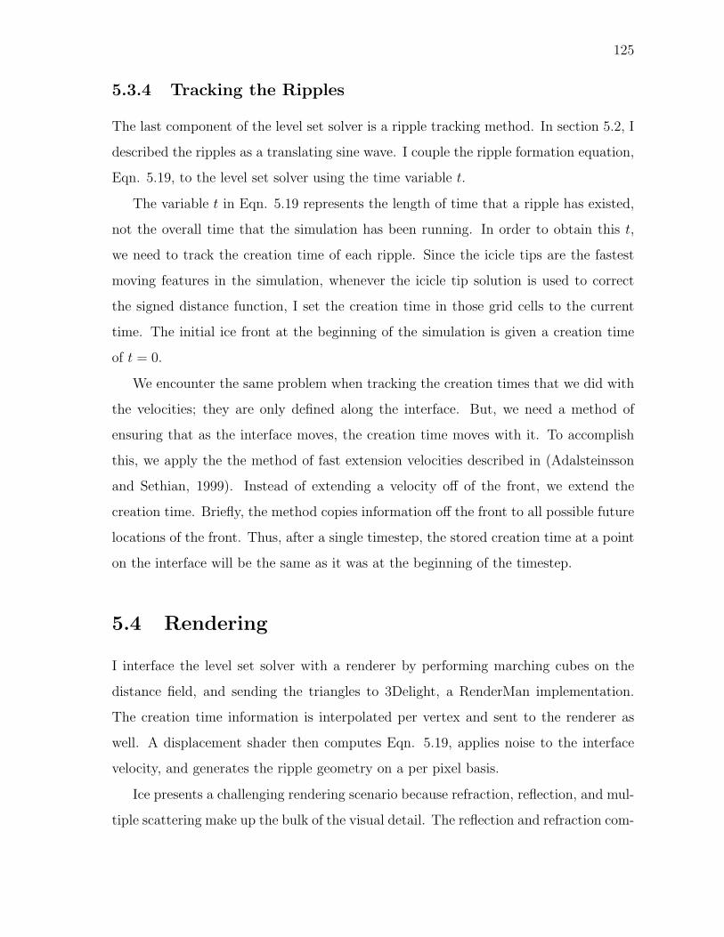
125

5.3.4 Tracking the Ripples

The last component of the level set solver is a ripple tracking method. In section 5.2, I

described the ripples as a translating sine wave. I couple the ripple formation equation,

Eqn. 5.19, to the level set solver using the time variable t.

The variable t in Eqn. 5.19 represents the length of time that a ripple has existed,

not the overall time that the simulation has been running. In order to obtain this t,

we need to track the creation time of each ripple. Since the icicle tips are the fastest

moving features in the simulation, whenever the icicle tip solution is used to correct

the signed distance function, I set the creation time in those grid cells to the current

time. The initial ice front at the beginning of the simulation is given a creation time

of t = 0.

We encounter the same problem when tracking the creation times that we did with

the velocities; they are only defined along the interface. But, we need a method of

ensuring that as the interface moves, the creation time moves with it. To accomplish

this, we apply the the method of fast extension velocities described in (Adalsteinsson

and Sethian, 1999). Instead of extending a velocity off of the front, we extend the

creation time. Briefly, the method copies information off the front to all possible future

locations of the front. Thus, after a single timestep, the stored creation time at a point

on the interface will be the same as it was at the beginning of the timestep.

5.4 Rendering

I interface the level set solver with a renderer by performing marching cubes on the

distance field, and sending the triangles to 3Delight, a RenderMan implementation.

The creation time information is interpolated per vertex and sent to the renderer as

well. A displacement shader then computes Eqn. 5.19, applies noise to the interface

velocity, and generates the ripple geometry on a per pixel basis.

Ice presents a challenging rendering scenario because refraction, reflection, and mul-

tiple scattering make up the bulk of the visual detail. The reflection and refraction com-

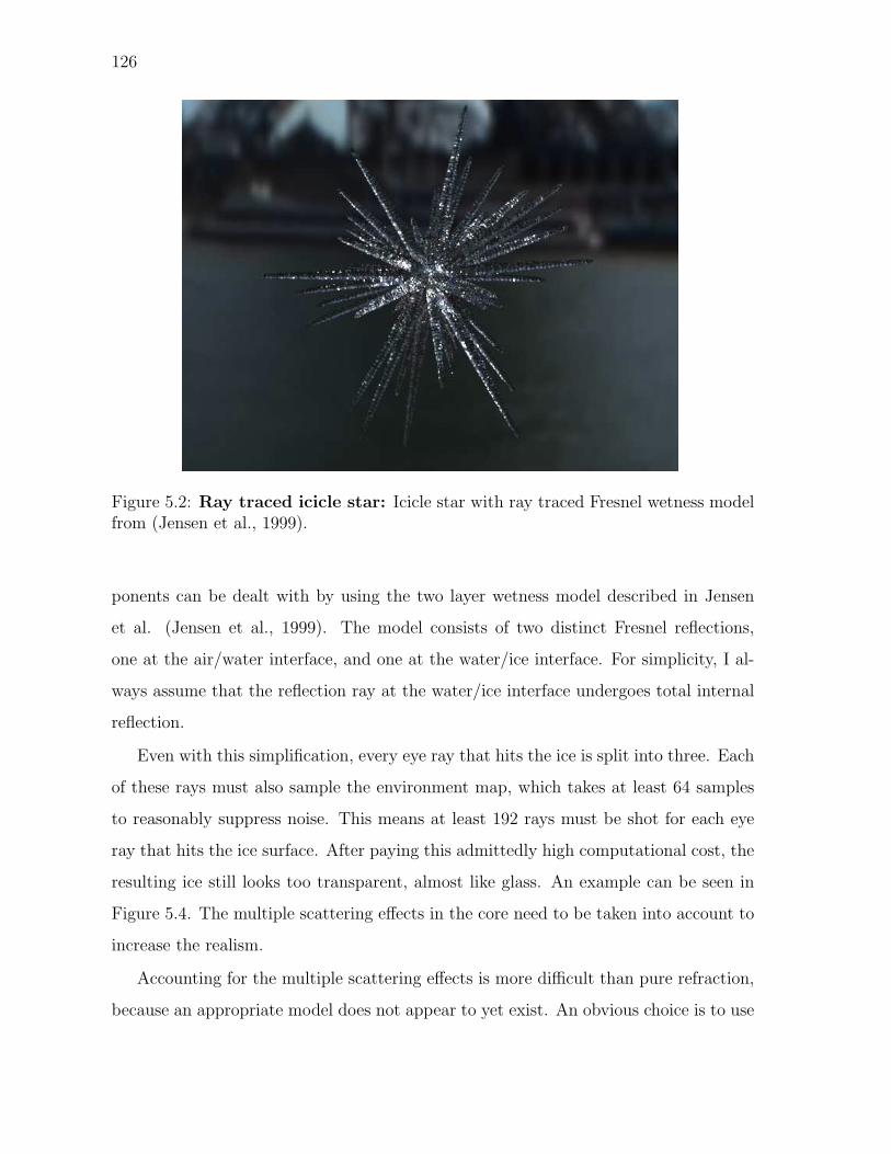
126

Figure 5.2: Ray traced icicle star: Icicle star with ray traced Fresnel wetness modelfrom (Jensen et al., 1999).

ponents can be dealt with by using the two layer wetness model described in Jensen

et al. (Jensen et al., 1999). The model consists of two distinct Fresnel reflections,

one at the air/water interface, and one at the water/ice interface. For simplicity, I al-

ways assume that the reflection ray at the water/ice interface undergoes total internal

reflection.

Even with this simplification, every eye ray that hits the ice is split into three. Each

of these rays must also sample the environment map, which takes at least 64 samples

to reasonably suppress noise. This means at least 192 rays must be shot for each eye

ray that hits the ice surface. After paying this admittedly high computational cost, the

resulting ice still looks too transparent, almost like glass. An example can be seen in

Figure 5.4. The multiple scattering effects in the core need to be taken into account to

increase the realism.

Accounting for the multiple scattering effects is more difficult than pure refraction,

because an appropriate model does not appear to yet exist. An obvious choice is to use

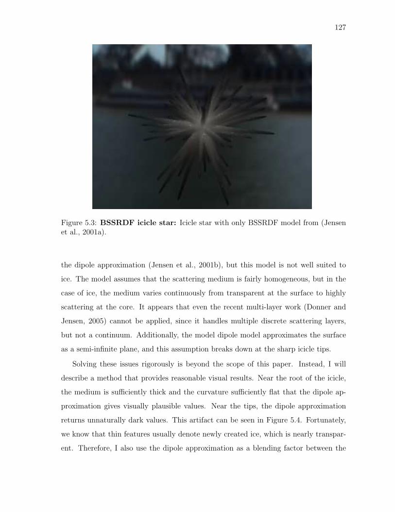
127

Figure 5.3: BSSRDF icicle star: Icicle star with only BSSRDF model from (Jensenet al., 2001a).

the dipole approximation (Jensen et al., 2001b), but this model is not well suited to

ice. The model assumes that the scattering medium is fairly homogeneous, but in the

case of ice, the medium varies continuously from transparent at the surface to highly

scattering at the core. It appears that even the recent multi-layer work (Donner and

Jensen, 2005) cannot be applied, since it handles multiple discrete scattering layers,

but not a continuum. Additionally, the model dipole model approximates the surface

as a semi-infinite plane, and this assumption breaks down at the sharp icicle tips.

Solving these issues rigorously is beyond the scope of this paper. Instead, I will

describe a method that provides reasonable visual results. Near the root of the icicle,

the medium is sufficiently thick and the curvature sufficiently flat that the dipole ap-

proximation gives visually plausible values. Near the tips, the dipole approximation

returns unnaturally dark values. This artifact can be seen in Figure 5.4. Fortunately,

we know that thin features usually denote newly created ice, which is nearly transpar-

ent. Therefore, I also use the dipole approximation as a blending factor between the

128

the multiple scattering color and the purely refracted ray color.

5.5 Results and Validation

I have used the described algorithm to simulate ice formation in several scenes, and

also validated portions of the model against experimental data. The code was compiled

using ICL 8, and the timings were obtained on a 3 Ghz Pentium 4. All simulations

take place on a virtual 2563 grid.

In Figure 5.7 I simulated ice forming on a fountain. The fountain was left running

during a cold day, and the overflowing water froze into ice. In order to introduce visual

variety into the icicles, I jittered the position of each icicle tip by 1 mm each timestep.

The simulation averaged 12 seconds a timestep and completed in 30 minutes. The

natural handling of merging icicles is visible in this scene, as well the straightforward

handling of boundary conditions. Growth is prohibited on the inside of the fountain

by merely clamping ∂φ∂t

= 0 on the interior of the fountain. Aside from specifying the

initial growth locations, the scene was modeled with a minimum of user intervention.

The icicle tips were inserted at random locations along the edge of the growing front.

In Figure 5.8 I simulated ice forming on a rooftop. The icicles were jittered by 1 mm

in this case as well. The simulation averaged 2.5 seconds a timestep and completed in 5

minutes. This scene was also modeled with a minimum of user intervention. The initial

growth position was specified along the rain gutter, and icicle tips were then placed

at random along its length. A Halton sequence pseudo-random number generator was

needed to obtain a good distribution however.

In order to demonstrate the flexibility of the model, I simulated an Andy Goldswor-

thy (Goldsworthy, 1990) sculpture in Figure 5.5. Mr. Goldworthy is an artist who

constructs sculptures from natural materials, in this case a star made of real icicles.

This formation could not occur naturally, because gravity forces a downwards water

flow. However, our model implicitly flow water in any direction by re-orienting the

parabolic tips. For an animation of this ‘zero-gravity’ star growing, see the attached

129

video. The simulation averaged 5.1 seconds per timestep and completed in 18 minutes.

Again, a minimum of user intervention was required, and icicle tips were placed along

the surface of the initial sphere using a spherical Halton sequence (Wong et al., 1997).

I have not found Eqn. 5.17 elsewhere in the literature, so to test its validity we have

compared it against experimental data. There is a limited amount of data available on

the type of ice growth I am modelling, but Maeno et al. (Maeno et al., 1994) provides

experimental data on icicle tip velocities under a range of undercoolings. In order to

make a comparison to their data, I must select appropriate values for η′ and δ. The η′

value can be interpreted as the radius of curvature of the icicle tip. As stated earlier,

experiments show that this value is 2.5 mm. The availability and stability of this value

is quite fortunate, because as mentioned in Chapter 2, the Ivantsov relation can only

solve for the product of the radius and velocity, not the velocity itself. Considerable

research effort has gone into imposing an additional constraint that can separate these

two quantities, giving rise to a so-called ‘solvability theory’. However, in the presence

of a stable, experimentally observed value, I do not need to appeal to any such theory.

The value of δ on the icicle surface is usually on the order of 1 × 10−4 m, but

this value represents the water thickness along the icicle wall, not at the tip. At the

tip, a pendant drop forms that is roughly the same radius as the underlying crystal.

Therefore, I estimate the value of δ at the tip to be 2.5 mm as well.

Fig. 5.5 shows how the predicted values compare to experimental data. I compute

tip velocities over a variety of undercoolings, and compare the results to those of the

classic Ivantsov relation. As stipulated by Eqn. 1.2, as the undercooling increases, the

growth rate must increase as well. The classic solution predicts much slower growth

and consistently undershoots the data. This is to be expected, because in the classic

case, the temperature gradient at the tip has been ‘stretched’ by the infinitely far away

boundary condition. While this experimental data set appears to be quite noisy, the

thin-film solution appears to be in fair agreement, and I have found that it generates

visually convincing results.

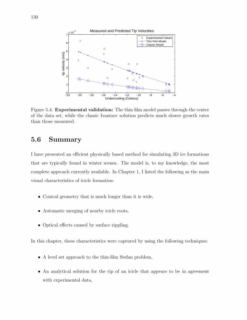
130

−22 −20 −18 −16 −14 −12 −10 −8 −6 −40

1

2

3

4

5

6

7x 10

−5 Measured and Predicted Tip Velocities

Undercooling (Celsius)

tip v

eloc

ity (

m/s

)

Experimental ValuesThin Film ModelClassic Model

Figure 5.4: Experimental validation: The thin film model passes through the centerof the data set, while the classic Ivantsov solution predicts much slower growth ratesthan those measured.

5.6 Summary

I have presented an efficient physically based method for simulating 3D ice formations

that are typically found in winter scenes. The model is, to my knowledge, the most

complete approach currently available. In Chapter 1, I listed the following as the main

visual characteristics of icicle formation:

• Conical geometry that is much longer than it is wide,

• Automatic merging of nearby icicle roots,

• Optical effects caused by surface rippling.

In this chapter, these characteristics were captured by using the following techniques:

• A level set approach to the thin-film Stefan problem,

• An analytical solution for the tip of an icicle that appears to be in agreement

with experimental data,

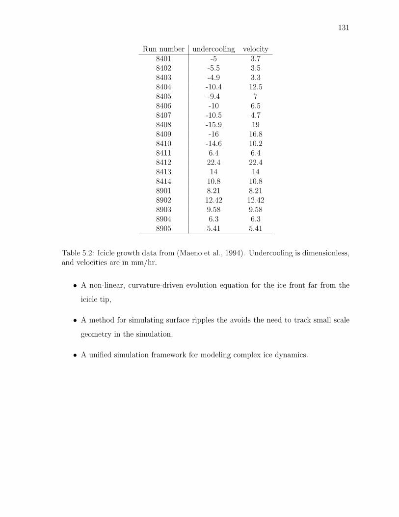
131

Run number undercooling velocity8401 -5 3.78402 -5.5 3.58403 -4.9 3.38404 -10.4 12.58405 -9.4 78406 -10 6.58407 -10.5 4.78408 -15.9 198409 -16 16.88410 -14.6 10.28411 6.4 6.48412 22.4 22.48413 14 148414 10.8 10.88901 8.21 8.218902 12.42 12.428903 9.58 9.588904 6.3 6.38905 5.41 5.41

Table 5.2: Icicle growth data from (Maeno et al., 1994). Undercooling is dimensionless,and velocities are in mm/hr.

• A non-linear, curvature-driven evolution equation for the ice front far from the

icicle tip,

• A method for simulating surface ripples the avoids the need to track small scale

geometry in the simulation,

• A unified simulation framework for modeling complex ice dynamics.

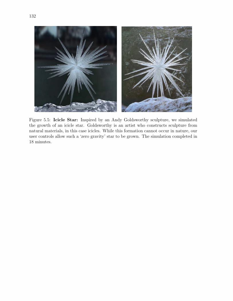
132

Figure 5.5: Icicle Star: Inspired by an Andy Goldsworthy sculpture, we simulatedthe growth of an icicle star. Goldsworthy is an artist who constructs sculpture fromnatural materials, in this case icicles. While this formation cannot occur in nature, ouruser controls allow such a ‘zero gravity’ star to be grown. The simulation completed in18 minutes.

133

(a) 0 timesteps (b) 120 timesteps

(c) 30 timesteps (d) 150 timesteps

(e) 60 timesteps (f) 180 timesteps

(g) 90 timesteps (h) 210 timesteps

Figure 5.6: Icicle star forming: Frames from the icicle star forming.

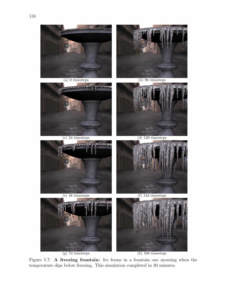
134

(a) 0 timesteps (b) 96 timesteps

(c) 24 timesteps (d) 120 timesteps

(e) 48 timesteps (f) 144 timesteps

(g) 72 timesteps (h) 168 timesteps

Figure 5.7: A freezing fountain: Ice forms in a fountain one morning when thetemperature dips below freezing. This simulation completed in 30 minutes.

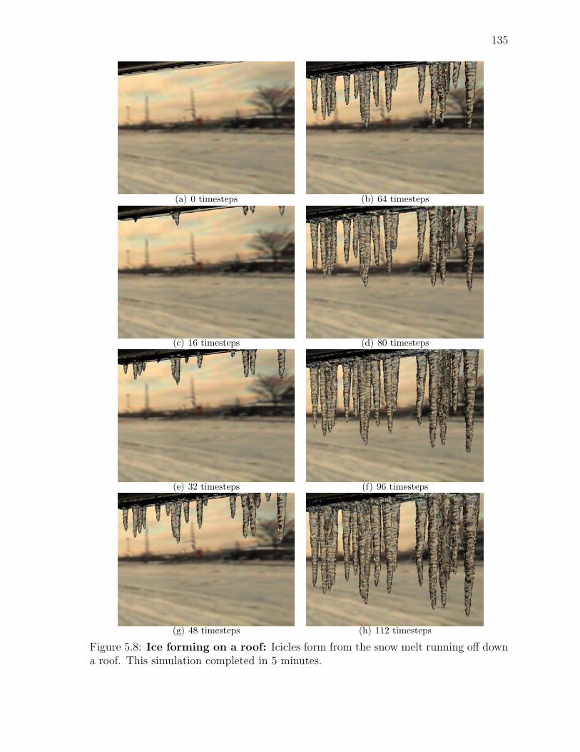
135

(a) 0 timesteps (b) 64 timesteps

(c) 16 timesteps (d) 80 timesteps

(e) 32 timesteps (f) 96 timesteps

(g) 48 timesteps (h) 112 timesteps

Figure 5.8: Ice forming on a roof: Icicles form from the snow melt running off downa roof. This simulation completed in 5 minutes.

136

Chapter 6

Conclusion

In this dissertation, I have presented several methods of simulating the formation of

ice. A rich variety of visual phenomena arise from solidification under different physical

conditions, and different methods are necessary to capture each of these situations. The

methods I presented are sufficiently distinct that they require unique computational

considerations, but physically, all of the approaches can be understood in the context

of the Stefan problem.

6.1 Summary of Results

I have presented the phase field method in the context of visual simulation. The phase

field method is derived from free energy equations, and can generate a wide variety of

patterns that span both the sectored plate and dendritic growth regimes. The phase

field method is an Eulerian simulation technique that can be computationally intensive,

so I have presented three optimization methods to reduce this workload. First, the phase

field equations are only non-zero around the neighborhood of the ice/water interface,

so computation can be restricted to a band around this interface. Second, the Eulerian

simulation grid maps naturally to textures on the GPU, so the SIMD nature of the phase

field simulation can be exploited by using graphics hardware. Finally, by ignoring the

off-diagonal terms of the diffusion tensor in the phase field equations, the diffusion

operator can be made entirely implicit, allowing larger timesteps to be taken.

138

The Eulerian nature of the phase field method allows it to handle topological change

naturally and maps easily to the GPU. However, these advantages come at a cost, be-

cause Eulerian grids typically suffer from smoothing artifacts. I proposed two different

methods of dealing with these artifacts. First, I described a physically-inspired method

of introducing crease detail along the medial axis of the simulation results. Second,

by examining the process of solidification, I proposed a physically-based method of

integrating phase fields with a Lagrangian particle-based algorithm known as Diffusion

Limited Aggregation (DLA). Lagrangian simulations can be viewed as the dual of Eu-

lerian simulations, and suffer from the opposite problem. Whereas Eulerian simulation

suffers from smoothing, Lagrangian simulation produces unnaturally sharp features.

By combining the two methods, I obtained an algorithm that combines the advantages

of both methods. In order to take into account the influence of wind flow in the sur-

rounding environment, I also described a method of integrating a fluid simulation into

both the phase field and DLA simulations.

Finally, I described a method of simulating the formation of icicles by phrasing the

formation mechanisms as a thin-film Stefan problem. There are no existing simulation

models that capture the visual characteristics of icicles, so I derived the relevant veloc-

ity equations for a level set simulation. I also described a method of simulating ripple

formation that avoids tracking a large amount of small scale geometry while also avoid-

ing additional timestep restrictions. The resulting algorithm is quite efficient, with all

of the presented simulations completing in a matter of minutes.

6.2 Limitations

All of the presented simulation methods capture their respective visual characteristics

effectively, but these methods also have limitations.

139

6.2.1 Phase Fields and DLA

Despite the optimizations presented for phase fields, they still remain fairly computa-

tionally intensive. Ideally an unconditionally stable version would be derived, allowing

arbitrarily large timesteps to be taken. This is difficult due to the presence of the ∂p∂t

term in Eqn. 3.1. A linearization may be possible that circumvents this term. It is

possible that an analytic patch such as that use in Chapter 5 may also be used on a

coarse grid to track sharp features, thus reducing the computational workload. Even

if an unconditionally stable scheme is derived, the large timesteps would undoubtedly

introduce smoothing artifacts. Stable fluids (Stam, 1999b) suffers from vorticity damp-

ing, an issue that was addressed using a CFD technique called vorticity confinement

(Fedkiw et al., 2001). A similar technique would probably need to be developed for

phase fields.

As it is used in Chapter 4, DLA is restricted to have anisotropy aligned with the

underlying grid. In nature, formations may display anisotropy in a local sense, but

they do not appear to be aligned on any sort of global grid. In other words, while

dendrites may all display six-armed anisotropy, the actual θ angles that the arms take

will differ from case to case. This limitation could perhaps be dealt with by use of

multiple grids with different alignments, although the additional bookkeeping would

significantly complicate implementation. Recent work (Bogoyavlenskiy, 2001) describes

a method of removing grid anisotropy entirely from a on-lattice DLA simulation. Once

these effects have been removed, it may be possible to introduce arbitrary anisotropy

functions. More work is necessary to determine if this is in fact the case.

The running time of DLA can also be problematic, as it involves a Monte Carlo step

whose time complexity is difficult to bound. Alternate methods such as the dielectric

breakdown model (DBM) presented in Chapter 4 or more recent conformal mapping

methods (Hastings and Levitov, 1998) may offer a method of accelerating computation.

Many acceleration techniques have been proposed for DLA, so incremental performance

gains are available via these techniques as well. Some of these methods, such as the

method of hierarchical maps (Ball and Brady, 1985), assume that the existing cluster

140

has been preprocessed into a tree data structure. This preprocess becomes significantly

more complicated in the context of the hybrid algorithm from Chapter 4 because the

phase field simulation evolves the cluster as well. A good deal of the coherence that the

hierarchical maps approach assumes is therefore broken. While it may be possible for

the phase field simulation to incrementally update the tree data structure, additional

work is necessary to determine the specifics of such an update.

6.2.2 Icicle Simulation

The icicle growth model presented in Chapter 5 derives a good deal of its speed ad-

vantage from the fact that it does not explicitly handle the water flow over the surface

of the ice. While this enables the simulation to take very large timesteps, it also lim-

its the types of growth that the simulation can handle. In particular, the thickness

of the water layer along the surface of the icicle is assumed to be constant over the

lifetime of the simulation. In nature, this is not always true, and different thicknesses

give rise to different visual phenomena. Icicles can shield other icicles from water flow,

creating different growth conditions that could halt growth in some regions altogether.

Additionally, wind forces can also influence the final shape of the icicle, stretching the

profile of the icicle into a ‘blade’ shape, or curving the path of the icicle tip. It may

be possible to capture these effects without introducing an explicit water simulation.

From a user control standpoint, a water thickness may be assigned to each icicle tip as

it is inserted, generating more visual variety. A more physically based approach would

be to compute something analogous to an ambient occlusion term (Landis, 2002) for

each portion of the icicle surface, and then estimate a water inflow rate based on the

amount of occlusion from other icicles.

Formations analogous to stalagmites usually form beneath icicles where the pendant

drop continually dripped to form a roughly conical formation. Since I do not explicitly

model water flow, these formations will need additional work to capture. They do not

appear to be a straightforward extension of the treatment used in Chapter 5 however,

because the water supply is a steady drip, not a thin film. Visually similar ‘drip castle’

141

formations were presented by Carlson et al. (Carlson et al., 2002), so similar techniques

can perhaps be applied to the case of ice formation as well.

There are still some ice formation phenomena that the techniques in this disserta-

tion cannot capture. Hoarfrost is the case where frost forms in large plates that jut

out from the surface of objects. This case of solidification is somewhere between the

frost formations handled by phase fields and the icicle formations handled by level sets.

Locally, hoarfrost is planar, but globally it is fully 3D, extending from frozen surfaces

in thornlike formations. While hoarfrost is not uncommon in winter scenes, it is un-

common enough that the average viewer does not ‘expect’ to see it. A new simulation

method would most likely need to be designed to handle this case, but the overall visual

realism would be minimally impacted, so I chose not to address it in this dissertation.

6.2.3 Rendering Issues

A drawback of all of the methods described in this thesis is that an efficient, physically

based rendering method is not currently available. While the goal of this dissertation

is simulation and not rendering, the two problems are interrelated, because a full ren-

dering solution may require additional information from the simulation. The sparkling,

spectrally dispersive reflections of frost may require mesofacet information from the

phase field and DLA simulations that they currently cannot resolve. While the role of

microfacets in reflection (Cook and Torrance, 1982) and efficiently rendering the rain-

bow effects of diffraction (Stam, 1999a) have been addressed in the past, the glittering

reflections off of frost are not a direct extension of either case, so additional work is

necessary. I observed in Chapter 5 that the multiple scattering properties of icicles are

inhomogeneous and continuously vary throughout the icicle volume. The variance of

these scattering parameters are not currently tracked anywhere in the simulation, and

for a full physically based rendering algorithm to be effective, this information may

become necessary. The physical mechanisms that give rise to this variance in scatter-

ing are unclear however, so computing and tracking these quantities is more than a

straightforward extension of the work presented here.

142

6.3 Future Work

Assuming the limitations described above are overcome, there still remains the problem

of user interaction. In the prototype systems described in the thesis, user interaction

methods were added in a fairly ad-hoc manner, essentially evolving as various work-

flow kinks were discovered during the production of examples. If procedural pattern

generation techniques are to gain wider use in production environments, better user

interaction techniques will need to be developed. Similar to rendering, fast preview of

results is essential to a smooth workflow, so efficient, approximate techniques would be

useful. However, guaranteeing that an approximate solution accurately captures the

visual cues of a higher quality simulation poses significant challenges.

Optimization approaches to user control have recently emerged in graphics (McNa-

mara et al., 2004), which allow the user to provide a very high level description of the

desired simulation results. Most of the complexity of the simulation is abstracted away

from the user, allowing novice users with only a basic understanding of the underlying

physics to generate non-trivial effects. These methods have been successfully applied

to smoke and water simulation, but they could potentially be applied to any of the

techniques described in this dissertation. All of the techniques involve a very large set

of user parameters however, many of which have yet to be thoroughly investigated. It

is unclear which of these parameters are the best suited for an optimization setting.

While phase fields and fluid flow map well to graphics hardware, DLA is a serial

algorithm that does not map as well to the SIMD computation model. There are results

(Kaufman et al., 1995) that suggest that DLA can be parallelized, with multiple random

walkers computing simultaneously. However, it is unclear how much of this computation

can be parallelized before the essential fractal nature of the resulting structure is lost.

It appears that this number is not fixed, and is a function of the current aggregate size.

Many parallel walkers early on in the simulation will create very non-fractal results,

while the same number of walkers on a larger aggregate will produce results that is

perceptually indistinguishable from serial results.

143

While there is some work that attempts to capture phase transition between the

three most common states of matter (Carlson et al., 2002; Losasso et al., 2005), the

treatment of solid to liquid transition and vice versa can be somewhat ad hoc. Although

the papers are somewhat sparse on details, it appears that the solid/liquid boundary

advances according to a constant value, not the derivative in the normal direction that

the Stefan problem dictates. Therefore, a unified, physically consistent approach that

visually captures all three common states of matter and all the phase transitions in

between is still a direction for future work. The problem presents additional scale

disparities in both space and time, which in turn gives rise to new thermodynamic

considerations. Certainly the problem of tracking a fluid layer that is tenths of a

millimeter is a challenging problem within itself.

The mix of numerical and analytical techniques I used in Chapter 5 here could be

adapted to visual simulation of thin film fluid flow. This is a crucial element of a solver

that handles phase transitions, since transitions usually initiate as a thin layer. For

example, a burning candle or a melting ice sculpture at first produces a thin, uneven

liquid layer. Current techniques need a dense grid to capture the surface tension effects

in this thin layer, but the techniques from Chapter 5 could potentially be used to

resolve these features on a much coarser grid. The ‘drippy’ shape of a melting wax

front, for example, can be viewed as a case of viscous fingering, which is a physical

phenomenon closely related to the formation of icicle tips. Whereas I treat icicle tips

as a case of Mullins-Sekerka instability (Mullins and Sekerka, 1964), viscous fingering is

an analogous fluid case known as the Saffman-Taylor instability (Saffman and Taylor,

1958). A variant of the Ivantsov parabola could be used to explicitly capture the finger

tips in this case. Additionally, a variant of the ripple formation model I used could

be used to capture the rippling of a thin fluid surface running down a surface. The

phenomenon is known as “Benney’s wave” (Benney, 1966), and is similar to the case

of icicle rippling. The waves translate at a much faster rate than icicle ripples, and in

the opposite direction. But, the wavelengths involved are quite similar, suggesting that

similar techniques could be applied.

144

On the physics side, while Mullins-Sekerka theory predicts the formation of dendrites

in an infinite bath, there is no equivalent theory for the thin film case. Such a theory

would predict the locations of icicle initiation, allowing the simulation to automatically

place the parabolic tips. Finally, due to the similarly between the heat and mass

transfer equations, recent results (Short et al., 2005) also suggest that methods similar

to the ones I used for icicle growth could be used to simulate stalactite formation.

All of the numerical techniques used in this dissertation, as well as the fundamental

physics of solidification, are still active areas of research. Substantial progress has been

made in understanding the mechanisms that give rise to the complex visual features of

ice, but many fundamental open questions still exist. For example, the thermodynamics

of fluids under shear flow, ie heat flow along the thin water layer on the surface of

an icicle, is still not well understood (Jou et al., 2001). It is indeed curious that

while the Stefan problem is a common mathematical thread that runs through all

the techniques in this dissertation, the computational aspects of these techniques vary

so widely. Perhaps as phase transition becomes better understood, all of the visual

phenomena I describe in this dissertation will eventually be handled by a single, elegant,

unified model. I look forward to that day.

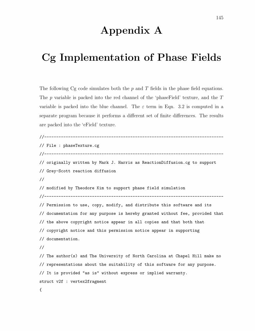
145

Appendix A

Cg Implementation of Phase Fields

The following Cg code simulates both the p and T fields in the phase field equations.

The p variable is packed into the red channel of the ‘phaseField’ texture, and the T

variable is packed into the blue channel. The ε term in Eqn. 3.2 is computed in a

separate program because it performs a different set of finite differences. The results

are packed into the ‘eField’ texture.

//---------------------------------------------------------------------------

// File : phaseTexture.cg

//---------------------------------------------------------------------------

// originally written by Mark J. Harris as ReactionDiffusion.cg to support

// Grey-Scott reaction diffusion

//

// modified by Theodore Kim to support phase field simulation

//---------------------------------------------------------------------------

// Permission to use, copy, modify, and distribute this software and its

// documentation for any purpose is hereby granted without fee, provided that

// the above copyright notice appear in all copies and that both that

// copyright notice and this permission notice appear in supporting

// documentation.

//

// The author(s) and The University of North Carolina at Chapel Hill make no

// representations about the suitability of this software for any purpose.

// It is provided "as is" without express or implied warranty.

struct v2f : vertex2fragment

{

146

float4 texCoord : TEX0;

};

fragout main(v2f IN,

// dimensions of the current window

uniform float4 windowDims,

// simulation parameters

uniform float4 iceParams,

// current timestep

uniform float timestep,

// texture containing the values of \varepsilon

uniform samplerRECT eField,

// texture containing the phase field variables

// the red channel is the phase variable $p$

// the blue channel is the heat variable $T$

uniform samplerRECT phaseField)

{

fragout OUT;

// get neighbors of current pixel

float4 rightPhase = f4texRECT(phaseField, IN.texCoord + fixed2(1,0));

float4 leftPhase = f4texRECT(phaseField, IN.texCoord + fixed2(-1,0));

float4 downPhase = f4texRECT(phaseField, IN.texCoord + fixed2(0,-1));

float4 upPhase = f4texRECT(phaseField, IN.texCoord + fixed2(0,1));

// get neighbors of \varepsilon term

147

float3 leftE = f3texRECT(eField, IN.texCoord + fixed2(-1,0));

float3 rightE = f3texRECT(eField, IN.texCoord + fixed2(1,0));

float3 downE = f3texRECT(eField, IN.texCoord + fixed2(0,-1));

float3 upE = f3texRECT(eField, IN.texCoord + fixed2(0,1));

// compute the off-diagonal partial derivatives

float pdydx = (rightE.z - leftE.z) * windowDims.z;

float pdxdy = (upE.y - downE.y) * windowDims.z;

// compute the on-diagonal partial derivatives (the Hessian)

float4 centerPhase = f4texRECT(phaseField, IN.texCoord);

float4 dx = (-2.0 * centerPhase + leftPhase + rightPhase) *

windowDims.w;

float4 dy = (-2.0 * centerPhase + upPhase + downPhase) *

windowDims.w;

float laplacian = f1texRECT(eField, IN.texCoord) * (dx.x + dy.x);

// compute the potential (the cubic reaction term)

float m = iceParams.x *

atan(iceParams.y * (centerPhase.z - centerPhase.y));

m = (centerPhase.z - centerPhase.y == 0.0f) ? 0.0f : m;

float potential = centerPhase.x * (1.0f - centerPhase.x) *

(centerPhase.x - 0.5f + m);

// compute the final $\frac{\partial p}{\partial t}$

float phaseDt = ((pdxdy - pdydx) + laplacian + potential) *

iceParams.z;

// timestep the $p$ field

OUT.col.r = centerPhase.x + phaseDt * timestep;

148

// timestep the $T$ field

OUT.col.g = centerPhase.y +

((dx.y + dy.y) + phaseDt * iceParams.w) * timestep;

OUT.col.b = centerPhase.z;

float ICE_expansion = 0.00025f;

OUT.col.a = (OUT.col.r > 0.5f) ? centerPhase.w + phaseDt * ICE_expansion :

centerPhase.w;

return OUT;

}

Because it performs a separate set of finite differences, the ε term in Eqn. 3.2 is

computed in the separate program, listed here.

//---------------------------------------------------------------------------

// File : eTexture.cg

//---------------------------------------------------------------------------

// originally written by Mark J. Harris as ReactionDiffusion.cg to support

// Grey-Scott reaction diffusion

//

// modified by Theodore Kim to support phase field simulation

//---------------------------------------------------------------------------

// Permission to use, copy, modify, distribute and sell this software and its

// documentation for any purpose is hereby granted without fee, provided that

// the above copyright notice appear in all copies and that both that

// copyright notice and this permission notice appear in supporting

// documentation.

//

// The author(s) and The University of North Carolina at Chapel Hill make no

// representations about the suitability of this software for any purpose.

// It is provided "as is" without express or implied warranty.

149

struct v2f : vertex2fragment

{

float4 texCoord : TEX0;

};

fragout main(v2f IN,

uniform samplerRECT phaseField,

uniform float4 windowDims,

uniform float4 iceParams)

{

fragout OUT;

// get neighboring pixels

float right = f1texRECT(phaseField, IN.texCoord + fixed2(1,0));

float left = f1texRECT(phaseField, IN.texCoord + fixed2(-1,0));

float down = f1texRECT(phaseField, IN.texCoord + fixed2(0,-1));

float up = f1texRECT(phaseField, IN.texCoord + fixed2(0,1));

// compute partial derivatives

float2 partial = float2((right - left), (up - down));

partial *= windowDims.z;

// compute a theta direction

float magnitude = length(partial);

float theta = (magnitude > 0.0f)

? acos(clamp(partial.x / magnitude, -1.0f, 1.0f))

: 0.0f;

theta = (partial.y < 0.0f) ? 2.0f * 3.1415926535897931f - theta

: theta;

// compute $\varepsilon$

150

float e = iceParams.x *

(1.0f + iceParams.y *

cos(iceParams.z * (theta - iceParams.w)));

float2 eedTheta = e * -iceParams.x * iceParams.z *

iceParams.y *

sin(iceParams.z * (theta - iceParams.w));

eedTheta *= partial;

// store various forms of $\varepsilon$

OUT.col.r = e * e;

OUT.col.g = eedTheta.x;

OUT.col.b = eedTheta.y;

return OUT;

}

151

Bibliography

Adalsteinsson, D. and Sethian, J. (1995a). A fast level set method for propagating

interfaces. Journal of Computational Physics, 118:pp. 269–277.

Adalsteinsson, D. and Sethian, J. (1995b). A level set approach to a unified model for

etching, deposition, and lithography, i: Two-dimensional simulations. J. Comp,

Phys., 120(1):128–144.

Adalsteinsson, D. and Sethian, J. (1995c). A level set approach to a unified model for

etching, deposition, and lithography, ii: Three-dimensional simulations. J. Comp,

Phys., 122(2):348–366.

Adalsteinsson, D. and Sethian, J. (1997). A level set approach to a unified model

for etching, deposition, and lithography, iii: Re-deposition, re-emission, surface

diffusion, and complex simulations. J. Comp, Phys., 138(1):193–223.

Adalsteinsson, D. and Sethian, J. (1999). The fast construction of extension velocities

in level set methods. Journal of Computational Physics, pages 2–22.

Al-Rawahi, N. and Tryggvason, G. (2002). Numerical simulation of dendritic solidi-

fication with convection: Two-dimensional geometry. Journal of Computational

Physics, 180:471–496.

Anderson, D., McFadden, G., and Wheeler, A. (2000). A phase-field model of solidifi-

cation with convection. Physica D, 135:175–194.

Atkinson, K. (1989). An Introduction to Numerical Analysis. John Wiley & Sons.

152

Ball, R. and Brady, R. (1985). Large scale lattice effect in diffusion-limited aggregation.

J. Phys. A: Math. Gen., 18:L809–L813.

Baxter, W. V., Wendt, J., and Lin, M. C. (2004). IMPaSTo: A realistic model for

paint. In Proceedings of the 3rd International Symposium on Non-Photorealistic

Animation and Rendering, pages 45–56.

Beckermann, C., Diepers, H., Steinbach, I., Karma, A., and Tong, X. (1999). Modeling

melt convection in phase-field simulations of solidification. Journal of Computa-

tional Physics, 154:468–496.

Ben-Jacob, E., Goldenfeld, N., Langer, J. S., and Schon, G. (1983). Dynamics of

interfacial pattern formation. Physical Review Letters, 51:19301932.

Ben-Jacob, E., Goldenfeld, N., Langer, J. S., and Schon, G. (1984). Boundary-layer

model of pattern formation in solidification. Physical Review A, 29:330–340.

Benney, D. (1966). Long waves on liquid films. Journal of Mathematical Physics,

45:150.

Bentley, W. (1902). Noaa photo library. http://www.photolib.noaa.gov/historic/nws/

nwind27.htm.

Bentley, W. and Humphreys, W. (1962). Snow Crystals. Dover Publications.

Bodenschatz, E., Imbihl, R., and Rehberg, I. (2003). Focus on pattern formation. New

Journal of Physics, 5.

Bogoyavlenskiy, V. A. (2001). Mean-field diffusion-limited aggregation: A density

model for viscous fingering phenomena. Physical Review E, 64:066303.

Bolz, J., Farmer, I., Grinspun, E., and Schroder, P. (2003). Sparse matrix solvers on

the gpu: Conjugate gradients and multigrid. Proc. of ACM SIGGRAPH.

Brener, E. and Mel‘nikov, V. (1991). 2-dimensional dendritic growth at arbitrary peclet

number. Adv. Phys.

153

Buka, A., Borzsonyi, T., Eber, N., and Toth-Katona, T. (2001). Patterns in the bulk

at the interface of liquid crystals. Lecture Notes in Physics, pages 298–318.

Caginalp, G. and Chen, X. (1992). Phase field equations in the sinulgar limit of sharp

interface problems. In Gurtin, M. and McFadden, G., editors, On the Evolution

of Phase Boundaries, volume 43, pages 1–27. Springer Verlag.

Canny, J. (1986). A computational approach to edge detection. IEEE Transactions on

Pattern Analysis and Machine Intelligence, 8(6):pp. 679–698.

Carlson, M., Mucha, P., III, B. V. H., and Turk, G. (2002). Melting and flowing. Proc.

of ACM SIGGRAPH Symposium on Computer Animation.

Carlson, M., Mucha, P. J., and Turk, G. (2004). Rigid fluid: animating the interplay

between rigid bodies and fluid. ACM Trans. Graph., 23(3):377–384.

Chen, S., Merriman, B., Osher, S., and Smereka, P. (1997). A simple level set method

for solving stefan problems. Journal of Computational Physics, 135:8–29.

Chen, Y., Xia, L., Wong, T.-T., Tong, X., Bao, H., Guo, B., and Shum, H.-Y. (2005).

Visual simulation of weathering by gamma-ton tracing. ACM Trans. Graph.,

24(3).

Chopp, D. (2001). Some improvements of the fast marching method. Journal of Sci-

entific Computing, 23:230–244.

Clavet, S., Beaudoin, P., and Poulin, P. (2005). Particle-based viscoelastic fluid simu-

lation. In Symposium on Computer Animation 2005, pages 219–228.

Cook, R. and Torrance, K. (1982). A reflectance model for computer graphics. ACM

Transactions on Graphics, 1:7–24.

Demmel, J. (1997). Applied Numerical Linear Algebra. SIAM.

DeRose, T., Kass, M., and Troung, T. (1998). Subdivision surfaces in character ani-

mation. Proc. of ACM SIGGRAPH.

154

Desbenoit, B., Galin, E., and Akkouche, S. (2004). Simulating and modeling lichen

growth. Proc. of Eurographics 2004.

Donner, C. and Jensen, H. W. (2005). Light diffusion in multi-layered translucent

materials. ACM Trans. Graph., 24(3).

Dorsey, J. and Hanrahan, P. (1996). Modeling and rendering of metallic patinas. Proc.

of SIGGRAPH, pages 378–396.

Dorsey, J., Pedersen, H. K., and Hanrahan, P. (1996). Flow and changes in appear-

ance. In SIGGRAPH ’96: Proceedings of the 23rd annual conference on Computer

graphics and interactive techniques, pages 411–420.

Eden, M. (1961). A two dimensional growth process. In Proceedings of the Fourth

Berkeley Symposium on Mathematical Statistics and Probability.

Enright, D., Fedkiw, R., Ferziger, J., and Mitchell, I. (2002a). A hybrid particle level

set method for improved interface capturing. Journal of Computational Physics,

183:83–116.

Enright, D., Marschner, S., and Fedkiw, R. (2002b). Animation and rendering of

complex water surfaces. Proc. of SIGGRAPH, pages pp. 736–744.

Family, F., Platt, D. E., and Vicsek, T. (1987). Deterministic growth model of pattern

formation in dendritic solidification. Journal of Physics A, 20:L1177–L1183.

Fearing, P. (2000). Computer modeling of fallen snow. Proc. of SIGGRAPH, pages

37–46.

Fedkiw, R., Stam, J., and Jensen, H. W. (2001). Visual simulation of smoke. Proc. of

SIGGRAPH, pages 15–22.

Feldman, B. E., O’Brien, J. F., and Klingner, B. M. (2005). Animating gases with

hybrid meshes. In Proceedings of ACM SIGGRAPH 2005.

155

Fix, G. (1983). Free boundary problems, theory and applications. In Fasans, A. and

Primicero, M., editors, Research Notes In Mathematics, volume 2. Pitman.

Foster, N. and Fedkiw, R. (2001). Practical animation of liquids. Proc. of SIGGRAPH,

pages pp. 15–22.

Foster, N. and Metaxas, D. (1996). Realistic animation of liquids. In Proceedings GI

’96, pages 204–212.

Frank, F. (1949). The influence of dislocation on crystal growth. Disc. Faraday Soc.,

5:48–54.

Frank, F. C. (1974). Descartes’ observations on the amsterdam snowfalls of 4, 5, 6 and

9 february 1634. Journal of Glaciology, 13(69):535–539.

Galoppo, N., Govindaraju, N., Henson, M., and Manocha, D. (2005). Lu-gpu: Efficient

algorithms for solving dense linear systems on graphics hardware. In Proceedings

of the ACM/IEEE SC—05 Conference.

Gibou, F. and Fedkiw, R. (2005). A fourth order accurate discretization for the laplace

and heat equations on arbitrary domains, with applications to the stefan problem.

J. Comput. Phys., 202:577–601.

Gibou, F., Fedkiw, R., Caflisch, R., and Osher, S. (2003). A level set approach for the

simulation of dendritic growth. J. Sci. Comput., 19:183–199.

Goktekin, T. G., Bargteil, A. W., and O’Brien, J. F. (2004). A method for animating

viscoelastic fluids. ACM Transactions on Graphics (Proc. of ACM SIGGRAPH

2004), 23(3):463–468.

Goldsworthy, A. (1990). Andy Goldsworthy: A Collaboration with Nature. Harry N

Abrams.

156

Govindaraju, N., Redon, S., Lin, M., and Manocha, D. (2003). Cullide: Interactive

collision detection between complex models in large environments using graphics

hardware. ACM SIGGRAPH/Eurographics Graphics Hardware.

Griebel, M., Dornseifer, T., and Neunhoeffer, T. (1997). Numerical Simulation in Fluid

Dynamics: A Practical Introduction. SIAM.

Haji-Sheikh, A. (1988). Monte carlo methods. In Minkowycz, W., Sparrow, E., Schnei-

der, G., , and Pletcher, R., editors, Handbook of Numerical Heat Transfer, pages

673–723. John Wiley and Sons.

Halperin, B., Hohenberg, P., and Ma, S. (1974). Renormalization group methods for

critical dynamics. Physical Review B, 10:139–153.

Harlow, F. and Welch, E. (1966). Numerical calculation of time-dependent viscous

incompressible flow of fluids with free surface. Physics of Fluids, 8.

Harris, M. J., Coombe, G., Scheuermann, T., and Lastra, A. (2002). Physically-based

visual simulation on graphics hardware. Proc. 2002 SIGGRAPH / Eurographics

Workshop on Graphics Hardware.

Harten, A., Engquist, B., Osher, S., and Chakravarthy, S. (1987). Uniformly high-

order accurate essentially non-oscillatory schemes iii. Journal of Computational

Physics, 71:231–303.

Hastings, M. (2001). Fractal to nonfractal phase transition in the dielectric breakdown

model. Physical Review Letters, 87(17).

Hastings, M. and Levitov, L. (1998). Laplacian growth as one-dimensional turbulence.

Physica D, 116:244–252.

Hill, J. M. (1987). One-dimensional Stefan Problems: an Introduction. John Wiley &

Sons.

Hooke, R. (1665). Micrographia. Dover Publications.

157

Hoppe, H. (1994). Surface reconstruction from unorganized points. PhD thesis, Uni-

versity of Washington.

Ivantsov, G. (1947). Temperature field around the spherical, cylindrical and needle-

crystals which grow in supercooled melt. Dokl Akad Nauk USSR, 58:67.

Jahne, B. (1997). Digital Image Processing: Concepts, Algorithms, and Scientific Ap-

plications. Springer Verlag.

Jensen, H. (2001). Realistic Image Synthesis Using Photon Mapping. AK Peters.

Jensen, H., Legakis, J., and Dorsey, J. (1999). Rendering of wet materials. Rendering

Techniques ’99, pages 273–282.

Jensen, H., Marschner, S., Levoy, M., and Hanrahan, P. (2001a). A practical model for

subsurface light transport. Proceedings of SIGGRAPH 2001.

Jensen, H., Marschner, S., Levoy, M., and Hanrahan, P. (2001b). A practical model for

subsurface light transport. Proceedings of SIGGRAPH 2001, pages 511–518.

Jones, M. and Chen, M. (1994). A new approach to the construction of surfaces from

contour data. Computer Graphics Forum, 13(3):pp. 75–84.

Jou, D., Casas-Vazquez, J., and Criado-Sancho, M. (2001). Thermodynamics of Fluids

Under Flow. Springer-Verlag.

Kass, M. and Miller, G. (1990). Rapid, stable fluid dynamics for computer graphics.

In Proceedings of SIGGRAPH 1990, pages 49–57.

Kaufman, H., Vespignani, A., Mandelbrot, B., and Woog, L. (1995). Parallel diffusion-

limited aggregation. Physical Review E, 52:5602–5609.

Kepler, J. (1611). The Six-Cornered Snowflake. Oxford Univ. Press. Translated by L.

L. Whyte, 1966.

158

Kharitonsky, D. and Gonczarowski, J. (1993). A physically based model for icicle

growth. The Visual Computer, pages 88–100.

Kim, T. and Lin, M. (2003). Visual simulation of ice crystal growth. Proc. of ACM

SIGGRAPH / Eurographics Symposium on Computer Animcation.

Kim, T. and Lin, M. (2004). Physically based modeling and rendering of lightning.

Proc. of Pacific Graphics 2004.

Kobayashi, R. (1993). Modeling and numerical simulations of dendritic crystal growth.

Physica D, 63:pp. 410–423.

Landis, H. (2002). Production-ready global illumination. In Siggraph course notes #16.

Langer, J. S. (1986). Models of pattern formation in first-order phase transitions. In

Grinstein, G. and Mazenko, G., editors, Directions in Condensed Matter Physics,

pages 165–186. World Scientific.

Langer, M. S., Zhang, L., Klein, A., Bhatia, A., Pereira, J., and Rekhi, D. (2004). A

spectral-particle hybrid method for rendering falling snow. In Rendering Tech-

niques 2004: Eurographics Symposium on Rendering, pages 217–226.

Liu, X., Osher, S., and Chan, T. (1996). Weighted essentially non-oscillatory schemes.

Journal of Computational Physics, 126:202–212.

Losasso, F., Gibou, F., and Fedkiw, R. (2004). Simulating water and smoke with an

octree data structure. Proc. of SIGGRAPH, pages 457–462.

Losasso, F., Irving, G., Guendelman, E., and Fedkiw, R. (2005). Melting and burning

solids into liquids and solids. IEEE TVCG.

Maeno, N., Makkonen, L., Nishimura, K., Kosugi, K., and Takahashi, T. (1994).

Growth rates of icicles. Journal of Glaciology, 40:319–326.

Makkonen, L. (1988). A model of icicle growth. Journal of Glaciology, pages 64–70.

159

Malladi, R., Sethian, J., and Vemuri, B. (1995). Shape modeling with front propagation:

A level set approach. IEEE Trans. on Pattern Analysis and Machine Intelligence,

17(2).

Mandelbrot, B. (1982). The Fractal Geometry of Nature. W H Freeman.

Mandelbrot, B. and Evertsz, C. (1990). The potential distribution around growing

fractal clusters. Nature, 348:L143–L145.

McNamara, A., Treuille, A., Popovic, Z., and Stam, J. (2004). Fluid control using the

adjoint method. ACM Transactions on Graphics, 23(3):449–456.

Meakin, P. (1983). Diffusion-controlled cluster formation in two, three, and four di-

mensions. Physical Review A, 27:604–607.

Meirmanov, A. (1992). The Stefan problem. W. De Gruyter expositions in mathematics.

Messinger, B. (1953). Equilibrium temperature of an unheated icing surface as a func-

tion of air speed. J. Aero. Sci, pages 29–42.

Mullins, W. and Sekerka, R. (1964). Stability of a planar interface during solidification

of a dilute binary alloy. Journal of Applied Physics, 35(2):444–451.

Myers, T. and Hammond, D. (1999). Ice and water film growth from incoming super-

cooled droplets. International Journal of Heat and Mass Transfer, 42:PP2233–

2242.

Nagatani, T. and Sagues, F. (1991). Morphological changes in convection-diffusion-

limited deposition. Physical Review A, 43:2970–2976.

Nakaya, U. (1954). Snow Crystals, Natural and Artificial. Harvard University Press.

Niemeyer, L., Pietronero, L., and Wiesmann, H. J. (1984). Fractal dimension of dielec-

tric breakdown. Physical Review Letters, 52:1033–1036.

160

Nishita, T., Iwasaki, H., Dobashi, Y., and Nakamae, E. (1997). A modeling and render-

ing method for snow by using metaballs. Computer Graphics Forum, 16(3):357–

364.

Nittmann, J. and Stanley, H. E. (1987). Non-deterministic approach to anisotropic

growth patterns with continuously tunable morphology: the fractal properties of

some real snowflakes. Journal of Physics A, 20:L1185–L1191.

Ogawa, N. and Furukawa, Y. (2002). Surface instability of icicles. Physical Review E,

66:041202.

Osher, S. and Fedkiw, R. (2003). Level Set Methods and Dynamic Implicit Surfaces.

Springer Verlag.

Osher, S. and Sethian, J. (1988). Fronts propagating with curvature-dependent speed:

Algorithms based on hamilton–jacobi formulations. Journal of Computational

Physics, 79:12–49.

Plapp, M. and Karma, A. (2000). Multiscale finite-difference-diffusion-monte-carlo

method for simulating dendritic solidification. Journal of Computational Physics,

p. 165:592–619.

Provatas, N., Goldenfeld, N., and Dantzig, J. (1999). Adaptive mesh refinement com-

putation of solidification microstructures using dynamic data structures. Journal

of Computational Physics, 148:p. 265.

Rasmussen, N., Enright, D., Nguyen, D., Marino, S., Sumner, N., Geiger, W., Hoon, S.,

and Fedkiw, R. (2004). Directable photorealistic liquids. In SCA ’04: Proceedings

of the 2004 ACM SIGGRAPH/Eurographics symposium on Computer animation,

pages 193–202.

Rebelo, L., Debenedetti, P., and Sastry, S. (1998). Singularity-free interpretation of the

thermodynamics of supercooled water ii. Journal of Chemical Physics, 109(2):pp.

626–633.

161

Roberts, A. and Knackstedt, M. (1993). Growth in non-laplacian fields. Physical Review

E, 47:2724–2728.

Runions, A., Fuhrer, M., Lane, B., Federl, P., Rolland-Lagan, A., and Prusinkiewicz,

P. (2005). Modeling and visualization of leaf venation patterns. ACM Trans.

Graph., 24:702–711.

Saad, Y. (2003). Iterative Methods For Sparse Linear Systems. SIAM.

Saffman, P. and Taylor, G. (1958). The penetration of a fluid into a porous medium or

hele-shaw cell containing a more viscous liquid. Proceedings of the Royal Society

of London, Serial A, 245:312–329.

Saito, Y. (1996). Statistical Physics of Crystal Growth. World Scientific.

Sander, L. (2000). Diffusion limited aggregation: A kinetic critical phenomenon? Con-

temporary Physics, 41(4):203–218.

Selle, A., Rasmussen, N., and Fedkiw, R. (2005). A vortex particle method for smoke,

water and explosions. In Proceedings of ACM SIGGRAPH 2005, pages 910–914.

Sethian, J. (1999). Level Set Methods and Fast Marching Methods. Cambridge Univer-

sity Press.

Sethian, J. and Strain, J. (1992). Crystal growth and dendritic solidification. J. Comput.

Phys., 98:231–253.

Shewchuk, J. R. (1994). An introduction to the conjugate gradient method without

the agonizing pain. Technical report, Carnegie Mellon University.

Shewchuk, J. R. (1996). Triangle: Engineering a 2D Quality Mesh Generator and

Delaunay Triangulator. In Lin, M. C. and Manocha, D., editors, Applied Com-

putational Geometry: Towards Geometric Engineering, volume 1148 of Lecture

Notes in Computer Science, pages 203–222. Springer-Verlag. From the First ACM

Workshop on Applied Computational Geometry.

162

Short, M. B., Baygents, J. C., Beck, J. W., Stone, D. A., III, R. S. T., and Goldstein,

R. E. (2005). Stalactite growth as a free-boundary problem: A geometric law and

its platonic ideal. Physical Review Letters, 94(1):018501.

Stam, J. (1999a). Diffraction shaders. In SIGGRAPH ’99: Proceedings of the 26th

annual conference on Computer graphics and interactive techniques, pages 101–

110.

Stam, J. (1999b). Stable fluids. Proc. of SIGGRAPH, pages 121–128.

Stefan, J. (1889). Uber einige probleme der theorie der warmeleitung. Sitzungsberichte

de Mathematisch- Naturawissenschaftlichen Classe der Kaiserlichen, Akademie

der Wissenschaften, 98:473–84.

Sud, A., Otaduy, M. A., and Manocha, D. (2004). Difi: Fast 3d distance field compu-

tation using graphics hardware. 23.

Sumner, R. (2001). Pattern formation in lichen. Master’s thesis, Massachusetts Institute

of Technology.

Szilder, K. and Lozowski, E. (1994). An analytical model of icicle growth. Annals of

Glaciology, 19:141–145.

Touissaint, J.-C., Debierre, J.-M., and c Turban, L. (1992). Deposition of particles in

a two-dimensional lattice gas flow. Physical Review Letters, 68:2027–2030.

Trefethen, L. and Bau, D. (1997). Numerical Linear Algebra. SIAM.

Turing, A. (1952). The chemical basis of morphogenesis. Philosophical Transactions of

the Royal Society B, 237:37–72.

Turk, G. (1991). Generating textures on arbitrary surfaces using reaction-diffusion.

Proc. of SIGGRAPH, pages 289–298.

Ueno, K. (2003). Pattern formation in crystal growth under parabolic shear flow.

Physical Review E, 68:021603.

163

Ueno, K. (2004). Pattern formation in crystal growth under parabolic shear flow ii.

Physical Review E, 69:051604.

Vicsek, T. (1984). Pattern formation in diffusion-limited aggregation. Physical Review

Letters, 53:2281–2284.

von Koch, H. (1906). Une methode geometrique elementaire pour l’etude de certaines

questions de la theorie des courbes planes. Acta Mathematica, 30:pp. 145–174.

Wei, X., Li, W., and Kaufman, A. (2003). Interactive melting and flowing of viscous

volumes. Proceedings of Computer Animation and Social Agents 2003.

Wettlaufer, J. (2001). The Stefan Problem: Polar Exploration and the mathematics of

moving boundaries. Styria Verlag.

Witkin, A. and Kass, M. (1991). Reaction-diffusion textures. Proc. of SIGGRAPH,

pages pp. 299–308.

Witten, T. and Sander, L. (1981). Diffusion-limited aggregation, a kinetic critical

phenomenon. Physical Review Letters, 47(19):pp. 1400–1403.

Wong, T.-T., Luk, W.-S., and Heng, P.-A. (1997). Sampling with hammersley and

halton points. Journal of Graphics Tools.

Yokoyama, E. and Kuroda, T. (1990). Pattern formation in growth of snow crystals

occurring in the surface kinetic process and the diffusion process. Physical Review

A, page p. 41.