Reliable Computation of Phase Stability Using Interval Analysis:

Cubic Equation of State Models

James Z. HuaDepartment of Chemical Engineering

University of Illinois at Urbana-ChampaignUrbana, IL 61801 USA

Joan F. Brenneckeand

Mark A. Stadtherr�

Department of Chemical EngineeringUniversity of Notre DameNotre Dame, IN 46556 USA

April 1997(revised, October 1997)

Originally presented at6th European Symposium on Computer-Aided Process Engineering (ESCAPE-6),

Rhodes, Greece, May 26-29, 1996

�Author to whom all correspondence should be addressed. Fax: (219) 631-8366; E-mail: markst@nd.edu

Abstract

The reliable prediction of phase stability is a challenging computational problem in chemical

process simulation, optimization and design. The phase stability problem can be formulated either

as a minimization problem or as an equivalent nonlinear equation solving problem. Conventional

solution methods are initialization dependent, and may fail by converging to trivial or non-physical

solutions or to a point that is a local but not global minimum. Thus there has been consider-

able recent interest in developing more reliable techniques for stability analysis. In this paper we

demonstrate, using cubic equation of state models, a technique that can solve the phase stability

problem with complete reliability. The technique, which is based on interval analysis, is initializa-

tion independent, and if properly implemented provides a mathematical guarantee that the correct

solution to the phase stability problem has been found.

1 Introduction

The determination of phase stability, i.e., whether or not a given mixture can split into multiple

phases, is a key step in phase equilibrium calculations, and thus in the simulation and design of a

wide variety of processes, especially those involving separation operations such as distillation and

extraction. The phase stability problem is frequently formulated in terms of the tangent plane

condition (Baker et al., 1982). Minima in the tangent plane distance are sought, usually by solving

a system of nonlinear equations for the stationary points (Michelsen, 1982). If any of these yield

a negative tangent plane distance, indicating that the tangent plane intersects (or lies above) the

Gibbs energy of mixing surface, the phase is unstable and can split (in this context, unstable refers

to both the metastable and classically unstable cases). The di�culty lies in that, in general, given

any arbitrary equation of state or activity coe�cient model, most computational methods cannot

�nd with complete certainty all the stationary points, and thus there is no guarantee that the phase

stability problem has been correctly solved.

Standard methods (e.g., Michelsen, 1982) for solving the phase stability problem typically rely

on the use of multiple initial guesses, carefully chosen in an attempt to locate all stationary points

in the tangent plane distance function. However, these methods o�er no guarantee that the global

minimum in the tangent plane distance has been found. Because of the di�culties that thus

arise, there has been signi�cant recent interest in the development of more reliable methods for

solving the phase stability problem (e.g., Nagarajan et al., 1991; Sun and Seider, 1995; Eubank et

al., 1992; Wasylkiewicz et al., 1996; McDonald and Floudas, 1995a,b,c,1997). For example, Sun

and Seider (1995) apply a homotopy-continuation method, which will often �nd all the stationary

points, and is easier to initialize than Michelsen's approach. However, their technique is still

1

initialization dependent and provides no theoretical guarantees that all stationary points have

been found. The \area" method of Eubank et al. (1992), which is based on exhaustive search

over a grid, can also be very reliable. They suggest that a course grid be used �rst to �nd the

approximate location of solutions. Then, regions appearing not to contain a solution are arbitrarily

eliminated from consideration and the search continues with a �ner grid in the remaining regions.

However, there is no mathematical guarantee provided that the regions eliminated do not contain

solutions. McDonald and Floudas (1995a,b,c,1997) show that for certain activity coe�cient models,

the phase stability problem can be reformulated to make it amenable to solution by powerful global

optimization techniques, which do guarantee that the correct answer is found. However, in general

there appears to remain a need for an e�cient general-purpose method that can perform phase

stability calculations with mathematical certainty for any arbitrary equation of state (EOS) or

activity coe�cient model.

An alternative approach, based on interval analysis, that satis�es these needs was originally

suggested by Stadtherr et al. (1995), who applied it in connection with activity coe�cient models,

as later done also by McKinnon et al. (1996). This technique, in particular the use of an interval

Newton/generalized bisection algorithm, is initialization independent and can solve the phase sta-

bility problem with mathematical certainty. Recently Hua et al. (1996a) extended this method to

problems modeled using a simple cubic EOS (Van der Waals equation). In this paper we seek to

extend the application of this technique to cubic EOS models in general. Though the technique

developed is general-purpose, the applications presented focus on the Peng-Robinson (PR) and

Soave-Redlich-Kwong (SRK) models with standard mixing rules.

2

2 Phase Stability Analysis

The determination of phase stability is often done using tangent plane analysis (Baker et al.,

1982; Michelsen, 1982). A phase at speci�ed T , P , and feed mole fraction z is unstable if the molar

Gibbs energy of mixing surface m(x; v) = �gmix = �Gmix=RT ever falls below a plane tangent to

the surface at z. That is, if the tangent plane distance

D(x; v) = m(x; v) �m0 �nXi=1

�@m

@xi

�0(xi � zi) (1)

is negative for any composition x, the phase is unstable. The subscript zero indicates evaluation

at x = z, n is the number of components, and v is the molar volume of the mixture. A common

approach for determining if D is ever negative is to minimize D subject to the mole fractions

summing to one and subject to the equation of state relating x and v. It is readily shown that

the stationary points in this optimization problem can be found by solving the system of nonlinear

equations:��

@m

@xi

���@m

@xn

�����

@m

@xi

���@m

@xn

��0= 0; i = 1; : : : ; n� 1 (2)

1�nXi=1

xi = 0 (3)

P � RT

v � b+

a

v2 + ubv + wb2= 0 (4)

Equation (4) is the generalized cubic EOS given by Reid et al. (1987). With the appropriate choice

of u and w, common models such as PR (u = 2, w = �1) and SRK (u = 1, w = 0) may be obtained.

For all the example problems considered here, standard mixing rules, namely b =Pn

i=1 xibi and

a =Pn

i=1

Pnj=1 xixjaij , are used, with aij = (1�kij)paiiajj. The aii(T ) and bi are pure component

properties determined from the system temperature T , the critical temperatures Tci, the critical

pressures Pci and acentric factors !i.

3

For this EOS the reduced molar Gibbs energy of mixing is given by:

m(x; v) =Pv

RT+ ln

�RT

v � b

�+

a

RTb�ln

�2v + ub� b�

2v + ub+ b�

�+

nXi=1

xi lnxi �nXi=1

xigoi (5)

where the goi represent the pure component reduced molar Gibbs energies and � =pu2 � 4w.

Substituting into equation (2) yields

si(x; v) � si(z; v0) = 0 i = 1; : : : ; n� 1 (6)

where

si =@m

@xi� @m

@xn

=bi � bn

b

�Pv

RT� 1

�+

a

bRT�

�2(�ai � �an)

a� bi � bn

b

�ln

�2v + ub� b�

2v + ub+ b�

�

+ lnxixn

� (goi � gon)

and �ai =Pn

k=1 xkaik. If there are multiple real volume roots at the feed composition, then in

equation (6) the molar volume v0 at the feed composition must be the root yielding the minimum

value of m(z; v0), the reduced molar Gibbs energy of mixing at the feed.

The (n + 1) � (n + 1) system given by equations (3), (4) and (6) above has a trivial root at

x = z and v = v0 and frequently has multiple nontrivial roots as well. Thus conventional equation

solving techniques may fail by converging to the trivial root or give an incorrect answer to the phase

stability problem by converging to a stationary point that is not the global minimum of D. This

is aptly demonstrated by the experiments of Green et al. (1993), who show that the pattern of

convergence from di�erent initial guesses demonstrates a complex fractal-like behavior for even very

simple models. We demonstrate here the use of an interval Newton/generalized bisection method

for solving the system of equations (3), (4) and (6). The method requires no initial guess, and will

�nd with certainty all the stationary points of the tangent plane distance D.

4

3 Interval Computations

A real interval, X, is de�ned as the continuum of real numbers lying between (and including)

given upper and lower bounds; i.e., X = [a; b] = fx 2 < j a � x � bg, where a; b 2 < and a � b.

A real interval vector X = (X1;X2; :::;Xn)T has n real interval components and since it can be

interpreted geometrically as an n-dimensional rectangle, is frequently referred to as a box. Note

that in this section lower case quantities are real numbers and upper case quantities are intervals.

Several good introductions to computation with intervals are available, including monographs by

Neumaier (1990), Hansen (1992), and Kearfott (1996).

Of particular interest here are interval Newton/generalized bisection (IN/GB) methods. These

techniques provide the power to �nd with con�dence all solutions of a system of nonlinear equations

(Neumaier, 1990; Kearfott and Novoa, 1990), and to �nd with total reliability the global minimum

of a nonlinear objective function (Hansen, 1992), provided only that upper and lower bounds are

available for all variables. E�cient techniques for implementing IN/GB are a relatively recent

development, and thus such methods have not yet been widely applied. Schnepper and Stadtherr

(1990) have suggested the use of this method for solving chemical process modeling problems, and

recently described an implementation (Schnepper and Stadtherr, 1996). Balaji and Seader (1995)

have also successfully applied the method to chemical engineering problems.

Consider the solution of the system of real nonlinear equations f(x) = 0, where it is desired to

�nd all solutions in an speci�ed initial interval X(0). The basic iteration step in interval Newton

methods is, given an interval X(k), to solve the linear interval equation system

F 0(X(k))(N(k) � x(k)) = �f(x(k)) (7)

for a new interval N(k), where k is an iteration counter, F 0(X(k)) is an interval extension of the

5

real Jacobian f 0(x) of f(x) over the current interval X(k), and x(k) is a point in the interior of

X(k), usually taken to be the midpoint. One way to evaluate the interval extension F 0(X(k)) of the

Jacobian is to substitute the interval X(k) for x in the expression f 0(x) for the real Jacobian, and

perform interval operations in place of real operations. It can be shown (Moore, 1966) that any

root x� of the set of equations that is within the current interval, i.e. x� 2 X(k), is also contained

in the newly computed interval N(k). This suggests that the next iteration for X should be the

intersection of X(k) with N(k), i.e. X(k+1) = X(k) \ N(k). There are various interval Newton

methods, which di�er in how they determine N(k) from equation (7) and thus in the tightness with

which N(k) encloses the solution set of (7).

While the iteration scheme discussed above can be used to tightly enclose a solution, what is

of most signi�cance here is the power of equation (7) to provide a test of whether a solution exists

within a given interval and whether it is a unique solution. For several techniques for �nding N(k)

from equation (7), it can be proven (e.g., Neumaier, 1990) that if N(k) is totally contained within

X(k), i.e. N(k) � X(k), then there is a unique zero of the set of nonlinear equations f(x) = 0 in

X(k), and furthermore that Newton's method with real arithmetic will converge to that solution

starting from any point in X(k). Thus, if N(k) is determined using one of these techniques, the

computation can be used as a root inclusion test for any interval X(k):

1. If X(k) and N(k) do not intersect, i.e., X(k) \ N(k) = ;, then there is no root in X(k).

2. If N(k) is totally contained in X(k), then there is exactly one root in X(k) and Newton's

method with real arithmetic will �nd it.

3. If neither of the above is true, then no conclusion can be drawn.

In the last case, one could then repeat the root inclusion test on the next interval Newton iterate

6

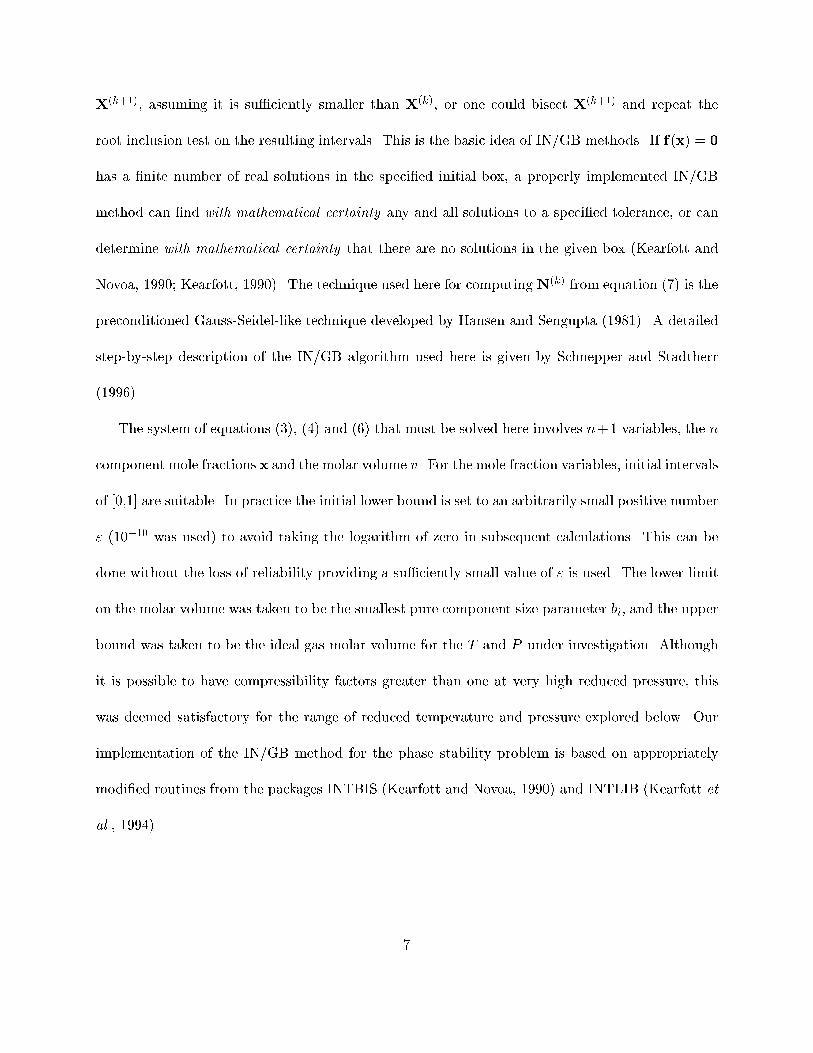
X(k+1), assuming it is su�ciently smaller than X(k), or one could bisect X(k+1) and repeat the

root inclusion test on the resulting intervals. This is the basic idea of IN/GB methods. If f(x) = 0

has a �nite number of real solutions in the speci�ed initial box, a properly implemented IN/GB

method can �nd with mathematical certainty any and all solutions to a speci�ed tolerance, or can

determine with mathematical certainty that there are no solutions in the given box (Kearfott and

Novoa, 1990; Kearfott, 1990). The technique used here for computing N(k) from equation (7) is the

preconditioned Gauss-Seidel-like technique developed by Hansen and Sengupta (1981). A detailed

step-by-step description of the IN/GB algorithm used here is given by Schnepper and Stadtherr

(1996).

The system of equations (3), (4) and (6) that must be solved here involves n+1 variables, the n

component mole fractions x and the molar volume v. For the mole fraction variables, initial intervals

of [0,1] are suitable. In practice the initial lower bound is set to an arbitrarily small positive number

" (10�10 was used) to avoid taking the logarithm of zero in subsequent calculations. This can be

done without the loss of reliability providing a su�ciently small value of " is used. The lower limit

on the molar volume was taken to be the smallest pure component size parameter bi, and the upper

bound was taken to be the ideal gas molar volume for the T and P under investigation. Although

it is possible to have compressibility factors greater than one at very high reduced pressure, this

was deemed satisfactory for the range of reduced temperature and pressure explored below. Our

implementation of the IN/GB method for the phase stability problem is based on appropriately

modi�ed routines from the packages INTBIS (Kearfott and Novoa, 1990) and INTLIB (Kearfott et

al., 1994).

7

4 Results

To test this initial implementation of IN/GB to solve phase stability problems for cubic equations

of state, several di�erent mixtures have been used. Results for mixtures modeled using either the

SRK or PR EOS are presented here. In order to demonstrate the power of the method, in these

studies we have found all the stationary points. However, it should be emphasized that, for making

a determination of phase stability or instability, �nding all the stationary points is not always

necessary, as discussed in more detail below.

4.1 Problem 1

This is a mixture of hydrogen sul�de (1) and methane (2) at 190 K and 40.53 bar (40 atm.).

The SRK model was used with parameters calculated from Tc1 = 373.2 K, Pc1 = 89.4 bar, !1 =

0.1, Tc2 = 190.6 K, Pc2 = 46.0 bar, !2 = 0.008, and a binary interaction parameter k12 = 0.08. A

plot of the reduced Gibbs energy of mixing m vs. x1 for this system is shown in Figure 1.

Several feeds were considered, as shown in Table 1, which also shows the roots (stationary

points) found, and the value of the tangent plane distance D at each root. For the z1 = 0.5 case,

our results are consistent with those given by Sun and Seider (1995) for this problem. For the z1

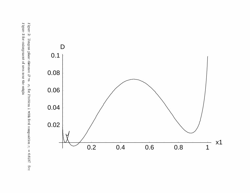
= 0.0187 case, a plot of the tangent plane distance D vs. x1 is shown in Figures 2 and 3. For feeds

near this point, this is known to be a di�cult problem to solve (e.g., Michelsen, 1982; Sun and

Seider, 1995). As noted by Michelsen and others, if one uses a locally convergent solver, with nearly

pure CH4 as the initial guess, convergence will likely be to the trivial solution at x1 = z1 = 0:0187.

And if nearly pure H2S is the initial guess, convergence will likely be to the local, but not global,

minimum at x1 = 0:8848. Using only these initial guesses would lead to the incorrect conclusion

8

that the mixture is stable. This is indicative of the importance of the initialization strategy when

conventional methods are used. An important advantage of the IN/GB approach described here is

that it eliminates the initialization problem, since it is initialization independent. In this case, it

�nds all the stationary points, including the global minimum at x1 = 0:0767, correctly predicting,

since D < 0 at this point, that a mixture with this feed composition is unstable. Michelsen's

algorithm, as implemented in LNGFLASH from the IVC-SEP package (Hytoft and Gani, 1996), a

code that in general we have found to be extremely reliable, incorrectly predicts that this mixture

is stable. As indicated in Table 1, several other feed compostions were tested using the IN/GB

approach, with correct results obtained in each case. Note that the presence of multiple real volume

roots does not present any di�culty, since the solver simply �nds all roots for the given system.

Also included in Table 1 are the number of root inclusion tests performed in the computation

and the total CPU time on a Sun Ultra 1/170 workstation. We would expect standard approaches

to the phase stability problem to be faster (the run times for LNGFLASH on these problems is on

the order of several milliseconds for each feed), but these methods do not reliably solve the problem

in all cases. Thus, as one might expect, to obtain guaranteed reliability some premium must be paid

in terms of computation time. It should be noted that earlier experience (Stadtherr et al., 1995) in

applying the IN/GB approach to liquid/liquid phase stability problems using the NRTL equation,

indicated that the computational e�ciency of IN/GB compared favorably with the model-speci�c

technique of McDonald and Floudas (1995), which also o�ers guaranteed reliability on the NRTL

problem. It should also be noted that this is an initial implementation of IN/GB for the phase

stability problem with the generalized cubic equation of state, and we anticipate that signi�cant

improvements can be made in its computational e�ciency (Hua et al., 1996b)

9

4.2 Problem 2

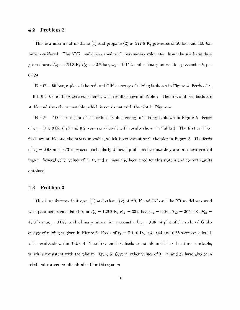
This is a mixture of methane (1) and propane (2) at 277.6 K; pressures of 50 bar and 100 bar

were considered. The SRK model was used with parameters calculated from the methane data

given above, Tc2 = 369.8 K, Pc2 = 42.5 bar, !2 = 0.152, and a binary interaction parameter k12 =

0.029.

For P = 50 bar, a plot of the reduced Gibbs energy of mixing is shown in Figure 4. Feeds of z1

= 0.1, 0.4, 0.6 and 0.9 were considered, with results shown in Table 2. The �rst and last feeds are

stable and the others unstable, which is consistent with the plot in Figure 4.

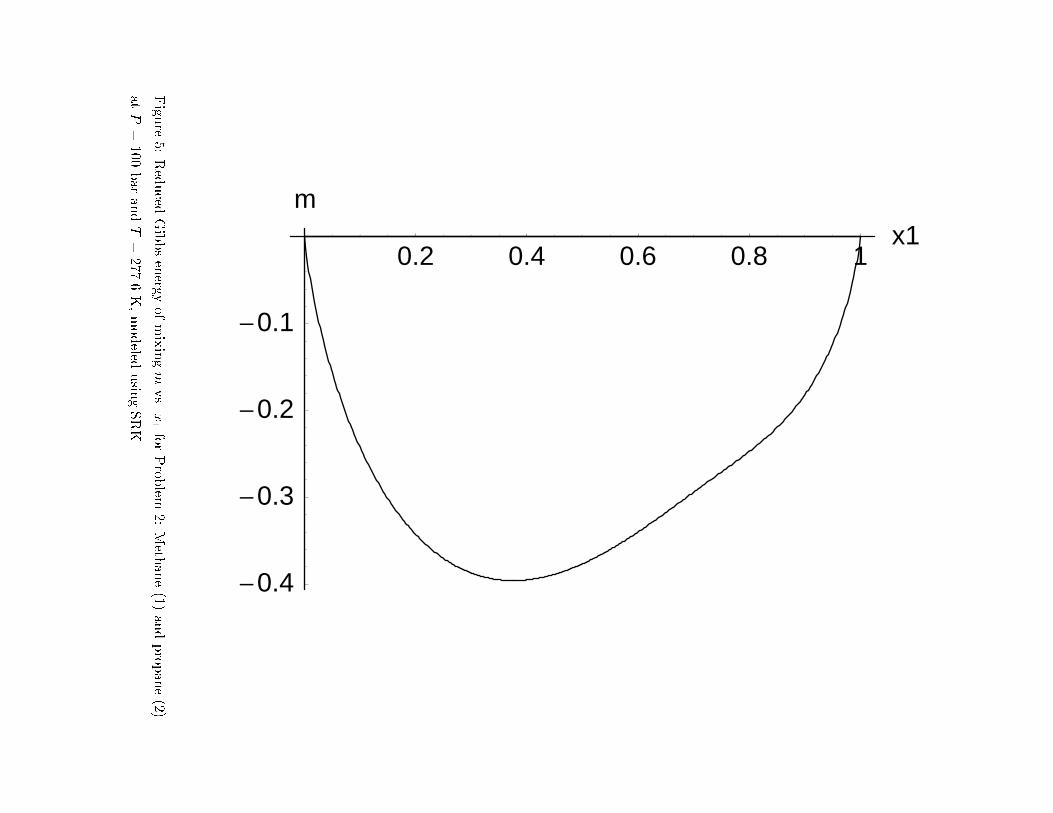
For P = 100 bar, a plot of the reduced Gibbs energy of mixing is shown in Figure 5. Feeds

of z1 = 0.4, 0.68, 0.73 and 0.9 were considered, with results shown in Table 3. The �rst and last

feeds are stable and the others unstable, which is consistent with the plot in Figure 5. The feeds

of z1 = 0.68 and 0.73 represent particularly di�cult problems because they are in a near critical

region. Several other values of T , P , and z1 have also been tried for this system and correct results

obtained.

4.3 Problem 3

This is a mixture of nitrogen (1) and ethane (2) at 270 K and 76 bar. The PR model was used

with parameters calculated from Tc1 = 126.2 K, Pc1 = 33.9 bar, !1 = 0.04 , Tc2 = 305.4 K, Pc2 =

48.8 bar, !2 = 0.098, and a binary interaction parameter k12 = 0.08. A plot of the reduced Gibbs

energy of mixing is given in Figure 6. Feeds of z1 = 0.1, 0.18, 0.3, 0.44 and 0.65 were considered,

with results shown in Table 4. The �rst and last feeds are stable and the other three unstable,

which is consistent with the plot in Figure 6. Several other values of T , P , and z1 have also been

tried and correct results obtained for this system.

10

4.4 Problem 4

This is a mixture of carbon dioxide (1) and methane (2) at 220 K and 60.8 bar. The PR

model was used with parameters calculated from Tc1 = 304.2 K, Pc1 = 73.8 bar, !1 = 0.225 , the

methane parameters given above, and a binary interaction parameter k12 = 0.095. A plot of the

reduced Gibbs energy of mixing is given in Figure 7. Feeds of z1 = 0.1, 0.2, 0.3, 0.43 and 0.6 were

considered, with results shown in Table 5. The �rst and last feeds are stable and the other three

unstable, which is consistent with the plot in Figure 7. Several other values of T , P , and z1 have

also been tried and correct results obtained for this system. While this problem and those above

involve binary mixtures, the method is applicable to problems with any number of components,

and tests involving ternary and larger systems are under way.

4.5 Discussion

In the problems above we used IN/GB to �nd all the stationary points. However, for making

a determination of phase stability or instability, �nding all the stationary points is not always

necessary. For example if an interval is encountered over which the interval evaluation of D has

a negative upper bound, this guarantees that there is a point at which D < 0, and so one can

immediately conclude that the mixture is unstable without determining all the stationary points.

It is also possible to make use of the underlying global minimization problem. Since the objective

function D has a known value of zero at the mixture feed composition, any interval over which the

interval value of D has a lower bound greater than zero cannot contain the global minimum and

can be discarded, even though it may contain a stationary point (at which D will be positive and

thus not of interest).

Finally it should be noted that the method described here can easily be combined with existing

11

local methods for determining phase stability. First, the (fast) local method is used. If it indicates

instability then this is the correct answer as it means a point at which D < 0 has been found. If

the local method indicates stability, however, this may not be the correct answer since the local

method may have missed the global minimum in D. Applying the new method described here can

then be used to con�rm that the mixture is stable if that is the case, or to correctly determine that

it is really unstable if that is the case.

5 Conclusions and Signi�cance

Results demonstrate that the interval Newton/generalized bisection algorithm can solve phase

stability problems for a generalized cubic equation of state model e�ciently and with complete

reliability. This work represents an entirely new method for solving these problems, a method that

can guarantee with mathematical certainty that the correct solutions are found, thus eliminating

computational problems that are frequently encountered with currently available techniques. The

method is initialization independent; it is also model independent, straightforward to use, and can

be applied in connection with other equations of state or with activity coe�cient models.

Acknowledgments { This work has been supported in part by the donors of The Petroleum

Research Fund, administered by the ACS, under Grant 30421-AC9, by the National Science Foun-

dation Grants CTS95-22835 and DMI96-96110, by the Environmental Protection Agency Grant

R824731-01-0, and by the Department of Energy Grant DE-FG07-96ER14691.

12

References

Baker, L. E., A. C. Pierce, and K. D. Luks, Gibbs energy analysis of phase equilibria. Soc. Petrol.

Engrs. J., 22, 731{742 (1982).

Balaji, G. V. and J. D. Seader, Application of interval-newton method to chemical engineering

problems. AIChE Symp. Ser, 91(304), 364{367 (1995).

Eubank, A. C., A. E. Elhassan, M. A. Barrufet, and W. B. Whiting, Area method for prediction

of uid-phase equilibria. Ind. Eng. Chem. Res., 31, 942{949 (1992).

Green, K. A., S. Zhou, and K. D. Luks, The fractal response of robust solution techniques to the

stationary point problem. Fluid Phase Equilibria, 84, 49{78 (1993).

Hansen, E. R., Global Optimization Using Interval Analysis. Marcel Dekkar, Inc., New York (1992).

Hansen, E. R. and R. I. Sengupta, Bounding solutions of systems of equations using interval analysis.

BIT, 21, 203{211 (1981).

Hua, J. Z., J. F. Brennecke, and M. A. Stadtherr, Reliable prediction of phase stability using an

interval-Newton method. Fluid Phase Equilibria, 116, 52{59 (1996a).

Hua, J. Z., S. R. Tessier, W. C. Rooney, J. F. Brennecke, and M. A. Stadtherr, Enhanced interval

techniques for reliable computation of phase equilibrium. Presented at AIChE Annual Meeting,

Chicago, November, 1996b.

Hytoft, G. and R. Gani, IVC-SEP Program Package. Technical Report SEP 8623, Institut for

Kemiteknik, Danmarks Tekniske Universitet, Lyngby, Denmark (1996).

13

Kearfott, R. B., Interval arithmetic techniques in the computational solution of nonlinear systems

of equations: Introduction, examples, and comparisons. Lectures in Applied Mathematics, 26,

337{357 (1990).

Kearfott, R. B., Rigorous Global Search: Continuous Problems. Kluwer Academic Publishers,

Dordrecht (1996).

Kearfott, R. B., M. Dawande, K.-S. Du, and C.-Y. Hu, Algorithm 737: INTLIB, a portable FOR-

TRAN 77 interval standard function library. ACM Trans. Math. Software, 20, 447{459 (1994).

Kearfott, R. B. and M. Novoa, Algorithm 681: INTBIS, a portable interval Newton/bisection

package. ACM Trans. Math. Software, 16, 152{157 (1990).

McDonald, C. M. and C. A. Floudas, Global optimization for the phase stability problem. AIChE

J., 41, 1798{1814 (1995a).

McDonald, C. M. and C. A. Floudas, Global optimization for the phase and chemical equilibrium

problem: Application to the NRTL equation. Comput. Chem. Eng., 19, 1111{1139 (1995b).

McDonald, C. M. and C. A. Floudas, Global optimization and analysis for the Gibbs free energy

function using the UNIFAC, Wilson, and ASOG equations. Ind. Eng. Chem. Res., 34, 1674{

1687 (1995c).

McDonald, C. M. and C. A. Floudas, GLOPEQ: A new computational tool for the phase and

chemical equilibrium problem. Comput. Chem. Eng., 21, 1{23 (1997).

McKinnon, K. I. M., C. G. Millar, and M. Mongeau, Global optimization for the chemical and

phase equilibrium problem using interval analysis. In Floudas, C. A. and P. M. Pardalos,

14

editors, State of the Art in Global Optimization: Computational Methods and Applications.

Kluwer Academic Publishers (1996).

Michelsen, M. L., The isothermal ash problem. Part I: Stability. Fluid Phase Equilibria, 9, 1{19

(1982).

Moore, R. E., Interval Analysis. Prentice-Hall, Englewood Cli�s (1966).

Nagarajan, N. R., A. S. Cullick, and A. Griewank, New strategy for phase equilibrium and critical

point calculations by thermodynamic energy analysis. Part I. Stability analysis and ash. Fluid

Phase Equilibria, 62, 191{210 (1991).

Neumaier, A., Interval Methods for Systems of Equations. Cambridge University Press, Cambridge,

England (1990).

Reid, R. C., J. M. Prausnitz, and B. E. Poling, The Properties of Gases and Liquids. McGraw-Hill

(1987).

Schnepper, C. A. and M. A. Stadtherr, On using parallel processing techniques in chemical process

design. Presented at AIChE Annual Meeting, Chicago, November, 1990.

Schnepper, C. A. and M. A. Stadtherr, Robust process simulation using interval methods. Comput.

Chem. Eng., 20, 187{199 (1996).

Stadtherr, M. A., C. A. Schnepper, and J. F. Brennecke, Robust phase stability analysis using

interval methods. AIChE Symp. Ser., 91(304), 356{359 (1995).

Sun, A. C. and W. D. Seider, Homotopy-continuation method for stability analysis in the global

minimization of the Gibbs free energy. Fluid Phase Equilibria, 103, 213{249 (1995).

15

Wasylkiewicz, S. K., L. N. Sridhar, M. F. Malone, and M. F. Doherty, Global stability analysis and

calculation of liquid-liquid equilibrium in multicomponent mixtures. Ind. Eng. Chem. Res.,

35, 1395{1408 (1996).

16

Figure Captions

Figure 1. Reduced Gibbs energy of mixing m vs. x1 for Problem 1: Hydrogen sul�de (1) and

methane (2) at P = 40.53 bar and T = 190 K, modeled using SRK.

Figure 2. Tangent plane distance D vs. x1 for Problem 1 with feed composition z1 = 0:0187. See

Figure 3 for enlargement of area near the origin.

Figure 3. Enlargement of part of Figure 2, showing area near the origin.

Figure 4. Reduced Gibbs energy of mixing m vs. x1 for Problem 2: Methane (1) and propane (2)

at P = 50 bar and T = 277.6 K, modeled using SRK.

Figure 5. Reduced Gibbs energy of mixing m vs. x1 for Problem 2: Methane (1) and propane (2)

at P = 100 bar and T = 277.6 K, modeled using SRK.

Figure 6. Reduced Gibbs energy of mixing m vs. x1 for Problem 3: Nitrogen (1) and ethane (2)

at P = 76 bar and T = 270 K, modeled using PR.

Figure 7. Reduced Gibbs energy of mixing m vs. x1 for Problem 4: Carbon dioxide (1) and

methane (2) at P = 60.8 bar and T = 220 K, modeled using PR.

17

Table 1: Results for Problem 1: Hydrogen sul�de (1) and methane (2) at P = 40.53 bar and T =

190 K, modeled using SRK.

Number of Root CPU Time (sec)

Feed (z1; z2) Roots (x1; x2; v) D Inclusion Tests Sun Ultra 1/170

(0.0115, 0.9885) (0.0115, 0.9885, 212.8) 0.0 5424 1.024

(0.0237, 0.9763, 97.82) 0.0137

(0.0326, 0.9674, 78.02) 0.0130

(0.0187, 0.9813) (0.8848, 0.1152, 36.58) 0.0109 8438 1.671

(0.0187, 0.9813, 207.3) 0.0

(0.0313, 0.9687, 115.4) 0.0079

(0.0767, 0.9233, 64.06) -0.004

(0.4905, 0.5095, 41.50) 0.0729

(0.07, 0.93) (0.8743, 0.1257, 36.65) 0.0512 8504 1.690

(0.5228, 0.4772, 40.89) 0.0965

(0.0178, 0.9822, 208.0) 0.0015

(0.0304, 0.9696, 113.7) 0.0100

(0.07 , 0.93 , 65.35) 0.0

(0.50, 0.50) (0.8819, 0.1181, 36.60) -0.057 8406 1.660

(0.0184, 0.9816, 207.5) -0.079

(0.0311, 0.9689, 114.9) -0.071

(0.0746, 0.9254, 64.44) -0.082

(0.50 , 0.50 , 41.32) 0.0

(0.888, 0.112) (0.888 , 0.112 , 36.55) 0.0 8396 1.671

(0.0190, 0.9810, 207.1) 0.0026

(0.0316, 0.9684, 116.0) 0.0103

(0.0792, 0.9208, 63.60) -0.002

(0.4795, 0.5205, 41.72) 0.0683

(0.89, 0.11) (0.89 , 0.11 , 36.54) 0.0 8410 1.673

(0.0192, 0.9808, 206.9) 0.0113

(0.0319, 0.9681, 116.4) 0.0189

(0.0809, 0.9191, 63.31) 0.0058

(0.4725, 0.5275, 41.87) 0.0724

18

Table 2: Results for Problem 2: Methane (1) and propane (2) at P = 50 bar and T = 277.6 K,

modeled using SRK.

Number of Root CPU Time (sec)

Feed (z1; z2) Roots (x1; x2; v) D Inclusion Tests Sun Ultra 1/170

(0.10, 0.90) (0.10 , 0.90 , 86.71) 0.0 1969 0.413

(0.40, 0.60) (0.8654, 0.1346, 378.4) -0.153 4345 0.905

(0.5515, 0.4485, 115.3) 0.0106

(0.40 , 0.60 , 89.46) 0.0

(0.60, 0.40) (0.7058, 0.2942, 313.0) -0.007 3706 0.782

(0.60 , 0.40 , 216.5) 0.0

(0.1928, 0.8072, 86.07) -0.223

(0.90, 0.10) (0.90 , 0.10 , 388.5) 0.0 3290 0.640

19

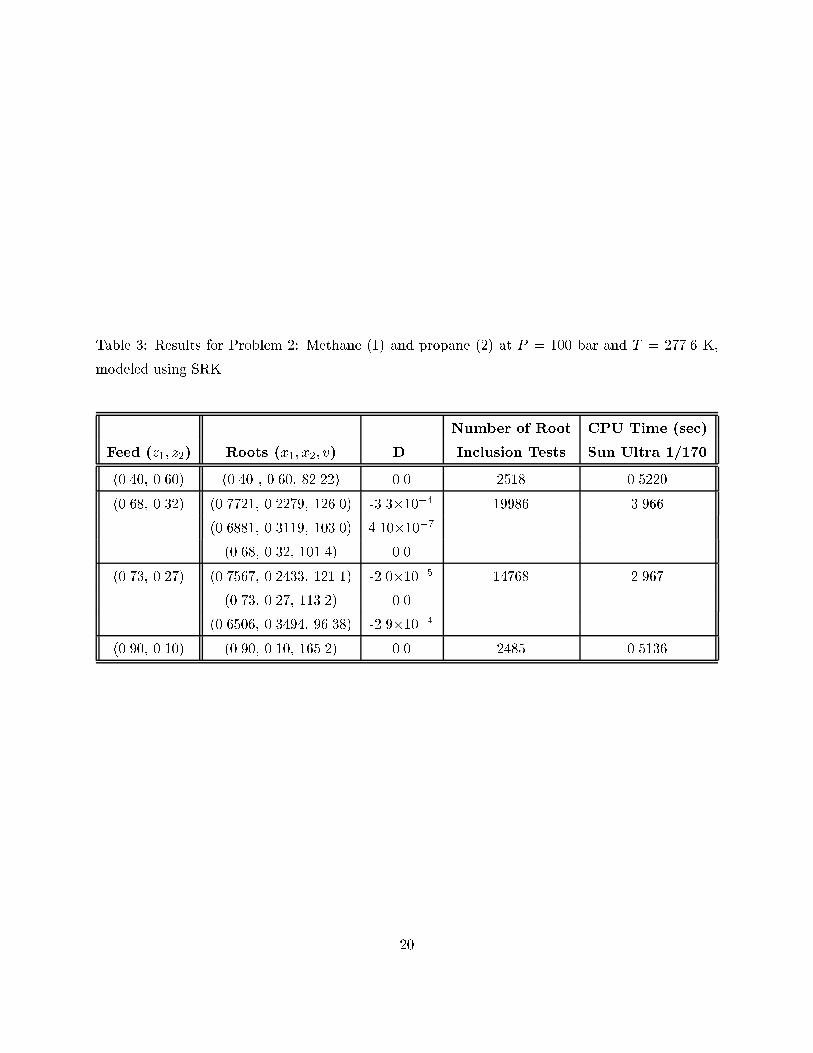
Table 3: Results for Problem 2: Methane (1) and propane (2) at P = 100 bar and T = 277.6 K,

modeled using SRK.

Number of Root CPU Time (sec)

Feed (z1; z2) Roots (x1; x2; v) D Inclusion Tests Sun Ultra 1/170

(0.40, 0.60) (0.40 , 0.60, 82.22) 0.0 2518 0.5220

(0.68, 0.32) (0.7721, 0.2279, 126.0) -3.3�10�4 19986 3.966

(0.6881, 0.3119, 103.0) 4.10�10�7(0.68, 0.32, 101.4) 0.0

(0.73, 0.27) (0.7567, 0.2433, 121.1) -2.0�10�5 14768 2.967

(0.73, 0.27, 113.2) 0.0

(0.6506, 0.3494, 96.38) -2.9�10�4(0.90, 0.10) (0.90, 0.10, 165.2) 0.0 2485 0.5136

20

Table 4: Results for Problem 3: Nitrogen (1) and ethane (2) at P = 76 bar and T = 270 K, modeled

using PR.

Number of Root CPU Time (sec)

Feed (z1; z2) Roots (x1; x2; v) D Inclusion Tests Sun Ultra 1/170

(0.10, 0.90) (0.10 , 0.90 , 71.11) 0.0 1881 0.4004

(0.18, 0.82) (0.4943, 0.5057, 198.3) -0.010 4560 0.9791

(0.2961, 0.7039, 110.4) 0.0058

(0.18 , 0.82 , 78.61) 0.0

(0.30, 0.70) (0.4893, 0.5107, 198.3) -0.0138 4586 0.9804

(0.30, 0.70, 112.3) 0.0

(0.1767, 0.8233, 78.18) -0.007

(0.44, 0.56) (0.44, 0.56, 181.2) 0.0 4649 0.9914

(0.3353, 0.6647, 131.5) 0.0026

(0.1547, 0.8453, 75.64) -0.016

(0.60, 0.40) (0.60, 0.40, 227.8) 0.0 3312 0.6506

21

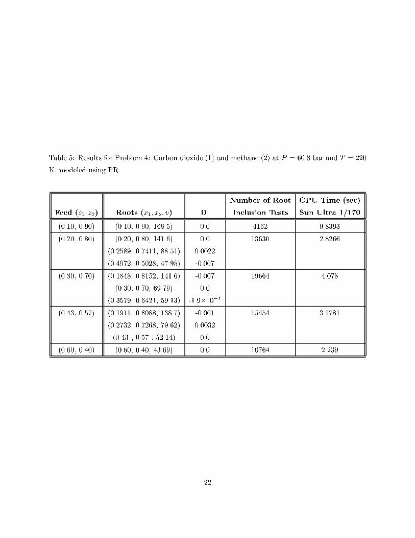
Table 5: Results for Problem 4: Carbon dioxide (1) and methane (2) at P = 60.8 bar and T = 220

K, modeled using PR.

Number of Root CPU Time (sec)

Feed (z1; z2) Roots (x1; x2; v) D Inclusion Tests Sun Ultra 1/170

(0.10, 0.90) (0.10, 0.90, 168.5) 0.0 4162 0.8393

(0.20, 0.80) (0.20, 0.80, 141.6) 0.0 13630 2.8266

(0.2589, 0.7411, 88.51) 0.0022

(0.4972, 0.5028, 47.98) -0.007

(0.30, 0.70) (0.1848, 0.8152, 141.6) -0.007 19664 4.078

(0.30, 0.70, 69.79) 0.0

(0.3579, 0.6421, 59.13) -1.9�10�4(0.43, 0.57) (0.1911, 0.8088, 138.7) -0.001 15454 3.1781

(0.2732, 0.7268, 79.62) 0.0032

(0.43 , 0.57 , 52.14) 0.0

(0.60, 0.40) (0.60, 0.40, 43.69) 0.0 10764 2.239

22

0.2 0.4 0.6 0.8 1x1

-0.08

-0.06

-0.04

-0.02

m

Figu

re1:

Reduced

Gibbsenergy

ofmixingm

vs.

x1for

Prob

lem1:

Hydrogen

sul�de(1)

and

meth

ane(2)

atP

=40.53

bar

andT=

190K,modeled

usin

gSRK.

0.2 0.4 0.6 0.8 1x1

0.02

0.04

0.06

0.08

0.1D

Figu

re2:

Tangen

tplan

edistan

ceD

vs.

x1for

Prob

lem1with

feedcom

position

z1=0:0187.

See

Figu

re3for

enlargem

entof

areanear

theorigin

.

0.05 0.1 0.15 0.2x1

0.005

0.01

0.015

0.02

D

Figu

re3:

Enlargem

entof

part

ofFigu

re2,

show

ingarea

near

theorigin

.

0.2 0.4 0.6 0.8 1x1

-0.25

-0.2

-0.15

-0.1

-0.05

m

Figu

re4:

Reduced

Gibbsenergy

ofmixingm

vs.x1for

Prob

lem2:

Meth

ane(1)

andprop

ane(2)

atP

=50

bar

andT=

277.6K,modeled

usin

gSRK.

0.2 0.4 0.6 0.8 1x1

-0.4

-0.3

-0.2

-0.1

m

Figu

re5:

Reduced

Gibbsenergy

ofmixingm

vs.x1for

Prob

lem2:

Meth

ane(1)

andprop

ane(2)

atP

=100

bar

andT=

277.6K,modeled

usin

gSRK.

0.2 0.4 0.6 0.8 1x1

-0.35

-0.3

-0.25

-0.2

-0.15

-0.1

-0.05

m

Figu

re6:

Reduced

Gibbsenergy

ofmixingm

vs.

x1for

Prob

lem3:

Nitrogen

(1)andeth

ane(2)

atP

=76

bar

andT=

270K,modeled

usin

gPR.

0.2 0.4 0.6 0.8 1x1

-0.25

-0.2

-0.15

-0.1

-0.05

m

Figu

re7:

Reduced

Gibbsenergy

ofmixingm

vs.x1for

Prob

lem4:

Carb

ondiox

ide(1)

andmeth

ane

(2)at

P=

60.8bar

andT=

220K,modeled

usin

gPR.