Performance Optimization of Scientific...
269
Performance Optimization of Scientific Applications Philip J. Mucci [email protected] Innovative Computing Laboratory, UTK Knoxville, TN PDC, KTH, Stockholm, Sweden
Transcript of Performance Optimization of Scientific...
Performance Optimization of Scientific Applications
Philip J. [email protected]
Innovative Computing Laboratory, UTK Knoxville, TN
PDC, KTH, Stockholm, Sweden

Outline
● Introduction● Important Facts about RISC Architecture● Performance Metrics and Issues● Compiler Technology● Serial Code Optimization● MPI/OpenMP Optimization● Numerical Libraries● Performance Analysis Tools

Introduction

Performance
● What is performance? ● Latency● Bandwidth● Efficiency● Scalability● Execution time
● At what cost?

Performance Examples
● Operation Weather Forecasting Model● Scalability
● Database search engine● Latency
● Image processing system● Throughput

What is Optimization?
● Finding hot spots & bottlenecks (profiling)● Code in the program that uses a
disproportional amount of time● Code in the program that uses system
resources inefficiently● Reducing wall clock time● Reducing resource requirements

Types of Optimization
● Hand-tuning● Preprocessor● Compiler● Parallelization

Steps of Optimization
● Integrate libraries● Optimize compiler switches ● Profile● Optimize blocks of code that dominate
execution time● Always examine correctness at every
stage!

Performance Strategies
● Always use optimal or near optimal algorithms.● Be careful of resource requirements and
problem sizes.● Maintain realistic and consistent input
data sets/sizes during optimization.● Know when to stop.

The 80/20 Rule
● Program spends 80 % time in 20 % of its code
● Programmer spends 20 % effort to get 80 % of the total speedup possible in the code.
“The Law of Diminishing Returns”

How high is up?
● Profiling reveals percentages of time spent in CPU and I/O bound functions.
● Correlation with representative low-level, kernel and application benchmarks.
● Literature search.● Peak speed of CPU means little in
relation to most codes.● Example: ISIS solver package

Don’t Sweat the Small Stuff● Make the Common Case Fast (Hennessey)
● A 20% decrease of procedure3()results in 10% increase in performance.
● A 20% decrease of main()results in 2.6% increase in performance
PROCEDURE TIMEmain() 13%procedure1() 17%procedure2() 20%
procedure3() 50%
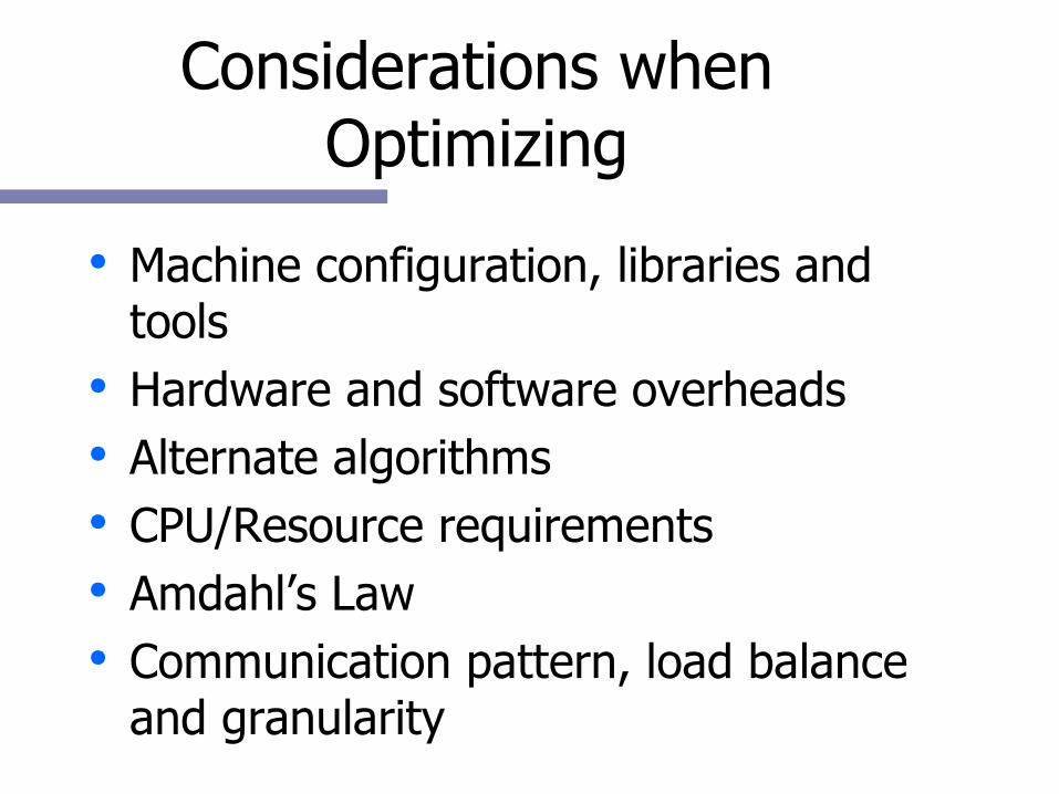
Considerations when Optimizing
● Machine configuration, libraries and tools
● Hardware and software overheads● Alternate algorithms ● CPU/Resource requirements● Amdahl’s Law● Communication pattern, load balance
and granularity

Important Facts about RISC Architecture

The Pipeline
● Instructions have latencies and bandwidths.
● Important to keep the pipeline full.● Avoid step by step dependencies in your
code.● A -> B● B -> C● C -> D

The RISC Philosophy
● Reduced Instruction Set Architecture● We can:
● Design, place and route more elegantly.● Drive a higher clock rate● Have a deeper pipeline.● Expose opportunities for instruction
parallelism to the compiler.● Guess what? Your Pentium is a RISC.
● CISC translated to RISC “micro-ops”.

The RISC Philosophy
● Reduced Instruction Set Architecture● If we:
● Keep the number of instructions small.● Keep the functionality of the instructions
orthogonal.● Keep the instructions isolated to one piece
of hardware on chip.
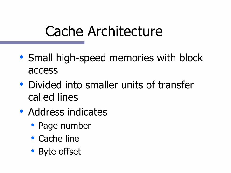
Cache Architecture
● Small high-speed memories with block access
● Divided into smaller units of transfer called lines
● Address indicates● Page number● Cache line● Byte offset
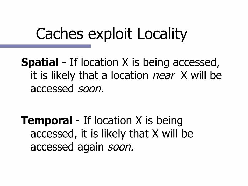
Caches exploit Locality
Spatial - If location X is being accessed, it is likely that a location near X will be accessed soon.
Temporal - If location X is being accessed, it is likely that X will be accessed again soon.

Cache Benchmarkhttp://www.cs.utk.edu/~mucci/cachebench
do i = 1,max_length
start_time
do j = 1,max_iterations
do k = 1,i
A(k) = i
enddo
enddo
stop_time_and_print
enddo

Cache Performance

Cache Mapping
● Two major types of mapping● Direct Mapped
Each memory address resides in only one cache line. (constant hit time)
● N-way Set AssociativeEach memory address resides in one of N cache lines. (variable hit time)
● Origin is 2-way set associative, 2-way interleaved

2 way Set Associative Cache
distinct lines = size / line size * associativity
Every datum can live in any set but in only 1 line (computed from its address)
Which class? Least Recently Used
Line0Set0
Line1Set0
Line2Set0
Line3Set0
Line0Set1
Line1Set1
Line2Set1
Line3Set1

The Register Set
● Register access is almost free.● Can be considered a level 0 cache.● # of registers is also limited.● Many processors contain virtual registers
that get renamed to physical registers at execution time.

What is a TLB?
● Fully associative cache of virtual to physical address mappings. Used if data not in cache.
● Number is limited on many systems, usually much less than physical memory.

Contention for Shared Resources
● Most SMP's these days have fewer memory buses than processors.
● Most SMP's share some level of cache.● Interconnect is also shared among
processes.

Performance Metrics and Issues
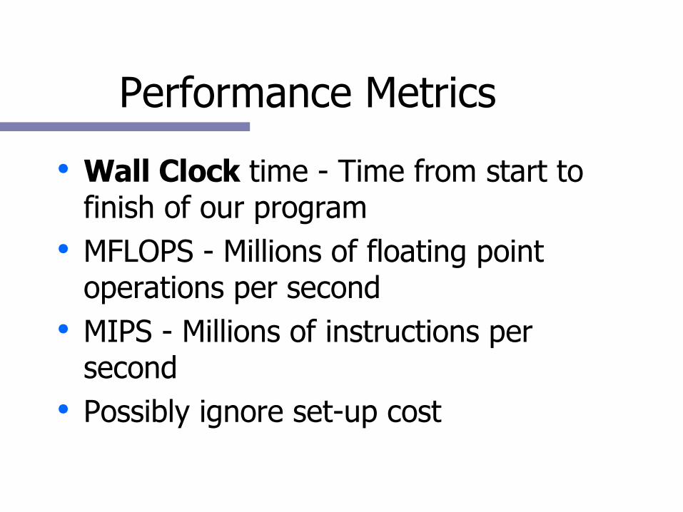
Performance Metrics
● Wall Clock time - Time from start to finish of our program
● MFLOPS - Millions of floating point operations per second
● MIPS - Millions of instructions per second
● Possibly ignore set-up cost

What about MFLOPS?
● Poor measures of comparison because● They are dependent on the definition,
instruction set and the compiler● Ok measures of numerical kernel
performance for a single CPU
EXECUTION TIME

What do we use for evaluation
● For purposes of optimization, we are interested in:● Execution time of our code over a range of
data sets● MFLOPS of our kernel code vs. peak in
order to determine EFFICIENCY● Hardware resources dominating our
execution time

Performance Metrics
For the purposes of comparing your codes performance among different architectures base your comparison on time.
...Unless you are completely aware of all the issues in performance analysis including architecture, instruction sets, compiler technology etc...

Fallacies● MIPS is an accurate measure for comparing
performance among computers. ● MFLOPS is a consistent and useful measure of
performance among computers.● Synthetic benchmarks predict performance for real
programs.● Peak performance tracks observed performance.
(Hennessey and Patterson)

Basis for Performance Analysis
● Our evaluation will be based upon:● Performance of a single machine on a ● Single (optimal) algorithm using● Execution time
● Optimizations are portable

Asymptotic Analysis
● Algorithm X requires O(N log N) time on O(N processors)
● This ignores constants and lower order terms!
10N > N log N for N < 102410N*N < 1000N log N for N < 996

Amdahl’s Law
● The performance improvement is limited by the fraction of time the faster mode can be used.
Speedup = Perf. enhanced / Perf. standardSpeedup = Time sequential / Time parallel
Time parallel = Tser + Tpar

Amdahl’s Law
● Be careful when using speedup as a metric. Ideally, use it only when the code is modified. Be sure to completely analyze and document your environment.
● Problem: This ignores the overhead of parallel reformulation.

Amdahl’s Law
● Problem? This ignores scaling of the problem size with number of nodes.
● Ok, what about Scaled Speedup?● Scale the problem size with the # procs.● Results will vary given the nature of the
algorithm.● Requires O() analysis of communication
and run-time operations.

Efficiency
● A measure of code quality?
E = Time sequential / ( P * Time parallel)S = P * E
● Sequential time is not a good reference point.
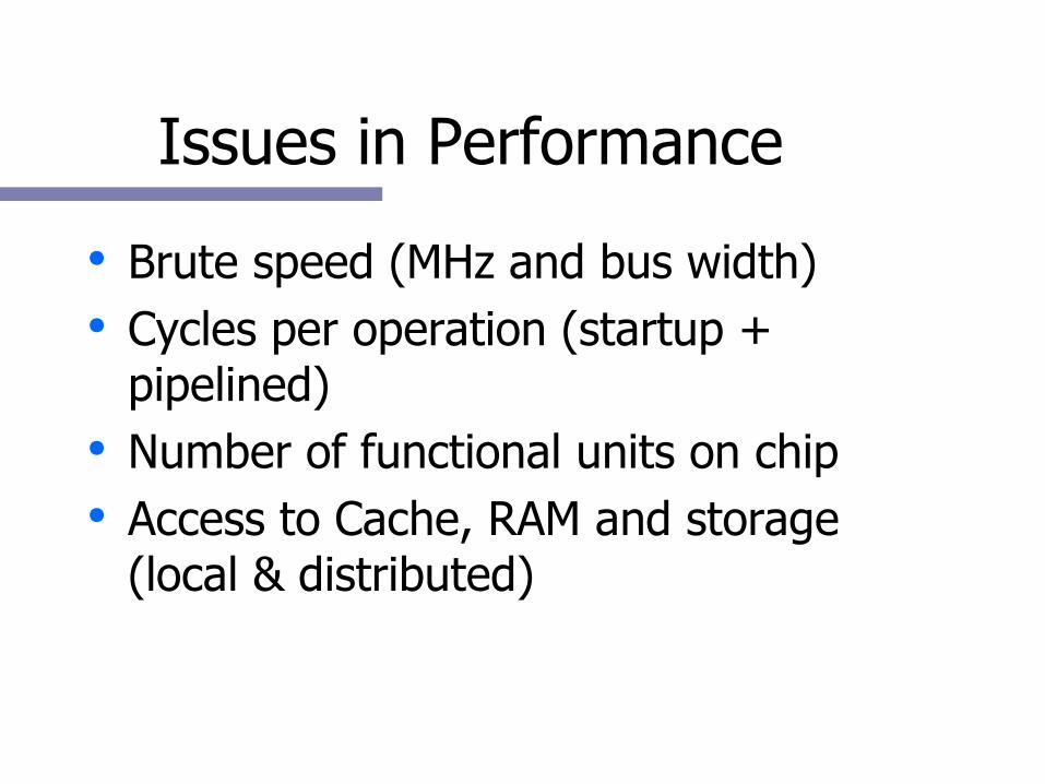
Issues in Performance
● Brute speed (MHz and bus width)● Cycles per operation (startup +
pipelined)● Number of functional units on chip● Access to Cache, RAM and storage
(local & distributed)
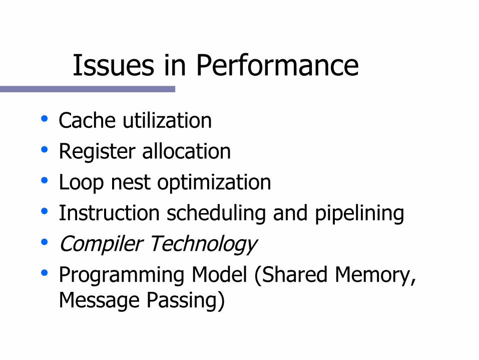
Issues in Performance
● Cache utilization● Register allocation● Loop nest optimization● Instruction scheduling and pipelining● Compiler Technology● Programming Model (Shared Memory,
Message Passing)

Problem Size and Precision
● Necessity● Density and Locality ● Memory, Communication and Disk I/O● Numerical representation
● INTEGER, REAL, REAL*8, REAL*16
Parallel Performance Issues
● Single node performance● Compiler Parallelization● I/O and Communication● Mapping Problem - Load Balancing● Message Passing or Data Parallel
Optimizations

What is Optimization?
● Finding hot spots & bottlenecks (profiling)● Code in the program that uses a
disproportional amount of time● Code in the program that uses system
resources inefficiently● Reducing wall clock time● Reducing resource requirements

Types of Optimization
● Hand-tuning● Preprocessor● Compiler● Parallelization
Performance Strategies
● Use profiling tools before you optimize.● Always use optimal or near optimal
algorithms.● Be careful of requirements and problem
sizes.● The largest bottleneck first.● Maintain realistic and consistent input
data sets/sizes during optimization.● Know when to stop.

Considerations when Optimizing
Developer should be familiar with:● Machine configuration, libraries and
tools● Hardware and Software overheads● Algorithm and alternatives ● CPU/Resource requirements● Amdahl’s Law● Communication patterns and load
balance

Correctness at Every Step
● Floating point arithmetic is not associative. Which order is correct?
● Think about the following example:
sum = 0.0
do i = 1, n
sum = sum + a(i)
enddo
sum1 = 0.0
sum2 = 0.0
do i = 1, n-1, 2
sum1 = sum1 + a(i)
sum2 = sum2 + a(i+1)
enddo
sum = sum1 + sum2

Compiler Technology
Understanding Compilers
● Compilers emphasize correctness rather than performance
● On well recognized constructs, compilers will usually do better than the developer
● The idea? To express an algorithm clearly to the compiler allows the most optimization.

Compiler Technology
● Ideally, compiler should do most of the work.
● Rarely happens in practice for real applications.
● Getting better every day.

Compiler flags
● Many optimizations can be controlled separately from -O<big>
● If possible, it's better to selectively disable optimizations rather than reduce the level of global optimization.

Exceptions
● Numerical computations resulting in undefined results or requiring assistance.
● Exception is generated by the processor.
● Handled in software by the Operating System.
● DENORM's are the worst.
Pointer Aliasing
● The compiler needs to assume that any 2 pointers can point to the same region of memory.
● This removes many optimization opportunities.
● Programmer knows much more about pointer usage than compiler, try to express it with directives.

Advanced Aliasing
● Typed: Only pointers of the same type can point to the same region of memory.
● Restricted: All pointers are assumed to point to non-overlapping regions of memory.
● Disjointed: All pointer expressions are assumed to result in pointers to non-overlapping regions of memory.
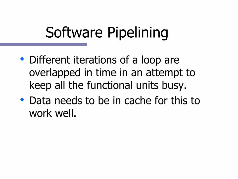
Software Pipelining
● Different iterations of a loop are overlapped in time in an attempt to keep all the functional units busy.
● Data needs to be in cache for this to work well.

Interprocedural Analysis
● When analysis is confined to a single procedure, the optimizer is forced to make worst case assumptions about the possible effects.
● IPA analyzes more of the code and feeds that to the other phases.
● Usually, the code is generated at link time.

IPA features
● Inlining across source files● Common block padding● Constant propagation● Dead function/variable elimination● Library reference optimizations

Inlining
● Replaces a subroutine call with the function itself.
● Useful in loops that have a large iteration count and functions that don’t do a lot of work.
● Allows other optimizations.● Most compilers will do inlining but the
decision process is conservative.

Serial Code Optimization

Parallel Performance
“The single most important impediment to good parallel
performance is still poor single-node performance.”
- William GroppArgonne National Lab

Guidelines for Performance
● I/O is slow● System calls are slow● Use your in-cache data completely● When looping, remember the pipeline!
● Branches● Function calls● Speculation/Out-of-order execution● Dependencies
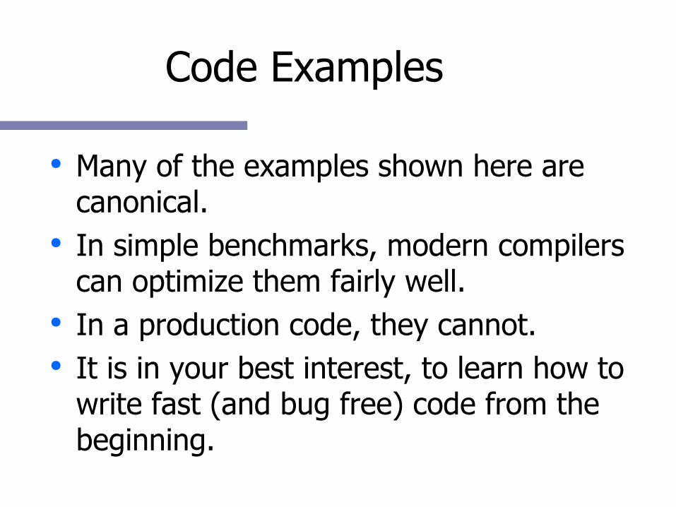
Code Examples
● Many of the examples shown here are canonical.
● In simple benchmarks, modern compilers can optimize them fairly well.
● In a production code, they cannot.● It is in your best interest, to learn how to
write fast (and bug free) code from the beginning.

Array Optimization
● Array Initialization● Array Padding● Stride Minimization● Loop Fusion● Floating IF’s● Loop Defactorization● Loop Peeling● Loop Interchange
● Loop Collapse● Loop Unrolling● Loop Unrolling and
Sum Reduction● Outer Loop Unrolling
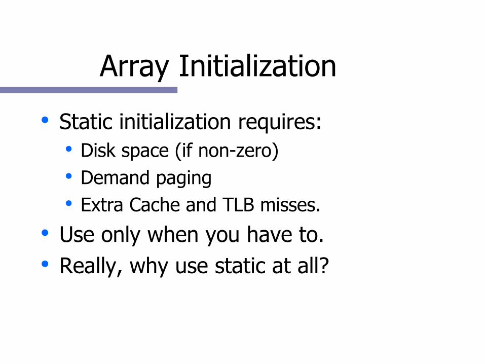
Array Initialization
● Static initialization requires:● Disk space (if non-zero)● Demand paging● Extra Cache and TLB misses.
● Use only when you have to.● Really, why use static at all?
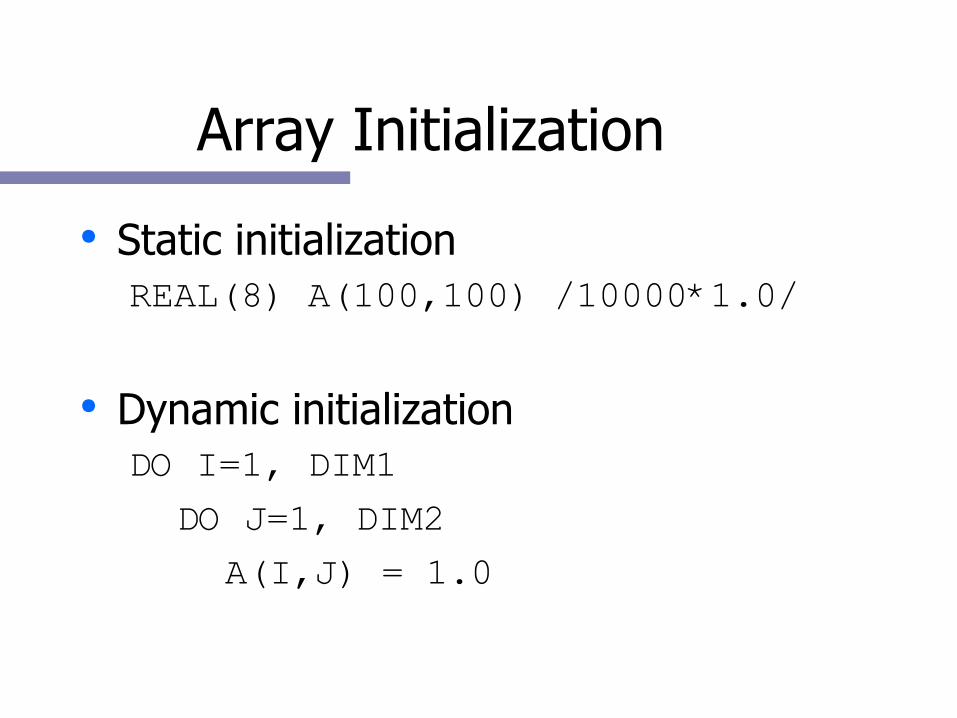
Array Initialization
● Static initializationREAL(8) A(100,100) /10000*1.0/
● Dynamic initializationDO I=1, DIM1
DO J=1, DIM2
A(I,J) = 1.0
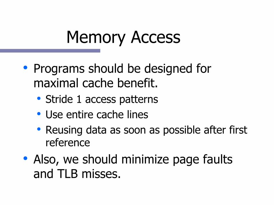
Memory Access
● Programs should be designed for maximal cache benefit.● Stride 1 access patterns● Use entire cache lines● Reusing data as soon as possible after first
reference● Also, we should minimize page faults
and TLB misses.

Array Allocation
● Array’s are allocated differently in C and FORTRAN.
1 2 3 4
5 6 7 8
9 10 11 12
C: 1 2 3 4 5 6 7 8 9 10 11 12
Fortran: 1 5 9 2 6 10 3 7 11 4 8 12

Array Referencing
● In C, outer-most index should change fastest.
[x,Y]● In Fortran, inner-most index should
change fastest.(X,y)
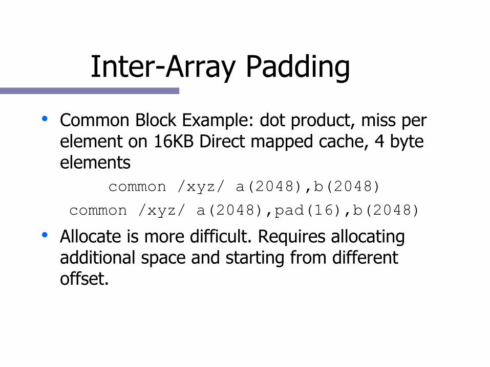
Inter-Array Padding● Common Block Example: dot product, miss per
element on 16KB Direct mapped cache, 4 byte elements
common /xyz/ a(2048),b(2048)
common /xyz/ a(2048),pad(16),b(2048)
● Allocate is more difficult. Requires allocating additional space and starting from different offset.

Inter-Array Padding
● Data is often allocated in physically contiguous memory and on a page boundary.
● Look for data structures whose size is a powers of two
● Know the associativity of your cache.● Watch for performance anomalies.

Inter-Array Padding

Inter-Array Paddinga = a + b * c
Tuned Untuned Tuned-O3
Untuned-O3
Origin2000 1064.1 1094.7 800.9 900.3

Intra-Array Padding
● Often required by matrix operations when striding across each dimension.
● C: Trailing dimension of a power of two is often a bad choice.
● Fortran: Leading dimension of a power of two is often a bad choice.
● This depends on the degree of associativity of the cache.

Intra-Array PaddingDGEMM
Tuned Untuned
Xeon 2.8 3.3

Stride Minimization
● We must think about spatial locality.● Effective usage of the cache provides us
with the best possibility for a performance gain.
● Recently accessed data are likely to be faster to access.
● Tune your algorithm to minimize stride, innermost index changes fastest.

Stride Minimization
● Stride 1do y = 1, 1000
do x = 1, 1000
c(x,y) = c(x,y) + a(x,y)*b(x,y)
● Stride 1000do y = 1, 1000
do x = 1, 1000
c(y,x) = c(y,x) + a(y,x)*b(y,x)

Stride Minimization
Untuned-O3
Tuned-O3
Origin2000
67.24 23.27
IBM SP2 201.07 17.54
Cray T3E 37.61 37.66

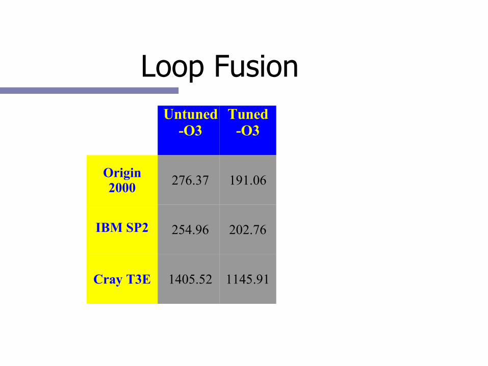
Loop Fusion
● Loop overhead reduced● Better instruction overlap● Lower cache misses● Be aware of associativity issues with
array’s mapping to the same cache line.

Loop Fusion
● Untuned
do i = 1, 50000
x = x * a(i) + b(i)
enddo
do i = 1, 100000
y = y + a(i) / b(i)
enddo
● Tuned
do i = 1, 50000
x = x * a(i) + b(i)
y = y + a(i) / b(i)
enddo
do i = 50001, 100000
y = y + a(i) / b(i)
enddo
Loop FusionUntuned
-O3Tuned
-O3
Origin2000
276.37 191.06
IBM SP2 254.96 202.76
Cray T3E 1405.52 1145.91

Loop Interchange
● Swapping the nested order of loops● Minimize stride● Reduce loop overhead where inner loop
counts are small● Allows better compiler scheduling

Loop Interchange
● Untuned
real*8 a(2,40,2000)
do i=1, 2000
do j=1, 40
do k=1, 2
a(k,j,i) = a(k,j,i)*1.01
enddo
enddo
enddo
● Tuned
real*8 a(2000,40,2)
do i=1, 2
do j=1, 40
do k=1, 2000
a(k,j,i) = a(k,j,i)*1.01
enddo
enddo
enddo
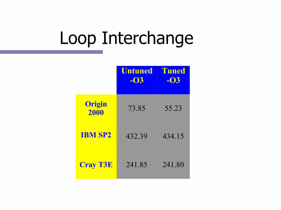
Loop Interchange
Untuned-O3
Tuned-O3
Origin2000
73.85 55.23
IBM SP2 432.39 434.15
Cray T3E 241.85 241.80
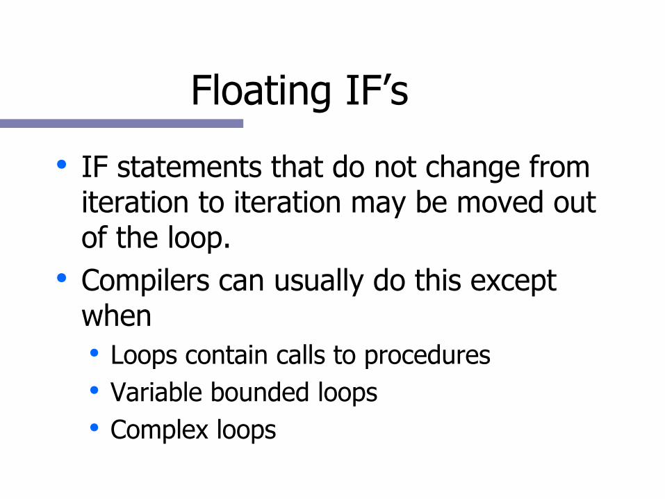
Floating IF’s
● IF statements that do not change from iteration to iteration may be moved out of the loop.
● Compilers can usually do this except when● Loops contain calls to procedures● Variable bounded loops● Complex loops

Floating IF’s
● Untuned
do i = 1, lda
do j = 1, lda
if (a(i) .GT. 100) then
b(i) = a(i) - 3.7
endif
x = x + a(j) + b(i)
enddo
enddo
● Tuned
do i = 1, lda
if (a(i) .GT. 100) then
b(i) = a(i) - 3.7
endif
do j = 1, lda
x = x + a(j) + b(i)
enddo
enddo
Floating IF’s
Untuned –O3
Tuned –O3
Origin2000
203.18 94.11
IBMSP2
80.56 80.77
CrayT3E
160.86 161.21

Loop Defactorization
● Loops involving multiplication by a constant in an array.
● Allows better instruction scheduling.● Facilitates use of multiply-adds.

Gather-Scatter Optimization
● Untuned
do i = 1, n
if (t(I).gt.0.0) then
a(I)=2.0*b(I-1)
end if
enddo
● Tuned
inc = 0
do i = 1, n
tmp(inc) = i
if (t(I).gt.0.0) then
inc = inc + 1
end if
enddo
do I = 1, inc
a(tmp(I))=2.0*b((tmp(I)-1)
enddo

Gather-Scatter Optimization
● For loops with branches inside loops● Increases pipelining● Often, body of the loop is executed on
every iteration, thus no savings● Solution is to split the loop with a
temporary array containing indices of elements to be computed with

IF Statements in Loops
● Solution is to unroll the loop● Move conditional elements into scalars● Test scalars at the end of the loop bodydo I = 1, n, 2
a = t(I)
b = t(I+1)
if (a .eq. 0.0)
end if
if (b .eq. 0.0)
end if
end do

Loop Defactorization
● Note that floating point operations are not always associative.
(A + B) + C != A + (B + C)
● Be aware of your precision● Always verify your results with
unoptimized code first!

Loop Defactorization
● Untuned
do i = 1, lda
A(i) = 0.0
do j = 1, lda
A(i)=A(i)+B(j)*D(j)*C(i)
enddo
enddo
● Tuned
do i = 1, lda
A(i) = 0.0
do j = 1, lda
A(i) = A(i) + B(j) * D(j)
enddo
A(i) = A(i) * C(i)
enddo
Loop DefactorizationTuned
-O3Untuned
-O3
Origin2000
371.95 559.17
IBM SP2 449.03 591.26
Cray T3E 3201.35 3401.61

Loop Peeling
● For loops which access previous elements in arrays.
● Compiler often cannot determine that an item doesn’t need to be loaded every iteration.

Loop Peeling
● Untuned
jwrap = lda
do i = 1, lda
b(i) = (a(i)+a(jwrap))*0.5
jwrap = i
enddo
● Tuned
b(1) = (a(1)+a(lda))*0.5
do i = 2, lda
b(i) = (a(i)+a(i-1))*0.5
enddo

Loop PeelingTuned
-O3Untuned
-O3
Origin2000
61.06 63.33
IBM SP2 25.68 40.50
Cray T3E 72.93 90.05

Loop Collapse
● For multi-nested loops in which the entire array is accessed.
● This can reduce loop overhead and improve compiler vectorization.

Loop Collapse
● Untuned do i = 1, lda do j = 1, ldb
do k = 1, ldc
A(k,j,i) = A(k,j,i) + B(k,j,i) * C(k,j,i)
enddo
enddo
enddo

Loop Collapse
● Tuned do i = 1, lda*ldb*ldc
A(i,1,1) = A(i,1,1) + B(i,1,1) * C(i,1,1)
enddo
● More Tuned (declarations are 1D) do i = 1, lda*ldb*ldc
A(i) = A(i) + B(i) * C(i)
enddo

Loop CollapseTuned Tuned
–O3Tuned
2nd Tuned 2nd
–O3
Origin2000
400.25 143.01 410.58 77.86
IBMSP2
144.75 31.57 144.18 31.54
CrayT3E
394.19 231.44 394.92 229.86
Loop Unrolling
● Data dependence delays can be reduced or eliminated.
● Reduce loop overhead.● Usually performed well by the compiler
or preprocessor.

Loop Unrolling
● Untuned
do i = 1, lda
do j = 1, lda
do k = 1, 4
a(j,i) = a(j,i) + b(i,k) * c(j,k)
enddo
enddo
enddo

Loop Unrolling
● Tuned (4)
do i = 1, lda
do j = 1, lda
a(j,i) = a(j,i) + b(i,1) * c(j,1)
a(j,i) = a(j,i) + b(i,2) * c(j,2)
a(j,i) = a(j,i) + b(i,3) * c(j,3)
a(j,i) = a(j,i) + b(i,4) * c(j,4)
enddo
enddo

Loop Unrolling
Tuned-O3
Untuned-O3
Origin2000
61.06 63.33
IBM SP2 11.26 12.65
Cray T3E 36.30 24.41
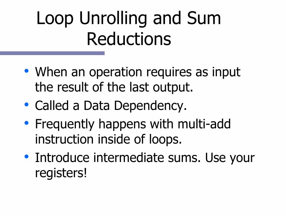
Loop Unrolling and Sum Reductions
● When an operation requires as input the result of the last output.
● Called a Data Dependency.● Frequently happens with multi-add
instruction inside of loops.● Introduce intermediate sums. Use your
registers!

Loop Unrolling and Sum Reductions
● Untuned
do i = 1, lda
do j = 1, lda
a = a + (b(j) * c(i))
enddo
enddo

Loop Unrolling and Sum Reductions
● Tuned (4)
do i = 1, lda
do j = 1, lda, 4
a1 = a1 + b(j) * c(i)
a2 = a2 + b(j+1) * c(i)
a3 = a3 + b(j+2) * c(i)
a4 = a4 + b(j+3) * c(i)
enddo
enddo
aa = a1 + a2 +a3 + a4

Loop Unrolling and Sum Reductions
Untuned–O3
2Tuned
2Tuned–O3
4Tuned
-O3
8Tuned
-O3
16Tuned
-O3
Origin2000
454 4945 352 350 350 330
IBMSP2
281 6490 563 281 281 263
CrayT3E 865 10064 564 340 231 860

Outer Loop Unrolling
● For nested loops, unrolling outer loop may reduce loads and stores in the inner loop.
● Compiler may perform this optimization.

Outer Loop Unrolling
● Untuned● Each flop requires two loads and one store.
do i = 1, lda
do j = 1, ldb
A(i,j) = B(i,j) * C(j)
enddo
enddo
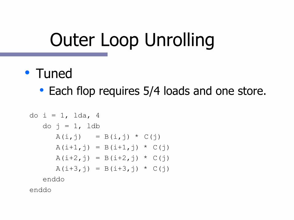
Outer Loop Unrolling
● Tuned● Each flop requires 5/4 loads and one store.
do i = 1, lda, 4
do j = 1, ldb
A(i,j) = B(i,j) * C(j)
A(i+1,j) = B(i+1,j) * C(j)
A(i+2,j) = B(i+2,j) * C(j)
A(i+3,j) = B(i+3,j) * C(j)
enddo
enddo

Outer Loop UnrollingTuned
-O3Untuned
-O3
Origin2000
28.85 34.52
IBM SP2 74.67 286.11
Cray T3E 14.33 30.91

Cache Blocking
● Takes advantage of the cache by working with smaller tiles of data
● Only really beneficial on problems with significant potential for reuse
● Merges naturally with unrolling and sum-reduction

Cache Blocking
● UntunedREAL*8 A(M,N)
REAL*8 B(N,P)
REAL*8 C(M,P)
DO J=1,P
DO I=1,M
DO K=1,N
C(I,P) = C(I,P) +
A(I,K)*B(K,J)
ENDDO
ENDDO
ENDDO
● TunedDO JB=1,P,16 DO IB=1,M,16 DO KB=1,N DO J=JB,MIN(P,JB+15) DO I=IB,MIN(M,IB+15) C(I,P) = C(I,P) + A(I,K)*B(K,J) ENDDO ENDDO ENDDO ENDDO ENDDOENDDO

Indirect AddressingXX(I) = XX(I) * Y(A(I))
● One of the most difficult constructs to optimize.
● Consider using a sparse solver package.● Otherwise, consider doing blocks of
operations. Instead of sparse degree 1, use blocked sparse format with prefetching.
● Redundant computations are ok.

Loop structure
● IF/GOTO and WHILE loops inhibit some compiler optimizations.
● Some optimizers and preprocessors can perform transforms.
● DO and for() loops are the most highly tuned.
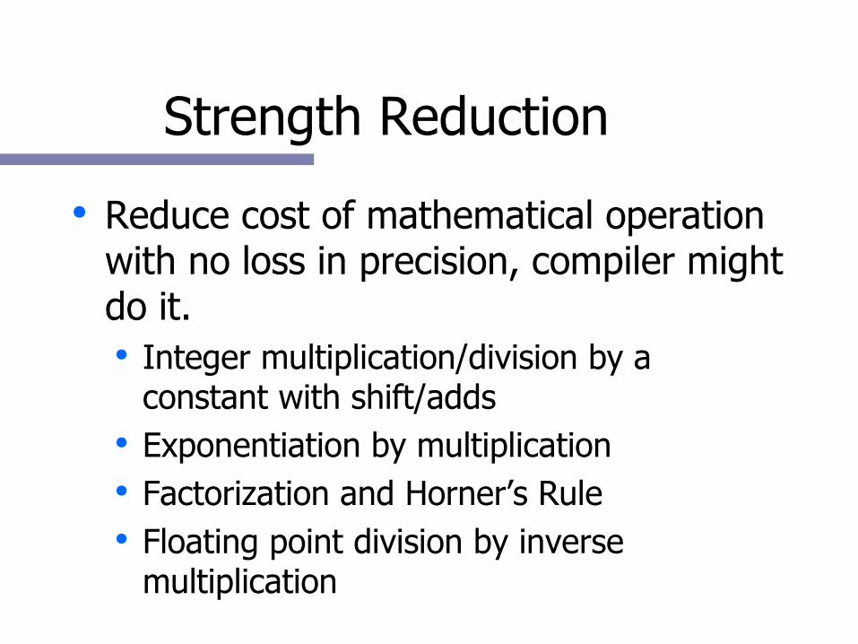
Strength Reduction
● Reduce cost of mathematical operation with no loss in precision, compiler might do it.● Integer multiplication/division by a
constant with shift/adds● Exponentiation by multiplication● Factorization and Horner’s Rule● Floating point division by inverse
multiplication

Strength ReductionHorner’s Rule
● Polynomial expression can be rewritten as a nested factorization.
Ax^5 + Bx^4 + Cx^3 + Dx^2 + Ex + F =
((((Ax + B) * x + C) * x + D) * x + E) * x + F.
● Also uses multiply-add instructions● Eases dependency analysis

Strength ReductionHorner’s Rule
Tuned-O3
Untuned-O3
Origin2000
74.20 74.09
IBM SP2 40.69 74.71
Cray T3E 61.70 160.05

Strength ReductionInteger Division by a Power of 2
● Shift requires less cycles than division.● Both dividend and divisor must both be
unsigned or positive integers.● Divides are often costly.
● Consider also multiplying times the inverse.

Strength ReductionInteger division by a Power of 2
● Untuned
IL = 0
DO I=1,ARRAY_SIZE
DO J=1,ARRAY_SIZE
IL = IL + A(J)/2
ENDDO
ILL(I) = IL
ENDDO
● Tuned
IL = 0
ILL = 0
DO I=1,ARRAY_SIZE
DO J=1,ARRAY_SIZE
IL = IL + ISHFT(A(J),-1)
ENDDO
ILL(I) = IL
ENDDO
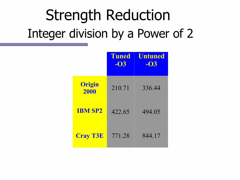
Strength Reduction Integer division by a Power of 2
Tuned-O3
Untuned-O3
Origin2000
210.71 336.44
IBM SP2 422.65 494.05
Cray T3E 771.28 844.17
Strength ReductionFactorization
● Allows for better instruction scheduling.● Compiler can interleave loads and ALU
operations.● Especially benefits compilers able to do
software pipelining.

Strength ReductionFactorization
● UntunedXX = X*A(I) + X*B(I) + X*C(I) + X*D(I)
● TunedXX = X*(A(I) + B(I) + C(I) + D(I))

Strength ReductionFactorization
Tuned-O3
Untuned-O3
Origin2000
51.65 48.99
IBM SP2 57.43 57.40
Cray T3E 387.77 443.45

Subexpression EliminationParenthesis
● Parenthesis can help the compiler recognize repeated expressions.
● Some preprocessors and aggressive compilers will do it.
● Might limit aggressive optimizations

Subexpression EliminationParenthesis
● UntunedXX = XX + X(I)*Y(I)+Z(I) + X(I)*Y(I)-Z(I) + X(I)*Y
(I) + Z(I)
● TunedXX = XX + (X(I)*Y(I)+Z(I)) + X(I)*Y(I)-Z(I) + (X
(I)*Y(I)+Z(I))

Subexpression EliminationType Considerations
● Changes the type or precision of data.● Reduces resource requirements.● Avoid type conversions.● Processor specific performance.
● Do you really need 8 or 16 bytes of precision?

Subexpression EliminationType Considerations
● Consider which elements are used together?● Should you be merging your arrays?● Should you be splitting your loops for
better locality?● For C, are your structures packed tightly in
terms of storage and reference pattern?

F90 Considerations
● WHERE statements● ARRAY syntax● ALLOCATE placement● OO complication
● Class dependencies● Code fragmentation● Operator overloading● Inlining
F90 WHERE
● This construct is basically a masking operator for array operations.
● It results in an IF statement for every operation.
● Consider copying to temporary and then multiplying by mask array.

F90 ARRAY
● Be aware that specifying sections of arrays often implies a copy.
● Often this is done more than once in your code.
● Consider doing it yourself and saving the result for reuse.

F90 ALLOCATE
● Recent experiments have shown that ALLOCATE often returns data on a page boundary.
● Very dangerous for caches with low associativity.

C/C++ Considerations
● Use STL and the C++ operators.● Dynamic typing and polymorphism isn't
free.● Use inline, const and restrict
keywords.● Easy to become memory/pointer bound
with operator overloading.● OO complication as before.

STL and C++
● The goal of STL is to export more of the author's intent to the compiler.
● Many classes run much faster than handwritten code in applications● Strong typing● The compiler can tell what you're doing vs.
just making a function call on a pointer.

Parallel Optimization

Parallel Performance
“The single most important impediment to good parallel
performance is still poor single-node performance.”
- William GroppArgonne National Lab
What is Good Parallel Performance?
● Single CPU performance is high.● The code is scalable out to more than a
few nodes.● The network is not the bottleneck.● In parallel computation, algorithm design
is the key to good performance. ● You must reduce the amount of data
that needs to be sent around.

Beware The FallacyLinear Scalability
● But what about per/PE performance?● With a slow code, overall performance of
the code is not vulnerable to other system parameters like communication bandwidth, latency.
● Very common on tightly integrated systems where you can simple add PE's for performance.
Parallel Optimization
● Two programming models.● Message Passing● Shared Memory

Parallel Performance
● Architecture is characterized by● Number of CPU’s● Connectivity● I/O capability● Single processor performance
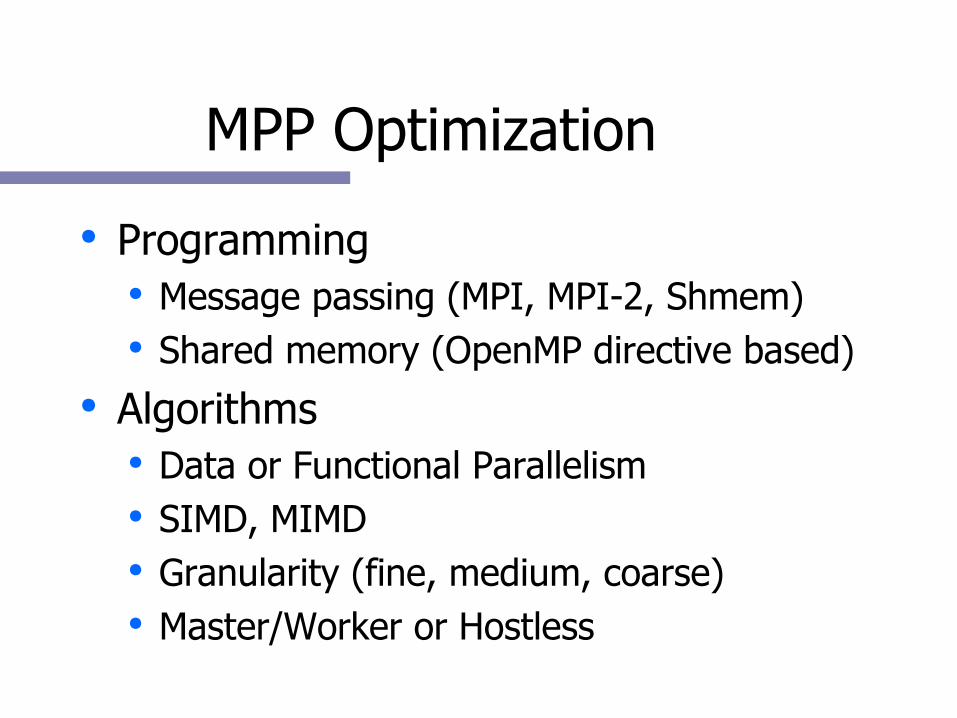
MPP Optimization
● Programming● Message passing (MPI, MPI-2, Shmem)● Shared memory (OpenMP directive based)
● Algorithms● Data or Functional Parallelism● SIMD, MIMD● Granularity (fine, medium, coarse)● Master/Worker or Hostless
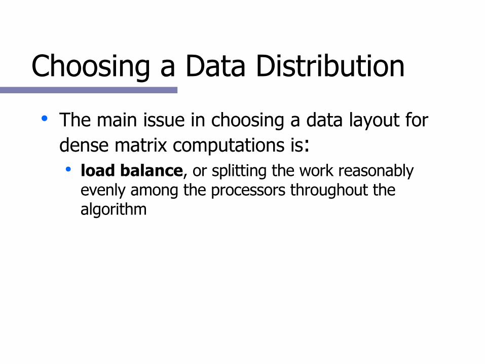
Choosing a Data Distribution
● The main issue in choosing a data layout for dense matrix computations is:● load balance, or splitting the work reasonably
evenly among the processors throughout the algorithm

Possible Data Layouts● 1D block and cyclic column distributions
● 1D block-cyclic column and 2D block-cyclic distribution used in ScaLAPACK

Two-dimensional Block-Cyclic Distribution
● Ensure good load balance --> Performance and scalability,
● Encompasses a large number of (but not all) data distribution schemes,
● Need redistribution routines to go from one distribution to the other.
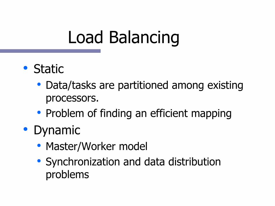
Load Balancing
● Static● Data/tasks are partitioned among existing
processors.● Problem of finding an efficient mapping
● Dynamic● Master/Worker model● Synchronization and data distribution
problems

Traditional Message Passing
● Node 1 needs X bytes from node 0● Node 0 calls a send function (X bytes
from address A)● Node 1 calls a receive function (X bytes
into address B)

Remote DMA
● Node 1 needs X bytes to addr. A from node 0 at addr. B
● Either:● Node 0 sends RDMA PUT (X bytes from
addr. A to Node 1 addr. B)● Node 1 sends RDMA GET to Node 0 (X
bytes from addr. A to Node 1 addr. B)

Memory Window's
● Node 0: Declare comm. region between addr. A and B.
● Node 1: Declare comm. region between addr. C and D.
● Either node issues a PUT or GET.

MPI Optimization

Communication Issues
● Startup time, latency or overhead● Bandwidth● Network contention and congestion● Bidirectionality● Communication API● Dedicated Channels

Communication Issues
● Startup time and bandwidth● Startup time is higher than the time to
actually transfer a small message.● Send larger messages fewer times, but try
to keep everyone busy.● Contention can be reduced by uniformly
distributing messages.

Message Passing Interface
● Provides numerous send/recv modes.● Asynchronous● One-sided
● Provides optimized collective operations.
● Supports customized data types.● Is a standard and is highly portable.

Message Passing
● Upon message arrival● If node B has not posted a receive the
data is buffered until the receive function is called.
● Else the data is delivered directly to the address given to the receive function. No copy!
● The amount of buffering is implementation dependent.

Posting a Receive
● Means that the application has informed the communication layer about a message to be received (soon).
● Matching done in software, not hardware:● context, rank and tag.
● User should provide as much information as possible to MPI to reduce matching operation.

MPI Protocol
● Often 2 or 3 message size ranges.● Short messages:
● Send right away, buffer, match and copy at receiver.
● Medium messages.● Send first chunk, ask for more space or
match, return with dest. addr. or wait.● Long
● Send first chunk, return with dest. addr.
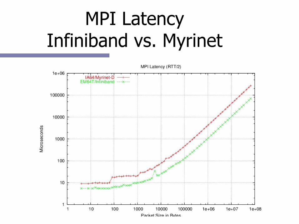
MPI LatencyInfiniband vs. Myrinet

MPI Bidirectional BandwidthInfiniband vs. Myrinet

Message Passing
● It is possible for sends and receives to be● Nonblocking(send) or Posted(receive)● Synchronous(send)● Buffered● Blocking

Message Passing
Buffering - Temporary storage of data. Posting - Temporary storage of an address.Nonblocking - Refers to an function A that
initiates an operation B and returns to the caller before the completion of B.
Blocking - The function A does not return to the caller until the completion of operation B.
Polling/Waiting - Testing for the completion of a nonblocking operation.

MPI Message Passing
● MPI introduces communication modes dictating semantics of completion of send operations.● Buffered - When transmitted or buffered,
space provided/limited by application, else error.
● Ready - Only if receive is posted, else error.
● Synchronous - Only when receive begins to execute, else wait. Useful for debugging.

MPI Message Passing
● In additionstandard - MPI will decide if/how much
outgoing data is buffered. If space is unavailable, completion will be delayed until data is transmitted to receiver. (Like PVM)
Immediate - nonblocking, returns to the caller ASAP. May be used with any of the above modes.

MPI Message Passing
● Ready sends can remove a handshake for large messages.
● There is only one receive mode, it matches any of the send modes.

MPI Optimizations
● We are primarily interested inMPI_ISEND, MPI_IRECV, MPI_IRSEND
● Why? Because your program could be doing something useful while sending or receiving! You can hide much of the cost of these communication operations.
MPI Message Passing
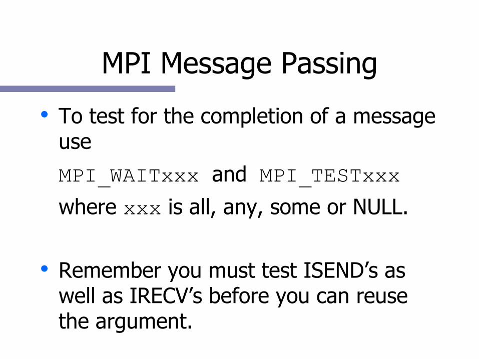
● To test for the completion of a message use
MPI_WAITxxx and MPI_TESTxxx
where xxx is all, any, some or NULL.
● Remember you must test ISEND’s as well as IRECV’s before you can reuse the argument.
MPI Data Types
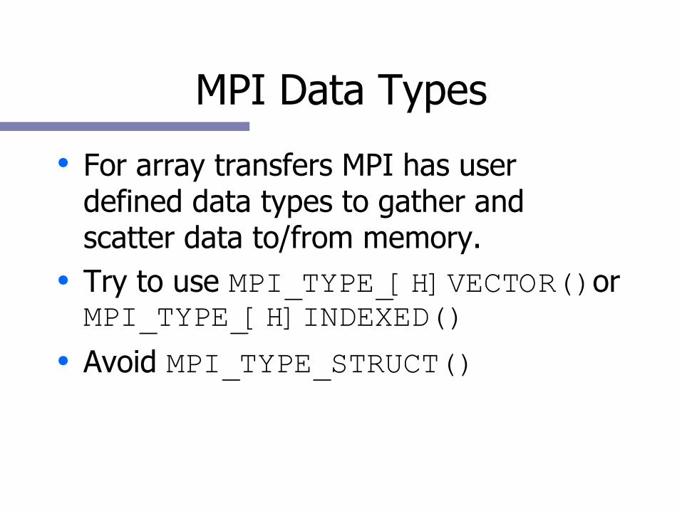
● For array transfers MPI has user defined data types to gather and scatter data to/from memory.
● Try to use MPI_TYPE_[H]VECTOR()or MPI_TYPE_[H]INDEXED()
● Avoid MPI_TYPE_STRUCT()

MPI Performance Tips
● Send big messages, infrequently.● Avoid, small frequent messages.● Think about the actual communication
pattern.● Use a collective operation.
MPI Performance Tips
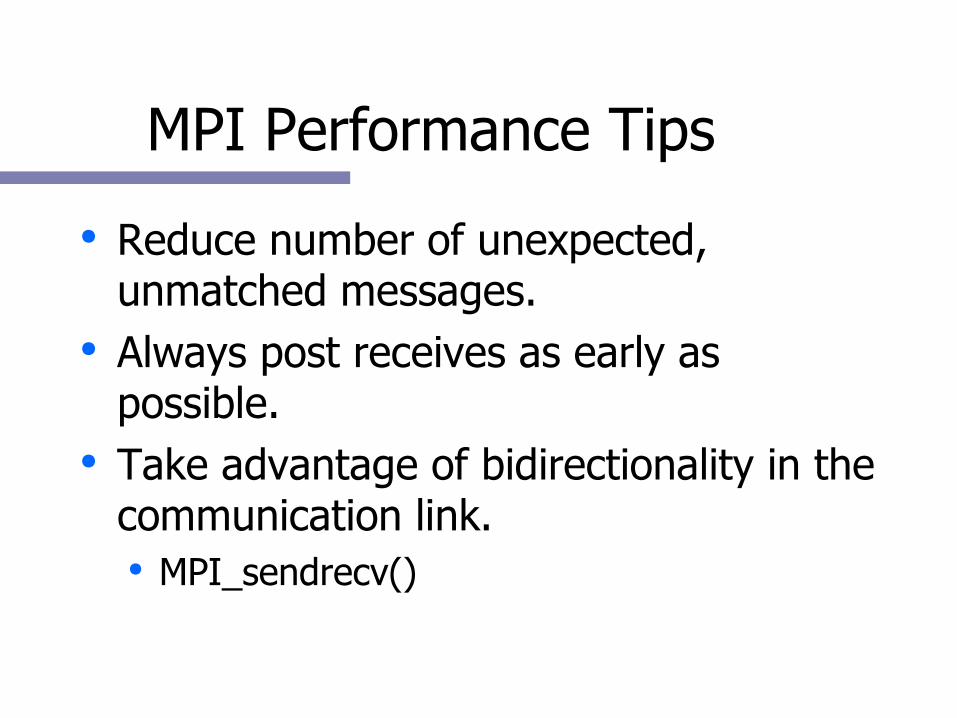
● Reduce number of unexpected, unmatched messages.
● Always post receives as early as possible.
● Take advantage of bidirectionality in the communication link.● MPI_sendrecv()

MPI Performance Tips
● Avoid data translation and derived data types unless necessary for good performance.
● Avoid wildcard receives.● Align application buffers to double
words and page sizes.
MPI Performance Tips
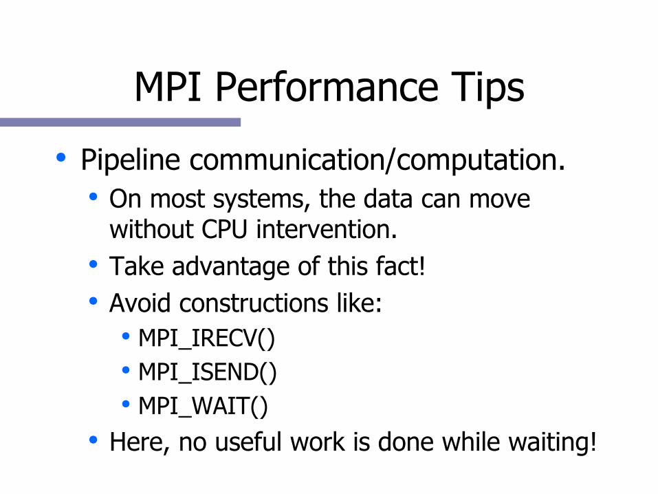
● Pipeline communication/computation.● On most systems, the data can move
without CPU intervention.● Take advantage of this fact!● Avoid constructions like:
● MPI_IRECV()● MPI_ISEND()● MPI_WAIT()
● Here, no useful work is done while waiting!

MPI Collective Communication
● Unlike PVM, with MPI you should use the collective operations. They are likely to be highly tuned for the architecture.
● These operations are very difficult to optimize and are often the bottlenecks in parallel applications.
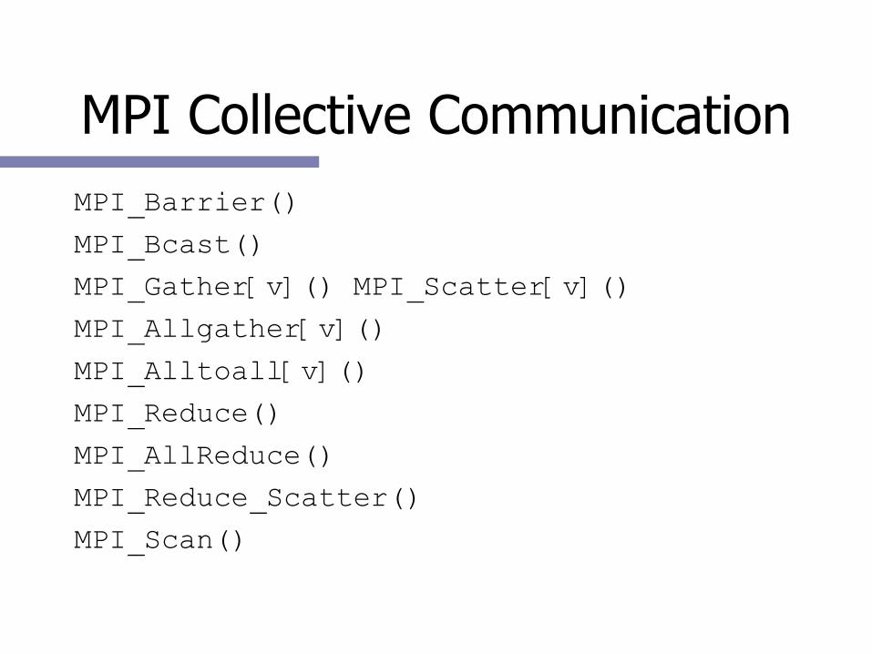
MPI Collective CommunicationMPI_Barrier()
MPI_Bcast()
MPI_Gather[v]() MPI_Scatter[v]()
MPI_Allgather[v]()
MPI_Alltoall[v]()
MPI_Reduce()
MPI_AllReduce()
MPI_Reduce_Scatter()
MPI_Scan()

Message Passing OptimizationNearest Neighbor Example 1
N slave processors available plus Master, M particles each having (x,y,z) coordinates.
1) Master reads and distributes all coordinates to N processors.
2) Each processor calculates its subset of M/N and sends it back to the master.
3) Master processor receives and outputs information.

Message Passing OptimizationNearest Neighbor Example 2
1) Master reads and scatters M/N coordinates to N processors.
2) Each processor receives its own subset and makes a replica.
3) Each processor calculates its subset of M/N coordinates versus the replica.
4) Each processor sends to the next processor its replica of M/N coordinates.
5) Each processor receives the replica. Goto 3) N-1 times.
6) Each processor sends its info back to the Master
Message Passing OptimizationNearest Neighbor Example
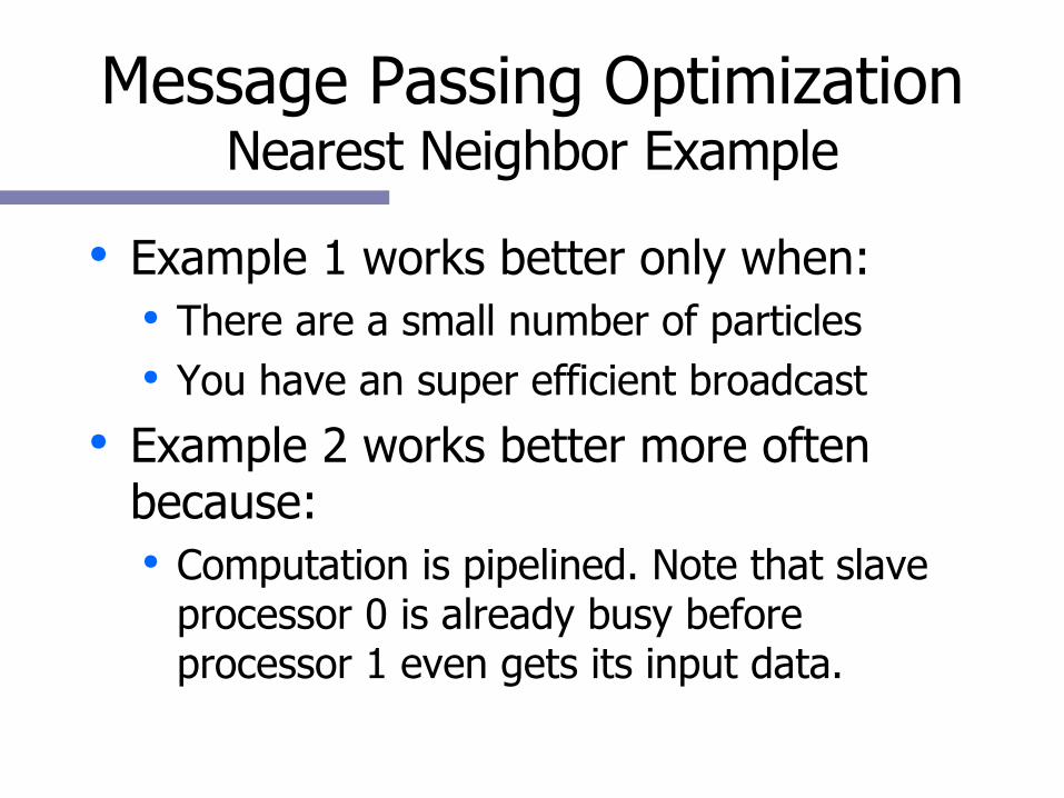
● Example 1 works better only when:● There are a small number of particles● You have an super efficient broadcast
● Example 2 works better more often because:● Computation is pipelined. Note that slave
processor 0 is already busy before processor 1 even gets its input data.

OpenMP Optimization

Thread Level Parallelism
● Data parallelism: different processors running the same code on different data. (SPMD)
● Task parallelism means different processors are running different procedures. (MPMD)
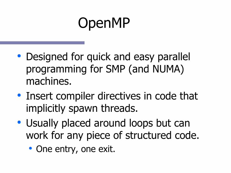
OpenMP
● Designed for quick and easy parallel programming for SMP (and NUMA) machines.
● Insert compiler directives in code that implicitly spawn threads.
● Usually placed around loops but can work for any piece of structured code.● One entry, one exit.
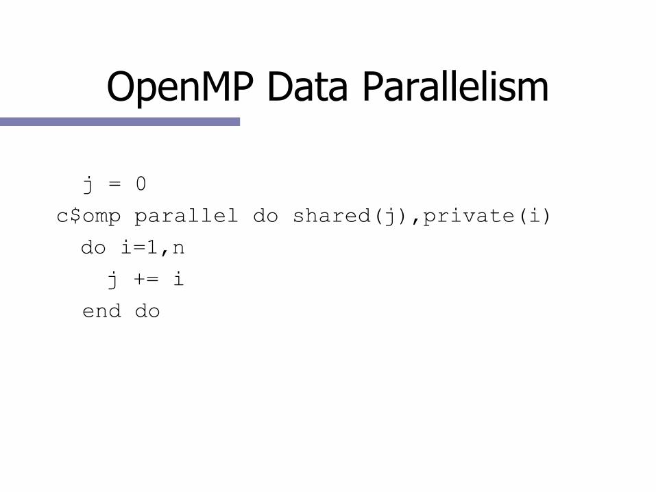
OpenMP Data Parallelism
j = 0
c$omp parallel do shared(j),private(i)
do i=1,n
j += i
end do
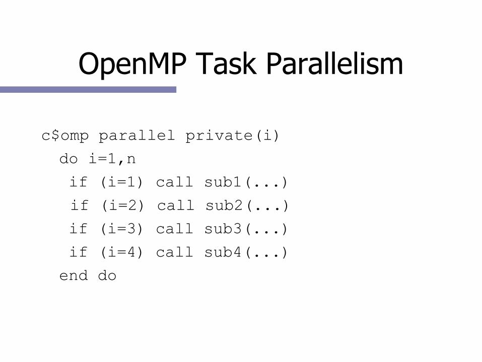
OpenMP Task Parallelism
c$omp parallel private(i)
do i=1,n
if (i=1) call sub1(...)
if (i=2) call sub2(...)
if (i=3) call sub3(...)
if (i=4) call sub4(...)
end do

Parallel Overhead
● Creating/Scheduling threads● Communication● Synchronization● Partitioning

Parallel Overhead
● For data parallel programming we can estimate some of the parallel overhead.
● Time the code with only one thread● OMP_NUM_THREADS environment
variable.● Compare with code compiled without
OpenMP turned on.

Reducing Parallel Overhead
● Don’t parallelize ALL the loops.● Parallelize the big loops.● Privatize variables where possible
● Create per thread temporaries with● PRIVATE, FIRSTPRIVATE, THREADPRIVATE

Reducing Parallel Overhead
● Use task parallelism.● Lower overhead● More code runs in parallel● Requires a parallel algorithm

Improving Load Balance
● Change the way loop iterations are allocated to threads.● Change the scheduling type● Change the chunk size
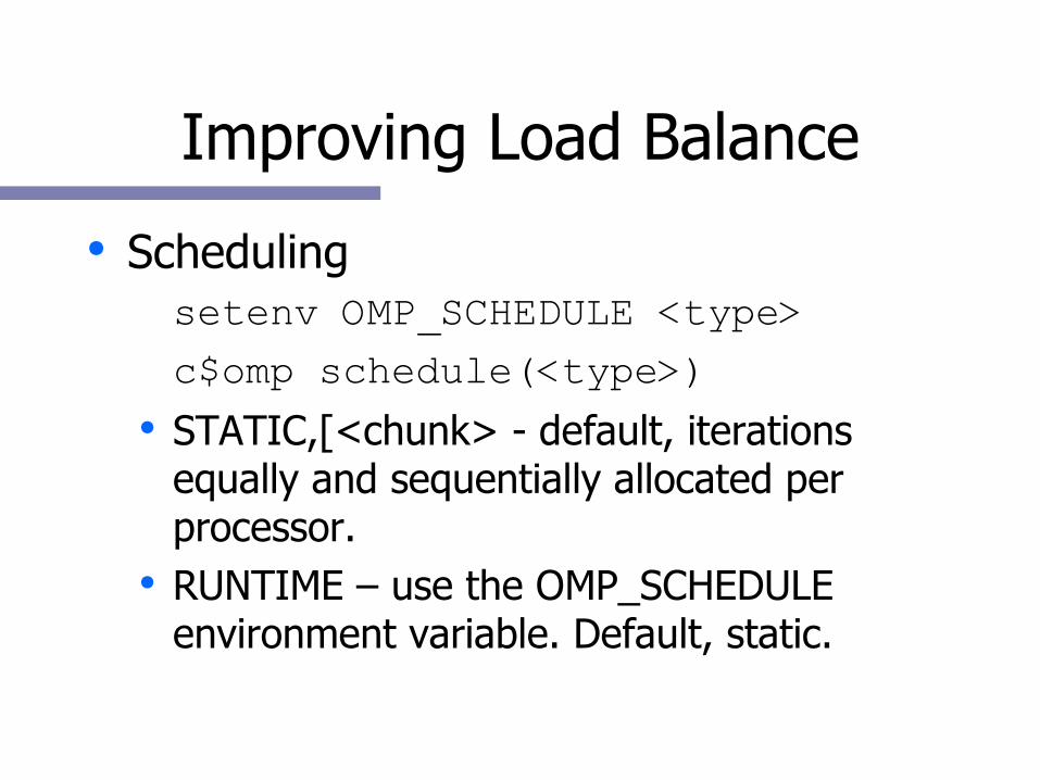
Improving Load Balance
● Scheduling – setenv OMP_SCHEDULE <type>
– c$omp schedule(<type>)● STATIC,[<chunk> - default, iterations
equally and sequentially allocated per processor.
● RUNTIME – use the OMP_SCHEDULE environment variable. Default, static.

Improving Load Balance
● Scheduling ● DYNAMIC,[<chunk>] - iterations are
allocated per processor during run-time. When the amount of work is unknown.
● GUIDED,[<chunk>] - guided self scheduling. Each processor starts with a large number and finishes with a small number.

OpenMP Gotcha's
● False sharing● Shared variables that ping-pong between
processors cache lines● Hyperthreading
● Conflicting over shared resources● OMP_NUM_THREADS to physical number
of CPU's if doing data-parallel.● Locking

Automatic Parallelization
● Let the compiler do the work.● Advantages
● It’s easy● Disadvantages
● Only does loop level parallelism.● It wants to parallelize every loop iteration
in your code.

Numerical Libraries

Optimized Arithmetic Libraries
● Advantages:● Subroutines are quick to code and
understand.● Routines provide portability.● Routines perform well.● Comprehensive set of routines.
● Disadvantages● Can lead to vertical code structure● May mask memory performance problems
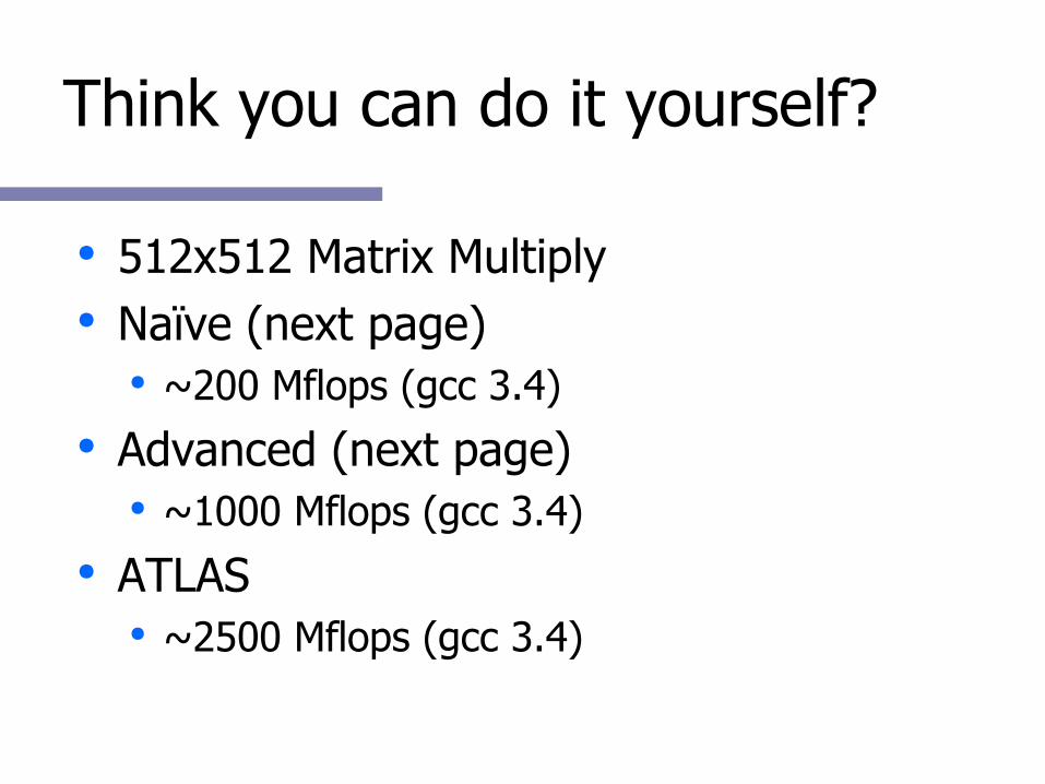
Think you can do it yourself?
● 512x512 Matrix Multiply● Naïve (next page)
● ~200 Mflops (gcc 3.4)● Advanced (next page)
● ~1000 Mflops (gcc 3.4)● ATLAS
● ~2500 Mflops (gcc 3.4)
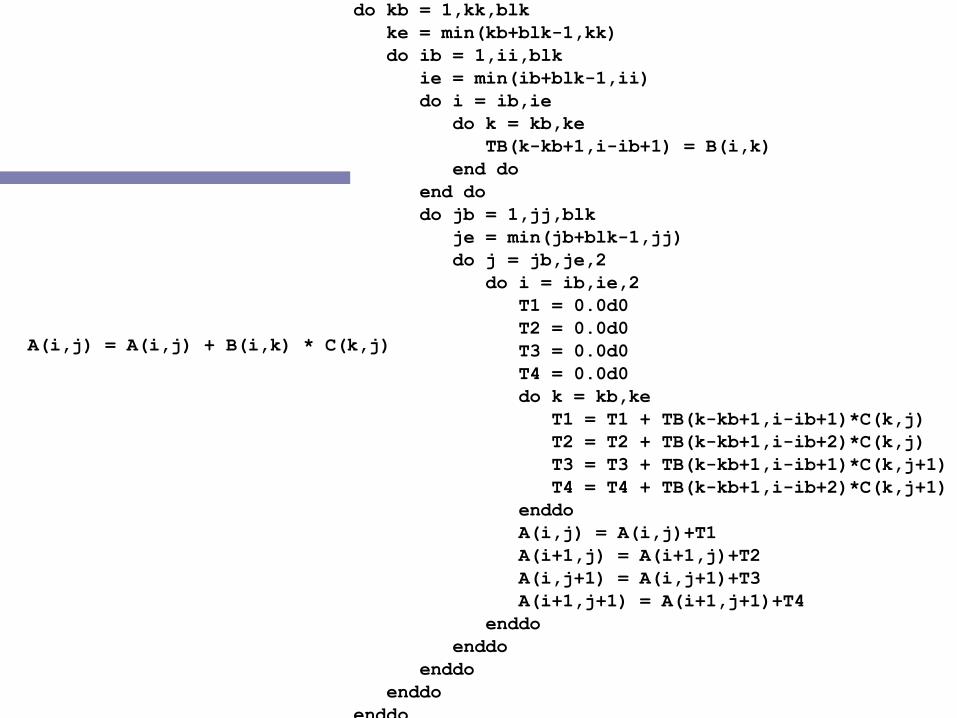
do kb = 1,kk,blk ke = min(kb+blk-1,kk) do ib = 1,ii,blk ie = min(ib+blk-1,ii) do i = ib,ie do k = kb,ke TB(k-kb+1,i-ib+1) = B(i,k) end do end do do jb = 1,jj,blk je = min(jb+blk-1,jj) do j = jb,je,2 do i = ib,ie,2 T1 = 0.0d0 T2 = 0.0d0 T3 = 0.0d0 T4 = 0.0d0 do k = kb,ke T1 = T1 + TB(k-kb+1,i-ib+1)*C(k,j) T2 = T2 + TB(k-kb+1,i-ib+2)*C(k,j) T3 = T3 + TB(k-kb+1,i-ib+1)*C(k,j+1) T4 = T4 + TB(k-kb+1,i-ib+2)*C(k,j+1) enddo A(i,j) = A(i,j)+T1 A(i+1,j) = A(i+1,j)+T2 A(i,j+1) = A(i,j+1)+T3 A(i+1,j+1) = A(i+1,j+1)+T4 enddo enddo enddo enddo enddo
A(i,j) = A(i,j) + B(i,k) * C(k,j)
Optimized Arithmetic Libraries
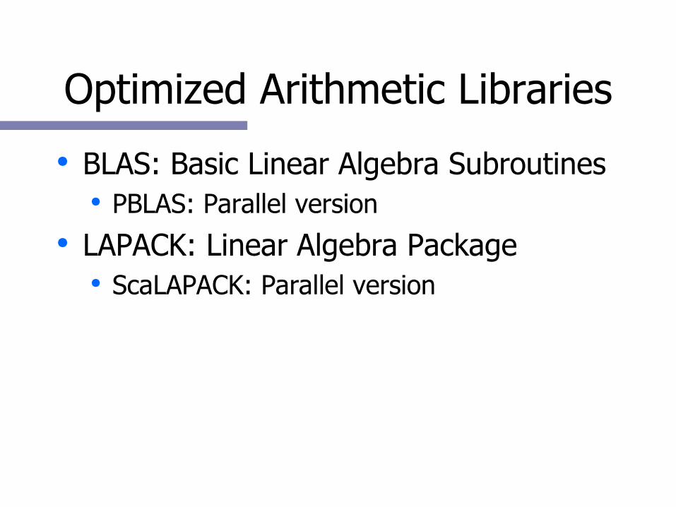
● BLAS: Basic Linear Algebra Subroutines● PBLAS: Parallel version
● LAPACK: Linear Algebra Package● ScaLAPACK: Parallel version

BLAS
● Common Matrix/Matrix, Matrix-Vector, Vector-Vector. REAL/DOUBLE/COMPLEX
● Reference version available from UT.● Vendor versions offer high
performance.● MKL on Intel● ACML on AMD
● Multithreaded are usually available.• http://www.netlib.org/blas/index.html
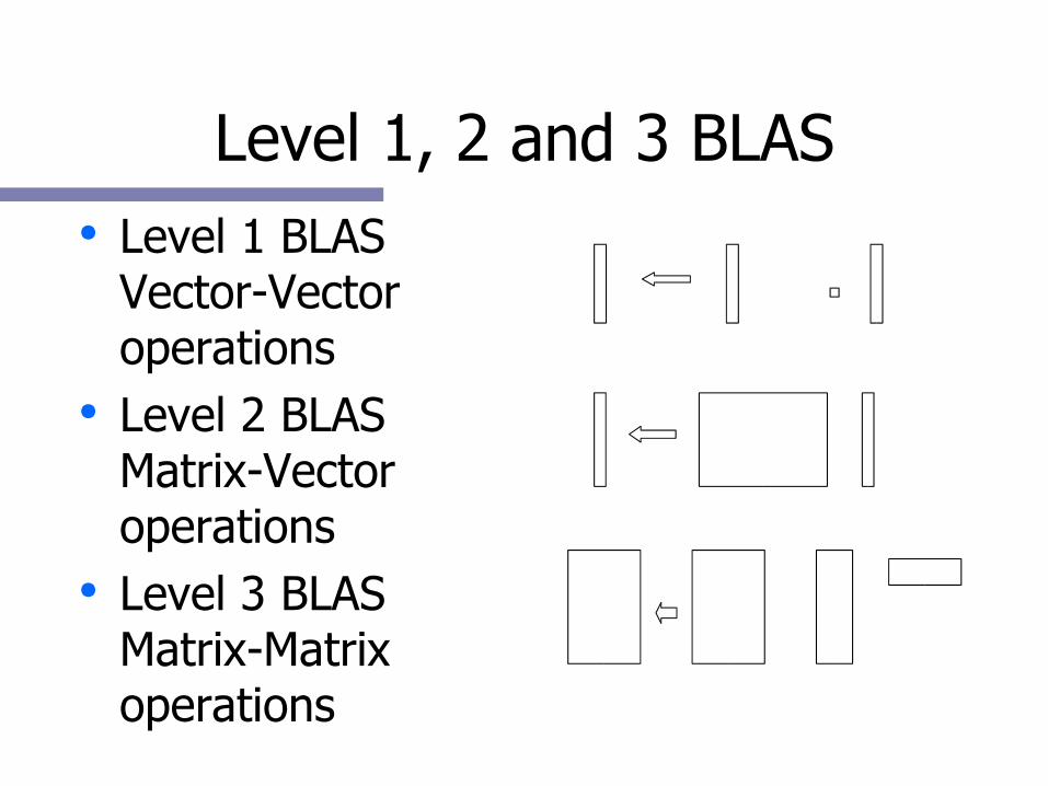
Level 1, 2 and 3 BLAS● Level 1 BLAS
Vector-Vector operations
● Level 2 BLAS Matrix-Vector operations
● Level 3 BLAS Matrix-Matrix operations
+ *
*
+ *

Goto/ATLAS BLAS
● If you don't have a vendor BLAS:● K. Goto has hand coded many BLAS
routines.● Near peak performance
● ATLAS: Automatic Tuned Linear Algebra Software● Generates near optimal BLAS and a few
LAPACK routines for ANY architecture by brute force.

LAPACK
● F77 routines for solving● systems of simultaneous linear equations
and eigenvalue problems● matrix factorizations (LU, Cholesky, QR,
SVD, Schur, generalized Schur)● Related computations such as reordering
and conditioning.● Built on the level 1, 2 3 BLAS Single,
Double, Complex, Double Complex• http://www.netlib.org/lapack/index.html

LAPACK -- Release 3.0● Add functionality
● divide and conquer SVD,● error bounds for GLM and LSE,● new expert drivers for GSEP,● faster QRP,● faster solver for the rank-deficient LS (xGELSY),● divide and conquer least squares● ...

ScaLAPACK Functionality● Orthogonal/unitary transformation routines● Prototypes
● Packed Storage routines for LLT, SEP, GSEP● Out-of-Core Linear Solvers for LU, LLT, and QR● Matrix Sign Function for Eigenproblems● SuperLU and SuperLU_MT● HPF Interface to ScaLAPACK

ScaLAPACK Documentation
● Documentation● ScaLAPACK Users’ Guide
http://www.netlib.org/scalapack/slug/scalapack_slug.html
● Installation Guide for ScaLAPACK● LAPACK Working Notes
● Test Suites for ScaLAPACK, PBLAS, BLACS
● Example Programs http://www.netlib.org/scalapack/examples/
● Prebuilt ScaLAPACK libraries on netlib
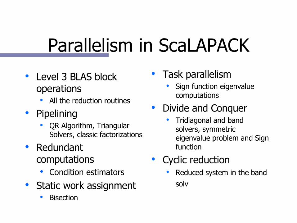
Parallelism in ScaLAPACK● Level 3 BLAS block
operations● All the reduction routines
● Pipelining● QR Algorithm, Triangular
Solvers, classic factorizations● Redundant
computations● Condition estimators
● Static work assignment● Bisection
● Task parallelism● Sign function eigenvalue
computations● Divide and Conquer
● Tridiagonal and band solvers, symmetric eigenvalue problem and Sign function
● Cyclic reduction● Reduced system in the band
solver

Narrow Band and Tridiagonal Matrices
● The ScaLAPACK routines solving narrow-band and tridiagonal linear systems assume● the narrow band or tridiagonal coefficient matrix to
be distributed in a block-column fashion, and● the dense matrix of right-hand-side vectors to be
distributed in a block-row fashion.● Divide-and-conquer algorithms have been
implemented because they offer greater scope for exploiting parallelism than the corresponding adapted dense algorithms.

PETSc
● Generalized sparse solver package for solution of PDEs.
● Multiple preconditioners and explicit and implicit methods.
● Highly optimized for compressed block storage.
● Serial and Parallel versions.
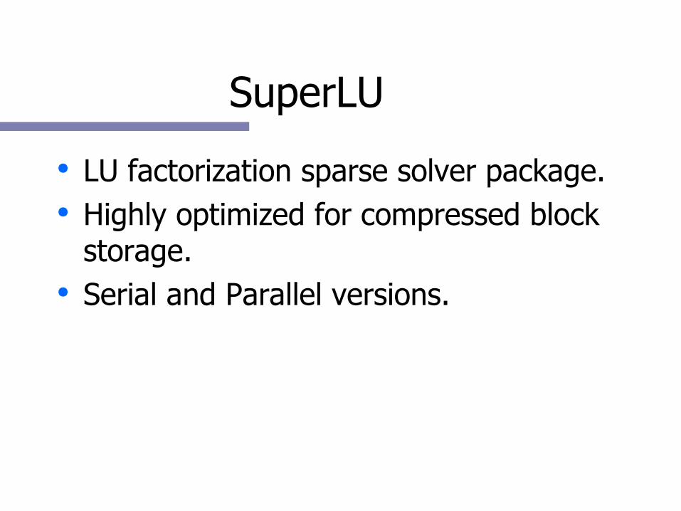
SuperLU
● LU factorization sparse solver package.● Highly optimized for compressed block
storage.● Serial and Parallel versions.

FFTW and UHFFT
● 1,2,3D FFT's on a variety of data types.● Very good performance.● Serial and Parallel versions.
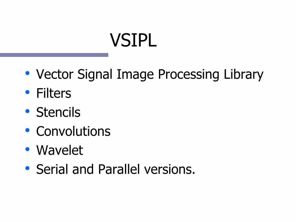
VSIPL
● Vector Signal Image Processing Library● Filters● Stencils● Convolutions● Wavelet● Serial and Parallel versions.

EISPACK
● LAPACK for Eigenvalue problems● Serial and Parallel versions.
Performance Analysis Tools
Performance Evaluation
● Traditionally, performance evaluation has been somewhat of an art form:● Limited set of tools (time & -p/-pg)● Major differences between systems● Lots of guesswork as to what was 'behind the
numbers'● Today, the situation is different.
● Hardware support for performance analysis● A wide variety of Open Source tools to
choose from.

Why Performance Analysis?● 2 reasons: Economic & Qualitative● Economic: TIME IS MONEY
● Average lifetime of these large machines is 4 years before being decommissioned.
● Consider the cost per day of a 4 Million Dollar machine, with annual maintenance/electricity cost of $300,000 (US). That's $1500.00 (US) per hour of compute time.
Why Performance Analysis 2?
● Qualitative Improvements in Science● Consider: Poorly written code can easily run
10 times worse than an optimized version.● Consider a 2-dimension domain
decomposition of a Finite Difference formulation simulation.
● For the same amount of time, the code can do 10 times the work. 400x400 elements vs. 1300x1300 elements
● Or it can do 400x400 for 10 times more time-steps.

Why Performance Analysis 3?
● So, we must strive to evaluate how our code is running.
● Learn to think of performance during the entire cycle of your design and implementation.

Processor Complexity
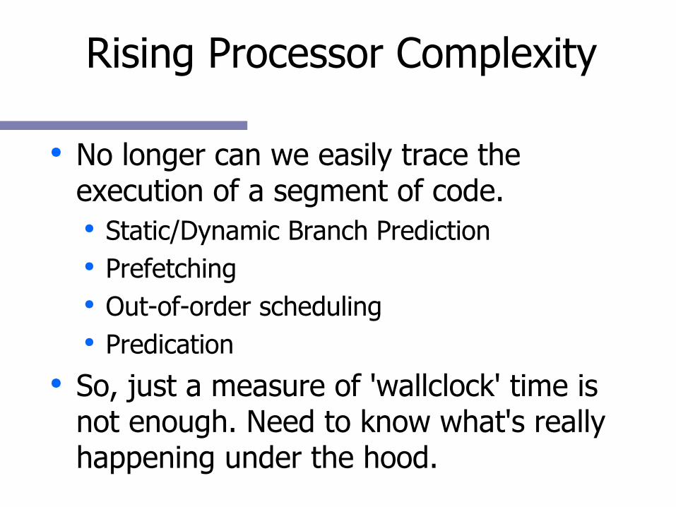
Rising Processor Complexity
● No longer can we easily trace the execution of a segment of code.● Static/Dynamic Branch Prediction● Prefetching● Out-of-order scheduling● Predication
● So, just a measure of 'wallclock' time is not enough. Need to know what's really happening under the hood.

Direct Measurement Methods● Instrumentation based
● Tracing● Generate a record for each measured event.● Useful only when evidence of performance
anomalies is present due to the large volume of data generated.
● Aggregate● Reduce data at run-time avg/min/max
measurements.● Useful for application and architecture
characterization and optimization.

Measurement Methods 2
● Indirect methods requires no instrumentation and can be used on unmodified applications.
● The reality is that the boundary between indirect and direct is somewhat fuzzy.● gprof (no source mods, but requires relink or
recompile)

Statistical Profiling
● At a defined interval (interrupts), record WHERE in the program the CPU is.
● Data gathered represents a probabilistic distribution in the form of a histogram.
● Interrupts can be based on time or hardware counter events with the proper infrastructure like...

External Timers
● /usr/bin/time <command> returns 3 kinds.● Real time: Time from start to finish● User: CPU time spent executing your code● System: CPU time spent executing system
calls ● Warning! The definition of CPU time is
different on different machines.

External Timers
● Sample output (from Linux)0.56user 0.12system 0:03.80elapsed 18%CPU
(0avgtext+0avgdata 0maxresident)k
0inputs+0outputs (55major+2684minor)pagefaults 0swaps
1) User 2) System 3) Real 4) Percent of time spent on behalf of this process, not including
waiting.5) Text size, data size, max memory6) 0 input, 0 output operations7) Page faults (major, minor), swaps.

Internal Timers
● gettimeofday(), part of the C library obtains seconds and microseconds since Jan 1, 1970.
● second(), Fortran 90.● Latency is not the same as resolution.
● Many calls to this function will affect your wall clock time.

Internal Timers
● clock_gettime() for POSIX, usually implemented as gettimeofday().
● MPI_Wtime() returns elapsed wall clock time in seconds as a double.

Hardware Performance Counters
● On/off chip registers that count hardware events
● Many different events.● OS accumulates counts into 64-bit
quantities.● Both user and kernel modes can be
measured.● Explicit counting or statistical
histograms based on counter overflow.

Performance Counters● Most high performance processors include hardware
performance counters.● AMD Athlon and Opteron● Compaq Alpha EV Series● CRAY T3E, X1● IBM Power Series● Intel Itanium, Itanium 2, Pentium● SGI MIPS R1xK Series● Sun UltraSparc II, III, IV● IBM Blue Gene● And many others...

Performance Counters● Performance Counters are hardware registers dedicated
to counting certain types of events within the processor or system.● Usually a small number of these registers (2,4,8)● Sometimes they can count a lot of events or just a few● Symmetric or asymmetric
● Each register has an associated control register that tells it what to count and how to do it.● Interrupt on overflow● Edge detection (cycles vs. events)● User vs. kernel mode

• Cycle count• Instruction count
– All instructions– Floating point– Integer– Load/store
• Branches– Taken / not taken – Mispredictions
• Pipeline stalls due to– Memory subsystem
– Resource conflicts
• Cache– I/D cache misses for
different levels – Invalidations
• TLB – Misses– Invalidations
Some Hardware Performance Counter Events

Statistical Profiling
Location
Am
ount
Time
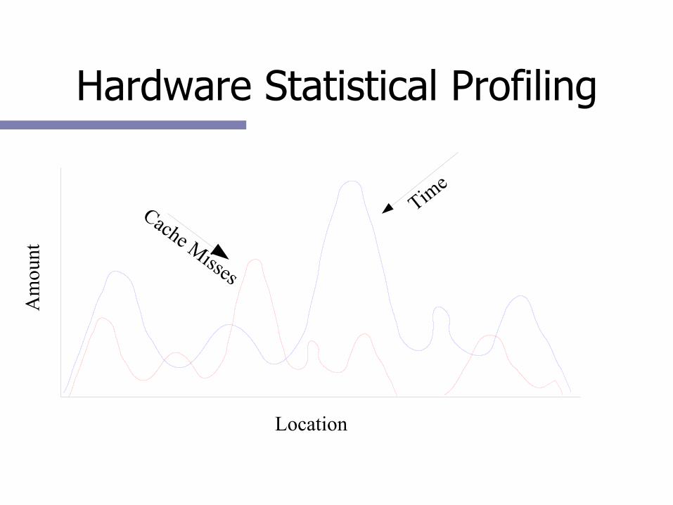
Hardware Statistical Profiling
Location
Am
ount
Time
Cache Misses

PAPI
• Performance Application Programming Interface
• The purpose of PAPI is to implement a standardized portable and efficient API to access the hardware performance monitor counters found on most modern microprocessors.
• The goal of PAPI is to facilitate the optimization of parallel and serial code performance by encouraging the development of cross-platform optimization tools.

PAPI Preset Events● PAPI supports around preset events● Proposed set of events deemed most relevant
for application performance tuning● Preset events are mappings from symbolic
names to machine specific definitions for a particular hardware resource.● Total Cycles is PAPI_TOT_CYC
● Mapped to native events on a given platform● PAPI also supports presets that may be derived
from the underlying hardware metrics

Linux Performance Tools ● Contrary to popular belief, the Linux
infrastructure is well established.● PAPI is 8 years old.● Wide complement of tools from which to
choose.● Some are production quality.● Sun, IBM and HP are now focusing on
Linux/HPC which means a focus on performance.

Which Tool?
The Right Performance Tool
● What are your needs? Things to consider:● User Interface
● Complex Suite● Quick and Dirty
● Data Collection Mechanism● Aggregate● Trace based● Statistical
The Right Performance Tool 2
● Performance Data● Communications (MPI)● Synchronization (Threads and OpenMP)● External Libraries● User code
● Data correlation● Task Parallel (MPI)● Thread Parallel
● Instrumentation Mechanism● Source/Binary/Library interposition

The Right Performance Tool 3
● Data Management● Performance Database● User (Flat file)
● Data Visualization● Run Time● Post Mortem● Serial/Parallel Display● ASCII
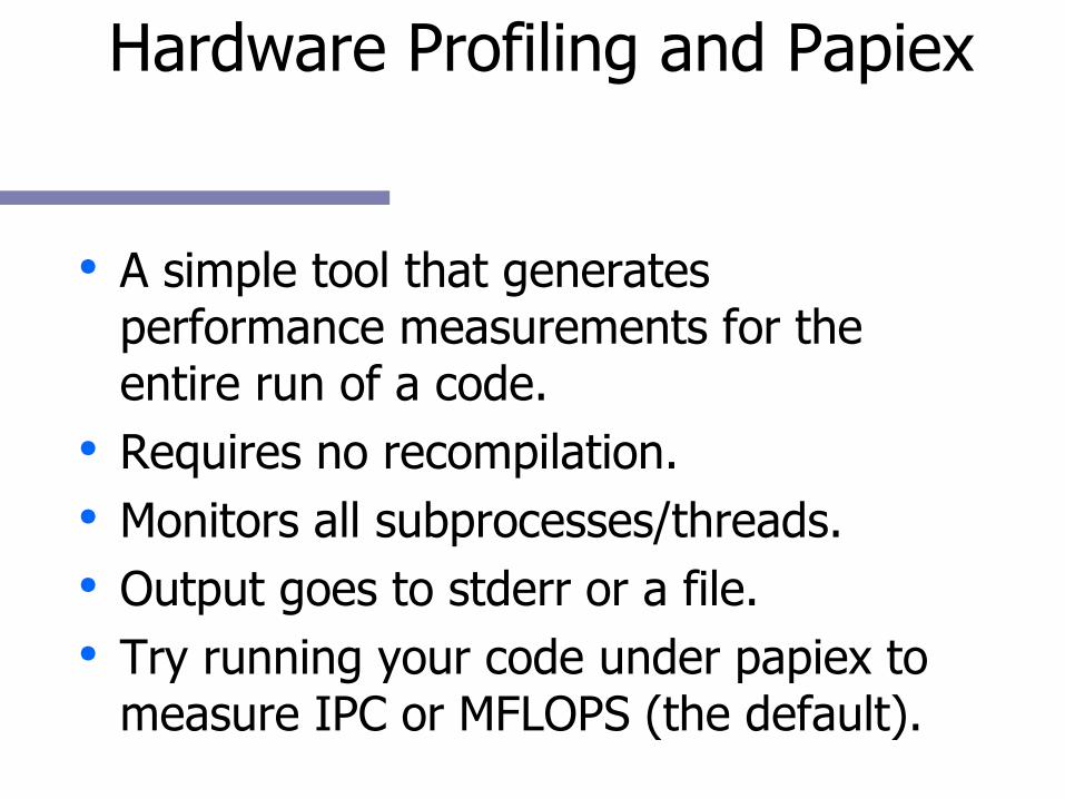
Hardware Profiling and Papiex
● A simple tool that generates performance measurements for the entire run of a code.
● Requires no recompilation.● Monitors all subprocesses/threads.● Output goes to stderr or a file.● Try running your code under papiex to
measure IPC or MFLOPS (the default).

Papiex v0.9 Example> module load perftools/1.1
> papiex <application>
> papiex -e PAPI_TOT_CYC -e PAPI_TOT_INS -- <application>
> mpirun -np 4 `which papiex` -f -- <application>
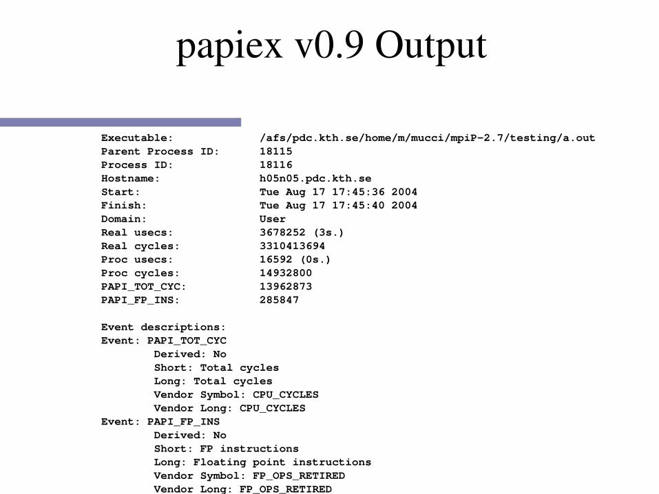
papiex v0.9 Output
Executable: /afs/pdc.kth.se/home/m/mucci/mpiP-2.7/testing/a.outParent Process ID: 18115Process ID: 18116Hostname: h05n05.pdc.kth.seStart: Tue Aug 17 17:45:36 2004Finish: Tue Aug 17 17:45:40 2004Domain: UserReal usecs: 3678252 (3s.)Real cycles: 3310413694Proc usecs: 16592 (0s.)Proc cycles: 14932800PAPI_TOT_CYC: 13962873PAPI_FP_INS: 285847 Event descriptions:Event: PAPI_TOT_CYC Derived: No Short: Total cycles Long: Total cycles Vendor Symbol: CPU_CYCLES Vendor Long: CPU_CYCLESEvent: PAPI_FP_INS Derived: No Short: FP instructions Long: Floating point instructions Vendor Symbol: FP_OPS_RETIRED Vendor Long: FP_OPS_RETIRED
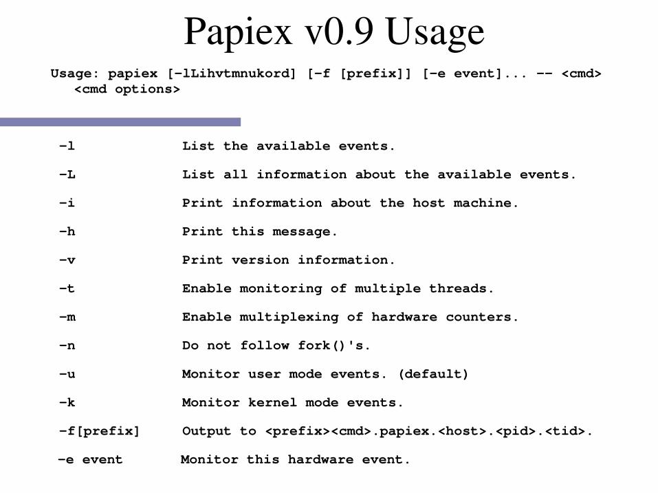
Papiex v0.9 UsageUsage: papiex [-lLihvtmnukord] [-f [prefix]] [-e event]... -- <cmd>
<cmd options>
-l List the available events.
-L List all information about the available events.
-i Print information about the host machine.
-h Print this message.
-v Print version information.
-t Enable monitoring of multiple threads.
-m Enable multiplexing of hardware counters.
-n Do not follow fork()'s.
-u Monitor user mode events. (default)
-k Monitor kernel mode events.
-f[prefix] Output to <prefix><cmd>.papiex.<host>.<pid>.<tid>.
-e event Monitor this hardware event.

Parallel Profiling
● Often we want to see how much time we are spending communicating.
● Many tools to do this via “Tracing” the MPI calls.
● A very good and simple tool available on Lucidor is mpiP v2.7, it does online trace reduction.

MpiP v2.7 Example> module load perftools/1.1
> module show perftools
● Follow the instructions to link your C/C++/F77/F90 codes with mpiP.
● Run your code and examine the output in <*.mpiP>.

MpiP v2.7 Output
@--- MPI Time (seconds) ---------------------------------------------------Task AppTime MPITime MPI% 0 0.084 0.0523 62.21 1 0.0481 0.015 31.19 2 0.087 0.0567 65.20 3 0.0495 0.0149 29.98 * 0.269 0.139 51.69
@--- Aggregate Time (top twenty, descending, milliseconds) ----------------Call Site Time App% MPI%Barrier 1 112 41.57 80.42Recv 1 26.2 9.76 18.89Allreduce 1 0.634 0.24 0.46Bcast 1 0.3 0.11 0.22Send 1 0.033 0.01 0.02
@--- Aggregate Sent Message Size (top twenty, descending, bytes) ----------Call Site Count Total Avrg Sent%Allreduce 1 8 4.8e+03 600 46.15Bcast 1 8 4.8e+03 600 46.15Send 1 2 800 400 7.69

MpiP v2.7 Output 2
@--- Callsite Time statistics (all, milliseconds): 16 Name Site Rank Count Max Mean Min App% MPI%Allreduce 1 0 2 0.105 0.087 0.069 0.21 0.33Allreduce 1 1 2 0.118 0.08 0.042 0.33 1.07Allreduce 1 2 2 0.11 0.078 0.046 0.18 0.27Allreduce 1 3 2 0.102 0.072 0.042 0.29 0.97Barrier 1 0 3 51.9 17.3 0.015 61.86 99.44...@--- Callsite Message Sent statistics (all, sent bytes) Name Site Rank Count Max Mean Min SumAllreduce 1 0 2 800 600 400 1200Allreduce 1 1 2 800 600 400 1200Allreduce 1 2 2 800 600 400 1200Allreduce 1 3 2 800 600 400 1200Bcast 1 0 2 800 600 400 1200Bcast 1 1 2 800 600 400 1200Bcast 1 2 2 800 600 400 1200Bcast 1 3 2 800 600 400 1200Send 1 0 1 400 400 400 400Send 1 2 1 400 400 400 400Send 1 * 18 800 577.8 400 1.04e+04---------------------------------------------------------------------------@--- End of Report --------------------------------------------------------

MPI Tracing and Jumpshot● Sometimes we need to see the exact
sequence of messages exchanged between processes.
● For this, we can enable MPI tracing by relinking our application and using the Jumpshot tool.
● Works with any MPI by linking with the Jumpshot MPI tracing library.
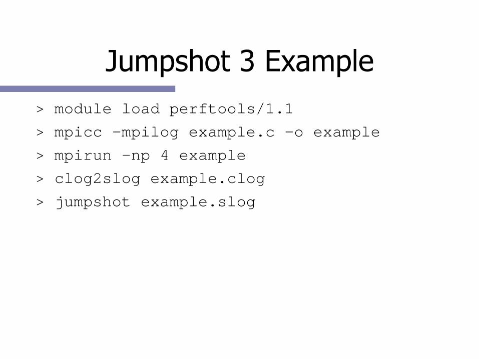
Jumpshot 3 Example> module load perftools/1.1
> mpicc -mpilog example.c -o example
> mpirun -np 4 example
> clog2slog example.clog
> jumpshot example.slog

Jumpshot Main Window

Jumpshot Timeline
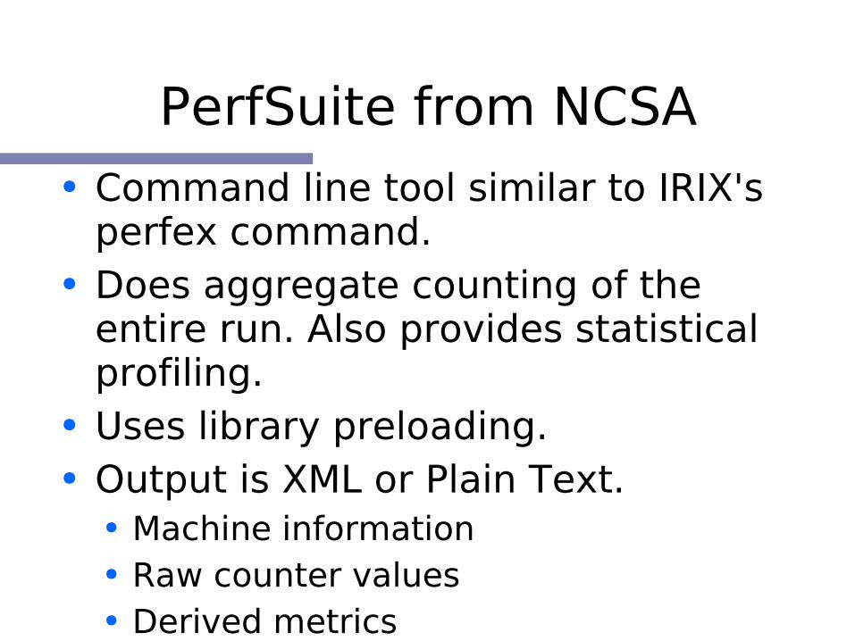
PerfSuite from NCSA● Command line tool similar to IRIX's
perfex command.● Does aggregate counting of the
entire run. Also provides statistical profiling.
● Uses library preloading.● Output is XML or Plain Text.
● Machine information● Raw counter values● Derived metrics

PSRUN Sample OutputIndex Description Counter Value============================================================================================
1 Conditional branch instructions mispredicted..................... 4831072449 2 Conditional branch instructions correctly predicted.............. 52023705122 3 Conditional branch instructions taken............................ 47366258159 4 Floating point instructions...................................... 86124489172 5 Total cycles..................................................... 594547754568 6 Instructions completed........................................... 1049339828741 7 Level 1 data cache accesses...................................... 30238866204 8 Level 1 data cache hits.......................................... 972479062 9 Level 1 data cache misses........................................ 29224377672 10 Level 1 instruction cache reads.................................. 221828591306 11 Level 1 cache misses............................................. 29312740738 12 Level 2 data cache accesses...................................... 129470315862 13 Level 2 data cache misses........................................ 15569536443 14 Level 2 data cache reads......................................... 110524791561 15 Level 2 data cache writes........................................ 18622708948 16 Level 2 instruction cache reads.................................. 566330907 17 Level 2 store misses............................................. 1208372120 18 Level 2 cache misses............................................. 15401180750 19 Level 3 data cache accesses...................................... 4650999018 20 Level 3 data cache hits.......................................... 186108211 21 Level 3 data cache misses........................................ 4451199079 22 Level 3 data cache reads......................................... 4613582451 23 Level 3 data cache writes........................................ 38456570 24 Level 3 instruction cache misses................................. 3631385 25 Level 3 instruction cache reads.................................. 17631093 26 Level 3 cache misses............................................. 4470968725 27 Load instructions................................................ 111438431677 28 Load/store instructions completed................................ 130391246662 29 Cycles Stalled Waiting for memory accesses....................... 256484777623 30 Store instructions............................................... 18840914540 31 Cycles with no instruction issue................................. 61889609525 32 Data translation lookaside buffer misses......................... 2832692

PSRUN Sample Output
Statistics============================================================================================Graduated instructions per cycle....................................... 1.765Graduated floating point instructions per cycle........................ 0.145% graduated floating point instructions of all graduated instructions.. 8.207Graduated loads/stores per cycle....................................... 0.219Graduated loads/stores per graduated floating point instruction........ 1.514Mispredicted branches per correctly predicted branch................... 0.093Level 1 data cache accesses per graduated instruction.................. 2.882Graduated floating point instructions per level 1 data cache access.... 2.848Level 1 cache line reuse (data)........................................ 3.462Level 2 cache line reuse (data)........................................ 0.877Level 3 cache line reuse (data)........................................ 2.498Level 1 cache hit rate (data).......................................... 0.776Level 2 cache hit rate (data).......................................... 0.467Level 3 cache hit rate (data).......................................... 0.714Level 1 cache miss ratio (instruction)................................. 0.003Level 1 cache miss ratio (data)........................................ 0.966Level 2 cache miss ratio (data)........................................ 0.120Level 3 cache miss ratio (data)........................................ 0.957Bandwidth used to level 1 cache (MB/s)................................. 1262.361Bandwidth used to level 2 cache (MB/s)................................. 1326.512Bandwidth used to level 3 cache (MB/s)................................. 385.087% cycles with no instruction issue..................................... 10.410% cycles stalled on memory access...................................... 43.139MFLOPS (cycles)........................................................ 115.905MFLOPS (wallclock)..................................................... 114.441MIPS (cycles).......................................................... 1412.190MIPS (wallclock)....................................................... 1394.349CPU time (seconds)..................................................... 743.058Wall clock time (seconds).............................................. 752.566% CPU utilization...................................................... 98.737

HPCToolkit from Rice U.● Use event-based sampling and statistical
profiling to profile unmodified applications: hpcrun
● Interpret program counter histograms: hpcprof
● Correlate source code, structure and performance metrics: hpcprof/hpcquick
● Explore and analyze performance databases: hpcviewer
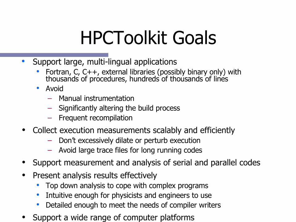
HPCToolkit Goals● Support large, multi-lingual applications
● Fortran, C, C++, external libraries (possibly binary only) with thousands of procedures, hundreds of thousands of lines
● Avoid– Manual instrumentation– Significantly altering the build process– Frequent recompilation
• Collect execution measurements scalably and efficiently– Don’t excessively dilate or perturb execution– Avoid large trace files for long running codes
• Support measurement and analysis of serial and parallel codes
• Present analysis results effectively● Top down analysis to cope with complex programs ● Intuitive enough for physicists and engineers to use● Detailed enough to meet the needs of compiler writers
• Support a wide range of computer platforms

HPCToolkit Sample Output

TAU from U. Oregon● Integrated toolkit for parallel and serial
performance instrumentation, measurement, analysis, and visualization
● Open software approach with technology integration
● Robust timing and hardware performance support using PAPI
● TAU supports both profiling and tracing models.

Some TAU Features
● Function-level, block-level, statement-level
● Support for callgraph and callpath profiling
● Parallel profiling and Inter-process communication events
● Supports user-defined events● Trace merging and format conversion
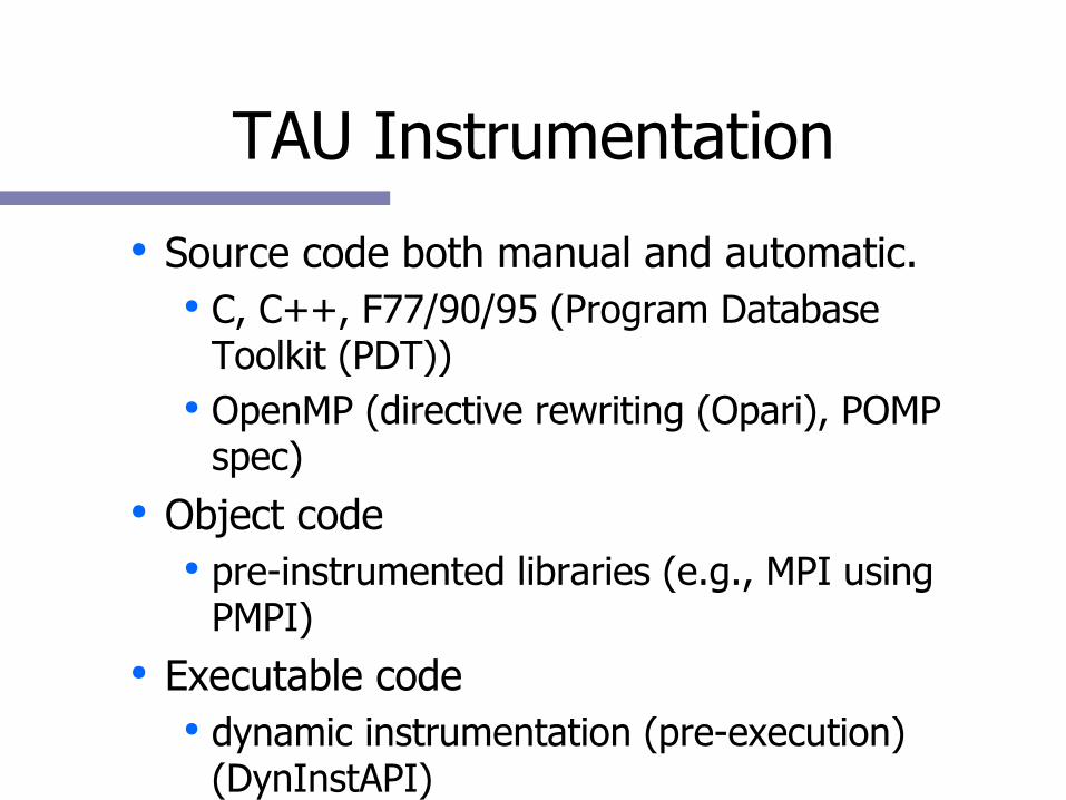
TAU Instrumentation● Source code both manual and automatic.
● C, C++, F77/90/95 (Program Database Toolkit (PDT))
● OpenMP (directive rewriting (Opari), POMP spec)
● Object code● pre-instrumented libraries (e.g., MPI using
PMPI)● Executable code
● dynamic instrumentation (pre-execution) (DynInstAPI)

TAU Parallel Display

TAU Program Display

● KOJAK (Juelich, UTK)● Instrumentation, tracing and analysis system for
MPI, OpenMP and Performance Counters.● Provides automated diagnosis of many common
parallel performance problems.● Q-Tools (HP) (non-PAPI, IA64 only)
● Statistical profiling of system and user processes● DynaProf (Me)
● Dynamic instrumentation tool.
More Performance Tools
Conclusion

5 Ways to Avoid Performance Problems: Number 1
Never, ever, write your own code unless you absolutely have to.● Libraries, libraries, libraries!● Spend time to do the research, chances are
you will find a package that suits your needs.
● Often you just need to do the glue that puts the application together.
● The 80/20 Rule! 80% of time is spent in 20% of code.

5 Ways to Avoid Performance Problems: Number 2
Never violate the usage model of your environment.● If something seems impossible to
accomplish in your language or programming environment, you're probably doing something wrong.
● Consider such anomalies as:● Matlab in parallel on a cluster of machines.● High performance(?!) Java.
● There probably is a better way to do it, ask around.

5 Ways to Avoid Performance Problems: Number 3
Always let the compiler do the work.● The compiler is much better at optimizing
most code than you are. ● Gains of 30-50% are reasonably common
when the 'right' flags are thrown.● Spend some time to read the manual and
ask around.
5 Ways to Avoid Performance Problems: Number 4
Never use more data than absolutely necessary.● C: float vs. double.● Fortran: REAL*4, REAL*8, REAL*16 ● Only use 64-bit precision if you NEED it.● A reduction in the amount of data the CPU
needs ALWAYS translates to a increase in performance.
● Remember that the memory subsystem and the network are the ultimate bottlenecks.

5 Ways to Avoid Performance Problems: Number 5
Always make friends with a computer scientist!● Learning just a little about modern computer
architecture will result in much better code.

Questions?
● Email: [email protected]● For those here at KTH, many on the PDC
staff are well versed in the art of performance. Use them!

HTTP Referenceshttp://www.openmp.org
http://www.netlib.org
http://http://www-unix.mcs.anl.gov/petsc/petsc-2/
http://crd.lbl.gov/~xiaoye/SuperLU
http://www.netlib.org/eispack
http://www2.cs.uh.edu/~mirkovic/fft/parfft.htm
http://www.fftw.org
http://www.intel.com/software/products/mkl
http://www.cs.utexas.edu/users/flame/goto
http://www.netlib.org/atlas
http://www.vsipl.org

HTTP Referenceshttp://www.cs.utk.edu/~mucci/latest/mucci_talks.html
http://icl.cs.utk.edu/papi
http://www.fz-juelich.de/zam/kojak/
http://www.hpl.hp.com/research/linux/q-tools
http://www.cs.utk.edu/~mucci/papiex
http://www.cs.utk.edu/~mucci/dynaprof
http://www.cs.uoregon.edu/research/paracomp/tau/
http://hipersoft.cs.rice.edu/hpctoolkit/
http://perfsuite.ncsa.uiuc.edu
http://www.cs.utk.edu/~mucci/MPPopt.html
Thanks