Performance Measures for Rural Transportation … Measures for Rural Transportation Systems...

Performance Measures for

Rural Transportation Systems GUIDEBOOK

JUNE 2006

Contents Introduction… … … … … … … … … … … … … … … … … … … … … … … … … … … … … … … … … … … i Section 1 - Safety… … … … … … … … … … … … … … … … … … … … … … … … … … .… … … 1-1

Introduction and Definition… … … … … … … … … … … … … … … … … … … … … … … … … ....… 1-1 How Would a Rural Area Measure Safety?....................................................................... 1-1 Step-by-Step Guidance – Basic...… … … … … … … … … … … … … … … … … ...… … … … … … 1-1 Quick Reference – Safety… … … … … … … … … … … … … … … … … … … … … … … … … … … . 1-5

Section 2 - System Preservation… … … … … … … … … … … … … … … … … … … ..… … … … . 2-1 Introduction and Definition… … … … … … … … … … … … … … … … … … … … … … … … … ..… .. 2-1 How Would a Rural Area Measure System Preservation? … … … … … … … … … … … … … . 2-2 Step-By-Step Guidance – Basic… … … … … … … … … … … … … … … … … … … … ...… .......... 2-3 Step-By-Step Guidance – Intermediate… … … … … … … … … … … … … … … … … … … … ..... 2-6 Step-By-Step Guidance – Advanced… … … … … … … … … … … … … … … … … … … … ...… .. 2-13 Quick Reference – System Preservation… … … … … … … … … … … … … … … … … … … … … 2-15

Section 3 - Mobility… … … … … … … … … … … … … … … … … … … … … … … .… … … … … … … … 3-1 Introduction and Definition… … … … … … … … … … … … … … … … … … … … … … … … … … … 3-1 How Would a Rural Area Measure Mobility? … … … … … … … … … … … … … … … … … … … 3-2 Step-by-Step Guidance – Basic… … … … … … … … … … … … … … … … … … … … … … … … .. 3-3 Step-By-Step Guidance – Intermediate… … … … … … … … … … … … … … … … … … … … ..... 3-5 Step-By-Step Guidance – Advanced… … … … … … … … … … … … … … … … … … … … … ...... 3-6 Quick Reference – Mobility… … … … … … … … … … … … … … … … … … … … … … … … … … .. 3-9

Section 4 - Accessibility… … … … … … … … … … .… … … … … … … … … … … … … … … .. 4-1 Introduction and Definition… … … … … … … … … … … … … … … … … … … … … … … … … … … . 4-1 How Would a Rural Area Measure Accessibility? … … … … … … … … … … … … … … … … … 4-1 Step-by-Step Guidance – Basic… … … … … … … … … … … … … … … … … … … … … … … … .. 4-3 Step-By-Step Guidance – Intermediate… … … … … … … … … … … … … … … … … … … … ..... 4-3 Step-By-Step Guidance – Advanced… … … … … … … … … … … … … … … … … … … … … ...... 4-6 Quick Reference – Accessibility… … … … … … … … … … … … … … … … … … … … … … … … .. 4-7

Section 5 - Reliability… … … … … … … … … … .… … … … … … … … … … … … … … … … … … ....... 5-1 Introduction and Definition… … … … … … … … … … … … … … … … … … … … … … … … … … … 5-1 How Would a Rural Area Measure Reliability? … … … … … … … … … … … … … … … … … … 5-2 Step-By-Step Guidance – Intermediate… … … … … … … … … … … … … … … … … … … … ..... 5-3 Step-By-Step Guidance – Advanced… … … … … … … … … … … … … … … … … … … … … ...... 5-5 Quick Reference – Reliability … … … … … … … … … … … … … … … … … … … … … … … … … .. 5-7

Section 6 – Productivity… … … … … … … … … … … … … … … … … … … … … … … … … … … … .. 6-1 Introduction and Definition… … … … … … … … … … … … … … … … … … … … … … … … … … … 6-1 How Would a Rural Area Measure Productivity? … … … … … … … … … … … … … … … … … 6-1 Step-by-Step Guidance - Advanced… … … … … … … … … … … … … … … … … … … … … … .. 6-2 Quick Reference – Productivity… … … … … … … … … … … … … … … … … … … … … … … … … 6-5

Section 7 – Return on Investment… … … … … … … … … … … … … … … … … … … … … … … . 7-1 Introduction and Definition… … … … … … … … … … … … … … … … … … … … … … … … … … … 7-2 How Would a Rural Area Measure Investment? … … … … … … … … … … … … … … … … … . 7-2 Step-by-Step Guidance - Basic… … … … … … … … … … … … … … … … … … … … … … … … … 7-2 Quick Reference – Return on Investment… .… … … … … … … … … … … … … … … … … … … . 7-5

Glossary

Performance Measures for Rural Transportation Systems

Performance Measures Guidance Introduction

This Performance Measures for Rural Transportation Systems Guidebook provides a standardized and supportable performance measurement process that can be applied to transportation systems in rural areas. The guidance included in this guidebook was primarily developed to assist in measuring roadway-related transportation system performance: a subject that is largely absent from existing research literature. Guidance on developing performance measures specifically for rural transit systems is not included as the transit industry as a whole is well-versed in the development of performance measures: a subject that is readily available in existing research literature. Throughout the development of this guidebook, the project team and stakeholders recognized the need to optimize existing agency data and often limited resources; those concerns are reflected throughout this document.

This guidebook provides a toolbox from which to select appropriate methodologies for performance measurement in rural areas.

Performance measures other than those described in this document may be used in addition to them if a rural area feels that different performance measures would be applicable to their area. However, those additional performance measures would need to be rigorous and supportable in order to be meaningful for decisionmaking, and that rural area would likely need to develop documentation showing the validity of the additional performance measures.

Performance measures for the following seven main performance categories are described: § Safety § System Preservation § Mobility § Accessibility § Reliability § Productivity § Return on Investment

This guidebook is organized by performance category denoted by headings in the margin. Every jurisdiction will differ in its priorities, policies, resources and expertise. Where applicable, the explanation and guidance for each performance category will be provided at different levels based on the degree of performance measurement maturity:

Basic

Intermediate

Advanced

No or little standardized performance measurement

Somewhat standardized performance measurement, often using current tools and methods

Regular or frequent performance measurement using current tools and methods

i GUIDEBOOK

1 Safety

2 System

Preservation 3

Mobility

4 A

ccessibility 5

Reliability 6

Productivity7

Return on Investment

Each section contains a summary of the performance measures recommended, inputs required, and step-by-step explanations of how to use data to calculate the performance measures. Recognizing that agencies often have limited resources, the description of data input required is separated into “necessary” and “as feasible” so that performance measures can be calculated with minimal data as a baseline, and gradually improved if and when more resources become available.

Throughout this report, the icon at the right will indicate a free resource available on the web which will support calculation of performance measures for rural transportation systems. These websites are also summarized in the Technical free Supplement to this report which is available at www.dot.ca.gov/perf. resource

According to the US Census, a rural area is defined to include all territory, population, and housing units that are located outside of an Urbanized Area (UA). The US Census further defines a rural territory as one that has a population density of less than 1,000 persons per square mile, considering any geographic entity, such as a census tract, county, or Metropolitan Statistical Area (MSA), to be “split” between both urban and rural depending on population density. Using this definition, low-density areas within MSAs are considered to be “rural”. For purposes of this study, however, splitting counties into rural versus urban areas would significantly and inaccurately complicate the strategic application of performance measures that are frequently tied to programming decisions made at the Metropolitan Planning Organization (MPO, in urban areas) or Regional Transportation Planning Agency (RTPA, in rural areas) level. Performance measures, associated goals and objectives, planning functions, and programming documents considered for this report were all at the MPO or RTPA level and as all MPO and RTPA boundaries coincide with county boundaries, the delineation of rural versus urban is made at the county level. Although all performance measures and measurement techniques contained in this report were developed using the delineation of rural described above, all rural areas should benefit from the guidance contained within.

A Technical Supplement is available at www.dot.ca.gov/perf that provides supporting documentation such as: § A review of existing performance measures contained in statewide transportation system

planning documents in California. A comparison of performance measures used in California rural areas and statewide, and a review of existing performance measures used in other western states and nationwide.

§ A classification of rural transportation systems based on existing county characteristics that affect transportation system performance. The classification includes a summary of those factors that impact transportation system performance such as local; economies, geographies, population, population density and growth trends, taxable sales, commercial and hospital facilities, roadway inventory and conditions, and public transit and aviation-related services.

§ A description outlining the development of rural-specific performance measures. For example, methodologies and tools that are not cost prohibitive are described, along with ways to most efficiently build on existing data and practices. The guidelines presented in this guidebook are not intended to apply to every rural situation, but rather they make up a “toolbox” from which rural agencies can select those performance measures appropriate to their own resources, expertise, and policies.

§ A “proof of concept” test that was conducted for the developed methodologies, using data from selected counties throughout California.

Throughout this report, references are made to the Excel spreadsheet software since it is in widespread use and software discussed throughout this report (such as software used to

1 Safety

2 System

Preservation 3

Mobility

4 A

ccessibility 5

Reliability 6

Productivity7


ii GUIDEBOOK

http://www.dot.ca.gov/perf.

http://www.dot.ca.gov/perf

download output from Global Positioning System (GPS) devices for traffic data collection, or the Freeway Performance Monitoring System (PeMS) software used for analyzing automated detector data) commonly provides output in Excel format or “.xls” files. However, where reference is made to Excel in the methodology, any general spreadsheet software program can be used. 1

Safety 2

System Preservation

3 M

obility 4

Accessibility

5 Reliability

6 Productivity

7 Return on Investm

ent

iii GUIDEBOOK

This page is left intentionally blank.

Section 1 Safety

Introduction and Definition

The safety of a roadway system is a key measure to track to ensure that steps are being taken to reduce fatalities, injury, and property loss of system users and workers. Safety performance measures include total number of accidents by category (for example, fatal or injury-only) and the ratio of accidents to system usage (for example, accidents per million vehicle miles traveled). Regardless of the measures rural counties select to indicate system safety, they should also consider tracking safety trends over time. This allows for analysis of safety trends over time and evaluation of the efficacy of safety specific investments.

How Would a Rural Area Measure Safety?

The methodology uses accident data and traffic volumes (Average Annual Daily Traffic or AADT) to determine an accident rate, which can then be trended over time for the same location. For the safety performance measure, this is considered the basic level, and there are no intermediate or advanced methodologies for this measure.

If a rural area: Safety measurement capabilities could be considered:

Safety would be measured using:

§ Needs to analyze safety at various specific locations

Basic § Accident data and traffic volumes (AADT) as shown

Step-By-Step Guidance Basic

� Compile Accident Data Depending on the system type (local roadway or state highway), accident data should be available from local agencies, the California Highway Patrol (CHP), or Caltrans. Regardless of the source, the data should include totals of: Fatal Accidents, Injury Accidents, and Property Damage Only Accidents. These summed up will indicate the Total Accidents for the county for a particular year. To calculate the accident rate, only data for one year is necessary; to trend over time (preferable), data for multiple years is required.

The Statewide Integrated Traffic Records System (SWITRS) contains a compilation of all reported fatal, injury, and property damage only collisions that occur on all roadways, with the exception of those on private property. This information is received from local police and sheriffs, as well as from CHP field offices. A statewide report is created annually, and contains statistics by individual county . There is a delay of approximately

1-1 GUIDEBOOK

2 System

Preservation 3

Mobility

4 A

ccessibility 5

Reliability 6

Productivity7


1 Safety

2 System

Preservation 3

Mobility

4 A

ccessibility 5

Reliability 6

Productivity7


1 Safety

three to six months between the completion of a reporting cycle and the publishing of summary reports. More specific collision data is available to local agencies in spreadsheet format. Total accidents should include Fatal Accidents, Injury Only Accidents, and Property Damage Only Accidents. To request information, contact the CHP Information Services Unit (916-375-2849). Information is publicly available from SWITRS, the CHP system that compiles all accidents that occur on all roadways, except on private property. Information can be accessed from the following website: http://www.chp.ca.gov/switrs/. Data by county is found in Section 8 – Location. To determine the total accidents, sum the values in the Total Fatal, Total Injury, and Total Property Damage columns for the entire county (the first line). An excerpt from the SWITRS report is shown in Figure 1-1 below.

Figure 1-1. Statewide Integrated Traffic Records System (SWITRS) (Source: CHP website: www.chp.ca.gov/switrs)

� Determine Roadway Length This can be done through various commercially-available mapping programs, or by hand using a map which shows the local roadway system. The length must be in miles, or be converted into miles, for the calculation.

� Calculate Average Annual Daily Traffic (AADT) Traffic data for county and local roads, should be obtained from local sources.

Data for state routes is available from Caltrans at http://www.dot.ca.gov/hq/traffops/saferesr/trafdata/index.htm. At the Caltrans website, data for many previous years is available; the years of data for AADT should match the years of data obtained for accident history.

1-2 GUIDEBOOK

http://www.chp.ca.gov/switrs/.

http://www.chp.ca.gov/switrs

http://www.dot.ca.gov/hq/traffops/saferesr/trafdata/index.htm.

� Calculate the Accident Rate An accident rate can be calculated using the following equation:

A·1,000,000AR = L ·Y · AADT · 365

Where:

AR = Accident rate per million vehicle miles traveled

A = Number of accidents

L = Length of the segment in miles

Y = Number of years

AADT = Average annual daily traffic along the corridor

365 = Number of days in a year

A simple spreadsheet can be used to calculate the accident rate using the equation. The fields that need to be populated are Total Accidents (from Step �), Length of Segment (from Step �), # of Years (default is 1 year, so that each year’s accident rate can be compared in a trending analysis), and ADT (from Step �). Then using the spreadsheet’s equation capabilities, recreate the equation in a separate cell, referencing the numbers from the steps above. For multiple years, the input cells and equation cells can be copied so that trending can easily be performed.

The equation is easily augmented to calculate fatality rates in addition to total collision rates. To do so, simply input the number of fatal accidents in Step � rather than total accidents. This number can then be analyzed over time to indicate trends.

Sample data is shown in Figure 1-2, where the blue cells represent where data was entered according to the information gathered, and the equations were calculated in the ‘Accident Rate’ row to show the resulting rates for each year.

Accidents 32 25 35 35 Length 67 67 67 67 # Years 1 1 1 1 ADT 1765 1791 1791 1970 Year 2001 2002 2003 2004

Accident Rate 0.741 0.571 0.799 0.726

Figure 1-2. Example of Accident Rate Calculation

1-3 GUIDEBOOK

3 M

obility 4

Accessibility

5 Reliability

6 Productivity

2 System

Preservation 7


1 Safety

2 System

Preservation 3

Mobility

4 A

ccessibility 5

Reliability 6

Productivity7


1 Safety

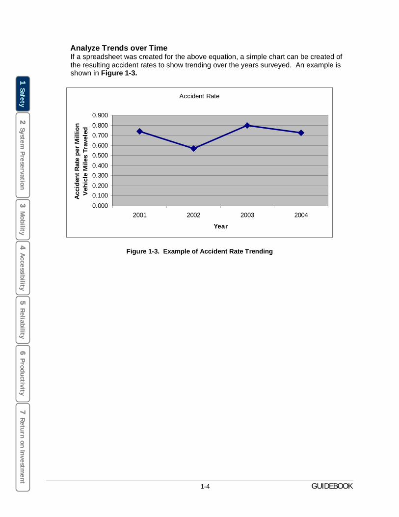
� Analyze Trends over Time If a spreadsheet was created for the above equation, a simple chart can be created of the resulting accident rates to show trending over the years surveyed. An example is shown in Figure 1-3.

Accident Rate

0.000 0.100 0.200 0.300 0.400 0.500 0.600 0.700 0.800 0.900

2001 2002 2003 2004

Year

Acci

dent

Rat

e pe

r M

illio

nVe

hicl

e M

iles

Trav

eled

Figure 1-3. Example of Accident Rate Trending

1-4 GUIDEBOOK

Quick Reference

Safety Performance Measure

§ Accident rate per million vehicle miles traveled

InputsData needed

Necessary As Feasible Accident Data for current year from: § County Data § CHP § SWITRS

Length of Roadway (miles)

AADT for current year (can obtain from Caltrans website for state routes)

Accident Data for as many previous years as available § County Data § CHP § SWITRS

AADT for previous years (can obtain from Caltrans website for state routes)

OutputsResults

calculated

Accident rate per million vehicle miles traveled.

Trend analysis for accident rate if more than one years’ data is available.

1-5 GUIDEBOOK

1 Safety

2 System

Preservation 3

Mobility

4 A

ccessibility 5

Reliability 6

Productivity7


Section 2 System Preservation


System Preservation refers to maintaining the condition of the roadway network at a desired or agreed upon level. Preservation of the roadway network is a critical priority for most rural counties given that maintained roadways allow for ease of travel for the public and their vehicles, both within and between counties. Simply performing routine maintenance is challenging given fiscal realities in rural areas and is rarely sufficient to insure adequate system preservation. In order to accurately and consistently document system preservation needs, rural agencies should keep records of all current conditions and all maintenance work to thoroughly document roadway conditions and to assist with forecasting resource needs, including funding, for vital future maintenance, rehabilitation, and reconstruction projects. Caltrans maintains the Highway Performance Monitoring System (HPMS) database for the State Highway System, and provides access to this data for each county. However, the data associated with local roads within the county are left up to individual jurisdictions.

Pavement management systems (PMS) are the primary tools for measuring and reporting roadway conditions. Additionally, a properly maintained and updated PMS can be used to forecast pavement deterioration over time, calculate costs for various improvement projects, and identify maintenance strategies based on different investment and funding scenarios.

2-1 GUIDEBOOK

3 M

obility 4

Accessibility

5 Reliability

6 Productivity

2 System

Preservation 7


1 Safety

How Would a Rural Area Measure System Preservation?

Counties vary in the amount of effort and budget that they can devote to the collection of pavement data; often there are not appropriate resources to maintain an adequate PMS. The step-by-step guidance that follows is presented for each of the three experience levels.

If a rural area: System Preservationmeasurement could be considered:

System Preservationwould be measured using:

§ Has no pavement monitoring

Basic § Formal pavement inspections

§ Manages pavement § Spreadsheet-based database in Excel or pavement inventory other spreadsheet § Record of current and program future maintenance

§ Performs reactive needs maintenance based on citizen requests

§ Maintains a formal Intermediate § A fully updated PMS PMS § A PMS to generate

§ Generates PCI reports reports to assess § Records maintenance pavement condition

information and allocate resources § No forecasting § Maintenance records in

PMS for use with funding scenarios to plan for future needs

§ Has the characteristics of Intermediate programs

§ Forecasts future deterioration and maintenance

§ Utilizes funding forecasts to allocate resources

Advanced § A fully updated PMS and a GIS linking it with PMS information

2-2 GUIDEBOOK

3 M

obility 4

Accessibility

5 Reliability

6 Productivity

2 System

Preservation 7


1 Safety

1.


At the Basic level a county is assumed to be just beginning a pavement management database. It is assumed that field inspections have not been performed, and that a PMS is not typically being used. If the county has purchased a PMS, they can use the guidance provided in this section to learn how to populate the database, though the exact techniques might vary based on the type of program purchased. Counties in this category would likely have their own method of keeping a database, typically in a spreadsheet program like Excel.

� Become Familiar with Pavement Distress Types A Pavement Condition Index (PCI) is generally based on a survey of the seven different distress types listed below. There are additional distress types that may be identified, but these seven are the most typical to examine. Distress surveys are designed to answer three questions: what is wrong (distress type), how bad is it (severity), and how much distress is present (density)? The seven distress types are shown in the box below.

Distress Types

1. Alligator Cracking 2. Block Cracking 3. Distortions 4. Longitudinal and Transverse (LT) Cracking 5. Patching and Utility Cut Patching 6. Rutting and Depressions 7. Weathering and Raveling

The distress types, characteristics, and measurement techniques are summarized in the Technical Supplement, System Preservation Section.

� Conduct Pavement Inspections The methods for the physical inspection of the roadway outlined below can be utilized for input into a formal PMS program, or for a less advanced spreadsheet-based system.

Inspections are typically performed for about 10% of a roadway, or 100 feet for every 1000 feet of road surface. Inspections are performed on “representative samples” of a road, which is to say that the segments inspected should encompass the overall condition of the roadway, and represent neither the best nor the worst conditions of the road as a whole. The inspections should be done for every roadway in a jurisdiction, be it by city or by county. This could be done all in the same year, or on a rotating basis, meaning that a portion of a jurisdiction would be surveyed each year, and thus the total mileage would be surveyed every X number of years as outlined in a pavement management plan. Where a lack of funding renders a jurisdiction unable to perform this process fully, it is encouraged that at least the major, most heavily traveled (traffic volume and/or heavy vehicle volume) local roads be surveyed, or that a lesser percentage of each roadway be inspected. Additionally, counties are encouraged to take advantage of Caltrans’ HPMS resource, which contains road conditions of the State Highway System (SHS) for each county.

2-3 GUIDEBOOK

3 M

obility 4

Accessibility

5 Reliability

6 Productivity

2 System

Preservation 7


1 Safety

3 M

obility 4

Accessibility

5 Reliability

6 Productivity

2 System

Preservation 7


1 Safety

If using a PMS, individual reports for each street segment can be generated and printed out for use during field inventories. The paper forms are filled out in the field and the data is entered into a computer at a later time. Another method that some PMS programs may support is a database stored in a handheld Personal Digital Assistant (PDA) that allows field inspection data to be input into the PDA then uploaded at the end of the day to an office PC and main database. If using a spreadsheet program like Excel, a blank form could be created for each street segment showing the seven distresses and severity levels, which could be taken into the field and filled out.

In the field, verify street width. Then, using a measuring wheel and pavement spray paint, mark off a 100-foot length of roadway. However, if the width is greater than 40 feet, only a 50-foot section should be surveyed for every 1,000 feet of roadway. The width of the roadway will help in determining the square footage of the section: if the street is 26-feet wide, the segment will be 2,600 square feet (26 x 100 = 2,600). The distress type determined for the sample is then applied to the entire 1,000-foot street length, which is why selection of a ”representative sample” is key.

Next is the measurement of each distress type. Several different levels of severity may exist within the same area, so carefully separate them to accurately measure and record the information. These measurements are most easily made with a measuring wheel.

� Compile Data If using a PMS, transfer the data from the field inspection forms into the computer database.

If just beginning, use a spreadsheet to track densities of the distresses over time as an introduction to the use of the pavement management software. This information will then be easy to enter into a PMS when the county acquires it. For an Excel database, create a spreadsheet showing the street segment name, limits, width, length of segment (typically 100 ft.), the seven major distresses, and the three severity levels for each. Then enter the field data under the appropriate columns.

Create a new column that calculates the square footage of the segment (width x length). Then, create a column that will sum the total measurements done in the field (all distresses and all severity levels). Though some distresses are in linear feet, we will assume that they have a width of one foot for this calculation. Next, create a column that divides the sum of distresses by the total square footage of the segment. Format the column so that it is a percentage. This will be the percentage of the segment by distress type. This scale is a high level and general measurement of the pavement condition, and is not meant to be compared used for comparing counties or in place of the traditional PCI rating scale. It is purely meant to give a county a means by which to begin measuring pavement condition, and to have a starting point on which to build its pavement management program. This scale is also more linear than the typical pavement condition scales, and counties are encouraged to use this as a guide.

0-30% Good 31-60% Fair

61-100% Poor

This scale would indicate that if a roadway surface is 0-30% distressed, it is in ‘Good’ condition, and does not require immediate maintenance. A roadway with 31-60% of the surface distressed would be in ‘Fair’ condition, and would require more immediate

2-4 GUIDEBOOK

attention such as a slurry seal, crack seals, or other preventative maintenance and/or repair. A roadway that receives a rating of ‘Poor’, or 61-100% distressed, would require immediate attention such as reconstruction or repaving as soon as the budget allows.

Manual calculations of PCI are possible, but very time consuming due to the necessity to look up information on detailed graphs for each distress by severity level to determine the corresponding value to deduct from the overall PCI to reflect the impact of that amount of distress. These values are called ‘deduct values’ and are calculated automatically by PMS software. When the need for PCI calculations and information arises, the county should consider investing in a PMS program.

� Log Maintenance Data On a separate Excel tab, a maintenance log file should be created to keep track of the maintenance work done and/or scheduled on the roadway segments. This information can be used to predict future maintenance needs. For example, if the date of a road rehabilitation is entered, a reasonable estimation can be made as to when chip seals, slurry seals, etc. will be required based on available historical data . This can also be used for a preliminary start to a PCI database given that pavement that is new has a PCI of 100, and deteriorates along a known curve.

� Consider Pavement Management Programs After beginning to build a pavement condition database, the county should consider making the investment in a PMS. These programs are the preferred method for maintaining a database of pavement conditions and maintenance and rehabilitation (M&R) information. They are also used as tools to predict M&R needs many years into the future based on different funding scenarios. The two main pavement management systems used in California are StreetSaver and MicroPAVER.

StreetSaver was developed by the Bay Area Metropolitan Transportation Commission (MTC) as a three-part solution to the issue of local jurisdictions not performing timely pavement maintenance and upkeep. The program’s aim was to provide a pavement condition index (PCI) for maintenance treatments in the Bay Area, and a network level assignment procedure. Two versions of StreetSaver are available for use: a web-based interface and a desktop program. Both versions are available to customers outside of the Bay Area for a slightly higher cost. The online version has a yearly subscription fee, while the desktop version has a one-time fee. Training and tutorials are available through the MTC. StreetSaver allows for field data collection via printed paper forms or handheld PDAs. Analysis available through StreetSaver includes budget needs for maintenance, impacts of various funding situations, event-based calculation, and project selection. Reports that can be generated include 30 standard reports and graphs, customized reports, depreciation method, Geographic Information System (GIS) linkage, and reports fitting the requirements of Government Accounting Standards Board Statement 34 (GASB 34), which requires local governments to begin reporting the value of their infrastructure assets, including roads, bridges, water and sewer facilities and dams, in their annual financial reports on an accrual accounting basis.

MicroPAVER was first developed by the Army Corps of Engineers to help manage maintenance and rehabilitation of the Department of Defense’s pavement inventory. It uses the PCI index to describe the current pavement condition and to predict future M&R needs, and provides an analysis of where to allocate maintenance funding. Field data may be entered into MicroPAVER from either paper forms or handheld devices. The

2-5 GUIDEBOOK

3 M

obility 4

Accessibility

5 Reliability

6 Productivity

2 System

Preservation 7


1 Safety

reports section of MicroPAVER offers numerous options to provide basic pavement information: summary charts, standard reports (branch listing, work history, etc.), re-inspection reports, user-defined reports (ability to create custom reports), and GIS reports (preset views that show information in a graphical display; available when a map has been linked to the database). Forecasting abilities of MicroPAVER include prediction modeling and work planning (including budget consequences, elimination of M&R backlog calculations, steps toward reaching preferred PCI, etc.). MicroPAVER training is available through the University of Illinois, Urbana-Champaign.

Step-By-Step Guidance Intermediate

It is assumed that a county with Intermediate system preservation capabilities has a PMS installed and populated, and that its users are well-versed in the seven major distress types and field inspection techniques. For more information on these, see the Technical Supplement, System Preservation Section.

� Conduct Field Inspections At this level, field inspections should be performed on at least 5% of the roadway, if not the full 10%. Additionally, the county should aim for completing inspections of all local roadways, not only the most traveled corridors. This could be done all at once, or divided into a rotating cycle (for example, one third of the roadways would be inspected each year, so there is a full set of data every three years). Caltrans data for the State Highway System can be obtained from the HPMS system and integrated with local data.

� Compile Reports After inspections, data should be entered into the database. Other necessary information such as maintenance and rehabilitation data should be entered as the tasks are completed, or at a specified time in the inspection cycle. After the database is populated, reports can be generated. The sample report presented below is the basic report that provides a snapshot of current system conditions.

� PCI Calculation Figure 2-1 on the following page was created using StreetSaver; other programs generate roughly the same information.

1 Safety

2 System

Preservation 3

Mobility

4 A

ccessibility 5

Reliability 6

Productivity7


2-6 GUIDEBOOK

• PCI Date: The date on which the PCI was calculated • Old PCI: The most recent data prior to this report • PCI: The new PCI for the segment • Pct Load: The percent of distress caused by loading factors • Pct Envr: The percent of distress caused by environmental reasons • Pct Other: The percent of distress caused by other factors

Figure 2-1. PCI Calculation Summary Report (Source: MTC StreetSaver)

The information presented above includes the Street ID, Section ID, Street Name, Beginning/Ending location, Inspection Date, Previous PCI, New PCI, and other calculations. This is the master database of all PCI calculations for the county.

This information can also be presented as a graph to show the weighted average PCI for the county.

1 Safety

2 System

Preservation 3

Mobility

4 A

ccessibility 5

Reliability 6

Productivity7

Return on Investment2-7 GUIDEBOOK

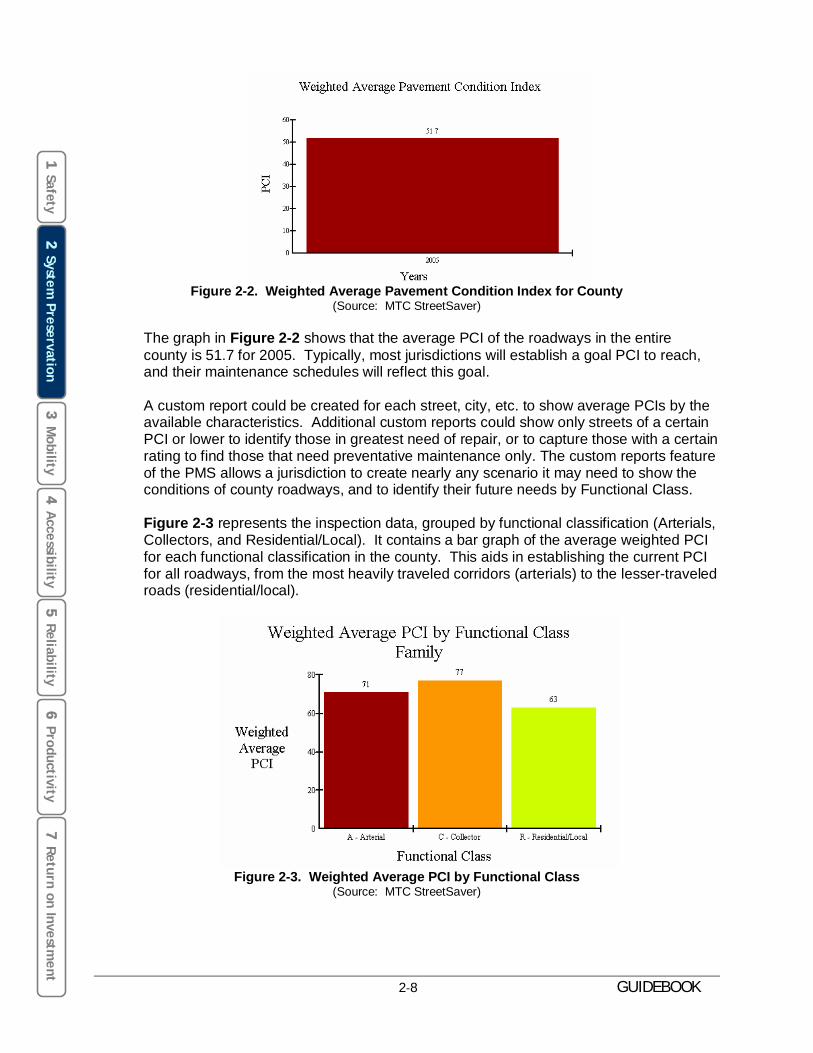
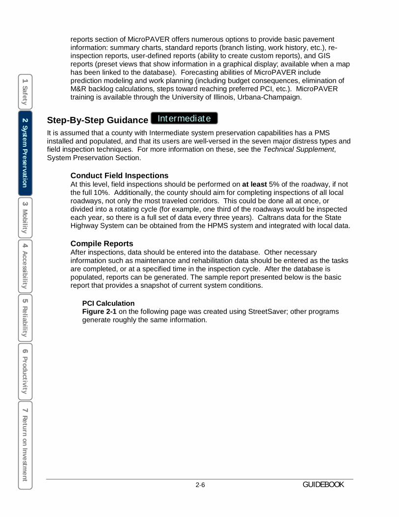
Figure 2-2. Weighted Average Pavement Condition Index for County (Source: MTC StreetSaver)

The graph in Figure 2-2 shows that the average PCI of the roadways in the entire county is 51.7 for 2005. Typically, most jurisdictions will establish a goal PCI to reach, and their maintenance schedules will reflect this goal.

A custom report could be created for each street, city, etc. to show average PCIs by the available characteristics. Additional custom reports could show only streets of a certain PCI or lower to identify those in greatest need of repair, or to capture those with a certain rating to find those that need preventative maintenance only. The custom reports feature of the PMS allows a jurisdiction to create nearly any scenario it may need to show the conditions of county roadways, and to identify their future needs by Functional Class.

Figure 2-3 represents the inspection data, grouped by functional classification (Arterials, Collectors, and Residential/Local). It contains a bar graph of the average weighted PCI for each functional classification in the county. This aids in establishing the current PCI for all roadways, from the most heavily traveled corridors (arterials) to the lesser-traveled roads (residential/local).

Figure 2-3. Weighted Average PCI by Functional Class (Source: MTC StreetSaver)

1 Safety

2 System

Preservation 3

Mobility

4 A

ccessibility 5

Reliability 6

Productivity7


2-8 GUIDEBOOK

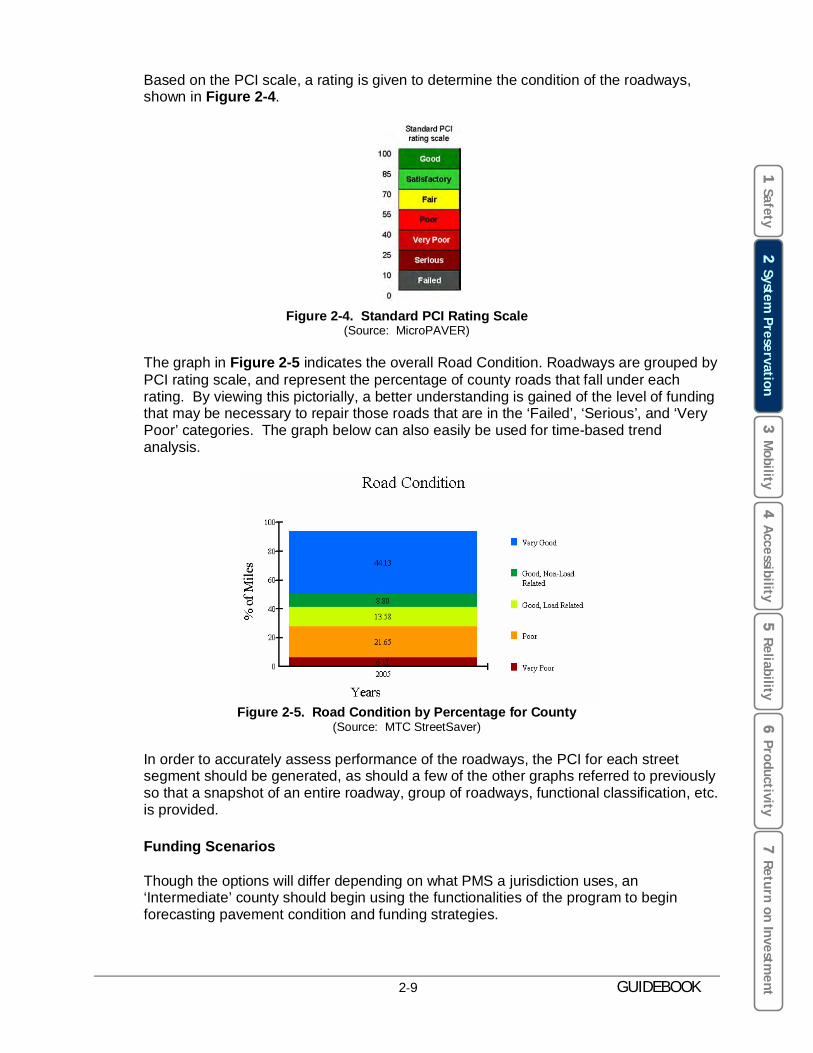
Based on the PCI scale, a rating is given to determine the condition of the roadways, shown in Figure 2-4.

Figure 2-4. Standard PCI Rating Scale(Source: MicroPAVER)

The graph in Figure 2-5 indicates the overall Road Condition. Roadways are grouped by PCI rating scale, and represent the percentage of county roads that fall under each rating. By viewing this pictorially, a better understanding is gained of the level of funding that may be necessary to repair those roads that are in the ‘Failed’, ‘Serious’, and ‘Very Poor’categories. The graph below can also easily be used for time-based trend analysis.

Figure 2-5. Road Condition by Percentage for County (Source: MTC StreetSaver)

In order to accurately assess performance of the roadways, the PCI for each street segment should be generated, as should a few of the other graphs referred to previously so that a snapshot of an entire roadway, group of roadways, functional classification, etc. is provided.

� Funding Scenarios

Though the options will differ depending on what PMS a jurisdiction uses, an ‘Intermediate’ county should begin using the functionalities of the program to begin forecasting pavement condition and funding strategies.

1 Safety

2 System

Preservation 3

Mobility

4 A

ccessibility 5

Reliability 6

Productivity7


For example, the screenshot in Figure 2-6 shows the starting point for budget scenarios in StreetSaver:

Figure 2-6. Screenshot of Budget Scenarios Worksheet (Source: MTC StreetSaver)

The following definitions apply to Figure 2-6:

Interest Interest rate used during Scenario Inflation Inflation rate used during Scenario Budget Base budget for Scenario PM % Preventative maintenance percent

for Scenario

Based on the values entered for the interest rate, inflation rate, and budget, projected PCI for the county and individual segments can be determined, as can a cost summary for projected necessary maintenance in future years.

1 Safety

2 System

Preservation 3

Mobility

4 A

ccessibility 5

Reliability 6

Productivity7


2-10 GUIDEBOOK

Figure 2-7. Projected PCI’s and Future Needs (Source: MTC StreetSaver)

The report in Figure 2-7 lists the potential future year PCI for each street segment if left untreated, as well as the future year PCI if preventative maintenance is performed. This information can be utilized to plan funding strategies for future maintenance and to properly gauge the funding necessary to keep the roadways at a desired or agreed upon level. Information can also be generated as to the funding necessary to bring the overall PCI of the county up to a goal level by a certain date. Generating such information is required in order to accurately link future roadway performance with future budget needs.

� Log Maintenance Data

Once the database is populated, maintenance information should be entered into the program. This can be done on an ongoing basis, as work is completed and/or scheduled.

Most PMS programs allow users the ability to add maintenance treatments, costs, and other information to the program. This information can then be used to generate reports based on available funding, as explained above. Data is stored in a computer to allow sorting based on different scenarios and criteria. The screenshot in Figure 2-8 on the following page shows the StreetSaver Table Maintenance window where historical treatment descriptions are available. The tabs denote different aspects of maintenance that can be viewed. The data assists in not only providing an historical context for the condition of the roadways, but also in providing cost information that serves as input into budget estimates that are used in forecasting scenarios.

1 Safety

2 System

Preservation 3

Mobility

4 A

ccessibility 5

Reliability 6

Productivity7


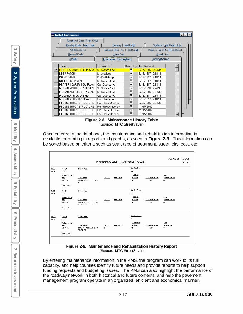
Figure 2-8. Maintenance History Table (Source: MTC StreetSaver)

Once entered in the database, the maintenance and rehabilitation information is available for printing in reports and graphs, as seen in Figure 2-9. This information can be sorted based on criteria such as year, type of treatment, street, city, cost, etc.

Figure 2-9. Maintenance and Rehabilitation History Report (Source: MTC StreetSaver)

By entering maintenance information in the PMS, the program can work to its full capacity, and help counties identify future needs and provide reports to help support funding requests and budgeting issues. The PMS can also highlight the performance of the roadway network in both historical and future contexts, and help the pavement management program operate in an organized, efficient and economical manner.

1 Safety

2 System

Preservation 3

Mobility

4 A

ccessibility 5

Reliability 6

Productivity7


2-12 GUIDEBOOK

Step-By-Step Guidance Advanced

It is assumed that an advanced-level county currently uses a PMS program to manage pavement inventory. It is also assumed that the county is using the program to forecast future pavement conditions and maintenance needs, and is taking advantage of the program’s budgeting capabilities to help make fiscal decisions.

� Populate Database A county classified as advanced is anticipated to have a full set of data populating the PMS database for at least one full inspection cycle, and be well versed in the process of completing a county-wide pavement inspection. At this point, it is recommended that the county aim to complete this cycle once per year, so that the data is up to date so as to forecast maintenance and deterioration as completely and accurately as possible. This full inspection should by now include all roadways that are not state-owned.

The maintenance information should also be updated to accurately reflect current work being done on the roadways, and to keep the prices of supplies, materials, and labor current. Financial analysis done through the PMS should be more sophisticated for these counties, including 10-15 year maintenance needs, various maintenance strategies based on different funding scenarios, and maintenance and rehabilitation with PCI goals in mind.

� Consider GIS Linkage One additional aspect of the PMS that advanced-level counties may consider taking advantage of is linking the pavement condition database with maps using a Geographic Information System (GIS). Such linkage allows a color-coded visual presentation of the PCI of various areas of the county on a map. While using a color-coded map it is possible to identify trends based on geographical area, and to determine if traffic volumes, congestion, or population densities would impact decisions on maintenance schedules and funding.

Figure 2-10. Screenshot of How to Export Data to GIS Program (Source: MTC StreetSaver)

1 Safety

2 System

Preservation 3

Mobility

4 A

ccessibility 5

Reliability 6

Productivity7


Though the process will vary from program to program, one method to link a pavement inspection database to a GIS is to use the ‘Export Data’ function in the PMS as shown on the previous page in Figure 2-10. The user elects to export GIS data, and then selects the type of data to be exported (typically at least the pavement condition information). This function, in other programs, may only be available once a map is linked to the database. It is possible that an additional program may be required for this function. Linkage to a GIS program is not necessary to calculate performance measures, but it is an additional tool that can provide a geographical view of overall pavement condition to further enhance knowledge of the performance of the roadway system and presentation of enhanced knowledge to customers and decision-makers. When completed, the GIS pavement management map will look similar to the image in Figure 2-11.

The PCI score is shown in ranges, with a score falling between 81-100 indicating the best maintained roadways

Figure 2-11. Example of GIS Linkage (Source: Sonoma County, Farallon Geographics)

The map above incorporates the PCI information collected through the pavement management system for the county with a GIS map of the roadways. In the legend on the right, there are many options for layers to turn on within the map to show certain attributes. In the specific area shown above, the PCI for those roadways is shown, and correlates to the colors in the legend. The PCI score is shown in ranges, with 81-100 indicating the best maintained roadways.

1 Safety

2 System

Preservation 3

Mobility

4 A

ccessibility 5

Reliability 6

Productivity7


2-14 GUIDEBOOK

Quick Reference

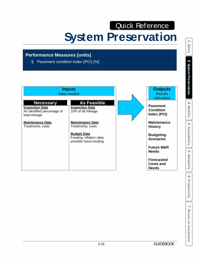
System Preservation Performance Measures [units]

§ Pavement condition index (PCI) [%]

InputsData needed

Necessary As Feasible Inspection Data An identified percentage of total mileage

Maintenance Data Treatments, costs

Inspection Data 10% of all mileage

Maintenance Data Treatments, costs

Budget Data Funding, inflation rates, possible future funding

OutputsResults

calculated

Pavement Condition Index (PCI)

Maintenance History

Budgeting Scenarios

Future M&R Needs

Forecasted Costs and Needs

1 Safety

2 System

Preservation 3

Mobility

4 A

ccessibility 5

Reliability 6

Productivity7


2-15 GUIDEBOOK

Section3 Mobility


Mobility refers to the ease or difficulty of traveling from an origin to a destination. Mobility refers to the potential for movement, or the ability to travel from point A to point B. Mobility implies both a means (vehicle) and a way (route, path, or line) and is closely linked to accessibility which is addressed in the next section of this guidebook. As mobility increases, accessibility tends to improve; therefore, more destinations can be reached or more means and ways are available to reach desired destinations. As mobility decreases, accessibility tends to become increasingly restricted; therefore, travel becomes more difficult and limited depending on cost considerations. A rural area may have high mobility due to low traffic volumes, but it may have low access potential due to greater distances between origins and destinations.

Rural areas have typically used Level of Service (LOS) to assess how roadways or intersections along roadways help or impede movement. LOS includes six broad categories (A-F) that are used to estimate roadway operations. LOS does not always allow for trend analysis or for evaluating the effectiveness of smaller congestion relief investments that might ease congestion without changing the LOS. Thus, in order to quantify mobility, the following information is needed: § Travel time between specific points along major corridors. § Speed. § Delay. Although the causes of delay in rural and urban areas may differ (for example,

increased potential for landslides in rural areas, or extreme delays due to incidents affecting high volumes of traffic in urban areas), delay is measured in the same way for both areas regardless of the cause.

Depending on the availability of automated detection and travel demand model output, different combinations of performance measures might be calculable. Furthermore, output from automated detection stations can be transmitted to

free the Caltrans Freeway Performance Measurement System (PeMS), a free web-resource based cooperative project through which freeway performance measures are

calculated, including those recommended above. The PeMS output will properly reflect traffic conditions in rural areas if traffic data from detection stations in those rural areas is directly provided.

3-1 GUIDEBOOK

1 Safety

3 M

obility 2

System Preservation

4 A

ccessibility 5

Reliability 6

Productivity7


How Would a Rural Area Measure Mobility?

The most effective methodology depends on factors such as data availability, resources, and expertise. As resources increase or expertise improves, so will the ability to quantify mobility at an increasingly accurate level, where ‘increased accuracy’ might result in greater detail, greater geographical coverage, or increased sample size over different days depending on local needs. The table below outlines possible performance measures corresponding to different levels of data availability.

If a rural area: Mobility measurement capabilities could be considered:

Mobility would be measured using:

§ Has not measured mobility

§ Uses probe vehicles

Basic § Travel times

§ Has automated Intermediate TDM output: detection § Travel times

§ Uses a Travel Demand § Speeds Model (TDM) § Delay

If TDM is unavailable, can transmit the data to PeMS

§ Has extensive Advanced TDM output: automated detection § Travel times

§ Uses a TDM § Speeds § Transmits data to § Delay

PeMS If TDM is unavailable, can transmit the data to PeMS

For urban and urbanizing areas periods of high traffic demand typically occur during weekday AM and PM peak periods, but in rural areas that experience high recreational demand, peak periods typically occur on weekends.

1 Safety

3 M

obility 2

System Preservation

4 A

ccessibility 5

Reliability 6

Productivity7


3-2 GUIDEBOOK


� Choose Coverage and Time Depending on a rural area’s intended purpose for calculating mobility performance measures, a rural area might find it more useful to select either specific corridors, or a number of corridors that can be analyzed for a specific time or over-time using trend analysis. Trend analysis can be conducted over several months under changing development conditions, year by year to reflect area growth and development, or for other time periods depending on local needs. Whatever time frame is selected, it should be specifically laid out in the initial scope of work. Once the scope is specified, a rural area should consider repeating the exact same data collection and calculation procedures at regular intervals in the future (possibly every year, every two years or whatever best suits needs and resource availability). As with other traffic data collection, data should be collected during typical weekday peak periods between Labor Day in September and Memorial Day in May (For urban and urbanizing areas peak periods are typically 6AM-9AM and 4PM-6PM, but this varies by location. For rural areas that experience high recreational demand, peak periods typically occur on weekends.)

� Identify Endpoints Endpoints of the major corridors, or congested segments within corridors, selected within the rural area in Step � should be identified. These endpoints are also called origin-destination (OD) pairs. Endpoints should be easily visible and detailed sufficiently so that any number of people (if manual data collection is performed with probe vehicles) performing the procedure are able record repeat observations consistently, at exactly the same location. § For example: “For the eastbound Lake Avenue segment,

o Point A = near side of Grove Street intersection o Point B = near side of on-ramp to Highway 9”

� Record Posted Speeds Record posted speed limits along the previously identified corridors or segments wherever they differ from those of an adjacent segment.

� Perform Probe Vehicle Run(s) Perform probe vehicle runs along the corridors or segments identified previously. Probe vehicle data collection may be manual or automated (electronic measuring devices or Global Positioning System (GPS) attached to vehicles). Field staff can collect either travel times or speeds between Point A and Point B on the selected route(s) or segment(s), and calculate the other measures from those results. Travel times are usually the easiest data to collect. § Manual probe vehicle data collection. If collecting data manually, the driver of

the probe vehicle should record travel times from Point A to Point B along with the time of day, and observations about unusual traffic conditions (such as incidents) that might affect the results. As feasible, repetitions should be performed for the same route (at least two to provide a sample from which to average). Speeds can also be collected using this technique.

§ Measuring devices or GPS used with probe vehicles. A rural agency may consider investing in speed measuring instrumentation or a GPS for probe vehicles. Such instrumentation makes field data collection faster and safer, and provides more accurate data. Data can also be used for other performance measures, such as

3-3 GUIDEBOOK

3 M

obility 4

Accessibility

5 Reliability

6 Productivity

2 System

Preservation 7


1 Safety

3 M

obility 4

Accessibility

5 Reliability

6 Productivity

2 System

Preservation 7


1 Safety

reliability. Speed measuring instrumentation would attach to the probe vehicle and record odometer readings automatically during the driver’s trip. GPS instrumentation usually consists of an antenna and small GPS device with a user interface, which records vehicle position automatically in terms of standard map coordinates (latitude and longitude). Software usually accompanies such speed measuring instrumentation or GPS instrumentation and allows extraction of the desired measures (travel times or speeds, or possibly even delays) based on the raw recorded observations. In some cases, post-processing may be required (using simple spreadsheet functions) in order to manipulate the raw data to calculate the desired measures.

� Ensure that Analysis is Performed for Individual OD Pairs and Not In Aggregate for the Entire Rural Area Aggregation of data for multiple corridors or for an entire rural area (such as a county) is not advised. The performance measures calculated using the techniques described above are best used for analysis of individual OD pairs.

� Calculate Performance Measures Once travel times or speeds have been collected using a probe vehicle (and the device output processed, if necessary), the suggested measures can be calculated as follows:

Travel time, if not collected directly, is calculated by dividing the distance between the origin and destination by the average speed:

Travel Time (in hours) = Distance (in miles) /Average Speed (in miles per hour)

Delay is calculated by subtracting travel time under ideal conditions (for example, posted speeds) from actual travel times measured while driving each segment(s):

Actual Travel Time (in hours) = Distance (in miles) /Actual Average Speed (in miles per hour)

Optimal Travel Time (in hours) = Distance (in miles)/Posted Speed (in miles per hour)

Delay (in hours) = Actual Travel Time (in hours) – Optimal Travel Time (in hours)

� Analyze Trends over Time A spreadsheet can be used to track results over regular time intervals (for example, every year) to quantify how conditions have improved or worsened over time for the corridor(s) or segment(s) selected.

3-4 GUIDEBOOK


This Intermediate category applies to rural areas which have automated detection (detection which is assumed to cover the major corridors or segments of interest). The rural areas should also have access to a regional or local Travel Demand Model (TDM).

� Identify Study Area and Endpoints Endpoints of the major corridors, or congested segments within corridors, should be identified. These endpoints are also called origin-destination (OD) pairs.

� Identify and Collect the Required Data from Detection Stations With automated detection, a large amount of data can be collected and analyzed. The data should consist of speed data which will allow measures such as travel times and delays to be calculated. As described above, this Intermediate guidance assumes that detection stations are located along all corridors or segments of interest between the OD pairs identified in Step �. It is useful to be able to analyze one year’s worth of peak period data for the selected corridor(s) or segment(s). If one year’s worth of data has not been archived or is unavailable, data should be collected for as much time as possible.

� Enter Data into the Travel Demand Model (TDM) It is recognized that TDM resources may not be in-house, and that coordination with the agency who maintains and runs the TDM may be necessary. Working with the TDM-owning agency if and where appropriate, data collected in Step � should be prepared according to the TDM-specific requirements, and input into the TDM.

� Obtain Output from the TDM Obtain output from the TDM of the requested measures of travel time, speed, and delay between the selected OD pairs.

� Ensure that Analysis is Performed for Individual OD Pairs and Not in Aggregate for the Entire Rural Area Aggregation of data for multiple corridors or for an entire rural area (such as a county) is not advised. The performance measures calculated using the techniques described above are best used for analysis of individual OD pairs.

� Analyze Trends over Time A simple spreadsheet can be used to track results over regular time intervals (for example, every year) to quantify how conditions have improved or worsened over time for the selected corridor(s) or segment(s).

3-5 GUIDEBOOK

3 M

obility 4

Accessibility

5 Reliability

6 Productivity

2 System

Preservation 7


1 Safety


To facilitate repeated analysis of corridors outfitted with automated detection, the use of PeMS should be considered. PeMS is the acronym for the Freeway Performance Measurement System Project. The Project, a joint effort by

free Caltrans, the University of California, Berkeley, and the Partnership for Advanced resource Technology on the Highways (PATH) involves the investigation of various freeway system performance measures. The software developed in conjunction with the PeMS project, is a web-based traffic data collection, processing and analysis tool used to assist in assessing the performance of the freeway system. PeMS extracts information from real-time and historical data and presents it in various forms to assist managers, traffic engineers, planners, freeway users, researchers, and traveler information service providers (value added resellers or VARs) with a variety of data and informational needs. The address of the PeMS website is http://pems.eecs.berkeley.edu/Public/.

PeMS can be used to provide output such as travel times and other measures directly, using a feed from an automated detector located on any roadway (whether State or Local). If PeMS is to be used to process output, the procedure below to connect automated detectors to PeMS should be followed.

� Contact PeMS Staff Regarding Connection of Rural Detectors to PeMS Contact information can be found at the PeMS website: http://pems.eecs.berkeley.edu/Public/. Staff can provide additional details and documentation regarding the integration requirements listed below.

� Gather Information About the Local Detector System Although agency representatives are guided through the integration process, PeMS staff requires information such as the following to begin: § Traffic data types collected - flow, occupancy, speed § Geospatial data - list of roadways, orientation (N., S., E., W.), and designation (State

road, arterial, etc.); and if desired, geographic regions (for example, a list of towns within the rural area if town name is an attribute); or postmiles or odometer readings from stations identified by latitude and longitude

§ Equipment configuration - complete identification of field elements such as controllers, stations, and detectors. Required and optional attributes can be explained by the PeMS staff

§ Configuration management - how to ensure that any changes to the above information will be communicated to PeMS

§ Data feeds - this is documentation about the data itself and can usually be provided by automated detector vendors

� Electronically Transmit Rural Area Detector Data to PeMS After the PeMS staff assists the rural area with connections and data compatibility issues, the rural area can then transmit detector data to PeMS directly.

1 Safety

3 M

obility 2

System Preservation

4 A

ccessibility 5

Reliability 6

Productivity7


3-6 GUIDEBOOK

http://pems.eecs.berkeley.edu/Public/.


� Apply for a Free PeMS Account Anyone is eligible to obtain a user account. Once logged in to a PeMS account online, the user can retrieve and manipulate the data of interest. All that is requested to obtain an account is name, phone, email address, agency name, and reason for use.

� Select Study Parameters Before logging into PeMS, study parameters such as roadways, roadway segments, times of day, and date range of interest should be chosen.

� Login and Obtain Outputs from PeMS Once logged into PeMS, users may select a roadway segment of interest, and output travel times. Users may select date ranges, exclude certain days, and specify granularity (hours, days, etc.). In addition, the output can be viewed as a plot or table, and can be exported as text or an Excel file. An example of travel time output for a corridor is shown in Figure 3-1.

Figure 3-1. PeMS output and capabilities (Analyzing roadway segment in Santa Cruz)

1 Safety

3 M

obility 2

System Preservation

4 A

ccessibility 5

Reliability 6

Productivity7


3-7 GUIDEBOOK

3 M

obility 4

Accessibility

5 Reliability

6 Productivity

2 System

Preservation 7


1 Safety


� Analyze Trends over Time Once data is exported from PeMS into Excel, the data can be used to track results over regular time intervals (for example, every year) to quantify how conditions have improved or worsened over time for the selected corridor(s) or segment(s).

3-8 GUIDEBOOK

Quick Reference

Mobility Performance Measures [units]

§ Origin-destination travel times along major corridors [min] § Actual Average Speeds [mph] § Delays [sec or min]

InputsData Needed

Necessary As Feasible Speeds between major origin-destination pairs from any of: § probe vehicles with speed

measuring devices and/or GPS, or

§ automated detection, or § Travel demand model

(TDM) output

OR

Travel times between major origin-destination pairs from any of: § probe vehicles with speed

measuring devices and/or GPS, or

§ automated detection, or § TDM output

Distances between the selected origin and destination points (if a route passes through areas with different posted speeds, the route should be broken into segments for the analysis)

Posted speed limit(s) between origin and destination points

If available, Travel times between major origin-destination pairs as output directly from TDM

If available, delays as output directly from TDM

If automated detection is being used, consider sending the input data to the California Freeway Performance Measurement System (PeMS) which will then process the data and provide the mobility measures recommended

free resource

OutputsResults

Calculated

Trend analysis over time of:

§ Travel times § Speeds § Delays

The longer the time period for which data is collected and analyzed, the more informative the result.

If data is sent to PeMS for processing, the recommended mobility measures (travel times, speeds, delays) will be provided.

1 Safety

3 M

obility 2

System Preservation

4 A

ccessibility 5

Reliability 6

Productivity7


3-9 GUIDEBOOK

Section 4 Accessibility


Accessibility is defined as the opportunity and ease of reaching desired destinations. The fundamental product and intended purpose of a transportation system is to provide the opportunity for people and goods to physically reach or access desired destinations. The overall accessibility of a given geographic area may be increased in many ways, but the two main ways are either to provide a greater supply of transportation (for example an increase in lane miles of roadway or mass transit service frequencies), or to increase the options for travel (usually in terms of the availability of different transportation modes).

Accessibility is especially important in rural areas where the State Highway System (SHS) is the only option for interregional travel. In such areas, not only is interregional accessibility important, but also of particular concern is accessibility to the SHS using the local road system as secondary or optional routes for accessing the SHS may be either unavailable or time prohibitive. In other words, if the primary route for accessing the SHS is blocked, a comparable alternative is not only desirable, but in emergencies, critical.

How Would a Rural Area Measure Accessibility?

Depending on available resources, there are three experience levels listed on the following page that indicate the guidance to follow for developing the accessibility measure.

4-1 GUIDEBOOK

3 M

obility 4

Accessibility 5

Reliability 6

Productivity2

System Preservation

7 Return on Investm

ent1

Safety

If a rural area: Accessibility measurement capabilities could be considered:

Accessibility would be measured using:

§ Is using hard copy maps

§ Only wishes to calculate accessibility for selected points of interest or selected roadways of interest

Basic § Manual calculations

§ Has commercial mapping software

§ Wishes to refine measurements with population data

§ Wishes to calculate accessibility for several points of interest or critical roadways

Intermediate § More complex manual calculations

§ Has GIS software and expertise, with roadway and population layers

§ Wishes to calculate accessibility for many points of interest and possibly the entire rural area

Advanced § Automated GIS output (with minimal manual calculations, if necessary)

4-2 GUIDEBOOK

3 M

obility 4

Accessibility 5

Reliability 6

Productivity2

System Preservation

7 Return on Investm

ent1

Safety


� Choose Points or Roadways of Interest

� Measure the Shortest Distance For each point of interest, select the route that provides the shortest distance to the State Highway System. § Along the route selected, note the posted speed(s). Different segments may have

different posted speeds. § Approximate travel time for the shortest route can be calculated by dividing the

distance between the origin and destination by the posted speeds, for each segment, and then summing the results for the entire route:

Travel Time (in minutes) = Distance (in miles) x 60 / Speed (in miles per hour)

� Measure the Second Shortest Distance For each point of interest, select the route that provides the SECOND shortest distance to the State Highway System. Repeat the procedure in Step � using the route that provides the second shortest distance to the SHS to obtain travel times.

� Calculate the Accessibility Difference For each point of interest selected, calculate the accessibility difference. The accessibility difference is calculated by subtracting the Step � results from the Step �results for each route. Results will be separate accessibility measures calculated for each point of interest.


A low-cost option that provides improved results over manual calculations, and is not as complex as using a GIS, is a commercially available street mapping software program.

Street mapping programs (which generally cost less than $100) typically include an extensive network of state, local, and Forest Service roadways, and allow the non-technical user to enter trip origins (such as a community) and destinations (such as an external point on the county highway network). Programs can be used to calculate travel times and distances. Individual links can also be eliminated from the routable network to identify the impact that loss of a key roadway link would have on travel time/distance.

One note of caution is that such programs typically assume an average travel speed for various classifications of roadway types. Optimally, the analyst would review the default speeds and, as necessary, specify speeds that are appropriate for locally-observed conditions.

1 Safety

4 Accessibility

2 System

Preservation 3

Mobility

5 Reliability

6 Productivity

7 Return on Investm

ent

4-3 GUIDEBOOK

� Choose Points or Roadways of Interest as Beginning Points (Origins)

� Measure the Fastest Route For each point of interest identified in Step �, direct the program to identify the fastest route from the point of interest to the State Highway System.

o Mapping software packages typically allow the user to type in addresses or intersections, or to simply point-and-click specific points to establish the beginning (origin) and end (destination) points of the route.

o Along the route selected, note the posted speed(s). Different segments may have different posted speeds.

o In the mapping software, there is usually an option allowing for “route preferences”, including roadway speed. Posted speeds should be entered for each segment of the selected route.

o Once the route is created, the user can usually select the “quickest path” option, and the screen should display the expected travel time along that route, along with the distance, as shown in Figure 4-1.

SR 299

Second fastest route to SHS (Step �)

Fastest route to SHS (Step �)

Incident blocking fastest route to SHS (created here by using “Route Avoid” feature)

Time and distance between origin and destination points calculated by mapping software

SR 299

Destination (SR 299) using second-fastest route (Step �)

Destination (SR 299) using fastest route (Step �)

Origin

Figure 4-1. Fastest Route using Mapping Software (Map Source: DeLorme Street Atlas USA 2006)

1 Safety

4 Accessibility

2 System

Preservation 3

Mobility

5 Reliability

6 Productivity

7 Return on Investm

ent

4-4 GUIDEBOOK

� Measure the Second Fastest Route For each point of interest, direct the program to identify the SECOND fastest route to the State Highway System. Repeat the procedure above using the route that provides the second shortest distance to the SHS to obtain travel times. Many software programs have a “Route Avoid” feature which, when placed on the first route drawn, will automatically show the second fastest route. An example is shown below, where a fictitious incident (indicated with the red arrow) can be placed on the original path, and the software will show the second fastest route and calculate the new travel time and distance, as shown in Figure 4-1 on the previous page.

� Calculate the Accessibility For each point of interest selected, calculate accessibility. Calculate accessibility by subtracting the Step � results from the Step � results for each route. Results will be separate accessibility measures calculated for each point of interest.

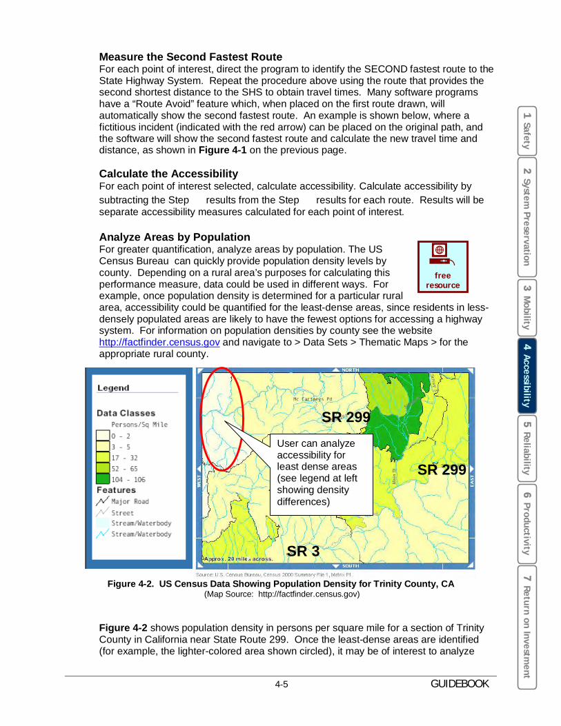
� Analyze Areas by Population For greater quantification, analyze areas by population. The US Census Bureau can quickly provide population density levels by county. Depending on a rural area’s purposes for calculating this free performance measure, data could be used in different ways. For resource example, once population density is determined for a particular rural area, accessibility could be quantified for the least-dense areas, since residents in less-densely populated areas are likely to have the fewest options for accessing a highway system. For information on population densities by county see the website http://factfinder.census.gov and navigate to > Data Sets > Thematic Maps > for the appropriate rural county.

SR 299

SR 3

SR 299

User can analyze accessibility for least dense areas (see legend at left showing density differences)

Figure 4-2. US Census Data Showing Population Density for Trinity County, CA (Map Source: http://factfinder.census.gov)

Figure 4-2 shows population density in persons per square mile for a section of Trinity County in California near State Route 299. Once the least-dense areas are identified (for example, the lighter-colored area shown circled), it may be of interest to analyze

1 Safety

4 Accessibility

2 System

Preservation 3

Mobility

5 Reliability

6 Productivity

7 Return on Investm

ent

4-5 GUIDEBOOK

http://factfinder.census.gov

http://factfinder.census.gov

accessibility for these areas by selecting several origins within these areas and checking the ability of motorists to reach the State Highway System using their fastest and second-fastest routes.


If a rural area has a GIS database available, Accessibility can be calculated for numerous points and even aggregated over the entire county or rural area. At present, most rural counties do not have GIS networks set up. At a minimum, for calculation of this measure, GIS data must include roadway and population layers.

1 Safety

4 Accessibility

2 System

Preservation 3

Mobility

5 Reliability

6 Productivity

7 Return on Investm

ent

4-6 GUIDEBOOK

Quick Reference

Accessibility

Performance Measures [units] § Accessibility Difference [min]: Time from a particular point between the

fastest and second-fastest routes to State Highway System access points.

InputsData Needed

Necessary As Feasible

Travel Times Between Fastest and Second-Fastest Routes from point(s) or communities of interest to the State Highway system using either: § Hard copy maps (easy to

analyze a few key points at no or little cost)

OR § Commercially available

software packages (minimal cost is under $100 at the time of this report, and most have the capability of calculating the shortest path automatically)

If GIS unavailable, use of U.S. Census data to facilitate further quantification of analysis

If available, GIS data and consisting of: § Critical local roads § State Highway System § Population layers from

Caltrans

Working with GIS software having analytic capability for shortest path algorithm

free resource

Posted speeds along the chosen routes to allow calculation of travel times

OutputsResults

Calculated

In order of increased resource availability (from hard copy maps and manual methods, to sophisticated GIS), outputs will consist of the following:

§ Accessibility for key points in the rural area

OR § Accessibility

for critical roads n the rural area

OR § Accessibility

aggregated for the entire rural area

4-7 GUIDEBOOK

1 Safety

4 Accessibility

2 System

Preservation 3

Mobility

5 Reliability

6 Productivity

7 Return on Investm

ent

Section 5 Reliability


Reliability refers to consistency or dependability of travel times and is a measure that compares expectations with experience. When considering reliability, the most important factors are being able to regularly and dependably predict travel time and avoid unexpected delay.

The performance measure for reliability might be of interest to a rural area if congestion is an issue or a growing issue in the area. Automated detection is necessary for cost-effectiveness in collecting a meaningful amount of roadway-related data for calculating reliability. For mass transportation services (bus and rail), service schedules are required.

Reliability can be measured across days, or across different times of the same day. Because a relatively large amount of data is needed for the performance measure calculation to be meaningful, reliability is most applicable to rural areas with automated detection and increasing congestion levels. Using probe vehicles for data collection is not cost efficient.

To quantify reliability, the suggested method is to divide the standard deviation of travel time by the average travel time. The result can then be displayed as a percentage. This percentage reflects the extent of variation in travel time during a chosen period from the average travel time during the same period. A high percentage reflects high variability in travel time because travel times are inconsistent. This might be due to accidents, re-occurring special events, or any other factor that causes travel time to vary in an unexpected fashion.

Given that a rural area has automated detection, reliability can be calculated manually using detector output, using a TDM, or using PeMS. PeMS itself is described further in the Technical Supplement. The requirements and procedure

free for transmitting data to the PeMS system are straightforward and will be resource described in more detail on page 5-4. Once an automated detector is connected to PeMS, several other performance measures can be calculated including those for productivity and mobility.

5 -1 GUIDEBOOK

1 Safety

5 Reliability

2 System

Preservation 3

Mobility

4 A

ccessibility 6

Productivity7


How Would a Rural Area Measure Reliability?

The methodology used depends on factors such as data availability, resources, and expertise. As resources increase or expertise improves, so will the ability to quantify reliability at an increasingly accurate level, where ‘increased accuracy’ may result in greater detail, greater geographical coverage, or increased sample size over different days depending on local needs. As with the other measures, the following step-by-step guidance is provided for two experience levels. For a rural area to be interested in measuring reliability, they would already have implemented automated detection to help manage their increasing congestion; thus, there is no basic level for this performance measure, only the intermediate and advanced levels.

If a rural area: Reliability measurement capabilities could be considered:

Reliability would be measured using:

§ Has automated detection Intermediate § Speeds (manual

processing is needed if § Only needs to compute travel times are being

reliability for a limited calculated from date range or for very speeds) few locations § Note: the process for

connecting to PeMS is straightforward and might be of benefit for future calculations

§ Has automated Advanced § PeMS output (gives detection variability for given

§ Needs to compute date range and time reliability over a large range from specified date range, and/or for detectors) followed by multiple corridors or minimal manual areas processing if necessary

§ Can transmit data to OR PeMS

AND/OR § TDM travel times § Uses a TDM output followed by

minimal manual processing if necessary

For urban and urbanizing areas periods of high traffic demand typically occur during weekday AM and PM peak periods, but in rural areas that experience high recreational demand, peak periods typically occur on weekends.

1 Safety

5 Reliability

2 System

Preservation 3

Mobility

4 A

ccessibility 6

Productivity7


5 -2 GUIDEBOOK


� Select Study Parameters Depending on a rural area’s intended purpose for calculating reliability performance measures, the roadways, roadway segments, times of day, and/or date range of interest must be carefully selected.

� Obtain Speeds from Detector Output Speeds must correspond with the study parameters outlined above.

� Calculate Travel Times Use speeds to calculate travel times.

Travel times can be computed by dividing the distance between the origin and destination by the average speeds:

Travel Time (in minutes) = Distance (in miles) x 60 / Speed (in miles per hour)

� Conduct Reliability Analysis Conduct reliability analysis using the following calculation: § For each OD pair specified in � above calculate the average travel time (whether

that is over several days, or over different times of day) § For each reading for each OD pair specified in � above calculate the standard

deviation (this is usually possible using a spreadsheet formula; for example, with Excel, the formula “STDEV” could be applied to that selected range)

§ Calculate a variability measure for each reading measured for the OD pair specified in � above using the following formula:

Variability (%) = Standard Deviation / Average Travel Time

A graph can also be used to indicate the corridors that experience the highest variability among the chosen corridors, or can be compared with additional graphs representing different time periods (for example, AM or PM) to show the corridors that experience the most variability and thus the least reliability. An example from data provided by the Southern California Association of Governments (SCAG) is presented in Figure 5-1. Data from a rural area was unavailable, thus this example from an urban area is shown to demonstrate the concept. Each data point (AM01, AM02, etc.) represents a different OD pair.

5 -3 GUIDEBOOK

3 M

obility 4

Accessibility

5 Reliability

6 Productivity

2 System

Preservation 7


1 Safety

Origin-Destination PairAM01

AM02

AM03

AM04

AM05

AM06

AM07

AM08

AM09

AM10

PM01

PM02

PM03

PM04

PM05

PM06

PM07

PM08

PM09

PM10

1 Safety

2 System

Preservation 3

Mobility

4 A

ccessibility 5

Reliability 6

Productivity7


Varia

bilit

y (P

erce

ntag

e ab

ove

aver

age

trave

l tim

e)

40%

35%

30%

25%

20%

15%

10%

5%

0%

This is OD Pair PM04, from 4-5 PM. Each dot within a group represents an hour during the peak period. Thus, this OD Pair shows the highest variability (therefore the lowest reliability) at this time (4-5 PM) within the peak period.

Origin-Destination Pair

AM Peak (6 AM to 8 AM) PM Peak (3 PM to 7 PM)

Figure 5-1: Example Reliability Results in District 7, Los Angeles

The example above shows the reliability of 20 OD pairs: 10 during the three-hour AM peak period (the measurement for each hour is indicated by the square point), and 10 during the four-hour PM peak period. The X-axis indicates the OD pair (all are designated ‘major’ by the SCAG travel demand model) and the peak period: AM or PM (e.g., AM02 is the second OD pair for the AM peak period). It is recognized that in rural areas, especially those with high recreational demand, peak periods often occur on weekends.

The Y-axis shows the variability of travel time by indicating the percentage above the average travel time for each OD pair. The travel time for PM04, for example (indicated in the diagram), varies the most during the second hour of the PM peak period (between 4 and 5 pm). Travelers who wish to minimize the chances of encountering unexpected delay could choose to make a trip at either an earlier or later time or select an alternative and more reliable route.


5 -4 GUIDEBOOK


To facilitate repeated analysis of corridors outfitted with automated detection, the use of PeMS should be considered. PeMS is the acronym for the Freeway Performance Measurement System Project. The Project, a joint effort by

free Caltrans, the University of California, Berkeley, and the Partnership for Advanced resource Technology on the Highways (PATH) involves the investigation of various freeway system performance measures. The software developed in conjunction with the PeMS project, is a web-based traffic data collection, processing and analysis tool used to assist in assessing the performance of the freeway system. PeMS extracts information from real-time and historical data and presents it in various forms to assist managers, traffic engineers, planners, freeway users, researchers, and traveler information service providers (value added resellers or VARs) with a variety of data and informational needs. The address of the PeMS website is http://pems.eecs.berkeley.edu/Public/.

� Contact PeMS Staff Regarding Connection of Rural Detectors to PeMS Contact information can be found at the PeMS website: http://pems.eecs.berkeley.edu/Public/. Staff can provide additional details and documentation regarding the integration requirements listed below.

� Gather Information About the Local Detector System Although agency representatives are guided through the integration process, PeMS staff requires information such as the following to begin: § Traffic data types collected - flow, occupancy, speed § Geospatial data - list of roadways, orientation (N., S., E., W.), and designation (State

road, arterial, etc.); and if desired, geographic regions (for example, a list of towns within the rural area if town name is an attribute); or postmiles or odometer readings from stations identified by latitude and longitude

§ Equipment configuration - complete identification of field elements such as controllers, stations, and detectors. Required and optional attributes can be explained by the PeMS staff

§ Configuration management - how to ensure that any changes to the above information will be communicated to PeMS

§ Data feeds - this is documentation about the data itself and can usually be provided by automated detector vendors

� Electronically Transmit Rural Area Detector Data to PeMS After the PeMS staff assists the rural area with connections and data compatibility issues, the rural area can then transmit detector data to PeMS directly.

� Apply for a Free PeMS Account Anyone is eligible to obtain a user account. Once logged in to a PeMS account online, the user can retrieve and manipulate the data of interest. All that is requested to obtain an account is name, phone, email address, agency name, and reason for use.

� Select Study Parameters Before logging into PeMS, study parameters such as roadways, roadway segments, times of day, and date range of interest should be chosen.

1 Safety

5 Reliability

2 System

Preservation 3

Mobility

4 A

ccessibility 6

Productivity7


5 -5 GUIDEBOOK

http://pems.eecs.berkeley.edu/Public

http://pems.eecs.berkeley.edu/Public

� Login and Obtain Outputs from PeMS Once logged into the PeMS, users may select a roadway segment of interest, and output travel times. The user may select date ranges, exclude certain days, and specify granularity (hours, days, etc.). In addition, the output can be viewed as a plot or table, and can be exported as text or an Excel file. In the example below, results were selected and displayed for Tuesdays between April 4, 2005 and April 4, 2006.

The following guidance is provided for navigating through the PeMS control panel (or “Dashboard”).

• select Routes > Travel Time > Time of Day > • select date range and days > • select Variability (to show the lower graph corresponding to the right axis,

which shows percent Variability).

� Analyze Variability For this one-year sample of Tuesdays only, the highest variability from the average travel time (indicated by the arrow) occurs at approximately 1:00 PM; thus, people traveling along this corridor at 1:00 PM experienced the highest unexpected delay for the selected one-year period. While the percent of variability shown for this corridor is quite small, results for different days and corridors will obviously differ.

The highest variability from the average travel time occurs at approximately 1:00 PM

Figure 5-2. Example PeMS Output for Reliability

� Export data to Excel for Further Analysis There is an “Export to XLS” feature which allows data to be automatically saved in spreadsheet format for further manipulation in Microsoft Excel.

1 Safety

5 Reliability

2 System

Preservation 3

Mobility

4 A

ccessibility 6

Productivity7


5 -6 GUIDEBOOK



Quick Reference

Reliability

Performance Measures [units] § Variability of travel times between major OD pairs

[% of standard deviation / average travel time]

Inputs Data Needed

Outputs Results

Calculated


Travel Times between major origin-destination pairs from: § automated detection, or § TDM output

Consider sending the input data to the California Freeway Performance Measurement System (PeMS), which will then process the data and provide the mobility measures recommended

Variability of travel times between major OD pairs [% of standard deviation / average travel time]

Can be measured over different days, or across different times of day

free resource

1 Safety

5 Reliability

2 System

Preservation 3

Mobility

4 A

ccessibility 6

Productivity7


5-7 GUIDEBOOK

Section 6 Productivity


The performance measure for productivity might be of value to a rural area if congestion is an issue or a potential issue in the area. Although many data collection methods are available, automated detection is the most cost-effective data collection method used in connection with this measure. Productivity is defined as the utilization of transportation system capacity. For roadways, capacity is defined as the maximum number of vehicles that a roadway can accommodate under prevailing roadway, traffic, and control conditions (HCM pg. 2.2). In other words, productivity measures how optimally the capacity of the system is used and how the system performs under high-traffic demand. For urban and urbanizing areas periods of high traffic demand typically occur during weekday AM and PM peak periods, but in rural areas that experience high recreational demand, peak periods typically occur on weekends. Productivity for roadways is an indicator of throughput and efficiency, where throughput is a measure of the actual number of vehicles or people that a roadway accommodates under prevailing roadway, traffic, and control conditions. During periods of congestion such as peak periods or when incidents occur, the amount of traffic that the roadway can accommodate may be reduced resulting in loss of productivity. Productivity can be measured system-wide, for a specific corridor or, for a specific roadway segment. The optimum measurement of system productivity is multi-modal, including rail, buses etc. and is typically determined by individual corridor.

How Would a Rural Area Measure Productivity?

The methodology used encompasses factors such as data availability, resources, and expertise. Productivity can be measured in terms of throughput or equivalent lost lane miles. Throughput refers to the flow or traffic volume that passes through a given point on the roadway. Equivalent Lost Lanes expresses the loss in freeway segment capacity resulting from vehicle back ups that reduce speeds and reduce throughput. When congestion occurs on a facility, throughput can decline dramatically and the roadway cannot serve as many vehicles as the number for which it is designed. The freeway or corridor section acts as a “smaller” or less effective facility, usually due to excessive merging and weaving. This can happen at an interchange with heavy traffic flowing onto the freeway from an on-ramp or another freeway, when an accident occurs that closes one or more lanes forcing significant merge activity (in other words, at bottleneck locations), or when a lane is dropped (for example, when it changes from five to four lanes). One “equivalent lost lane” on a five-lane freeway segment is equivalent to a twenty-percent reduction in capacity available to vehicles. (See the Technical Supplement for a more in-depth explanation of the Lost Lanes Concept.)

6 -1 GUIDEBOOK

3 M

obility 4

Accessibility

5 Reliability

6 Productivity

2 System

Preservation 7


1 Safety

As shown in the table below, the methodologies in this section would be considered by a rural area at an advanced level only because that area would have automated detection, and automated detection is required to calculate this performance measure due to the extensive traffic-related data collection effort required.

If a rural area: Productivity measurement capabilities could be considered:

Productivity would be measured using:

§ Has automated detection

§ Needs to compute this measure over a large date range, and/or for multiple corridors or areas

§ Can feed data to PeMS AND/OR § Uses a Travel Demand

Model

Advanced § PeMS output (gives variability for given date range and time range from specified detector(s)) followed by minimal manual processing if necessary

OR

§ TDM Travel Times output followed by minimal manual processing if necessary


Productivity can be measured in terms of throughput or equivalent lost lane miles. While throughput is typically used to measure the productivity of an individual roadway segment, the lost lane miles concept is used to measure system-wide productivity (across many roadway segments). The procedure to calculate throughput and lost lane miles is discussed in subsequent sections.

Throughput

Throughput can be computed by dividing the observed volumes on the roadway by the design roadway capacity, as shown in the following equation:

VT = C

Where:

T is the throughput in percent

C is the design roadway capacity, which for a two-lane rural highway, is 1,667 vehicles per hour per lane. The design capacity is based on the assumption that the terrain is

1 Safety

6 Productivity

2 System

Preservation 3

Mobility

4 A

ccessibility 5

Reliability 7


6 -2 GUIDEBOOK

level and that the vehicular traffic is comprised of 20% heavy truck volume. (Source: Highway Capacity Manual (HCM) 2000, Chapter 20)

V is the observed traffic volume in vehicles per hour per lane

Rural counties experiencing growing congestion would see increasing traffic volumes on the roadways. As traffic volumes increase, the eventual result will be roadways operating at full capacity. However, as demand increases, the actual number of vehicles served by the roadways tends to decrease due to increasing congestion caused by the inefficient use of the system. The result is lost productivity. At this stage, the roadway performs like a smaller or less effective facility than its design would indicate.

The following steps explain the procedure for calculating the productivity of a roadway under study in terms of throughput:

� Using a graph sheet, identify time of day on the x-axis and traffic volume (vehicles per hour per lane) on the y-axis,

� Using the Highway Capacity Manual (HCM) identify the capacity of the roadway under study (1,667 vehicles per hour per lane for a two-lane roadway), and draw a horizontal line on the graph indicating the capacity.

� Plot the traffic volume data obtained. o In congested conditions (meaning that the reason why throughput and speeds are

low are due to high traffic volumes), the area between the line representing capacity and the plotted traffic volumes is the lost productivity. This area is shown in Figure 6-1. If there are multiple days of data, for each volume (vehicles per hour) observation, either the average or the highest value can be used.

o If the traffic volume curve coincides with the capacity curve during certain periods of time, then it can be concluded that the roadway is operating at its full potential during those periods of time.

Figure 6-1. Illustration of Lost Productivity Concept

Lost Lane Miles

Productivity can also be measured in terms of lost lane miles. If losses in productivity are measured using lane miles, then lost productivity can be measured in terms of lost lane-miles of roadway. The following steps explain the procedure for calculating lost lane miles:

1 Safety

6 Productivity

2 System

Preservation 3

Mobility

4 A

ccessibility 5

Reliability 7


6 -3 GUIDEBOOK

3 M

obility 4

Accessibility

5 Reliability

6 Productivity

2 System

Preservation 7


1 Safety

� Multiply the number of lanes in each direction of the roadway by the length of the roadway segment. The number of lanes for a two-lane highway is one.

� From the observed 24-hour traffic volumes data (from ADT volumes), identify the one-hour traffic volume that represents the most congested condition. If more than one day of data is available, choose the lowest one-hour traffic volume from the available traffic volume data. It must be ensured that the low volume is due to congested conditions and not to actual low volumes themselves.

� Lost lane miles are calculated using the following formula:

V · n · ll = l -l c C

Where:

ll is lost lane miles

lc is the lane miles at capacity and is the product of n and l

V is the traffic volume in vehicles per hour per lane (vphpl)

n is the number of lanes on the roadway in one direction

l is the length of the roadway segment in miles

C is the design capacity in vehicles per hour per lane

In other words,

Lost lane miles = lane miles at capacity – (flow rate / capacity) [vphpl] X lanes X length of segment [mi]

This can be illustrated by the following example,

For a given a 1-lane roadway segment that is 4 miles in length, with an observed traffic volume of 1400 vphpl and a design capacity of 1667 vphpl:

Lane miles at capacity: 1 x 4 = 4 lane miles

Lost lane miles = 4 lane-mi - (1400/1667) x 1 lane x 4 mi = 4 - (0.84) x (1) x (4) = 4 – 3.36

= 0.64 lost lane miles

In other words, during the most congested period, 0.64 lane miles of roadway capacity were lost due to inefficient system usage. Lost lane miles for each roadway segment in the region can be calculated and added to obtain the region-wide lost lane miles. This lost lane miles quantity could also indicate the equivalent cost of lost productivity when it is multiplied by the cost of construction per mile of roadway.

6 -4 GUIDEBOOK

Quick Reference

Productivity Performance Measures [units]

§ Vehicle throughput [actual volume/capacity of roadway in %] § Lost lane miles § System wide (or) per roadway segment

InputsData Needed


Traffic Volumes:

Average Daily Traffic (ADT) volume data (time stamped) for 12-hour period. For rural areas, this period may occur on a weekend if recreational activity in the area indicates such an evaluation.

Traffic Volumes:

Average Daily Traffic (ADT) volume data (24-hour time stamped traffic volume data) spanning a reasonable sample of days

OutputsResults

Calculated

Lost productivity of the roadway – graphical results

The longer the time period for which data is collected and analyzed, the more informative the result

6 -5 GUIDEBOOK

1 Safety

6 Productivity

2 System

Preservation 3

Mobility

4 A

ccessibility 5

Reliability 7


Section 7 Return on Investment


Return on investment (ROI) communicates to decision makers the value the public can expect from planned investments. Although ROI is determined at the individual project level, results may be combined or rolled-up to estimate the overall impact of multiple projects. Many rural counties evaluate the cost-effectiveness of projects using forecast data and currently do not actively use the specific performance measures related to return on investment contained below including:

§ Life-cycle costs [dollars] § Life-cycle benefits [dollars] § Net present value [dollars] § Benefit/cost ratio [benefits divided by costs] § Rate of return on investment [percent return per year] § Project payback period [years] § Calculated benefits [dollars]

o Travel time savings o Vehicle operating cost savings o Accident cost savings o Emission cost savings

How Would a Rural Area Measure Return on Investment?

The performance measures listed above can be directly output from the California Life-Cycle Benefit/Cost Analysis Model (Cal-B/C). Cal-B/C is a spreadsheet-based tool developed by Caltrans used for preparing analyses of free both highway and transit projects. Users input data defining the type, scope, and resource cost of projects. The model then calculates the performance measures listed above. Cal-B/C is used for all state highway-related capital projects and has the capabilities for usage with projects involving public transit investments and many State Highway Operation and Protection Program (SHOPP) projects (rehabilitation, operational improvement and intelligent transportation systems or ITS). The model can be directly downloaded and the associated user documentation is accessible via the web at:

http://www.dot.ca.gov/hq/tpp/offices/ote/benefit_cost.htm

This model can be useful to rural counties that do not maintain travel demand models (TDM)s since it has Highway Capacity Manual (HCM) computation capabilities that estimate project benefits. It is understandable that for counties that do not have TDMs, computations are more difficult. For pavement rehabilitation investments, pavement management systems can derive the incremental costs of deferring maintenance, which can then be used as a proxy for cost effectiveness.

1 Safety

2 System

Preservation 3

Mobility

4 A

ccessibility 5

Reliability 6

Productivity7


7 -1 GUIDEBOOK

http://www.dot.ca.gov/hq/tpp/offices/ote/benefit_cost.htm

Cal-B/C has analytic capabilities for project types such as truck climbing lanes and passing lanes that might be of interest to some rural counties. It also provides the ability to estimate user benefits derived from pavement projects. For counties with increasing congestion, the model translates other measures such as delay and accidents into economic values in dollars and compares these monetized benefits with the costs of the projects. Rural counties that have TDMs can estimate the total ROI of their Regional Transportation Improvement Plan (RTIP) projects by computing total travel time with and without the RTIP investments and then rely on a tool such as Cal-B/C to derive the ROI.

Among the rural areas reviewed, there were none which already analyzed ROI using a standardized measurement; thus, this methodology would be considered the basic level.

If a rural area: Return on Investment measurement capabilities could be considered:

Return on Investment would be measured using:

§ Currently does not determine ROI using Travel Demand Models or other methods

Basic § The Cal-B/C Model or a similar method


Among the rural areas reviewed, there were none which already analyzed ROI using a standardized measurement; thus, this methodology would be considered the basic level. As the Cal-B/C model is a readily available, free tool that incorporates the necessary calculations and economic assumptions, it is described here in such a manner that it can be the first step for standardized ROI measurement for a rural area. Comprehensive and easy-to-follow documentation is available with the model.

� Download Cal-B/C and User Documentation The Cal B/C model and all user documentation can be downloaded from the web at http://www.dot.ca.gov/hq/tpp/offices/ote/benefit_cost.htm. Instructions are also included with the spreadsheet model itself.

� Input Values in the Green Cells Values are further explained in the instructions (first tab of the spreadsheet). The model is illustrated in Figure 7-1 on the following page.

1 Safety

2 System

Preservation 3

Mobility

4 A

ccessibility 5

Reliability 6

Productivity7


7 -2 GUIDEBOOK

http://www.dot.ca.gov/hq/tpp/offices/ote/benefit_cost.htm.

Figure 7-1. Cal-B/C Graphical User Interface (Source: Cal-B/C v3.2 User’s Guide)

� View and Modify Parameters Parameters may be viewed and modified by the user in the Parameters tab. Step-by-step calculations can be viewed for travel times, vehicle operating costs, accident costs, emissions, and net present value using the appropriate tabs. Outputs are provided automatically by the model and are summarized in the Results tab illustrated in Figure 7-2 on the following page.

1 Safety

2 System

Preservation 3

Mobility

4 A

ccessibility 5

Reliability 6

Productivity7


7 -3 GUIDEBOOK

Figure 7-2. Cal-B/C “Results” Tab (Source: Cal-B/C v3.2 User’s Guide)

7 -4 GUIDEBOOK

1 Safety

2 System

Preservation 3

Mobility

4 A

ccessibility 5

Reliability 6

Productivity7



3 M

obility 4

Accessibility

5 Reliability

6 Productivity

2 System

Preservation 1

Safety

Performance Measures [units] § Life-cycle costs [dollars] § Life-cycle benefits [dollars] § Net present value [dollars] § Benefit/cost ratio [benefits divided by costs] § Rate of return on investment [percent return per year] § Project payback period [years] § Calculated benefits [dollars]

o Travel time savings o Vehicle operating cost savings o Accident cost savings o Emission cost savings

InputsData Needed

OutputsResults

Calculated


Project data such as: § Speed § Volumes § Accident data

Facility characteristics such as: § Length of construction

period § Length of peak period § Truck percentage § Vehicle occupancy

Project cost data such as: § Initial costs § Maintenance/operating

and rehabilitation costs § Mitigation costs

Inputs from TDM (data forecasts reflecting project in place)

Performance measures listed above output from the Cal-B/C Model

free resource

Quick Reference 7


7 -5 GUIDEBOOK

Glossary

A Accessibility: The opportunity and ease of reaching desired destinations Advanced: Regular, frequent performance measurement using current tools and methods

B Basic: Little or no standardized performance measurement

C Caltrans: California Department of Transportation CHP: California Highway Patrol

G GIS: Geographic Information Systems; an information system that is used to input, store, retrieve, analyze, and output geographically referenced data or geospatial data GPS: Global Positioning System

H HPMS: Highway Performance Monitoring System, which is available through Caltrans, and which provides mileage information in the form of Daily Vehicle Miles of Travel (DVMT), and is in the process of collecting pavement condition information

I Intermediate: Somewhat standardized performance measurement, often using current tools and methods

L Lost-Lane Miles: The equivalent lost capacity which a roadway facility experiences due to congestion due to situations such as bottleneck locations or lane decreases

M Mobility: The ease or difficulty of traveling from an origin to a destination; the potential for movement, or the ability to travel from point A to point B

P PCI: Pavement Condition Index; a scale from 0-100 that rates the condition of a roadway based on the amount of different distress types present PeMS: Caltrans Freeway Performance Measurement System; a web-based traffic data collection, processing, and analysis tool to assist traffic engineers in assessing the performance of the freeway system Performance Measure: A method to objectively measure the degree of success a program has had in achieving its objectives and goals PMS: Pavement Management System Productivity: The maximization of throughput or efficiency (system-wide); how well the capacity of the system is being used and how the system is performing under high traffic demand conditions

R Reliability: The consistency or dependability of travel times Return on Investment: Benefit-cost analysis or best return on investment (includes life-cycling costing) RTIP: Regional Transportation Improvement Program RTPA: Regional Transportation Planning Agency

S Safety: Reduce fatalities, injury, and property loss of system users and workers. STIP: Statewide Transportation Improvement Program SWITRS: Statewide Integrated Traffic Records System; a compilation of all reported roadway incidents received from CHP and local police and sheriffs System Preservation: Preservation of the publicly-owned transportation system at a specified state-of-repair or condition; physical condition of the system

T TASAS: Traffic Accident and Surveillance Analysis System; tracks detailed information pertaining to State Highway related incidents using an accident database and a highway database TDM: Travel Demand Model

Performance Measures for Rural Transportation … Measures for Rural Transportation Systems...

Documents

Transcript of Performance Measures for Rural Transportation … Measures for Rural Transportation Systems...