Bahaddin M. Abubakr, Osama A. Abolaeha, Alamin A. Hameda

Department of Electrical & Electronic Engineering University of Tripoli, Tripoli, Libya

Baha.mousa91@gmail.com

Abstract : Various tuning methods have been proposed for proportional-integral-derivative (PID) controller. A respectively new and simple experimental method for tuning PID controllers named a Good Gain method that was recently proposed by F. Haugen in 2010, this method is not yet recognized among the other known methods for tuning. However, the founder of this methods claims that it can be an alternative to the famous Ziegler-Nichols. In this paper, PID tuning method has been performed experimentally using a real water level system in order to test and validates the Good Gain method. Also other PID tuning methods applied to the same system to compare the results. The results show that the Good Gain method gives an acceptable stability and response comparing to the other industrial PID controller tuning procedures. Keyworlds: PID tuning methods; Ziegler–Nichols method; Good Gain method; Control Systems

Ι. INTRODUCTION Since 1930s three mode controllers with PID

actions became commercially available and gained success in practical applications. These types of controllers are still the most widely used in industrial application. In order to find an accurate PID parameters is by knowing the process’s mathematical model. But sometimes the process is very complicated, therefore, finding its model will be difficult. As a result of this problem, other tuning procedures have been proposed to find the parameters of PID of a process without dealing with the mathematical model. These procedures offering an acceptable controlling response based on the stability and low error also rejecting disturbances. These different approaches are called tuning methods and they are classified into:

Firstly, the Open-loop procedures which refer to methods that tune the controller when it’s on manual mode and the process runs in an Open-loop mode. Open-loop methods are: Open-loop Ziegler-Nichols method, C-H-R method, Cohen and Coon method, Fertik method, Ciancone-Marline method, IMC method and Minimum error criteria (IAE, ISE, ITAE) method [2].

Secondly, the Closed-loop tuning procedures which refer to methods that tune the controller during automatic mode when the process is running in Closed-loop mode. The Closed-loop methods that are involved in this experiment study are: The Good Gain method, Ziegler-Nichols method, Modified Ziegler-Nichols method and Tyreus-Luyben Method [2, 3, 4].

The Good Gain method as all the other methods it can be applied to real processes without any priority information about the process model and what’s make it unique is its ease of use . The method was first presented by Haugen in 2010 [1], but the theoretical rationale paper was published in 2012 [5]. And Haugen experiments the method on temperature control systems. Also this paper demonstrate a comparison of the performances of the Good Gain method to other industrial tuning methods. As, Haugen suggests to compare the Good Gain method with different process other than temperature control systems [6].

ΙΙ. THE EXPERIMENTAL SETUP The physical system used in the experiments is

the Level Process Trainer manufactured by Festo Didactic as shown in Figure 1. The water level in the tank is controlled by adjusting the control signal that operate the water pump and control the water flow that enters the tank. The tank mounted on the work surface it has four ports, two ports on the top and the other two are in the bottom. One of the ports which are located on the top is connected to the pipe that coming from the pumping unit to flow water into the tank and the other one is used to return the water to the reservoir in case of an overflow. One of the ports which are located on the bottom is connected to the pipe to out the flow to the reservoir and the other one is connected to a hand operated valve that works as a disturbance, hence, the operator can apply a sudden change in the outflow as an act of disturbance input, this will show how the controller reacts and how the control signal modify itself when the disturbance occur.

A deferential pressure transmitter is used as a water level sensor, level sensing with pressure sensors can be performed by measuring relative pressure, for example, pressure P1 is equal to ambient pressure and pressure P2 to ambient pressure plus the pressure generated by the weight of the liquid column (hydrostatic pressure). The equation that relates the level of liquid in a vessel, h, to the hydrostatic pressure of the liquid 𝑃𝑔, is as follows: h= (Pg ×1000 Pa/KPa)/(ρ ×g) (1)

Figure 1: The level process trainer with the pumping unit

Performance Evaluation of the Good Gain Method Against Other Methods Using a Water Level

Control System

INTERNATIONAL JOURNAL OF SYSTEMS APPLICATIONS, ENGINEERING & DEVELOPMENT DOI: 10.46300/91015.2020.14.8 Volume 14, 2020

ISSN: 2074-1308 44

Where h represents the level of the liquid (m), 𝑃𝑔 is hydrostatic pressure of the liquid (kPa, gauge), ρ gives the mass density of the liquid (kg/m3), and g is gravitational acceleration (m/s2). The equation shows that the level of the liquid varies in direct proportion to the hydrostatic pressure of the liquid. This direct relationship is true provided that the temperature and the density of the liquid remain constant in the vessel.

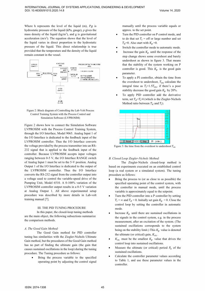
Figure 2: Block diagram of Controlling the Lab-Volt Process Control Training System with the Process Control and

Simulation Software (LVPROSIM)

Figure 2 shows how to connect the Simulation Software LVPROSIM with the Process Control Training System, through the I/O Interface, Model 9065. Analog Input 1 of the I/O Interface is dedicated to the feedback input of the LVPROSIM controller. Thus the I/O Interface converts the voltage provided by the process transmitter into an RS-232 signal that is applied to the feedback input of the controller. Because LVPROSIM accepts input voltages ranging between 0-5 V, the I/O Interface RANGE switch of Analog Input 1 must be set to the 5-V position. Analog Output 1 of the I/O Interface is dedicated to the output of the LVPROSIM controller. Thus the I/O Interface converts the RS-232 signal from the controller output into a voltage used to control the variable-speed drive of the Pumping Unit, Model 6510. A 0-100% variation of the LVPROSIM controller output results in a 0-5 V variation at Analog Output 1. All above experimented setup procedure was described by more details in Lab-volt training manual [7].

III. THE PID TUNING PROCEDURE In this paper, the closed-loop tuning methods

are the main object, the following subsections summarize the comparison methods. A. The Good Gain Method:

The Good Gain method for PID controller tuning has similarities with the Ziegler-Nichols Ultimate Gain method, but the procedures of the Good Gain method has no part of finding the ultimate gain (the gain that causes sustained oscillations in the loop) during the tuning procedure. The Tuning procedure as follows:

Bring the process variable to the specified operating point by adjusting the control signal

manually until the process variable equals or approx. to the set point.

Turn the PID controller on P control mode, and to do that set 𝑇𝑖 = off or large number and set 𝑇𝑑=0. Also start with 𝐾𝑝 =0.

Switch the controller mode to automatic mode. Increase the gain 𝐾𝑝 until the response of the

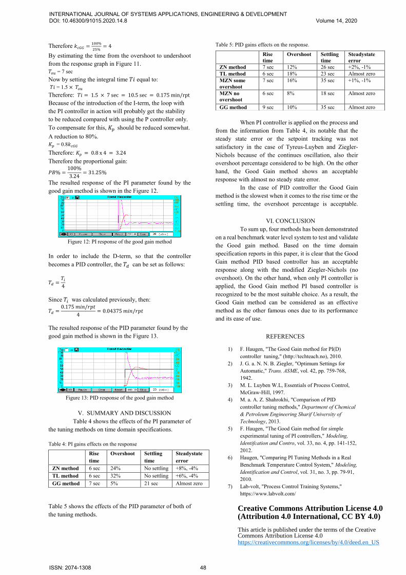
step change shows some overshoot and barely undershoot as shown in figure 3. That means that the stability of the system working on P controller is good. This 𝐾𝑝 is the good gain parameter.

To apply a PI controller, obtain the time from the overshoot to undershoot, 𝑇𝑜𝑢 calculate the integral time as 𝑇𝑖=1.5𝑇𝑜𝑢, if there’s a poor stability decrease the good gain 𝐾𝑝 by 20%.

To apply PID controller add the derivative term, set 𝑇𝑑=𝑇𝑖/4 (which is the Ziegler-Nichols Method ratio between 𝑇𝑑 and 𝑇𝑖).

Figure 3: the time from the overshoot to undershoot 𝑇𝑜𝑢

B. Closed Loop Ziegler-Nichols Method:

The Ziegler-Nichols closed-loop method is based on experiments executed on an established control loop (a real system or a simulated system). The tuning procedure as follows: Bring the process to (or as close to as possible) the

specified operating point of the control system, with the controller in manual mode, until the process variable is approximately equal to the setpoint.

Turn the PID controller into a P controller by setting 𝑇𝑖 = ∞ and 𝑇𝑑 = 0. Initially set gain 𝐾𝑝 = 0. Close the control loop by setting the controller in automatic mode.

Increase 𝐾𝑝 until there are sustained oscillations in the signals in the control system, e.g. in the process measurement, after an excitation of the system. (The sustained oscillations corresponds to the system being on the stability limit.) This 𝐾𝑝 value is denoted the ultimate (or critical) gain, 𝐾𝑐𝑢 .

𝐾𝑐𝑢 must be the smallest 𝐾𝑝 value that drives the control loop into sustained oscillations.

Measure the ultimate (or critical) period 𝑃𝑢 of the sustained oscillations.

Calculate the controller parameter values according to Table 1, and use these parameter values in the controller.

INTERNATIONAL JOURNAL OF SYSTEMS APPLICATIONS, ENGINEERING & DEVELOPMENT DOI: 10.46300/91015.2020.14.8 Volume 14, 2020

ISSN: 2074-1308 45

Table 1: Ziegler-Nichols Controller Parameters Table Controller 𝑲𝒑 𝑻𝒊 𝑻𝒅

P 0.5𝐾𝑐𝑢

PI 0.45𝐾𝑐𝑢 𝑃𝑢/1.2

PID 0.6𝐾𝑐𝑢 𝑃𝑢/2 𝑃𝑢/8

C. Modified Ziegler-Nichols Method:

For some control loops the measure of oscillation, provide by ¼ decay ratio and the corresponding large overshoots for set point changes are undesirable therefore more conservative methods are often preferable such as modified Z-N settings These modified settings is giving in Table 2 for some overshoot and no overshoot. Table 2: Modified-Ziegler-Nichols Controller Parameters Table

Controller 𝑲𝒑 𝑻𝒊 𝑻𝒅 Some overshoot

0.33𝐾𝑐𝑢 𝑃𝑢/2 𝑃𝑢/3

No overshoot 0.2𝐾𝑐𝑢 𝑃𝑢/2 𝑃𝑢/8 D. Tyreus-Luyben Method:

The Tyreus-Luyben method is quite similar to the famous Ziegler-Nichols closed-loop method, the method procedure is the same steps 1 to 5 of Ziegler-Nichols closed loop method. Step 5 Evaluate the control parameters as presented by Tyreus-Luyben is giving in Table 3.

Table 3: Tyreus-Luyben Controller Parameters Table

Controller 𝑲𝒑 𝑻𝒊 𝑻𝒅

PI 𝐾𝑐𝑢/3.2 2.2𝑃𝑢 PID 𝐾𝑐𝑢/2.2 2.2𝑃𝑢 𝑃𝑢/6.3

IV. CONTROLLER TUNINGS AND RESULTS

After all the proper connections of the process, the tuning of the PID controller was done based on the tuning procedures that was described in the above section, the aim is to calculate PID parameters that give satisfying response, also to minimize the error as possible and to reject the sudden disturbances. A. Ziegler-Nichols closed-loop method results:

First method applied on the process level trainer is the famous Ziegler-Nichols Closed-Loop Tuning Method. By following its procedure steps. The software LVPROSIM is working with a PID algorithm that work with the proportional band instead of the proportional gain. The proportional band relation to the proportional gain is given by: 𝑃𝐵% =

100

𝐾𝑝 (3)

In order to increase Kp to get a sustained oscillations of the process variable signal. The operator must decrease 𝑃𝐵%. Also the operator should turn the Ti off and set Td to zero, in order to illuminate their action.

By decreasing the 𝑃𝐵% value a sustained oscillations is found in the level as shown in the Figure 4. The 𝑃𝐵% value that made the response is: 𝑃𝐵% = 2 %. Therefore: Kcu = 100%

2 % = 50

Figure 4: Continues oscillation response

From the readings on the scale, the ultimate period is Pu = 8.6 sec. The calculations of Ziegler-Nichols PI and PID parameters can be found based on Table 1 formulas.

Calculating the parameter of PI and PID controllers Firstly, PI control mode: 𝐾𝑝 = 0.45𝐾𝑐𝑢 = 0.45 × 50 = 22.5 Therefore the 𝑃𝐵% =

100%

22.5= 4.44%

𝑇𝑖 =𝑃𝑢

1.2=

8.6 𝑠𝑒𝑐

1.2= 7.1667 𝑠𝑒𝑐

Therefore the 𝑇𝑖 = 7.1667 𝑠𝑒𝑐

60= 0.12 𝑚𝑖𝑛/𝑟𝑝𝑡

The resulted response after applying the calculated PI parameters is shown in Figure 5.

Figure 5: PI response of the Close-loop Ziegler-Nichols method

Secondly, PID Control Mode:

𝐾𝑝 = 0.6𝐾𝑐𝑢 = 0.6 × 50 = 30 Therefore the 𝑃𝐵% =

100%

30= 3.33%

𝑇𝑖 =𝑃𝑢

2=

8.6 𝑠𝑒𝑐

2= 4.3 𝑠𝑒𝑐

Therefore 𝑇𝑖 =4.3 𝑠𝑒𝑐

60= 0.071667 𝑚𝑖𝑛/𝑟𝑝𝑡

𝑇𝑑 =𝑃𝑢

8=

8.6 𝑠𝑒𝑐

8= 1.075 𝑠𝑒𝑐

Therefor the 𝑇𝑑 =1.075 𝑠𝑒𝑐

60= 0.018 𝑚𝑖𝑛/𝑟𝑝𝑡

The resulted response after applying the calculated PI parameters is shown in Figure 6.

Figure 6: PID response of the close loop Ziegler-Nichols

method

INTERNATIONAL JOURNAL OF SYSTEMS APPLICATIONS, ENGINEERING & DEVELOPMENT DOI: 10.46300/91015.2020.14.8 Volume 14, 2020

ISSN: 2074-1308 46

B. Modified Ziegler-Nichols Methods results: After applying the classic Ziegler-Nichols, and since the Modified Ziegler-Nichols method uses the same findings as the classic, therefore, the findings can be applied to find the PI and PID parameter based on Table 2 formulas.

Calculating the parameter of PID controller Firstly, with some overshoot:

𝐾𝑝 = 0.33𝐾𝑐𝑢 = 0.33 × 50 = 16.5 Therefore the 𝑃𝐵% =

100%

16.5= 6.0606%

𝑇𝑖 =𝑃𝑢

2=

8.6 𝑠𝑒𝑐

2= 4.3 𝑠𝑒𝑐

Therefore the 𝑇𝑖 =4.3 𝑠𝑒𝑐

60= 0.071667 𝑚𝑖𝑛/𝑟𝑝𝑡

𝑇𝑑 =𝑃𝑢

3=

8.6 𝑠𝑒𝑐

3= 2.8667 𝑠𝑒𝑐

Therefore the 𝑇𝑑 =2.8667 𝑠𝑒𝑐

60= 0.0477 𝑚𝑖𝑛/𝑟𝑝𝑡

The resulted response after applying the calculated PID parameters is shown in the Figure 7.

Figure 7: PID response of the Some Overshoot Modified-Ziegler-Nichols method

Secondly, no overshoot:

𝐾𝑝 = 0.2𝐾𝑐𝑢 = 0.2 × 50 = 10 Therefore the 𝑃𝐵% =

100%

10= 10%

𝑇𝑖 =𝑃𝑢

2=

8.6 𝑠𝑒𝑐

2= 4.3 𝑠𝑒𝑐

Therefore the 𝑇𝑖 =4.3 𝑠𝑒𝑐

60= 0.071667 𝑚𝑖𝑛/𝑟𝑝𝑡

𝑇𝑑 =𝑃𝑢

8=

8.6 𝑠𝑒𝑐

8= 1.075𝑠𝑒𝑐

Therefore the 𝑇𝑑 =1.075 𝑠𝑒𝑐

60= 0.018 𝑚𝑖𝑛/𝑟𝑝𝑡

The resulted response after applying the calculated PID parameters is shown in the Figure 8.

Figure 8: PID response of the No Overshoot Modified-Ziegler-

Nichols method

C. Tyreus-Luyben Method results:

Since this method has the same steps of the Ziegler-Nichols Closed-Loop Tuning Method. Then it has the same ultimate period with the same 𝐾𝑐𝑢. Now by calculation the Tyreus-Luyben PI and PID parameter can be found based on Table 3 formulas.

Calculating the parameter of PI and PID controller Firstly, PI control mode:

𝐾𝑝 =𝐾𝑐𝑢

3.2=

50

3.2= 15.625

Therefore the 𝑃𝐵% =100%

15.625= 6.4%

𝑇𝑖 = 2.2𝑃𝑢 = 2.2 × 8.6 = 18.92 𝑠𝑒𝑐 Therefore 𝑇𝑖 =

18.92 𝑠𝑒𝑐

60= 0.31533 𝑚𝑖𝑛/𝑟𝑝𝑡

The resulted response after applying the calculated PI parameters is shown in the Figure 9.

Figure 9: PI response of the Tyreus-Luyben method

Secondly, PID control mode:

𝐾𝑝 =𝐾𝑐𝑢

2.2=

50

2.2= 22.7272

Therefore the 𝑃𝐵% =100%

22.7272= 4.4%

𝑇𝑖 = 2.2𝑃𝑢 = 2.2 × 8.6 = 18.92 𝑠𝑒𝑐 Therefore the 𝑇𝑖 =

18.92 𝑠𝑒𝑐

60= 0.31533 𝑚𝑖𝑛/𝑟𝑝𝑡

𝑇𝑑 = 𝑃𝑢

6.3=

8.6

6.3= 1.36508 𝑠𝑒𝑐

Therefore the 𝑇𝑑 =1.36508 𝑠𝑒𝑐

60= 0.02275𝑚𝑖𝑛/𝑟𝑝𝑡

The resulted response after applying the calculated PID parameters is showing in the Figure 10.

Figure 10: PID response of the Tyreus-Luyben method

D. The Good Gain Method:

This method was described in section 3, it uses the same principles as the Ziegler-Nichols method, by turning the 𝑇𝑖 off and setting 𝑇𝑑 to zero and applying increase or decrease on 𝐾𝑝 value until the slight overshoot is observed. In the LVPROSIM a decreasing on the PB% value is done until the response shown in the Figure 11 occurred. In order to calculate the time between the over shoot and the under shoot. The Proportional gain that is responsible for this response is called kcGG.

Figure 11: Reading off the time 𝑇𝑜𝑢

The proportional gain that made the response of the above figure is PB% = 25 %.

INTERNATIONAL JOURNAL OF SYSTEMS APPLICATIONS, ENGINEERING & DEVELOPMENT DOI: 10.46300/91015.2020.14.8 Volume 14, 2020

ISSN: 2074-1308 47

Therefore 𝑘𝑐𝐺𝐺 =100%

25%= 4

By estimating the time from the overshoot to undershoot from the response graph in Figure 11. 𝑇𝑜𝑢 = 7 sec Now by setting the integral time 𝑇𝑖 equal to: 𝑇𝑖 = 1.5 × 𝑇𝑜𝑢 Therefore: 𝑇𝑖 = 1.5 × 7 sec = 10.5 sec = 0.175 min/rpt Because of the introduction of the I-term, the loop with the PI controller in action will probably get the stability to be reduced compared with using the P controller only. To compensate for this, 𝐾𝑝 should be reduced somewhat. A reduction to 80%. 𝐾𝑝 = 0.8𝑘𝑐𝐺𝐺 Therefore: 𝐾𝑝 = 0.8 x 4 = 3.24 Therefore the proportional gain:

𝑃𝐵% =100%

3.24= 31.25%

The resulted response of the PI parameter found by the good gain method is shown in the Figure 12.

Figure 12: PI response of the good gain method

In order to include the D-term, so that the controller becomes a PID controller, the 𝑇𝑑 can be set as follows:

𝑇𝑑 =𝑇𝑖

4

Since 𝑇𝑖 was calculated previously, then:

𝑇𝑑 =0.175 𝑚𝑖𝑛/𝑟𝑝𝑡

4= 0.04375 𝑚𝑖𝑛/𝑟𝑝𝑡

The resulted response of the PID parameter found by the good gain method is shown in the Figure 13.

Figure 13: PID response of the good gain method

V. SUMMARY AND DISCUSSION Table 4 shows the effects of the PI parameter of the tuning methods on time domain specifications.

Table 4: PI gains effects on the response

Table 5 shows the effects of the PID parameter of both of the tuning methods.

Table 5: PID gains effects on the response.

When PI controller is applied on the process and from the information from Table 4, its notable that the steady state error or the setpoint tracking was not satisfactory in the case of Tyreus-Luyben and Ziegler-Nichols because of the continues oscillation, also their overshoot percentage considered to be high. On the other hand, the Good Gain method shows an acceptable response with almost no steady state error. In the case of PID controller the Good Gain method is the slowest when it comes to the rise time or the settling time, the overshoot percentage is acceptable.

VI. CONCLUSION

To sum up, four methods has been demonstrated on a real benchmark water level system to test and validate the Good gain method. Based on the time domain specification reports in this paper, it is clear that the Good Gain method PID based controller has an acceptable response along with the modified Ziegler-Nichols (no overshoot). On the other hand, when only PI controller is applied, the Good Gain method PI based controller is recognized to be the most suitable choice. As a result, the Good Gain method can be considered as an effective method as the other famous ones due to its performance and its ease of use.

REFERENCES

1) F. Haugen, "The Good Gain method for PI(D) controller tuning," (http://techteach.no), 2010.

2) J. G. a. N. N. B. Ziegler, "Optimum Settings for Automatic," Trans. ASME, vol. 42, pp. 759-768, 1942.

3) M. L. Luyben W.L, Essentials of Process Control, McGraw-Hill, 1997.

4) M. a. A. Z. Shahrokhi, "Comparison of PID controller tuning methods," Department of Chemical & Petroleum Engineering Sharif University of Technology, 2013.

5) F. Haugen, "The Good Gain method for simple experimental tuning of PI controllers," Modeling, Identifcation and Contro, vol. 33, no. 4, pp. 141-152, 2012.

6) Haugen, "Comparing PI Tuning Methods in a Real Benchmark Temperature Control System," Modeling, Identification and Control, vol. 31, no. 3, pp. 79-91, 2010.

7) Lab-volt, "Process Control Training Systems," https://www.labvolt.com/

Rise time

Overshoot Settling time

Steadystate error

ZN method 6 sec 24% No settling +8%, -4% TL method 6 sec 32% No settling +6%, -4% GG method 7 sec 5% 21 sec Almost zero

Rise time

Overshoot Settling time

Steadystate error

ZN method 7 sec 12% 26 sec +2%, -1% TL method 6 sec 18% 23 sec Almost zero MZN some overshoot

7 sec 16% 35 sec +1%, -1%

MZN no overshoot

6 sec 8% 18 sec Almost zero

GG method 9 sec 10% 35 sec Almost zero

Creative Commons Attribution License 4.0 (Attribution 4.0 International, CC BY 4.0)

This article is published under the terms of the Creative Commons Attribution License 4.0 https://creativecommons.org/licenses/by/4.0/deed.en_US

INTERNATIONAL JOURNAL OF SYSTEMS APPLICATIONS, ENGINEERING & DEVELOPMENT DOI: 10.46300/91015.2020.14.8 Volume 14, 2020

ISSN: 2074-1308 48