PERFORMANCE CHARACTERISTICS OF AI •SPACED LOOP ANTENNA FORMED BY

I o1l • TWO ARBITRARILY ORIENTEDPARALLEL LOOPS

o •-

111 DDC

cm ~JUN 24 IV6

TISLABa

Submitted as Task Summary Report Number XIII. Also submitted asan Interim Development Report covering the period 1 January 1963 to

1 April 1963. Prepared for Navy Department, Bureau of Ships,

Electronics Division, Contract Nr. NObsr-89167, Project Ser. Nr.SF 0010801, Task 9Z58, Date of Report, 1 April 1963. Prepared byDouglas N. Travers.1SOUTHWES'T RESEARCH INSTITUTE

I SAN ANTONIO, TEXAS

t PERFORMANCE CHARACTERISTICS OF A

I SPACED LOOP ANTENNA FORMED BYTWO ARBITRARILY ORIENTED

PARALLEL LOOPS

I

Submitted as •ajk S nary__• Also submitted as

an Qýrim D)eVel_ S3 nt v e 3n~ ei an~I AprM Prepared for Navy Department, Bureau 0•f{ip, •

-V nin:ontractgo* j(,• .,SF 000801•l(Task 9Z5• Date'"'o eport.,l AprW63 3

,Irepa ....y(. \ APPROVED:

I~ ~~N Traverss ManagerW.LeRadio Direction Finding Research -

I DW. yle-Donaldson, Directorlilt Electronics and Electrical

S 0 Engineering

. '" UTHWEST RESEARCH INSTITUTESAN ANTONIO, TEXAS

LI! ABSTRACT

The spaced loop antenna is of interest in HF-DF because of itssuperior performance relative to the simple loop with respect to bearingaccuracy when reradiating objects are nearby. The shipboard site is aprime example. It is therefore of interest to study in some detail othercharacteristics of the spaced loop particularly those which are inferiorto the simple loop, such as sensitivity.

\rhis report lrRl7evn prepared in order to make available in asingle reference a complete listing of the important performance character-istics of the spaced loop antenna. The exact field equations of a generalspaced loop are derived and used as a basis for all other performancecharacteristics. The coaxial spaced loop and coplanar spaced loop aretreated as special cases of the general analysis. Any two loop spacedloop operating in the quadrupole mode may be treated as a special case.

Field patterns are derived for near and far fields, for azimuthand elevation planes, and for both vertical and horizontal polarization,for any spaced loop. These results are plotted to show that certainspaced loops have pattern variations as a function of distance to the source.The field equations are then used to compute the radiation resistance, theeffective height, effective area, gain, signal-to-noise ratio, noise figure,minimum observable field strength and impedance. Other characteristicsincluding reradiation error reduction, pattern variations with sourcedistance, construction difficulties and pattern distortion sources arereviewed. Although the report begins with ii- general concepts GeQfl~yrtfiga spaced loop, all important formulas are explained with numerical examplesso-6ht• practical conclusions may be drawn. I

Interim period activities are summa ized in the last section of thereport.

Iii

Ii

1. Introduction to the Problem of the Spaced ioop 1

2. Types of Spaced Loops 2

3. Equivalence of the Loop Antenna and a Magnetic Dipole 4

4. Mathematical Basis for Derivation of the FieldEquations 5

5. The Electric Field Components for the General SpacedLoop 9

6. The Magnetic Field Components for the General SpacedLoop 13

7. The Electric Field Components for the Simple LoopSense Antenna 17

8. The Magnetic Field Components for the Simple LoopSense Antenna 20

9. Summary Tables of the Field Equations 22

10. Combinations of Spaced Loop and Simple LoopAntennas 28

11. Effective Height of the Spaced Loop 31

12. Radiation Resistance of the Spaced Loop 34

13. Gain of the Spaced Loop 36

14. Effective Area of the Spaced Loop 38

15. Signal-to-Noise Ratio of the Spaced Loop Antenna 40

16. Minimum Observable Field Strengths 45

iii

II

TABLE OF CONTENTS (Cont'd)

Page

17. Impedance of the Spaced Loop Antenna 50

18. Other Spaced Loop Characteristics 52

19. Comparison with Equivalent Factors for the SimpleLoop 57

20. Conclusions 59

21. Bibliography of Spaced Loop Reports and Papers 62

22. Activities for the Interim Period 66

Ii

I..

I.

1.

iv

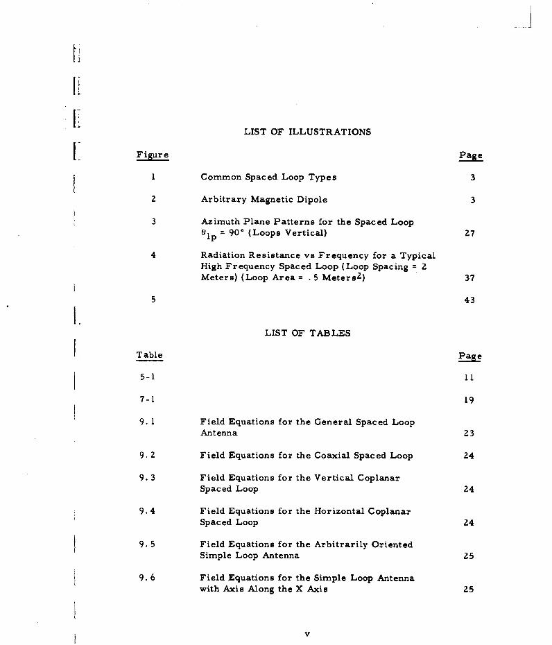
IiLIST OF ILLUSTRATIONS

Figure Page

I Common Spaced Loop Types 3

2 Arbitrary Magnetic Dipole 3

3 Azimuth Plane Patterns for the Spaced Loopalp = 90° (Loops Vertical) 27

4 Radiation Resistance vs Frequency for a TypicalHigh Frequency Spaced Loop (Loop Spacing = 2Meters) (Loop Area = . 5 Meters 2 ) 37

5 43I!.LIST OF TABLES

Table Page

5-1 11

7-1 19

9. 1 Field Equations for the General Spaced LoopAntenna 23

9.2 Field Equations for the Coaxial Spaced Loop 24

9.3 Field Equations for the Vertical CoplanarSpaced Loop 24

9.4 Field Equations for the Horizontal CoplanarSpaced Loop 24

9.5 Field Equations for the Arbitrarily OrientedSimple Loop Antenna 25

9.6 Field Equations for the Simple Loop Antennawith Axis Along the X Axis 25

V

1- LIST OF TABLES (Cont'd)

Table Page

L 9.7 Field Equations for the Simple Loop Antennawith Axis Along the Y Axis 25

9.8 Field Equations for the Simple Loop Antennawith Axis Along the Z Axis 25

9.9 Short Electric Dipole (Along Z Axis) 25

I-

I.

vi

Ii]

1 Introduction to the Problem of the Spaced Loop

Spaced loop radio direction finding antennas have been frequentlyproposed and occasionally used since the early days of radio. Friis Iconstructed and tested an elaborate coplanar spaced loop prior to 1925.Many coaxial types have been developed since that time2- 6 .

In most instances far field patterns have been derived or measuredand shown to possess certain desirably characteristics, including improvedL directivity over a simple loop.

In this report two fundamentally important characteristics of thespaced loop are considered in detail as they affect the designer. Theseare (1) variations in the field pattern as the source (or point of observation)is moved from the near to the far field region of the antenna, that is, fromr << X to r >5 X, and (2) factors which determine the signal-to-noise ratioof the spaced loop in a practical receiving system.

1. Friis, H. T., "A New Directional Receiving System, " Proc. IRE,Vol. 13, December 1925, pp. 685-707. "

2. "Instruction Book for Navy Model DAB-3 Radio Direction FinderEquipment," Collins Radio Company, NAVSHIPS 95073, 10 December 11942.

3. Crampton, C., "A Note on the Application of Spaced Loop High Fre-quency Direction Finder in H. M. Ships, " Report M. 433, DirectionFinder Section, Admiralty Signal Establishment, July 1942.

4. Travers, Douglas N., "A New Shipboard Direction Finding Antennafor the Reduction of Reradiation Error, " Southwest Research Institute,1 September 1960.

5. Travers, Douglas N., et al. "A Method of Goniometer Scanning theCoaxial Spaced Loop Direction Finder for Vertical Polarization, "Task Summary Report VIII, Southwest Research Institute, 1 April 1961.

6. Evans, G., "The Crossed-Spaced-Loop Direction-Finder Aerial,"IRE Transactions on Antennas and Propagation, .Vol. AP-10 Number6, November 1962, pp. 686-691.

2

It is shown that certain spaced loops have a radiation pattern whichis a function of the distance to the source or point of observation. Further-more multimode arrangements, such as Use of a simple loop in conjunctionwith a spaced loop, always produce a pattern which is a function of distance

I. to the source. As a result analyses based on far field patterns may lead toerroneous conclusions concerning the effect of nearby sources (near fieldsources less than one wavelength away) such as shipboard reradiators.

In another section of this report, Fatterns are derived some ofwhich have been experimentally verified.' Criteria for avoiding the variousdifficulties are given and near field testing procedures outlined. It isconcluded that in general one should not attempt to design a spaced loop ormultimode loop array for use when both near and far field sources may beof interest (as for instance an HF/DF antenna on a ship, or for testing ina screen room) without due consideration for both near and far field effects.The method of analysis given in this report is adequate for most practicalproblems involving the common spaced loop direction finding antennas.

The second important characteristic of the spaced loop is the signal-to-noise ratio under practical conditions. The signal-to-noise ratio isderived in terms of the radiation resistance, effective height, loss resistanceof the antenna and coupling networks and equivalent noise input resistanceof the first amplifier. From a specified signal-to-noise ratio the weakestfield which can be intercepted can be shown in terms of the various parameters.It id concluded that at the present state of the art amplifier input noiseresistance is the limiting factor, antenna loss resistance is an order ofmagnitude lower and antenna radiation resistance (and radiation resistancetemperature) is quite negligible compared to both. It therefore appears thatreduction of amplifier input noise resistance combined with cooling can offera substantial improvement in signal-to-noise ratio. If sufficient improvementcan be attained in this manner, further improvement would require coolingof the antenna loss resistance. The ultimate limit of sensitivity is determinedby the temperature of the radiation resistance which is really the tempera-ture of the sources in the vicinity of the antenna. However, at the presentstate of the art this theoretical limit is at least 60 to 80 db below presentpractice, hence the need for further theoretical understanding of the factorswhich limit present practice in the practical case.

2. Types of Spaced Loops

Most spaced loop antennas are variations of the forms shown inFigure 1, with or without additional loop elements such as sense antennasor signal injection antennas. All such spaced loops are variations of acommon form which is an arbitrary array of at least two magnetic dipoles.

3

VERTICAL HORIZONTALCOAXIAL TYPE COPLANER TYPE COPLANER TYPE

FIGURE I

COMMON SPACED LOOP TYPES

2P

AE

,fk

FIGURE 2

ARBITRARY MAG;NETIC DIPOLEF

I:I

4I.Figure Z shows a single magnetic dipole in an arbitrary location

Pk (x, y, z) with arbitrary polarization. When two such dipoles are positionedin an array, all of the familiar two element spaced loops can be formed byappropriate assignment of the various parameters. Certain arrangementsof two dipoles will produce quadrupoles. The spaced loop modes of interestin this report are quadrupole modes.

It will be noted that the coaxial and coplanar spaced loops arelimiting cases of the general spaced loop. Any intermediate angle for thedipole orientations will also produce the quadrupole mode. These inter-mediate spaced loops have been of little interest to date because of the lackof complete symmetry.

3. Equivalence of the Loop Antenna and a Magnetic Dipole

Analysis of loop arrays may be simplified by treating the small loopas a short magnetic dipole. Various standard references illustrate thisequivalence 7 - 9 . Kraus develops the equivalence in a simple manner asfollows.

The magnetic dipole is assumed to carry a fictitious magneticcurrent Im* The moment of the magnetic dipole is qmL where qm is thepole strength at each end of the dipole and L is the dipole length. Themagnetic current is related to this pole strength by

= - dqm

dt

where

im= ImoeJwt

S= perm eability of an isotropic hom ogeneous m edium

7. Kraus, J. D., Antennas, McGraw-Hill Book Company, New York,1959, p. 157.

8. Stratton, Julius Adams, Electromagnetic Theory, McGraw-HillBook Company, New York, 1941.

9. Smythe, William R., Static and Dynamic Electricity, McGraw-HillI Book Company, New York, 1950.

1.I.

I.K 5

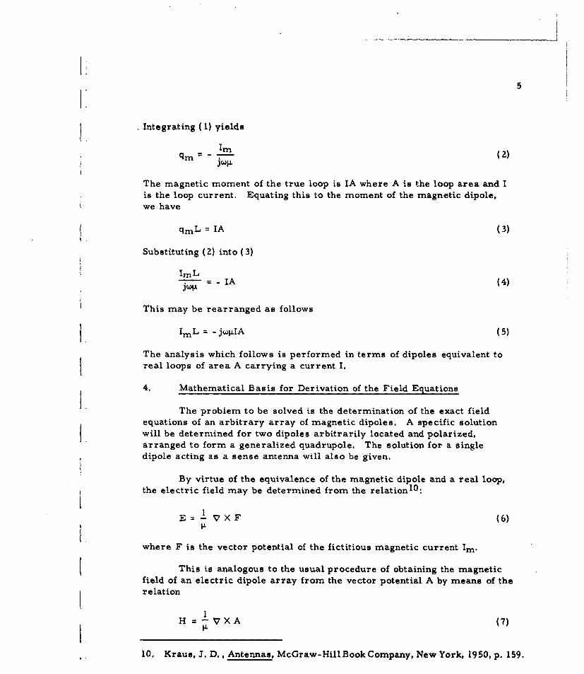
Integrating (1) yields

qm = -(2)

The magnetic moment of the true loop is IA where A is the loop area and Iis the loop current. Equating this to the moment of the magnetic dipole,we have

qmL = IA (3)

Substituting (2) into (3)

ImL--- -IA (4)

This may be rearranged as follows

SImL = - jwIA (5)

The analysis which follows is performed in terms of dipoles equivalent toreal loops of area A carrying a current I.

4. Mathematical Basis for Derivation of the Field Equations

The problem to be solved is the determination of the exact fieldequations of an arbitrary array of magnetic dipoles. A specific solutionwill be determined for two dipoles arbitrarily located and polarized,arranged to form a generalized quadrupole. The solution for a singledipole acting as a sense antenna will also be given.

By virtue of the equivalence of the magnetic dipole and a real loop,the electric field may be determined from the relationl 0 :

E VXF (6)

where F is the vector potential of the fictitious magnetic current Im.

This is analogous to the usual procedure of obtaining the magneticfield of an electric dipole array from the vector potential A by means of therelation

1

H =- VXA (7)

10. Kraus, J. D., Antennas, McGraw-HillBook Company, New York, 1950, p. 159.

IiIn the present case, for sinusoidal time varying fields, the magnetic

components may be determined from the relation

H=j V X (8)

By analogy to A, F is given by

F m dT (9)

For the dipole at Pk of Figure Z, equation (9) may be written as

k 47 rk'rkL. Fk = -•- f ImeJdAt-r c' / (10)

a

When the dipole is very short compared to rk, Im over the dipoleis constant, the dipole length is L, and hence equation (10) may bewritten as

Fk = 4(mLk ej (t ~ ) (I

If Fk is oriented in any arbitrary direction as shown, then the[. rectangular components of Fk are

Fkx = Fk sinekp cos ýkp

L Fky = Fk sin kp sin'Okp (12)

Fkz = Fk cos Okp

These are related to the spherical components as follows

SFkr = FkxsinO cosb + Fky sine sinO + Fkz cos 0

I FkO = Fkx cos 19 cos 4) + Fky cos 0 sin4b - Fkz sine (13)

FkO = - Fkx sin 0 + Fky cos

I:7

Substituting equations (12) into (13) and simplifying yields

Fkr = Fk[sine sinOkp cos('Okp - 4)) + cOs e cOs ekp]

Fke = Fk[IcOs 0 sinOkp cO(kp -( ) - sine cos ekp] (14)

FkO = Fk [sinekp sin('kp - 40)]

Reference to Figure 2 shows the dipole is located a distance rk fromthe point of observation where rk is given exactly by

rZ = r2 + rd 2 -Zrrd cOs If (15)

where

cos -= sine sin kcos(kt - 00k) + cos 0 cOs Ok

A binomial expansion of (15) yields

1 rd (rd2 - I- cosTy ..rk= r - cosY + T0 (1 (16)

When r >> rd the above is approximately equal to

Lrk = r cos7] (17)1 r 7

Substituting equation (17) into (11) yields

jW t r-rdcs-F i(ImL)ke c

iFrjk -I cos ] (18)r

A spaced loop will consist of two dipoles located colinear with theorigin and on the surface of a sphere of radius rd. This requires that

'1 + '2 = i (19)

Substituting equation (19) into (18) to obtain retarded potentials foreach dipole yields:

Fi( le W lIt (r - rdcos)]F1 1 rd

47r)e ( I r rcosy ) (20)

F? gImL) 2e

4Trr I + d cosB ']r

where

cos yl = sin9 sin0l cos(S -(4 ) + cos cos l (21)

An orientation which is convenient for interpretation of the fieldequations places the dipoles on either the x or y axis. This permits theE0 component to represent vertical polarization and the E0 component,horizontal polarization (although the effect of the earth has not been con-sidered in this analysis). Choosing the y axis requires that 01 = Sl = 90*and consequently

cosy-i = sin0 sins (22)

Rearranging equations (20) to have a common denominator andneglecting terms (rd/r)Z and higher order we have

Si[t ( r - rd sin! sin±)] +1- - rrji(i L)le c [I + --r sin 0 sin s

(23)

F m e [- (r + rd sin0 sinS)1 [ rs ]L)2 -W [ C A-rd sin 0 sins4

F2 247r

(24)

The retarded potential of the quadrupole mode is

F1 - F 2 i(ImL)e J C~) 32 rd sinOsin [ +5';r Nlr +-(jp-)Zl(25)

9

where (ImL)I = (ImL)2 and the dipoles are arranged to be parallel. Paralleldipoles require that

elp + 02p =T(26)

4 2'p = 4 'p + TT

Equations (14) then become

Fr = F - F 2 ] [sine sinelpcos(#lp - 4) + cosO cosolp]

Fe = [F1 - F 2 ] [cos0 sinOlpcos(#ip - 4) - sine cosilp] (27)

FO = iF 1 - F 2] [sin01psin(#1p - 4')]

5. The Electric Field Components for the General Spaced Loop

Equations (27) may be substituted into :equation (6) to obtain theelectric field equations. Expanding equation (6) yields

1 j =.1.(sin0FO) - -FJ] I sine orsinO -00, r sine---

+ cos e F, - ] (28)

ýi1 =l BF Fr OF29)1 Or 4,1= -5-0- r- FO]I 29Eor ion 80 ar r no0

= r Er (rF0) - -a-e =r -+ Fr -J (30)

The six required derivatives are

t ~t0 L), -P Zrn ) + sin4, sinzesin01pcos(4lip-4)+

+ cos20cos0lp] (31)

aFr J4I mL)Lprde (C) + sin 0 sin 0 sin0lp cos(,ip - 2.0) t

,Znr [(00r) (jfI-r) 2 J L

+ cos 0 cos 01ip cos (32)

10

jwa t r + 2FO - j(ImL)lp 3 rde = sin 9sini -+ 2-+ X

8r 2w jor (jor)Z 2 jpr) 3

X [cos e sin e lp cos(dil -p ) - sin 0 cos 0i p] (33)

We - I4ImL)l 2 rde ( .) __+ sine0 cos0sin0 1pcos(0-lp -2)

2w [or(jp'r)Z] P

- sine cos e Ip Cos ] (34)

aFo j L(ImL)lp 3 rde 1+ + 2 Xa-- r +T [TOr (jor) I 2 o

X sinl sinl8Ipsinosin(cpl- •) (35)

j.• t-.f

-e = (ImL)pZrde(C) + cos 0 sinO1 p sin 4sin(0 - 0)

3 2 I jr (jpr)Z I ( 36- (36)

Substituting these derivitives and equations (25) and (27) intoequations (28) thru (30) yields the electric field equations

Er~ ~~~j t -J l jr)3(~

- cos @ sin0 Ipcos •ip] (37)

(ImL) p3rde fr' 1

Er -J Zn + sine sinOlp X

X [cosc0 sin 19 + cos + cos cos37) +

+ [T.]sin 0 sin 0 lp sin• sin( lp - €)} (38)

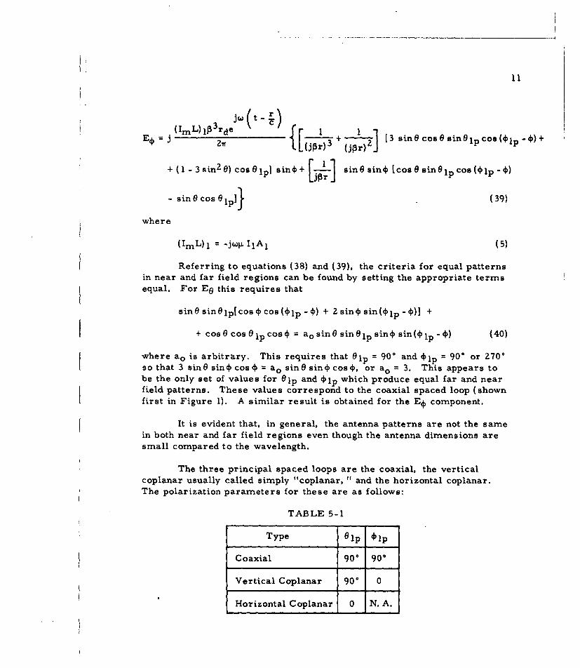
(ImL)lf33 rde (ZEý j 2 + [3 sin6 cos6 sinilp cos(Olp - )+

+ (1 -3sin2) cos9lp] sin+-I- 7 sin0sin [cosesinlp cos(0lp -)

- sin e cos e lp]} (39)

where

(ImL) 1 = -j(li I 1 A1 (5)

Referring to equations (38) and (39), the criteria for equal patternsin near and far field regions can be found by setting the appropriate termsequal. For Ee this requires that

sine sin9lp[cose cos(Olp -0) + 2sin4 sin(Olp-0)j +

+ cos cos lpcosý = aosin sin1p sin sin(-Olp-,) (40)

where ao is arbitrary. This requires that O1p = 90° and 4lp = 90° or 270°so that 3 sine sino cosO = ao sine sinO cosO, or ao = 3. This appears tobe the only set of values for Olp and 4lp which produce equal far and nearfield patterns. These values correspond to the coaxial spaced loop (shownfirst in Figure 1). A similar result is obtained for the EO component.

It is evident that, in general, the antenna patterns are not the samein both near and far field regions even though the antenna dimensions aresmall compared to the wavelength.

The three principal spaced loops are the coaxial, the verticalcoplanar usually called simply "coplanar, " and the horizontal coplanar.The polarization parameters for these are as follows-

TABLE 5-1

Type 6 lp Olp

Coaxial 900 900

Vertical Coplanar 90° 0

Horizontal Coplanar 0 N.A.

12

Substitution of these values and equation (5) into (37), (38) and (39)yields the following:

a. The Coaxial Spaced Loop

Er =0 (41)

E =- IPArdw4e c+ 3 + 1sin 9sin 2oo

0 4Tr 1 (jpr)3 (j pr) 2 j- r1 42(42)

Ip3Ard w4Le3 t 3e 3 + _i sin2 0sin 2 ý

4 1 T = 4( j pr ) 3 ( j p r ) 2 j- r n ( 4 3 )

b. The Vertical Coplanar Spaced Loop

Er Ip 3Ardwe (t ) [ -- L-o1 0 (44)

ZI T rw-r(t-)

E = - Zrr +jp)C (cos 241 - sin2 4O)__r) +1 ()pr

inr I sin(

I•p3Ard oýe c 3r? + 3 + I

8E r + T sin Z0 sin Z283 (jr)2

(46)

c. The Horizontal Coplanar Spaced Loop

ip ~ j AriIe(t -EE3Ard'je c + _ ] sin 0 cos 40 (47)21r =j " 3 (jpr} 2

13

Ee Ip3Ard Le' C 2 + ( Cos6) coso (48)

Ip 3 Arde 1 1

s W (cos20- sinZ0)

I ssin$ (49)

The above relations show that two special cases produce E fieldpatterns which differ for near and far field sources. These are: (1) azimuthor $ plane patterns for the vertical coplanar spaced loop for vertical polari-zation, and (2) elevation or 9 plane patterns for the horizontal coplanarspaced loop for horizontal polarization.

All other E field patterns for the above three special casesmaintain a constant shape for sources at any distance which is large com-pared to the spaced loop dimensions. It is to be emphasized that the caseswhere the patterns differ with source distance do not result from a parallaxeffect. The pattern shape changes due to parallax have not been calculated(they have been assumed to be negligible).

6. The Magnetic Field Components for the General Spaced Loop

As described in section 4 the magnetic field equations are easilyobtained from Curl E by equation (8). Expanding equation (8) yields

SHr (50) in 8

H r = in (sin0E,) - (50)Eir sinG Er 10 I(r)]

He =- 1 a (rZo) (51)

t.H = a--i (rEO) - al (52)0 wcLr a1r_ Be

These may be rewritten as follows

H r:j -- OrEO EO cos 0 aE0 (53wIr86 sin 0 sin 988

14

He 8~Er EO 8E 4 j(4wA[r sine 0 8 r (54)

*_= LrOEeEe BEr 155W~i L-ar r e r8

The six derivatives required are as follows

jW& t -

ar (ImL)p33 rde - (co 1 1

+sin 0sin 0 p cos 0 lp) (56)

BEr (ImL)p3rde(C) ___ 1

+w [3- + I sine0 cos 0 lp sink (57)

8E6 ~ ~ Zi (ImLP 47 ) 3~-~~ __ (jpr) 3 (pr2

3Eg (ImL)p~rde 1 3 + +

-ar-21r j[11(jpr)4 (jpr)2 J r-?]

X [sin~sin~lp~cs1Oc(4Olp-4-cO) sincoslin~o-+ csecsel o

+ L 3 s1nesine -lsioi(Op0 (59)

j Wa t - ) __

aEO (IML)p4 rde ' I__ + I 18r21 {[(jpr)3 (jr 3P 7jr)]X 3[3iO sinOspsinics(4)lp- 2) + (1-O 3o~sinZ)osi] + i~

+ [2 .+-.1- sin~siný[cos~sin~lpcos(40ip-4o)-sin~cos~lp}1(j~r)2 jpr 1J1

(60)

V 14

He-L 8Er. Eý 8E.$l(4

FOEO Ee 8 Er11~L -+T r8 - (55)

The six derivatives required are as follows

a ~jr J~(t -3r (ImL)p3rde Lur 1 1 (os coselp cos o +(jp3+ r-)2 J

+ sin 0 sin 0 p cos 4i p) (56)

Br j(ImL)f33rde ( C __ I 1 in1 o 1 9 eC lp sin4) (57)a427r [(jf3r)3 jp r-)2j

3Ee (ImL)f34 rde (c 3-8r - 2Tr (jpr (jpr) 3 + jpr) 2]

X [sine sineip~cosO cos((Op-0) + 2sin~sin(4ýlp-4)]I+cos~coseipcos 0]

+ [(j1 )+ 1r sine sineipsinlosin(olp-.)} (58)

a0 (ImLr) p-re (I~ ) ___ jr2

+ E ~r] in~sn61 si~t 1 - 24 (9

3 (IML)p~rde (t1

or 21, f(jpr)3 (jpr)3 (jr)

+ E+.Ll~sinelsin(4cose24) -c 1scos(. 1 ... )..sincos 1+

+ sinr) e~ siJ9I i( p-2)(9J7(60)

aEO (ImL)p3rd ( cBe {[(jplr)3 (jpr)21

X[3cos26sinlopcos (4p-O)-3-sin2Ocos~ip1sino+

+ E i- [cos 2esineip sinO cos(Olp -() -sin 20coseip sin.} (61)

Substituting these derivatives into (53), (54) and (55) with equations (38)and (39) yields

Hr I - 4 1rT J c tl jpr)4 (jpr)3 (jpr)2 II

+ Cos?-6) Cos (0lp -4) - 3 sin 20 cos 0 lp] + sine0ilpsin (0 i - 2.)]} (62)

He -I '4Arde ( c osepsn-

21T fl~pr)4 (jpr)3 I 6 1 L(jpr)4 (jpr) 3

+ - sino 3 sin 0cos 0sin e p cos (4)l- 4))+( 1 -3 sin~e) cos 0 l] +(j~3r) 2 j

+ ip1 sin 0sin60[ cos 0sinei p cos (.ip - )sin 0cos 0 p} (63)

H= -IA4 Arde - +Co (jr9] C5Cos 0lp Cos +

+2 2 +r n0si 9l+ sine sineipcosolp]+[ý;p )4 +(jpr)3+ (jpr)2J 1 n6S nip)

X Icos4~cos(4ilp - )+ zsin4)sin(ýPip- 0)J +cosbcosbipcosj)] +

+ jr Xsinb~sin~I9psin4~Bin(Otlp0)} (64)

Substituting appropriate values from Table 5-1 equations (62) through

(64) yield:

16

a. The Coaxial Spaced Loop

H -IAA3 rde3 c/ 3r 47rr) (jpr) 3

+ 1L 2(1- 3 sin29O sinZý) (65)

Ho IAP rdej C/ E 6 64w jr) (jpr)3

+ 3 + -L- sin 20 sin24 (66)(jp3r) 2 j3rl

- I p 4 r d j ( t ,H= 4w L (jpr)4 (jf~r) 3

+ 3Ž- + TF1- sin 1 sin2 (67)(jpr)2- jrIb. The Vertical Coplanar Spaced Loop

Hr =IP4Arde3 (tf - 3. E -+ JA sin2 0O sinZ24H 4 (jPr) 4 (3r) 3 (J~lr) 2

68

He = -Ip 4 Arde jw c E- r + 68ir [T7 r)4 (jpr)3

+ 3 + -!-1 sin 20 sin 20 (69)(jpr)2 - jPrj

17

I iHO Ip4Arde3 c 3 3 Co r0 2W`

'V 2W I..Ljp~r) (jpr)JL 1 ](coo2 - sin2 )

[-jP°r)2r j r70)

c. The Horizontal Coplanar Spaced Loop

j(71)ip4ArdeJ C)t- r)1

Hr 4+ -+ 3sin 20 sin4(jr) 4 3 (jpr)i

-i---- ~sin~(72)H If_4ArdeWL 3 + 3o Cos O

+ (cO o 0 - s inz 0)- 1'r s sin 4) (72)

Zi (j~r)4 (jpr)3 (jpr) - (73)

These equations also show near to far field differences for the same caseswhere differences were found with the electric field equations. These dif-ferences were listed at the end of Section 5.

7. The Electric Field Components for the Simple Loop SenseAntenna

A sense dipole located at the center of the spaced loop will havethe vector potential given by equation (10) or equation (11) with the addedcondition that rk = r. Therefore, by substitution into equations (14), thecomponents of F for the sense dipole are.

Fr = F[ sine sinep cos(p -( ) + cos0 Cos OPI (74)

i- I

18

Fe = F( cose sinOpcos(Op - ,) - sine cosep] (75)

Fý = F[ sineOp sin(Op - 0)1 (76)

where

F - 4w ( (77)

The six required derivatives are:

rae r *P(mL) 3e4w [j- cose sinOpcos(ýp-,) -sine cospi(78)

jW (t -r8 Fr jP(ImL)3 e -4[-L1 [sin 0 sin Op sin (Op -) (79)

Or-- 4?r + jp l

X [cosO sinepcos((ýp- d) - sin0 cosip] (80)

joe t- r)8F6 jIýLP(IML)3e (1! •F0 =J•(I L)34w1 j- ] cos 0sin 0psin(ýp -0)] (81)

I(ImL)3 e (r 4 + -I sine sin(op-o) (82)4wf L= jprj

8r (jJr)72

8- o (83)Be=

Substituting equations (78) through (83) and equations (75) and(76) into equations (28) through (30) yields the electric field equations forthe sense dipole:

UI

19

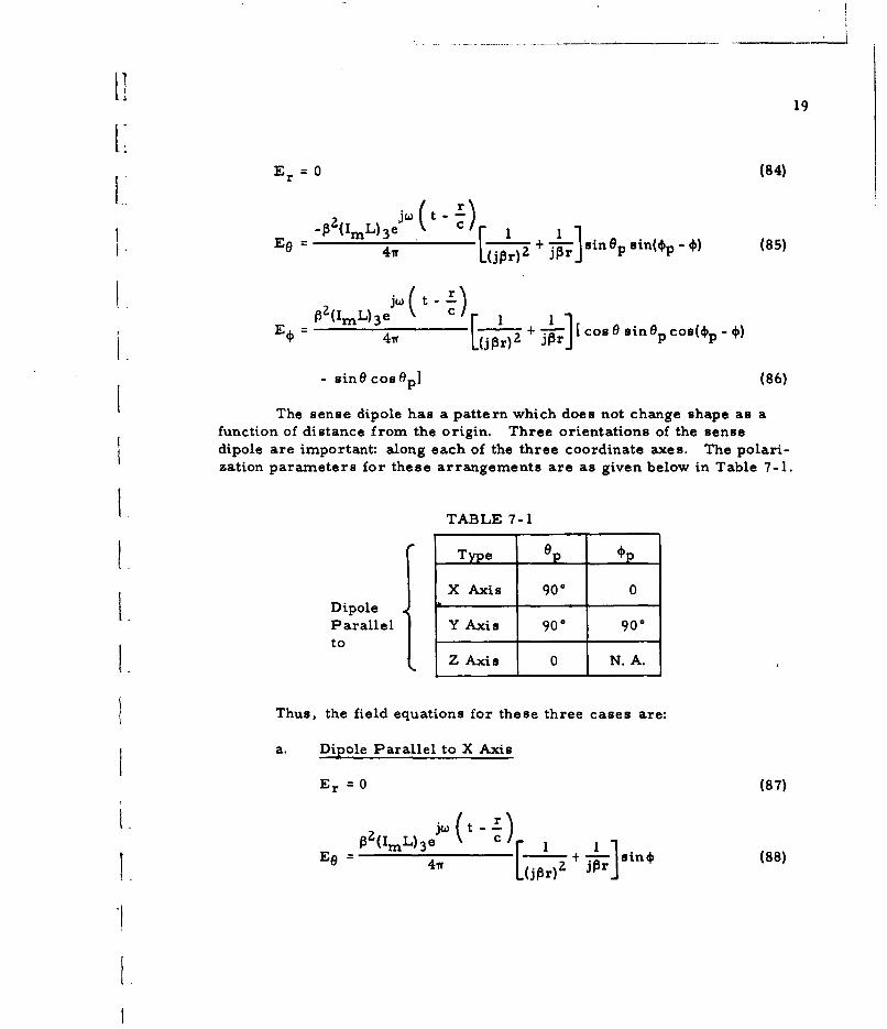
Er=0 (84)

LjfW) t rJ P(5S= P(ImL)3 e( + ] Co.ep sin O p - p) (85)

4 ir - I jfOr 2 j~rIE P Z(I mL) 3e

l E =4-r + j-• [cos 0 sin Op coS(Op - )

- sin0 coo ep] (86)

The sense dipole has a pattern which does not change shape as afunction of distance from the origin. Three orientations of the sensedipole are important: along each of the three coordinate axes. The polari-zation parameters for these arrangements are as given below in Table 7-1.

TABLE 7-1

Type p Op

X Axi s 90g 01.DipolegogoParallel Y Axis 90@ 90to

Z Axis 0 N.A.

Thus, the field equations for these three cases are:

a. Dipole Parallel to X Axis

Er = 0 (87)

132(ImL) 3 e (t -

E 6 = 4P 2(L3,I + -Ilsino (88)4.

[I

20

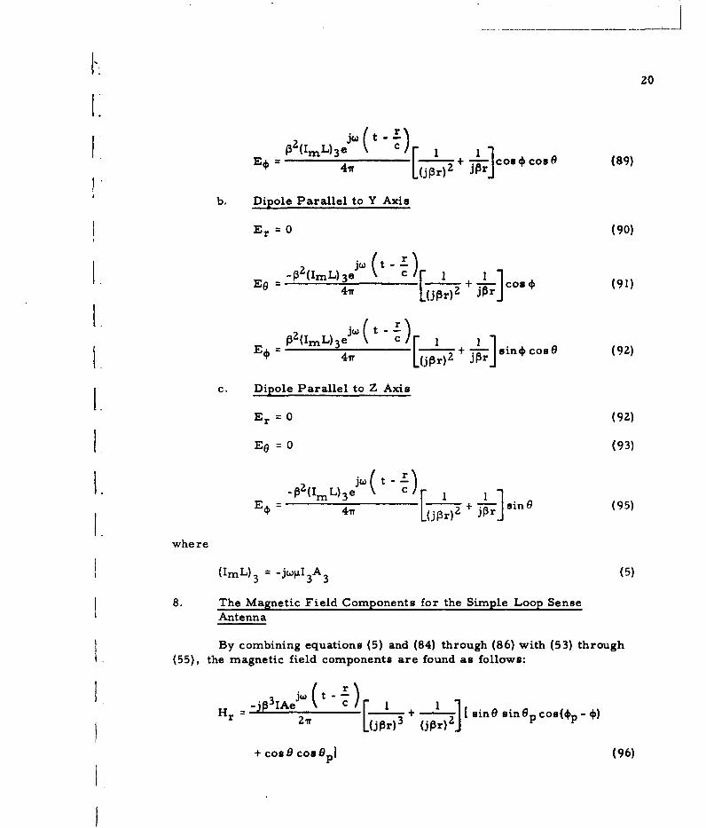
P2 ii L)3e~( t- 1 11

E[ = 4 + cos couo (89)'4v (r 7

b. Dipole Parallel to Y Axis

Er = 0 (90)

t

E := -p2(ImL) 3 e c + -1 - coo # (91)4(jp+)JPrJ

I. 2( , mL)3ejW( - r ) I ]-sin# cosO (92)

c. Dipole Parallel to Z Axis

Er = 0 (92)

EeO = 0 (93)

] _•~Z(ImL)3eJ'<t~r 1

E¢ = 41T [(jIML2 + -L sin0 (95)

whe re

(ImL) 3 -jW[I 3 A 3 (5)

8. The Magnetic Field Components for the Simple Loop SenseAntenna

By combining equations (5) and (84) through (86) with (53) through(55), the magnetic field components are found as follows:

Hr -) + Ir]' sin e sin OP cos(P - *)27 co= B o (96)

+ Cosa Cosa p] (96)

21

H6 +jp3jAe (~ I~4H9 =j41r (jr r) 2

+ CB [ cossinOp cosB (p - sinecosGp] (97)

H jp3iAeJw t - L 1 i

H = jp31A (j+r)2 I+J n sin(4Op-0) (98)

The field equations for each of the three orientations listed in Table

1. 7-1 are as follows:

a. Dipole Parallel to X Axis

jw(t.-)Hr - + I sine cos 0 (99)

Sjp3IA eJr(t- ) 1 1j ) z 1I

H19 A +j-r )+ I+ ----I cos Coss (100)4=r [Up r) 3 (j Pr) ' Tp-rI

-- _ + sink (101)41rf~r) 3 (jPr)2 TPT)

b. Dipole Parallel to Y Axis

Hr - F + sinO sin, (102)

He = 4p j t--r + I r)+ --L- cos~sinO (103)

41T (jt-r)3 (jPr)- J r

j0-3IAe-( ( . ]Hoj 4r7- cosin (104)

4w_________+ 1 1

c. Dipole Parallel to Z Axis

Hr 3j 1ejW - 7 + 1 I coo 4 (105)

-jp33IAe3O) i 1

IHO - 4 +-- +- sing (106)41r3r) 3 (j~r)2 jZr

Ho 0 (107)

9. Summary Tables of the Field Equations

The following tables are presented for quick reference and ease ofcomparison. Plots of the various field patterns are given at the end of thissection.

The first four tables refer to the spaced loop with the dipoles (loops)located at points on the y axis (y = rd, y = -rd). Tables 9i.5 through 9. 8 referto a simple loop oriented as indicated and located at the origin as would bethe case for a sense loop antenna. Table 9. 9 refers to a short electric dipolelocated at the origin and parallel to the z axis as would be the case for anomnidirectional sense antenna of the type for vertical polarization. Table 9. 9is provided from Kraus'- and is for the purpose of comparison to the otherantennas since this type sense antenna is frequently used with simple loopD/F antennas. In all tables the equations are regrouped according to polari-zation of the field.

Table 9. 1 Field equations for the general spaced loop antenna.

Table 9. 2 Field equations for the coaxial spaced loop antenna.

Table 9.3 Field equations for the vertical coplanar spaced loop antenna.

Table 9.4 Field equations for the horizontal coplanar spaced loop.

Table 9. 5 Field equations for the arbitrarily oriented simple loop antenna.

Table 9.6 Field equations for the simple loop antenna with axis alongthe X axis.

Table 9.7 Field equations for the simple loop antenna with axis along- the Y axis.

Table 9.8 Field equations for the simple loop antenna with axis alongthe Z axis.

Table 9.9 Field equations for the short electric dipole sense antennaalong the Z axis.

4�<3>

4-� 3, -. - - - _ ___ 3-

liii 23

Iii p 1 ! I

S�flIiIi 1

V iI

S

1Ii I

2-�

- � I

V Ii�

Li ,�' i -jj -

IIV -

U 1 � -RA .� I :* SI3 * S�7 I. II I

S - * '� :L I '* * 4 p.

* I � Ip. *

2

V I � Ii�L 1 4 �A. I

1% � * f-, -

V I -r� � 7�U

11111 c.-. kill I SlIP - I- I I I

*i� I kill- - -

A%. I.*� I� I�j I�I I�I

5 5 p 5 5 5

U I?U ___________W@IW')�I4 115U*SA U*�IJItd W��U

I Li

4~24

TASSAI9.3. FULD MOVATIONU PMa 21 COAXIAL $PAC=, LWoe

14l 4. 71 __ (43)

UTABLE 9.3. FIE2LD EQUATION FOR THE VERTICAL COPLANAR SPACED LOOP

.00 0 (44)

H, -.4. 7p,-)3 3 3 .01 .2 "

llid

(J#, +L+-1. .1. 1@L.i(6

TABLE9-4. FIELD EOUATIOU TOR THE HORIZONTAL COPLANAR SPACED LOOP

1c, . 14r---- N (150-1- IS-p-)

(Sp. ) I.) coo#) (75)

~IP (J- 0 ) + itl est 14 (49)

me

-+

i t f

L"O _lm"P t-R" t"*AGIMPI

Some of the pattern variations which correspond to various condi-tions on the general field equations (38) and (39) for the general spacedloop are plotted in Figure 3. The patterns have been grouped to showpattern shape changes as a function of dipole orientation or type of spacedloop. Patterns at the extreme left therefore correspond to the verticalcoplanar spaced loop and patterns at the extreme right correspond to thecoaxial spaced loop. The patterns show variation with distance to thesource in the vertical direction; those at the top correspond to the nearfield and those at the bottom to the far field. The patterns are also groupedLi according to polarization.

Starting with the coaxial spaced loop, (on the right in Fig. 3) asthe dipoles are rotated so as to approach the configuration of the coplanarspaced loop two of the four lobes decrease in amplitude and two of thelobes increase. This effect occurs for both near and far field sources.However, for sources in the intermediate range (in the vicinity of one-third wavelength) the nulls are replaced by minima. These minima are ingeneral not 900 apart.

It is evident that as the transition is made from the coaxial to thecoplanar spaced loop four nulls are maintained if the source is in the nearfieldbut the four nulls reduce to two if the source is in the far field.Polarities are not shown in Figure 3, however, the four lobes of thecoaxial spaced loop pattern have alternating polarities while the two lobesof the coplanar spaced loop have the same polarity. This transition isevident in the far field patterns of Figure 3 for both vertical and horizontal

LIpolarization.

The patterns for horizontal polarization do not exhibit changes inshape due to distance to the source as in the case of vertical polarization.I Therefore, the last row of patterns in Figure 3 applies to any sourcedistance which is at least greater than the spacing between loops.

The similiarity between the two patterns corresponding to ýlp= 90°,

*Ip = 67-1/z* for vertical polarization indicates that the modification tothe pure coaxial spaced loop pattern, which is produced by a slight changein the angle l, is very similar to the distortion due to an omnidirectionalcomponent. This is interesting in that in the past similarly appearingdistorted spaced loop patterns have been experimentally obtained whichdid not seem to be related to vertical pickup in the antenna system.

[I

Ii

27

low

r- IOOX

PbOMR 3.AZIMUTH PLANE PATTEINS FOR THE SPACED LOOP.

Glpuw" 4MIP VOUIWJ

28

10. Combinations of Spaced Loop aud Simple Loop Antennas

An arrangement of three loops in certain cases produces patternswhich are symmetrical about only one axis and hence may be used as D/Fantennas without sense ambiguity. The three-loop antenna developed undercontract NObsr-64585 is an example and corresponds to combining theequations from Table 9-2 with-those from Table 9-6. Details of the phasingand amplitude difference problems which arise in this case were reportedin the final report of the same contract 1.

For vertical polarization the total response will be the sum of theE& components; for horizontal polarization it will be the sum of the E+components. Considering only the response to vertical polarization, if thespaced loop and simple loop outputs are simply addedthe voltage presentedto the receiver will be the sum of equations (42). (see Table 9-2), and (88),(see Table 9-6). This correspbnds to the three-loop configuration wherethe simple loop axis is perpendicular to the coaxial spaced loop axis.

For this case there are two inverse distance terms in the simpleI) loop response equation and three inverse distance terms in the spaced loop

response equation. This difference produces both an amplitude and aphase change in the total response as a target source is moved from thefar to the near field. Since all target sources are located in the far field(that is, they are at least many wavelengths away) while local reradiatorssuch as are found on board ship are generally in the near field, it is evidentthat the complete response must be considered.

Examination of the equations in Table 9-1 shows that the nearfield E or H terms are all in phase, that is, the electric field of the simpleloop is in phase with the electric field of the spaced loop when the sourceis near by. This means that when the three-loop antenna is tested with anearby source, such as the transmission line method in a screen room,the outputs may be simply added with zero phase shift. On the other handthe equations show that when the source is in the far field, the response ofthe simple loop is in quadrature with the response of the spaced loop anda 90-degree phase shift is required to combine outputs to produce a properD/F pattern. For sources at intermediate distances, the phase differencevaries between 0 and 90 degrees. It is effectively 90 degrees for all distancesgreater than three wavelengths and effectively zero for all distances lessthan 6 X 10-2 wavelengths. It is approximately 45 degrees at one-third ofa wavelength.

11. Travers, Douglas N., et al., "Methods for the Reduction of Reradiation

Errors in Naval High Frequency Shipboard Direction Finding, " FinalDevelopment Report, Southwest Research Institute, 1 January 1961.

29

L IIf the spaced loop is used alone without a simple loop, equations (42)

and (67) (vertical polarization, coaxial spaced loop) show that the shape isindependent of the distance to the source. Experimental evidence has shown

that even when the sources are very close such that the distance is equalto the spacing between loops the shape of the pattern is modified onlyslightly. The general shape in this case remains the same, that is, fournulls are obtained 90 degrees apart.

Another point evident from the equations is that the near field termsare independent of frequency. This means that if testing is conducted in ascreen room, the variation in gain required to mix the signals with equalamplitude (or to provide some degree of sense) will appear to be less than

that which is actually required when the target is distant. This effect willbe more noticeable if the operating frequency range is increased.

It is also evident that the simple loop far field is proportional to

frequency while the spaced loop far field is proportional to frequency squared.ii The relationship is such that for similar sized small antennas the far fieldof the spaced loop is much less than that of the simple loop at low frequencies.

U (This point is considered in mere detail in sections 15 and 17 on signal-to-noise ratio). This requires that the isolation between circuits of the twoantennas be relatively high prior to combining.

Another particularly important point is that the geometry of the

coaxial spaced loop will not be critical for a source in the near field butwill be so for a source in the far field. The reason for this is explained inthe final report of contract NObsr-64585, in terms of the field equations,however, it is related to the fact that the output for the far field source

results from a field phase difference across the array whereas for nearbysources the output results from amplitude change across the array. It isthus necessary when constructing spaced loops where construction tolerances

are in doubt, to evaluate pattern quality with a far field source. It is quitepossible to experimentally obtain near field spaced loop patterns which areapparently perfect, from an antenna which when tested in the far field,

t produces so much distortion that only a dipole mode can be observed.

Another combination of three loops which will produce a pattern

with one axis of symmetry is obtained by rotating the simple loop 90 degreesfrom the position considered in the last example. This produces threeparallel coaxial loops. The response may be studied by combining equations

(42) and (91) for the electric field and (67) and (104) for the magnetic field.There is little theoretical difference between this case and the one previously

considered.

U 30H

The third possible combination with the coaxial spaced loop wherethe simple loop axis is vertical is not important for cases where it is desiredto receive only vertical polarization. The horizontal loop does not respondto vertical polarization.

There are a number of combinations possible with the coplanarspaced loop. One of the most important of these is the combination of thevertical coplanar spaced loop and the simple loop aligned with its axisalong the X-axis. This arrangement results in three parallel loops alllying in the same plane. This antenna was first investigated by Friis priorto 192512.

The response of this combination may be investigated for verticalpolarization by combining equations (45) and (88) for the electric field andequations (70) and (101) for the magnetic field. Most of the comments madepreviously concerning the coaxial spaced loop are also appropriate for thiscombination with the exception of pattern shape as a function of distance tothe source. It is evident from equations (45) and (70) that the shape of thepattern undergoes a change as the source is moved from the far field to thenear field. This is in addition to the amplitude and phase changes. Further-more, the change is different for the E and H fields. The far field responseis proportional to sin2 $ as was-shown by Friis so that the pattern has two

V• nulls and two maximums, both maximums being of the same phase. In thenear field the electric component is proportional to (cos Zn - sin 2?) and themagnetic component is proportional to cos 2,, thus the response patternhas more than two nulls for sources in the near field.

An antenna of this type will not respond to local shipboard reradiatorsin the same manner that it responds to distant targets. It is also true thatif the antenna is phased with a simple loop, as was done by Friis, theresponse of the spaced loop will change according to equations (45) or (70)but the response of the simple toop will change according to equations (88)and (101). This occurs in such a way as to produce no change in the shapeof the loop pattern, but a change in the spaced loop will occur. Thus, thebasic assumption made by Friis that this combination can be used to producea null in the back direction of the forward lobe is only valid for far fieldsources. For instance, if such a combination is designed to produce a null

12. Friis, H. T., "A New Directional Receiving System, "Proc. IRE,Vol. 13, December 1925, pp. 685-707.

1;

U 31

in the backward direction on the basis of a far field analysis in ordea to.reject reradiation from a local source such as a reradiating mast, the nullwill not be produced and the antenna will respond to the mast.

I Other combinations of three loops may be arranged for either nullor max type direction finders for either vertical or horizontal polarization.In these instances it is possible to arrange the loops for response to onlyeither one polarization or the other but it does not appear to be possible tomake an arrangement which re.sponds equally to both polarizations. It ispossible, however, to have the antenna respond with a null to both verticaland horizontal polarization if only the spaced loop mode is used.

For instance the coaxial spaced loop has four nulls for verticalpolarization and two nulls for horizontal polarization. These combine insuch a manner that it has two nulls which remain fixed for any polarization.Similarly in the far field the vertical coplanar spaced loop has two nullsfor vertical polarization and four nulls for horizontal polarization such thattwo nulls are always maintained for any polarization. When used in com-bination with simple loops, however, these advantages are lost because thesimple loop has two nulls for vertical polarization and two nulls forhorizontal polarization; however, they do not concide [see equations (88)and (89)].

11. Effective Height of the Spaced Loop

Ii The effective height or effective length1 3 of an antenna is a quantityused to indicate the effectiveness of the antenna as a radiator or as a collectorof electromagnetic energy in a certain direction. The term is often used inconnection with electrically small receiving antennas such as loops and assuch is often defined as the constant of proportionality between inducedL: voltage V and incident field intensity E

V = heE (114)

- The effective height may also be derived fr,-m consideration of theantenna as a transmitting source. In this case the effective height is the

Li length of an equivalent linear antenna with uniform current distributionwhich radiates the same field as the antenna in question, in the directionperpendicular to its length. Both transmitting and receiving effectiveheights are equal,and the quantity is independent of antenna losses or couplingnetworks to the receiver.

13. The term effective height is meant in the original sense as in equation(114) and is not to be confused with the height of the antenna above ground.

The radiated far region field of a current element of lenigth di

I jin a direction perpendicular to its length is given by the far field term ofequation (I110) F4. Neglecting phase this field is.

E I 1.p-3 - (115)

4wcEpr 4irwc 2~r 4wec Zr

Therefore, the field intensity produced by an antenna having aneffective height he will be

Li IMewLiE= (116)

Hwhere I is now the current at the terminals of the antenna and also theuniform current in the element.

Equation (116) may be solved for the effective height

he = 4¶ff CcrE (117)

This is equivalent to

he4,rE(18h=IWIL

From the field equations derived in the previous sections, theLieffective heights may now be derived by substitution into equation (118).

For instance, for vertical polarization (E&), substituting the far field termfrom equation (38) yields the effective height of the general spaced loop

he=-- 4w rwLsn&sin sin len(+ip -) (119)

and in free space

I heI = I Zp2Ard sin8 sin~ uin8 1p(sin~ljpcos+. cos~ 1l sin+)j

V (IZO)

For the coaxial spaced loop Olp =*1p= 90* and the effective height is

V het =IZPArd min 0sin+ cosl + IPZArdsine in2+ l Z

14. Jordan, E. C., Electromagnetic Waves and Radiating Systems NewYork, Prentice-Hall, Inc.,. 1950, p. 305.

V,

33

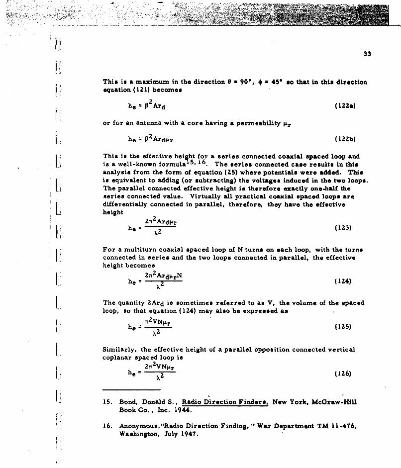
This is a maximum in the direction 0 m 90%, 450 so that in this directionequation (121) becomes

he = P2Ard (1ZZa)

or for an antenna with a core having a permeability Or

he = P2 Ard&Ir (lZ•b)

This is the effective height for a series connected coaxial spaced loop andis a well-known formula15. 16 The series connected case results in thisanalysis from the form of equation (25) where potentials were added. Thisis equivalent to adding (or subtracting) the voltages induced in the two loops.

H The parallel connected effective height is therefore exactly one-half theseries connected value. Virtually all practical coaxial spaced loops aredifferentially connected in parallel, therefore, they have the effectiveheight

ZWr2 ArdIrhe 2 (123)

For a multiturn coaxial spaced loop of N turns on each loop, with the turnsconnected in series and the two loops connected in parallel, the effectiveheight becomes

27r2 ArdLrNhe = X (124)

The quantity ZArd is sometimes referred to as V, the volume of the spacedloop, so that equation (124) may also be expressed as

Sa' 2 VNp~r

he - 7r 2V-__ 125)X2

Similarly, the effective height of a parallel opposition connected verticalcoplanar spaced loop isS2Zn 2VNi~r

h 2iVNL (126)

15. Bond, Donald S., Radio Direction Finders, New York, McGraw-HillBook Co., Inc. 1944.

16. Anonymous."Radio Direction Finding, " War Department TM 11-476,Washington, July 1947.

L34

The effective height of a horizontal coplanar spaced loop is zero for verticalIi polarization; however, for the E+ component (representing horizontal

polarization) the effective height is the smre as the vertical coplanar spacedloop for vertical polarization, or equal to equation (126). The factor j&r

in the above equations may be taken as the effective permeability of a core(for instance ferrite) inserted through the loops of the antenna (pair -).

12. Radiation Resistance of the Spaced Loop

The importance of the radiation resistance lies in the fact that itH may be used to determine gain and the signal-to-noise ratio if the effective

height is known. It is also instructive in illustrating the difficulty ofimpedance matching the small spaced loop antenna for maximum powertransfer.

The radiation resistance of the spaced loop antenna may be easilyfound by the Poynting Vector Method of integration over a large sphere.The radiation resistance is given by the ratio of the power flowing throughthe sphere to the square of the RMS terminal current of the antenna. Thus

w2L ffHzds(Rr 1 2 (127)

rme rms

where ds is the area increment on the surface of the sphere, and H is thecomplete magnetic field of the antenna in the far region. Since the radial

(A magnetic field is zero in the far region, H is given by

HH + '61 + -41' H&tI ,HO (128)

Therefore

SH 1H012+ IH.1 (129)

or

H'= IH01 -+ IH,1 2 (130)

Substituting equation (130) into equation (127) yields for free space

f• f (HI2+IHl7)d

r Z5Rr= (131)S212rm s

35

The far field terms, H& and H+i, are obtained from equationzs (63) and (64)Ii~p .4rdjw t . r

H9 AIrdet C cos 0 sin 0 p cos(+ ip - 40)

- sin0cos0lpJ sinisin& (132)

-IH AIrde ( ) [ sinu sin ipsin, sin(+ip - 'iJ (133)

Squaring and adding yields

4 _2(_r)_[ sin>2. sinZO(cos 2 0 sin20ipcos2 (•Ip- ? )

+ sin2 9 cos 2 e1p _ Zsin O cos 8 sin Olp coso 1pcOS•p1p

'II + sin 2 Oipsin 2 (ýip - +4)M (134)

The area increment is

ds = r 2 sin( d~dý (135)

I! Therefore, equation (131) becomes!! ,<,. =,-. rp3,<,l f2wfRr 2 C [ .d] f f sin2z sin3 0jcos 2 e sin 2 O1pcos 2 (*1p- *)

0o L2- msJ 0 0

+ sin2 & cos 2 Olp - sin2O sin lpcos 01p coS(4ip -l

+ sin 2 01p sin2 (•1p - 0)4] ddMO (136)

The integration is straightforward and results in the term 8w(2.-ii sin2Olpsin2 jip)/15. Therefore, the radiation resistance of the series

connected general spaced loop is

2

Rr I/ L-ZIrnsI L- (2 - sin2 Olpsin?*1p) ohms (137)0 w{ms 1

36

This is equivalent to

SRr 9.8 asX( d5 (2 - sin2Olpsin2*1p) ohms (138)

I i For parallel connected loops the radiation resistance will be one-fourththe series connected value. For the coaxial spaced loop, Olp = 90", *lp= 90",L and the radiation resistance becomes

Rr = 9.85 X 10 s )2 ohms (series connected)Ar2 (139)

Rr = 2.46 X 105 (--A ohms (parallel connected)

41(140)For the coplanar spaced loop (either vertical or horizontal) the radiationresistance is

Rr = 1.969 X 106 (-31 ohms (series connected)z (141)

SRr = 4.92 X 105 ( 2 ohms (parallel connected)X

(142)

These values are exactly twice the values for the coaxial spaced loop.

The radiation resistance for the spaced loop varies as the inversesixth power of the wavelength. Thus even though the constant coefficientappears to be large, the radiation resistance is quite small for Ard << X3.In Figure 4 the radiation resistance of two spaced loops of typical sizeis plotted versus frequency. It is evident that impedance matching of theradiation resistance to the receiver input is not possible by any ordinarymeans. It is further evident that the radiation resistance is negligible withrespect to loss resistance for ordinary conditions, and typical wire sizes.

13. Gain of the Spaced Loop

The gain of an antenna is related to the effective height and radiationresistance by the equation 17

120w 2 (he) 2

g~ (143)

17. Jordan, Edward C., Electromagnetic Waves and Radiating SystemsNew York, Prentice-Hall, Inc., 1950, p. 417.

137

1. ~APPROXIMATE LOS RESISTANCE OF TENMETERS OF .1 IN. 01A. COPPER WIREAORDINARY TEMP RT EA

RADIATION RESISTANCE SERIES.CONNECTED COPLANAR SPACED

-LOOP. L

S -RAIAIONGELO RSTANCE RADIATION RESISTANCE PARALLEL

SINGE LOP A.5m2 - -CONNECTED COAXIAL SPACED LOOP

54

65

rRADIATION RESISTANCE

FOR A TYPICAL HIGH

16- FREQUENCY SFACED LOOP(LOOP SPACING u 2 METERS)

(LOOP AREA x .5 METERS')

FREQUENCY (MCS)

__ ____ _ ___-I

38

Substituting equations (120) and (137) yields the gain of the general spacedloop for vertical polarization

15 sin 2 0 sin2 01p( sin2 Olp sin 2 2ý - 2 sin2ýlp sin2ý sin2o + 4cos2Olp sin440)8 T (2 - sin2 Olp sin 2 olp)

(144)

- For the coaxial spaced loop 0 1p= 90*, 4 lp= 90' and equation (144) becomes

S15"- sin 2 0 sin2 20 (145)

This is maximum at 0 = 90°, 45° hence in this direction the gain is

15 (146)8

For the coplanar spaced loop 0 lp = 90°, 'ip = 0 hence the gain for vertical

polarization is30"=" sin2 O sin4 ( (147)

s8 n

This is maximum at 9 = 90", 90* hence in this direction the gain is 1 8

15 (148)

The above values apply whether the loops are connected in series orPparallel.

14. Effective Area of the Spaced Loop

The effective area is another parameter for expressing the effective-ness of a receiving antenna. It is defined in terms of the gain of an antennaby the relation1 9

Ae = X-9 (149)41r

Using this relation it can be shown that the effective area is the ratioof power available in the antenna to the power per unit area of the appropriately

S18. In agreement with Shelkunoff, Antennas Theory and Practice, page 199,No. 6-1.6.

19. Jordan, Edward C., Electromagnetic Waves and Radiating Systems,N.Y., Prentice-Hall, Inc., 1950, p.416. Also Shelkunoff, S. , AntennasTheory and Practice, N.Y., John Wiley, p. 185.

39

polarized incident wave. That is, the received power is equal to the powerflow through an area equal to the effective area of the antenna. Substitutingequation (143) into equation (149) yields

As = 30nhe (150)SRr

or for vertical polarization

Ae 5-- square meters for the icssless3. 27r coaxial spaced loop (151)

A =1 square meters for the losslesscoplanar spaced loop (152)

The above relations hold for either series or parallel connected loops. TheI. power received is therefore

Pr = PAe (153)

V where P = power in an incident wave E in watts per square meter, orE2 E2

P E = -watts/m 2 (154)

IThe power available in the antenna is therefore

EzAe (Ehe) 2 =(Ehe62 1

P 120 -7 4R, " watts (155)

The power which is ordinarily delivered to the receiver is

in( ) = 1-_ watts (156)2i K in

where Rin is the equivalent receiver input resistance. Hence the efficiencyof the power transfer to the receiver is

Rr X10

eff. =-- X 100% (157)Rin

I From examination of Figure 4, it is evident that this efficiency must be inthe range of much less than 1 percent for most frequencies. This is simplyanother way of showing that,practically, the spaced loop is not an efficientantenna. However, for receiving applications, it is more important to con-sider the signal-to-noise ratio than maximum power transfer. This is coveredin the next section.

Li 40

15. Signal-to-Noise Ratio of the Spaced Loop Antenna

It is of interest to know the maximum signal-to-noise ratio obtainablewith the spaced loop and to determine the weakest field strength which canbe received in the ideal case and in the practical case. The material whichfollows is based on equations derived by Burgess 2 0 .

In computing the signal-to-noise ratio in receiving systems, it isnecessary to estimate the noise arising in the antenna. Thermal noise isgiven by Nyquist's theorem2 1 which states that the mean square fluctuatione. m. f. in the frequency band v to v + dv appearing in an impedance R + jX: 7Zis given by

de•- = 4kTRd v (158)

where k = Boltzmann's constant = 1. 374 X 10-23 joules per degree Kelvin,and T is the absolute temperature in degrees Kelvin. The value R isassumed to be constant over the bandwidth dv; if R is a function of frequency,a more general form of equation (158) is required22 . However, for thepresent analysis we will be concerned with bandwidths which are less thanone-half of one percent of the center frequency, so that while the previouslycalculated radiation resistances are rapidly changing with frequency, thechanges are small over the bandwidths considered and equation (158) isclosely approximated.

Burgess shows that the radiation resistance of an antenna canapparently be the source of thermal noise and that it obeys Nyquist's theoremwhen the aerial is in radiative equilibrium with its surroundings 2 3 . Thus

de-r 4 4kTRrd v (159)

20. Burgess, R. E., "Noise in Receiving Aerial Systems," Proceedings ofPhysical Society, Vol. 53, May 1941, p. 293.

21. Nyquist, H., "Thermal Agitation of Electric Charge in Conductors,Physical Review, Vol. 32, July 1928, p. 110.

22. For instance see Terman, F., "Radio Engineers Handbook, " p. 476.

23. Burgess points out that this statement is in disagreement with otherauthors in papers published prior to his 1941 paper. The validity ofBurgess' paper now seems well established however.

41

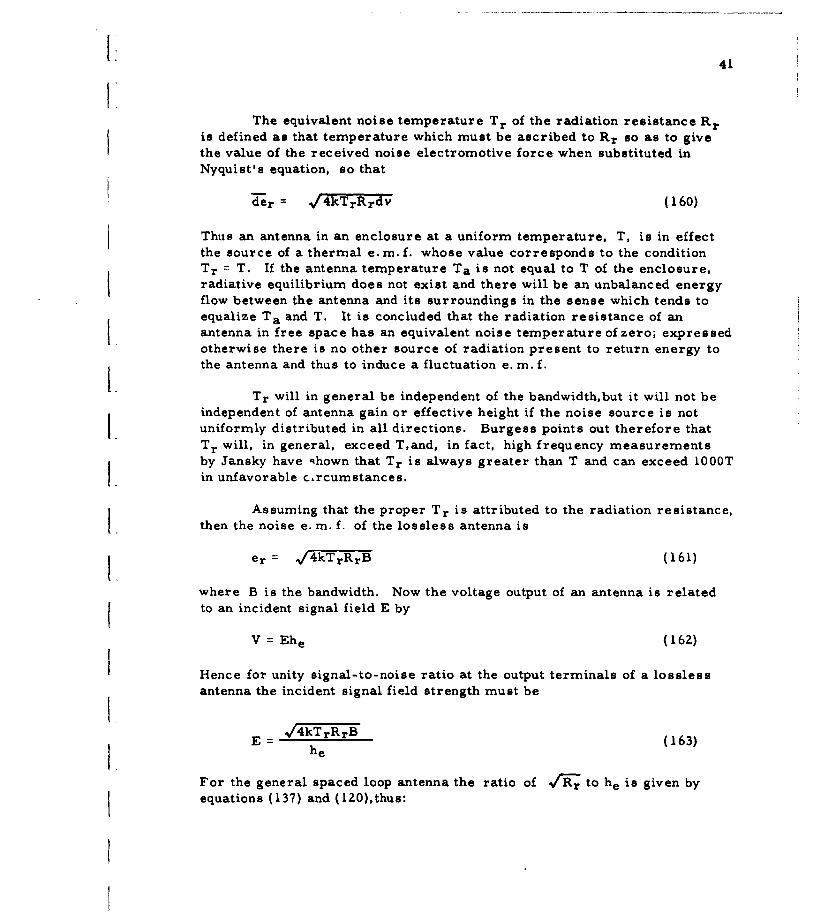
The equivalent noise temperature Tr of the radiation resistance Rris defined as that temperature which must be ascribed to Rr so as to givethe value of the received noise electromotive force when substituted inNyquist's equation, so that

der ./4kTrRrdv (160)

Thus an antenna in an enclosure at a uniform temperature, T, is in effectthe source of a thermal e. m. f. whose value corresponds to the conditionTr = T. If the antenna temperature Ta is not equal to T of the enclosure,radiative equilibrium does not exist and there will be an unbalanced energyflow between the antenna and its surroundings in the sense which tends toequalize Ta and T. It is concluded that the radiation resistance of anantenna in free space has an equivalent noise temperature of zero; expressedotherwise there is no other source of radiation present to return energy tothe antenna and thus to induce a fluctuation e. m. f.

Tr will in general be independent of the bandwidth,but it will not beindependent of antenna gain or effective height if the noise source is notuniformly distributed in all directions. Burgess points out therefore thatTr will, in general, exceed T,and, in fact, high frequency measurementsby Jansky have -hown that Tr is always greater than T and can exceed 100OTin unfavorable c,rcumstances.

Assuming that the proper Tr is attributed to the radiation resistance,then the noise e. m. f. of the lossless antenna is

wrer = /4kTrRrB (161)

where B is the bandwidth. Now the voltage output of an antenna is relatedto an incident signal field E by

V = Ehe (162)

Hence for unity signal-to-noise ratio at the output terminals of a lossless

antenna the incident signal field strength must be

E /4kTrRrB (163)he

For the general spaced loop antenna the ratio of /r to he is given byequations (137) and (IZO),thus:

42

he 2PZArd sin& sini sinOlp(sinIpcos4O - cosolpsinr1)

(164)

Note that the size of the spaced loop cancels out so that equation (164)simplifies to

_ 4w i/(z - sin2 0pSin2�4P)- series or (165)She k� sin0sin sinO'lpsin(40j -p ) parallel

Thus the weakest field which a lossless spaced loop antenna can receive is

1.4 4kTr B (Z- sinzblp sinz4 1P)E(o)min = T sin &sin blp sin0 sin(elp - 41) (166)

It is interesting to note that this field is independent of the size (Ard) of thespaced loop, therefore, it is apparent that the designers'desire to make thespaced loop large is to overcome effects due to noise in the associatedcricuits and the antenna loss resistance.

For the coaxial spaced loop (Olp = 9*p 90) equation (166) becomes

E 87 r 4-kTrB(17"(o)min = X sin 9 sin 246

The effective height is maximized in the directions 9 = 90%, 0 = 45° hence

E(o =in 167r 4kTrB = 8PqkTrB (168)E~)min. ...

The corresponding expression for the vertical coplanar spaced loop is

E(o)min = 8P sf 2kTrB (169)

For typical conditions of current interest assume

X = 100 meters (f = 3 mc)Tr = 290* KelvinB = 10 X 103 cycles

43

Then the theoretical minimum fields at 290°K (16. 8C) for either series orparallel connected spaced loops are

E(o)min = .00317 pLv/meter (coaxial) (170)

E(o)min = .00217 iv/meter (coplanar) (171)

Field strengths of these values will probably never be observed inpractice for at least three reasons, (1) the antenna will contain some lossresistance which will be a source of noise and, in general, the value of RrL for a spaced loop will be small compared to this loss, (2) the couplingcircuits and the first amplifier will be sources of noise which, in general,will be large compared to Rr noise, and (3) the value of Tr will often beabove the assumed value of T = 290°K because of noise sources in theenvironment of the antenna. It is the purpose of the remainder of thissection to estimate the degree to which these factors affect spaced loopsignal-to-noise ratio in practical cases.

Consider the general case of an antenna (in this case a spaced loop)coupled to an amplifier as shown in Figure 5.

- coupling firsL. V =Eh ,V=E network ---- ,amplifiez

FIGURE 5

The coupling network is linear and passive. It may contain resistances,tuned circuits, etc., including loss resistances. The first amplifier maybe any active network with sufficient gain and with an equivalent inputimpedance of Rin + jXin where Rin is a noise source.

The mean square noise e. m. f. at terminals 2-2 is given by

en 4kB [naTrRr + T (ZnR 1172)

where Rs is the resistive component of the sth impedance, element Zs ofthe network including loss resistance in the antenna but excluding radiation

44

resistance Rr of the antenna, ns = voltage transfer ratio from the impedanceZa to terminals 2-2, na = voltage transfer ratio from the antenna to terminals2-2, and T = temperature of the resistances in the coupling network.

Amplifier noise may be taken into account by adding a term 4kTBRvwhen Rv is the equivalent noise resistance of the amplifier input, thusequation (172) becomes

s 2 1 /2 (1 7 3)en = 2 q-V [naTrRr + ZnsRs + TRy] (173)

The signal-to-noise ratio is therefore the ratio of equation (162)to equation (173), hence

received signal V - Ehena

received noise Zn 2 5'0 [naTrRr + T

(174)

When the antenna is lossless, the coupling network is lossless andthe first amplifier is noise free, the absolute maximum value of the signal-to-noise ratio is obtained. This value is Po where

I . Ehe (175)0o 2 41 • Tr Rr (5

This signal-to-noise ratio is one to one at the field strengths mentionedpreviously. Substituting equation (175) into equation (174) yields the practicalsignal-to-noise ratio

P0P- P o"] / (176)1 T(YnsRs + Rv)1

I + TrRrna J

Substituting equation (175) into equation (176) and substituting thespaced loop~values for he and Rr, equations( I 20) and (139), yields the signal-to-noise ratio of the one-turn general spaced loop in free space

naEP2 Ard sin & sinio sin &1p sin(ýlp) -X3

'=IkB [Tr 9.85 X 105 (Ard)Z (2 - sin2 &lpsin2 lp) na + T(EnBZR + Rv)X 6 ]

(177a)

Note this is stated for series connected loops. When the loops are parallelconnected the signal-to-noise ratio will be:

45

naEP2 Ard sin & sin sin Olp sin(ýlp p-)3

2 •lB [Tr 2.46 X 105 (Ard) 2 (2 - sin 2 &lp sin2 cPlp) n2 + T(Znz, R. + Rv)x6]

(177b)

16. Minimum Observable Field Strengths

Under practical conditions, for a unity signal-to-noise ratio (p = 1),the minimum field which can be observed is found by solving equation (174),thus

2rk-BT-rRr [l+ T ns~s+ v 1/2

Emin = Tr\ Rrna J (178)

or

I+ Z~n~sRsZ+ Rv' 1/ Eomi(19Emin = T r(o)min 179

The loss resistances can be accounted for by substitution of appro-priate values into Rs while the amplifier noise can be accounted for by Rv.

When the radiation resistance is given by equation (138) and E(o)minby equation (166), equation (179) becomes

ELin(F sin 2 &lpsin 2 cp IpEmin sin &sin 0sin1lp sin(,4lp - 0) ITr(2 - slin

T( Zn ZR , + Rv)_ 6 ] 1/2+nZ 985 X 105 (Ard)(180)

Note that equation (180) is for the general series connected spaced loopexcept that the polarization is vertical. For a parallel connected coaxialspaced loop the above becomes

E 16 [T T(En5 sR v +R 6 1/2 voltsmin sin 9sin2 Tr +2 2.46X10 5 (Ard)Z] meterL ~(181')

46

a. An Aperiodic Spaced Loop with a Transistor Amplifier

Consider a practical circuit consisting of a coaxial spacedloop formed by four loops connected as one channel of an 8-loop array (twospaced loops at right angles and connected in parallel sum) and connecteddirectly into a transistor amplifier. Let the transistor amplifier have again g and an equivalent noise input resistance Rv which includes the inputresistance Rin of the amplifier circuit. Then in the direction of maximumreception equation (181) becomes

E 616n 4 T (g 2 TsRs + TvRv)X6 11/2volts

Emin I 1 + 3• XO5 g (-rd} 2 meter

(182)

The spaced loop radiation resistance is one-half that of-thesingle pair of loops,hence the factor 1. 23 X 105 in the denominator. The8-loop array now under experimental investigation has a diameter of 17feet and loops with an area of 4 square feet each. Assuming Ts = Tv = 290'.k = 1. 374 X I0-23, and a frequency of 3"megacycles, equation (182) becomes

Emin .335 Tr + (gzRs2 + Rv) (2.9 X 1010) 1/2

g d (183)

It is evident that even when Tr is 1000°K, it is negligible comparedto the term containing X6. Assuming the bandwidth of the circuits followingthe amplifier is 3kc, equation (183) now becomes

Emin = 1. 16 X 10 /Rs + y volts (184)g2 meter

or

Emin = 11.6 Rv microvolts (185)Emin = 11. 6 jRs + ]-Iv(15

g meter

It is apparent that it is desired to reduce the term Rv/g 2 byreducing the equivalent noise input resistance or by increasing the gain. Forone set of experimental amplifiers constructed from 2NZ218 transistors forthe 8-loop spaced loop described above, the following measurements weremade:

47

1. Amplifier voltage gain 22 at 3 megacycles.

2. A signal input of . 11 X 10-6 volts produces a 10-dbsignal plus noise-to-noise ratio at the output for a3-kc bandwidth.

Converting the 10 db to a voltage ratio of 3. 16 we have

Signal + Noise =3.16Noise

where signal 1. I X 10-6 volts. Therefore, the noise is given by

2. 16 Noise = .11 X 10-6

Noise = .0509 X 10-6 volts

1.2The noise output is therefore (22)(. 0509 X 10-6) volts or

1. 12 microvolts. Therefore, the equivalent noise input resistance is relatedto the measured output by

e?- = 4 kTvRvB

or

1.25 x 10"12 = (4)(1. 374 X 10-3)(3 X 103 )TvRv

for the assumed temperature of Tv = 290°K

IRv = 2. 61 X 104 ohms for 3kc bandwidth

Substitution of this value, the gain and a loss resistance of 3 ohms intoequation (185) yields

Emin 11. 6 3 + 2. 61 X 104 microvolts (186)484 8 meter

This is obtained for a one to one signal-to-noise ratio; for a 10-db signal-to-noise ratio, this converts to

Emin = 189 •volts/meter

The experimental value reported in the interim report forthis contract dated I February 1963 corresponds to the conditions assumedabove and was 175 &volts per meter at 3 megacycles.

48

b. A Tuned Spaced Loop with a Transistor Amplifier

Equation (181) is equally applicable to any case where thevarious noise resistances and their temperature can be specified. Whenthe antenna is tuned, voltage gain is applied to the antenna resistance noisevoltages before the amplifier. Therefore the resistances presented to theinput of the amplifier will be amplified by the gain squared of the tuningnetwork or Q2 at resonance. Thus at the output of the amplifier thesignal-to-noise ratio is one to one when equation (181) has the form

E n = 16 7 [ (Q 2 g 2RsTs + TVRv)X6 1 1/2

mX Q2 2 2.46 105(Ard)21

(187)

It should be noted that the improvement which can be obtainedby tuning is not as great as might be expected because the value of Q willI" be limited by the input resistance Rin of the amplifier. Since Rin iscontained in Rv these parameters will be interrelated, in addition the gain"of the amplifier may be affected by the increased source resistance. Fora practical case analogous to the one given above in Section a, however,the gain could be expected to be on the order of 20 with the antenna tunedwith a Q of 10. Substitution of these values into equation (187) using thesame values as in the previous example for the other parameter yields

+ Rv voltsDEmin 1.6XC / RRs v olts (188)m 16(Qg)2 meter

For a loss resistance of 3 ohms, a Q of 10, a gain of 20 and Rv = 2. 61 X 104

equation (188) yields

2. 61 X 1 04 ývolt

Emin = 11.6 3 + 4 X2.2 meter (189)

This is for a one to one signal-to-noise ratio. For a 1O-db signal-to-noise ratio this converts to

microvoltsEmin = 48. 0 meter

This represents an improvement over the aperiodic case ofabout four to one. This improvement is obtained at the inconvenience ofdirect tuning the antenna. The inconvenience in this case may be con,'siderable, however, as it is not possible to easily direct tune a rotating

49

antenna, hence the antenna must be arranged into two channels (say North-South and East-West) which are phase and gain matched. The improvementobtained !.n this case may not be worth the difficulty encountered in circuitmatching.

c. An Indirectly Tuned Spaced Loop with a Transistor Amplifier

In this case a rotating antenna may be considered which istransformer coupled to the amplifier. The secondary of the transformeris stationary and is tuned with a Q of 10. If the transformer introduces aloss resistance of 3 ohms and has a coupling coefficient of . 8, other factorsremaining the same as in example B, equation (181) becomes

E.2..61 X 004 microvoltsEmin 11 I 6 6= .. 30.8

m [(0)(.8)(20)J 2 3 meter

(190)

For a 10-db signal-to-noise ratio this becomes

Emin = 66.5 microvoltsmeter

This value is roughly a three to one improvement over theaperiodic case but is somewhat poorer than the direct tuned case.

Bond2 4 has calculated examples for a simple loop which aresimilar to the above three examples except that he provides detail relatingthe loss resistances to the assumed Q's. His results also show that thedirect tuned case provides maximum sensitivity, the indirect tuned casesomewhat lower sensitivity. He does not make a direct comparison withthe aperiodic case;however it is evident that this will be the lowest sensitivitycase of the three considered.

In summary it is to be noted that in general the equivalent noiseinput resistance and temperature of the first amplifier is generally the limit-ing factor. However, as gain is increased, either in or preceding the first

24. Bond, Donald S., Radio Direction Finders, McGraw-Hill Book Company,Inc., New York, 1944.

50

amplifier, the loss resistances of the antenna and coupling networks becomethe next limiting factor,provided the equivalent noise input resistance (andtemperature) of the amplifier remains at a reasonable value as gain increases.Therefore, the applicability of cooling to reduce resistance both in theamplifier and the antenna and coupling networks becomes apparent. Theultimate limit on sensitivity (if such techniques could be carried to anextreme) would be the noise temperature of the environment of the antenna;however, for a low radiation resistance antenna this seems to be a remotegoal even using cryogenic techniques.

17. Impedance of the Spaced Loop Antenna

Calculations have already been given for the radiation resistance ofthe spaced loop. The reactance portion of the impedance may be determinedfrom an analysis by BurgessZ5. This analysis provides the input impedanceof a lossless screened loop based on the assumption that the uniform distributedparameter transmission line equations apply. By this method the impedanceappearing at the terminals of a balanced screened loop with an open circuitedgap at low frequencies is given by

[I Z = joL (191)

where L is the low frequency inductance. At higher frequencies Burgessshows that the loop is first resonant when the loop perimeter is a halfwavelength and is first antiresonant when the loop perimeter is betweenX/4 and X/4.06.

When two loops are combined in a parallel connected spaced loop,the first resonance and first antiresonance will occur at lower frequenciesthan those just given because of the transmission line action of the crossoverarms. At the crossover the impedance will appear to be that of two trans-mission lines in parallel, each terminated in an impedance correspondingto the loop impedance. Thus, the impedance at the crossover is

z S z ZLcOsPrd + jZosinPrd (192)

Zocosprd+ jZLsinprd

where ZL is one-half one loop impedance and Zo is one-half the characteristicimpedance of one arm. At frequencies below the first antiresonance (thatis at X > 4p where p is the loop perimeter) the impedance then is:

25. Burgess, R. E., "Screened Loop Aerials, " Wireless Engineer, May1944, p. 210.

51

Z jZ, wLcos Prd + Zo sin Prd (193)

ZSL Zo cos rd - wLsinPrd

This becomes antiresonant when Zo coh lrd =L sin Prd or when

tan Prd = Z- (194)

For an 8-loop array with four loops in each channel combined atthe crossover point, the characteristic impedance will be one-fourth that ofone arm of the crossover, and ZL will be one-fourth the impedance of oneloop.

It is evident that when Zo/wL is in the vicinity of unity,an anti-resonance occurs at Prd near 45', and this will occur at a frequency whichis lower than that corresponding to X = 4p. If the loops are small and Zomade large, the antiresonance will still occur below Prd =r/2 or rd = X/4.Therefore, to operate a spaced loop with a spacing of 17 feet (as in the 8-loop array now under investigation) one must tolerate an antiresonanceI below f = 29 megacycles. It was reported in the final report dated 30September 1962 that this experimental antenna has its first antiresonancenear 12. 5 megacycles. In other words the antenna will always be anti-resonant below the frequency where the arms are a quarter wave long,andwhen the loop inductance is not negligible, the resonance will be considerablylower than this frequency.I.

The above data can be used to calculate the inductance of the experi-mental loops, for at 12. 5 mc equation (194) is approximately valid if theloops are not very large and

tan [()(.5)(7)(. 305) 1)125106)

or

Zo = 6. 35 X 107 L

If Zo = 100 ohms, L = 1. 5 X 10-6 henry, which is a typical value fora loop of this size. Although Zo is unknown, it is probably not less than 25ohms for 4 arms so that the single loop antenna inductance is at least 1. 5microhenries. Note the resonance occurredwhen rd was less than one-eighthwavelength long for a reasonable value of L. This is typical of this type ofspaced loop, and one may adopt a rule to thumb that when the loops have a

52

diameter which is less than half the spacing but not small compared to thespacing the first antiresonance will be somewhere in the vicinity of X/8.If the loops become large,this rule will fail and the resonance will be stilllower.

It should also be evident that the first resonance (which will occurabove the antiresonance) will also occur at a lower frequency than for asingle simple loop. It will occur at a frequency which is less than that forwhich rd = X/2 for any loop impedance, but in general it will occur at afrequency less then twice the first antiresonance frequency. Thus for the8-loop spaced loop previously described, the first resonance should occurat less than 25 mc. Experimentally it was observed near 21 mc.

The antenna impedance may be calculated in greater detail byreference to Burgess' 2 paper and applying the formulas given there to thecrossover arm transmission lines. These formulas are more accurate thanthose given here; however, the procedures involved for determing the loopinductance coupling to shield and capacitance are lengthy. The formulasgiven above are sufficient as a guide for approximately determining resonanceI and anLiresonance of the spaced loop.

18. Other Spaced Loop Characteristics

a. Reradiation Error Reduction

The ability of the coaxial spaced loop antenna to perform as adirection finder in the presence of reradiation with less error than a simpleloop is now well known7, and is the primary reason for using the antennain high frequency shipboard direction finding. The general spaced loopanalyzed herein does not yield to the same simple analysis as was used toshow the coaxial spaced loop error reduction. For instance in the finalreport of contract NObsr-64585, it was shown that when both the targettransmitter and the reradiator are in the far field of the D/F antenna,theresponse of the D/F antenna is

E = f(Y - 6) + AeJTf(() (195)

26. Burgess, R. E., "Screened Loop Aerials, " Wireless Engineer, May1944, p. 210-221.

27. Travers. D. N., et al., "Methods for the Reduction of ReradiationError in Naval High Frequency Shipboard Direction Finding, " FinalDevelopment Report, Southwest Research Institute, I January 1961.

53

where f(1 - 6) is the azimuth pattern response to the target transmitter,0 is the azimuth of the rotating D/F antenna at any instant, 6 is the azimuthof the target transmitter relative to the reradiator, AejTis the reradiatedfield relative to the incident field and f(b) is the azimuth pattern responseof the D/F antenna to the reradiator. In the notation of the present reportequation (195) would be rewritten as

E = fa(ý - 6) + AejT fb(4) (196)

where 4 is now the azimuth angle and the functions fa and fb are allowed tobe different. Equation (42) shows that fa = fb for a reradiator at any distancereasonably greater than rd, for a coaxial spaced loop. The observed bearing

OR and error E formulas can be derived from equation (196) and are

tan 44t, sin46 + Zasin26cosT1. cos4 6 + 2Acos26cosT + A(

-ZA sin 26 cosT - Asin46tan 4E (198)1+ ZAcos26cosT + A 2 cos46

where 6 = true azimuth of the wanted signal if the reradiator is at zeroazimuth.

The reradiation error analysis was given in detail in previousreports where itwas shown that one may also define a blurring parameter01 given byZ8

tanh 401I = -ZA sin 26 sin T (199)a + ZA cos 26 cos T + A(1

All these formulas show a two to one improvement over thesimple loop in error performance. In addition multivalued observed bearing

28. Travers, D. N., et al., "A Spinning Multiloop Direction Finder for theReduction of Shipboard Reradiation Error, " Task Summary ReportNumber IV, Southwest Research Institute, I September 1958, page 7.

54

data (re-entrants) do not occur for the spaced loop for thin reradiators.This was shown mathematically 2 9 and experimentally 3 0 .

b. Radial Nulls

From the general field equations (37), (38) and (39), it isapparent that it is incorrect to assume near and far field patterns aresimilar. It is therefore true that patterns for arrays involving spacedloops with other modes such as the simple loop,the near and far fieldpatterns may be different. An example of this has been reported for thecase of the 3-loop array consisting of a coaxial spaced loop and a senseloop.lpThe pattern variation with distance suggests that arrays

could be designed having "radial nulls" that is, zero response at a certaindistance from the antenna in a certain direction and nonzero response atother distances in the same direction. This corresponds to a localcancellation of two dissimilar induction fields.

As an example consider the coplanar spaced loop with aparallel sense loop and may be studied by combining equations (42) and(54). This yields for vertical polarization

E= j(ImL)p3rd g +2 (ml(or)3on L -) sin2- 21T s &(jPr) i)

1sin24 g + -+ - eJ "j~r 4w ýp) •

(200)

where g is an arbitrary constant.

29. Travers, D. N., et al., "A Spinning Multiloop Direction Finder forthe Reduction of Shipboard Reradiation Error, " Task Summary ReportNumber IV, Southwest Research Institute, I September 1958, p. 12.

30. Moore, J. D., et al., "Shipboard Test of the Final Engineering Modelof the Three-Loop Antenna on the U. S. S. Richard E. Kraus, " InterimReport, Southwest Research Institute, 26 August 1960, Table 9, p. 56.

55

It is evident that if g is chosen to produce a null in the farfield pattern, at say $ = ir/2, a similar null does not occur in the nearfield pattern. Similarly if g is chosen to produce a null in the near field,a nonzero response occurs in the far field for the same direction. Thelatter condition leads to some interesting conclusions.

For instance if we let r approach zero, equation (ZOO) becomes

2 [-g (jrt(o2 -ri ))sn•ZejO• (t rc j(ImL)lPrd

(ImL)3sin~o

?+ Z( zr) 1 (201)

Substituting from equation (5) yields

f3= e j F5 wRIAl~3rd sn0(cos2,0 - ioI -Enesi 2=

Zw(jpr) 2 jfr

-jw I•I3A 3 sin ] (202)

Let b = 7T/2, * = !?/2 corresponding to horizontal incidence along the planeof the loops. Also let I1 = 13 and A 1 = A 3 , then

Eb0 = -eP 2IA j t ) [2Zrd + (203)Zr(j~r)

2

The EO field is zero at a distance r = 4 grd. When g l and r >>X theresponse is

]Ej = jjIe ( t irrd - (204)

The term jPrd is negligible with respect to 1/2 when

I jPrdl<< 3% of 1/2

t .56

Therefore

2i =d . 015, or rd .00239X

At 30 mcs X = 1000 cm and rd = 2. 39 cz.. or about one inch. This requiresfor g = I that r = 9.56 cm.

In summary, for a location very close to the near field source(reradiator) a zero response to the reradiator is theoretically obtained,butthe far field loop pattern is changed no more than 3 percent. This suggeststhe possibility of a crossed simple loop in the near vicinity of a reradiatorwithout appreciable error, however, in the derivation of the general fieldequations it was assumed that rd was negligible with respect to r 2 . Therefore,the above analysis showing a radial null at r = 4grd can only be approximate.An experimental approach appears to be more useful than a repeat of theI analysis with the rd << r restriction removed, however, time has not asyet been available for such investigation. Experimentally it would be morepractical to attempt to adjust r for a given g to obtain E& = 0 for one distance.Other radial null effects can be found by further investigation of the equations.

[c. Difficulty of Constructing the Spaced Loop

It is well known that loop alignment and balance are majorproblems in the spaced loop antenna relative to analogous problems for thesimple loop antenna. In designing a small spaced loop (Ard <<3) patterndistortion will be observed to increase very rapidly with decreasing fre-quency. This condition is evidently impossible to avoid because it is notpossible to make the loops exactly alike, exactly parallel, or to install aperfect difference connection at the crossover point of the loop input leads.The imperfections have dipole equivalent circuits, and the fields of thesedipoles do not decrease in amplitude as fast as the spaced loop (quadrupole)fields. This means that as frequency is decreased a point is reached wheredipole distortion is greater than some acceptable level.

An analysis of spaced loop patterns to determine quantitativelythe extent of, dipole and omnidirectional distortion in a measured patternhas been reported 31 . Experimental results have been reported ina number of interim reports for contract NObsr-64585. In general

31. Travers, D. N., et al. Interim Development Report, SouthwestResearch Institute, 26 October 1957, p. 19.

57

it has been found that small spaced loops may be constructed foruse over the entire high frequency range if sufficient care is used in theloop alignment and installation of crossover leads. Crossover leadinstallation is generally more important (or difficult to achieve) than loopalignment.

The smallest air core spaced loop for HF use successfullytested with an undistorted pattern at 3 mc had a size Ard = 250 in3 . Inthis case rd was about 8 inches, Smaller ferrite spaced loops have beenconstructed with equal performance.

In general the smallest spaced loop which can be constructedfor use at a given frequency is not limited by difficulty of construction,however, for it has been found possible to construct spaced loops which areso small as to be of little use because of low sensitivity.

19. Comparison with Equivalent Factors for the Simple Loop

a. Effective Height of a Simple Loop

By an analysis similar to the one previously given for thespaced loop, the effective height of a simple loop in free space is

SZrNA_he = pN = PNA (205)

or if a core with a permeability of Lr is inserted through the loop, then theeffective height is

2iNApLrhe = = PNAI.r (206)

b. Radiation Resistance of a Simple Loop

The radiation resistance of a simple loop in free space isgiven by Kraus 3 2 as

Rr 20p 4 A2 N 2=3. 1Z X 10 4 (NjA)2 ohms (Z07)

32. Kraus, J. D., Antennas, McGraw-Hill Book Company, New York,1950, p. 167.

58

c. Gain of the Simple Loop

The gain of the simple loop is found by substituting equations(205) and (207) into equation (143) thus

g = 1 . 5 (Z08)

d. Effective Area of Simple Loop

The effective area is given by equation (129) hence

4 Ae( 1209)4,,

e. Signal-to-Noise Ratio of Simple Loop

Equations (174) and (176) give the signal-to-noise ratio foran antenna. Substituting equations (205) and (207) into equation (176) yieldsthe signal-to-noise ratio

2 [32 naEPAX2

?= k•B [Tr 3. 12 X 104 A2 n2 + T(EnsZRs + Rv)X4 ] 1//2

f. Minimum Observable Field Strengths

The minimum field strength is given by equation (179).

Substitution of values for he and Rr [equations (205) and (207)] yields forthe perfect loop

E(o)min = he = 8.94 P ,rkBT- (211)

This value is not significantly different from that of the spacedloop. The minimum field for the practical loop is given by equation (179)with appropriate substitutions or

z ~8.49psrk-BTr[ + T ( EnZR, + Rv 1/mmin T.r 20p 4 AZnNz

(212)

59

The ratio of the simple loop minimum field to the coaxialspaced loop (parallel connected), is the ratioof equation (212) to (181), orwhen Rs, Rv, T, Tr, B, and N = I are the same in both cases and1 <<T(En2sRs + Rv)/Tr(ZOP 4 A 2 naN2 ) this ratio is

Kg = Emin (loop) rrd (213)Emin (sp. loop) (

which is also the ratio of the effective heights. Thus at 3 mc and rd = Imeter, the simple loop is 31.4 times above the spaced loop or approximately30 db more sensitive.

20. Conclusions

a. By means of a straightforward procedure using retardedpotentials, a set of general field equations have been derived for a general"spaced loop. The coaxial, vertical coplanar and horizontal coplanar spacedloops may be treated as special cases and response patterns determined forvertical and horizontal polarization in both azimuth and elevation planes.In general the equations show that for certain cases the shape of the fieldpattern is not the same in the near field as in the far field.

b. Important special cases in which the field pattern shape changes

as a function of distance are vertical polarization (Ey and HO) in the azimuthplane for the vertical coplanar spaced loop and horizontal polarization(Eý and H&) in the evaluation plane for the horizontal coplanar spaced loop.The general spaced loop, formed when the loops are parallel but are neithercoaxial nor coplanar, will have at least one field component which changesshape as a function of distance to the source.

c. The coaxial spaced loop is the only special case where none ofthe electric or magnetic field components change as a function of distanceto the source.

d. In those cases where the pattern changes as a function of sourcedistance, the shape change produced for any given polarization depends onwhether the electric field or the magnetic field is observed. For instance,for the vertical coplanar spaced loop for vertical polarization, the far fieldpatterns for E0 and H,ý are equal while the near field patterns are not equal.

e. The simple loop field pattern shape is not a function of distanceto the source as long as this distance is greater than the loop dimensions.

60

f. Certain combinations of spaced loops and simple loops areuseful to produce sense patterns which remove the inherent ambiguitiesin the spaced loop patterns. For instance the coaxial spaced loop forvertical polarization has a four-way ambiguity which may be resolvedwith a single simple loop if the antenna is rotated. Such sense patternswill be most useful when formed by combinations which do not exhibitpattern shape changes as a function of distance to the source.

g. Any spaced loop will respond differently to nearby reradiatorsthan to far field sources. In certain special cases these response differenceswill include field pattern shape changes as a function of distance to the source.

h. The effective height, radiation resistance, gain, effective area,signal-to-noise ratio, and minimum observable field strength are allparameters which may be derived directly from the field equations and

Nyquist's theorem concerning thermal noise. In general it is found that whenthe spaced loop dimensions are small compared to the wavelength, theeffective height is small and the radiation resistance is small. For practicalsized loops in the vicinity of 3 mc, the radiation resistance may be as lowas 10-8 ohms which is completely negligible compared to the loss resistancein the antenna. The gain and effective area, however, have values whichare not significantly different from that of a half-wave dipole.

i. The effective height of the coplanar spaced loop is twice thatof the coaxial spaced loop. The effective height of a series connected pairof loops forming the spaced loop is also twice that of parallel connected loops.

j. The radiation resistance of the coplanar spaced loop will betwice that of the coaxial spaced loop. In either case the radiation resistanceof the series connection will be four times that of the parallel connection.

k. The maximum gain of the vertical coplanar spaced loop forvertical polarization will be twice that of the coaxial spaced loop. Theeffective area of the vertical coplanar spaced loop will be twice that of thecoaxial spaced loop for the lossless case.

1. The signal-to-noise ratio of the general spaced loop, when thedimensions are small compared to the wavelength so that the radiation resist-ance is less than say a tenth ohm, will be determi'.ed by the equivalent noiseinput resistance and temperature of the first amplifier if estimates are basedon conventional modern design techniques. This leads to the conclusion thatthe equivalent noise input resistance or temperature of the first amplifiermust be reduced, or gain at near unity noise figure must be introduced aheadof the first amplifier. Theoretically this can be accomplished by paralleltuning the antenna to obtain a gain equal to the Q of the tuned circuit.Calculations show this will provide a significant improvement in a signal-to-noise ratio or reduction of minimum observable field strength. This

61

technique will be limited by equivalent noise resistance and temperature ofthe antenna (apart from the radiation resistance and noise temperature ofthe environment). Theoretically this noise source (that due to the lossresistance) may be reduced by cryogenic techniques thus improving thesignal-to-noise ratio still further. However, an ultimate limit is reachedwhich is determined by the radiation resistance of the antenna and thetemperature ascribed thereto which is the equivalent noise temperature ofthe environment of the antenna, that is, the earth, the sun, etc.

m. The signal-to-noise ratio, which would exist if all noise sourcesother than the radiation resistance considered at the environmental tempera-ture of the antenna were eliminated, is estimated to be far in excess of thatwhich the present state of the art will permit to be observed. This isprimarily because of the typical equivalent noise input resistance of thebest available amplifiers.

n. This ultimate signal-to-noise ratio is determined only by theSnoise temperature of the environment of the antenna and is independent ofthe size of the spaced loop. For afrequency of 3 mc and a temperature of290'K and a bandwidth of 10 kc, the minimum observable field strengthI determined by the noise temperature of the antenna is inr the vicinity of . 002to . C04 microvolts per meter depending on the type of spaced loop. It istheoretically possible to observe such field strengths with spaced loopsonly if all loss resistance is eliminated, the noise contributed by the firstamplifier is made negligible, and the noise temperature of the antenna isin the vicinity of 290 or less.

o. Calculations indicate that the present state of the art is suchthat a reasonable sized spaced loop parallel tuned with a low noise transistoramplifier could observe a minimum field strength in the vicinity of 50microvolts per meter at 3 mc with a l0-db signal-to-noise ratio.

p. At low frequencies, the impedance of the spaced loop is inductive.As the frequency is increased, the impedance appears to be that of a trans-mission line terminated in an inductance. This transmission line correspondsto the support arms of the spaced loop. The first antiresonance (the lowestnonzero frequency of zero reactance) will occur for reasonable sized loopswhen the length of the support arm (distance from the center of the spacedloop to one loop) is on the order of one-eight wavelength. With appropriatedesign procedures this antiresonance could be moved to a high frequency,but under no circumstances could it be made to clearly approach an armlength of one quarter wavelength. The first resonance will occur underordinary conditions when the arms are about one quarter wavelength long(or when the array is about one-half a wavelength in diameter or less).

q- Reradiation error reduction has been covered in other reportsand for null type direction finding appears to be most practically achievedwith the coaxial spaced loop.

62

r. It is theoretically possible to obtain a null response in a givendirection at a specific distance and only at a specific distance from theantenna as the result of the fact that certain patterns change shape withdistance to the source. These so-called radial nulls could be obtained bymatching a simple loop to a spaced loop for a source at a specific distance.

21. Bibliography of Spaced Loop Reports and Papers

1. Anonymous, "Radio Direction Finding, " War Department, WarDepartment Technical Manual TM 11-476; July 1947.

2. Anonymous, "Trials of High Frequency Direction Finder OutfitRH2X in H. M. S. Saltburn and H. M. S. Queen Elizabeth,'(CONFIDENTIAL). Report M 756, Admiralty Signal Establish-ment; December 1945.

3. Bond, D. S., "Radio Direction Finders, " McGraw-Hill BookCo., Inc., New York, N.Y.; 1944.

4. Caplin, F., and Bagley, J. H., "A Mobile Spaced Loop DirectionFinder, " Journal ol the Institution of Electrical Engineers, Vol.94, Part IliA, pp. 676-68Z; 1947.

5. Chu, L. J., "First Reporton High Frequency Direction FinderProblems, " (CONFIDENTIAL), First Report on Item No. 6 ofContract No. NObsr 57301, Index No. NE-121021, Subtask 15,Naval Electronics Laboratory; 20 November 1953.

6. Chu, L. J., "Second Report on High Frequency DirectionFinder Study, " (CONFIDENTIAL), Second Report on Item No. 7of Contract No. NObsr 57301, Index No. NE-121021, Subtask 15,15 March 1954.

7. Chu, L. J., "Third Report on High Frequency DirectionFinder Study, " (CONFIDENTIAL), Report No. 8 on Item No. 8of Contract No. NObsr 57301, Index No. NE-IZIO21, Subtask 15,21 June 1954.

8. Crampton, C., "A Note on the Application of Spaced Loop HighFrequency Direction Finder in H. M. Ships, " Report M 433,Direction Finder Section, Admiralty Signal Establishment;July 1942.

9. Crampton, C., "Naval Radio Direction Finding, " Journal ofthe Institution of Electrical Engineers, Vol. 94, Part IliA,No. 15, pp. 132-153; 1947.

I

63

10. Crampton, C., Struszynski, W., de Walden, S., andRedgment, P. G., "Some Principles Underlying the Designof Aerial Systems for High Frequency Radio Direction Findersin H. M. Ships, " Journal of the Institution of ElectricalEngineers, Vol. 95, Part III, pp. 437-453; 1948.

11. Evans, G., "The Crossed-Spaced-Loop Direction-FinderAerial, " IRE Transactions on Antennas and Propagation,Vol. AP-10, No. 6, pp. 686-691; November 1962.

12. Friis, H. T., "A New Directional Receiving System, " Pro-ceedings IRE, Vol. 13, pp. 685-707; December 1925.

13. Horner, F., "An Experimental Spaced Loop Direction Finderfor Very High Frequencies, " Journal of the Institution ofElectrical Engineers, Vol. 94, Part III, No. 28, pp. 126-133;March 1947.

14. Keen, R. , "Wireless Direction Finding, " Fourth Edition, IliffeL and Sons, Ltd., London, England; 1947.

15. Keen, R., Bray, W. J., Smith, S B., Redgment, P. G.,Bankes, E. W.J., Horton, C. E., Stansfield, R. G., Ross,W., and Crampton, C., "Discussion on 'Direction Finding'[ at the Radio Communication Convention, " Fournal of theInstitution of Electrical Engineers, Vol. 94, Part lilA,No. 15, pp. 867-870; 27 March 1947.

"16. Moore, J. D., et al., "Shipboard Test of the Final EngineeringModel of the Three Loop Antenna on the USS Richard E. Kraus,"Interim Development Report, Southwest Research Institute;26 August 1960.

17. Moore, J. D., et al.., "The Design and Construction of aThree-Loop Antenna for High Frequency Shipboard DirectionFinding, "Task Summary Report Number VI, SouthwestResearch Institute; 26 October 1960.

18. Moore, J. D., et al., "Progress in the Development of aTwin Channel Spaced Loop Direction Finder," Interim Develop-ment Report, Southwest Research Institute; 1 May 1962.

n64

19. Moore, J. D., et al., "Progress in the Development of aDirection Finding System Utilizing the 8-Loop Fixed Spaced

SLoop Antenna, " Interim Development Report, SouthwestResearch Institute; I August 1962.

[20. Moore, J. D., et al., "Progress in the Development of aDirection Finding System Utilizing the 8-Loop Fixed SpacedLoop Antenna," Final Development Report, Southwest ResearchInstitute; 30 Septemter 1962.

21. Ross, W., "The Development and Study of a Practical SpacedLoop Radio Direction Finder for High Frequencies," Journalof the Institution of Electrical Engineers, Vol. 94, Part III,No. 28, pp. 99-107; March 1947.

22. Schlicke, Dr. Heinz, "Electronics Research in the GermanNavy, Series of Lectures Delivered by Freg. Kapt. Dr. Ing.Schlicke," (CONFIDENTIAL), Division of Naval Intelligence;15 September 1945.

123. Seeley, Elwin W., "Two- and Three-Loop SuperdirectiveReceiving Antennas," Journal of Research of the National

I Bureau of Standards - D. Radio Propagation, Vol. 67D, No. 2,L March-April 1963, pp. 215-235.

24. Sherrill, W. M., et al., "Progress in the Development of aTwin Channel Spaced Loop Direction 'Finder and the Evalua-tion of the Racal RA. 17 and R-390A Receivers, ", InterimDevelopment Report, Southwest Research Institute; 1 February1962.

"25. Terman, Frederick E., "Radio Engineers' Handbook,"McGraw-Hill Book Co., Inc., New York, N. Y.; 1943.

26. Travers, D. N., et al., "A Spinning Multiloop DirectionFinder for the Reduction of Shipboard Reradiation Error,Task Summary Report Number IV, Southwest ResearchInstitute; 1 September 1958.

27. Travers, D. N., et al., "Experiments on a Three LoopAntenna Electrostatic Screen, and Rotary Printed CircuitTransformer," Interim Development Report, SouthwestResearch Institute; 26 October 1958.

[

65

28. Travers, D. N., et al., "Progress on the Design and Con-struction of a Three Loop Prototype Antenna for Use with anAN/SRD-7 Receiver, " Interim Development Report, South-west Research Institute; 26 January 1959.

29. Travers, D N., et al., "Interim Progress on the Con-struction of a Three Loop Prototype Antenna, " InterimDevelopment Report, Southwest Research Institute; 26 April1959.

30. Travers, D. N., et al., "Assembly of the Three LoopAntenna and an Investigation of Improved Methods forReducing Reradiation Error, " Interim Development Report,Southwest Research Institute; 26 July 1959.

31. Travers, D. N., et al., "Final Preshipboard Testiag of theThree Loop Direction Finding Antenna, " Interim DevelopmentReport, Southwest Research Institute; 26 October 1959.

32. Travers, D. N., et al., "A Listing of Engineering Tolerances-for a Rotating High Frequency Three Loop Antenna, " TaskSummary Report Number VII, Southwest Research Institute;25 November 1960.

33. Travers, D. N., et al., "Methods for the Reduction ofReradiation Error in Naval High Frequency ShipboardDirection Finding, " Final Development Report, Southwest

I Research Institute; 1 January 1961.

34. Travers, D. N., et al., "A Method of Goniometer Scanningthe Coaxial Spaced Loop Direction Finder for VerticalPolarization, "1 Task Summary Report Number VIII, SouthwestResearch Institute; 1 April 1961.

135. Whipple, R. T. P., "Preliminary Theoretical Report on theErrors Caused in Bearings by Reradiation from a VerticalConductor Placed Near a Spaced Loop Direction Finder,"Report M. 585, -Admiralty Signal Establishment; December1943.

I

66

22. Activities for. the Interim Period

In addition to the theory of the spaced loop antenna reported hereinand mention of experimental data applicable thereto, activities during theperiod have been concentrated on the preparation of an 8-loop directionfinding system with simultaneous twin channel and goniometer displays.This system was described in the previous interim report dated 1 February1963 and is outlined in Figure 5 of that report.

The arrangement reported at that time is now substantially completeand ready for tests. The third channel receiver (Racal RA. 117) has beenreceived and partially slaved to the twin channel receiver. Preliminaryinvestigation shows that the three channel arrangement is buitable forsensing but the phase tracking of the third channel is not as close as thetracking between channels of the original twin receiver. Amplitudematching of the third channel is not required for the present system.

Testing of this system will begin within the next few weeks and will

continue throughout the next interim period. A detailed reporting will bemade at a later time. It is recommended that a representative of theBureau of Ships visit Southwest Research Institute during the next interimperiod and observe this system in operation with the mast top 8-loopantenna.

In addition to preparation of the D/F system described above,further work has been performed on the investigation of throughmastantennas. This work is continuing, and a detailed reporting will be madeat a later date.

Collection of information applicable to the more advanced versionof the twin channel and goniometer 8-loop D/F system has continued withemphasis on availability of frequency synthesizers and storage tube CRTindicators.

Testing of the.'D.G-4C UHF direction finder at Newport, RhodeIsland, was completed for two nonoptimum sites on a destroyer. Theresults of this test have been summarized in a report which was very recentlysubmitted. Further preparations for the shipboard tests of the 3-loopantenna in a nonoptimum site have continued. Present planning is for thetest to be conducted at three heights on an aftmast location in May of thisyear.