1

Performance Based Seismic Design Guidelines

Report Submitted to Enerjisa

Part I

Victor Saouma1

Keith Porter2 Larry K. Nuss3

Mohammad A. Hariri4

Version 1.9, September 21, 2012

1 Prof. of Civil Engineering, University of Colorado, Boulder 2 Research Associate Professor, University of Colorado, Boulder 3 Bureau of Reclamation (Retired), Senior Structural Engineer, Private Consultant 4 Ph.D. Student, University of Colorado, Boulder

2

Contents

Introduction ................................................................................................................................................... 4

Step 1, Initiating Events ................................................................................................................................ 7

Step 2, Determine Potential Failure Modes .................................................................................................. 7

Step 3, Categorize Identified Potential Failure Modes ................................................................................. 9

Step 4, Develop the Event Tree .................................................................................................................. 12

4.1 Advantages ........................................................................................................................................ 12

4.2 General Principles ............................................................................................................................. 13

Step 5, Hazard Analysis of Dam Site .......................................................................................................... 14

5.1 Introduction and selection of earthquake rupture forecast and ground-motion-prediction equations14

5.2 Dam Location and Site Conditions.................................................................................................... 16

5.2.1 Seismic Environment and Hazard ........................................................................................... 16

5.2.2 Location .................................................................................................................................. 17

5.2.3 Local Geotechnical Effects ..................................................................................................... 17

5.3 Ground Motion Prediction Equations ............................................................................................ 17

5.4 Selecting and Scaling Motions for Nonlinear Response-History Analysis ....................................... 20

5.4.1 Introduction ............................................................................................................................. 20

5.4.2 Target Acceleration Response Spectra .................................................................................... 20

5.4.3 Scaling Parameters .................................................................................................................. 21

5.4.4 Ground Motion Selection and Scaling .................................................................................... 21

Step 6, Develop Fragility Functions ........................................................................................................... 25

6.1 Theory ............................................................................................................................................... 25

6.2 Case study of seismic fragility function for a concrete gravity dam ................................................. 26

Step 7, Specific Structural Analysis ............................................................................................................ 27

Step 8, Damage Analysis ............................................................................................................................ 27

Step 9, Loss Analysis .................................................................................................................................. 29

9.1 Severity of the Discharge from an Uncontrolled Release of the Reservoir ....................................... 30

9.2 Warning Time ................................................................................................................................... 31

9.3 Understanding of the Impending Discharge ...................................................................................... 31

3

9.4 Uncertainties in Estimating Life Loss ............................................................................................... 31

9.5 Example ............................................................................................................................................. 32

Step 10, Combination of PFMA & PBEE ................................................................................................... 35

Step 11, Decision ........................................................................................................................................ 37

11.1 Bureau of Reclamation Guidelines .................................................................................................. 37

11.2 Annualized Failure Probability ....................................................................................................... 38

11.3 Annualized Life Loss ...................................................................................................................... 38

11.4 Low Probability – High Consequence Events ................................................................................. 38

11.5 Dam Safety Priority Rating ............................................................................................................. 39

11.6 Design Requirements for New Structures and Dam Safety Modifications ..................................... 40

11.7 Design Standards ............................................................................................................................. 41

11.8 Risk Reduction Guidelines .............................................................................................................. 41

11.9 Recommended Acceptability Criteria ............................................................................................. 43

12. References ............................................................................................................................................. 43

13. Relationship between this document and RFP ...................................................................................... 44

4

Introduction

Over the past years there have been two concomitant developments: a) Performance based earthquake engineering (PBEE-2) which is a proposed new paradigm for the seismic safety investigation of building; and b) Potential failure mode analysis (PFMA) which is a generally accepted methodology to assess dam safety. Though similar, and written by different communities, much can be gained through an attempt to bring together those two paradigms5..

First, we highlight the similarities between the two approaches in the following table.

General steps and methodology in PFMA and PBEE

Potential Failure Mode Analysis (PFMA) Performance Based Earthquake Engineering (PBEE)

Definition

A dam potential failure mode (PFM) is a chain of events leading to unsatisfactory performance of the dam which could lead to uncontrolled release of the reservoir water.

Definition

PBEE is based on the assumption that performance of a structure can be evaluated based on life-cycle considerations rather than only construction and repair costs. Presently there are two generations of PBEE (developed by PEER). PBEE-1, where the Engineering Demand Parameters are directly connected to performance-oriented descriptions and e PBEE-2 which facilitates direct calculation of the consequences s of uncertainty and randomness on each step in this procedure.

Step 1 Define failure criteria (i.e.. Uncontrolled release of the reservoir)

Step 1

Hazard Analysis:

Evaluation of the seismic hazard at the facility site, producing target response spectra and sample ground-motion time histories whose intensity measure (IM) is appropriate to varying hazard levels.

Step 2 Identify potential failure modes (i.e. Sliding due to an earthquake)

Define suitable method for record scaling.

Two methods for developing PFM:

Step 2

Structural Analysis:

A set of nonlinear time-history structural analysis is performed to calculate the response of the facility in terms of drifts, accelerations, ground failure, or engineering demand parameters (EDP).

Step 3 Develop a sequence of events (nodes) for a failure to transpire

Parameters required to be considered in structural analysis

5 A separate report addresses each one of them in its own context in great details [0-1]

5

Step 4

Select a node with the most likely chance to circumvent the failure process or quantify the risks or quantify probabilities along the entire event tree.

Step 3

Damage Analysis:

The EDPs are used with component fragility functions to determine measures of damage (DM) to the facility components.

Step 5

Select a structural analyses method to compute the response of the dam at given nodes

Fragility function represents probability that a component reaches or exceeds a certain damage state:

( )lnF ( )DM

rr θ

β

= Φ

Step 6 Quantify the uncertainty (B.C., FEM, ξ, …) Step 4

Loss Analysis:

Evaluation of repair efforts to determine repair costs, operability, and repair duration, and the potential for casualties (generally referred to as decision variables (DV)).

Step 7

Build the case that the failure process terminates or does not terminate at that node, or quantify the risks and import the results on an fN chart develop establishing an agencies risk-based dam safety decision guidelines.

Social risk criteria Financial risk criteria

Step 5 Decision-making:

The analysis produces estimates of the frequency with which various levels of DV are exceeded.

6

[ | ] [ | , ] [ | , ] [ | , ] [ | ] IM. EDP. DMg DV D p DV DM D p DM EDP D p EDP IM D g IM D d d d= ∫∫∫

We then propose a Performance Based Structural Design set of guidelines for concrete dams through proper coalescence of those two approaches. The proposed coalescence of PBEE-2 and PFMA will be described next through 11 steps, the major ones being highlighted in the following figure, . and then each step will be separately addressed.

7

Finally, the correlation between the steps referenced in this document, and the specific questions raised by Enerjisa are tabulated in Sect. 13.

Step 1, Initiating Events

Failures of dams start with some initiating event that causes an adverse change in the structure. This document focuses on seismic events, but initiating events can occur from loads or changing conditions during normal loading conditions such as flooding, human interaction, fire, landslides, vehicular impacts, or vandalism. During an earthquake, inertial forces on the structure might lead to overstressing and cracking of the dam or concrete members in an appurtenant structure, or displacement of the foundation under the dam could cause overstressing or misalignment of the dam, finally a long-duration seismic event might cause a sliding instability. The procedures presented here focus solely on estimating risk due to earthquakes and determining whether a proposed design is safe enough. Safety is assessed in terms of the probability of deaths due to uncontrolled release of water. Since it is impossible to completely assure life safety, some low probability of deaths is deemed to be tolerable, and since more deaths are generally less tolerable than fewer deaths, we offer acceptance criteria that tolerate more earthquake-related deaths albeit with lower probability.

Step 2, Determine Potential Failure Modes

Identifying, fully describing, and evaluating site-specific potential failure modes and sequences leading to failure are arguably the most important initial steps in conducting a structural analysis of a dam, assessing the dam safety assessment, developing an instrumentation plan, budgeting funds for modifications, and scheduling maintenance. The process can clearly show why certain activities are undertaken or why certain decisions are made. This process lays out potential problems with a facility, develops the sequence of events required to adversely affect the facility, and finally helps all involved to better understand the facility.

One person can develop potential failure modes, or a multi-disciplined team can. It all depends on the intended use for the potential failure modes and how comprehensive they need to be. A facilitated multi-discipline team is best for developing potential failure modes for a concrete dam since concrete dams are complex structures and synergy develops within a group. A complete understanding of the structure would involve team members with specialties in seismology, concrete construction, concrete materials, structural stability, foundation materials, rock mechanics, foundation stability, and dam operations. The team would consist minimally of a structural engineer, a geotechnical engineer, and a geologist. The team is greatly enhanced when field personnel are included. Materials engineers are included when there are issues with the concrete or foundation. Specialists in seismology are included to develop seismic hazard curves [2-1].

If the analysis is of an existing dam, the team should review initial designs and assumptions, construction records, historic inspections, as-built drawings, material testing, field investigations, rehabilitations, instrumentation data, structural and stability analyses, and current operations. The team brainstorms potential failure modes after reviewing historic data and before visiting the site. The potential failure

8

modes are then reviewed after a site visit. Site inspections could identify new misalignments, deterioration, seepage, plugged drains, and cracking that may not be in the historic records.

There are two basic methods of developing potential failure modes. The first method starts with initiating events and then determines possible adverse effects. The second method identifies potentially adverse effects and then determines possible mechanisms that could lead to it. Both should be used to make sure all modes are captured. Table 2.1 lists possible initiating events and possible adverse effects. Also make sure the potential failure modes incorporate 3-dimensional thinking. For instance, a spillway pier can seismically fail in sliding in the upstream to downstream direction or in the cross-stream direction. Furthermore, potential failure modes should not be discarded prematurely. For instance, adversely oriented failure planes in the foundation may not be obvious until overgrowth is cleared from the area.

Table 2-1: Initiating Events and Possible Failure Mechanisms Due to Earthquakes

Initiating Events Possible Failure Mechanisms Design and Construction Practices That Could Affect the Dam During an Earthquake

• Un-bonded lift surfaces • Segregated concrete • Poor mix design • Poor foundation preparation

During a Seismic Event • Inertia forces • Hydrodynamic interaction • Fault displacement • Changes in uplift during the earthquake

Post-seismic • Changes in alignment • Debris • Changes in uplift or seepage • Loss of electric power • Loss in accessibility to dam

Other Effects Caused by an Earthquake • Landslides • Fire • Oil spills • Rockfalls

Sliding • Along lift surfaces • Along dam to foundation contact • Along known cracks • Along newly formed cracks • Along discontinuities in the foundation

Overturning or toppling • Of the dam • Of the intake tower • Of rock mass above the spillway • Of the spillway walls or piers

Stress concentrations and cracking • Changes in geometry

o Base of spillway piers o Kinks in the dam o Foundation undulations o Galleries o Discontinuities

• Transitions between materials o Dam to foundation

• Thermal gradients and changes o Surface and interior temperatures o Lack of sufficient contraction

joints Reduction of Strength Affecting Performance of Dam During an Earthquake

• Alkali-aggregate reaction • Sulfate attack • Leaching • Freeze-thaw

9

• Corrosion • Cavitation • Rust • Fatigue • Erosion

After the potential failure modes are identified, they should be developed further by describing the sequence of events leading to failure that occur from an initiating event. For instance:

• Increasing uplift pressure during or after an earthquake:

◦ Reduces the normal force on slide planes and increases the potential for sliding by reducing frictional resistance

• Seismic load:

◦ Increases stress levels, cracks the dam, and causes the dam to slide

• Alkali-aggregate reaction prior to an earthquake:

◦ Reduces the strength of the concrete and reduces the load-carrying capacity

◦ Expands the concrete mass and binds mechanical equipment so it is inoperable after an earthquake

• Sliding along an un-bonded lift joint

◦ Causes: earthquake load

• Concentration of stress at upstream change in geometry results in cracking, then sliding

◦ Causes: earthquake load

• Sliding along a discontinuity in the foundation

◦ Causes: earthquake load

Finally, describe the failure sequence of events in specific detail for the specific project. For example, the following shows an insufficient description and a sufficient description of the sequence of events for a particular potential failure mode:

• Without sufficient detail. - Sliding along an un-bonded lift joint in the dam during an earthquake.

• With sufficient detail. - There is an un-bonded lift surface at elevation 5330 in the gravity dam, identified by 6 core extracted through the lift surface in 1982. The average friction along the surface is about 36 degrees with an average apparent cohesion of 11 lb/in2. Nonlinear structural analysis shows potential sliding instability occurs when the reservoir is at normal operating level at elevation 7426 and the dam is subjected to earthquake shaking with peak horizontal ground accelerations above 0.6 g.

Step 3, Categorize Identified Potential Failure Modes

The next step is to categorize the potential failure modes and determine which ones are the most important. The importance of the potential failure mode is a function of what types of issues are deemed

10

important to management, the client, to society, etc. This could include statements concerning the potential loss of life, economic, environmental, political, etc. The present guidelines focus entirely on life safety, though they could be extended using PBEE principles to repair costs and environment impacts.

The first step is to briefly describe the adverse impact of the potential failure mode. This will help categorize the potential failure modes on subsequent steps. For example, long duration seismic loads might cause enough sliding along the dam to foundation contact to cause a rapid release of the reservoir well beyond the safe downstream channel capacity and potentially induce significant loss of life. Yielding of the reinforcement within a spillway pier might cause significant deflections causing 2 spillway gates to collapse and result in an unexpected flow downstream, endangering fisherman but not causing flow outside the river banks. Rupture of the outlet works pipe during a seismic event would be an economic loss, but the upstream bulkhead can be closed under flow and stop the release of water in a short period of time resulting in no loss of life or significant property damage. Toppling of the intake tower would not cause any immediate loss of life because in interior gates might be closed, but the dam would be in danger from overtopping from subsequent flooding during the upcoming rainy season.

At this point, an initial screening should take place to identify the more important potential failure modes to carry into the next step. Less important potential failure modes are documented but set aside.

Each important potential failure mode is developed further and hopefully a better understanding develops. Tables are made for each potential failure mode listing what is known, the aspects making the potential failure mode more likely or less likely, and the estimated consequences. Table 3.1 gives an example of a potential failure mode listed in Step 2 for a particular hypothetical gravity dam. This exercise helps individuals think about the potential failure mode and clarifies the situation. Sometimes the potential failure mode will emerge even more important than the others or sometimes less important.

Table 3.1: Example of Developing Specifics about a PFM

Potential Failure Mode: There is an un-bonded lift surface at elevation 5330 in the gravity dam, identified by 6 core extracted through the lift surface in 1982. The average friction along the surface is about 36 degrees with an average apparent cohesion of 11 lb/in2. Nonlinear structural analysis shows potential sliding instability occurs when the reservoir is at normal operating level at elevation 7426 and the dam is subjected to earthquake shaking with peak horizontal ground accelerations above 0.6 g. Given: There are 6 core through the lift surface all showing the lift is un-bonded. There are no piezometers in lift surface so the amount of uplift is unknown. There is no inundation map of the downstream areas. More Likely • All 6 core indicated the lift surface was

unbonded. • There was a construction shutdown at this

lift surface elevation, so it is likely the entire lift surface could be unbonded.

Less Likely • The lift surface is a large area that could have

bonded zones. • The reservoir is typically at the normal operating

level at elevation 7426. • The probability of having an 0.5 g earthquake is

remote at 50,000 years. • There are drains in the dam to reduce uplift

11

pressures if the lift surface opens up during sliding.

• There are shear keys in the contraction joints, so adjacent concrete blocks may stabilize this block.

• The dam is a gravity dam with significant volume to distribute damage from localized overstressing.

• The dam has to slide over 6 inches to block the drains.

Consequences • There is a large population just downstream from the dam. • Uncontrolled release of the reservoir would cause significant economic damages.

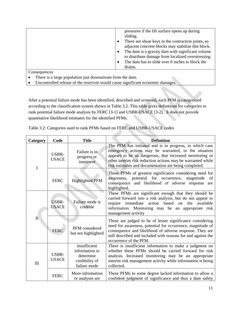
After a potential failure mode has been identified, described and screened, each PFM is categorized according to the classification system shown in Table 3.2. This table gives definitions for categories to rank potential failure mode analysis by FERC [3-1] and USBR-USACE [3-2]. It does not provide quantitative likelihood estimates for the identified PFMs.

Table 3.2: Categories used to rank PFMs based on FERC and USBR-USACE codes

Category Code Title Definition

I

USBR-USACE

Failure is in progress or imminent

The PFM has initiated and is in progress, in which case emergency actions may be warranted, or the situation appears to be so dangerous, that increased monitoring or other interim risk reduction actions may be warranted while risk estimates and documentation are being completed.

FERC Highlighted PFM

Those PFMs of greatest significance considering need for awareness, potential for occurrence, magnitude of consequence and likelihood of adverse response are highlighted.

II

USBR-USACE

Failure mode is credible

These PFMs are significant enough that they should be carried forward into a risk analysis, but do not appear to require immediate action based on the available information. Monitoring may be an appropriate risk management activity

FERC PFM considered but not highlighted

These are judged to be of lesser significance considering need for awareness, potential for occurrence, magnitude of consequence and likelihood of adverse response. They are still described and included with reasons for and against the occurrence of the PFM.

III

USBR-USACE

Insufficient information to

determine credibility of failure mode

There is insufficient information to make a judgment on whether these PFMs should be carried forward for risk analysis. Increased monitoring may be an appropriate interim risk management activity while information is being collected.

FERC More information or analyses are

These PFMs to some degree lacked information to allow a confident judgment of significance and thus a dam safety

12

needed in order to classify

investigative action or analyses can be recommended. Because action is required before resolution the need for this action may also be highlighted.

IV

USBR-USACE

Failure mode is not credible

These PFMs are clearly so remote that the likelihood of failure is negligible, and hence do not need to be carried forward for risk estimates. However, they still need to be documented along with the reasons they are considered to be negligible risk contributors. Monitoring is likely not warranted for these PFMs.

FERC

Failure mode ruled out or is

considered not viable

The candidate PFM is ruled out as a PFM because the team discovers that the physical possibility for the failure mode does not exist. Or the candidate PFM is considered as not a viable one because it is found to clearly be so remote as to be non-credible or not reasonable to postulate based on information available at this time.

Step 4, Develop the Event Tree

An event tree is a graphical representation that provides an efficient way to organize the chronological sequence of events for a particular potential failure mode from the initiating cause on the left, through a series of linked events (nodes or branches), to the failure or no failure condition on the right (see figure 4.1). Each node represents an event or condition with possible outcomes or states that need to exist for failure to ultimately occur or not occur.

Event trees can be developed in a qualitative sense without assigning probabilities and used in a failure-modes-and-effects analysis. The same qualitative event trees can be used and expanded in a quantitative risk analysis. Event trees are easily understood because they portray the chronological sequence of events that must occur for failure to happen. Event trees aid in the decomposition of failure modes. This decomposition aids in understanding the failure mode and also in briefing management.

4.1 Advantages

Event trees have the advantage of being:

• Well suited for displaying the chronological order of events from left to right.

• Well suited for displaying dependencies between events and in which order they occur.

• Able to facilitate communication about assumptions in developing the model.

• Easily understood by managers and engineers.

• Well suited to display details of the problem.

• Drawn on standard computer spreadsheets, specialty software, or by hand.

• Intuitive because the events from left to right are the sequence of events that occur given the previous event or condition to the left.

13

Figure 4.1: Qualitative Event tree. Example of earthquake causing sliding instability

4.2 General Principles

Event trees visually show the sequence of events leading to failure. Event trees can also follow the basic principles of probability theory and can be used to quantify the probability of the failure mode if likelihoods are assigned at each node of the event tree (see figure 4.2). The following list shows how an event tree can be used to quantify risks.

• Each branch from a node must be mutually exclusive from the other events so that there is no overlap in probability between branches. In other words, probabilities for events emanating from a single node of an event tree add to 1.

• Probabilities are positive. There is no such thing as a negative probability.

• The probabilities along each path can be multiplied together from left to right. The product of multiplying probabilities along a path is the probability of occurrence of that event.

• Adding the products of all the failure paths in the event tree for a given initiating condition or event gives the probability of having a failure due to the initiating event.

• The occurrence of every event in the tree is conditional on the event to the left having occurred.

Figure 4.2 illustrates an event tree used to predict the probability of an uncontrolled release of the reservoir given an earthquake of 1 in 50,000 or greater. Probabilities are assigned to each node of the event tree by expert elicitation. The experts judged that given a 1 in 50,000 or greater earthquake, the concrete has a 50% probability of cracking, a 10% probability of cracking through the dam body, a 30%

EarthquakeOccurs Concrete

Cracks

Crack Extends Through Dam Body

Sliding InitiatesAlong Crack

Uncontrolled Release of the Reservoir During the Earthquake Uncontrolled

Release of the Reservoir Occurs After the Earthquake

No

No

No

No

No

Yes

Yes

Yes

Yes

Yes

Damage Level 1Node A

Damage Level 3Node C

Damage Level 2Node B

Damage Level 4Node D

Damage Level 5Node E

Damage But Minor or No Uncontrolled Release

Uncontrolled Release of the Reservoir

14

chance of sliding, an 0.05% chance of an uncontrolled release of the reservoir during the earthquake, and a 20% chance of an uncontrolled release of the reservoir after the earthquake due to damages and potential changes in the dam (uplift, seepage, etc.). The annual likelihood of releasing the reservoir during the earthquake is obtained by multiplying the damage estimates along the event tree: 1/50000 x 0.5 x 0.1 x 0.3 x 0.05 = 1.5x10-8. The annual likelihood of uncontrolled release of the reservoir after the earthquake is obtained by multiplying the damage estimates along another path: 1/50000 x 0.5 x 0.1 x 0.3 x 0.95 x 0.2 = 5.7x10-8. Also notice that the probabilities at each node add up to 1.0: Node A = 0.5 + 0.5 = 1.0, Node B = 0.1 + 0.9 = 1.0, etc.

Figure 4.2: Example of a Qualitative Event Tree with Probability Estimates

Step 5, Hazard Analysis of Dam Site

5.1 Introduction and selection of earthquake rupture forecast and ground-motion-prediction equations

In this step, the analyst defines the earthquake rupture forecast, ground-motion prediction equations and performs the probabilistic seismic hazard analysis (PSHA). PSHA refers here to estimating the probability of exceeding various levels of shaking intensity at a site, given the site’s foundation conditions, its proximity to nearby seismic sources, how frequently those sources produce earthquakes of various magnitudes at various distances from the site, how ground shaking intensity diminishes with distance from the fault, and how foundation rock or soils amplify ground motion from bedrock.

As used here, an earthquake rupture forecast (ERF) is a mathematical model of the spatial locations of all seismic sources in the region, and their magnitude-frequency recurrence relationship. By magnitude-

EarthquakeOccurs Concrete

Cracks

Crack Extends Through Dam Body

Sliding InitiatesAlong Crack

Uncontrolled Release of the Reservoir During the Earthquake Uncontrolled

Release of the Reservoir Occurs After the Earthquake

No

No

No

No

No

Yes

Yes

Yes

Yes

Yes

Damage Level 1Node A

Damage Level 3Node C

Damage Level 2Node B

Damage Level 4Node D

Damage Level 5Node E

Damage But Minor or No Uncontrolled Release

Uncontrolled Release of the Reservoir

0.5

0.5

0.1

0.9

0.3

0.7

0.05

0.95

0.2

0.8

0.3 Numbers indicate probability of occurring

1:50,000

15

frequency relationship, we mean a relationship that shows how frequently an event of magnitude M or greater occurs, as a function of M.

Ground motion prediction equations (GMPEs) are also commonly called attenuation relationships. They provide a means of estimating the ground shaking intensity and its associated uncertainty at any given site or location, based on what measure of ground shaking intensity is desired (e.g., 5% damped elastic spectral acceleration response at some period of interest), an earthquake magnitude, source-to-site distance, local geotechnical conditions, and faulting mechanism (e.g., normal, reverse, or strike-slip). GMPEs are efficiently used to estimate ground motions for use in both deterministic and probabilistic seismic hazard analyses.

The best ERF and GMPEs may evolve over time. As of this writing, an in-progress project is likely to produce authoritative recommendations for both of these model components by March 2013. That project is Earthquake Model of the Middle East (EMME), which can be found at http://www.emme-gem.org/. We expect that EMME’s recommendations will be adopted by the Global Earthquake Model (www.globalquakemodel.org), which will encode both the ERF and GMPEs in open-source software that should be accessible to Enerjisa.

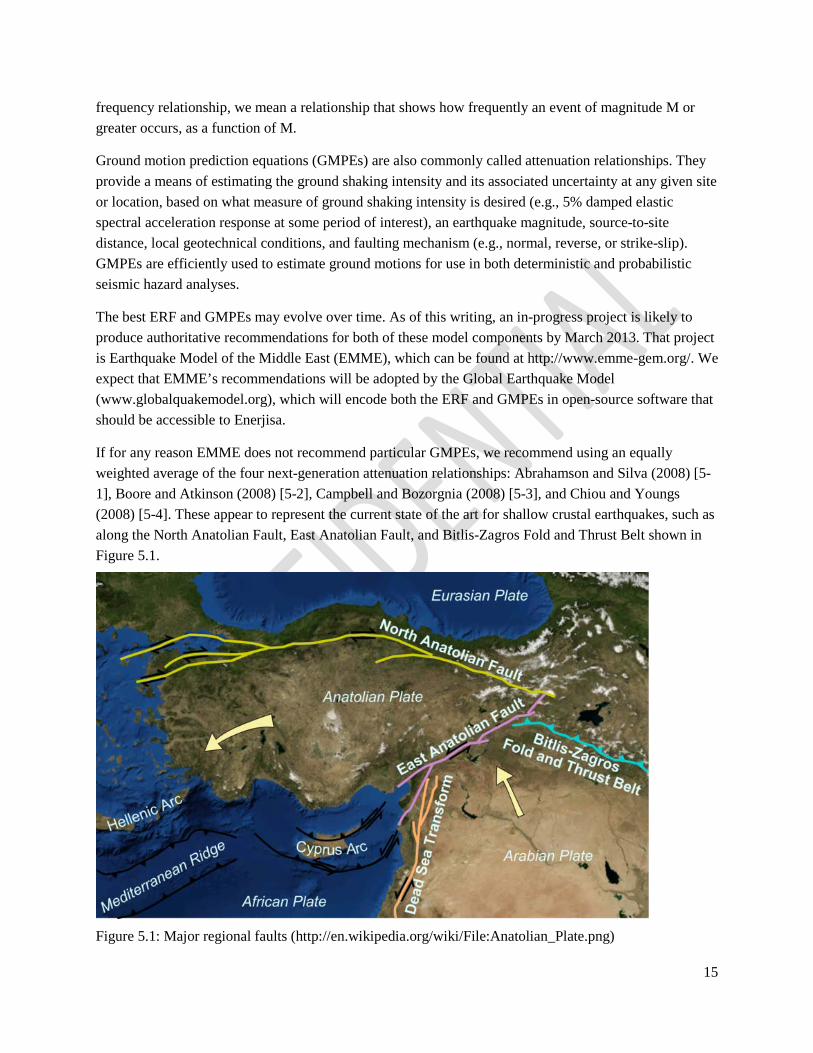
If for any reason EMME does not recommend particular GMPEs, we recommend using an equally weighted average of the four next-generation attenuation relationships: Abrahamson and Silva (2008) [5-1], Boore and Atkinson (2008) [5-2], Campbell and Bozorgnia (2008) [5-3], and Chiou and Youngs (2008) [5-4]. These appear to represent the current state of the art for shallow crustal earthquakes, such as along the North Anatolian Fault, East Anatolian Fault, and Bitlis-Zagros Fold and Thrust Belt shown in Figure 5.1.

Figure 5.1: Major regional faults (http://en.wikipedia.org/wiki/File:Anatolian_Plate.png)

16

The rest of the section extensively quotes Chapter 4 of ATC-58 [5-5] which represents the state of the art with regard to 2nd-generation performance-based earthquake engineering (PBEE-2). It presents earthquake ground shaking characterization procedures. These include development of target spectra and earthquake acceleration time series (ground motions) for use with nonlinear dynamic structural analysis. As discussed in Section 5.4.2, three types of target spectra are acceptable for use here: uniform hazard spectra, conditional mean spectra and conditional spectra.

Dam sites can be subject to other seismic hazards besides shaking that can cause damage and significantly impact performance. These hazards include fault offset at the earth’s surface, liquefaction, lateral spreading, and landslides. While the present document could be expanded to address these other hazards it does not do so at this time. As a minimum, engineers using this methodology should conduct a qualitative assessment of the potential impact of these hazards and, if this impact is found significant acknowledge that performance predicted using this methodology does not include these effects.

Earthquake shaking is completely defined by two orthogonal horizontal components and one vertical component. Ground-shaking intensity is represented here by a series of seismic hazard curves and acceleration response spectra derived from these curves associated with selected exceedance probabilities.

In nonlinear response-history analysis, the effects of shaking are considered by simultaneously evaluating response to ground motion triplets representing shaking effects along each of two principal orthogonal horizontal axes of the dam and the vertical axis. The ground motion triplets are scaled for consistency with the response spectrum that represents the desired ground shaking intensity level. For the simplified analysis addressed here, shaking is characterized by 5% damped elastic spectral acceleration response at the first mode period along each horizontal axis.

Section 5.2 addresses site conditions and location. Section 5.3 introduces ground motion prediction equations. Section 5.4 presents procedures for selecting and scaling ground motions for use with nonlinear dynamic structural analysis.

5.2 Dam Location and Site Conditions

5.2.1 Seismic Environment and Hazard

Earthquake shaking hazards are dependent on site location with respect to causative faults and other seismic sources and, regional and site-specific geologic characteristics. Local topographic conditions (e.g., hills, valleys, canyons) can also modify the character of shaking. Determine from the earthquake rupture forecast whether any part of the dam stands within 500 m of the trace of a known active fault. In such a case, the site is not suitable for construction of a dam. Otherwise, determine from the earthquake rupture forecast the distance from the site to every seismic source within 200 km capable of producing an earthquake of magnitude Mmin or greater (e.g. Mmin = 5.0), and determine from the earthquake rupture forecast its annual frequency of producing such an earthquake at such a distance. By “distance” is meant RRup, the closest distance to the rupture plane, as well as RJB, the closest horizontal distance to the surface projection of the rupture.

17

5.2.2 Location

The assessments recommended here require seismic hazard curves that predict the annual frequency of exceedance of key spectral response parameters. To develop hazard curves, the site’s exact location (longitude and latitude) must be identified. Latitude and longitude should be defined to three decimal places (approximately 100m).

5.2.3 Local Geotechnical Effects

It is assumed here that the dam is founded on rock or hard rock. Rock is defined here consistently with ASCE 7-10 [5-6] Section 20.3, as having shearwave velocity of 760 to 1520 m/sec. Hard rock is defined here as having a minimum shearwave velocity of 1520 m/sec. As a minimum, it will be necessary to have sufficient data to characterize the Site Class in accordance with the ASCE 7-10 Standard (ASCE, 2010) [5-6] so that site coefficients can be assigned. This information will generally include the depth, classification and shear wave velocity of materials in the soil column above bedrock, if the dam is not founded on rock or hard rock

5.3 Ground Motion Prediction Equations

Ground motion prediction equations are used to derive acceleration response spectra, and form the basis for probabilistic seismic hazard analyses used to develop the hazard curves needed here. Ground motion prediction equations provide estimated values of ground shaking intensity parameters, such as peak ground acceleration, peak ground velocity and damped elastic spectral acceleration response at particular structural periods, for user-specified combinations of earthquake magnitude and site-to-source distance (e.g., 7WM from a source 12 km from the site) and other parameters.

Ground motion prediction equations are derived by performing regression analyses of the values of intensity parameters obtained from strong motion recordings of past earthquakes against distance, magnitude and other parameters. Horizontal ground shaking is a vector quantity that varies in orientation and amplitude throughout an earthquake’s duration. Strong motion recordings used to develop ground motion prediction equations are typically obtained from pairs of instruments arranged to capture orthogonal horizontal components of motion. At any instant of time, each component of recorded motion will have different amplitude and neither may be the maximum component of motion that occurred at the given point of time. Most ground motion prediction equations now provide geometric mean (geomean) spectral response accelerations that represent the quantity:

𝑆𝑆𝑔𝑔𝑔𝑔(𝑇𝑇) = �𝑆𝑆𝑥𝑥(𝑇𝑇) × 𝑆𝑆𝑦𝑦(𝑇𝑇) (5-1)

where 𝑆𝑆𝑥𝑥(𝑇𝑇) and 𝑆𝑆𝑦𝑦(𝑇𝑇) are orthogonal horizontal components of spectral response acceleration at period T. The X and Y directions may represent the actual recorded orientations, or may represent a rotated axis orientation. Some equations rotate the motion to capture fault-normal and fault-parallel orientations, while others use an arbitrary rotation intended to capture a maximum orientation. The geomean approximately represents a statistical mean response, with actual shaking response in any direction as likely to be higher as it is lower than the geomean. Maximum response acceleration can be as high as 130% of the geomean while the minimum response acceleration can be less than 80% of the geomean.

18

Except within a few kilometers of the zone of fault rupture, the orientation of maximum spectral response with respect to the stroke of the fault is random and varies with period.

If the site is within 20 to 30 km of the presumed zone of fault rupture and the selected earthquake magnitude is Mw 6 or greater, fault directivity effects should be considered. Fault directivity characterizes whether the progression of rupture along the fault is towards the site or away from the site and can have substantial effect on the amplitude, duration and period content of shaking. Directivity should be specified as: forward directivity (rupture progresses towards the site); reverse directivity (rupture progresses away from the site); null directivity; or unspecified directivity (random direction of rupture progression). NEHRP Consultants (2012A) [5-7] provide guidance on fault-rupture directivity and how to include it in hazard calculations.

At sites located within the forward directivity region, and within 20 km of the rupture zone of large magnitude (Mw 6.0 or greater) strike-slip faulting, shaking in the fault normal direction often exhibits significant velocity pulses as well as significantly larger amplitude than does shaking in the fault parallel direction. This effect is known as directionality. Hazard assessments on sites within this distance should account for these effects.

Some ground motion prediction equations are quite complex and require spreadsheet or other electronic computation tools for proper implementation. The simpler models, often called attenuation relationships can take the basic form:

1 2 3 4ln lnY c c M c R c R γ= + − − + (5-2)

where Y is the median value of the strong-motion parameter of interest (e.g., geometric mean damped elastic spectral acceleration response at a particular period and damping ratio), M is the earthquake magnitude, R is the source-to-site distance, and γ is a standard error term. Additional terms can be used to account for other effects including near-source directivity faulting mechanism (strike slip, reverse and normal), and site conditions.

The Open Seismic Hazard Analysis website, http://www.opensha.org/, provides a ground motion prediction equation plotter (under the dialog box Applications) that can be downloaded from the website and used to generate median spectra and dispersions for the listed relationships including the Next Generation Attenuation relationships used by the US Geological Survey to produce the national seismic hazard maps referenced by ASCE 7-10.

For a particular earthquake scenario and site, different attenuation relationships can provide significantly different estimates of the probable values of spectral response acceleration. These differences result from differences in the data set of records used to develop each relationship and differences in the functional form of the relationships. Figure 5-2 illustrates these differences by presenting the value of 5% damped spectral acceleration response at 0.2-second period, derived using three different relationships for an Mw 7.25 event and an Mw 5.0 event for site-to-source distances ranging from 1 km to 100 km. The differences between ground motion prediction equations are sources of uncertainty associated with determining ground motion intensity for a scenario.

19

Figure 5.2: Illustration of the differences between three ground motion prediction equations

Some prediction equations use shear-wave velocity in the upper 30 m of the foundation as an input variable while others are applicable only for a particular foundation type. If the selected equation has an input variable for shear wave velocity in the upper 30 m, the site-specific value should be used for seismic hazard calculations.

If the selected equation uses a generic description of the reference foundation type (e.g., soft rock6) and reports the reference shear wave velocity, spectra so calculated should be adjusted for the site-specific shear wave velocity in the upper 30 m of the foundation column using either site-response analysis tools or site class factors such as Fa and Fv in ASCE7-10.

Ground motion prediction equations can be used to develop an acceleration response spectrum for a site by repeating the model calculations for many values of period across the range of interest (typically 0.1 to 0.5 second). In addition to uncertainties associated with the differences in response accelerations derived from different attenuation relationships, each equation includes a measure of uncertainty associated with the lack of perfect match between the values predicted by the model and the measured values of acceleration upon which they were based. Some models permit calculation of a distribution of response acceleration values. Figure 5.3 illustrates this with plots of response spectra for different probabilities of exceedance, all derived from a single ground motion prediction equation for an Mw 7.25 earthquake.

6 In which case, mass of the foundation should be accounted and a deconvolution analysis performed per Step 7.

20

Figure 5.3: Response spectra with different probabilities of exceedance derived from a single ground motion prediction equation for an earthquake scenario.

5.4 Selecting and Scaling Motions for Nonlinear Response-History Analysis

5.4.1 Introduction

This section describes recommended procedures for selecting and scaling acceleration histories for use with nonlinear response-history analysis. The basic procedure consists of:

1. Development of an appropriate target acceleration response spectrum;

2. Selection of an appropriate suite of earthquake ground motions; and

3. Scaling of the motions for consistency with the target spectrum.

5.4.2 Target Acceleration Response Spectra

One spectrum is required for each of the several seismic hazard intervals used for analysis. These seismic hazard intervals are selected from the site seismic hazard curve (see Section 5.4.4). Three kinds of spectra are acceptable: (1) uniform hazard spectra, (2) conditional mean spectra or (3) conditional spectra. See ATC-58 Appendix B [5-5] for details on all three types of spectra. For frequent events (high annual frequency of exceedance), the uniform hazard spectrum and conditional mean spectrum should have similar shape. For infrequent events (low annual frequency of exceedance), the amplitude of a conditional mean spectrum will be smaller at some periods than the uniform hazard spectrum as the conditional mean spectrum quantifies a less conservative and more realistic spectrum for a single earthquake. The conditional spectrum differs from the conditional mean spectrum only in that it considers uncertainty in spectral values. The use of either conditional mean spectra or conditional spectra will provide more accurate estimates of response for a given intensity of earthquake shaking than the uniform hazard spectrum, but additional effort is required to generate these types of spectra.

0 1 2 3 4 5Period (sec)

0

0.5

1

1.5

2

2.5S

pect

ral a

ccel

erat

ion

(g)

Boore-Atkinson model,Mw=7.25, r=5 km

97th84thMedian (50th)16th3rd

21

The previous paragraph deals with spectra for horizontal motion. The vertical acceleration response spectrum, denoted here by Sav(T), can be constructed by scaling the corresponding ordinates of the horizontal response spectrum, Sa(T), as follows.

( ) ( )( )( )( ) ( )

( )10

0.1sec

1 1.048 log 1 0.1 0.3sec

0.5 0.3 1.0sec

av a

s

a

S T S T T

T S T T

S T T

= ≤

= − + ⋅ < ≤

= ⋅ < ≤

(5-3)

5.4.3 Scaling Parameters

Ground motions are amplitude scaled to provide acceptable consistency, both individually and in a mean sense, to the target spectrum over a range of structural periods, Tmin to Tmax, as defined below. The dam’s small-amplitude fundamental period of vibration is denoted here by T1. Motions are scaled at this period. After a target spectrum has been defined ground motions are selected and scaled to be consistent with the target spectrum over a period range 𝑇𝑇𝑔𝑔𝑚𝑚𝑚𝑚 to 𝑇𝑇𝑔𝑔𝑚𝑚𝑥𝑥. 𝑇𝑇𝑔𝑔𝑚𝑚𝑥𝑥 is taken as 2T1. Period 𝑇𝑇𝑔𝑔𝑚𝑚𝑚𝑚 should typically be taken as 0.2T1. If substantial response and damage can occur due to response in modes having periods smaller than Tmin, 𝑇𝑇𝑔𝑔𝑚𝑚𝑚𝑚 should be selected to be sufficiently small to capture these important behaviors.

5.4.4 Ground Motion Selection and Scaling

The intent of ground motion selection is to obtain a set of motions that will produce unbiased estimates of structural response when used with nonlinear response-history analysis. When there is significant scatter in spectral shape of the selected records or a poor fit to the target spectrum, eleven or more triplets of motions may be needed to produce reasonable estimates of median response. Use of fewer than 7 motion pairs is not recommended regardless of the goodness of fit of the spectra of the selected motions to that of the target. We denote by n the number of ground motion triplets required for each level of excitation. For simplicity, we recommend n = 11, although more may be used.

Note that n = 11 is selected because it generally produces a reasonable estimate of median structural response (within ±20%) with reasonable confidence (75%), according to Huang et al. (2011) [5-9]. The [5-9] research was performed through nonlinear response-history analysis of a large family of nonlinear single degree-of-freedom (SDOF) oscillators subjected to 50 total pairs of near-fault (1-18 km) and far-field (20-50 km) ground motion time histories of earthquakes with magnitude 6.2 to 7.3. The oscillators could represent buildings or dams. Using n = 11 structural analyses for each level of seismic excitation is practical for many kinds of dams, but may be impractical for arch dams when the analyst lacks access to supercomputing or massively parallel computing resources. In such cases, n = 7 is the lowest value supported by [5-9].

To the extent possible, select triplets of earthquake ground motions whose horizontal components have spectral shape similar to that of the target spectrum over the range of periods (Tmin, Tmax). Additional factors to consider include selecting records having faulting mechanism, earthquake magnitude, site-to-source distance and local geology that are similar to those that dominate the seismic hazard at the

22

particular intensity level, although these are not as significant as the overall spectral shape. Ground motions are available from a number of sources, including http://peer.berkeley.edu/products/strong_ground_motion_db.html and www.cosmos-eq.org. These are appropriate for shallow crustal earthquakes in active tectonic regimes anywhere in the world.

The procedures below focus on acceleration time series. For near-fault sites in the forward directivity region or for dams equipped with velocity-sensitive nonstructural components and systems, ground motion selection and scaling should also consider the amplitude and shape of the scaled velocity time series. Time-based performance assessments utilize seismic hazard curves for 5%-damped elastic spectral acceleration response at a period that approximates the dam’s fundamental period of vibration, denoted here by Sa(T1), and suites of ground motion triplet selected and scaled so that their horizontal motions match spectra derived from the seismic hazard curves over a range of exceedance probabilities, and their vertical motions match the spectra derived from the horizontal spectra as shown in Equation 5-3. The seismic hazard curve includes an explicit consideration of ground motion uncertainty.

Step 1 – Select Intensity Range

Select a range of ground motion exceedance probabilities and corresponding spectral response accelerations, Sa(T1). The intensity range should produce dam response that causes negligible damage at the low end to complete loss at the high end. An acceptable range is:

• Minimum Sa(T1) = Smin = 0.05g

• Maximum Sa(T1) = Smax = Sa associated with annual frequency of exceedance of 0.00002/yr (that is, 1 occurrence in 50,000 years)

Step 2 – Select Analysis Intensities

Structural analysis will be performed at a series of intensities spanning the range of intensities selected in Step 1. To identify the analysis intensities, perform the following steps:

1. Develop a seismic hazard curve for Sa(T1), as described in Box 5-1, below.

2. Compute the spectral accelerations Smin and Smax per Step 1 above.

3. Split the range of spectral acceleration, Smin to Smax into Ne intervals; identify the midpoint spectral acceleration in each interval and the corresponding mean annual frequency of exceedance (See Figure 5-4). For all but concrete arch dams, we recommend Ne = 8. Concrete arch dams tend to require 3D nonlinear dynamic structural analysis, which as of this writing can be very time consuming, so m = 8 may be impractical. In such cases, we recommend Ne = 4.

4. Calculate the mean annual frequency of spectral demand in each interval Δλi from the hazard curve and record these frequencies

5. Develop a target spectrum for the mean annual frequency of exceedance of each midpoint spectral acceleration.

6. For each target spectrum, select and scale suites of n ground motion triplets as follows.

23

6.1 Select a candidate suite of ground motion triplets from available data sets of recorded motions.

6.2 For each ground motion triplet, construct the geomean spectrum for the horizontal components, using equation 5-1 over a range of periods (Tmin, Tmax). Compare the geomean shape with that of the target. Select ground motion horizontal pairs with geomean spectra that are similar in shape to the target response spectrum of Step 1 within the period range of Tmin to Tmax. Discard motions that do not fit the shape of the target spectrum adequately.

6.3 Amplitude-scale all three components of each ground motion triplet by the ratio of Sa(T1) obtained from the target spectrum of Step 1 to the geometric mean Sa(T1) of the recorded components.

Figure 5-4: Example hazard curve showing selection, intensity intervals, midpoints and corresponding mean annual frequencies of exceedance.

Box 5-1 Developing a seismic hazard curve. If we have access to the earthquake rupture forecast and ground-motion prediction equations, but not software to perform the hazard analysis, the seismic hazard curve is estimated as follows:

( ) ( ) ( )( ) ( )( )max, , ,

min

| , ,1 1

, , , , 1f f o f mN M N

Y f m of m M o

Y y f m o f m m o F yλ λ λ= = =

≥ = − + ∆ ⋅ −∑ ∑ ∑ (5-4)

Where

0 0.2 0.4 0.6 0.8 1 1.2 1.4 1.6Earthquake intensity, e (g)

0.0001

0.001

0.01

0.1

1

Mea

n an

nual

freq

uenc

y of

exc

eeda

nce

0.124 0.271 0.419 0.566 0.714 0.861 1.009 1.156

∆e1 ∆e2 ∆e3 ∆e4 ∆e5 ∆e6 ∆e7 ∆e8

e1

e2

e3e4

e5 e6e7 e8

∆λ1

∆λ2

∆λ3

∆λ4∆λ5∆λ6

∆λ7∆λ8

24

( )( )( )ln ,

, ,1 ln ,

ln exp1 aNY a

Y f m oaa Y a

yF y

N

µ

σ=

= Φ

∑ (5-5)

Y = site shaking intensity measure, which here is the 5%-damped elastic spectral acceleration response, the geometric mean of 2 horizontal orthogonal directions, at the dam’s estimated small-amplitude fundamental period of vibration T1.

y = a particular value of Y

λ(Y > y) = mean rate at which the site can experience shaking of intensity y or greater, referred to here as the seismic hazard

f = an index to faults in the earthquake rupture forecast, f = 1, 2, … Nf

Nf = number of faults in the earthquake rupture forecast

m = moment magnitude, in Δm = 0.1-magnitude increments, m = Mmin, Mmin + Δm, Mmin + 2Δm, … Mmax,f

Mmin = minimum magnitude considered, such as 5.0

Mmax,f = maximum magnitude that fault f is believed to be capable of producing, according to the earthquake rupture forecast

o = an index to discrete locations along a fault trace at which earthquake epicenters are discretized, o = 1, 2, … No,f,m

No,f,m = number of discrete locations along fault f at which an earthquake of magnitude m can be centered

( ), ,f m oλ = mean frequency with which fault f can produce earthquakes of magnitude m or greater at

location o, according to the earthquake rupture forecast.

FY|f,m,o(y) = probability that shaking intensity Y ≤ y given an earthquake on fault f of magnitude m with epicenter located at o

a = an index to the ground-motion prediction equations used here, a = 1, 2, … Na

Na = number of ground-motion prediction equations used here. For example, if the 4 next-generation attenuation relationships mentioned earlier are used, Na = 4

Φ = standard normal cumulative distribution function evaluated at the term in parentheses. This document assumes that all ground-motion prediction equations assume that Y is lognormally distributed conditioned on magnitude, distance, mechanism, etc.

μlnY,a = expected value of the natural logarithm of Y under ground-motion-prediction equation a. The form and parameters of the ground-motion-prediction equations vary, and are not repeated here.

25

σlnY,a = total standard deviation of the natural logarithm of Y under ground-motion-prediction equation a

Step 6, Develop Fragility Functions

6.1 Theory

You will need one fragility function for each potential failure mode identified in previous steps. If a potential failure mode can occur to more than one degree (such as slight cracking, moderate cracking, etc.), we will need one fragility function for each possible degree of each potential failure mode.

It should be clarified that fragility functions are independent of the structural analysis of the dam (which will be performed in the next step), however itself may depend on separate “calibration’’ analysis of the entire dam or of a sub-component.

Each fragility function is typically defined completely by two parameter values, θ and β, as explained in more detail below. A fragility function as used here gives the probability that a potential failure mode identified in step 4 occurs, as a function of a demand parameter. A demand parameter is a measure of internal member force (such as shear force) or deformation (such as sliding distance) that is calculated in the structural analyses.

For example, sliding of the dam relative to the foundation may occur when the shear force along a slip surface exceeds the ultimate shear capacity of the slip plane. That shear capacity of the slip plane is typically uncertain, because either or both the friction angle and cohesion are uncertain. Sliding occurs if the demand (shear force) exceeds capacity (the ultimate shear capacity of the failure plane). In any given structural analysis, the demand is deterministic, that is, it is a certain value calculated in the structural analysis, but the capacity is uncertain. Therefore the probability that the failure mode occurs is the probability that the uncertain capacity is less than or equal to the calculated demand. Thus, the fragility function is taken as the cumulative distribution function of the shear capacity of the failure plane.

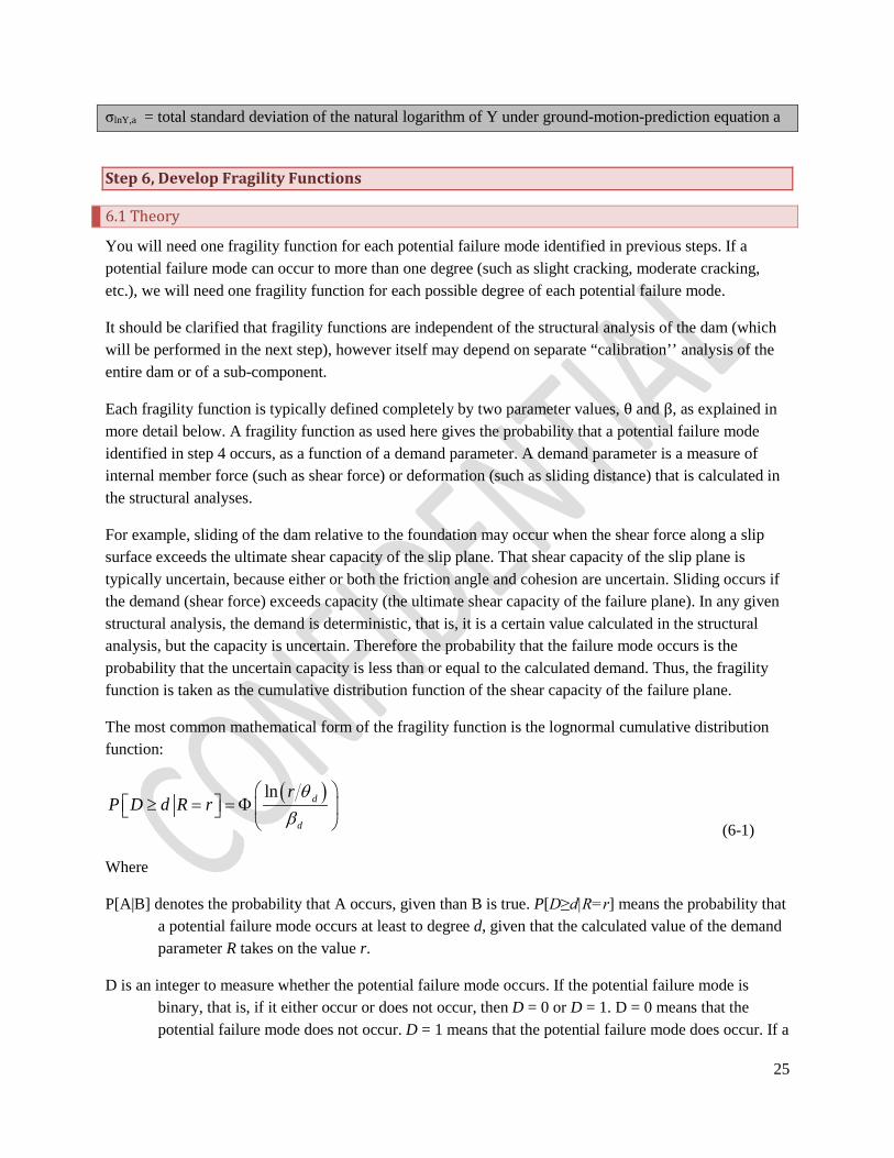
The most common mathematical form of the fragility function is the lognormal cumulative distribution function:

( )ln d

d

rP D d R r

θβ

≥ = = Φ

(6-1)

Where

P[A|B] denotes the probability that A occurs, given than B is true. P[D≥d|R=r] means the probability that a potential failure mode occurs at least to degree d, given that the calculated value of the demand parameter R takes on the value r.

D is an integer to measure whether the potential failure mode occurs. If the potential failure mode is binary, that is, if it either occur or does not occur, then D = 0 or D = 1. D = 0 means that the potential failure mode does not occur. D = 1 means that the potential failure mode does occur. If a

26

potential failure mode can occur in more than one degree, then D = 0 means that it does not occur, D =1 means that it occurs to a low degree, D = 2 means that it occurs to a higher degree, etc.

d is a particular value of D. For a binary potential failure mode, then d is either 0 or 1.

R = the demand parameter, e.g., the shear stress at the base of the dam

r = a particular value of R, e.g., the calculated maximum shear stress along the interface between the dam and the basement soil in a particular structural analysis

Φ = the standard normal cumulative distribution function evaluated at the term in parentheses. It is automatically calculated in various software, for example, the normsdist() function in Microsoft Excel

θd = the median value of capacity, that is the value of R at which there is a 50% chance that the potential failure mode occurs. If the potential failure mode is binary, that is if it either occurs or does not occur, then there is only one θd, denoted simply by θ, and it is the median value of demand at which the potential failure mode occurs. If there is more than one degree possible of the potential failure mode, then there is a θ1, a θ2, and so on, one for each possible degree of the potential failure mode. It is the business of this step in the analysis to determine each of the θ values, and to determine the corresponding β values, discussed next

βd = the logarithmic standard deviation of capacity for degree d of the potential failure mode. It measures how uncertain the capacity is. If the potential failure mode is binary, then there is only one βd, denoted simply by β. The logarithmic standard deviation of capacity is a measure of how uncertain the capacity is. It is typically taken as a number between 0.2 and 0.6. A low value means the uncertain capacity varies only a little, and a high value means that it varies a lot. If you do not know how variable the capacity is, it is reasonable to take β = 0.4, which means that the 10% and 90% probability bounds of the capacity are 0.6 · θ and 1.7 · θ.

Develop a fragility function for each potential failure mode. This means estimate θ and β for each potential failure mode (sliding, overturning, overstressing, foundation failure, cracking, and so on). If a potential failure mode can occur in more than one degree, estimate θ1 and β1, θ2 and β2, etc., one pair for each degree. There are several ways to estimate θ and β: from laboratory tests, from earthquake observations, from expert opinion, and others, [5-8]. The best way to develop a fragility function is from laboratory tests. The simplest way is from expert opinion.

6.2 Case study of seismic fragility function for a concrete gravity dam

In this simple example we seek to derive the fragility function for shear failure. Resistance R is simply R = σ tan(Φ) + c; and Demand: D = τ

where σ and τ are the applied normal stress and shear stress (from analysis). Φ and c are the angle of friction and cohesion. A normal distribution is assigned to both Φ and c with μ(Φ) = 50; and σ(Φ)=3; μ(c)

27

= 10 and σ(c) = 2. A sample size of 10,000 is used. Negative Φ and c values are floored to zero. Through a Monte Carlo simulation, we estimate the probability of failure as the number of occurrences where D > R divided by sample size.

.

Fig. 6-1 Fragility function in terms of a vector of 2 demand parameters

Step 7, Specific Structural Analysis

Written in a separate file,

Step 8, Damage Analysis

In this step, one calculates the probability that each potential failure mode can occur at each level of seismic excitation. In step 5, the analyst produced ground-motion time histories to serve as input to nonlinear dynamic structural analyses. In step 6, the analyst produced the fragility functions that relate the probability that a failure mode occurs to a demand parameter. In step 7, the analyst performed the structural analyses and estimated the demand parameters for each ground motion time history. Now use Monte Carlo simulation (MCS) to estimate probabilistic damage in each nonlinear dynamic structural analysis. Details of MCS as a general procedure can be found in various textbooks of probability and statistics, and online, for example in http://en.wikipedia.org/wiki/Monte_Carlo_method.

28

Here is how to calculate the probability that any individual potential failure mode occurs given the results of any particular structural analysis, and to produce one simulated outcome.

For a binary potential failure mode (it either occurs not), calculate the probability according to Equation 6-1. Then simulate the occurrence or nonoccurrence of the potential failure mode as follows:

Draw a sample value u of random variable that is uniformly distributed between 0 and 1. Mathematically, draw

u ~ U(0, 1) (8-1)

Various software packages can automatically generate a sample of U(0,1). For example, in Microsoft Excel, the function is rand(), where the parentheses are empty. Every time the spreadsheet is recalculated, the value of rand() changes. Then

0 1

1

D if u P D R r

otherwise

= > ≥ = =

(8-2)

where P[ D ≥ 1 | R = r ] is given by the fragility function in Equation 6-1, and refers to the probability that damage occurs (denoted by D ≥ 1) given that the demand parameter R equals a particular value r. Recall that the structural response. Recall that D = 0 indicates that the potential failure mode has not occurred in this particular simulation, and D = 1 indicates that it has. Also recall that the proper demand parameter R to use varies by potential failure mode. For example, to simulate whether sliding occurs relative to the basement rock, R is the shear force at the interface.

There may be cases where there is more than one possible degree of the potential failure mode. Let ND denote the number of possible degrees other than undamaged. They should be sorted in increasing order of severity, that is, D = 1 is the least severe, D = 2 is more severe than D = 1, etc. Again draw u ~ U(0,1). The degree of damage is then taken as

[ ]0 1

max :

D if u P D R r

d u P D d R r

= ≥ ≥ = = < ≥ =

(8-3)

where P[ D≥ d | R = r ] is the failure probability for damage state d, and is calculated for each value of D = 1, 2, … ND using the fragility function in Equation 6-1. That is, the damage state in this simulation is the largest one (the maximum value of d) whose fragility function gives a failure probability that is greater than u. If none of the fragility functions gives a failure probability greater than u, then the potential failure mode does not occur at all, that is, D = 0. Recall that for each value of D, the fragility function in Equation 6-1 requires a pair of parameters θ and β, e.g., θ1 and β1 for damage state 1, θ2 and β2 for damage state 2, etc.

For each structural analysis performed in Step 7, simulate the damage state for each potential failure mode many times. Let Ns denote the number of simulations of damage per structural analysis. We recommend Ns ≥ 100. Thus, for each ground motion time history triplet, simulate Ns vectors of the

29

damage state of for the dam, where the elements in each vector are the damage state (D is one of 0, 1, 2, … ND} for one of the potential failure modes. Remember that ND can vary between potential failure modes.

It is not necessary for this procedure, but can be of interest, to know the probability distribution of each potential failure mode as a function of the level of seismic excitation, e1, e2, … eNe from step 7. For each level of excitation e, calculate the probability distribution of each potential failure mode:

( ),1 1

1 1 sNn

i si ss

P D d E e I D dn N = =

= = = ⋅ ⋅ = ∑∑

(8-4)

Where

n = number of ground motion triplets for each level of excitation selected in Step 7. That is, n is the number of structural analyses performed at each level of seismic excitation, each structural analysis corresponding to a ground-motion triplet. As discussed in Section 5.4.4, we recommended n = 11. For arch dams, n = 7 is the minimum supported by [5-9].

Di,s = simulated value of the potential failure mode’s damage state for ground-motion triplet i, simulation s, at excitation level e

I(Di,s=d) = 1 if D = d, 0 otherwise

Step 9, Loss Analysis

The following concepts have been used by the Bureau of Reclamation since 1996 to estimate the number of fatalities from failure of a dam or appurtenant structures. Recommended fatality rates are used for estimating life loss resulting from dam failure based on [9-1], Table 9.2. The procedure was developed using data from every dam failure in the United States that resulted in more than 50 fatalities and every post-1960 United States dam failure that resulted in 1 or more fatalities. This dam failure data provided information on warning, population at risk, flood severity, and fatality rates. It was concluded that loss of life resulting from dam failure is highly influenced by these factors: 1) the number of people in the inundation area before any evacuation takes place, 2) the amount of warning that is provided to people exposed to dangerous inundation flows, 3) the severity of the inundation flows, and the understanding people in the inundation plain have of the impending severity of the inundation flows.

The failure of a dam can occur from various causes and at different times of the day, week or year. The consequences of dam failure or sudden water releases from the dam are different depending upon the cause of failure or sudden release and when the event occurs. As such, the procedure for estimating loss of life from dam failure is comprised of 7 steps:

1) Determine the level of damage to the dam to evaluate.

2) Determine time categories (i.e. day, week, or year) for which loss of life estimates are needed.

3) Determine the inundation area for each damage scenario.

30

4) Estimate the number of people at risk for each damage scenario and time category.

5) Determine when warnings would be initiated.

6) Select appropriate fatality rate to estimate life loss. The fatality rate is based on the discharge severity, the warning time, and the understanding people in the inundation area have of the severity of the impending discharge as explained below.

7) Evaluate uncertainty through various parameters which lead to uncertainties in the life loss estimates as explained below.

9.1 Severity of the Discharge from an Uncontrolled Release of the Reservoir

The severity of the uncontrolled release of the reservoir through a downstream area determines how much damage can be done and the potential for people to lose their lives. Damage to homes and buildings can be estimated from the depth of flow multiplied by the volume of flow (DV) factor (as defined below), flow depth, and local terrain conditions. For loss of life estimates, categories for discharge severity are:

• Low severity. Low severity occurs when no buildings are assumed to wash off their foundations.

• Medium severity. Medium severity is assumed when homes are destroyed but trees or mangled homes remain for people to seek refuge.

• High severity. High severity is assumed when the discharged sweeps the area clean and nothing remains.

The DV parameter can be used to separate low severity discharge from medium severity discharge where:

𝐷𝐷𝐷𝐷 = 𝑄𝑄𝑑𝑑𝑑𝑑−𝑄𝑄2.33

𝑊𝑊𝑑𝑑𝑑𝑑 (9-1)

Qdf is the discharge at a particular site caused by the damage. Q2.33 is the mean annual discharge at the same site. This discharge can be easily estimated and it is an indicator of the safe channel capacity. As discharges increase above this value, there is a greater chance that they will cause flow over the riverbank. Wdf is the maximum width of discharge caused by damage at the same site. The units of DV are d2/s or depth of flow multiplied by velocity of the flow, thus the term DV. Although the parameter DV is not representative of the depth and velocity at any particular structure, it is representative of the general level of destructiveness that would be caused by the inundation waters. The parameter DV should provide a good indication of the severity (potential lethality) of the uncontrolled release of the reservoir. As the peak discharge from the damage increases, the value of DV increases. As the width of the area of discharge narrows, the value of DV increases. Low discharge severity should be assumed, in general, when DV is less than 5 m2/s. Medium discharge severity should be assumed, in general, when DV is more than this value. However, site specific data (flow depth, terrain, local conditions) should be used when postulating discharge severity and not just DV values alone. The range of DV values for high, medium, and low categories is relatively large and overlaps as shown in Table 9.1.

Table 9.1: DV Values in Reference [9-1] from Case Histories

Discharge Severity DV (ft2/sec) Standard Number of

31

Category Lowest Value Mean Highest Value Deviation Cases High Medium Low

200 25 4

582 150 28

963 357 67

540 98 20

2 19 9

9.2 Warning Time

Warning time is probably the most important factor in saving lives. Sufficient warning time allows people to exit the inundation area, although some people may still lose their lives because they remain in the inundation area or return to the area trying to secure their belongings. For loss of life estimates, categories for warning time are:

• No warning. No warning means that no warning is issued by the media or official sources in the particular area prior to the arrival of inundation flows.

• Some warning. Some warning means officials or the media begin warning in the particular area 15 to 60 minutes before arrival of inundation flows. Some people will learn of the discharge indirectly when contacted by friends, neighbors, or relatives.

• Adequate warning. Adequate warning means officials or the media begins warning in the particular area more than 60 minutes before the water arrives.

9.3 Understanding of the Impending Discharge

Understanding of the impending discharge refers to the relative understanding of people in the inundation area about the severity of the impending flow of water. This affects the desire and willingness for people to leave the inundation area. For loss of life estimates, categories for this severity understanding are:

• Vague. Vague understanding means that the warning issuers have not yet seen actual damage to a dam or do not comprehend the true magnitude of the release of the reservoir.

• Precise. Precise understanding means that the warning issuers have an excellent understanding of the impending discharge due to observations of the discharge made by themselves or others.

9.4 Uncertainties in Estimating Life Loss

Various types of uncertainty can influence loss of life estimates. Quantifying uncertainty is difficult. There is uncertainty associated with various inputs used in this analysis. Factors contributing to uncertainty include the following:

• The rate at which damage occurs and the ultimate size of the damage.

• The breach characteristics including breach time and geometry.

• The depth and velocity of discharge within the inundation area is computed; therefore it is not known if the actual discharge would be severe enough to wash buildings off of their foundations.

• The number of people at risk varies as people depart and arrive from their residences throughout the day.

• When warnings are initiated

32

• The quantity and quality of warnings that are issued.

• Water wave travel times are subject to considerable variation. Existing dam damage computer models can yield varying travel times as input parameters are changed.

• The proper fatality rates to use.

9.5 Example

The following example illustrates the procedure.

Postulate breach scenarios and inundation mapping - Various dam breach and appurtenant structure release scenarios are postulated. This is where Potential Failure Modes characterized in the previous sections help in defining various breach scenarios. Depending on the structures at the site and loading conditions, there may be many breach scenarios. The scenarios are screened and inundation maps developed using say one- or two-dimensional hydraulic simulations using MIKE11-1D and MIKE21-2D from the Danish Hydraulic Institute [9-2]. In this example, there is a concrete gravity dam, a concrete spillway, and an outlet works. Uncontrolled release of the reservoir through a seismically damaged outlet works stays within the safe downstream capacity of the river and is eliminated from further consideration. A seismic event could cause damage to the dam and spillway and cause loss of life. Thus, inundation studies are performed for 2 scenarios: maximum uncontrolled releases through the spillway damaged by an earthquake and uncontrolled releases from a dam breached from a seismic event during normal operating reservoir level.

Populations at Risk – From the inundation maps, populations at risk downstream are determined by the number of people in the inundation area.

Warning time and warning effectiveness - Water wave travel times and depths of flow are estimated. The amount of warning time and the warning time effectiveness is estimated and is a function of when the breach will be discovered, the water wave travel times, and how the downstream populations will be notified.

In our example, the dam is located only a few kilometers upstream from a city. It may be difficult to provide sufficient and forceful warning to residents of the city. It is reasonable to assume that a large percentage of the loss of life resulting from a dam breach would occur. There are no major population centers for many miles downstream from the city; and the communities that are downstream from the city would benefit from more warning time and warnings that would be enhanced with the knowledge of the inundation magnitude as it went through the bigger city. The people exposed to life-threatening discharges in the downstream communities would likely receive warnings that clearly describe the seriousness of the situation.

A rapid uncontrolled release of water from the dam during the day would be noticed almost immediately after failure. There are numerous facilities and people close to the dam. However, before people receive warning, the failure must be noticed, authorities must be contacted, and some form of warning (e.g. sirens, radio, or television) must be initiated. This all takes time. In this case, warn is assumed to start being issued 10 minutes after failure. This may be highly optimistic.

33

Discharge severity – Discharge severity determines if people can run or climb to safety or if the flowing water will wash trees and building off their foundation. In this example, discharge severity is determined for each damage scenario by computing DV at various locations downstream from the dam. The amount of water flow is listed in the inundation study and the discharge width was measured off the inundation maps. Table 9.5 shows the DV values at various distances downstream from the dam for a given damage scenario and the recommended range of high, medium, and low severity for DV values. As can be seen, water flowing through the large city is at a high severity DV, downstream from the city are at a medium severity DV, and 100 miles downstream are at a low severity DV.

Understanding of the Severity of the Discharge – People may or may not evacuate depending on their understanding of the pending water flow. In our example for this potential failure mode, no understanding to vague understanding of the impending water flow was assumed for people in the larger city because of the proximity to the dam. People just downstream from the city may have a vague understanding of the impending water flow. People downstream from this will have over 1.5 hours of warning and should have a precise understanding of the water flow (see Table 9.4 and 9.5).

It can be postulated that maybe vague warning for daytime seismic damage scenarios for areas that would be inundated during the first two hours after the initiation of damage. For nighttime seismic damage scenarios, vague warning was assumed for areas that would be inundated during the first 3 hours after the initiation of damage.

Loss of Life Estimates – Given the above data, loss of life can be estimated in Table 9.6 based on fatality rates in Table 9.2, populations at risk in Table 9.3, assumptions about warning times in Table 9.4, and fatality parameters in Table 9.5. In our example, values for these factors are given for rapid damage occurring during a sunny day.

Table 9.2: Recommended Fatality Rates for Estimating Loss of Life Resulting from Dam Failure

Flood Severity

Warning Time

(minutes)

Flood Severity

Understanding

Fatality Rate – Fraction of people at risk expected to lose their lives

Suggested Suggested Range

High

No warning Not applicable 0.75 0.3 to 1.0

15 to 60 Vague

Use the values shown above and apply to the number of people who remain in

the dam failure flood plain after warnings are issued.

Precise

More than 60 Vague

Precise

Medium No warning Not applicable 0.15 0.03 to 0.35

34

15 to 60 Vague 0.04 0.01 to 0.08

Precise 0.02 0.005 to 0.04

More than 60 Vague 0.03 0.005 to 0.06

Precise 0.01 0.002 to 0.02

Low

No warning Not applicable 0.01 0.0 to 0.02

15 to 60 Vague 0.007 0.0 to 0.015

Precise 0.002 0.0 to 0.004

More than 60 Vague 0.0003 0.0 to 0.0006

Precise 0.0002 0.0 to 0.0004

Note: There is no guidance provided on how many people will remain in the flood plain.

Table 9.3: Number of People at Risk for Example Problem

Location Seismic Day Night

Reach 1 - Upstream from City (mile 0.0 to 5.0) 39 39 Reach 2 - City (mile 5.0 to 10.4) 8690 8690 Reach 3 - Downstream from City (mile 10.4 to 17.0) 1580 1580 Reach 4 – Farther Downstream from City (mile 17.0 to 32.0) 900 900

Table 9.4: Assumptions about Initiating Warnings for Example Problem

Seismic Day Night

0.25 hour after dam failure 0.5 hour after dam failure

Table 9.5: Fatality Parameters by Reach for Example Problem

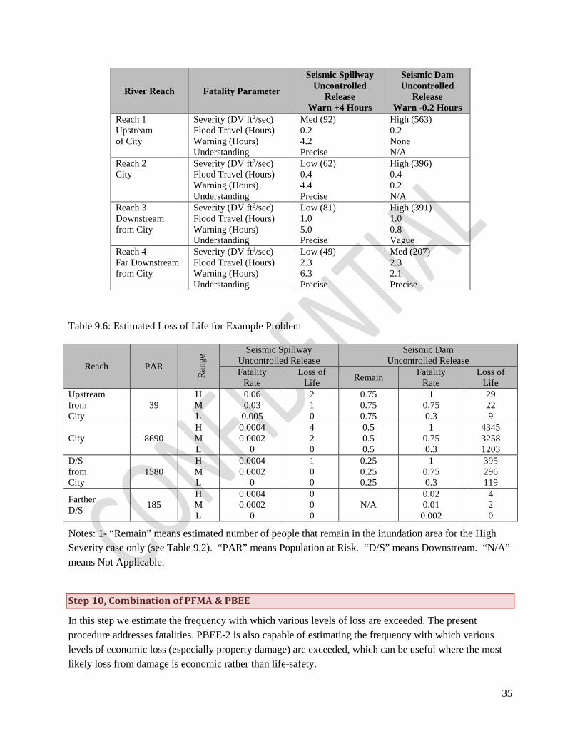
35

River Reach Fatality Parameter

Seismic Spillway Uncontrolled

Release Warn +4 Hours

Seismic Dam Uncontrolled

Release Warn -0.2 Hours

Reach 1 Upstream of City

Severity (DV ft2/sec) Flood Travel (Hours) Warning (Hours) Understanding

Med (92) 0.2 4.2 Precise

High (563) 0.2 None N/A

Reach 2 City

Severity (DV ft2/sec) Flood Travel (Hours) Warning (Hours) Understanding

Low (62) 0.4 4.4 Precise

High (396) 0.4 0.2 N/A

Reach 3 Downstream from City

Severity (DV ft2/sec) Flood Travel (Hours) Warning (Hours) Understanding

Low (81) 1.0 5.0 Precise

High (391) 1.0 0.8 Vague

Reach 4 Far Downstream from City

Severity (DV ft2/sec) Flood Travel (Hours) Warning (Hours) Understanding

Low (49) 2.3 6.3 Precise

Med (207) 2.3 2.1 Precise

Table 9.6: Estimated Loss of Life for Example Problem

Reach PAR

Ran

ge Seismic Spillway

Uncontrolled Release Seismic Dam

Uncontrolled Release Fatality

Rate Loss of

Life Remain Fatality Rate

Loss of Life

Upstream from City

39 H M L

0.06 0.03

0.005

2 1 0

0.75 0.75 0.75

1 0.75 0.3

29 22 9

City 8690 H M L

0.0004 0.0002

0

4 2 0

0.5 0.5 0.5

1 0.75 0.3

4345 3258 1203

D/S from City

1580 H M L

0.0004 0.0002

0

1 0 0

0.25 0.25 0.25

1 0.75 0.3

395 296 119

Farther D/S 185

H M L

0.0004 0.0002

0

0 0 0

N/A 0.02 0.01

0.002

4 2 0

Notes: 1- “Remain” means estimated number of people that remain in the inundation area for the High Severity case only (see Table 9.2). “PAR” means Population at Risk. “D/S” means Downstream. “N/A” means Not Applicable.

Step 10, Combination of PFMA & PBEE

In this step we estimate the frequency with which various levels of loss are exceeded. The present procedure addresses fatalities. PBEE-2 is also capable of estimating the frequency with which various levels of economic loss (especially property damage) are exceeded, which can be useful where the most likely loss from damage is economic rather than life-safety.

36

In each simulation in Step 8, the damage state for each potential failure mode was simulated. For each damage state of each potential failure mode that can result in an uncontrolled release of water, estimate the probability distribution of the number of fatalities that would result. In the following, it is assumed that the lognormal distribution is a reasonable model of the number of fatalities conditioned on the occurrence of a particular potential failure mode and damage state. The analyst is free to assume some other distribution if it seems more reasonable. To estimate the lognormal distribution, it is sufficient to do the following:

From Step 9, estimate L50, the median number of fatalities, i.e., the number of fatalities that exceeded in 5 out of 10 cases.

From Step 9, estimate L90, the number of fatalities that would be exceeded in only 1 out of 10 cases.

Calculate βL as follows

( )90 50ln1.28L

L Lβ = (10-1)

The probability that at least l fatalities occur, given the occurrence of the potential failure mode and damage state is then given by

( )50ln

1L

l LP L l D d

β

≥ = = −Φ

(10-2)

Tabulate L50 and βL for each potential failure mode and damage state that could result in an uncontrolled release of water.

For each structural analysis and each damage simulation each performed in Step 11, simulate the number of fatalities for each potential failure mode i, as follows:

( )( )1

50 exp

0i Ll L u if D d

otherwise

β −= ⋅ ⋅Φ =

= (10-3)

The simulated number of fatalities for a given structural analysis and a given damage simulation is the largest number of fatalities for all potential failure modes, i.e.,

{ }max il l= (10-4)

where

li = fatalities simulated using Equation (10-3) for potential failure mode i.

l = fatalities for a particular structural analysis and damage simulation from Step 8.

37

Note that Equation (10-4) assumes that fatalities from different potential failure modes do not add. That is, it assumes that the people at risk are the same in each potential failure mode, that the occurrence of two or more potential failure modes either kills or does not kill those people, rather than the occurrence of one potential failure mode killing one group of people and the occurrence of another potential failure mode killing a different group of people. Equation (10-4) aims to avoid double-counting fatalities.

Now select five values of total fatalities whose exceedance frequency is desired. We recommend using L0 = 1, L1 = 10, L2 = 100, L3 = 1,000, L4 = 10,000, or generally Lj = 10j, j = 0, 1, 2, 3, 4. For each value of j, calculate f(Lj), meaning the frequency with which at least Lj fatalities occur. It is estimated as:

( ) ( ), ,1 1 1

1e sN Nn

j k i s j kk i s s

f L I l Ln N

λ= = =

= ≥ ∆⋅∑∑∑ (10-5)

Where

j = an index to fatality levels j = {1, 2, 3, 4} k = an index to shaking intensity levels k = {1, 2, … Ne} of Section 5.4.4 Step 2 and Figure 5-3 s = an index to simulation number at a given ground motion intensity level and ground motion triplet Ns = number of simulations per ground motion triplet i = an index to ground motion triplets n = number of ground motion triplets per shaking intensity level I( ) = 1 if the expression in parentheses is true, 0 otherwise Δλk = occurrence frequency of shaking intensity ek, from Sec 5.4.4, Step 2 and Figure 5-3 lk,i,s = number of fatalities simulated in shaking intensity level k, ground motion triplet i, simulation number s

Step 11, Decision

There are various agencies that have established risk-based dam safety decision guidelines. These agencies include the Bureau of Reclamation and the Corps of Engineers in the United States. Similar guidelines have been developed in Australia and Canada. A detailed review of these guidelines is found in the accompanying report [0-1]. Section 11.9 provides our recommended acceptance criteria.

11.1 Bureau of Reclamation Guidelines

Reclamation published interim guidelines [11-1]. Portions of this report are extracted directly from the guideline to accurately represent the intent of the guidelines in this document.

Reclamation uses two guidelines to assess dam safety risk. The first guideline addresses Annualized Failure Probability (annual probability of the loading times the probability of failure given the load), which serves to fulfill the public trust responsibility associated with agency exposure as a result of dam failures (dams should not fail frequently even if the consequences are low). The second guideline addresses Annualized Life Loss (annualized failure probability times the consequences), where multiple fatalities are possible as the result of dam failure. Protection of human life is of primary importance to public agencies constructing, maintaining, or regulating public works.

38

11.2 Annualized Failure Probability

There is no such thing as a dam with zero chance of failure. However, to protect society and to maintain public trust, the probability of dam failure must be very low. This ensures a minimum level of safety when the consequences are not high. For example, Reclamation terms this measure of risk Annualized Failure Probability, and uses a guideline of 1in 10,000 per year for the accumulation of failure likelihoods from all potential failure modes that would result in life-threatening unintentional release of the reservoir. When the mean estimate is above this threshold level there is generally increasing justification to take action to reduce or better understand the risks. Below this threshold level there is generally decreasing justification to reduce or better understand the risks. This guideline is shown as a horizontal line at 10-4 on the risk guidelines chart (Figure 11.1).

11.3 Annualized Life Loss

Society is increasingly averse to hazards as the scale of the consequences (especially the number of people killed) increases. Reclamation defines this risk as Annualized Life Loss, and uses a guideline of 0.001 fatalities per year to address this measure of risk. When the mean estimate is above the guideline of 0.001 fatalities per year, there is generally greater need to take action to reduce or better understand the risks. There is generally decreasing need to reduce or better understand the risks when they are below this guideline value. The primary means to portray risks is a risk curve that relates frequency f (mean number of events per year) of L or more fatalities, as a function of L. We refer to this chart as the risk curve or f-L chart. In the chart, risks associated with individual potential failure modes are plotted as well as the total risk. The guidelines are applied to individual potential failure modes when dominated by a single failure mode or the summation of failure mode risks when several plot near the guidelines. Figure 11.1 illustrates the risk guideline chart. The annualized failure probability multiplied by the estimated lives lost represents the annualized life loss. As the consequences increase by an order of magnitude, the annualized probability must decrease by an order of magnitude to remain tolerable.

11.4 Low Probability – High Consequence Events

Decisions related to failure of structures for remote loading conditions or failure probabilities, combined with high consequences, have been difficult for both decision-makers and risk estimators. Extrapolation of seismic and hydrologic hazards into remote areas is costly and results in loadings where the basis for the results becomes highly uncertain. Predicting events or failure probabilities that are expected to be less probable than 1 in 1,000,000 per year becomes less defendable and uncertainty becomes a major factor when considering potential decisions.

Structures that have the potential to cause more than 1,000 fatalities are generally large in size, highly visible, important to the local community, the region, and the economy. These high profile structures generally receive added attention during all parts of the risk management process by both decision-makers and technical staff. The existence of structures that have the potential to cause major catastrophes indicates that the trade-off between the hazards posed by the structure and the benefits secured by it should be demonstrated with a higher degree of defensibility. However, the profession’s current ability to demonstrate failure probabilities to very low levels, less than 1 in 1,000,000 per year, is limited. This does not mean that these risks should be ignored or that an attempt should not be made to obtain the best

39

information possible in these cases. The opposite is true, although the costs of obtaining the information should be carefully weighed against the potential to gain useful information that could be used to support a decision. As-low-as-reasonably-practicable (ALARP) principles should be considered and weighed against the residual risks posed by the structure.

The chart in Figure 11.1 includes an area bounded by 1 x 10-6 annualized failure probability on the top and 1,000 fatalities on the left. This ‘box’ is shown to indicate that ALARP principles should be considered and additional interaction should occur between the decision-makers and the risk estimators when the risks are thought to be in this region.

Figure 11.1: Generic Dam Safety Risk Guidelines f-L Chart

11.5 Dam Safety Priority Rating

The guidelines for analyzing and portraying risk are used to help guide whether actions are justified or not; they do not establish the priority or urgency of actions. As a general rule, as the annualized failure

1.E-08

1.E-07

1.E-06

1.E-05

1.E-04

1.E-03

1.E-02

1.E-01

0 1 10 100 1,000 10,000

f, ea

rthq

uake

s per

yea

r cau

sing

dam

failu

res w

ith a

t lea

st L

fata

litie

s

L, number of fatalities due to dam failure

Risks are unacceptable, except in exceptional circumstances

Risks are tolerable onlyif they satisfy the ALARP requirements

Limit of tolerability for existing dams

Limit of tolerability for new dams or major augmentations

40

probability and annualized life loss increase, the justification and urgency to take action also increase. Similarly, as the annualized failure probability and annualized life loss decrease, the justification and urgency to take action also decrease. Strive to develop consistent risk estimates through established methodology and review. Recognize that risk estimates are likely to come from a variety of sources. Complete consistency in the estimates cannot be expected. Therefore, the risk numbers by themselves may not be the best way to prioritize activities. To help prioritize and establish the urgency of risk management activities, a Dam Safety Priority Rating (DSPR) system has been adopted by US agencies to assist with these decisions. DSPR ratings apply to dams and not to the individual potential failure modes at a dam. The categorization of a dam is dynamic over time, changing as project characteristics are modified or more refined information becomes available, affecting the loading, annualized failure probability, or consequences of failure.

The DSPR system in Table 11.1 presents different levels of urgency and commensurate actions. These actions range from immediate recognition of a critical situation, in which there is extreme confidence, requiring extraordinary and immediate action for high risk dams through normal operations and routine dam safety activities for dams with low perceived risks at a high confidence level.

11.6 Design Requirements for New Structures and Dam Safety Modifications

When new structures are proposed to be added to an owner’s inventory of dams or when existing structures are proposed to be modified or the operations changed in a way that would potentially change the risks, the proposed designs or operations must be evaluated relative to the dam safety public protection guidelines. This applies to:

• Significant changes to reservoir operations;

• Increases in the maximum water surface elevation for existing structures;

• Modifications to dams for the purposes of dam safety;

• Modifications to dams for purposes other than dam safety, and;

• New dams and appurtenant structures.

It is desirable that changes at dams are risk-neutral; that is that there is no appreciable increase in risk. Ultimately, decision-makers must decide if any increases in risk are acceptable. Often this will involve considering the benefits of the proposed changes versus an increase in dam safety risk. Considerations in evaluating increases in risk for individual potential failure modes should include:

• The magnitude of the baseline risk (an increase for a potential failure mode that has a low baseline risk may be more acceptable than an increase in risk for a potential failure mode where the baseline risk is near the guideline values).

• The potential to add design features or modifications to offset or eliminate risk for specific potential failure modes.

41

• The total risk and the potential to offset an increase in risk for one potential failure mode by reducing the risk for a different potential failure mode.

Generally if significant increased risk is estimated for a proposed change at one of the dams, and the increased risk cannot be mitigated, the proposed change will not be acceptable.

11.7 Design Standards

Once decisions have been made to take action to reduce risk at the facilities, corrective action alternatives are developed to accomplish the desired amount of risk reduction. Although the magnitude of risk reduction varies from project to project, the design methods used to develop these alternatives must consider the agency’s appropriate design standards and state-of-the-art methods used by the dam engineering industry. While these design standards invariably apply to new structures, in the case of dam safety modifications it may not be possible to completely incorporate them without essentially tearing down the structure and starting over. There may be other cost effective methods to reduce risk that follow sound engineering principles which can be considered in such cases.

11.8 Risk Reduction Guidelines

Although the design standards and standard industry methods include many characteristics that have been proven successful and prudent for individual aspects of design and construction, it should be recognized that these standards do not evaluate the effectiveness of engineering systems. Furthermore, lessons learned from incidents and failures of dams have shown that robustness should be an important consideration when designing and constructing dams and appurtenant structures to perform well over time. A risk informed process evaluates the system effectiveness and robustness of designs.

Table 11.1: Dam Safety Priority Rating (DSPR)

Dam Safety Priority Rating Characteristics and Prioritization Considerations Potential Actions

– IMMEDIATE PRIORITY

An active failure mode is in process or the likelihood of a failure is judged to be extremely high, such that immediate actions are necessary to reduce risk.

TOTAL ANNUALIZED LIFE LOSS OR TOTAL FAILURE PROBABILITY IS EXTREMELY HIGH WITH HIGH CONFIDENCE To assign this category consider if:

1. There is direct evidence that failure is in progress and the dam is almost certain to fail if action is not taken quickly.

2. Both the failure probability and the annualized life loss are extremely high.

3. The annualized life loss or failure probability is driven by a single failure mode.

4. The annualized life loss or failure probability is driven by potential failure modes manifesting during normal operating conditions.

- Take immediate action to avoid failure.

- Implement interim risk reduction measures including operational restrictions, and ensure that emergency action plan is current and functionally tested for initiating event.

- Conduct heightened monitoring and evaluation.

- Expedite investigations and designs to support long-term risk reduction.

- Initiate intensive management and situation reports.

2 – URGENT PRIORITY

Potential failure mode(s) are judged to present very serious risks, either due to a very

TOTAL ANNUALIZED LIFE LOSS OR TOTAL FAILURE PROBABILITY IS VERY HIGH WITH HIGH CONFIDENCE OR SUSPECTED OF BEING VERY HIGH TO EXTREMELY HIGH WITH LOW TO

Consider implementing interim risk reduction measures, including operational restrictions as justified, and ensure that emergency action plan is current and functionally tested for

42

high probability of failure or due to very high annualized life loss, which justify an urgency in actions to reduce risk.

MODERATE CONFIDENCE

To assign this category, as well as prioritize dams within this category, consider if:

5. Both the failure probability and the annualized life loss are very high to extreme.

6. The annualized life loss or failure probability is driven by a single failure mode.

7. The annualized life loss or failure probability is driven by potential failure modes

manifesting during normal operating conditions.

8. The range in risk estimates is tightly clustered and the mean and median are similar (for detailed uncertainty analysis only) and/or sensitivity studies instill confidence.

9. Risk reduction or confirmation is relatively easy and inexpensive.

initiating event.

Conduct heightened monitoring and evaluation if appropriate.

Expedite confirmation of rating, as required.

Give very high priority for investigations and designs to support remediation, as required.

3 – MODERATE TO HIGH PRIORITY

Potential failure mode(s) appear to be dam safety deficiencies that pose a significant risk of failure, and actions are needed to better define risks or to reduce risks.

MODERATE TO HIGH TOTAL ANNUALIZED LIFE LOSS OR TOTAL FAILURE PROBABILITY WITH AT LEAST MODERATE CONFIDENCE

To assign this category, as well as prioritize dams within this category, consider if:

10. Both the failure probability and the annualized life loss are moderate to high.

11. The annualized life loss or failure probability is driven by a single failure mode.

12. The annualized life loss or failure probability is driven by potential failure modes manifesting during normal operating conditions.

13. The range in risk estimates is tightly clustered and the mean and median are similar (for detailed uncertainty analysis only) and/or sensitivity studies instill confidence.

14. Risk reduction or confirmation is relatively easy and inexpensive.

Consider whether implementation of interim risk reduction measures is appropriate, which may include ensuring that emergency action plan is current and functionally tested for initiating event; conducting heightened monitoring and evaluation; and in some cases even operational restriction.

Prioritize investigations to support justification for remediation and remediation design, as appropriate

4 – LOW TO MODERATE PRIORITY

Potential failure mode(s) appear to indicate a potential concern, but do not indicate a pressing need for action.

LOW TO MODERATE TOTAL ANNUALIZED LIFE LOSS AND TOTAL FAILURE PROBABILITY WITH LOW CONFIDENCE AND THE REALISTIC POTENTIAL TO MOVE THE ESTIMATE INTO “HIGH”; OR MODERATE TO HIGH TOTAL ANNUALIZED LIFE LOSS AND TOTAL FAILURE PROBABILITY WITH LOW CONFIDENCE AND THE REALISTIC POTENTIAL TO MOVE THE ESTIMATE INTO “LOW”

To assign this category, as well as prioritize dams within this category, consider if:

15. The failure probability and annualized life loss are near guidelines

16. The likelihood that refinement

Ensure routine risk management activities are in place.

For those actions for which the case has been built to proceed before the next comprehensive review, take appropriate interim measures and schedule other actions as appropriate.

Determine whether action can wait until after the next comprehensive review of the dam and appurtenant structures.

43

5 – LOW PRIORITY

Potential failure mode(s) at the facility do not appear to present significant risks, and there are no apparent dam safety deficiencies.

LOW TOTAL ANNUALIZED LIFE LOSS AND TOTAL FAILURE PROBABILITY WITH

MODERATE TO HIGH CONFIDENCE

The annualized life loss and failure probability are estimated to be low and are unlikely to change with additional investigations or study.

Continue routine dam safety risk management activities, normal operation, and maintenance.

11.9 Recommended Acceptability Criteria

The design of a new dam is acceptable if all points on its risk curve (calculated using Equation 10-5) lie inside the limit of tolerability for new dams and major augmentations in Figure 11.1. The design of a major augmentation to an existing dam is acceptable if all points on its risk curve lie inside the limit of tolerability for new dams and major augmentations in Figure 11.1, and no point on the risk curve for the augmented dam is above the risk curve for the dam prior to the augmentation. The design of an existing dam is acceptable if all points on its risk curve lie inside the limit of tolerability for existing dams in Figure 11.1.

12. References

[0-1] Hariri Ardebili, M. and Saouma, V. (2012) Performance Based Seismic Design of Concrete Dams; Background Information, Report submitted to Enerjisa.

[2-1] Federal Energy Regulatory Commission, Engineering Guidelines for the Evaluation of Hydropower Projects, Chapter 14, “Dam Safety Performance Monitoring Program,” 2005.

[3-1] FERC Guidance Document: POTENTIAL FAILURE MODE ANALYSIS, Draft Version, 2005, Federal Emergency Regulatory Committee

[3-2] Selecting Analytic Tools for Concrete Dams to Address Key Events along Potential Failure Mode Paths, 2011, Federal Emergency Management Agency, Denver, Colorado

[5-1] Abrahamson, N., and W. Silva, 2008. Summary of the Abrahamson & Silva NGA Ground-Motion Relations. Earthquake Spectra, 24 (1), 67–97

[5-2] Boore, D.M. and G.M. Atkinson, 2008. Ground-motion prediction equations for the average horizontal component of PGA, PGV, and 5%-damped PSA at spectral periods between 0.01 s and 10.0 s. Earthquake Spectra. 24 (1), 99-138

[5-3] Campbell K.W. and Y. Bozorgnia, 2008. NGA ground motion model for the geometric mean horizontal component of PGA, PGV, PGD and 5% damped linear elastic response spectra for periods ranging from 0.01 to 10s. Earthquake Spectra 24 (1), 139-171

[5-4] Chiou, B.S.J. and R.R. Youngs, 2008. An NGA model for the average horizontal component of peak ground motion and response spectra. Earthquake Spectra, 24 (1), 173-216

44

[5-5] (ATC) Applied Technology Council, 2012. ATC-58: Guidelines for Seismic Performance Assessment of Buildings, 100% Draft. Redwood City, CA.

[5-6] (ASCE) American Society of Civil Engineers, 2010. Minimum Design Loads for Buildings and Other Structures, SEI/ASCE 7-10. Reston VA, 608 pp.

[5-7] NEHRP Consultants Joint Venture, 2011, Soil-Foundation-Structure Interaction for Building Structures, Report No. NIST GCR 11-xxx-x, National Institute of Standards and Technology, Gaithersburg, MD

[5-8] Porter, K., Kennedy, R., Bachman, C. (2007) Creating fragility functions for performance-based earthquake engineering. Earthquake Spectra, 23 (2), 471–489. http://www.sparisk.com/pubs/Porter-2007-deriving-fragility.pdf

[5-9] Huang, Y.N., Whitaker, A.S., Luco, N., Hamburger, R. (2011) Scaling earthquake ground motions for performance-based assessment of buildings. Journal of Structural Engineering, 137 (3) 311-321

[6-1] Tekie, P.B. and Ellingwood, B., 2002. Fragility Analysis of Concrete Gravity Dams, Prepared for U.S. Army Corps of Engineers at Washington DC, Report No. ERDC/ITL TR-02-6, Sep 2002.

[6-2] Tekie, P.B. and Ellingwood, B., 2003, Seismic fragility assessment of concrete gravity dams, Earthquake Engineering and Structural Dynamics, 32, pp.2221-2240.

[6-3] U.S. Bureau of Reclamation, 2005. Quantitative Risk Analysis Using Fragility Curves For Concrete Gravity Dams, Report No. DSO 05-01, Jan 2005, Denver, Colorado.

[9.1] A Procedure for Estimating Loss of Life Cause by Dam Failure,” by Wayne J. Graham, Report No. DSO-99-06, US Bureau of Reclamation, September, 1996.

[9.2] Danish Hydrologic Institute (DHI) (2003): A Modelling System for Rivers and Channels, Hørsholm, Denmark, 2003.

[11-1] Bureau of Reclamation (2011), Dam Safety Public Protection Guidelines – A Risk Framework to Support Dam Safety Decision-Making”

13. Relationship between this document and RFP

Enerjisa Questions Where Covered in this Report

What should be the earthquake load(s)*

1 What studies need to be completed Introduction, Step 1, Step 2

2 How information is to be synthesized Step 3 , Step 4, Step 9

3 What will be the final decision tool Step 11

4 How the findings are to be converted into alternatives for Enerjisa decision-makers Step 11

45

5 Tool for deriving the financial implications of alternatives Step 10

6 Potential damage implication assessment procedure Step 8

7 Technical decision tool for selecting design earthquake magnitude Step 5.3

8 Determination of the types of studies and technical specifications to be completed for quantifying seismic risk

Step 5, (Step 8)

9 Governing fault selection criteria Step 5.1

How should the units be analyzed for given earthquake load(s)

10 Governing design codes and which of their sections Step 5.2 & Step 5.3

11 Analysis methods for respective structures* Step 7 & Step 5.4

12 Material modeling and laboratory testing Step 7

13 Hazard assessment preparation standards Step 5, (Step 6)

14 Fault identification standards Step 5.1

What should be the performance of the units for this earthquake load?*

15 Dam body

Step 11 16 Appurtenant structures

17 Slopes * Refer to the main questions raised by Enerjisa The problem is that with all ranges of loads, methods and performance levels available we are almost always having a hard time deciding in the eq.-resistant design process. This to us is the greatest challenge of all. The questions that we would like to have answered consist of three main ones. We are having a difficult time in deciding what eq. magnitude to select in our designs. This is the first and foremost problem. A 1%, 2%, 5% or etc. event AND why? The other two are what analysis methods we ought to employ and what should be the objective structural performance level.