SEISMIC PERFORMANCE OF CIRCULAR CONCRETE …

SEISMIC PERFORMANCE OF CIRCULAR CONCRETE

FILLED STEEL TUBE COLUMNS FOR

ACCELERATED BRIDGE

CONSTRUCTION

by

Catherine Tucker

A thesis submitted to the faculty of

The University of Utah

in partial fulfillment of the requirements for the degree of

Master of Science

Department of Civil and Environmental Engineering

The University of Utah

August 2014

T h e U n i v e r s i t y o f U t a h G r a d u a t e S c h o o l

STATEMENT OF THESIS APPROVAL

The thesis of Catherine Tucker

has been approved by the following supervisory committee members:

Luis Ibarra , Chair May 9, 2014

Date Approved

Chris Pantelides , Member May 9, 2014

Date Approved

Amanda Bordelon , Member May 9, 2014

Date Approved

and by Michael Barber , Chair/Dean of

the Department/College/School of Civil and Environmental Engineering

and by David B. Kieda, Dean of The Graduate School.

ABSTRACT

This study evaluates the seismic performance of circular concrete filled tube

(CCFT) columns in accelerated bridge construction (ABC) projects. CCFT components

are considered of interest for bridges subjected to seismic forces due to their efficient

structural behavior under combined axial and bending loads: lateral stiffness of the steel

tube is increased by the concrete and concrete confinement is provided by the steel tube.

This research addresses the ability of CCFT columns to perform adequately under

gravitational and seismic loading before the concrete reaches its design strength. A

reduced seismic hazard that accounts for this temporal condition is also implemented.

Performance evaluation is based on the probability of failure of the CCFT column.

For this research, a Caltrans bridge used in previous Pacific Earthquake

Engineering Research Center (PEER) studies is adopted. The performance of a proposed

CCFT column was compared to the original circular reinforced concrete (RC) column.

Numerical analyses using concentrated plasticity models in OpenSees were used for this

evaluation. Experimental data were used to calibrate the deteriorating response of CCFT

columns in OpenSees. The analytical model predicts the CCFT column’s behavior under

monotonic, static cyclic, and dynamic (seismic) loading. Then, the model was adapted to

consider the effects of partial concrete compressive strength on the column behavior. The

study accounts for temporary conditions, such as concrete compressive strength lower

than the design value, and reduced seismic loads. The results indicate that CCFT columns

iv

with partial design concrete compressive strength can be used for ABC because the

relatively low decrease in strength is offset by the reduced seismic loads for this temporal

condition.

dedicated to Elisabeth and Peter

TABLE OF CONTENTS

ABSTRACT ....................................................................................................................... iii

LIST OF FIGURES ......................................................................................................... viii

LIST OF TABLES ............................................................................................................. xi

LIST OF SYMBOLS ........................................................................................................ xii

LIST OF ABBREVIATIONS .......................................................................................... xvi

ACKNOWLEDGEMENTS ........................................................................................... xviii

INTRODUCTION .............................................................................................................. 1

Background and Motivation ................................................................................... 2

Statement of Problem .............................................................................................. 4 Scope and Objectives .............................................................................................. 4 Methodology ........................................................................................................... 5

LITERATURE REVIEW ................................................................................................... 7

Seismic Behavior of Concrete Filled Steel Tube Columns .................................... 7 Slenderness Ratio .............................................................................................. 8 Concrete Confinement ...................................................................................... 9 Composite Action ............................................................................................. 9

Time-Dependent Behavior of Concrete ................................................................ 11 Temporary Conditions .......................................................................................... 13

Collapse Capacity ................................................................................................. 16 Scaling of the Ground Motion Records .......................................................... 18 Hysteretic Models ........................................................................................... 19

Backbone Curve Model ................................................................ 20 Peak-Oriented Hysteretic Deterioration Model ............................ 20

Modified Hysteretic Model ........................................................... 22 Cyclic Deterioration Parameter Values ........................................ 23

ANALYSIS OF EXPERIMENTAL CIRCULAR CONCRETE FILLED STEEL TUBE

COLUMNS ....................................................................................................................... 30

vii

DESIGN OF A CIRCULAR CONCRETE FILLED STEEL TUBE COLUMN ............. 34

Design Basis Bridge .............................................................................................. 34 Force-Moment Interaction Diagrams .................................................................... 35 Analytical Model .................................................................................................. 38

Deterioration Parameters ................................................................................ 39 Analytical Hysteretic Model Results .................................................................... 41 Incremental Dynamic Analysis ............................................................................. 42 Effect of P-Δ on CCFT Behavior .......................................................................... 43

EFFECT OF TEMPORARY CONDITIONS ON CIRCULAR CONCRETE FILLED

STEEL TUBE COLUMNS’ SEISMIC PERFORMANCE .............................................. 60

CONCLUSIONS............................................................................................................... 65

RECOMMENDATIONS FOR FUTURE RESEARCH ................................................... 67

Experimental Testing ............................................................................................ 67 Bond Strength as a Function of Concrete Age...................................................... 67 Parameter Study for Hysteretic Modeling of CCFT ............................................. 67

APPENDICES

A: COMPARATIVE CCFT DATA.................................................................................. 69

B: BUCKLING ANALYSIS CALCULATIONS ............................................................. 71

C: INTERACTION DIAGRAM CALCULATIONS ....................................................... 75

REFERENCES ................................................................................................................. 89

LIST OF FIGURES

1. Bridge Piers: a) Steel, b) CFT, c) CCFT. ...................................................................... 6

2. (Sa/g)/– EDP Curves for Baseline SDOF Systems. ................................................. 25

3. Backbone Curve for Hysteretic Models. ..................................................................... 25

4. Backbone Curves for Hysteretic Models with and without P- ................................ 26

5. Peak-Oriented Hysteretic Model................................................................................. 26

6. Cyclic Deterioration in a Peak-Oriented Model. ........................................................ 27

7. Basic Strength Deterioration for Peak-Oriented Hysteretic Model. ........................... 27

8. Parameters for Peak-Oriented Hysteretic Lignos-Krawinkler Model. ....................... 28

9. Parameters for Backbone Curve for Lignos-Krawinkler Model................................. 29

10. Static Cyclic Loading Protocol for Marson and Bruneau Tests. ................................ 33

11. Design Basis Bridge: a) Bridge Elevation, b) Column Elevation, c) RC and CCFT

Column Sections. ........................................................................................................ 45

12. Interaction Diagram of CCFT as Compared with HSS. ............................................. 45

13. CCFT and RC Column Interaction Diagrams as a Function of Time......................... 46

14. Time Dependent Behavior: a) Concrete Strength as a Function of Time, b) Relative

Capacity of CCFT Column as a Function of Time for Moment (No Axial), Peak

Moment, and Axial (No Moment). ............................................................................. 46

15. CFST64 Experimental and Predicted Analytical Hysteretic Behavior (under Static

Cyclic Loading) and Monotonic Backbone Curve. .................................................... 47


Cyclic Loading) and Monotonic Backbone Curve. .................................................... 47


Cyclic Loading) and Monotonic Backbone Curve, θ = 0.15. ..................................... 48

ix







21. Hysteresis of Proposed CCFT at 3 and at 28 Days. .................................................... 50

22. Hysteresis of Proposed CCFT at 7 and at 28 Days. .................................................... 50

23. Hysteresis of Proposed CCFT at 14 and at 28 Days. .................................................. 51

24. Hysteresis of Proposed CCFT at 28 Days................................................................... 51

25. Incremental Dynamic Analysis of Proposed CCFT at 3 Days. .................................. 52

26. Incremental Dynamic Analysis of Proposed CCFT at 7 Days. .................................. 52

27. Incremental Dynamic Analysis of Proposed CCFT at 14 Days. ................................ 53

28. Incremental Dynamic Analysis of Proposed CCFT at 28 Days. ................................ 53

29. Median IDAs as a Function of Time. .......................................................................... 54

30. Backbone Curve of Proposed CCFT at 28 Days with and without P-Δ. .................... 54

31. Quasistatic Cyclic Loading (Peak-Oriented Hysteretic Curve) of Proposed CCFT at

28 Days with and without P-Δ. ................................................................................... 55

32. Dynamic Loading (Peak-Oriented Hysteretic Curve) of Proposed CCFT at 28 Days

with and without P-Δ, Moment vs. Drift (Unscaled GM). ......................................... 55


with and without P-Δ, Drift vs. Time (Unscaled GM)................................................ 56


with and without P-Δ, Moment vs. Drift (GM Scaled to 2)........................................ 56


with and without P-Δ, Drift vs. Time (GM Scaled to 2). ............................................ 57

36. Incremental Dynamic Analysis, Using 44 GMs, of Proposed CCFT at 28 Days with

and without P-Δ. ......................................................................................................... 57

x

37. Hazard Curve for Salt Lake City, UT for T1=1.40 s. DBSL and RSL Conditions. .... 63

38. Fragility Curves for the Four CCFT Evaluated Condition. ........................................ 63

LIST OF TABLES

1. Summary of Proposed CCFT and Marson and Bruneau Experimental Data ............. 33

2. Design-Basis Bridge RC Column Data ...................................................................... 58

3. Summary Data for Proposed CCFT as a Function of Time ........................................ 59

4. Cyclic Deterioration Parameters for CCFT ................................................................ 59

5. CCFT Probability of Failure as a Function of Time ................................................... 64

6. Proposed CCFT Column as a Function of Time and Experimental CCFT Data ........ 70

7. P-M Capacities of CCFT ............................................................................................ 76

8. Calculated P-M Parameters of Proposed CCFT Column ........................................... 77

9. Calculated P-M Capacities of Proposed CCFT and Design Basis RC Columns ........ 78

10. Reinforced Concrete Column Data for Design-Basis Bridge ..................................... 79

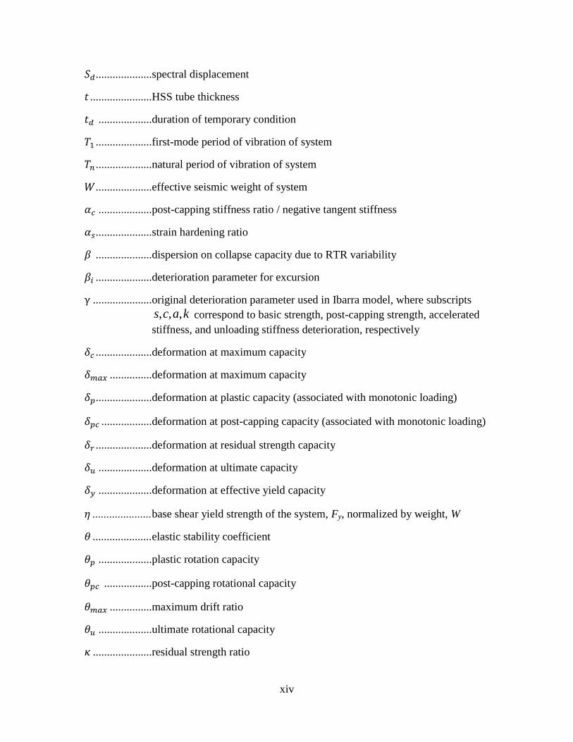
LIST OF SYMBOLS

....................specific value of an acceleration

....................random site peak horizontal acceleration

..................area of concrete

...................area of steel

......................rate of deterioration

.....................AISC coefficient used in slenderness ratio calculation

..................coefficient used in determining bond

.....................outside diameter of HSS

....................modulus of elasticity of concrete material

....................modulus of elasticity of steel material

....................hysteretic energy dissipated for excursion

....................hysteretic energy dissipation capacity

...............product of equivalent modulus of elasticity and equivalent moment of

inertia

....................uniaxial compressive strength of concrete material

....................ultimate strength of steel material

....................yield strength of steel material

( ) .............probability distribution function

....................maximum strength of system

( ) ........fragility curve at collapse capacity

..................nominal bond stress

xiii

....................residual strength of system

....................effective yield strength of system

.....................standard gravity

.....................height of system

.....................various: elastic spring stiffness, seismic load reduction factor, or a

coefficient related to the concrete mix and lateral pressure

..................post – capping stiffness of system (negative tangent stiffness)

...................effective elastic stiffness of system

...................strain hardening stiffness of system

...................unloading stiffness of system

..............length of bond region

....................mass of system

................median collapse capacity

...................maximum moment capacity of system

..................plastic moment of system

...................residual moment (strength) ratio

..................yield moment of system

.....................load applied (can refer to axial or bending load depending upon context)

....................probability of failure

..............denotes the probability of the event within the brackets

....................axial yielding load, as calculated from AISC ( )

..................annual hazard curve

P-Δ .................P-Delta (geometric nonlinearity effects)

...................nominal bond strength

...................ductility dependent strength reduction factor

....................spectral acceleration

.................spectral acceleration at collapse

xiv

....................spectral displacement

......................HSS tube thickness

...................duration of temporary condition

....................first-mode period of vibration of system

....................natural period of vibration of system

....................effective seismic weight of system

...................post-capping stiffness ratio / negative tangent stiffness

....................strain hardening ratio

....................dispersion on collapse capacity due to RTR variability

....................deterioration parameter for excursion

.....................original deterioration parameter used in Ibarra model, where subscripts

kacs ,,, correspond to basic strength, post-capping strength, accelerated

stiffness, and unloading stiffness deterioration, respectively

....................deformation at maximum capacity

...............deformation at maximum capacity

....................deformation at plastic capacity (associated with monotonic loading)

..................deformation at post-capping capacity (associated with monotonic loading)

....................deformation at residual strength capacity

...................deformation at ultimate capacity

...................deformation at effective yield capacity

base shear yield strength of the system, Fy, normalized by weight, W

.....................elastic stability coefficient

...................plastic rotation capacity

.................post-capping rotational capacity

...............maximum drift ratio

...................ultimate rotational capacity

.....................residual strength ratio

xv

.....................various: modified deterioration parameter (same subscripts used as for ),

a scale factor used in IDAs, slenderness ratio, mean

..................mean annual frequency of collapse

..............slenderness ratio of CCFT

................slenderness ratio of HSS

.................mean hazard curve

.....................deterioration parameter implemented in OpenSees (same subscripts used

as for )

.....................damping ratio of system

..............standard deviation of the log of the collapse capacity

LIST OF ABBREVIATIONS

AASHTO .......The American Association of State Highway and Transportation Officials

ABC ...............Accelerated Bridge Construction

ACI .................The American Concrete Institute

AISC ..............The American Institute of Steel Construction

ASCE .............The American Society of Civil Engineers

ASTM ............The American Society for Testing and Materials

Caltrans ..........The California Department of Transportation

CCFT..............Circular Concrete Filled (steel) Tube (nomenclature used in this research)

CFST ..............Concrete Filled Steel Tube (nomenclature used in other research reviewed

herein)

CFT ................Concrete Filled (steel) Tube (can include circular, square or rectangular

sections)

DBE................Design Basis Earthquake

DBSL .............Design Basis Seismic Load

DM .................Damage Measure

DOF................Degree of Freedom

DOT ...............Department of Transportation

EDP ................Engineering Demand Parameter

FC ...................Fragility Curve

FEA ................Finite Element Analysis

FEMA ............The Federal Emergency Management Agency

GM .................Ground Motion

xvii

HC ..................Hazard Curve

HSC ................High Strength Concrete

HSS ................Hollow Structural Section

IDA ................Incremental Dynamic Analysis

IM ...................Intensity Measure

LRFD .............Load and Resistance Factor Design

LSD ................Limit States Design

LVDT .............Low Voltage Displacement Transducer

MDOF ............Multiple Degree of Freedom

NPP ................Nuclear Power Plant

PEER ..............The Pacific Earthquake Engineering Research Center

RC ..................Reinforced Concrete

RSL ................Reduced Seismic Load

RTR ................Record to Record (variability)

SCC ................Self Consolidated Concrete

SDOF .............Single Degree of Freedom

SF ...................Safety Factor

ACKNOWLEDGEMENTS

I would like to thank everyone who provided assistance for this work. I am

particularly grateful to my advisor, Dr. Luis Ibarra, for the guidance and assistance he has

given me in furthering this research. I couldn’t have a better mentor.

I am grateful for the support of my colleagues at the University of Utah. I am

fortunate in the group of people with which I work – we learn from each other every day.

The OpenSees analytical models are extended from, and would not have been

possible without, the work of many researchers, including Frank McKenna, Silvia

Mazzoni, Dimitrios Lignos, Dimitrios Vamvatsikos, and Laura Eads.

The scope of this project being limited to analysis, the previous researchers who

have performed CCFT experiments were critical. In particular, the research of Julia

Marson and Michael Bruneau was the foundation from which the current research was

developed.

I am grateful to the University of Utah and to the Mountain-Plains Consortium for

the funding provided for this research. This material is based upon work supported by the

Mountain Plains Consortium under project MPC-404.

Finally, I would like to thank my family for their support during my graduate

studies.

INTRODUCTION

This research evaluates the seismic performance of circular concrete-filled tube

(CCFT) columns in accelerated bridge construction (ABC) projects. The objective of

ABC is to accelerate the construction schedule. For this reason, current ABC designs

usually use precast concrete columns grouted to rebar connections at base and top, if

intermediate columns are required. The bridge can be assembled in a few days, but the

seismic performance objectives cannot be reached until the columns’ top and base

connection grout reaches design strength. There are additional issues of concern with the

use of precast concrete intermediate columns: the precast connection is difficult to

construct because of congestion at the connection splices and potential rebar

misalignments. Also, the use of precast columns assumes precast components are readily

available, which is not always the case, specifically in emergency bridge construction,

one of the primary applications of ABC.

Were CCFT columns instead to be used, the distinct advantage is that the

connection at the top and bottom of the column is a standard bolted connection – capable

of resisting design loads upon being bolted, without the need to wait for design strength

to be reached. The bolted connection also eliminates the issue of rebar congestion at the

connection, faced in the case of the grouted precast column connection, and the materials

– steel tubes and concrete – needed to construct CCFT columns are readily available.

The time the CCFT concrete filling takes to cure, and the column’s reduced

2

capacity for that duration, poses a primary challenge if CCFT columns are to be

considered as a viable alternative for ABC. This study investigates whether a designation

of temporary condition can be used to reduce the Design Basis Earthquake (DBE).

A design-basis bridge is selected to evaluate the seismic performance of CCFT

columns before the concrete achieves the design compressive strength. It is modeled in

OpenSees (McKenna et al., 2000) using a concentrated plasticity model. For validation of

the model, experimental data of CCFT columns subjected to static cyclic loading

(Marson, 2000) are matched with the analytical model. The model is then used for

analysis of the design-basis bridge.

Background and Motivation

Concrete-filled tubes (CFTs) are steel tubes (e.g., hollow structural sections,

HSSs), used as formwork, into which concrete is poured. CFTs have received

considerable attention in the engineering community primarily because of their high

performance under several failure modes. As compared with unfilled HSSs, CFTs have

higher axial capacity, ductility, energy absorption, and fire resistance (Zhao et al., 2010).

In addition, CFTs can be constructed using standard structural materials readily available.

This makes them ideal to use in remote geographical areas and in cases of emergency

construction where other more complex structural assemblies would be either cost or time

prohibitive. In addition, the CFT assembly is nonproprietary and is affordable in

comparison to assemblies with comparable performance.

The use of CCFT for bridge piers has gained popularity over the past several

years. An early comparison between alternatives can be seen in Figure 1. The bridge of

Figure 1c was constructed in Japan in 1982. At that time, the concrete filling was used

3

with the objective of increasing the column’s strength and expected deflection capacity.

After the Hyogoken-Nanbu earthquake of 1995, CFTs were used in bridge

construction because of their ductility. The objective was the fabrication of bridge

columns with high ratios of ductile capacity to compressive strength. As an alternative to

increasing shear reinforcing in RC columns, using CFTs in bridge construction was an

attractive option. (Kitada, 1998)

The current performance objective of highway bridge seismic design is for the

superstructure to behave elastically, while the substructure may exhibit inelastic ductile

behavior during large seismic events (AASHTO, 2012). With the need for ductile

behavior, the use of CCFT for bridge piers is gaining traction.

The list of potential advantages of CCFT for ABC includes: (i) the steel tube

provides confinement to the concrete, allowing full composite behavior to develop, which

in turn allows greater energy dissipation, (ii) the steel tube acts as formwork for the

concrete filling, (iii) the steel tube makes steel reinforcing bars unnecessary, (iv) with the

use of weathering steel or proper coatings steel tubes are weather-resistant, (v) the

concrete provides continuous buckling resistance for the steel tube, significantly

increasing ductility, and thereby the energy dissipation of the column, (vi) the concrete,

through bond with the steel, provides increased capacity through composite action.

CCFTs are selected for this study because circular cross sectional CFT are better

able to resist multiple cycles of lateral loading, remaining ductile longer than their

rectangular counterparts (Kitada, 1991, 1992). Additionally, the circular cross section

shape results in superior concrete confinement.

4

Statement of Problem

This project addresses whether it is practical to use concrete-filled steel tubular

(CFT) columns for accelerated bridge construction (ABC). Of particular issue with this

method is the time it takes for CFT columns to reach design strength relative to the time

available before the bridge must be in service. Note that the steel tube alone, assuming

the concrete only provides lateral support against buckling, is strong enough to withstand

gravity loads. The use of a reduced seismic hazard for temporary conditions can be used

to shorten the time after which the bridge can be in service.

Scope and Objectives

This study’s scope includes the review of existing literature and research related

to CCFT beam-columns, to temporary conditions, and to ABC. Using this background,

concentrated plasticity models are created that accurately reflect the behavior results from

experimental tests.

The objective of the research is to predict whether CCFT columns can be used in

ABC before the concrete reaches the full design strength, without significantly increasing

the system’s probability of failure. The study generates concentrated plasticity models to

reliably predict the nonlinear performance of CCFT components up to the collapse limit

state and calibrates for first time the deteriorating nonlinear parameters required for these

numerical simulations.

Also, a methodology for determining the probability of failure considering a

temporary condition is applied to CCFT columns. Temporary conditions are often used in

the nuclear industry, but they are applicable for CCFT columns during the first 28 days

because the temporary condition is well-defined and discrete.

5

Methodology

This research starts with determination of parameters of the plastic spring for use

in a concentrated plasticity analytical model of a CCFT column. These are calibrated by

comparison with experimental CCFT hystereses, considering the effects of P-Δ. The

proposed CCFT column design is chosen on the basis of its comparable P-M envelope

with that of the RC column. Once the CCFT column is designed, and the plastic spring

parameters are known, the proposed column is subjected to monotonic, static cyclic,

single dynamic loading, and incremental dynamic analyses (IDAs), as a function of

concrete age, using a concentrated plasticity model.

The IDAs are performed using 44 far-field ground motions. The failure mode

mechanism to be evaluated is the collapse limit state, which can be obtained for the

selected CCFT column under dynamic loading for different concrete strengths (3, 7, 14,

and 28 days). Fragility curves are developed from the IDAs. A hazard curve is created for

Salt Lake City, Utah using a reduced design basis earthquake as a function of the time the

concrete core in the CCFT has been allowed to cure. Ultimately, the fragility curves and

the hazard curve are numerically integrated to obtain the probability of failure for

different concrete strength conditions.

6

(a)

(b)

(c)

Figure 1 Bridge Piers: a) Steel, b) CFT, c) CCFT.

Reprinted from Kitada, T., Ultimate Strength and Ductility of State-of-the-Art Concrete-

Filled Steel Bridge Piers in Japan. Engineering Structures 1998, 20 (4), 347-354,

Copyright (1998), with permission from Elsevier.

LITERATURE REVIEW

This section is divided into i) CFT behavior under seismic loading, ii) CFT

concrete strength as a function of time, and iii) temporary conditions.

Seismic Behavior of Concrete Filled Steel Tube Columns

The concrete core of CFT has two functions: to increase flexural stiffness and

ultimate strength, and to prevent local buckling of the steel tube. Whereas a slender HSS

is usually limited by buckling failure, the increase in CFT capacity is caused by the added

compression strength from the presence of concrete in CFTs, which also provides

continuous bracing for the steel tube (Zhao et al., 2010).

Local buckling of a CFT column is significantly reduced from that of an unfilled

steel tube column, but it is not eliminated completely. Local buckling mainly depends on

the ratio of the outside diameter of the steel tube to its thickness ( ratio). Concrete

filling increases the buckling threshold as much as 70% (Zhao et al., 2010). CCFT

columns are selected for this study because they can resist bending forces equally well

from any direction due to non-directionality of their circular cross section. CFT columns

also have a high strength-to-weight ratio due to confinement of concrete.

8

Slenderness Ratio

The slenderness ratio for CCFT is defined by AISC (AISC, 2010b) as a function

of the type of loading applied and as compared to the same diameter HSS. For the HSS,

the slenderness ratio is

( 1 )

where is the outer diameter of the steel and is the thickness of the steel tube.

The CCFT slenderness ratio is defined as

( 2 )

where is the modulus of elasticity of the steel

is yielding strength of steel and

is an empirical coefficient defined by AISC, varying between 0.09 and 0.31

depends on whether axial or bending loading is applied and the CCFT

slenderness ratio.

The design equations governing the design of the CCFT are determined

depending upon how the CCFT slenderness ratio compares to that of the HSS of the

equal diameter.

An et al. (2012) investigated the behavior and failure modes resulting from axial

compression of slender and thin-walled CCFT columns. They found CCFT columns

under axial compression exhibit elastic and elastic-plastic instability failure. They also

concluded that the failure mode of very slender circular CCFT columns is elastic

instability, and concrete strength is less relevant in slender CCFT columns. They

9

confirmed that the ultimate strength is determined by the column’s flexural rigidity, is

inversely related to slenderness ratio, and directly related to steel ratio and concrete

strength. Han et al. (2011) also tested CFT columns under cyclic loading, concluding

that column bending and shear capacity are the main failure mechanisms, whereas

buckling is usually prevented by the continuous lateral support of the concrete.

Concrete Confinement

The axial and flexural strength of a CFT column is greater than that of either an

equivalent concrete column or of an unfilled steel tube column, due to concrete’s

tendency to have a higher Poisson ratio than steel at high loads (Ranzi et al., 2013). That

is, the steel tube confines the concrete and prevents transverse expansion of the concrete.

As the stresses in the column increase, the concrete transverse expansion amount

increases, and the confinement effect provided by the steel is magnified. This

confinement then serves to equivalently increase the axial strength of CFT columns,

particularly for shorter columns.

Knowles and Park (1969) investigated the effect of slenderness ratio on axial

strength of CFT columns and found that slenderness ratio plays a role in concrete

confinement. They concluded for a slenderness ratio of less than 35, concrete

confinement is ensured.

Composite Action

Composite action allows CFT columns to resist buckling, have good ductility, and

high axial resistance. Composite action relies upon bond behavior at the steel-concrete

interface, which according to AISC (2010b), can be estimated as:

10

( 3 )

where:

is nominal bond strength, in kips

is the outside diameter of the HSS, in in.

= 2 if the filled composite member extends to one side of the point of force

transfer, or 4 if the filled composite member extends on both sides of the point

of force transfer

is nomimal bond stress = 0.06 ksi

and for LRFD, = 0.45.

This formula incorporates the two types of bond transfer: circumferential,

, and longitudinal, . The bond stress value is a lower bound adopted from

experimental data. Some experimental tests have shown, however, that the entire

circumference can contribute to circumferential bond (Zhang et al., 2012).

Zhang et al. proposed new formulas, based upon finding a correlation between

bond behavior and the cross-sectional dimensions of the CFT, and extant experimental

data from push-out, push-off, and connection tests. They posited that transfer length,

dictating longitudinal bond behavior, varies according to material and geometric

properties, and can increase axial load capacity. The transfer length used in design

calculations must address two limit states: slip along the entire length of the column and

local slip near the point of load application.

Experimental results show that in the case of a column with at least two girders

framing into opposite sides, bond stresses are developed around the entire perimeter

(Zhang et al., 2012). They also found that it is justified to use the entire circumference as

11

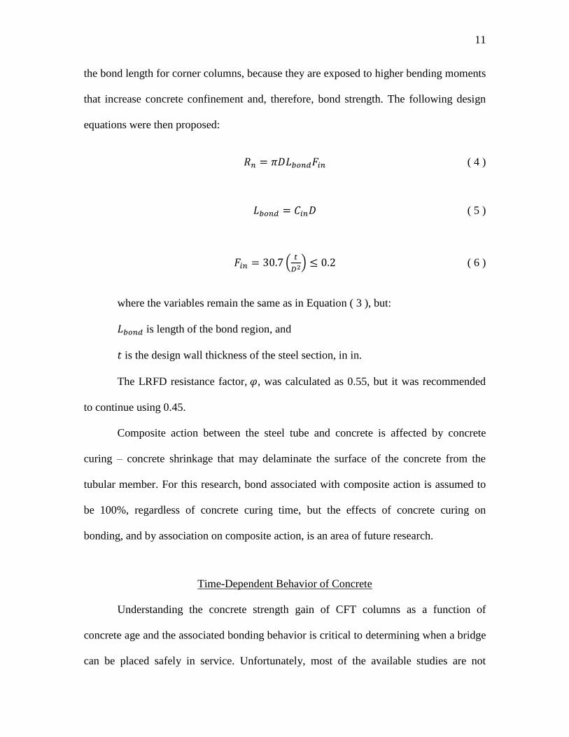
the bond length for corner columns, because they are exposed to higher bending moments

that increase concrete confinement and, therefore, bond strength. The following design

equations were then proposed:

( 4 )

( 5 )

(

) ( 6 )

where the variables remain the same as in Equation ( 3 ), but:

is length of the bond region, and

is the design wall thickness of the steel section, in in.

The LRFD resistance factor, , was calculated as 0.55, but it was recommended

to continue using 0.45.

Composite action between the steel tube and concrete is affected by concrete

curing – concrete shrinkage that may delaminate the surface of the concrete from the

tubular member. For this research, bond associated with composite action is assumed to

be 100%, regardless of concrete curing time, but the effects of concrete curing on

bonding, and by association on composite action, is an area of future research.

Time-Dependent Behavior of Concrete

Understanding the concrete strength gain of CFT columns as a function of

concrete age and the associated bonding behavior is critical to determining when a bridge

can be placed safely in service. Unfortunately, most of the available studies are not

12

focused on the short time period during which concrete strength gain is attained, but

longer term measurements.

Because concrete is pumped into the steel tubes, its exposure to air is minimal,

affecting its ability to dry as part of the curing process. This sealed condition may affect

creep and shrinkage processes. Using creep coefficients ranging from 50-60% of the

typically recommended values conservatively predicts experimental findings (Ranzi et

al., 2013). For this research, creep is not of central concern due to creep being a long-

term process, and is not expected to affect column behavior during the first 28 days.

For typical concrete mixes, drying shrinkage is significantly different for CCFT

from typical concrete exposed to air, while autogenously shrinkage is not affected by the

lack of exposure to air. Experiments were conducted on CCFT specimens allowed to cure

long-term, unloaded. The amount of shrinkage measured was very small, and some

studies have suggested shrinkage may be neglected for CCFT (Ranzi et al., 2013).

Creep and shrinkage result in stress redistribution at the interface between the

steel tube and the concrete filling. Usually perfect bond / composite behavior is assumed

between the steel and concrete. Then full shear interaction theory can be applied in

analysis of the column, showing good agreement with experimental results of long-term

measurements. The effect of creep on ultimate axial strength of CCFT is not clear. Some

researchers found that creep reduces the carrying capacity for up to 20%, whereas others

found that creep has no effect (Ranzi et al., 2013).

The effect of concrete confinement in CCFT is increased further by the low level

of shrinkage exhibited by CCFT. However, experimental findings may over predict

confinement because the loading is commonly applied to the concrete, not the steel or the

13

entire composite section (Ranzi et al., 2013).

Temporary Conditions

Temporary conditions will be investigated for use in the period of time before the

concrete has achieved full design strength. In the case of ABC projects, reducing curing

time through use of concrete accelerating admixtures could be disadvantageous.

One of the most common accelerating admixtures used is calcium chloride

(CaCl2). In addition to accelerating strength gain, it increases drying shrinkage and steel

corrosion (Kosmatka and Panarese, 2002), both of which pose problems for CCFT.

Drying shrinkage reduces bond strength and composite action, and thereby, ductile

behavior. Due to concrete in CCFT being encapsulated from air, drying shrinkage will

not be as significant as in other types of construction, but no studies have been done to

quantify the effects of drying shrinkage. Steel corrosion, likewise, can affect the external

tube surface, and more critically, the interior of the tube, where it can be potentially

undetected. The alternative to accelerating strength gain is to address the performance of

CFT columns under gravitational and seismic loading before conventional concrete

reaches its design strength, and consider the seismic hazard risk reduction due to this

temporary condition.

Cornell and Bandyopadhyay (1996) evaluated several scenarios in which nuclear

facilities might have reduced seismic design loads. The methods for determining reduced

seismic loads fall into categories of intermittent load combinations, probability of failure

argument, and the risk averaging argument.

Temporary conditions are currently used in nuclear facilities, but there is

ambiguity about what constitutes a temporary condition (Hill, 2004). By contrast,

14

temporary conditions for CFT within ABC are well-defined, having an upper limit for the

temporary condition designation: after the concrete reaches its design strength, the

temporary condition is discarded. Temporary conditions can be considered by applying a

reduced seismic load (RSL) during the duration of the temporary condition.

Reduced hazard levels for temporary conditions have been investigated for

several loading conditions. Boggs and Peterka (1992) created a model to represent the

probability of a wind speed resulting in structural failure of a temporary structure. They

derived a correlation between the design recurrence interval of a permanent structure and

that of a temporary one. The correlation was derived by first evaluating the failure

probability of permanent structures due to high wind speed. The probability of failure

was defined in terms of the probability of a wind speed exceeding that wind speed whose

magnitude resulted in structural failure.

To obtain adequate safety for temporary conditions, Boggs and Peterka (1992)

indicated that either the safety factor, SF, must be increased, or the mean recurrence

interval of the design wind speed for temporary structures must be increased. The study

mentions that the methodology presented is imprecise and not a good predictor of

recurrence interval for increasingly short periods of less than a year. This issue is relevant

for CCFT in ABC, in which temporary conditions would be of significantly shorter

duration than a year.

In response to the paper by Boggs and Peterka, Hill (2004) questioned the logic

and safety of allowing reductions in design load due to conditions that are evaluated as

temporary, but may be permanent loading conditions. Hill acquiesced there are legitimate

temporary conditions which can benefit from design load reductions during the duration

15

of the temporary condition. This is the case in CCFT construction, which has a defined

upper limit for the temporary condition designation. After the concrete reaches the design

strength, the temporary condition is discarded. In the situation of civil bridge

construction, the design strength should be assumed, in the most general case, to take 28

days to reach. In the case of ABC projects, when accelerated construction is the primary

desired objective, the 28 days become a significantly long period of time.

Amin et al. (Amin and Jacques, 1994, Olson et al., 1994) evaluated seismic

loading for temporary conditions in nuclear power plants. They used annual seismic

hazard curves to determine acceleration levels corresponding to temporary loads in which

the corresponding acceleration is dependent upon the duration of the temporary loading.

They reduced the mean annual hazard curve at the site to account for a temporary

condition. In this approach, the probability of exceedance in the hazard curve is reduced

by a linear proportion based on the temporary condition duration.

Starting with seismic acceleration at the site having a probability distribution

function of:

( ) ( 7 )

where

is the random site peak horizontal acceleration

is the specific value of an acceleration

( ) is the probability distribution function

and denotes the probability of the event within the brackets – in this case the

probability that any particular event a will exceed the peak value A.

Amin et al. then concluded that:

16

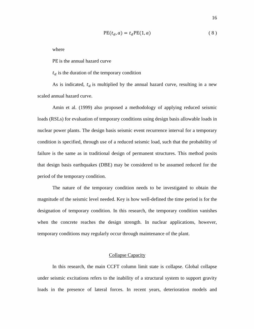
( ) ( ) ( 8 )

where

is the annual hazard curve

is the duration of the temporary condition

As is indicated, is multiplied by the annual hazard curve, resulting in a new

scaled annual hazard curve.

Amin et al. (1999) also proposed a methodology of applying reduced seismic

loads (RSLs) for evaluation of temporary conditions using design basis allowable loads in

nuclear power plants. The design basis seismic event recurrence interval for a temporary

condition is specified, through use of a reduced seismic load, such that the probability of

failure is the same as in traditional design of permanent structures. This method posits

that design basis earthquakes (DBE) may be considered to be assumed reduced for the

period of the temporary condition.

The nature of the temporary condition needs to be investigated to obtain the

magnitude of the seismic level needed. Key is how well-defined the time period is for the

designation of temporary condition. In this research, the temporary condition vanishes

when the concrete reaches the design strength. In nuclear applications, however,

temporary conditions may regularly occur through maintenance of the plant.

Collapse Capacity

In this research, the main CCFT column limit state is collapse. Global collapse

under seismic excitations refers to the inability of a structural system to support gravity

loads in the presence of lateral forces. In recent years, deterioration models and

17

experiments have been used to evaluate structural collapse (Ibarra and Krawinkler, 2005,

Lignos and Krawinkler, 2012, Villaverde, 2007) considering record-to-record (RTR)

variability as the only source of uncertainty affecting the variance of the structural

response.

A limited number of studies have evaluated the effect of uncertainty in the

modeling parameters on collapse capacity for single degree of freedom (SDOF) systems

(Ibarra and Krawinkler, 2005, Liel et al., 2009). The level of uncertainty of modeling

parameters can be large because of their intrinsic aleatory variability and especially the

inability to accurately evaluate them (i.e., epistemic uncertainty).

For modeling collapse capacity of CCFT, the evaluation should be based on

structural analyses that incorporate deterioration characteristics of structural components

subjected to cyclic loading and the inclusion of geometric nonlinearities (P- effects).

For SDOF systems, P- effects are usually included by rotating the backbone curve based

on a parameter known as the elastic stability coefficient, (Adam et al., 2004, Bernal,

1987, Jennings and Husid, 1968, MacRae, 1994, Sun et al., 1973, Vian and Bruneau,

2001).

The development of hysteretic models that include strength and stiffness

deterioration (Ibarra et al., 2005, Sivaselvan and Reinhorn, 2000, Song and Pincheira,

2000) improved the assessment of collapse capacity. Collapse of SDOF systems is

assumed to occur when the loading path is on the backbone curve and the restoring force

approaches zero. Thus, collapse requires the presence of a backbone curve branch with

negative slope, a condition caused by P- effects and/or a negative tangent stiffness

branch of the hysteresis model. Collapse capacity can be expressed in terms of a relative

18

intensity ( ⁄ ) ⁄ , where is the 5% damped spectral acceleration at the elastic period

of the SDOF system (without P- effects), and ⁄ is the base shear yield strength

of the system, , normalized by weight, . In this study, however, the structural system

is defined, and the intensity measure (IM) is the spectral acceleration at the first period of

the system, ( ) . IM is a ground motion parameter that can be monotonically scaled

by a nonnegative scalar (Vamvatsikos and Cornell, 2002).

Nonlinear time history analyses are conducted for increasing ( ) values

until the system response becomes unstable. This approach is named Incremental

Dynamic Analysis (IDA) (Vamvatsikos and Cornell, 2002). Using IDAs, collapse can be

visualized by plotting the intensity measure against an engineering demand parameter

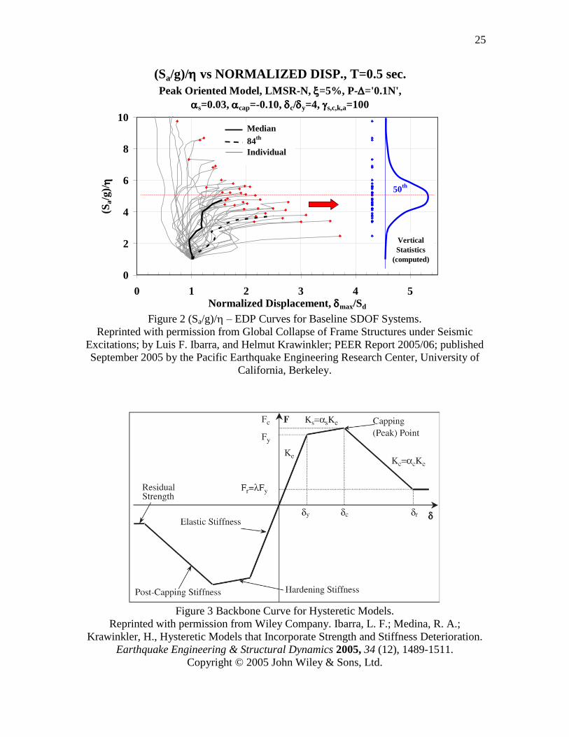
(EDP) of interest. For instance, Figure 2 presents individual and statistical relative

intensity-normalized displacement curves, ( ⁄ ) ⁄ vs ⁄ .

The deterioration characteristics of the system cause the individual curves to

eventually approach a zero slope as ( ⁄ ) ⁄ increases. The last point of each individual

curve represents the system “collapse capacity,” ( ⁄ ) ⁄ . The U.S. Federal

Emergency Management Agency (FEMA) adopted IDA as the method of choice for

determining collapse capacity (ATC, 2000a, b).

Scaling of the Ground Motion Records

The most common IM is 5-percent damped spectral acceleration at the structure’s

fundamental period of vibration, ( ) . To account for RTR variability, the 44

ground motion (GM) records from FEMA P695 (ATC, 2009) were used in this study.

Because the IM is ( ) , the records were scaled at the of the first period of the

19

system:

⁄

⁄ ( 9 )

where

is ( )

is standard gravity

is the yielding strength of system, and

is the effective seismic weight of the system.

Hysteretic Models

The CCFT columns of this study need to be represented with hysteretic models

that account for strength and stiffness deterioration. Sivaselvan and Reinhorn (2000)

developed a smooth hysteretic model which allows for deterioration in both strength and

stiffness and provides for pinching behavior, but it does not include a negative backbone

tangent stiffness. Song and Pincheira (2000) proposed a model based upon energy

dissipated. This model represents both cyclic strength and stiffness deterioration and its

back bone curve has a post-capping negative tangent stiffness and a residual strength

branch. However, the backbone curve cannot account for strength deterioration prior to

reaching peak strength. This study utilizes the hysteretic models developed by Ibarra et

al. (2005), which include four deterioration modes: basic strength, post-capping strength,

unloading stiffness, and accelerated reloading stiffness deterioration. Ibarra et al. (2005)

developed bilinear, peak-oriented, and pinching models, but only peak-oriented models

are used in this study.

20

Backbone Curve Model

The backbone curve, shown in Figures 3 and 4, defines the deformation response

for a loading protocol which increases monotonically until collapse. If there is no

deterioration, it consists of an elastic stiffness , a yield strength , and a strain

hardening stiffness . If deterioration is considered, the curve continues along the slope

of until reaching the strength at which the strain hardening interval is capped at a

maximum strength . The negative tangent stiffness (also called post-

capping stiffness) continues until the residual strength, , is reached – if one is specified.

The displacement associated with the peak strength is normalized as ⁄ , and may be

viewed as a monotonic “ductility capacity.”

The effect of P- is to rotate the backbone curve in accordance with the elastic

stability coefficient, . Figure 4 illustrates the backbone curve of this model with and

without the effect of P-.

( 10 )

where is the seismic weight of the system, and is the height of the system.

Peak-Oriented Hysteretic Deterioration Model

The peak-oriented model used in this study to represent nonlinear CFT behavior

(Ibarra et al., 2005) has the same rules of the peak-oriented model proposed by Clough

and Johnston (1966). The deterioration of the reloading stiffness for a peak-oriented

model occurs once the horizontal axis is reached (points 3 and 7 in Figure 5), and the

reloading path targets the previous maximum displacement. The model proposed by

21

Ibarra et al. (2005) can also account for residual strength.

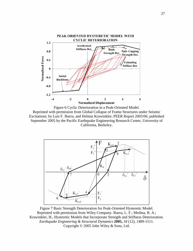
The hysteretic model includes four modes of cyclic deterioration based on energy

dissipation. As observed in Figures 6 and 7, basic strength and post-capping strength

deterioration effects translate the strain hardening and post-capping branch toward the

origin, unloading stiffness deterioration decreases the unloading stiffness, and reloading

(accelerated) stiffness deterioration increases the target maximum displacement.

As is illustrated in Figure 7, strength deterioration occurs between points 3 and 4

as a function of the basic strength deterioration rule, which affects a system prior to it

reaching its capping stiffness.

The amount of deterioration depends on the parameter , which may be different

for each cyclic deterioration mode. For instance, the unloading stiffness in the

excursion ( ) is deteriorated as:

( ) ( 11 )

where , is the deterioration parameter for unloading stiffness in the excursion. In

its general form, is expressed as:

(

∑

)

( 12 )

where is hysteretic energy dissipated in excursion , ∑ is hysteretic energy

dissipated in previous positive and negative excursions,

( 13 )

is the reference hysteretic energy dissipation capacity of component in the original Ibarra-

22

Krawinkler model (Ibarra et al., 2005).

The parameter for each deterioration mode is calibrated from experimental

results. Reasonable results are obtained if all cyclic deterioration modes are represented

by a single parameter , where the subscripts correspond to basic strength,

post-capping strength, accelerated stiffness, and unloading stiffness deterioration,

respectively.

The parameter is 1 for this study, implying a constant rate of deterioration. The

yield deformation is , is cap deformation (deformation associated with

for monotonic loading, used in the Ibarra-Krawinkler model), and is plastic

deformation capacity (used in the Lignos-Krawinkler model, discussed below).

Modified Hysteretic Model

A modified version of the deteriorating hysteretic model (Lignos and Krawinkler,

2012) developed by Ibarra et al. (2005) is implemented in OpenSees (McKenna et al.,

2000) to account for nonlinear rotational behavior (refered to in this paper as Lignos-

Krawinkler model). Where equation ( 13 ) is used for the Ibarra et al. model,

( 14 )

is the reference hysteretic energy dissipation capacity of component in the Lignos-

Krawinkler model (Lignos and Krawinkler, 2012). The central difference is in the

parameters or used instead of , to account for the underlying difference between

and where as illustrated in Figure 8 and Figure 9. As in the Ibarra et al.

model, where the parameter is assigned subscripts to represent types of strength

23

deterioration, for the OpenSees model used in this research the parameters representative

of the respective strength deterioration types are:

, basic strength deterioration

, post-capping strength deterioration

, accelerated strength deterioration

, unloading strength deterioration

This modified peak-oriented hysteretic model (Figure 8) is used to model the

equivalent stiffness as a spring in the concentrated plasticity model within OpenSees.

Cyclic Deterioration Parameter Values

Ibarra et al. and Lignos and Krawinkler matched their cyclic deterioration

parameters to experimental data to determine the reasonable range of numerical values

for cyclic deterioration parameters (Ibarra and Krawinkler, 2005, Lignos and Krawinkler,

2012).

For the Ibarra et al. model,

a) no cyclic deterioration:

b) slow cyclic deterioration: and

c) medium cyclic deterioration: and

d) rapid cyclic deterioration: and

Steel can be modeled with and RC modeled with .

Lignos proposed equations from results of a parameter study to determine ranges

of numerical values. His study looked at a great number of samples, and based on these

results, for HSS one can assume values around 0.3 correspond to rapid

24

deterioration and around 2.8 correspond to slow deterioration. Likewise, for W sections,

values around 0.8 correspond to rapid deterioration and around 3 correspond to slow

deterioration. For RC, values around 0.5 correspond to rapid deterioration and around 3

correspond to slow deterioration (Lignos and Krawinkler, 2011, 2012).

25

Figure 2 (Sa/g)/– EDP Curves for Baseline SDOF Systems.

Reprinted with permission from Global Collapse of Frame Structures under Seismic

Excitations; by Luis F. Ibarra, and Helmut Krawinkler; PEER Report 2005/06; published

September 2005 by the Pacific Earthquake Engineering Research Center, University of

California, Berkeley.

Figure 3 Backbone Curve for Hysteretic Models.

Reprinted with permission from Wiley Company. Ibarra, L. F.; Medina, R. A.;

Krawinkler, H., Hysteretic Models that Incorporate Strength and Stiffness Deterioration.

Earthquake Engineering & Structural Dynamics 2005, 34 (12), 1489-1511.

Copyright © 2005 John Wiley & Sons, Ltd.

(Sa/g)/ vs NORMALIZED DISP., T=0.5 sec.

Peak Oriented Model, LMSR-N, x=5%, P-='0.1N',

as=0.03, acap=-0.10, dc/dy=4, gs,c,k,a=100

0

2

4

6

8

10

0 1 2 3 4 5

Normalized Displacement, dmax/Sd

(Sa/g

)/

Median

84th

Individual

50th

Vertical

Statistics

(computed)

26

Figure 4 Backbone Curves for Hysteretic Models with and without P-





Figure 5 Peak-Oriented Hysteretic Model.





27

Figure 6 Cyclic Deterioration in a Peak-Oriented Model.





Figure 7 Basic Strength Deterioration for Peak-Oriented Hysteretic Model.





28

Figure 8 Parameters for Peak-Oriented Hysteretic Lignos-Krawinkler Model.

Adapted from Lignos, D. G. Modified Ibarra-Medina-Krawinkler Deterioration Model

with Peak-Oriented Hysteretic Response (ModIMK Peak Oriented Material).

http://opensees.berkeley.edu/wiki/index.php/Modified_Ibarra-Medina-

Krawinkler_Deterioration_Model_with_Peak-

Oriented_Hysteretic_Response_(ModIMKPeakOriented_Material).

Copyright (1999, 2000) The Regents of the University of California. All rights reserved.

29

Figure 9 Parameters for Backbone Curve for Lignos-Krawinkler Model.

Reprinted with permission from Lignos, D. G.; Krawinkler, H., Sidesway Collapse of

Deteriorating Structural Systems Under Seismic Excitations. In The John A. Blume

Earthquake Engineering Center, Stanford University: 2012.

ANALYSIS OF EXPERIMENTAL CIRCULAR CONCRETE

FILLED STEEL TUBE COLUMNS

There are extensive experimental databases for CCFT. However, cyclic loading

experimental data of normal strength CCFT of appropriate dimensions and boundary

conditions for highway bridges are scarce.

Among the most recent well-compiled experimental databases for CCFT are those

from Goode (2013) and Leon et al. (2011). However, the available database is quite

limited for a specimen possessing bridge column characteristics, such as: normal strength

circular steel tube, normal strength concrete filling, relatively large ratio, fixed base

condition, and constant axial load of appropriate value. The experimental data with

the specimens most closely applicable to the determination of highway bridge parameters

included the three experiments described below.

Boyd et al. (1995) performed static cyclic tests on five CCFT with constant axial

load. The columns had a diameter of 203.2 mm, and relatively large ratios of either

106 or 73. The researchers concluded that the steel tube thickness and the addition of

steel studs increased energy dissipation. The steel studs reduced deterioration at large

deformations. These specimens, however, included HSC that resulted in less ductility,

greater degradation, and less energy dissipation than normal strength concrete.

Elremaily and Azizinamini (2002) performed tests which were closely related to

31

the current research in terms of ratios and loading protocol, but with the parameters

they wanted to consider (high strength concrete, and various ⁄ ratios), only one of

their specimens could have been used in this study.

The tests from Marson and Bruneau (2004) were selected for this research

because they include the main characteristics of CCFT bridge columns. Marson and

Bruneau (2004) tested four columns (CFST64, CFST51, CFST34, and CFST42) under

static cyclic loading protocols. These specimens have characteristics expected in highway

bridges, such as relatively large ratios, fixed base condition, normal strength

concrete, and constant axial load of appropriate values. They performed inelastic

static cyclic tests until rupture of the steel tube, all of which reached 7% drift prior to

rupture.

They determined the specimen sizes after compiling parameters from more than

1200 highway bridges. The digits at the end of CFST64, CFST51, CFST34, and CFST42

refer to the nominal , which differs from the measured . Slenderness ratios of

less than 35 were selected based on the research of Knowles and Park (1969), and

ratios were also based on the bridge database.

The tested specimens showed local buckling at about , which

coincided with the highest applied lateral force. Hysteretic pinching behavior was

observed in CFST64; its larger ⁄ ratio is indicative of a larger contribution to behavior

from concrete, which is best represented as between a peak-oriented and pinching

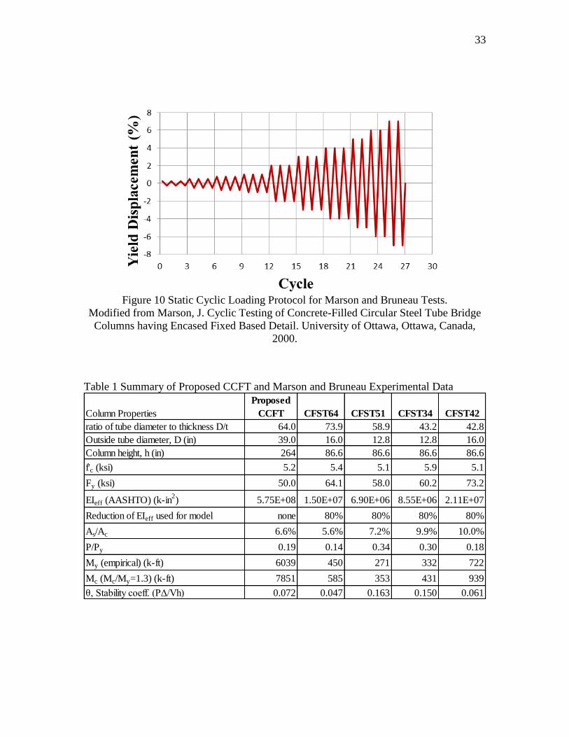
hysteretic model. The tests were stopped at a cycle of , where necking of steel tube

and significant concrete cracking was observed (Marson and Bruneau, 2004). The cyclic

loading protocol is shown in Figure 10.

32

The tested specimens showed local buckling at about , which

coincided with the highest applied lateral force. Hysteretic pinching behavior was

observed in CFST64; its larger ⁄ ratio is indicative of a larger contribution to behavior

from concrete, which is best represented as between a peak-oriented and pinching

hysteretic model. The tests were stopped at a cycle of , where necking of steel tube

and significant concrete cracking was observed (Marson and Bruneau, 2004).

The columns were opened after the testing. The concrete in the columns’ base was

pulverized, but was intact at the upper face of the foundation. The researchers indicated

that the concrete directly below and above the buckled area remained intact, which shows

that concentrated plasticity models should provide a reasonable numerical approximation.

Hysteretic degradation parameters have been derived for steel and RC components, but

the parameterization did not exist for CCFT columns. The degradation parameters were

determined by curve-fitting the OpenSees analytical concentrated plasticity model with

the Marson and Bruneau experimental data. A data summary of these experimental

columns is shown in Table 1 (see Appendix A for the rest of the data). Note that Table 1

also presents the proposed CCFT column data based on the column design described in

the next section.

33

Figure 10 Static Cyclic Loading Protocol for Marson and Bruneau Tests.

Modified from Marson, J. Cyclic Testing of Concrete-Filled Circular Steel Tube Bridge

Columns having Encased Fixed Based Detail. University of Ottawa, Ottawa, Canada,

2000.

Table 1 Summary of Proposed CCFT and Marson and Bruneau Experimental Data

Column Properties

Proposed

CCFT CFST64 CFST51 CFST34 CFST42

ratio of tube diameter to thickness D/t 64.0 73.9 58.9 43.2 42.8

Outside tube diameter, D (in) 39.0 16.0 12.8 12.8 16.0

Column height, h (in) 264 86.6 86.6 86.6 86.6

f'c (ksi) 5.2 5.4 5.1 5.9 5.1

Fy (ksi) 50.0 64.1 58.0 60.2 73.2

EIeff (AASHTO) (k-in2) 5.75E+08 1.50E+07 6.90E+06 8.55E+06 2.11E+07

Reduction of EIeff used for model none 80% 80% 80% 80%

As/Ac 6.6% 5.6% 7.2% 9.9% 10.0%

P/Py 0.19 0.14 0.34 0.30 0.18

My (empirical) (k-ft) 6039 450 271 332 722

Mc (Mc/My=1.3) (k-ft) 7851 585 353 431 939

θ, Stability coeff. (PΔ/Vh) 0.072 0.047 0.163 0.150 0.061

DESIGN OF A CIRCULAR CONCRETE FILLED STEEL TUBE

COLUMN

A Caltrans bridge was selected for this research from a set of benchmark bridges

used in PEER studies. The original circular RC columns were replaced by CCFT columns

with similar interaction diagrams. Numerical analyses using concentrated plasticity

models were used for this evaluation. These analyses were verified through modeling of

published experimental data.

Design Basis Bridge

In 2004, PEER funded a study of seismic performance of highway bridges in

California (Ketchum et al., 2004). The researchers selected bridge types to represent the

most common highway bridge types employed by Caltrans. For this research, bridge type

1A of this study was adopted (Figure 11). The bridge consists of five straight spans with

lengths of 120, 150, 150, 150, and 120 ft. The deck consists of posttensioned cast in situ

39 ft. wide, 6 ft. deep concrete box girders to allow two 12 ft. lanes for traffic, a 4 ft. left

shoulder, an 8 ft. right shoulder, and traffic barriers at the perimeter. The single column

piers are 4 ft. diameter RC columns 22 ft. tall. The data for the design-basis bridge RC

column are shown in Table 2. A buckling analysis for the proposed CCFT according to

AISC (2010a, b) and AASHTO (2012) specifications and a buckling analysis of the RC

column according to ACI (2008) specifications is presented in Appendix B.

35

Force-Moment Interaction Diagrams

A CCFT column was designed to match the moment capacity of the original RC

column of the design basis bridge using a relatively large ratio of 64. Steel strength

was chosen using AISC’s recent adoption of ASTM A1085-13 steel specification for

HSS (Winters-Downey et al., 2013). Concrete strength was matched to that of the design

basis bridge’s RC column.

To determine the strength of the proposed CCFT column, a force-moment (P-M)

interaction diagram was created using the AISC recommended method for CCFT

(Gerschwindner, 2010). This involves using plastic section moduli of areas of steel and

concrete in radian measure for five points and linearly interpolating between the points as

needed. An interaction diagram was created for the design-basis bridge RC column using

radian measure and stress block calculations for both the concrete and the reinforcing

steel – see Appendix C for calculations and Maple script used. Additionally, for

comparison, an HSS of same diameter and tube thickness as the CCFT was included in

the interaction diagram.

The calculations used to create the CCFT interaction curve (Gerschwindner, 2010,

Leon and Hajjar, 2007, 2008) consider the combined axial and bending loads. The HSS

slenderness ratio, also referred to as the ⁄ ratio, is still of primary importance. This

method is shown in Appendix C.

Figure 12 shows a comparative interaction diagram of the CCFT used in this

study and that of the corresponding HSS. For comparison purposes, the interaction curve

for the HSS component is calculated using a radial stress block method, and AISC code

equations.

36

As observed in Figure 12, the addition of the concrete filling results in

significantly larger capacity for the CCFT, both axially and in bending, than that for the

HSS (about 50% greater peak moment capacity). Additionally, the HSS (unfilled) axial

capacity of 3,575 kips indicates that for the design basis bridge used for this study and its

corresponding gravity load of 1,822 kips, the HSS alone is capable of resisting all of the

axial load.

To obtain the equivalent CCFT column, the maximum moment capacity of the

RC column was matched using different CCFT column diameters and typical D/t ratios.

For a ratio of 64, a 39 in. outer diameter and a 0.61 in. thick steel tube resulted in the

closest fit to the peak moment capacity. Using a diameter of 38 or 40 in. would have

resulted in a more standard diameter, the differences were significant enough that a 39 in.

diameter was selected. Although not technically a HSS or Jumbo HSS as the size is too

large, it is treated as though subject to the same standards set by AISC and ASTM, and

uses concrete design strength equal to the RC column of the PEER evaluated design-basis

bridge, ksi.

Figure 13 shows the P-M interaction diagrams of the bridge RC column at full

design strength and the proposed CCFT column as a function of concrete age. The RC

column has the greater resistance axially, due in part to its larger cross-sectional area, but

the CCFT column has a larger moment resistance because of the steel tube outer

perimeter location. Another important advantage of the CCFT column is found in

comparing the moment capacity when no axial load is applied to the maximum moment

capacity. These two values (4,645 and 5,593 k-ft., respectively) indicate that without

axial load, the CCFT has 83% of its maximum moment capacity as compared to the

37

corresponding values of the RC column (3,461 and 5,591 k-ft.), equating to the RC

column having only 62% of its maximum moment capacity without axial load being

applied.

Using the largest moment capacity as a reference point, it is observed that the RC

column has a larger axial resistance because it has a greater cross section, but the CCFT

has the greater moment resistance due to the optimal location of the steel material. To

evaluate the effect of time on the strength of the proposed CCFT, full bond strength is

assumed regardless of concrete age.

Concrete gains strength as a function of time as cement is hydrated. The process

of cement hydration continues for years, but the most appreciable strength gain occurs in

the first 28 days. Determination of percentage concrete strength relative to 28-day

concrete strength as a function of time involves several assumptions. Curing conditions

such as temperature, sealed versus air curing, as well as cement type used, affect the

relative strength expected at any given time. Experimental reported values for relative

strength gain as a function of time vary (Mindess et al., 2003), but in general, concrete at

28 days is on average 1.5 times stronger than at 7 days (but this value varies between 1.3

and 1.7) (Hassoun and Al-Manaseer, 2012).

For this research, 28 days being considered as full strength (or as a value of 1),

14, 7, and 3 days were considered as 0.90, 0.65, and 0.40, respectively. The gain in

concrete strength as a function of time is shown in Figure 14 a. Figure 14 b. uses the data

of the P-M diagram of Figure 13 to show the relative capacity of the CCFT column as a

function of concrete age as a percentage of the design (at 28 days). The results are

presented for the conditions of pure axial load, pure bending moment, and maximum

38

moment capacity. As observed, the moment capacity of the column is less dependent on

time than the axial capacity because the largest contribution to moment capacity is

provided by the steel tube.

The yield moment of the CCFT specimens, , is determined by inspection of the

hysteretic curves (lacking experimental pushover curve data) and compared with the

plastic moment of the specimens, , as calculated using AISC P-M diagrams. The

resulting ratio of experimental to values is averaged and used to determine the

predicted value of for the proposed column. Similarly, from inspection of

experimental hysteretic curves, a ratio of to , or the ratio of maximum moment

capacity to yield moment capacity, is determined and verified through curve-fitting the

analytical hysteretic model to experimental hystereses. This ratio is then used to

predict values for the proposed CCFT as a function of concrete age. Table 3

summarizes the data for the proposed CCFT – see Appendix A for full data. The number

at the end of the CCFT acronym refers to the curing time.

Analytical Model

Experimental tests show that CCFT nonlinear performance can be reasonably

predicted using concentrated plasticity models. Marson and Bruneau found, for instance,

localized rupture of the steel tube and pulverized concrete slightly above the fixed base.

A concentrated plasticity model was thereby created in the program OpenSees using the

Ibarra et al. peak-oriented hysteretic model (Ibarra et al., 2005, Lignos, 2012).

The column is modeled with an elastic beam-column element, meaning that all

inelastic, or plastic deformation is accounted for in the spring at the base. This zero

39

length spring represents a deteriorating peak-oriented hysteretic model (Ibarra et al.,

2005, Lignos and Krawinkler, 2012). The OpenSees script allowed for monotonic

loading, static cyclic loading using Marson and Bruneau’s loading protocol, single

dynamic record loading, and IDA. The analysis options could include or disregard P-

effects to isolate geometric from material nonlinearity. The gravity load lumped at the top

node of the elastic beam-column element includes the dead load, as calculated from the

superstructure self-weight for the tributary area of the design-basis bridge, as well as the

self-weight of the column.

Because all plastic deformation is accounted for in the concentrated hinge

location, and the elastic beam-column element has no dimensional width, the elastic

beam-column input only needs to have a few definitions provided:

, the product of equivalent modulus of elasticity and equivalent

moment of inertia;

, the column height;

, the concentrated mass;

, the applied horizontal force;

, the yield moment capacity; and

⁄ , the maximum moment capacity to yield moment capacity ratio.

Deterioration Parameters

Deteriorating hysteretic parameters were determined from the experimental data

of Marson and Bruneau (2004). These parameters are in large part a function of the

stability coefficient, , ratio of steel tube diameter to thickness, , and ratio of area of

40

steel to concrete, ⁄ . The analytical model accounts for deterioration due to material

nonlinearity and P- effects (geometric nonlinearity). The main parameters used in

curve-fitting the analytical model to the experimental columns included a plastic rotation

capacity 0.08, a post-capping rotational capacity 0.10, basic strength

deterioration = 4.0, and accelerated reloading stiffness deterioration = 1.6. Note

that the value for basic strength deterioration compares favorably with Lignos’ finding

that = 3.0 (or greater) indicates slow cyclic deterioration, with steel and concrete beam

columns with good cyclic performance having = 3.0. Therefore, = 4.0 is indicative

of CCFT behaving better under cyclic loading than either steel or concrete alone, which

is in agreement with previous studies in which CCFT specimens exhibited higher axial

and bending strength than either steel or concrete beam-columns (Ranzi et al., 2013).

Table 4 shows the values for the cyclic deterioration determined appropriate for

the experimental CCFT specimens. These results are used to select the backbone curve

properties and cyclic deterioration parameters for the proposed CCFT column model.

Graphic representation of parameters can be seen in Figure 8.

Based on previous parameter studies (Ibarra and Krawinkler, 2005, Lignos and

Krawinkler, 2012), a basic strength deterioration parameter, = 4.0, is quite high,

indicating relatively little cyclic deterioration (in general, Lignos found that a high value

of = 3.0). This is indicative of CCFT’s good cyclic performance.

The experimental specimen CFST64, with value similar to the proposed CCFT

column, was used as the reference case to select the deterioration parameters needed for

curve fitting. The same deterioration parameters were used in all four experimental

specimens. As observed in Figure 15 and Figure 16, this resulted in a close fit to the

41

experimental specimens CFST64 and CFST42. For these two columns, the axial load

created the rotation of the backbone curve that was expected. For the two other

specimens, CFST51 and CFST34, the experimental plots indicate an axial load that does

not result in significant P-Δ effects (there is little backbone curve rotation visible), yet the

analytical model is anticipating a large θ value based on the reported experimental input.

The use of the θ values reported in the experiment for CFST34 and CFST51 (θ = 0.15

and 0.16, respectively) leads to larger backbone curve rotations than those recorded from

the tests (Figure 17 and Figure 19). To create a more accurate curve fit for these two

cases, specimens were modeled with a lower axial load (Figure 18 and Figure 20)

resulting in a lower stability coefficient (θ = 0.03 was used in both cases) in accordance

with the small P-Δ effects shown in the experimental hystereses. For all of the figures, the

underlying experimental data shown are from Marson and Bruneau (2004).

Analytical Hysteretic Model Results

Figures 21-24 show the effects of gain in concrete compressive strength on the

hysteretic response of the deteriorating CCFT column as a function of several concrete

ages. As observed, CCFT column performance after 3 days is almost 80% of that of the

CCFT at 28 days. By 14 days, the behavior is virtually identical with that expected of full

design-strength concrete. Where the upper limit of response is indicated by the backbone

curve, the relatively small decrease seen in the cyclic behavior, for all cases of concrete

age, is indicative of the good ductility of the CCFT column.

42

Incremental Dynamic Analysis

Incremental dynamic analyses (IDAs) were performed using FEMA P695 set of

44 far-field ground motion records (ATC, 2009) using an OpenSees script from

Vamvatsikos (2011, 2004). The records were scaled at the 5% damped spectral

acceleration of the fundamental period of the system ( ). Figures 25-29 show

individual and statistical IDA curves as a function of CCFT concrete age. As the overall

capacity increases with time, so does the dispersion of the IDAs. Note that most of the

CCFT capacity is due to energy dissipation within the nonlinear range: the IDA becomes

nonlinear at approximately θ = 0.5%.

Figure 29 compares median IDAs as a function of concrete age. The point at

which the IDA becomes nonlinear corresponds to the ratio of the system’s effective yield

strength to its effective seismic weight, ⁄ . Increasing concrete age is incorporated

into the model through the product of the modulus of elasticity and the moment of inertia,

EIeff. As EIeff increases, ⁄ likewise increases. The differing values for ⁄ are

reflected in the lack of agreement on the point at which nonlinearity should begin. This

similarly reflects θ and T1 being slightly different for the CCFT as a function of time: T1

and θ both increase as EIeff decreases. In other words, period elongation at lower EIeff

values is advantageous, but the associated increase in drift is an area for concern.

However, as is shown in the probabilistic analysis, even at 3 days, the performance under

the resulting drift ratios is sufficient.

The comparative results of the median IDA values show that the dynamic

behavior of the column at 14 days is practically the same as expected for the full-capacity

column at 28 days. Of central importance is that considering the value of ⁄ at, for

43

example, 28 days, is 0.12, the energy dissipated by the CCFT is largely in the nonlinear

range.

Furthermore, the column’s capacity (the drift capacity prior to collapse) after 3

days is already about 80% of the full-capacity column. Additionally, the calculated static

drift ratio for the CCFT column compares well with that of the original design basis

bridge RC column. At 3, 7, 14, and 28 days, the CCFT column has a static drift ratio

(AASHTO, 2012) of 4.4%, 4.1%, 3.9%, and 3.8%, respectively, as compared with the

original design basis bridge RC column’s drift ratio (ACI, 2008) of 3.3%.

Effect of P-Δ on CCFT Behavior

The stability coefficient, Equation (10), can be interpreted as the amount the

backbone curve rotates when geometric nonlinearities (P-Δ effects) are included.

Whether or not geometric nonlinearities are considered, the modeling done for this

research includes effects of material nonlinearity, although the P-Δ effect is not obtained

by rotating the SDOF model, but by inputting the parameters that control θ. Figures 30

and 31 show the behavior under the monotonic and quasistatic cyclic loading conditions

for the CCFT at 28 days, with and without P-Δ effects.

Figure 30 shows the comparative drift versus bending moment, or the pushover

curves, with and without P-Δ effects. The yielding moment, where the CCFT becomes

nonlinear, occurs at approximately 1.2% drift, or 0.07 meters of lateral displacement. The

peak strength, at approximately 9.5% drift, is equivalent to 0.64 meters of lateral

displacement. This is as compared with allowable lateral deflections under AISC and

AASHTO of 0.26 meters and 0.32 meters, respectively (around 4-5% drift). The

quasistatic cyclic behavior is shown in Figure 31. The same rotation as in the pushover

44

curve, due to P-Δ effects, can be seen.

P-Δ effects on CCFT behavior are presented below for the 1987 Superstition Hills

ground motion record (SUPERST/B-ICC000). The record was selected because its IDA

closely matches the median IDA response. Figure 32 shows the dynamic behavior

resulting from the unscaled GM. Figure 33 shows the resulting drift as a function of time.

For this particular GM, the CCFT’s peak drifts, with and without P-Δ effects, are 2.3%

and 2.1%, respectively. The residual drift considering P-Δ effects is 0.6%. Without P-Δ

effects, there is no residual drift. Figure 34 shows the dynamic behavior resulting from

the unscaled GM. Figure 35 shows the resulting drift as a function of time. For this

particular GM, the CCFT’s peak drifts, with and without P-Δ effects, are 6.6% and 5.4%,

respectively. The corresponding residual drifts are 5.6% and 1.8%. For this case, P-Δ has

a small effect on the maximum response, but significantly increases the residual drifts.

Figure 36 shows comparative IDAs, with and without P-Δ effects. Of interest is

that until roughly 5% drift, the IDA results are very similar, whether or not P-Δ is

considered as part of the analysis. However, at drifts larger than 5%, the difference is

increasingly important.

45

(a)

(b) (c)

Figure 11 Design Basis Bridge: a) Bridge Elevation, b) Column Elevation, c) RC and

CCFT Column Sections.

Modified from Ketchum, M.; Chang, V.; Shantz, T. S., Influence of Design Ground

Motion Level on Highway Bridge Costs. 2004, (Project Number 6D01).

Figure 12 Interaction Diagram of CCFT as Compared with HSS.

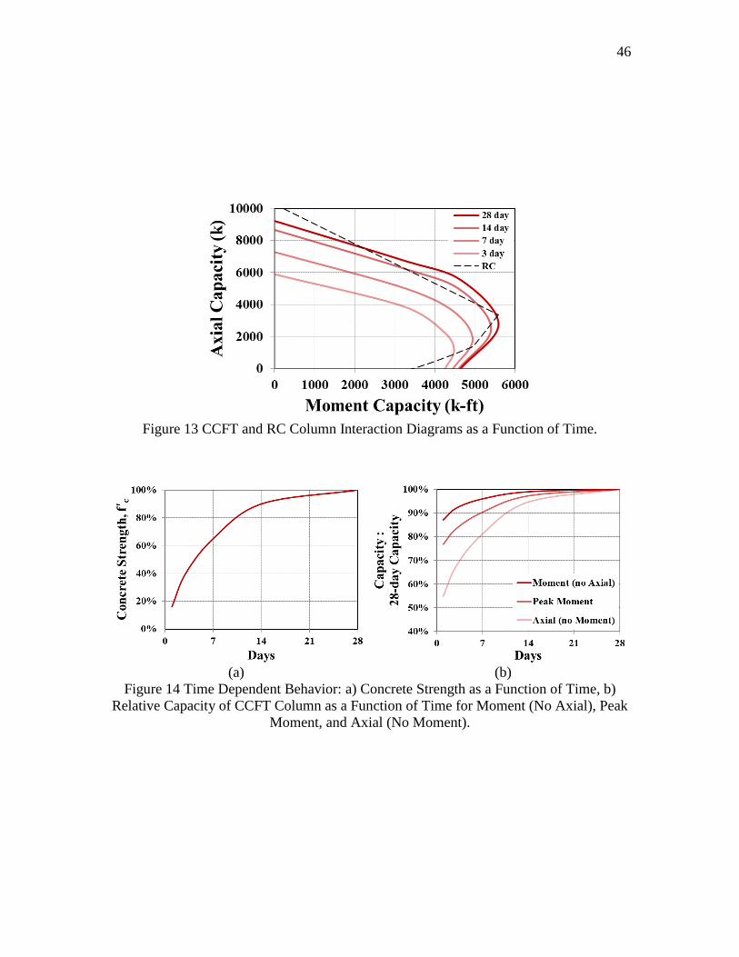
46

Figure 13 CCFT and RC Column Interaction Diagrams as a Function of Time.

(a) (b)

Figure 14 Time Dependent Behavior: a) Concrete Strength as a Function of Time, b)

Relative Capacity of CCFT Column as a Function of Time for Moment (No Axial), Peak

Moment, and Axial (No Moment).

47

Figure 15 CFST64 Experimental and Predicted Analytical Hysteretic Behavior (under

Static Cyclic Loading) and Monotonic Backbone Curve.

Modified from Marson, J.; Bruneau, M., Cyclic Testing of Concrete-Filled Circular Steel

Bridge Piers having Encased Fixed-Based Detail. Journal of Bridge Engineering 2004,

January/February.


Static Cyclic Loading) and Monotonic Backbone Curve.



January/February.

48


Static Cyclic Loading) and Monotonic Backbone Curve, θ = 0.15.



January/February.





January/February.

49





January/February.





January/February.

50

Figure 21 Hysteresis of Proposed CCFT at 3 and at 28 Days.


51


Figure 24 Hysteresis of Proposed CCFT at 28 Days.

52

Figure 25 Incremental Dynamic Analysis of Proposed CCFT at 3 Days.


53



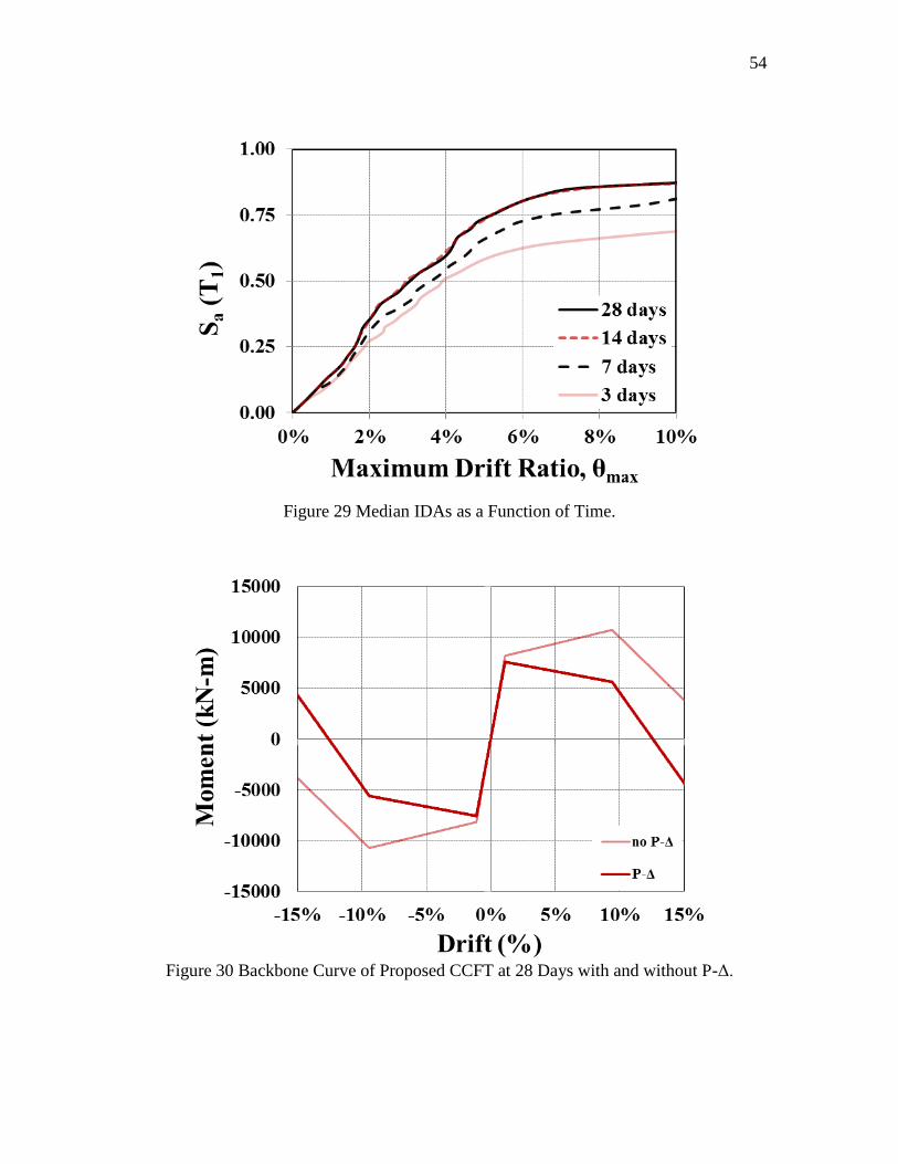
54

Figure 29 Median IDAs as a Function of Time.

Figure 30 Backbone Curve of Proposed CCFT at 28 Days with and without P-Δ.

55

Figure 31 Quasistatic Cyclic Loading (Peak-Oriented Hysteretic Curve) of Proposed

CCFT at 28 Days with and without P-Δ.

Figure 32 Dynamic Loading (Peak-Oriented Hysteretic Curve) of Proposed CCFT at 28

Days with and without P-Δ, Moment vs. Drift (Unscaled GM).

56


Days with and without P-Δ, Drift vs. Time (Unscaled GM).


Days with and without P-Δ, Moment vs. Drift (GM Scaled to 2).

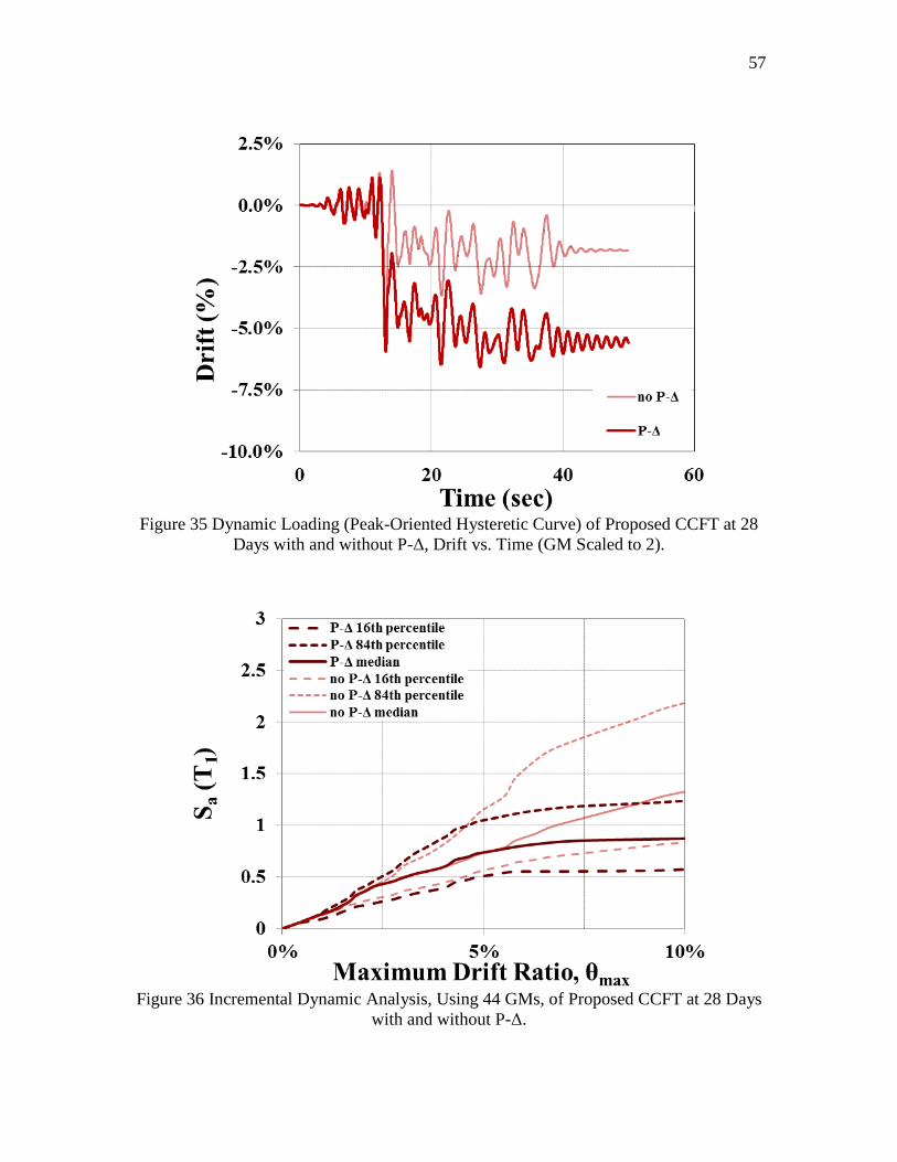
57


Days with and without P-Δ, Drift vs. Time (GM Scaled to 2).

Figure 36 Incremental Dynamic Analysis, Using 44 GMs, of Proposed CCFT at 28 Days

with and without P-Δ.

58

Table 2 Design-Basis Bridge RC Column Data

Reprinted with permission from Integrated Probabilistic Performance-Based Evaluation

of Benchmark Reinforced Concrete Bridges; by Kevin R. Mackie, John-Michael Wong,

and Bozidar Stojadinovc; PEER Report 2007/09; published January 2008 by the Pacific

Earthquake Engineering Research Center, University of California, Berkeley.

59

Table 3 Summary Data for Proposed CCFT as a Function of Time

Table 4 Cyclic Deterioration Parameters for CCFT

CCFT28 CCFT14 CCFT7 CCFT3

D/t

h (in)

As/Ac

% concrete strength 100% 90% 65% 40%

f'c (ksi) 5.2 4.68 3.38 2.08

ΔAISC (in) 10.1 10.3 10.8 11.6

ΔAASHTO (in) 12.7 12.8 13.3 14.0

θ (= PΔ/Vh) 0.072 0.073 0.076 0.080

Py (AISC Pn) (k) 9213 8659 7275 5890

P/Py 0.19 0.21 0.25 0.30

Mp (AISC) (k-ft) 5258 5180 4943 4345

Mp/My

My (k-ft) 6039 5949 5677 4990

My,P-Δ(My(1-θ))(k-ft) 5602 5513 5245 4592

Mc/My

Mc (k-ft) 7851 7734 7380 6487

Fy (= My/h) (k) 275 270 258 227

Fy/W 0.12 0.11 0.11 0.10

k (k/in) 94 93 89 85

T1(2π(m/k)1/2

)(sec) 1.4101 1.4188 1.4446 1.4799

T1(OpenSees)(sec) 1.4097 1.4185 1.4443 1.4795

0.87

1.3

0.07

64

264

Plastic rotational capacity, θp 0.08

Post-capping rotational capacity, θpc 0.1

Residual strength ratio, Mr 0.4

Ultimate rotational capacity, θu 0.4

Basic strength deterioration, Λs 4.0

Unloading stiffness deterioration, Λk 2.5

Accelerated reloading stiffness deterioration, Λa 1.6

Post-capping strength deterioration, Λd 0.57

EFFECT OF TEMPORARY CONDITIONS ON CIRCULAR

CONCRETE FILLED STEEL TUBE COLUMNS’ SEISMIC

PERFORMANCE

The time required for the column’s concrete to meet the design compressive

strength creates a temporal condition if the bridge is open to traffic before 28 days. The

ultimate goal of this study is to estimate the seismic probability of failure for this

temporary condition. The alternatives for developing seismic criteria for temporary

conditions include i) the use of standard seismic loads with a relaxed acceptance criteria,

or ii) reduction of seismic loads with a standard design criteria (Amin et al., 1999).

A reduced seismic load ( ) can be achieved by several approaches that are

controversial due to the illogical implications for temporary conditions that may arise

from arbitrarily discretizing a permanent condition, as well as the inability to provide

constant failure or fatality frequencies. In the case of CCFT columns, the temporal

conditions are clearly defined (i.e., the days the concrete needs to reach the design

compressive strength), and arbitrary discretizations of time can be excluded. Thus, s

are obtained following the approach presented by Amin et al. (Amin et al., 1999, Amin

and Jacques, 1994) in which:

( 15)

where is the design basis seismic load, and is a reduction factor that depends on

61

the duration of the temporary condition. In this study, it is conservatively assumed that

= 1/12 (representing about 1 month) for the three temporary conditions at 3, 7, and 14

days.

Regarding the system’s capacity, for the CCFT at 28 days (Figure 29), the median

collapse capacity is 0.88 g, and the standard deviation of the log of the collapse

capacity 0.420. This dispersion on collapse capacity due to RTR variability

is practically the same for CCFT columns with concrete cured for 7 and 14 days. For

CCFT at 3 days, the dispersion is slightly higher ( 0.422).

The mean annual frequency of collapse ( ) can be expressed as the mean

annual frequency of the strong motion intensity ( ) being larger than the collapse

capacity (i.e., ), multiplied by the probability of having such a strong motion intensity

(i.e., ( )),

∫ ( ) |

|

( 16 )

The above equation was solved by numerical integration for the four CCFT

columns to determine the probability of failure.

Figure 37 shows the mean hazard curve ( ) assuming the bridge is located in

Salt Lake City, Utah, as well as the reduced hazard curve for evaluation of temporary

conditions. Figure 38 presents the fragility curves of the CCFT columns, ( ) at the

collapse capacity limit state that was used to obtain the probability of failure. The

numerical integration of the hazard curve and the CCFT columns at 3, 7, and 14

days, resulted in the values for as a function of time listed in Table 5. Those values in

bold text are the values proposed for use in this study.

62

For the CCFT column at 28 days and the original hazard curve, the computed

probability of failure, , was 1.32 x 10-4

. The proposed values for for 1 month

(using = 1/12 for 14, 7, and 3 days) are significantly lower than that of the design

CCFT column ( 1.32 x 10-4

), indicating that the capacity reduction of CCFT columns

at 3, 7, and 14 days is compensated by assuming a temporary condition.

Note that the hazard curve reduction factor could have been assumed as = 1/2

(i.e., a temporary condition of 6 months), and the critical CCFT at 3 days would render a

1.1 x 10-4

, still lower than the probability of failure for the base case. This

conservative calculation implies that the temporary condition could last for 6 months,

instead of 3 days, and the probability of failure would not exceed that of the base case.

63

Figure 37 Hazard Curve for Salt Lake City, Utah for T1=1.40 s. for DBSL and RSL

Conditions.

Figure 38 Fragility Curves for the Four CCFT Evaluated Condition.

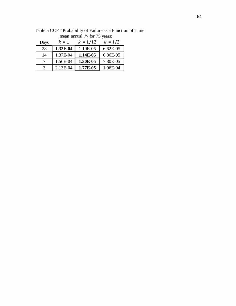
64

Table 5 CCFT Probability of Failure as a Function of Time

Days k = 1 k = 1/12 k = 1/2

28 1.32E-04 1.10E-05 6.62E-05

14 1.37E-04 1.14E-05 6.86E-05

7 1.56E-04 1.30E-05 7.80E-05

3 2.13E-04 1.77E-05 1.06E-04

mean annual for 75 years:

65

CONCLUSIONS

The study assesses the effect of partial concrete compressive strength on the

seismic performance of CCFT bridge columns prior to full concrete compressive strength

being achieved. If the bridge needs to be open to traffic after a few days, the time

required for the columns’ concrete to meet the design compressive strength creates a

temporary condition. The research evaluates whether this temporary condition increases

the seismic probability of failure using as the criterion a comparison of CCFT columns

under permanent conditions subjected to DBSL with that of temporary conditions

subjected to RSL.

The first phase of the study addresses the design of CCFT columns. These

components may require a third less cross-sectional area than the original RC columns to

achieve similar capacity under combined axial and bending forces. Because of the highly

localized failure mode of CCFT columns, concentrated plasticity models can reliably

predict the nonlinear performance of these components up to the collapse limit state. This

study calibrates for first time the deteriorating nonlinear parameters required for these

numerical simulations.

It is observed that the gain in concrete strength is not as critical for CCFT

columns as in RC columns. Concrete only reaches about 40% of its design strength after

3 days, where the CCFT column achieves 92% and 68% of its full pure moment capacity

and full pure axial capacity, respectively, on day 3. Thus, the steel tube is largely

66

responsible for initial capacity of the CCFT, as long as the concrete provides lateral

constraint preventing buckling failure.

Based on the incremental dynamic analysis (IDA) analysis, the collapse capacity

of CCFT columns at 3, 7, and 14 days correspond to 80, 93, and 98% of the CCFT

collapse capacity at 28 days, when the concrete is expected to reach its design

compressive strength. If a conservative temporary condition of 1 month is assumed for

CCFT columns with less than 1 month of curing, the probability of failure for CCFT

columns at 3, 7, and 14 days is about one order of magnitude smaller than that for the

CCFT column over the lifespan of 75 years.

RECOMMENDATIONS FOR FUTURE RESEARCH

Experimental Testing

There are two areas of underrepresented experimental research on CCFT which

are applicable to this project. For research applicable to highway bridges, the current

experimental data are missing sufficient number of normal strength concrete / normal

strength steel experiments performed with appropriate diameter / steel tube thickness

( ) ratio and height / diameter ratio. In addition, experimental testing needs to include

specimens tested under monotonic loading for the creation of backbone curves.

Bond Strength as a Function of Concrete Age

Were experiments to be conducted, it would be of particular applicability to the

current research to subject multiple identical specimens to the same loading protocol at

various points in the concrete curing time – likely at 3, 7, 14, as well as 28 days. The

objective would be to determine the seismic performance of the CCFTs as a function of

time, but additionally, to determine the relation of concrete curing time to the bond

strength between the concrete core and the steel tube.

Parameter Study for Hysteretic Modeling of CCFT

Nonlinear deteriorating hysteretic parameters were found for modeling of CCFTs

of interest. However, these parameters will change depending on the stability coefficient,

68

; the diameter to thickness ratio, ; and the ratio of area of steel to area of concrete,

. Determination of specifically what factors have the greatest influence and what

the corresponding ranges of the plastic spring parameters would be potential future

research.

APPENDIX A

COMPARATIVE CCFT DATA

70

Table 6 Proposed CCFT Column as a Function of Time and Experimental CCFT Data

CCFT28 CCFT14 CCFT7 CCFT3 CFST64 CFST51 CFST34 CFST42

D/t 73.89 58.88 43.18 42.78

D (in) 16 12.75 12.75 16

t (nominal) (in) 0.25 0.25 0.375 0.375

t (measured) (in) 0.22 0.22 0.30 0.37

h (in)

As (in2) 10.74 8.53 11.55 18.36

Ac (in2) 190.32 119.15 116.12 182.70

As/Ac 5.64% 7.16% 9.95% 10.05%

Is (in4) 334.41 167.47 224.15 560.71

Ic (in4) 2882.58 1129.74 1073.06 2656.28

P (k) 225 360 409 409

self-weight (k) 5 3 3 5

W (k) 299 472 536 539

Fy (specified) (ksi) 50.76 50.76 50.76 50.76

Fy (tested) (ksi) 64.11 58.02 60.19 73.24

Fu (ksi) 81.51 78.76 74.69 86.30

εs (tested steel strain) 0.0030 0.0034 0.0024 0.0043

Es (ksi)

% concrete strength - 90% 65% 40% - - - -

f'c (ksi) 5.2 4.68 3.38 2.08 5.35 5.09 5.88 5.09

Ec (ksi) 4552 4376 3873 3229 4603 4514 4766 4517

C3 (AISC factor) 0.71 0.73 0.78 0.78

EIeff,AISC (k-in2) 7.22E+08 7.09E+08 6.73E+08 6.26E+08 1.91E+07 8.60E+06 1.05E+07 2.57E+07

EIeff,AASHTO (k-in2) 5.749E+08 5.678E+08 5.477E+08 5.219E+08 1.501E+07 6.897E+06 8.546E+06 2.106E+07

0.8EIeff,AASHTO(k-in2) - - - - 1.20E+07 5.52E+06 6.84E+06 1.68E+07

Sa

V (= WSa) (k) 149.99 236.88 269.26 270.55

ΔAISC (in) 10.10 10.29 10.84 11.65 1.70 5.97 5.56 2.28

ΔAASHTO (in) 12.69 12.85 13.32 13.98 2.71 9.30 8.53 3.48

θ (= PΔ/Vh) 0.072 0.073 0.076 0.080 0.047 0.163 0.150 0.061

Py (AISC Pn) (k) 9213 8659 7275 5890 1657 1070 1344 2229

P/Py 0.19 0.21 0.25 0.30 0.14 0.34 0.30 0.18

Mp (AISC) (k-ft) 5258 5180 4943 4345 386 220 292 674

Mp/My 0.86 0.81 0.88 0.93

My (k-ft) 6039.22 5949.38 5676.91 4989.88 449.91 271.42 331.90 722.07

My,P-Δ(My(1-θ))(k-ft) 5602 5513 5245 4592 429 227 282 678

Mc/My

Mc (k-ft) 7851 7734 7380 6487 585 353 431 939

Fy (= My/h) (k) 275 270 258 227 62.34 37.61 45.99 100.04

Fy/W 0.12 0.11 0.11 0.10 0.21 0.08 0.09 0.19

m (k-s2/in) 0.60 0.94 1.07 1.07

k (k/in) 93.73 92.58 89.30 85.10 55.43 25.48 31.57 77.80

T1(2π(m/k)1/2

)(sec) 1.4101 1.4188 1.4446 1.4799 0.6511 1.2070 1.1560 0.7382

T1(OpenSees)(sec) 1.4097 1.4185 1.4443 1.4795 0.6514 1.2069 1.1559 0.7379

bold terms implemented into concentrated plasticity model

-

1121

50

-

64

39

0.61

-

264

4.72

86.61

13543

100017

0.72

6.56%

1.3

0.87

2369

0.502

1189

29000

1792

30

65

73

APPENDIX B

BUCKLING ANALYSIS CALCULATIONS

APPENDIX C

INTERACTION DIAGRAM CALCULATIONS

76

Table 7 P-M Capacities of CCFT

Reprinted with permission from Gerschwindner, L. F., Discussion- Limit State Response

of Composite Columns and Beam-Columns Part II- Application of Design Provisions for

the 2005 AISC Specification. Engineering Journal 2010, Second Quarter, 131.

77

Table 8 Calculated P-M Parameters of Proposed CCFT Column

CCFT28 CCFT14 CCFT7 CCFT3

d (D) (in) 39 39 39 39

t (in) 0.61 0.61 0.61 0.61

h (in) 37.78 37.78 37.78 37.78

hn (in) 8.6 8.2 6.9 5.2

hE (in) 13.7 13.5 12.9 12.0

Fy (ksi) 50 50 50 50

Fu (ksi) 65 65 65 65

Es (ksi) 29000 29000 29000 29000

As (in2) 73 73 73 73

Is (in4) 13543 13543 13543 13543

Zs (in3) 898 898 898 898

ZsB (in3) 801 810 836 864

ZsE (in3) 617 627 656 693

Ss (in3) 695 695 695 695

Ks (k/in) 585 585 585 585

Knominal 1 1 1 1

rs (in) 13.6 13.6 13.6 13.6

L (h) (in) 264 264 264 264

Fe 757 757 757 757

Fcr 48.6 48.6 48.6 48.6

θ (rad) 2.20 2.25 2.39 2.59

θ2 (rad) 1.51 1.55 1.64 1.76

dc (in) 37.78 37.78 37.78 37.78

Ac (in2) 1121 1121 1121 1121

Ic (in4) 100017 100017 100017 100017

f'c (ksi) 5.20 4.68 3.38 2.08

wc (lbs/cf) 145 145 145 145

*Ec (ksi) 4552 4376 3873 3229

Zc (in3) 8988 8988 8988 8988

ZcB (in3) 6363 6597 7252 8004

ZcE (in3) 2913 3060 3509 4126

Kc (k/in) 7423 6680 4825 2969

Q (in3) 449 449 449 449

Z (in3) 898 898 898 898

78

Table 9 Calculated P-M Capacities of Proposed CCFT and Design Basis RC Columns

Leon/Hajjar (AISC) ACI

Pn (k) Mn (k-ft) Pn (k) Mn (k-ft) Pn (k) Mn (k-ft) Pn (k) Mn (k-ft) Pn (k) Mn (k-ft) AISC (ACI)

A 9213 0 8659 0 7275 0 5890 0 10259 0 A (A)

E 6790 3170 6287 3180 5054 3205 3877 3227 3357 5591 E (B)

C 5538 4645 4984 4598 3600 4454 2215 4260

D 2769 5593 2492 5408 1800 4945 1108 4483 3346 5585 D (C )

B 0 4645 0 4598 0 4454 0 4260 1442 4977 (CD)

linear interpolation to determine where on curve the applied axial load falls: 1281 4866 (D)

1792 5258.4 1792 5180.2 1792 4943 1792 4344.8 -88 3347 (E)

-2418 0 (F)

RCCCFT28 CCFT14 CCFT7 CCFT3

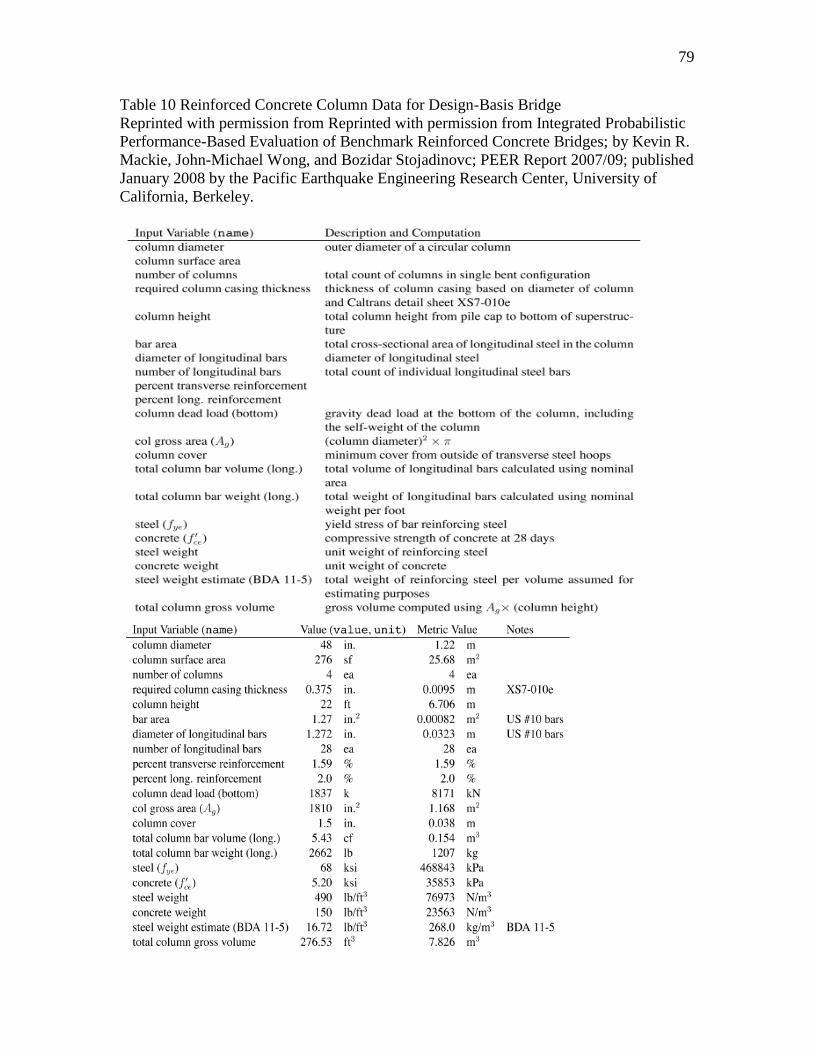
79

Table 10 Reinforced Concrete Column Data for Design-Basis Bridge

Reprinted with permission from Reprinted with permission from Integrated Probabilistic

Performance-Based Evaluation of Benchmark Reinforced Concrete Bridges; by Kevin R.

Mackie, John-Michael Wong, and Bozidar Stojadinovc; PEER Report 2007/09; published

January 2008 by the Pacific Earthquake Engineering Research Center, University of


REFERENCES

AASHTO, AASHTO LRFD Bridge Design Specifications. American Association of

State Highway and Transportation Officials: Washington, D.C., 2012.

ACI, Building Code Requirements for Structural Concrete (ACI 318-08) and

Commentary. American Concrete Institute: 2008.

Adam, C.; Ibarra, L. F.; Krawinkler, H., Evaluation of P-Delta Effects in Non-

Deteriorating MDOF Structures from Equivalent SDOF Systems. In Proceedings of the

13th World Conference on Earthquake Engineering, 2004; Vol. 1.

AISC, Seismic Provisions for Structural Steel Buildings. American Institute of Steel

Construction: 2010a.

AISC, Steel Construction Manual. American Institute of Steel Construction: 2010b.

Amin, M.; Budnitz, R. J.; Cornell, C. A.; Kennedy, R. P.; Olson, D. E.; Tang, H. T.,

Reduced Seismic Loads for Temporary Conditions. Nuclear Engineering and Design

1999, 192, 167-178.

Amin, M.; Jacques, L. V., Seismic Loading for Evaluation of Temporary Conditions in

Nuclear Power Plants. In Fifth U.S. National Conference on Earthquake Engineering,

Chicago, Illinois, 1994.

An, Y.-F.; Han, L.-H.; Zhao, X.-L., Behaviour and Design Calculations on Very Slender

Thin-Walled CFST Columns. Thin-Walled Structures 2012, 53, 161-175.

ATC, Recommended Seismic Design Criteria for New Steel Moment-Frame Buildings.

Committee, S. J. V. G. D., Ed. Federal Emergency Management Agency: Washington,

DC, 2000a.

ATC, Recommended Seismic Evaluation and Upgrade Criteria for Welded Steel Moment

Frame Buildings. Committee, S. J. V. G. D., Ed. Federal Emergency Management

Agency: Washington, DC, 2000b.

ATC, Quantification of Building Seismic Performance Factors. Applied Technology

Council: Washington D.C., 2009.

90

Bernal, D., Amplification Factors for Inelastic Dynamic P–Δ Effects in Earthquake

Analysis. Earthquake Engineering & Structural Dynamics 1987, 15 (5), 635-651.

Boggs, D. W.; Peterka, J. A., Wind Speeds for Design of Temporary Structures. In 10th

ASCE Structures Congress, Structures Congress '92 Compact Papers: San Antonio,

Texas, 1992.

Boyd, P. F.; Cofer, W. F.; Mclean, D. I., Seismic Performance of Steel-Encased Concrete

Columns under Flexural Loading. ACI Structural Journal 1995, 92 (3).

Clough, R.; Johnston, S., Effect of Stiffness Degradation on Earthquake Ductility

Requirements. In Japan Earthquake Engineering Symposium, Tokyo, Japan, 1966.

Cornell, C. A.; Bandyopadhyay, K. K., Should We Relax Seismic Criteria for Shorter

System Exposure Times? In ASME Pressure Vessels and Piping Conference, Montreal,

1996.

Elremaily, A.; Azizinamini, A., Behavior and Strength of Circular Concrete-Filled Tube

Columns. Journal of Constructional Steel Research 2002, 58, 1567-1591.

Gerschwindner, L. F., Discussion- Limit State Response of Composite Columns and

Beam-Columns Part II- Application of Design Provisions for the 2005 AISC

Specification. Engineering Journal 2010, Second Quarter, 131.

Goode, C. D., ASCCS Database of Concrete Filled Steel Tube Column Tests. 2013.

Han, L.-H.; Wang, W.-D.; Tao, Z., Performance of Circular CFST Column to Steel Beam

Frames under Lateral Cyclic Loading. Journal of Constructional Steel Research 2011, 67

(5), 876-890.

Hassoun, M. N.; Al-Manaseer, A., Structural Concrete: Theory and Design. 2012.

Hill, H. J., Rational and Irrational Design Loads for Temporary Structures. Practice

Periodical on Structural Design and Construction 2004.

Ibarra, L. F.; Krawinkler, H., Global Collapse of Frame Structures under Seismic

Excitations. Pacific Earthquake Engineering Research Center: 2005.

Ibarra, L. F.; Medina, R. A.; Krawinkler, H., Hysteretic Models that Incorporate Strength

and Stiffness Deterioration. Earthquake Engineering & Structural Dynamics 2005, 34

(12), 1489-1511.

Jennings, P. C.; Husid, R., Collapse of Yielding Structures During Earthquakes. Journal

of Engineering Mechanics 1968.

Ketchum, M.; Chang, V.; Shantz, T. S., Influence of Design Ground Motion Level on

Highway Bridge Costs. 2004, (Project Number 6D01).

91

Kitada, T., Stability and Ductility of Steel Structures under Cyclic Loading. 1991, 3.

Kitada, T., Ductility and Ultimate Strength of Concrete-Filled Steel Members. 1992.

Kitada, T., Ultimate Strength and Ductility of State-of-the-Art Concrete-Filled Steel

Bridge Piers in Japan. Engineering Structures 1998, 20 (4), 347-354.

Knowles, R. B.; Park, R., Strength of Concrete Filled Steel Columns. Journal of the

Structural Division 1969.

Kosmatka, S. H.; Panarese, W. C., Design and Control of Concrete Mixtures. Portland

Cement Association: 2002.

Leon, R. T.; Hajjar, J. F., Limit State Response of Composite Columns and Beam-

Columns Part I- Formulation of Design Provisions for the 2005 AISC Specification.

Engineering Journal 2007, Fourth Quarter, 341.

Leon, R. T.; Hajjar, J. F., Limit State Response of Composite Beam-Columns -- Part II

Application. Engineering Journal 2008, 45 (1).

Leon, R. T.; Perea, T.; Hajjar, J. F.; Denavit, M. D., Concrete-Filled Tubes Columns and

Beam-Columns: A Database for the AISC 2005 and 2010 Specifications. 2011.

Liel, A. B.; Haselton, C. B.; Deierlein, G. G.; Baker, J. W., Incorporating Modeling

Uncertainties in the Assessment of Seismic Collapse Risk of Buildings. Structural Safety

2009, 31 (2), 197-211.

Lignos, D. G. Modified Ibarra-Medina-Krawinkler Deterioration Model with Peak-

Oriented Hysteretic Response (ModIMK Peak Oriented Material).

http://opensees.berkeley.edu/wiki/index.php/Modified_Ibarra-Medina-Krawinkler_

Deterioration_Model_with_Peak-

Oriented_Hysteretic_Response_(ModIMKPeakOriented_Material).

Lignos, D. G.; Krawinkler, H., Deterioration Modeling of Steel Components in Support

of Collapse Prediction of Steel Moment Frames under Earthquake Loading. Journal of

Structural Engineering 2011, 137 (11), 1291-1302.

Lignos, D. G.; Krawinkler, H., Sidesway Collapse of Deteriorating Structural Systems

Under Seismic Excitations. In The John A. Blume Earthquake Engineering Center,

Stanford University: 2012.

MacRae, G. A., P-Δ Effects on Single-Degree-of-Freedom Structures in Earthquakes.

Earthquake Spectra 1994, 10 (3), 539-568.

Marson, J. Cyclic Testing of Concrete-Filled Circular Steel Tube Bridge Columns having

Encased Fixed Based Detail. University of Ottawa, Ottawa, Canada, 2000.

http://opensees.berkeley.edu/wiki/index.php/Modified_Ibarra-Medina-Krawinkler_

92

Marson, J.; Bruneau, M., Cyclic Testing of Concrete-Filled Circular Steel Bridge Piers

having Encased Fixed-Based Detail. Journal of Bridge Engineering 2004,

January/February.

McKenna, F.; Fenves, G.; Scott, M. Open System for Earthquake Engineering

Simulation, University of California: Berkeley, CA, 2000.

Mindess, S.; Young, J. F.; Darwin, D., Concrete. 2003.

Olson, D. E.; Amin, M.; Jaques, L. V., Evaluation of Temporary Loads: Approach to

Justify Larger Loads with Less Effort. In Pressure Vessels and Piping Division (ASME),

1994; Vol. 285.

Ranzi, G.; Leoni, G.; Zandonini, R., State of the Art on the Time-Dependent Behaviour

of Composite Steel–Concrete Structures. Journal of Constructional Steel Research 2013,

80, 252-263.

Sivaselvan, M. V.; Reinhorn, A. M., Hysteretic Models for Deteriorating Inelastic

Structures. Journal of Engineering Mechanics 2000, 126 (6), 633-640.

Song, J.-K.; Pincheira, J. A., Spectral Displacement Demands of Stiffness and Strength-

Degrading Systems. Earthquake Spectra 2000, 16 (4), 817-851.

Sun, C.-K.; Berg, G. V.; Hanson, R. D., Gravity Effect on Single-Degree Inelastic

System. Journal of the Engineering Mechanics Division 1973, 99 (1), 183-200.

Vamvatsikos, D. IDA Matlab Running Routines for OpenSEES, 2011.

Vamvatsikos, D.; Cornell, C. A., Incremental Dynamic Analysis. Earthquake

Engineering & Structural Dynamics 2002, 31 (3), 491-514.

Vamvatsikos, D.; Cornell, C. A., Applied Incremental Dynamic Analysis. Earthquake

Spectra 2004, 20 (2), 523-553.

Vian, D.; Bruneau, M., Experimental Investigation of P-Delta Effects to Collapse During

Earthquakes. 2001.

Villaverde, R., Methods to Assess the Seismic Collapse Capacity of Building Structures:

State of the Art. Journal of Structural Engineering 2007, 133 (1), 57-66.

Winters-Downey, E.; Zuo, J.; Wang, M., Hollow Product, Solid Benefit. Modern Steel

Construction 2013.

Zhang, J.; Denavit, M. D.; Hajjar, J.; Lu, X., Bond Behavior of Concrete-Filled Steel

Tube (CFT) Structures. Engineering Journal 2012, 49 (4), 169-185.

Zhao, X.-L.; Han, L.-H.; Lu, H., Concrete-filled Tubular Members and Connections.

2010.

SEISMIC PERFORMANCE OF CIRCULAR CONCRETE …

Documents

Transcript of SEISMIC PERFORMANCE OF CIRCULAR CONCRETE …