CMPWG-II, UF 1

PENELOPE (v. 2006)A coupled electron-photon transport code

Francesc Salvat, José M Fernández-Varea, Josep Sempau,

Xavier Llovet, David Bote

CMPWG-II, UF 2

Outline

PENELOPE Photon interactions and transportElectron interactionsElectron transportConstructive quadric geometrySome applications

CMPWG-II, UF 3

PENELOPE

PENetration and Energy LOss ofPositrons and Electrons... and photons

F Salvat, JM Fernández-Varea, J Sempau

A general-purpose Monte Carlo code

Distributed by the OECD-NEA Data Bank, Paris (∼600 registered users)

http://www.nea.fr/lists/penelope.html

Available also from RSICC, and from the authors

CMPWG-II, UF 4

Main features

All kinds of interactions (except nuclear reactions) in the energy range

from ∼ 50 eV to 109 eV(covered by the database)

Implements the most accurate physical models available (limited only by the required generality)

Simulates electrons and positrons (tunable mixed scheme) and photons (detailed, interaction by interaction)

Simulates fluorescent radiation from K, L and M shells

Includes a flexible geometry package (constructive quadric geometry)

Electron and positron transport in external magnetic and electric fields (in matter)

CMPWG-II, UF 5

Specific features

PENELOPE evolved from low-energy (keV) electron-transport MC codes, which were used in the late 1980s to simulate electron microscopy and conversion-electron Mössbauer spectroscopy.

The main difference is in the electron transport mechanics

Our main research is in theoretical atomic physics. We develop models and codes for calculating interaction cross sections. When a model is proven to be robust and general, we generate an extensive database and plug it into PENELOPE, replacing older models.

PENELOPE is evolving continuously. Specificities of different materials

PENELOPE is structured as a subroutine package (in the style of most codes used in atomic and nuclear physics).

The user has complete access to the physical parameters... Example main programs are provided (PENSLAB, PENCYL, PENMAIN)

All Monte Carlo codes, including PENELOPE, are plagued with approximations, both in the physical interaction models and in the electron transport algorithms

CMPWG-II, UF 6

Random sampling (RITA method)Piecewise Rational Inverse Transform with Aliasing. Adaptive, very accurate

32 points:

CMPWG-II, UF 7

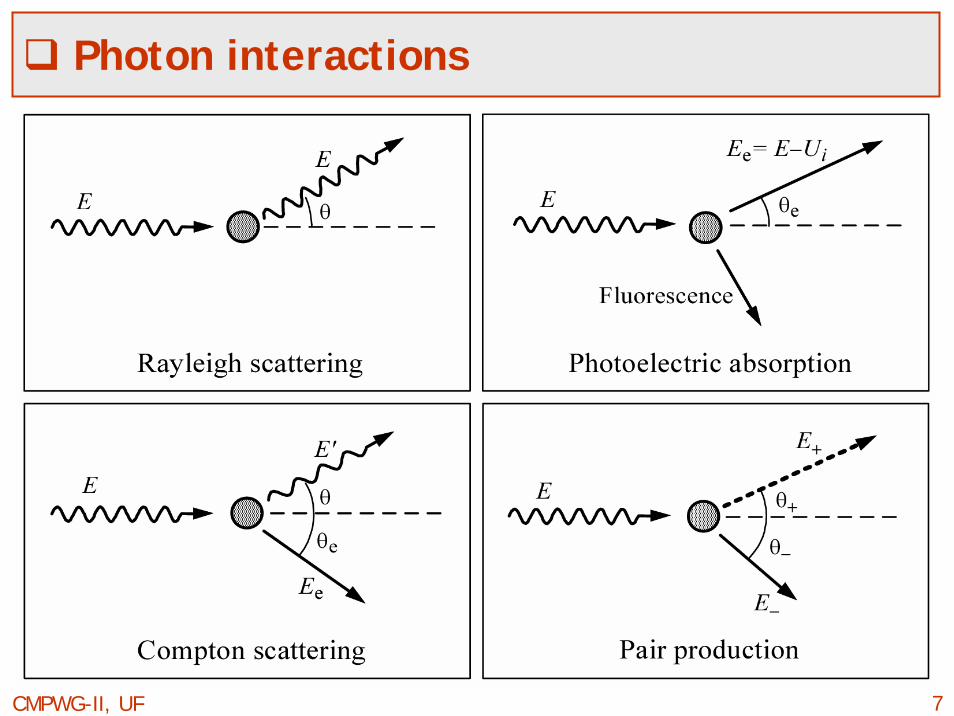
Photon interactions

CMPWG-II, UF 8

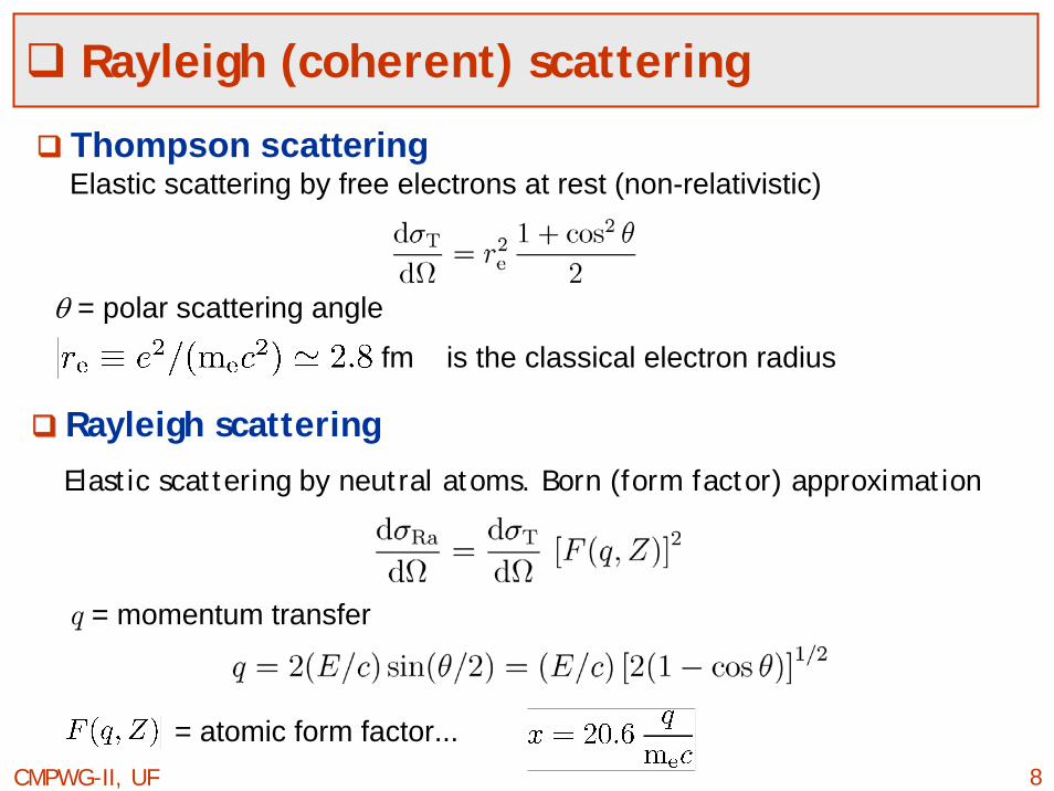
Rayleigh (coherent) scattering

Thompson scatteringElastic scattering by free electrons at rest (non-relativistic)

θ = polar scattering angle

fm is the classical electron radius

Rayleigh scatteringElastic scattering by neutral atoms. Born (form factor) approximation

q = momentum transfer

= atomic form factor...

CMPWG-II, UF 9

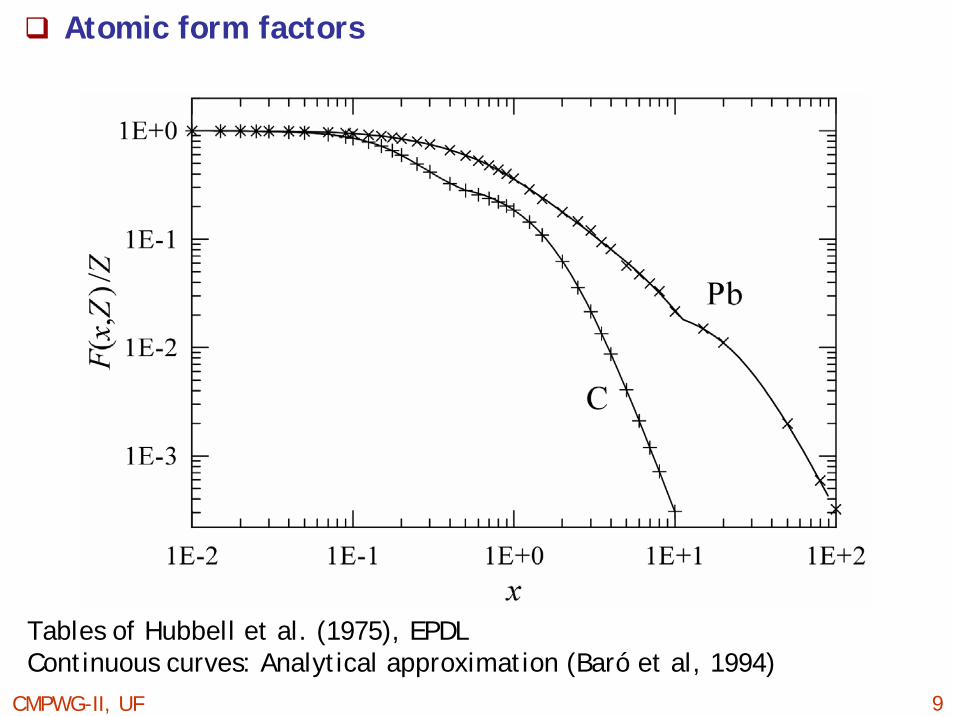
Tables of Hubbell et al. (1975), EPDLContinuous curves: Analytical approximation (Baró et al, 1994)

Atomic form factors

CMPWG-II, UF 10

Photoelectric effect

LLNL’s EPDL ’97 database (Cullen et al., 1997)

Scofield’s calculation of

- independent-electron model: Dirac-Hartree-Fock-Slater- 1st-order perturbation theory- matrix elements

Hubbell’s compilation of

i = K, L1-L3, M1-M5 shells

Large uncertainties below ∼ 1 keV

Initial direction of photoelectrons.Sauter relativistic DCS for ionization of hydrogenic ions

(approximately valid for K-shell electrons).

CMPWG-II, UF 11

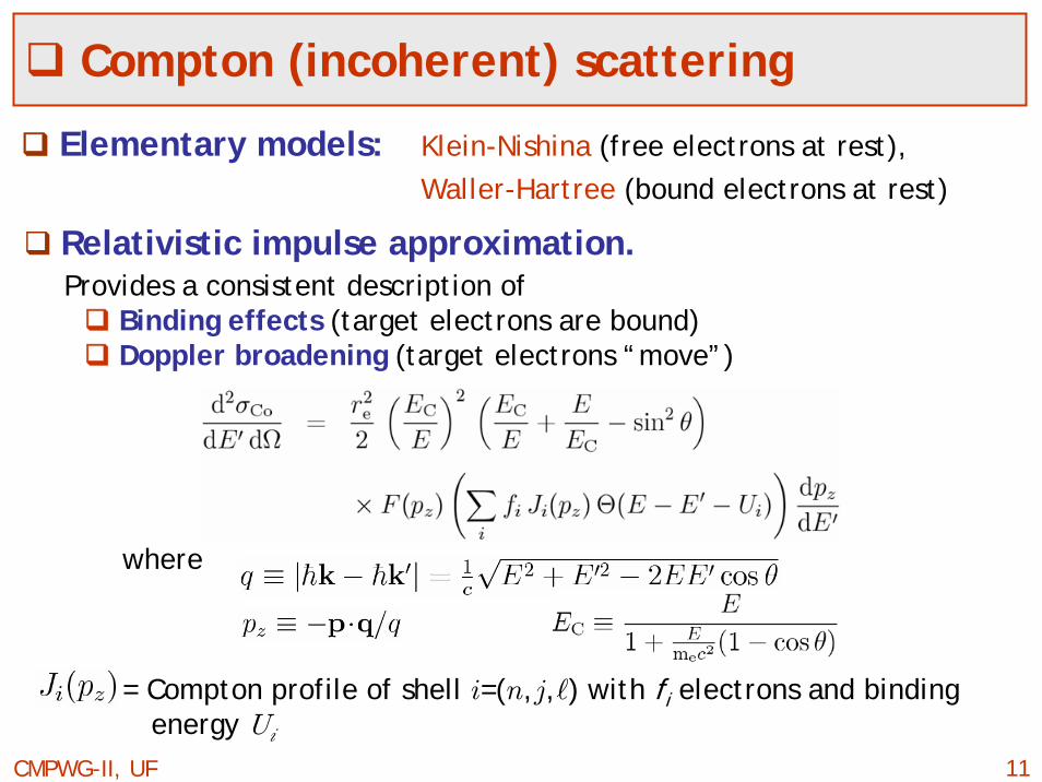
Compton (incoherent) scattering

Relativistic impulse approximation.Provides a consistent description of

Binding effects (target electrons are bound)Doppler broadening (target electrons “move”)

where

= Compton profile of shell i=(n,j,`) with fi electrons and bindingenergy Ui

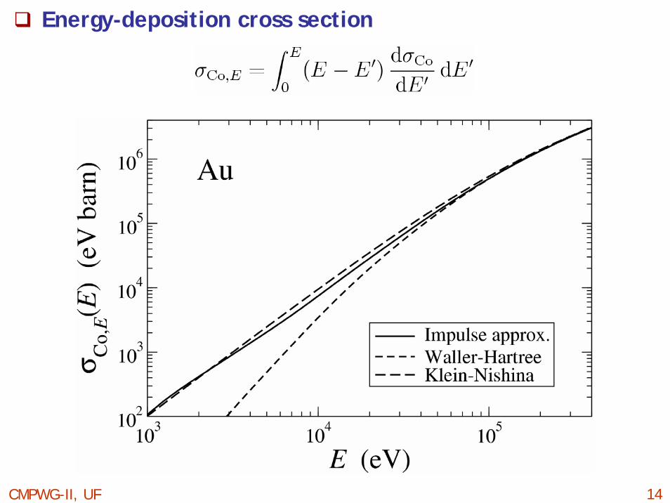
Elementary models: Klein-Nishina (free electrons at rest), Waller-Hartree (bound electrons at rest)

CMPWG-II, UF 12

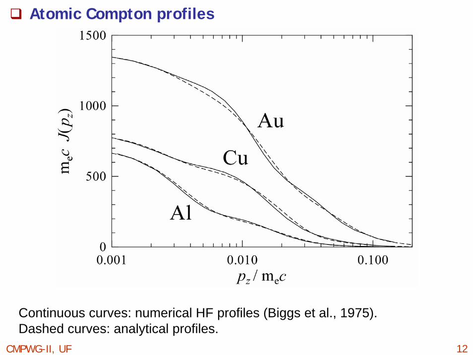
Continuous curves: numerical HF profiles (Biggs et al., 1975).Dashed curves: analytical profiles.

Atomic Compton profiles

CMPWG-II, UF 13

Continuous curves: calculated with numerical HF profiles.Dashed curves: calculated with the analytical profiles.

EC

EC

Double DCS for 10 keV photons in Al

CMPWG-II, UF 14

Energy-deposition cross section

CMPWG-II, UF 15

Electron-positron pair production

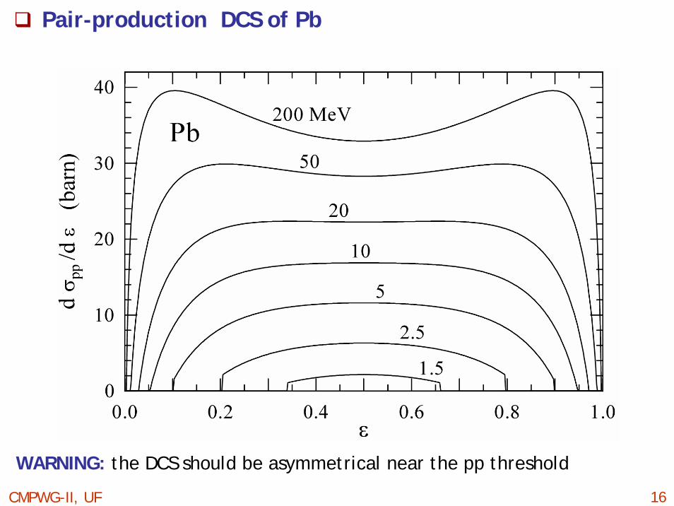
Bethe-Heitler DCS Born approximation with exponential screeningHigh-energy Coulomb correctionEmpirical (fitted) low-energy correctionAttenuation coefficient from EPDL (pair + triplet)

CMPWG-II, UF 16

WARNING: the DCS should be asymmetrical near the pp threshold

Pair-production DCS of Pb

CMPWG-II, UF 17

Partial and total mass-attenuation coefficients

CMPWG-II, UF 18

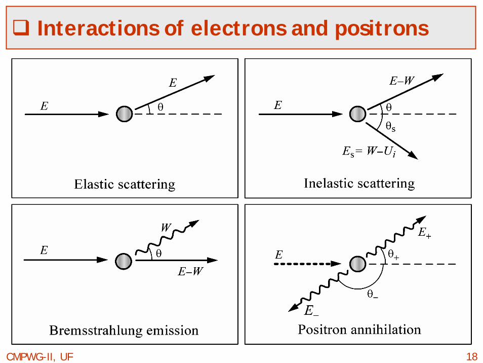
Interactions of electrons and positrons

CMPWG-II, UF 19

Elastic collisions

Polar angular deflection: θ, scattering angle or

Collisions without electronic excitation of the target.Because of the smallness of the electron mass (<< Mnuc ≈ 3600 Z me)recoil energy losses are negligible.

2cos1 θμ −

≡

Static-field approximation: Potential scattering theoryV(r) = electrostatic interaction (+ local exchange for e−)

Relativistic (Dirac) partial-wave analysis:

CMPWG-II, UF 20

Numerical Database: ICRU 77, NIST, CPC (ELSEPA)

CMPWG-II, UF 21

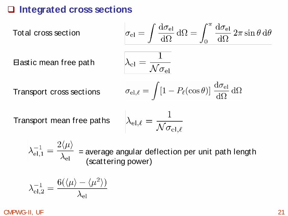
Total cross section

Elastic mean free path

Transport cross sections

Transport mean free paths

= average angular deflection per unit path length(scattering power)

Integrated cross sections

CMPWG-II, UF 22

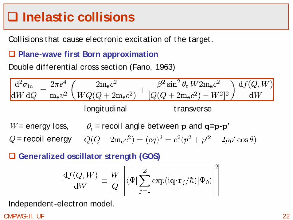
Inelastic collisions

Plane-wave first Born approximationDouble differential cross section (Fano, 1963)

W = energy loss, θr = recoil angle between p and q=p-p’

Generalized oscillator strength (GOS)

Q = recoil energy

Independent-electron model.

longitudinal transverse

Collisions that cause electronic excitation of the target.

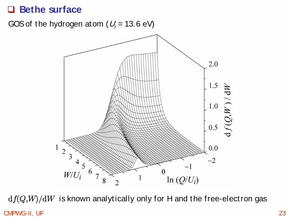
CMPWG-II, UF 23

Bethe surfaceGOS of the hydrogen atom (Ui = 13.6 eV)

df(Q,W)/dW is known analytically only for H and the free-electron gas

CMPWG-II, UF 24

Sternheimer-Liljequist GOS modelSum of “delta” oscillators (one per each electron shell)

Satisfies: 1) Bethe sum rule:

2) Mean-ionization energy

“delta” oscillator:

CMPWG-II, UF 25

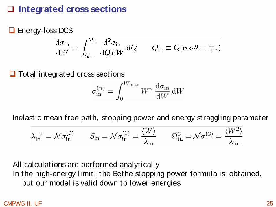
Energy-loss DCS

Total integrated cross sections

Inelastic mean free path, stopping power and energy straggling parameter

All calculations are performed analyticallyIn the high-energy limit, the Bethe stopping power formula is obtained,

but our model is valid down to lower energies

Integrated cross sections

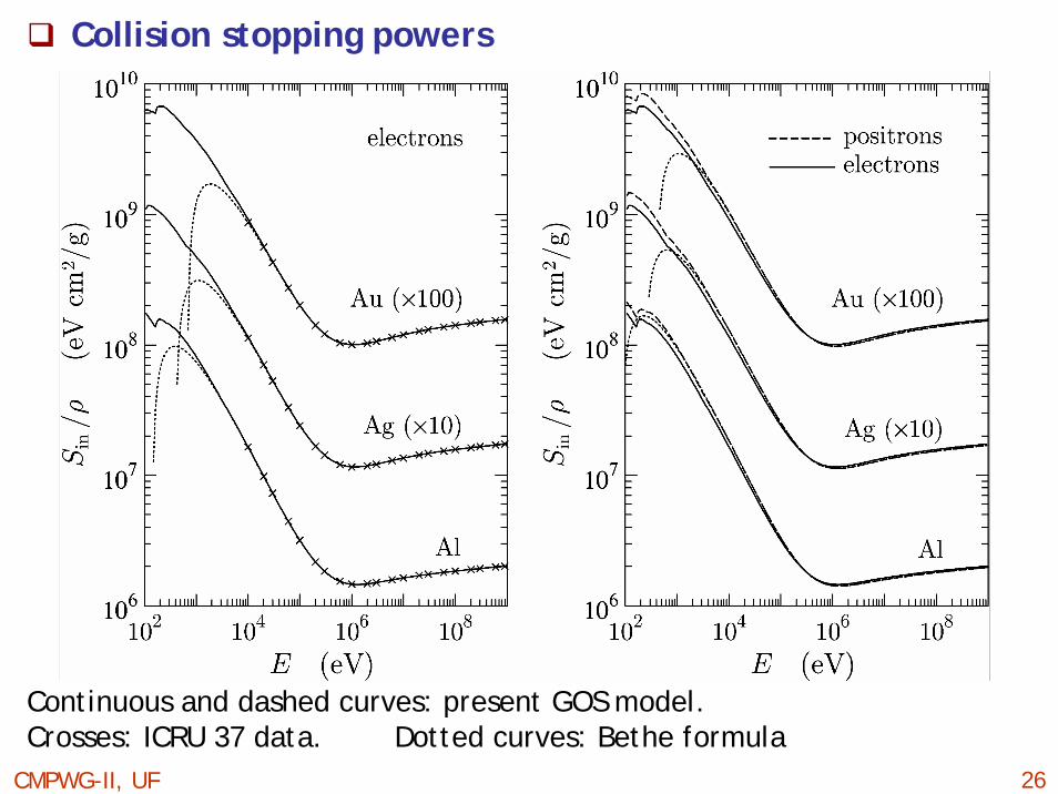
CMPWG-II, UF 26

Continuous and dashed curves: present GOS model.Crosses: ICRU 37 data. Dotted curves: Bethe formula

Collision stopping powers

CMPWG-II, UF 27

Bremsstrahlung emission

Bethe-Heitler energy-loss DCS (Plane-wave Born approximation)

Charged projectiles, accelerated by the electrostatic field of the target atom emit electromagnetic radiation

DCS for electrons:

“scaled” bremsstrahlung DCS

κ=W/E reduced photon energy ∈(0,1)

Seltzer and Berger (1986) tables of χ(Z,E,κ) - electron-nucleus: Bethe-Heitler DCS

combined with partial-wave calculations by Pratt et al. (1977)- electron-electron: Haug (1975) theory

CMPWG-II, UF 28

Scaled bremsstrahlung DCSs for e-

Seltzer and Berger (1986)

CMPWG-II, UF 29

Mean free path (restricted)

Radiative stopping power

Bremsstrahlung straggling parameter

Integrated cross sections

CMPWG-II, UF 30

Continuous and dashed curves: present model.Crosses: ICRU 37 data.

Radiative stopping powers

CMPWG-II, UF 31

Double DCS

shape function (pdf, normalized to unity)

Partial-wave calculations of shape functions (Kissel et al., 1983):Z = 2, 8, 13, 47, 79, 92E = 1, 5, 10, 50, 100, 500 keVκ = 0, 0.6, 0.8, 0.95

+ parameterization in terms of Legendre polynomials (not useful)

Kirkpatrick-Wiedmann-Statham formula

Angular distribution of emitted photons

CMPWG-II, UF 32

Ansatz for the shape function in K' = reference frame moving with the e±

Lorentz transformation to K = laboratory reference frame

the angular distribution in K reads

A and β are adjustable parameters

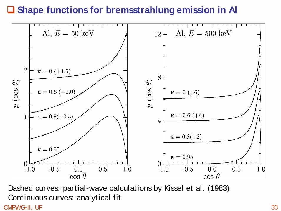
CMPWG-II, UF 33

Dashed curves: partial-wave calculations by Kissel et al. (1983)Continuous curves: analytical fit

Shape functions for bremsstrahlung emission in Al

CMPWG-II, UF 34

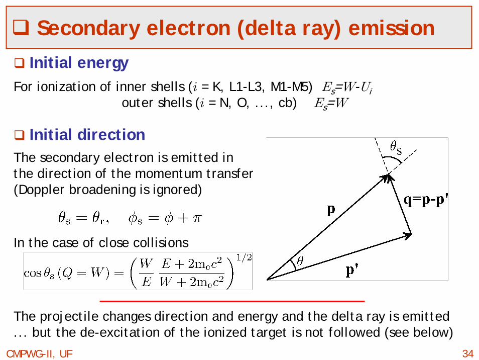
Secondary electron (delta ray) emissionInitial energy

For ionization of inner shells (i = K, L1-L3, M1-M5) Es=W-Uiouter shells (i = N, O, ..., cb) Es=W

The secondary electron is emitted in the direction of the momentum transfer (Doppler broadening is ignored)

In the case of close collisions

The projectile changes direction and energy and the delta ray is emitted... but the de-excitation of the ionized target is not followed (see below)

Initial direction

CMPWG-II, UF 35

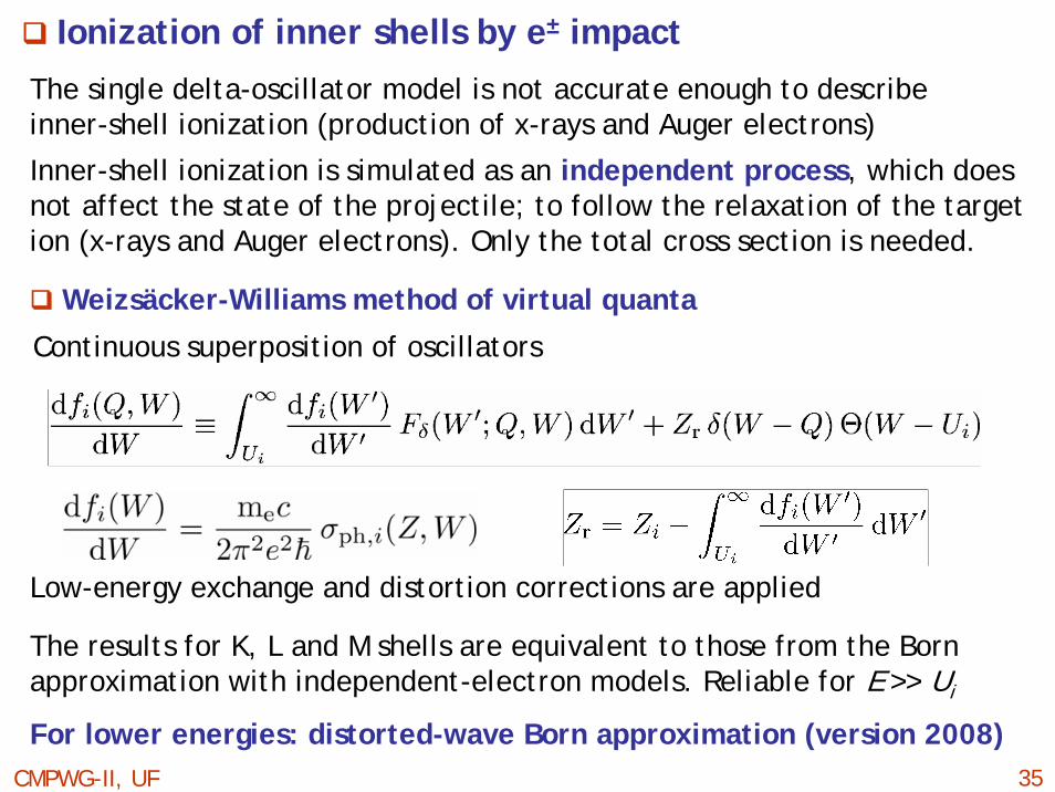
Ionization of inner shells by e± impactThe single delta-oscillator model is not accurate enough to describeinner-shell ionization (production of x-rays and Auger electrons)

Weizsäcker-Williams method of virtual quanta

Continuous superposition of oscillators

Low-energy exchange and distortion corrections are applied

The results for K, L and M shells are equivalent to those from the Born approximation with independent-electron models. Reliable for E >> Ui

For lower energies: distorted-wave Born approximation (version 2008)

Inner-shell ionization is simulated as an independent process, which does not affect the state of the projectile; to follow the relaxation of the target ion (x-rays and Auger electrons). Only the total cross section is needed.

CMPWG-II, UF 36

Continuous and dashed curves: WW method for electrons and positronsDots: First-principles Born approximation results of Scofield

Ionization cross sections by electron impact

CMPWG-II, UF 37

Positron annihilation

Heitler (two-photon) DCS The positron may annihilate either in flight or at rest

Continuous curves: in flightDashed curve: isotropic distribution

CMPWG-II, UF 38

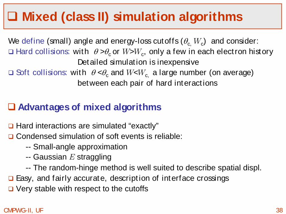
We define (small) angle and energy-loss cutoffs (θc, Wc) and consider:Hard collisions: with θ >θc or W>Wc, only a few in each electron history

Detailed simulation is inexpensiveSoft collisions: with θ <θc and W<Wc, a large number (on average)

between each pair of hard interactions

Hard interactions are simulated “exactly”Condensed simulation of soft events is reliable:

-- Small-angle approximation-- Gaussian E straggling -- The random-hinge method is well suited to describe spatial displ.

Easy, and fairly accurate, description of interface crossingsVery stable with respect to the cutoffs

Mixed (class II) simulation algorithms

Advantages of mixed algorithms

CMPWG-II, UF 39

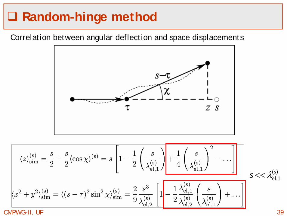
Random-hinge methodCorrelation between angular deflection and space displacements

(s)el,1 λ<<s

CMPWG-II, UF 40

Soft energy-loss events

Central-limit theorem

... but we must have ⇒

When this condition is not satisfied, we use “artificial” distributions withthe correct first and second moments

NOTES: 1) Consistent only when there are multiple soft events2) w is bound; w ≤ ⟨w⟩+ 3σ

... accurate only when w << E !

CMPWG-II, UF 41

Simulation parameters

0 ≤ C1 ≤ 0.2

0 ≤ C2 ≤ 0.2 (effective only at very high energies)

Wcc and Wcr (“estimated” from experiment/scoring details)

smax (to ensure multiple soft interactions,to allow energy-loss corrections,transport in EM fields)

When the input Wcr is negative, PENELOPE sets Wcr = 10 eV and soft bremsstrahlung is switched off

C1 = C2 = Wcc = smax = 0, Wcr = −10 eV ⇒ detailed simulation

CMPWG-II, UF 42

Stability

Example: 500 keV electrons in Al. s = 200 μm.

Detailed simulation C1 = C2 = 0; Wcc = 0 eVWcr = -100 eV (soft bremsstrahlung disregarded)

Mixed simulation CC11 = C2 = 0.2 (extreme case!)Wcc = 1 keV; Wcr = -100 eV (soft bremss. disregarded)smax = 20 μm

about 75 times faster

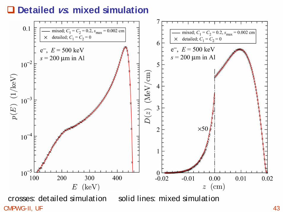
CMPWG-II, UF 43crosses: detailed simulation solid lines: mixed simulation

Detailed vs. mixed simulation

CMPWG-II, UF 44crosses: detailed simulation solid lines: mixed simulation

Detailed vs. mixed simulation

CMPWG-II, UF 45

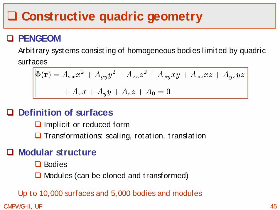
Constructive quadric geometry

PENGEOMArbitrary systems consisting of homogeneous bodies limited by quadric surfaces

Definition of surfacesImplicit or reduced formTransformations: scaling, rotation, translation

Modular structureBodiesModules (can be cloned and transformed)

Up to 10,000 surfaces and 5,000 bodies and modules

CMPWG-II, UF 46

Genealogical tree

modules (may have descendants, or not) bodies

To speed up the simulation, each module should have a small number ofdaughters (small number of branches in each node).Simulation speed is almost independent of the complexity of the geometry.

6

1

2

2

6

1

347

58

3

99

7 4

8

5

CMPWG-II, UF 47

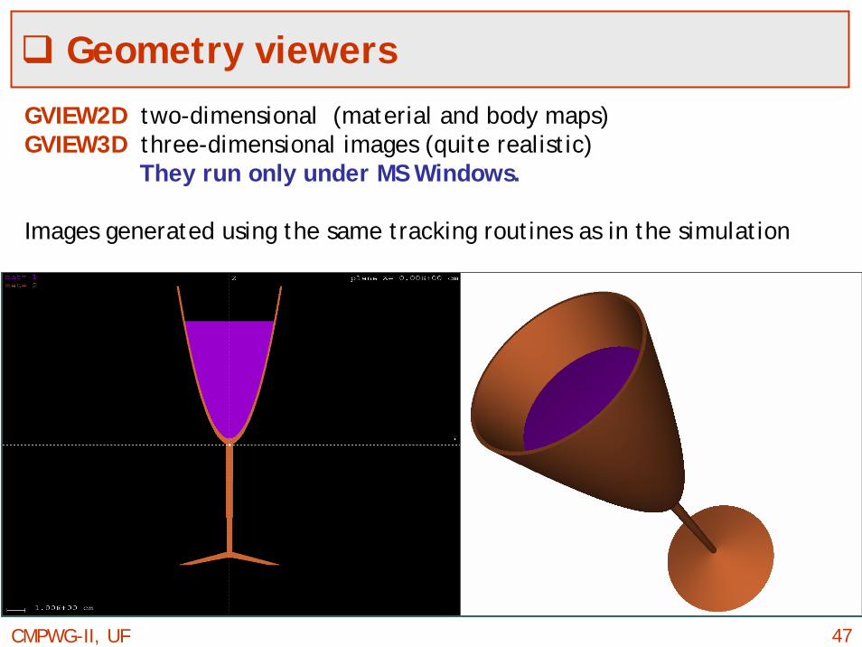
Geometry viewers

GVIEW2D two-dimensional (material and body maps)GVIEW3D three-dimensional images (quite realistic)

They run only under MS Windows.

Images generated using the same tracking routines as in the simulation

CMPWG-II, UF 48

Example: clinical electron accelerators

Varian 2300 C/D

CMPWG-II, UF 49

The subroutine package PENGEOM

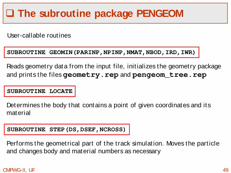
User-callable routines

SUBROUTINE GEOMIN(PARINP,NPINP,NMAT,NBOD,IRD,IWR)

Reads geometry data from the input file, initializes the geometry packageand prints the files geometry.rep and pengeom_tree.rep

SUBROUTINE LOCATE

Determines the body that contains a point of given coordinates and itsmaterial

SUBROUTINE STEP(DS,DSEF,NCROSS)

Performs the geometrical part of the track simulation. Moves the particleand changes body and material numbers as necessary

CMPWG-II, UF 50

SUBROUTINE STEP does not stop particles when they cross an interface between adjacent bodies of the same composition. That is, these interfaces are not visible from the main program

COMMON/QKDET/KDET(NB)

KDET(KB)is initialised to zero. Body KB is made part of impact detector IDET by setting KDET(KB)=IDET (in main program). When particles enter body KB coming from a body that is not part of detector IDET, they are halted at the surface of the active body and control is returned to the main program.

Thus, detector surfaces are made visible from the main program.

Impact detectors are useful for visualising bodies (GVIEW2D), for simulating real detectors and for generating phase-space files (PENMAIN).

Impact detectors

CMPWG-II, UF 51

Structure of the main program

main program

PENELOPE PENGEOM PENVARED TIMER

The communication between the main program and the simulation routinesis through a few common blocks

PENELOPE is a set of Fortran subroutine packages. The user must provide a steering main program that generates the initial states of primary particles, controls the evolution of the simulated tracks and keeps score of relevant quantities.

NOTE: the generic main program penmain can handle a wide variety of problems, but yours may require some special treatment ...

CMPWG-II, UF 52

COMMON/TRACK/E,X,Y,Z,U,V,W,WGHT,KPAR,IBODY,MAT,ILB(5)

KPAR ... kind of particle (1=electron, 2=photon, 3=positron)E ... current particle's energy (eV)X,Y,Z ... position coordinates (cm)U,V,W ... direction cosinesWGHT ... particle's weight (used only with variance reduction) IBODY ... index of body where the particle is moving MAT ... corresponding materialILB(5)... describes origin of secondary particles (pp. 215-216)

Most of the information flux between the main program and the simulationand geometry subroutines is through the common block

which contains the following quantities:

To start the simulation of a particle, its initial state variables must be set bythe main program. PENELOPE modifies the energy and direction cosines only when the particle undergoes an interaction. The position coordinatesare updated by PENGEOM.

In the I/O of the PENELOPE and PENGEOM routines, all energiesare in eV and all lengths are in cm

CMPWG-II, UF 53

The PENELOPE subroutines

SUBROUTINE CLEANS

SUBROUTINE START

SUBROUTINE JUMP(DSMAX,DS)

SUBROUTINE KNOCK(DE,ICOL)

SUBROUTINE SECPAR(LEFT)

SUBROUTINE STORES(E,X,Y,Z,U,V,W,WGHT,KPAR,ILB)

Initializes the secondary stack

Starts a new shower

generate particle histories

gets secondary particles from the stack

stores particles in the stack (splitting)

SUBROUTINE PEINIT(EPMAX,NMAT,IRD,IWR,INFO)

CMPWG-II, UF 54

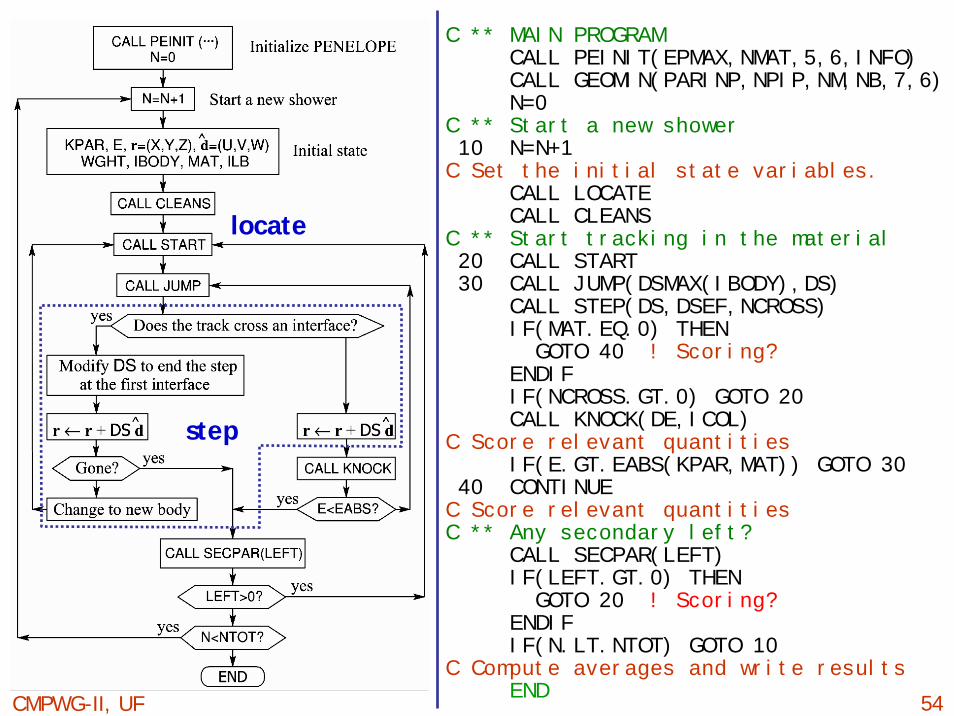
C ** MAIN PROGRAMCALL PEINIT(EPMAX,NMAT,5,6,INFO) CALL GEOMIN(PARINP,NPIP,NM,NB,7,6) N=0

C ** Start a new shower10 N=N+1

C Set the initial state variables.CALL LOCATE CALL CLEANS

C ** Start tracking in the material20 CALL START 30 CALL JUMP(DSMAX(IBODY),DS)

CALL STEP(DS,DSEF,NCROSS) IF(MAT.EQ.0) THEN GOTO 40 ! Scoring?

ENDIFIF(NCROSS.GT.0) GOTO 20CALL KNOCK(DE,ICOL)

C Score relevant quantitiesIF(E.GT.EABS(KPAR,MAT)) GOTO 30

40 CONTINUEC Score relevant quantitiesC ** Any secondary left?

CALL SECPAR(LEFT)IF(LEFT.GT.0) THENGOTO 20 ! Scoring?

ENDIFIF(N.LT.NTOT) GOTO 10

C Compute averages and write resultsEND

locate

step

CMPWG-II, UF 55

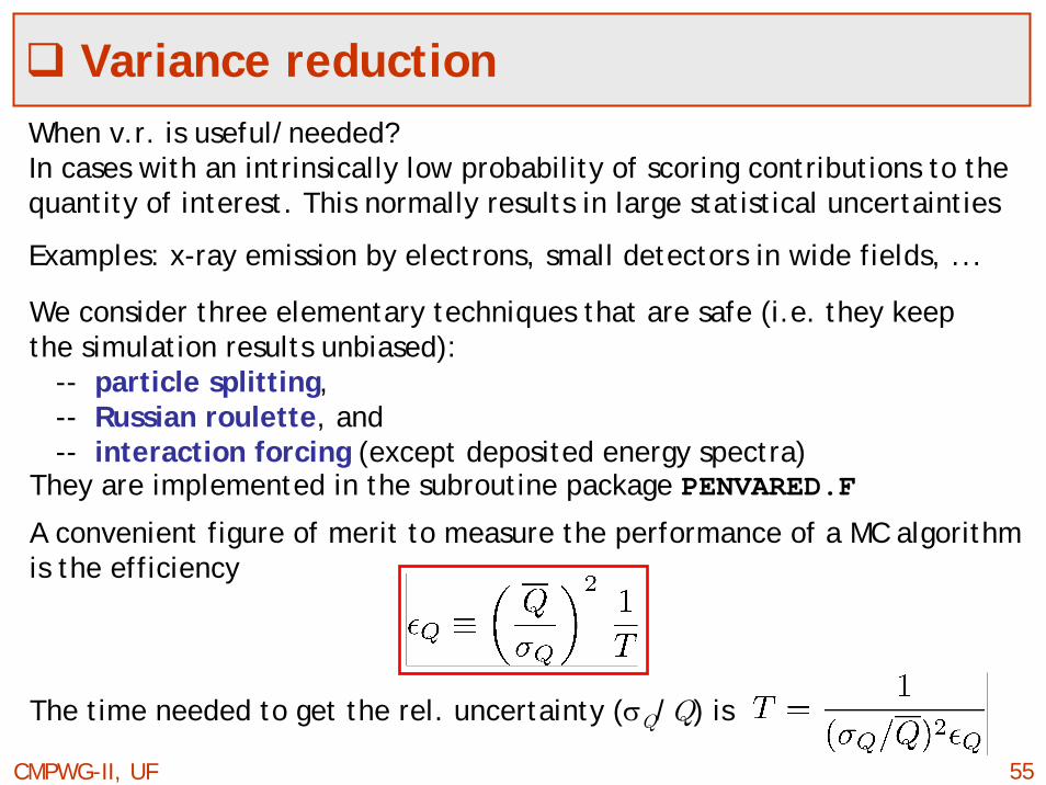
Variance reduction

We consider three elementary techniques that are safe (i.e. they keep the simulation results unbiased):

-- particle splitting, -- Russian roulette, and -- interaction forcing (except deposited energy spectra)

They are implemented in the subroutine package PENVARED.F

When v.r. is useful/needed?In cases with an intrinsically low probability of scoring contributions to the quantity of interest. This normally results in large statistical uncertainties

Examples: x-ray emission by electrons, small detectors in wide fields, ...

A convenient figure of merit to measure the performance of a MC algorithm is the efficiency

The time needed to get the rel. uncertainty (σQ/Q) is

CMPWG-II, UF 56

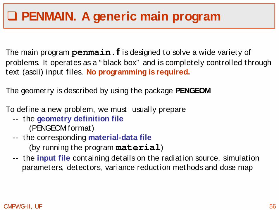
PENMAIN. A generic main program

The main program penmain.f is designed to solve a wide variety of problems. It operates as a “black box” and is completely controlled throughtext (ascii) input files. No programming is required.

The geometry is described by using the package PENGEOM

To define a new problem, we must usually prepare -- the geometry definition file

(PENGEOM format)-- the corresponding material-data file

(by running the program material)-- the input file containing details on the radiation source, simulation

parameters, detectors, variance reduction methods and dose map

CMPWG-II, UF 57

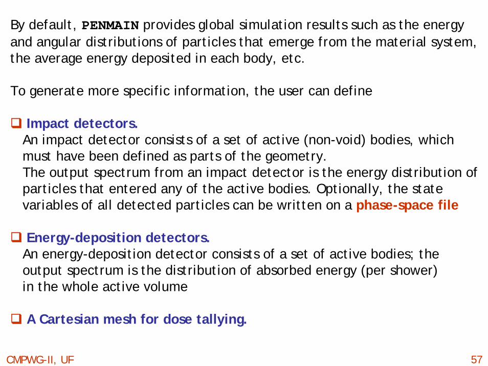
By default, PENMAIN provides global simulation results such as the energy and angular distributions of particles that emerge from the material system,the average energy deposited in each body, etc.

To generate more specific information, the user can define

Impact detectors.An impact detector consists of a set of active (non-void) bodies, which must have been defined as parts of the geometry. The output spectrum from an impact detector is the energy distribution of particles that entered any of the active bodies. Optionally, the state variables of all detected particles can be written on a phase-space file

Energy-deposition detectors.An energy-deposition detector consists of a set of active bodies; theoutput spectrum is the distribution of absorbed energy (per shower)in the whole active volume

A Cartesian mesh for dose tallying.

CMPWG-II, UF 58

Structure of the input file

....+....1....+....2....+....3....+....4....+....5....+....6....+....TITLE Title of the job, up to 120 characters.

>>>>>>>> Source definition. SKPAR KPARP [Primary particles: 1=electron, 2=photon, 3=positron]SENERG SE0 [Initial energy (monoenergetic sources only)]SPECTR Ei,Pi [E bin: lower-end and total probability]SPOSIT SX0,SY0,SZ0 [Coordinates of the source]SDIREC STHETA,SPHI [Beam axis direction angles, in deg]SAPERT SALPHA [Beam aperture, in deg]

>>>>>>>> Input phase-space file (psf). IPSFN psf_filename.ext [Input psf name, 20 characters]IPSPLI NSPLIT [Splitting number]EPMAX EPMAX [Maximum energy of particles in the psf]

>>>>>>>> Material data and simulation parameters. NMAT NMAT [Number of different materials, .le.10]SIMPAR M,EABS(1:3,M),C1,C2,WCC,WCR [Sim. parameters for material M]PFNAME mat_filename.ext [Material definition file, 20 chars]

>>>>>>>> Geometry definition file. GEOMFN geo_filename.ext [Geometry definition file, 20 chars]DSMAX IBODY,DSMAX(IBODY) [IB, maximum step length (cm) in body IB]

....+....1....+....2....+....3....+....4....+....5....+....6....+....

CMPWG-II, UF 59

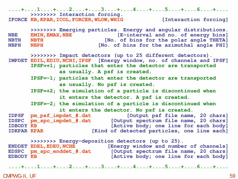
....+....1....+....2....+....3....+....4....+....5....+....6....+....>>>>>>>> Interaction forcing.

IFORCE KB,KPAR,ICOL,FORCER,WLOW,WHIG [Interaction forcing]

>>>>>>>> Emerging particles. Energy and angular distributions. NBE EMIN,EMAX,NBE [E-interval and no. of energy bins] NBTH NBTH [No. of bins for the polar angle THETA] NBPH NBPH [No. of bins for the azimuthal angle PHI]

>>>>>>>> Impact detectors (up to 25 different detectors).IMPDET EDIL,EDIU,NCHI,IPSF [Energy window, no. of channels and IPSF]

IPSF=+1; particles that enter the detector are transportedas usually. A psf is created.

IPSF=-1; particles that enter the detector are transportedas usually. No psf is created.

IPSF=+2; the simulation of a particle is discontinued whenit enters the detector. A psf is created.

IPSF=-2; the simulation of a particle is discontinued whenit enters the detector. No psf is created.

IDPSF pm_psf_impdet_#.dat [Output psf file name, 20 chars] IDSPC pm_spc_impdet_#.dat [Output spectrum file name, 20 chars] IDBODY KB [Active body; one line for each body] IDKPAR KPAR [Kind of detected particles, one line each]

>>>>>>>> Energy-deposition detectors (up to 25). ENDDET EDEL,EDEU,NCHE [Energy window and number of channels] EDSPC pm_spc_enddet_#.dat [Output spectrum file name, 20 chars] EDBODY KB [Active body; one line for each body]

....+....1....+....2....+....3....+....4....+....5....+....6....+....

CMPWG-II, UF 60

....+....1....+....2....+....3....+....4....+....5....+....6....+....

>>>>>>>> Dose distribution. GRIDX XL,XU [X coordinates of the enclosure vertices] GRIDY YL,YU [Y coordinates of the enclosure vertices] GRIDZ ZL,ZU [Z coordinates of the enclosure vertices] GRIDBN NX,NY,NZ [Numbers of bins]

>>>>>>>> Job properties RESUME pm_dumpfile_1.dat [Resume from this dump file, 20 chars] DUMPTO pm_dumpfile_2.dat [Generate this dump file, 20 chars] DUMPP DUMPP [Dumping period, in sec]

NSIMSH NTOT [Desired number of simulated showers] RSEED ISEED1,ISEED2 [Seeds of the random number generator] TIME TIMEA [Allotted simulation time, in sec] ....+....1....+....2....+....3....+....4....+....5....+....6....+....

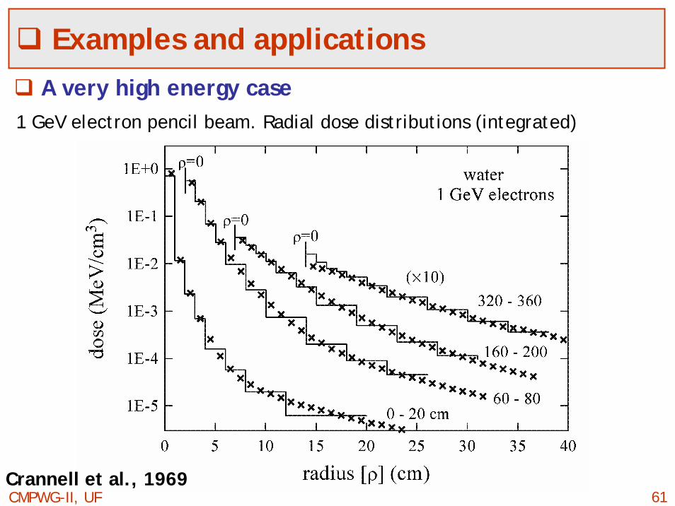
CMPWG-II, UF 61Crannell et al., 1969

1 GeV electron pencil beam. Radial dose distributions (integrated)

A very high energy case

Examples and applications

CMPWG-II, UF 62Werner et al., 1988

keV electron beams. Depth-dose distributions... and a low-energy case

CMPWG-II, UF 63

Siemens KDS electron accelerator

CMPWG-II, UF 64

32P source wire for intravascular brachytherapy

CMPWG-II, UF 65

32P source wirein water

CMPWG-II, UF 66

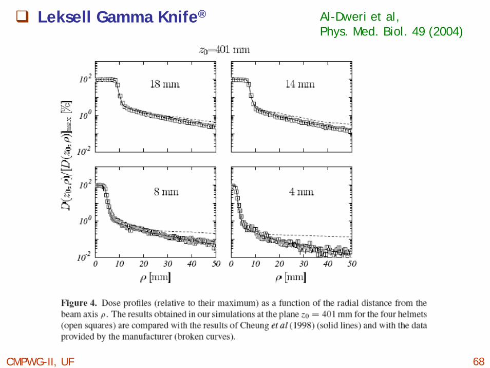
Leksell Gamma Knife®

Al-Dweri et al, Phys. Med. Biol. 49 (2004)

CMPWG-II, UF 67

CMPWG-II, UF 68

Leksell Gamma Knife® Al-Dweri et al, Phys. Med. Biol. 49 (2004)

CMPWG-II, UF 69

p-type HP Ge detector, Marinelli beaker (García-Toraño, NIMA 2005).

simulated (penelope)

measured

Gamma-ray spectrometry

CMPWG-II, UF 70

not affected by coincidences affected by coincidence-summingsimulation (PENELOPE)

Gamma-ray spectrometry. Detection efficiencies

CMPWG-II, UF 71

The electron microprobe

5 keV ≤ E ≤ 45 keVHighly stableAccurate positioningAbsolute spectra

X-ray microanalysis

e−γ

CMPWG-II, UF 72

X-ray microanalysis. Simulation geometry.

CMPWG-II, UF 73

X-ray absolute spectra

CMPWG-II, UF 74

X-ray absolute spectra

CMPWG-II, UF 75

Work in progress

Inner shell ionization by electron and positron impact(Distorted-wave Born approximation)

Re-evaluation of the density effect on the stopping power(effective oscillator strengths of individual shells)

Photon polarization

Adaptive variance reduction (ant-colony method)

... and other practical improvements requested by users