1

Tractable Model for Rate in Self-BackhauledMillimeter Wave Cellular Networks

Sarabjot Singh, Mandar N. Kulkarni, Amitava Ghosh, and Jeffrey G. Andrews

Abstract—Millimeter wave (mmW) cellular systems will re-quire high gain directional antennas and dense base station(BS) deployments to overcome high near field path loss andpoor diffraction. As a desirable side effect, high gain antennasprovide interference isolation, providing an opportunity to in-corporate self-backhauling–BSs backhauling among themselvesin a mesh architecture without significant loss in throughput–toenable the requisite large BS densities. The use of directionalantennas and resource sharing between access and backhaullinks leads to coverage and rate trends that differ significantlyfrom conventional microwave (µW) cellular systems. In thispaper, we propose a general and tractable mmW cellular modelcapturing these key trends and characterize the associated ratedistribution. The developed model and analysis is validatedusing actual building locations from dense urban settings andempirically-derived path loss models. The analysis shows that insharp contrast to the interference limited nature of µW cellularnetworks, the spectral efficiency of mmW networks (besides totalrate) also increases with BS density particularly at the cell edge.Increasing the system bandwidth, although boosting median andpeak rates, does not significantly influence the cell edge rate. Withself-backhauling, different combinations of the wired backhaulfraction (i.e. the faction of BSs with a wired connection) and BSdensity are shown to guarantee the same median rate (QoS).

I. INTRODUCTION

The scarcity of “beachfront” microwave spectrum [1] andsurging wireless traffic demands has made going higher in fre-quency for terrestrial communications inevitable. The capacityboost provided by increased LTE deployments and aggressivesmall cell, particularly Wi-Fi, offloading has, so far, been ableto cater to the increasing traffic demands, but to meet theprojected [2] traffic needs of 2020 (and beyond) availabilityof large amounts of new spectrum would be indispensable. Theonly place where a significant amount of unused or lightly usedspectrum is available is in the millimeter wave (mmW) bands(20− 100 GHz). With many GHz of spectrum to offer, mmWbands are becoming increasingly attractive as one of the frontrunners for the next generation (a.k.a. “5G”) wireless cellularnetworks [3]–[5].

A. Background and recent work

Feasibility of mmW cellular. Although mmW based indoorand personal area networks have already received considerabletraction [6], [7], such frequencies have long been deemedunattractive for cellular communications primarily due to the

This work has been supported by Nokia. S. Singh, M. N. Kulkarni,and J. G. Andrews are with Wireless Networking and CommunicationsGroup (WNCG), The University of Texas at Austin and A. Ghosh iswith Nokia (email: sarabjot@utexas.edu, kulkarni.mandar.n@gmail.com, ami-tava.ghosh@nsn.com, and jandrews@ece.utexas.edu).

large near-field loss and poor penetration (blocking) throughconcrete, water, foliage, and other common material. Recentresearch efforts [4], [8]–[14] have, however, seriously chal-lenged this widespread perception. In principle, the smallerwavelengths associated with mmW allow placing many moreminiaturized antennas in the same physical area, thus com-pensating for the near-field path loss [8], [9]. Communicationranges of 150-200m have been shown to be feasible in denseurban scenarios with the use of such high gain directionalantennas [4], [9], [10]. Although mmW signals do indeedpenetrate and diffract poorly through urban clutter, dense urbanenvironments offer rich multipath (at least for outdoor) withstrong reflections; making non-line-of-sight (NLOS) commu-nication feasible with familiar path loss exponents in the rangeof 3-4 [4], [9]. Dense and directional mmW networks havebeen shown to exhibit a similar spectral efficiency to 4G(LTE) networks (of the same density) [11], [12], and hencecan achieve an order of magnitude gain in throughput due tothe increased bandwidth.

Coverage trends in mmW cellular. With high gain direc-tional antennas and newfound sensitivity to blocking, mmWcoverage trends will be quite different from previous cellularnetworks. Investigations via detailed system level simulations[11]–[15] have shown large bandwidth mmW networks inurban settings1 tend to be noise limited–i.e. thermal noise dom-inates interference–in contrast to 4G cellular networks, whichare usually strongly interference limited. As a result, mmWoutages are mostly due to a low signal-to-noise-ratio (SNR)instead of low signal-to-interference-ratio (SIR). This insightwas also highlighted in an earlier work [16] for directionalmmW ad hoc networks. Because cell edge users experiencelow SNR and are power limited, increased bandwidth leadsto little or no gain in their rates as compared to the medianor peak rates [12]. Note that rates were compared with a 4Gnetwork in [12], however, in this paper we also investigateeffect of bandwidth on rate in mmW regime.

Density and backhaul. As highlighted in [8], [11]–[15],dense BS deployments are essential for mmW networks toachieve acceptable coverage and rate. This poses a particularchallenge for the backhaul network, especially given thehuge rates stemming from mmW bandwidths on the order ofGHz. However, the interference isolation provided by narrowdirectional beams provides a unique opportunity for organicand scalable backhaul architectures [8], [17], [18]. Specifically,self-backhauling is a natural and scalable solution [17]–[19],

1Note that capacity crunch is also most severe in such dense urbanscenarios.

arX

iv:1

407.

5537

v1 [

cs.I

T]

21

Jul 2

014

2

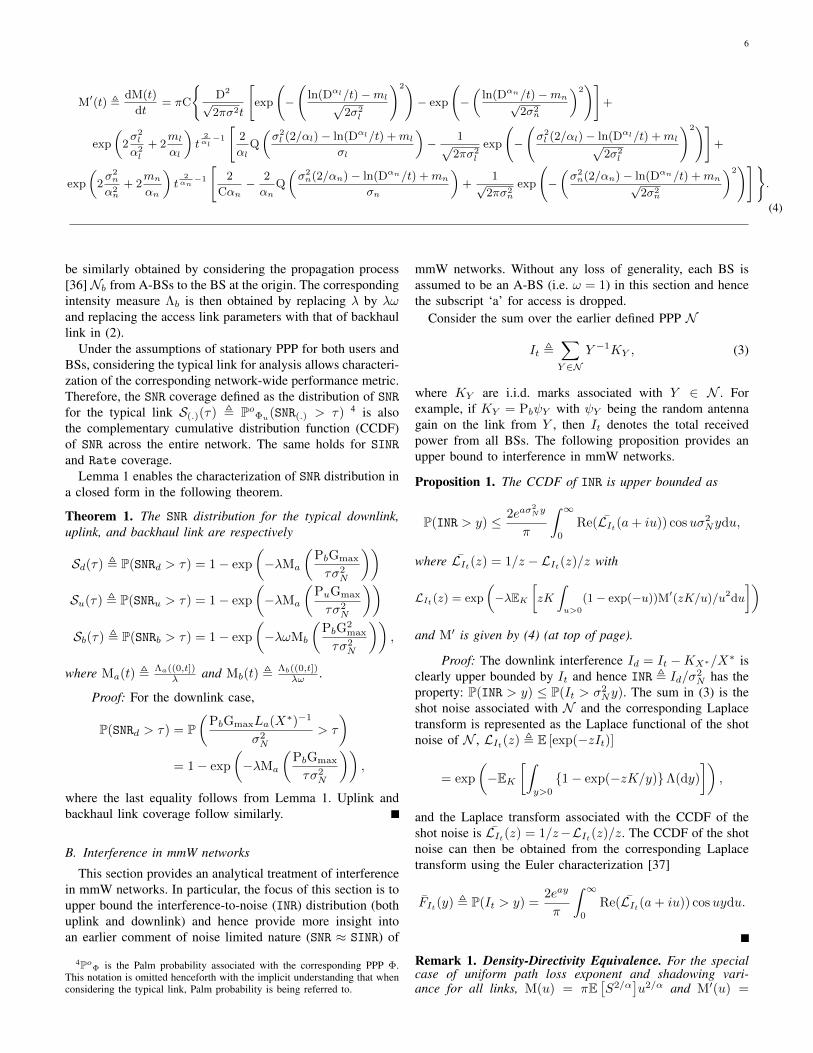
where BSs with wired backhaul provide for the backhaul ofBSs without it using a mmW link. This architecture is quitedifferent from the mmW based point-to-point backhaul [20]or the relaying architecture [21] already in use, as (a) the BSwith wired backhaul serves multiple BSs, and (b) access andbackhaul link share the total pool of available resources ateach BS. This results in a multihop network, but one in whichthe hops need not interfere, which is what largely doomedprevious attempts at mesh networking. However, both the loadon the backhaul and access link impact the eventual userrate, and a general and tractable model that integrates thebackhauling architecture into the analysis of a mmW cellularnetwork seems important to develop. The main objective ofthis work is to address this. As we show, the very notionof a coverage/association cell is strongly questionable due tothe sensitivity of mmW to blocking in dense urban scenarios.Characterizing the load and rate in such networks, therefore,is non-trivial due to the formation of irregular and “chaotic”association cells (see Fig. 3).

Relevant models. Recent work in developing models forthe analysis of mmW cellular networks (ignoring backhaul)includes [22]–[24], where the downlink SINR distribution ischaracterized assuming BSs to be spatially distributed accord-ing to a Poisson point process (PPP). No blockages wereassumed in [22], while [23] proposed a line of sight (LOS)ball based blockage model in which all nearby BSs wereassumed LOS and all BSs beyond a certain distance from theuser were ignored. This blockage model can be interpretedas a step function approximation of the exponential blockagemodel proposed in [25] and used in [24]. Coverage was shown[23] to improve with antenna directionality, and to exhibit anon-monotonic trend with BS density. In this work, however,we show that if the finite user population is taken into account(ignored in [23]), SINR coverage increases monotonically withdensity. Although characterizing SINR is important, rate isthe key metric, and can follow quite different trends [26],[27] than SINR because the user load is essentially a pre-llogfactor whereas SINR is inside the log in the Shannon capacityformula.

B. Contributions

The major contributions of this paper can be categorizedbroadly as follows:Tractable mmW cellular model. A tractable and generalmodel is proposed in Sec. II for characterizing uplink anddownlink coverage and rate distribution in self-backhauledmmW cellular networks. The proposed blockage model allowsfor an adaptive fraction of area around each user to be LOS.Assuming the BSs are distributed according to a PPP, theanalysis, developed in Sec. III, accounts for different pathlosses (both mean and variance) of LOS/NLOS links for bothaccess and backhaul–consistent with empirical studies [4],[14]. We identify and characterize two types of associationcells in self-backhauled networks: (a) user association areaof a BS which impacts the load on the access link, and (b) BSassociation area of a BS with wired backhaul required forquantifying the load on the backhaul link. The rate distribution

across the entire network, accounting for the random backhauland access link capacity, is then characterized in Sec III.Further, the analysis is extended to derive the rate distributionwith offloading to and from a co-existing µW macrocellularnetwork.Validation of model and analysis. In Sec. III-E, the analyticalrate distribution derived from the proposed model is comparedwith that obtained from simulations employing actual buildinglocations in dense urban regions of New York [28] andChicago [29], and empirically measured path loss models[14]. The demonstrated close match between the analysis andsimulation validates the proposed blockage model and ouranalytical approximation of the irregular association areas andload.Performance insights. Using the developed framework, it isdemonstrated in Sec. IV that:• MmW networks in dense urban scenarios employing high

gain narrow beam antennas tend to be noise limited for“practical” BS densities. Consequently, densification ofthe network improves the SINR coverage, especially foruplink. Incorporating the impact of finite user density,SINR coverage is shown to monotonically increase withdensity even in the very large density regime.

• Cell edge users experience poor SNR and hence areparticularly power limited. Increasing the air interfacebandwidth, as a result, does not significantly improvethe cell edge rate, in contrast to the cell median or peakrates. Improving the density, however, improves the celledge rate drastically. Assuming all users to be mmWcapable, cell edge rates are also shown to improve byreverting users to the µW network whenever reliablemmW communication is unfeasible.

• Self-backhauling is attractive due to the diminished effectof interference in such networks. Increasing the fractionof BSs with wired backhaul, obviously, improves the peakrates in the network. Increasing the density of BSs whilekeeping the density of wired backhaul BSs constant in thenetwork, however, leads to saturation of user rate cover-age. We characterize the corresponding saturation densityas the BS density beyond which marginal improvementin rate coverage would be observed without further wiredbackhaul provisioning. The saturation density is shownto be proportional to the density of BSs with wiredbackhaul.

• The same rate coverage/median rate is shown to beachievable with various combinations of (i) the fractionof wired backhaul BSs and (ii) the density of BSs. A rate-density-backhaul contour is characterized, which shows,for example, that the same median rate can be achievedthrough a higher fraction of wired backhaul BSs in sparsenetworks or a lower fraction of wired backhaul BSs indense deployments.

II. SYSTEM MODEL

A. Spatial locations

The mmW BSs in the network are assumed to be distributeduniformly in R2 as an homogeneous PPP Φ of density (inten-

3

sity) λ. The PPP assumption is taken for tractability, howeverother spatial models can be expected to exhibit similar trendsdue to the nearly constant SINR gap over that of the PPP[30]. The users are also assumed to be uniformly distributedas a PPP Φu of density (intensity) λu in R2. A fraction ωof the BSs (called anchored BS or A-BS henceforth) havewired backhaul and the rest of BSs backhaul wirelessly to A-BSs. So, the A-BSs serve the rest of the BSs in the networkresulting in two-hop links to the users associated with the BSs.Independent marking assigns wired backhaul (or not) to eachBS and hence the resulting independent point process of A-BSs Φw is also a PPP with density λω. A fraction µ

λ (assignedby independent marking) of the BSs are assumed to form theµW macrocellular network and thus the corresponding PPPΦµ is of density µ.

Notation is summarized in Table I. Capital roman font isused for parameters and italics for random variables.

B. Propagation assumptions

For mmW transmission, the power received at y ∈ R2

from a transmitter at x ∈ R2 transmitting with power P(x)is given by P(x)ψ(x, y)L(x, y)−1, where ψ is the combinedantenna gain of the receiver and transmitter and L (dB)=β + 10α log10 ‖x− y‖+ χ is the associated path loss in dB,where χ ∼ N (0, ξ2). Different strategies can be adopted forformulating the path loss model from field measurements. Ifβ is constrained to be the path loss at a close-in referencedistance, then α is physically interpreted as the path lossexponent. But if these parameters are obtained by a best linearfit, then β is the intercept and α is the slope of the fit, andno physical interpretation may be ascribed. The deviation infitting (in dB scale) is modeled as a zero mean Gaussian(Lognormal in linear scale) random variable χ with varianceξ2. Motivated by the studies in [4], [14], which point todifferent LOS and NLOS path loss parameters for access (BS-user) and backhaul (BS-A-BS) links, the analytical model inthis paper accommodates distinct β, α, and ξ2 for each. EachmmW BS and user is assumed to transmit with power Pb andPu, respectively, over a bandwidth B. The transmit power andbandwidth for µW BS is denoted by Pµ and Bµ respectively.

All mmW BSs are assumed to be equipped with directionalantennas with a sectorized gain pattern. Antenna gain patternfor a BS as a function of angle θ about the steering angle isgiven by

Gb(θ) =

{Gmax if |θ| ≤ θbGmin otherwise.

,

where θb is the beam-width or main lobe width. Similarabstractions have been used in the prior study of directional adhoc networks [31], cellular networks [32], and recently mmWnetworks [22], [23]. The user antenna gain pattern Gu(θ) canbe modeled in the same manner; however, in this paper weassume omnidirectional antennas for the users. The beams ofall non-intended links are assumed to be randomly orientedwith respect to each other and hence the effective antennagains (denoted by ψ) on the interfering links are random. Theantennas beams of the intended access and backhaul link are

TABLE I: Notation and simulation parameters

Nota-tion

Parameter Value (if applicable)

Φ, λ mmW BS PPP and densityω Anchor BS (A-BS) fraction

Φu, λu user PPP and density λu = 1000 per sq. kmΦµ, µ µW BS PPP and density µ = 5 per sq. km

B mmW bandwidth 2 GHzBµ µW bandwidth 20 MHzPb mmW BS transmit power 30 dBmPu user transmit power 20 dBmξ standard deviation of path loss Access: LOS = 4.9,

NLOS = 7.6Backhaul: LOS = 4.1,NLOS = 7.9

α path loss exponent Access: LOS = 2.1,NLOS = 3.3Backhaul: LOS = 2,NLOS = 3.5 [14]

ν mmW carrier frequency 73 GHzβ path loss at 1 m 70 dB

Gmax,Gmin,θb

main lobe gain, side lobegain, beam-width

Gmax = 18 dB,Gmin = −2 dB,θb = 10o

C,D fractional LOS area C incorresponding ball of radiusD

0.12, 200 m

σ2N noise power thermal noise power plus

noise figure of 10 dB

assumed to be aligned, i.e., the effective gain on the desiredaccess link is Gmax and on the desired backhaul link is G2

max.Analyzing the impact of alignment errors on the desired linkis beyond the scope of the current work, but can be done onthe lines of the recent work [33]. It is worth pointing out herethat since our analysis is restricted to 2-D, the directivity of theantennas is modeled only in the azimuthal plane, whereas inpractice due to the 3-D antenna gain pattern [9], [14], the RFisolation to the unintended receivers would also be providedby differences in elevation angles.

C. Blockage model

Each access link of separation d is assumed to be LOSwith probability C if d ≤ D and 0 otherwise2. The parameterC should be physically interpreted as the average fraction ofLOS area in a circular ball of radius D around the point underconsideration. The proposed approach is simple yet flexibleenough to capture blockage statistics of real settings as shownin Sec. III-E. The insights presented in this paper corroboratethose from other blockage models too [12], [14], [23]. Theparameters (C,D) are geography and deployment dependent(low for dense urban, high for semi-urban). The analysis inthis paper allows for different (C, D) pairs for access andbackhaul links.

D. Association rule

Users are assumed to be associated (or served) by the BSoffering the minimum path loss. Therefore, the BS servingthe user at origin is X∗(0) , arg minX∈Φ La(X, 0), where‘a’ (‘b’) is for access (backhaul). The index 0 is dropped

2A fix LOS probability beyond distance D can also be handled as shownin Appendix A.

4

Rate =

B

Nu,w+κNblog(1 + SINRa) if associated with an A-BS,

BNu

min((

1− κκNb+Nu,w

)log(1 + SINRa), κ

κNb+Nu,wlog(1 + SINRb)

)otherwise.

(1)

Wireless backhaul

Access links

A-BS

BS

BS

BS

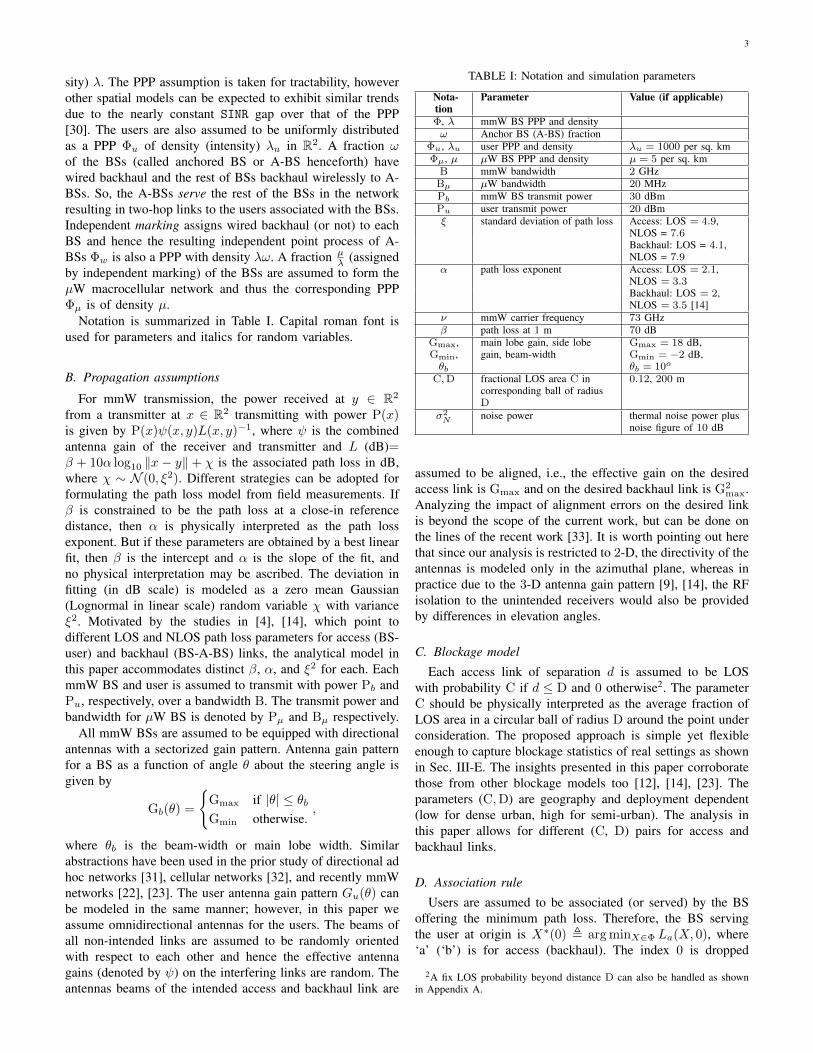
Fig. 1: Self-backhauled network with the A-BS providing thewireless backhaul to the associated BSs and access link to theassociated users (denoted by circles). The solid lines depict theregions in which all BSs are served by the A-BS at the center.

henceforth wherever implicit. The analysis in this paper isdone for the user located at the origin referred to as the typicaluser3 and its serving BS is the tagged BS. Further, each BS(with no wired backhaul) is assumed to be backhauled overthe air to the A-BS offering the lowest path loss to it. Thus,the A-BS (tagged A-BS) serving the tagged BS at X∗ (if notan A-BS itself) is Y ∗(X∗) , arg minY ∈Φw Lb(Y,X

∗), withX∗ /∈ Φw. This two-hop setup is demonstrated in Fig. 1. Asa result, the access (downlink and uplink), and backhaul linkSINR are

SINRd =PbGmaxLa(X∗)−1

Id + σ2N

, SINRu =PuGmaxLa(X∗)−1

Iu + σ2N

,

SINRb =PbG

2maxLb(X

∗, Y ∗)−1

Ib + σ2N

,

respectively, where σ2N , N0B is the thermal noise power and

I(.) is the corresponding interference.

E. Validation methodology

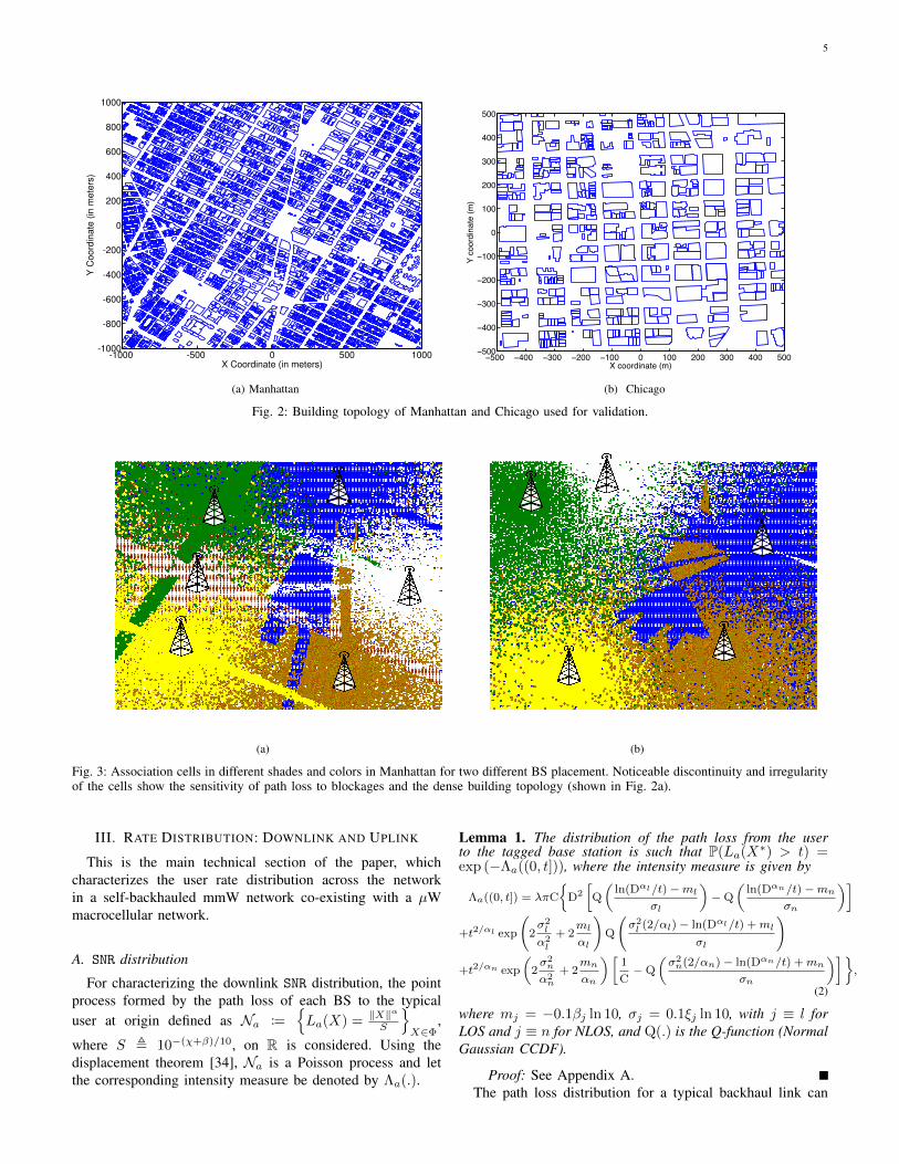
The analytical model and results presented in this paperare validated using Monte Carlo simulations employing actualbuilding topology of two major metropolitan areas, Manhat-tan and Chicago, obtained from [28] and [29] respectively.The polygons representing the buildings in the correspondingregions are shown in Fig. 2. These regions represent denseurban settings, where mmW networks are most attractive. Ineach simulation trial, users and BSs are dropped randomly inthese geographical areas as per the corresponding densities.

3Notion of typicality is enabled by Slivnyak’s theorem [34].

Users are dropped only in the outdoor regions, whereas theBSs landing inside a building polygon are assumed to beNLOS to all users. A BS-user link is assumed to be NLOS ifa building blocks the line segment joining the two, and LOSotherwise. The association and propagation rules are assumedas described in the earlier sections. The specific path lossparameters used are listed in Table I and are from empiricalmeasurements [14]. The association cells formed by twodifferent placements of mmW BSs in downtown Manhattanwith this methodology are shown in Fig. 3.

F. Access and backhaul load

Access and backhaul links are assumed to share the samepool of radio resources and hence the user rate depends onthe user load at BSs and BS load at A-BSs. Let Nb, Nu,w,and Nu denote the number of BSs associated with the taggedA-BS, number of users served by the tagged A-BS, and thenumber of users associated with the tagged BS respectively.By definition, when the typical user associates with an A-BS,Nu,w = Nu. Since an A-BS serves both users and BSs, theresources allocated to the associated BSs (which further servetheir associated users) are assumed to be proportional to theiraverage user load. Let the average number of users per BS bedenoted by κ , λu/λ, and then the fraction of resources ηbavailable for all the associated BSs at an A-BS are κNb

κNb+Nu,w,

and those for the access link with the associated users are thenηa,w = 1−ηb =

Nu,wκNb+Nu,w

. The fraction of resources reservedfor the associated BSs at an A-BS are assumed to be sharedequally among the BSs and hence the fraction of resourcesavailable to the tagged BS from the tagged A-BS are ηb/Nb,which is equivalent to the resource fraction used for backhaulby the corresponding BS. The access and backhaul capacity ateach BS is assumed to be shared equally among the associatedusers.

With the above described resource allocation model therate/throughput of a user is given by (1) (at top of this page),where SINRa corresponds to the SINR of the access link: a ≡ dfor downlink and a ≡ u for uplink.

G. Hybrid networks

Co-existence with conventional µW based 3G and 4Gnetworks could play a key role in providing wide coverage,particularly in sparse deployment of mmW networks, andreliable control channels. In this paper, a simple offloadingtechnique is adopted wherein a user is offloaded to the µWnetwork if it’s SINR on the mmW network drops below athreshold τmin. Although an SINR based offloading strategyis highly suboptimal for µW HetNets [27], due to the largebandwidth disparity between the mmW and µW network it isarguably reasonable in mmW [26], [35].

5

-1000 -500 0 500 1000-1000

-800

-600

-400

-200

0

200

400

600

800

1000

X Coordinate (in meters)

Y C

oo

rdin

ate

(in

me

ters

)

(a) Manhattan

−500 −400 −300 −200 −100 0 100 200 300 400 500−500

−400

−300

−200

−100

0

100

200

300

400

500

X coordinate (m)

Y co

ordi

nate

(m)

(b) Chicago

Fig. 2: Building topology of Manhattan and Chicago used for validation.

(a) (b)

Fig. 3: Association cells in different shades and colors in Manhattan for two different BS placement. Noticeable discontinuity and irregularityof the cells show the sensitivity of path loss to blockages and the dense building topology (shown in Fig. 2a).

III. RATE DISTRIBUTION: DOWNLINK AND UPLINK

This is the main technical section of the paper, whichcharacterizes the user rate distribution across the networkin a self-backhauled mmW network co-existing with a µWmacrocellular network.

A. SNR distribution

For characterizing the downlink SNR distribution, the pointprocess formed by the path loss of each BS to the typicaluser at origin defined as Na :=

{La(X) = ‖X‖α

S

}X∈Φ

,

where S , 10−(χ+β)/10, on R is considered. Using thedisplacement theorem [34], Na is a Poisson process and letthe corresponding intensity measure be denoted by Λa(.).

Lemma 1. The distribution of the path loss from the userto the tagged base station is such that P(La(X∗) > t) =exp (−Λa((0, t])), where the intensity measure is given by

Λa((0, t]) = λπC

{D2

[Q

(ln(Dαl/t)−ml

σl

)−Q

(ln(Dαn/t)−mn

σn

)]+t2/αl exp

(2σ2l

α2l

+ 2ml

αl

)Q

(σ2l (2/αl)− ln(Dαl/t) +ml

σl

)

+t2/αn exp

(2σ2n

α2n

+ 2mn

αn

)[1

C−Q

(σ2n(2/αn)− ln(Dαn/t) +mn

σn

)]},

(2)

where mj = −0.1βj ln 10, σj = 0.1ξj ln 10, with j ≡ l forLOS and j ≡ n for NLOS, and Q(.) is the Q-function (NormalGaussian CCDF).

Proof: See Appendix A.The path loss distribution for a typical backhaul link can

6

M′(t) ,dM(t)

dt= πC

{D2

√2πσ2t

[exp

(−

(ln(Dαl/t)−ml√

2σ2l

)2)− exp

(−(

ln(Dαn/t)−mn√2σ2

n

)2)]

+

exp

(2σ2l

α2l

+ 2ml

αl

)t

2αl−1

[2

αlQ

(σ2l (2/αl)− ln(Dαl/t) +ml

σl

)− 1√

2πσ2l

exp

(−

(σ2l (2/αl)− ln(Dαl/t) +ml√

2σ2l

)2)]+

exp

(2σ2n

α2n

+ 2mn

αn

)t

2αn−1

[2

Cαn− 2

αnQ

(σ2n(2/αn)− ln(Dαn/t) +mn

σn

)+

1√2πσ2

n

exp

(−(σ2n(2/αn)− ln(Dαn/t) +mn√

2σ2n

)2)]}

.

(4)

be similarly obtained by considering the propagation process[36]Nb from A-BSs to the BS at the origin. The correspondingintensity measure Λb is then obtained by replacing λ by λωand replacing the access link parameters with that of backhaullink in (2).

Under the assumptions of stationary PPP for both users andBSs, considering the typical link for analysis allows characteri-zation of the corresponding network-wide performance metric.Therefore, the SNR coverage defined as the distribution of SNRfor the typical link S(.)(τ) , PoΦu(SNR(.) > τ) 4 is alsothe complementary cumulative distribution function (CCDF)of SNR across the entire network. The same holds for SINR

and Rate coverage.Lemma 1 enables the characterization of SNR distribution in

a closed form in the following theorem.

Theorem 1. The SNR distribution for the typical downlink,uplink, and backhaul link are respectively

Sd(τ) , P(SNRd > τ) = 1− exp

(−λMa

(PbGmax

τσ2N

))Su(τ) , P(SNRu > τ) = 1− exp

(−λMa

(PuGmax

τσ2N

))Sb(τ) , P(SNRb > τ) = 1− exp

(−λωMb

(PbG

2max

τσ2N

)),

where Ma(t) , Λa((0,t])λ and Mb(t) ,

Λb((0,t])λω .

Proof: For the downlink case,

P(SNRd > τ) = P(

PbGmaxLa(X∗)−1

σ2N

> τ

)= 1− exp

(−λMa

(PbGmax

τσ2N

)),

where the last equality follows from Lemma 1. Uplink andbackhaul link coverage follow similarly.

B. Interference in mmW networks

This section provides an analytical treatment of interferencein mmW networks. In particular, the focus of this section is toupper bound the interference-to-noise (INR) distribution (bothuplink and downlink) and hence provide more insight intoan earlier comment of noise limited nature (SNR ≈ SINR) of

4PoΦ is the Palm probability associated with the corresponding PPP Φ.This notation is omitted henceforth with the implicit understanding that whenconsidering the typical link, Palm probability is being referred to.

mmW networks. Without any loss of generality, each BS isassumed to be an A-BS (i.e. ω = 1) in this section and hencethe subscript ‘a’ for access is dropped.

Consider the sum over the earlier defined PPP N

It ,∑Y ∈N

Y −1KY , (3)

where KY are i.i.d. marks associated with Y ∈ N . Forexample, if KY = PbψY with ψY being the random antennagain on the link from Y , then It denotes the total receivedpower from all BSs. The following proposition provides anupper bound to interference in mmW networks.

Proposition 1. The CCDF of INR is upper bounded as

P(INR > y) ≤ 2eaσ2Ny

π

∫ ∞0

Re(LIt(a+ iu)) cosuσ2Nydu,

where LIt(z) = 1/z − LIt(z)/z with

LIt(z) = exp

(−λEK

[zK

∫u>0

(1− exp(−u))M′(zK/u)/u2du

])and M′ is given by (4) (at top of page).

Proof: The downlink interference Id = It −KX∗/X∗ is

clearly upper bounded by It and hence INR , Id/σ2N has the

property: P(INR > y) ≤ P(It > σ2Ny). The sum in (3) is the

shot noise associated with N and the corresponding Laplacetransform is represented as the Laplace functional of the shotnoise of N , LIt(z) , E [exp(−zIt)]

= exp

(−EK

[∫y>0

{1− exp(−zK/y)}Λ(dy)

]),

and the Laplace transform associated with the CCDF of theshot noise is LIt(z) = 1/z−LIt(z)/z. The CCDF of the shotnoise can then be obtained from the corresponding Laplacetransform using the Euler characterization [37]

FIt(y) , P(It > y) =2eay

π

∫ ∞0

Re(LIt(a+ iu)) cosuydu.

Remark 1. Density-Directivity Equivalence. For the specialcase of uniform path loss exponent and shadowing vari-ance for all links, M(u) = πE

[S2/α

]u2/α and M′(u) =

7

-10 -8 -6 -4 -2 0 2 4 6 8 100

0.05

0.1

0.15

0.2

0.25

0.3

0.35

0.4

0.45

0.5

Pr(

INR

> x

)

x (dB)

Simulation

Analytical upper bound

λ = 100 BS per sq. km

λ = 200 BS per sq. km

(a)

0.5 0.55 0.6 0.65 0.7 0.75 0.8 0.85 0.910

2

103

P(It > σ

2

N)

De

nsity (

BS

pe

r sq

. km

)

Downlink

Uplink

(b)

Fig. 4: (a) Total power to noise ratio and INR for the proposed model, and (b) the variation of the density required for the total power toexceed noise with a given probability.

2πα E

[S2/α

]u2/α−1, the Laplace transform of It is

exp

(−2π

λ

αE[S2/α

]EK[∫

u>0

(1− exp(−zK/u))u2/α−1du

])= exp

(2πλ

αz2/αE

[S2/α

]E[K2/α

]Γ

(−2

α

))= exp

(2πλ

αz2/αE

[(SP)2/α

]E[ψ2/α

]Γ

(−2

α

)).

As can be noted from above, the interference distributiondepends on the product of λE

[ψ2/α

], which implies networks

with higher directivity (low E[ψ2/α

]) and high density have

the same total power distribution as that of a network withless directivity and low density.

The interference on the uplink is generated by users trans-mitting on the same radio resource as the typical user. Assum-ing each BS gives orthogonal resources to users associatedwith it, one user per BS would interfere with the uplinktransmission of the typical user. The point process of theinterfering users, for the analysis in this section, is assumedto be a PPP Φu,b of intensity same as that of BSs, i.e., λ.In the same vein as the above discussion, the propagationprocess Nu := {La(X)}X∈Φu,b captures the propagation lossfrom users to the BS under consideration at origin. The shotnoise It ,

∑U∈Nu U

−1KU then upper bounds the uplinkinterference with KU = PuψU .

The analytical total power to noise ratio bound for the down-link with the parameters of Table I is shown in Fig. 4a. TheMatlab code for computing the upper bound is available online[38]. Also shown is the corresponding INR obtained throughsimulations. As can be observed from the analytical upperbounds and simulation, the interference does not dominatenoise power. In fact, INR > 0 dB is observed in less than 20%of the cases even at high base station densities of about 200per sq. km. Due to the mentioned stochastic dominance, thedistribution of the total power (derived above) can be used to

lower bound the density required for interference to dominatenoise. The minimum density required for achieving a givenP(It > σ2

N ) for uplink and downlink is shown in Fig. 4b. Ascan be seen, a density of at least 500 and 2000 BS per sq. kmis required for guaranteeing downlink and uplink interferenceto exceed noise power with 0.7 probability, respectively.

The SINR distribution of the typical link defined asP(.)(τ) , PoΦu(SINR(.) > τ) can be derived using theintensity measure of Lemma 1 and is delegated to AppendixB. However, as shown in this section, SNR provides a goodapproximation to SINR for directional mmW networks indensely blocked settings (typical for urban settings), and hencethe following analysis would, deliberately, ignore interference(i.e. P = S), however the corresponding simulation resultsinclude interference, thereby validating this assumption.

C. Load characterization

As mentioned earlier, throughput on access and backhaullink depends on the number of users sharing the accesslink and the number of BSs backhauling to the same A-BSrespectively. Hence there are two types of association cellsin the network: 1) user association cell of a BS–the region inwhich all users are served by the corresponding BS, and 2) BSassociation cell of an A-BS–the region in which all BSs areserved by that A-BS. Formally, the user association cell of aBS (or an A-BS) located at X ∈ R2 is

CX ={Y ∈ R2 : La(X,Y ) < La(T, Y ) ∀T ∈ Φ

}and the BS association cell of an A-BS located at Z ∈ R2

CZ ={Y ∈ R2 : Lb(Z, Y ) < Lb(T, Y ) ∀T ∈ Φw

}.

Due to the complex associations cells in such networks,the resulting distribution of the association area (requiredfor characterizing load distribution) is highly non-trivial to

8

R(ρ) , P(Rate > ρ) = ω∑

n≥0,m≥1

K(λ(1− ω), λω, n)Kt(λu, λ,m)Sd (v{ρ(κn+m)})

+ (1− ω)∑

l≥1,n≥1,m≥0

Kt(λu, λ, l)Kt(λ(1− ω), ωλ, n)K(λu, λ,m)Sb (v {ρl(n+m/κ)})Sd(v

{ρl

n+m/κ

n+m/κ− 1

})(5)

characterize exactly. The corresponding means, however, arecharacterized exactly by the following remark.

Remark 2. Mean Association Areas. Under the modeling as-sumptions of Sec. II, the association rule assumed correspondsto a stationary (translation invariant) association [39], andconsequently the mean user association area of a typical BSequals the inverse of the corresponding density, i.e., 1

λ , andthe mean BS association area of a typical A-BS equals 1

λω .

For the area distribution of association cells and the resultingload, the analytical approximation proposed in [26] is used,where the area of a typical association cell is ascribed agamma distribution proposed in [40] for a Poisson Voronoiwith the same mean area. Note that the user association areaof the tagged BS and the BS association area of the taggedA-BS follow an area biased distribution as compared to thatof the corresponding typical areas [39]. This is due to theconditioning on the presence of typical user and the tagged BSin the user association cell of the tagged BS and BS associationcell of the tagged A-BS respectively. The probability massfunction (PMF) of the resulting loads are stated below. Theproofs follow similar lines for [26], [41] and are skipped.

Proposition 2. 1) The PMF of the number of users Nuassociated with the tagged BS is

Kt(λu, λ, n) = P (Nu = n) , n ≥ 1,

where Kt(c, d, n)

=3.53.5

(n− 1)!

Γ(n+ 3.5)

Γ(3.5)

( cd

)n−1 (3.5 +

c

d

)−(n+3.5)

,

and Γ(x) =∫∞

0exp(−t)tx−1dt is the gamma function.

The corresponding mean is Nu , E [Nu] = 1 + 1.28λuλ[26]. When the user associates with an A-BS Nu,w =Nu. Otherwise, the number of users Nu,w served by thetagged A-BS follow the same distribution as those in atypical BS given by

K(λu, λ, n) = P (Nu,w = n) , n ≥ 0,

where

K(c, d, n) =3.53.5

n!

Γ(n+ 3.5)

Γ(3.5)

( cd

)n (3.5 +

c

d

)−(n+3.5)

.

The corresponding mean is Nu,w , E [Nu,w] = λuλ .

2) The number of BSs Nb served by the tagged A-BS, whenthe typical user is served by the A-BS, has the samedistribution as the number of BSs associated with atypical A-BS and hence

K(λ(1− ω), λω, n) = P (Nb = n) , n ≥ 0.

The corresponding mean is Nb , E [Nb] = 1−ωω . In the

scenario where the typical user associates with a BS, thenumber of BSs Nb associated with the tagged A-BS isgiven by

Kt(λ(1− ω), ωλ, n) = P (Nb = n) , n ≥ 1.

The corresponding mean is Nb = 1 + 1.28 1−ωω .

D. Rate coverage

As emphasized in the introduction, the rate distribution(capturing the impact of loads on access and backhaul links) isvital for assessing the performance of self-backhauled mmWnetworks. The Lemmas below characterize the downlink ratedistribution for a mmW and a hybrid network employingthe following approximations. Corresponding results for theuplink are obtained by replacing Sd with Su.

Assumption 1. The number of users Nu served by the taggedBS and the number of BSs Nb served by the tagged A-BS areassumed independent of each other and the corresponding linkSINRs/SNRs.

Assumption 2. The spectral efficiency of the tagged backhaullink is assumed to follow the same distribution as that of thetypical backhaul link.

Lemma 2. The rate coverage of a typical user in a selfbackhauled mmW network, described in Sec. II, for a ratethreshold ρ is given by (5) (at top of page), where ρ = ρ/B,v(x) = 2x − 1, and S(.) are from Theorem 1.

Proof: Let Aw denote the event of the typical userassociating with an A-BS, i.e., P(Aw) = ω. Then, using (1),the rate coverage is

R(ρ) = ωP(ηa,w

Nu,wlog(1 + SINRd) > ρ|Aw

)+ (1− ω)×

P(

1

Numin

((1−

ηb

Nb

)log(1 + SINRd),

ηb

Nblog(1 + SINRb)

)> ρ|Aw

)= ωE [Sd(v(ρ {Nu,w + κNb}))] + (1− ω)×

E[Sd(v

{ρNu

Nb +Nu,w/κ

Nb +Nu,w/κ− 1

})Sb(v{ρNu(Nb +Nu,w/κ)})

].

The rate coverage expression then follows by invoking theindependence among various loads and SNRs.

In case the different loads in the above Lemma are ap-proximated with their respective means, the rate coverageexpression is simplified as in the following Corollary.

Corollary 1. The rate coverage with mean load approximationusing Proposition 2 is given by (6) (at top of page).

Remark 3. In practical communications systems, it might beunfeasible to transmit reliably with any modulation and coding

9

R(ρ) = ωSd(v

{ρ

(λu(1− ω)

λω+ 1 + 1.28

λuλ

)})+ (1− ω)Sb

(v

{ρ

(1 + 1.28

λuλ

)(2 + 1.28

1− ωω

)})Sd(v

{ρ

(1 + 1.28

λuλ

)2 + 1.28(1− ω)/ω

1 + 1.28(1− ω)/ω

})(6)

(MCS) below a certain SNR: τ0 (say), and in that case Rate =0 for SNR < τ0. Such a constraint can be incorporated in theabove analysis by replacing v → max(v, τ0).

The following Lemma characterizes the rate distribution ina hybrid network with the association technique of Sec. II-G.

Lemma 3. The rate distribution in a hybrid mmW network co-existing with a µW macrocellular network, described in Sec.II-G, is

RH(ρ) = R1(ρ) + (1− Sd(τmin))

×∑n≥1

Kt(λu − λu,m, µ, n)Pµ(v {ρn/Bµ}),

where R1(ρ) is obtained from Lemma 2 by replacing λu →λu,m , λuSd(τmin) (the effective density of users associatedwith mmW network) and v → v1 , max(v, τmin), Pµ is theSINR coverage on µW network, and Kt(λu−λu,m, µ, n) is thePMF of the number of users Nµ associated with the taggedµW BS.

Proof: Under the association method of Sec. II-G, therate coverage in the hybrid setting is

P(Rate > ρ) = P(Rate > ρ ∩ SINRd > τmin)

+ P(Rate > ρ ∩ SINRd < τmin)

= R1(ρ) + (1− Sd(τmin))E [Pµ(v {ρ/BµNµ})],

where the first term on the RHS is the rate coverage whenassociated with the mmW network and hence R1 follows fromthe previous Lemma 2 by incorporating the offloading SNR

threshold and reducing the user density to account for the usersoffloaded to the macrocellular network (fraction 1−Sd(τmin)).The second term is the rate coverage when associated withthe µW network and Nµ is the load on the tagged µW BS,whose distribution can be expressed as in [26] noting themean association cell area of a µW BS is 1−Sd(τmin)

µ . TheµW network’s SINR coverage Pµ can be derived as in earlierwork [36], [42].

E. Validation

In the proposed model, the primary geography dependentparameters are C and D. As mentioned earlier, for a given D,the parameter C is the LOS fractional area within distance D.In order to fit the proposed model to a particular geographicalregion, the following methodology is adopted. Using MonteCarlo simulations in the setup of Sec. II-E, the average fractionof LOS area in a ball of radius D around randomly droppedusers is obtained as a function of the radius D. Fig. 5 showsthe empirical C obtained by averaging over the Manhattan andChicago regions of Fig. 2. It can be seen that at an average of

50 100 150 200 2500.05

0.1

0.15

0.2

0.25

0.3

0.35

0.4

0.45

0.5

Distance D (m)

LO

S fra

ctio

na

l a

rea

, C

ChicagoManhattan

Fig. 5: LOS fractional area as a function of radius D averaged overthe respective geographical regions.

TABLE II: Values of D and C

Urban area D (m) CChicago 250 0.081

Manhattan 200 0.117

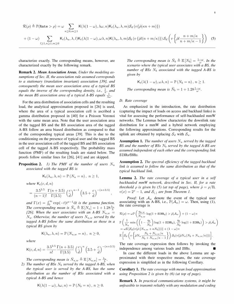
about 15% area is LOS in a ball of radius 150m around a userin these regions. The downlink rate distribution (both uplinkand downlink) obtained from simulations (as per Sec. II-E)and analysis (Lemma 2) is shown in Fig. 6 for the two citieswith two different different BS densities. The parameters (C,D) used in analysis for the specific geography are obtainedusing Fig. 5 and are given in Table II. The closeness of theanalytical results to those of the simulations validates (a) theability of the proposed simple blockage model to capture theblockage characteristics of dense urban settings, and (b) theload characterization for irregular association cells (Fig. 3) in ammW network. The closeness of the match builds confidencein the model and the derived design insights.

In the above plots any (C, D) pair from Fig. 5 can be used.However, it is observed that the match is better for the (C,D) pair with larger D (200-250m). This is due to the factthat the LOS fractional area (C2, say) beyond distance D isignored, which is a better approximation for larger D. It isstraightforward to allow LOS area outside D in the analysis(as shown in Appendix A) but estimating the same usingactual building locations is quite computationally intensive andtricky, as averaging needs to be done over a considerably largerarea. The fit procedure is simplified, though not sacrificing theaccuracy of the fit much (as seen), by setting C2 = 0 in themodel.

10

106

107

108

109

0

0.1

0.2

0.3

0.4

0.5

0.6

0.7

0.8

0.9

1

Rate threshold (bps)

Ra

te C

ove

rag

e

Simulation-actual building locationsAnalysis

Uplink

Downlink

(a) Manhattan

107

108

109

0

0.1

0.2

0.3

0.4

0.5

0.6

0.7

0.8

0.9

1

Rate threshold (bps)

Ra

te C

ove

rag

e

Simulation-actual building locations

Analysis

Uplink

Downlink

(b) Chicago

Fig. 6: Downlink rate distribution comparison from simulation and analysis for BS density 30 per sq. km in Manhattan (a) and 60 per sq.km in Chicago (b).

50 100 150 200 2500.2

0.3

0.4

0.5

0.6

0.7

0.8

0.9

1

Density (BS per sq. km)

Do

wn

link c

ove

rag

e

SNR - Analysis

SINR - Simulations

τ = -5, 0, 5, 10 dB

(a) Downlink

50 100 150 200 2500

0.1

0.2

0.3

0.4

0.5

0.6

0.7

0.8

0.9

1

Density (BS per sq. km)

Up

link c

ove

rag

e

SNR - Analysis

SINR - Simulations

τ = -5, 0, 5, 10 dB

(b)

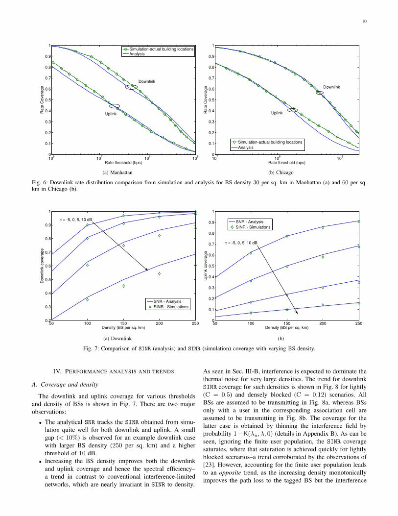
Fig. 7: Comparison of SINR (analysis) and SINR (simulation) coverage with varying BS density.

IV. PERFORMANCE ANALYSIS AND TRENDS

A. Coverage and density

The downlink and uplink coverage for various thresholdsand density of BSs is shown in Fig. 7. There are two majorobservations:

• The analytical SNR tracks the SINR obtained from simu-lation quite well for both downlink and uplink. A smallgap (< 10%) is observed for an example downlink casewith larger BS density (250 per sq. km) and a higherthreshold of 10 dB.

• Increasing the BS density improves both the downlinkand uplink coverage and hence the spectral efficiency–a trend in contrast to conventional interference-limitednetworks, which are nearly invariant in SINR to density.

As seen in Sec. III-B, interference is expected to dominate thethermal noise for very large densities. The trend for downlinkSINR coverage for such densities is shown in Fig. 8 for lightly(C = 0.5) and densely blocked (C = 0.12) scenarios. AllBSs are assumed to be transmitting in Fig. 8a, whereas BSsonly with a user in the corresponding association cell areassumed to be transmitting in Fig. 8b. The coverage for thelatter case is obtained by thinning the interference field byprobability 1−K(λu, λ, 0) (details in Appendix B). As can beseen, ignoring the finite user population, the SINR coveragesaturates, where that saturation is achieved quickly for lightlyblocked scenarios–a trend corroborated by the observations of[23]. However, accounting for the finite user population leadsto an opposite trend, as the increasing density monotonicallyimproves the path loss to the tagged BS but the interference

11

102

103

104

0.2

0.3

0.4

0.5

0.6

0.7

0.8

0.9

1

Density (BS per sq. km)

SIN

R C

ove

rag

e, P

(SIN

R>

τ)

C = 12 %

C = 50%

τ = 10, 5, 0 dB

(a) All BSs transmit

102

103

104

0.2

0.3

0.4

0.5

0.6

0.7

0.8

0.9

1

Density (BS per sq. km)

SIN

R C

ove

rag

e, P

(SIN

R>

τ)

C = 12%

C = 50%

τ = 10, 5, 0 dB

(b) BSs with an active user transmit

Fig. 8: SINR coverage variation with large densities for different blockage densities.

108

109

0

0.1

0.2

0.3

0.4

0.5

0.6

0.7

0.8

0.9

1

Rate threshold (bps)

Ra

te C

ove

rag

e

SimulationAnalysis

λ = 100, 150, 200 BS per sq. km.

(a) Downlink

106

107

108

0

0.1

0.2

0.3

0.4

0.5

0.6

0.7

0.8

0.9

1

Rate threshold (bps)

Ra

te C

ove

rag

e

SimulationAnalysis

λ = 50, 100, 200 BS per sq. km.

(b) Uplink

Fig. 9: Downlink and uplink rate coverage for different BS densities and fixed ω = 0.5.

is (implicitly) capped by the finite user density of 1000 persq. km.

B. Rate coverage

The variation of downlink and uplink rate distribution withthe density of infrastructure for a fixed A-BS fraction ω =0.5 is shown in Fig 9. Reducing the cell size by increasingdensity boosts the coverage and decreases the load per basestation. This dual benefit improves the overall rate drasticallywith density as shown in the plot. Further, the good matchof analytical curves to that of simulation also validates theanalysis for uplink and downlink rate coverage.

The variation in rate distribution with bandwidth is shownin Fig. 10 for a fixed BS density λ = 100 BS per sq. km andω = 1. Two observations can be made here: 1) median andpeak rate increase considerably with the availability of larger

bandwidth, whereas 2) cell edge rates exhibit a non-increasingtrend. The latter trend is due to the low SNR of the cell edgeusers, where the gain from bandwidth is counterbalanced bythe loss in SNR. Further, if the constraint of Rate = 0 forSNR < τ0 is imposed, cell edge rates would actually decreaseas shown in Fig. 10b due to the increase in P(SNR < τ0),highlighting the impossibility of increasing rates for power-limited users in mmW networks by just increasing the systembandwidth. In fact, it may be counterproductive.

C. Impact of co-existence

The rate distribution of a mmW only network and that ofa mmW-µW hybrid network is shown in Fig. 11 for differentmmW BS densities and fixed µW network density of µ = 5BS per sq. km. Offloading users from mmW to µW, whenthe link SNR drops below τmin = −10 dB improves the

12

106

107

108

109

0

0.1

0.2

0.3

0.4

0.5

0.6

0.7

0.8

0.9

1

Rate threshold (bps)

Ra

te C

ove

rag

e

B = 1 GHz

B = 2 GHz

B = 4 GHz

Uplink

Downlink

(a) τ0 = 0

106

107

108

109

0

0.1

0.2

0.3

0.4

0.5

0.6

0.7

0.8

0.9

1

Rate threshold (bps)

Ra

te C

ove

rag

e

B = 1 GHz

B = 2 GHz

B = 4 GHz

Uplink

Downlink

(b) τ0 = 0.1

Fig. 10: Effect of bandwidth and min SNR constraint (Rate = 0 for SNR < τ0) on rate distribution for BS density 100 per sq. km.

106

107

108

0

0.1

0.2

0.3

0.4

0.5

0.6

0.7

0.8

0.9

1

Rate threshold (bps)

Ra

te C

ove

rag

e

mmW only (τ0 = 0.1)

mmW only (τ0 = 0)

mmW+µWλ = 50, 80, 100 mmW BS per sq. km

Fig. 11: Downlink rate distribution for mmW only and hybrid networkfor different mmW BS density and fixed µW density of 5 BS per sq.km.

rate of edge users significantly, when the min SNR constraint(τ0 = −10 dB) is imposed. Such gain from co-existence,however, reduces with increasing mmW BS density, as thefraction of “poor” SNR users reduces. Without any such min-imum SNR consideration, i.e., τ0 = 0, mmW is preferred dueto the 100x larger bandwidth. So the key takeaway here is thatusers should be offloaded to a co-existing µW macrocellularnetwork only when reliable communication over the mmWlink is unfeasible.

D. Impact of self-backhauling

The variation of downlink rate distribution with the fractionof A-BSs ω in the network with BS density of 100 and 150 persq. km is shown in Fig. 12. As can be seen, providing wiredbackhaul to increasing fraction of BSs improves the overall

0 1 2 3 4 5 6 7 8 9 10

x 108

0

0.1

0.2

0.3

0.4

0.5

0.6

0.7

0.8

0.9

1

Rate threshold (bps)

Ra

te C

ove

rag

e

ω = 0.75

ω = 0.5

ω = 0.25

λ = 100 BS per sq.km

λ = 150 BS per sq.km

Fig. 12: Rate distribution with variation in ω

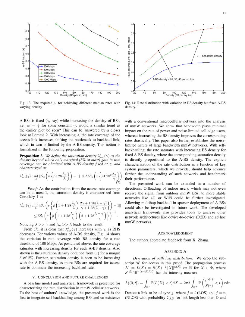
rate distribution. However “diminishing return” is seen withincreasing ω as the bottleneck shifts from the backhaul to theair interface rate. Further, it can be observed from the plot thatdifferent combinations of A-BS fraction and BS density, e.g.(ω = 0.25, λ = 150) and (ω = 0.5, λ = 100) lead to similarrate distribution. This is investigated further using Lemma 2in Fig. 13, which characterizes the different contours of (ω, λ)required to guarantee various median rates ρ50 (R(ρ50) = 0.5)in the network. For example, a median rate of 400 Mbps inthe network can be provided by either ω = 0.9, λ = 110 orω = 0.3, λ = 200. Thus, the key insight from these resultsis that it is feasible to provide the same QoS (median ratehere) in the network by either providing wired backhaul toa small fraction of BSs in a dense network, or by increasingthe corresponding fraction in a sparser network. In the aboveplots, the actual number of A-BSs in a given area increasedwith increasing density for a fixed ω, but if the density of

13

100 110 120 130 140 150 160 170 180 190 2000.1

0.2

0.3

0.4

0.5

0.6

0.7

0.8

0.9

1

Density (BS per sq. km)

A-B

S fra

ctio

n (

ω)

200 Mbps

400 Mbps

600 Mbps

800 Mbps

1000 Mbps

Fig. 13: The required ω for achieving different median rates withvarying density

A-BSs is fixed (γ, say) while increasing the density of BSs,i.e., ω = γ

λ for some constant γ, would a similar trend asthe earlier plot be seen? This can be answered by a closerlook at Lemma 2. With increasing λ, the rate coverage of theaccess link increases shifting the bottleneck to backhaul link,which in turn is limited by the A-BS density. This notion isformalized in the following proposition.

Proposition 3. We define the saturation density λδsat(γ) as thedensity beyond which only marginal (δ% at most) gain in ratecoverage can be obtained with A-BS density fixed at γ, andcharacterized as

λδsat(γ) : infλ‖Sd

(v

{ρ1.28

λuλ

})− 1‖ ≤ δ/Sb

(v

{ρ1.282 λu

γ

}).

(7)

Proof: As the contribution from the access rate coveragecan be at most 1, the saturation density is characterized fromCorollary 1 as

λδsat(γ) : infλ‖Sd

(v

{ρ

(1 + 1.28

λuλ

)2γ + 1.28(λ− γ)

γ + 1.28(λ− γ)

})− 1‖

≤ δSb(v

{ρ

(1 + 1.28

λuλ

)(2 + 1.28

λ− γγ

)})−1

.

Noticing λ >> γ and λu >> λ leads to the result.From (7), it is clear that λδsat(γ) increases with γ, as RHS

decreases. For various values of A-BS density, Fig. 14 showsthe variation in rate coverage with BS density for a ratethreshold of 100 Mbps. As postulated above, the rate coveragesaturates with increasing density for each A-BS density. Alsoshown is the saturation density obtained from (7) for a marginδ of 2%. Further, saturation density is seen to be increasingwith the A-BS density, as more BSs are required for accessrate to dominate the increasing backhaul rate.

V. CONCLUSION AND FUTURE CHALLENGES

A baseline model and analytical framework is presented forcharacterizing the rate distribution in mmW cellular networks.To the best of authors’ knowledge, the presented work is thefirst to integrate self-backhauling among BSs and co-existence

20 40 60 80 100 120 140 160 180 2000.1

0.2

0.3

0.4

0.5

0.6

0.7

0.8

Density (BS per sq. km)

Ra

te c

ove

rag

e, P

r(R

ate

> 1

00

Mb

ps

A-BS density = 20, 30, 40 per sq. km

Saturation density

Fig. 14: Rate distribution with variation in BS density but fixed A-BSdensity.

with a conventional macrocellular network into the analysisof mmW networks. We show that bandwidth plays minimalimpact on the rate of power and noise-limited cell edge users,whereas increasing the BS density improves the correspondingrates drastically. This paper also further establishes the noise-limited nature of large bandwidth mmW networks. With self-backhauling, the rate saturates with increasing BS density forfixed A-BS density, where the corresponding saturation densityis directly proportional to the A-BS density. The explicitcharacterization of the rate distribution as a function of keysystem parameters, which we provide, should help advancefurther the understanding of such networks and benchmarktheir performance.

The presented work can be extended in a number ofdirections. Offloading of indoor users, which may not evenreceive the signal from outdoor mmW BSs, to more stablenetworks like 4G or WiFi could be further investigated.Allowing multihop backhaul in sparser deployment of A-BSscould also be investigated in future work. The developedanalytical framework also provides tools to analyze othernetwork architectures like device-to-device (D2D) and ad hocmmW networks.

ACKNOWLEDGMENT

The authors appreciate feedback from X. Zhang.

APPENDIX A

Derivation of path loss distribution: We drop the sub-script ‘a’ for access in this proof. The propagation processN := L(X) = S(X)−1‖X‖α(X) on R for X ∈ Φ, whereS , 10−(χ+β)/10, has the intensity measure

Λ((0, t]) =

∫R2

P(L(X) < t)dX = 2πλ

∫R+

P(rα(r)

S(r)< t

)rdr.

Denote a link to be of type j, where j = l (LOS) and j = n(NLOS) with probability Cj,D for link length less than D and

14

Cj,D otherwise. Note by construction Cl,D + Cn,D = 1 andCl,D + Cn,D = 1. The intensity measure is then

Λ((0, t]) = 2πλ∑

j∈{l,n}

Cj,D

∫R+

P(rαj

Sj< t

)1(r < D)rdr

+ Cj,D

∫R+

P(rαj

Sj< t

)1(r > D)rdr

= 2πλE

[ ∑j∈{l,n}

(Cj,D − Cj,D)D2

21(Sj > Dαj/t)

+ Cj,D(tSj)

2/αj

21(Sj < Dαj/t) + Cj,D

(tSj)2/αj

21(Sj > Dαj/t)

]= λπ

∑j∈{l,n}

(Cj,D − Cj,D)D2FSj (Dαj/t)

+ t2/αj(

Cj,DζSj ,2/αj (Dαj/t) + Cj,DζSj ,2/αj

(Dαj/t)),

where FS denotes the CCDF of S, and ζS,n(x), ζS,n

(x)

denote the truncated nth moment of S given by ζS,n(x) ,∫ x0snfS(s)ds and ζ

S,n(x) ,

∫∞xsnfS(s)ds. Since S is

a Lognormal random variable ∼ lnN (m,σ2), where m =−0.1β ln 10 and σ = 0.1ξ ln 10. The intensity measure inLemma 1 is then obtained by using

FS(x) = Q

(lnx−m

σ

),

ζS,n(x) = exp(σ2n2/2 +mn)Q

(σ2n− lnx+m

σ

)ζS,n

(x) = exp(σ2n2/2 +mn)Q

(−σ

2n− lnx+m

σ

).

Now, since N is a PPP, the distribution of path loss to thetagged BS is then P(infX∈Φ L(X) > t) = Λ((0, t]).

APPENDIX BSINR distribution: Having derived the intensity measure

of N in Lemma 1, the distribution of SINR can be character-ized on the same lines as [36]. The key steps are highlightedbelow for completeness.

P(SINR > τ) = P

(PbGmaxL(X∗)−1∑

X∈Φ\{X∗} PbψXL(X)−1 + σ2N

> τ

)

= P(J +

σ2NL(X∗)

PbGmax<

1

τ

)=

∫l>0

P(J +

σ2N l

PbGmax<

1

τ|L(X∗) = l

)fL(X∗)(l)dl

where J = L(X∗)Gmax

∑X∈Φ\{X∗} ψXL(X)−1 and the distribu-

tion of L(X∗) is derived as

fL(X∗)(l) = − d

dlP(L(X∗) > l) = λ exp(−λM(l))M

′(l).

(8)The conditional CDF required for the above computation isderived from the the conditional Laplace transform givenbelow using the Euler’s characterization [37]

LJ,l(z) = E [exp(−zJ)|L(X∗) = l)]

= exp

(−Eψ

[∫u>l

(1− exp(−zlψ/u))Λ(du)

]),

where Λ(du) is given by (4).The inverse Laplace transform calculation required in the

above derivation could get computationally intensive in cer-tain cases and may render the analysis intractable. However,introducing Rayleigh small scale fading H ∼ exp(1), on eachlink improves the tractability of the analysis as shown below.Coverage with fading is

P

(PbGmaxHX∗L(X∗)−1∑

X∈Φ\{X∗} PbψXHXL(X)−1 + σ2N

> τ

)

=E

exp

− τσ2N

PbGmaxL(X∗)− τLX∗

∑X∈Φ\{X∗}

ψX

GmaxHXL(X)−1

(a)=

∫l>0

exp

(−

τσ2N

PbGmaxl − λEz

[∫u>l

M′(u)du

u(zl)−1 + 1

])fLX∗ (l)dl

(b)=λ

∫l>0

exp

(−

τσ2N

PbGmaxl − λM(l)Eψ

[1

1 + z

])

× exp

(−λEψ

[∫ zz+1

0M

{zl

(1

u− 1

)}du

])M′(l)dl

where z = τψGmax

, (a) follows using the Laplace functional ofpoint process N , (b) follows using integration by parts alongwith (8).

The above derivation assumed all BSs to be transmitting, butsince user population is finite, certain BSs may not have a userto serve with probability 1−K(λu, λ, 0). This is incorporatedin the analysis by modifying λ → λ(1 − K(λu, λ, 0)) in (a)above.

REFERENCES

[1] FCC, “National broadband plan recommmendations.” Available at: http://www.broadband.gov/plan/5-spectrum/r5.

[2] Cisco, “Cisco visual networking index: Global mobile data traffic fore-cast update, 2012-2017.” Whitepaper, available at: http://goo.gl/xxLT.

[3] F. Boccardi, R. W. Heath, A. Lozano, T. L. Marzetta, and P. Popovski,“Five disruptive technology directions for 5G,” IEEE Commun. Mag.,vol. 52, pp. 74–80, Feb. 2014.

[4] T. Rappaport et al., “Millimeter wave mobile communications for 5Gcellular: It will work!,” IEEE Access, vol. 1, pp. 335–349, May 2013.

[5] J. G. Andrews et al., “What will 5G be?,” IEEE J. Sel. Areas Commun.,vol. PP, June 2014.

[6] T. Baykas et al., “IEEE 802.15.3c: The first IEEE wireless standard fordata rates over 1 Gb/s,” IEEE Commun. Mag., vol. 49, pp. 114–121,July 2011.

[7] R. C. Daniels, J. N. Murdock, T. S. Rappaport, and R. W. Heath, “60GHz wireless: Up close and personal,” IEEE Microw. Mag., vol. 11,pp. 44–50, Dec. 2010.

[8] Z. Pi and F. Khan, “An introduction to millimeter-wave mobile broad-band systems,” IEEE Commun. Mag., vol. 49, pp. 101–107, June 2011.

[9] W. Roh et al., “Millimeter-wave beamforming as an enabling technologyfor 5G cellular communications: Theoretical feasibility and prototyperesults,” IEEE Commun. Mag., vol. 52, pp. 106–113, Feb. 2014.

[10] T. Rappaport et al., “Broadband millimeter-wave propagation measure-ments and models using adaptive-beam antennas for outdoor urbancellular communications,” IEEE Trans. Antennas Propag., vol. 61,pp. 1850–1859, Apr. 2013.

[11] S. Rangan, T. Rappaport, and E. Erkip, “Millimeter-wave cellularwireless networks: Potentials and challenges,” Proceedings of the IEEE,vol. 102, pp. 366–385, Mar. 2014.

[12] M. R. Akdeniz et al., “Millimeter wave channel modeling and cellularcapacity evaluation,” IEEE J. Sel. Areas Commun., vol. PP, June 2014.

[13] S. Larew, T. Thomas, and A. Ghosh, “Air interface design and ray tracingstudy for 5G millimeter wave communications,” IEEE Globecom B4GWorkshop, pp. 117–122, Dec. 2013.

[14] A. Ghosh et al., “Millimeter wave enhanced local area systems: A highdata rate approach for future wireless networks,” IEEE J. Sel. AreasCommun., vol. PP, June 2014.

15

[15] M. Abouelseoud and G. Charlton, “System level performance ofmillimeter-wave access link for outdoor coverage,” in IEEE WCNC,pp. 4146–4151, Apr. 2013.

[16] S. Singh, R. Mudumbai, and U. Madhow, “Interference analysis forhighly directional 60 GHz mesh networks: The case for rethinkingmedium access control,” IEEE/ACM Trans. Netw., vol. 19, pp. 1513–1527, Oct. 2011.

[17] Interdigital, “Small cell millimeter wave mesh backhaul,” Feb. 2013.Whitepaper, available at: http://goo.gl/Dl2Z6V.

[18] R. Taori and A. Sridharan, “In-band, point to multi-point, mm-Wavebackhaul for 5G networks,” in IEEE Intl. Workshop on 5G Tech., ICC,June 2014.

[19] J. S. Kim, J. S. Shin, S.-M. Oh, A.-S. Park, and M. Y. Chung, “Systemcoverage and capacity analysis on millimeter-wave band for 5G mobilecommunication systems with massive antenna structure,” Intl. Journalof Antennas and Propagation, vol. 2014, July 2014.

[20] M. Coldrey, J.-E. Berg, L. Manholm, C. Larsson, and J. Hansryd, “Non-line-of-sight small cell backhauling using microwave technology,” IEEECommun. Mag., vol. 51, pp. 78–84, Sept. 2013.

[21] S. W. Peters, A. Y. Panah, K. T. Truong, and R. W. Heath, “Relayarchitectures for 3GPP LTE-advanced,” EURASIP Journal on WirelessCommunications and Networking, 2009.

[22] S. Akoum, O. El Ayach, and R. Heath, “Coverage and capacity inmmWave cellular systems,” in Asilomar Conference on Signals, Systemsand Computers (ASILOMAR), pp. 688–692, Nov. 2012.

[23] T. Bai and R. W. Heath, “Coverage and rate analysis for millimeter wavecellular networks,” IEEE Trans. Wireless Commun., 2014. Submitted,available at http://arxiv.org/abs/1402.6430.

[24] T. Bai and R. W. Heath, “Coverage analysis for millimeter wave cellularnetworks with blockage effects,” in IEEE Global Conf. on Signal andInfo. Processing (GlobalSIP), pp. 727–730, Dec. 2013.

[25] T. Bai, R. Vaze, and R. W. Heath, “Analysis of blockage effects on urbancellular networks,” IEEE Trans. Wireless Commun., 2014. To appear.Available at: http://arxiv.org/abs/1309.4141.

[26] S. Singh, H. S. Dhillon, and J. G. Andrews, “Offloading in heterogeneousnetworks: Modeling, analysis, and design insights,” IEEE Trans. WirelessCommun., vol. 12, pp. 2484–2497, May 2013.

[27] J. G. Andrews, S. Singh, Q. Ye, X. Lin, and H. S. Dhillon, “An overviewof load balancing in HetNets: Old myths and open problems,” IEEEWireless Commun. Mag., vol. 21, pp. 18–25, Apr. 2014.

[28] The City of New York, “New York building perimeter data.” Online,available at: http://tinyurl.com/khlo69r.

[29] The City of Chicago, “Chicago building perimeter data.” Online, avail-able at: http://tinyurl.com/mccksq4.

[30] A. Guo and M. Haenggi, “Asymptotic deployment gain: A simpleapproach to characterize the SINR distribution in general cellularnetworks,” IEEE Trans. Commun., 2014. Submitted, available at:http://arxiv.org/abs/1404.6556.

[31] S. Yi, Y. Pei, and S. Kalyanaraman, “On the capacity improvement ofad hoc wireless networks using directional antennas,” in Intl. Symp. onMobile Ad Hoc Networking and Computing, MobiHoc, pp. 108–116,2003.

[32] H. Wang and M. Reed, “Tractable model for heterogeneous cellularnetworks with directional antennas,” in Australian CommunicationsTheory Workshop (AusCTW), pp. 61–65, Jan. 2012.

[33] J. Wildman, P. H. J. Nardelli, M. Latva-aho, and S. Weber, “On the jointimpact of beamwidth and orientation error on throughput in wirelessdirectional Poisson networks,” IEEE Trans. Wireless Commun., 2014.To appear, available at: http://arxiv.org/abs/1312.6057.

[34] F. Baccelli and B. Blaszczyszyn, Stochastic Geometry and WirelessNetworks, Volume I – Theory. NOW: Foundations and Trends inNetworking, 2009.

[35] Q. C. Li, H. Niu, G. Wu, and R. Q. Hu, “Anchor-booster basedheterogeneous networks with mmWave capable booster cells,” IEEEGlobecom B4G Workshop, Dec 2013.

[36] B. Blaszczyszyn, M. K. Karray, and H.-P. Keeler, “Using Poissonprocesses to model lattice cellular networks,” in Proc. IEEE Intl. Conf.on Comp. Comm. (INFOCOM), pp. 773–781, Apr. 2013.

[37] J. Abate and W. Whitt, “Numerical inversion of Laplace transforms ofprobability distributions,” ORSA Journal on Computing, vol. 7, no. 1,pp. 36–43, 1995.

[38] S. Singh, “Matlab code for numerical computation of total powerto noise ratio in mmW networks.” [Online]. Available : http://goo.gl/MF9qfd.

[39] S. Singh, F. Baccelli, and J. G. Andrews, “On association cells in randomheterogeneous networks,” IEEE Wireless Commun. Lett., vol. 3, pp. 70–73, Feb. 2014.

[40] J.-S. Ferenc and Z. Neda, “On the size distribution of Poisson Voronoicells,” Physica A: Statistical Mechanics and its Applications, vol. 385,pp. 518 – 526, Nov. 2007.

[41] S. M. Yu and S.-L. Kim, “Downlink capacity and base station density incellular networks,” in Intl. Symp. on Modeling Optimization in MobileAd Hoc Wireless Networks (WiOpt), pp. 119–124, May 2013.

[42] J. G. Andrews, F. Baccelli, and R. K. Ganti, “A tractable approach tocoverage and rate in cellular networks,” IEEE Trans. Commun., vol. 59,pp. 3122–3134, Nov. 2011.