Robust Inventory Management Using Tractable Replenishment Policies

Chuen-Teck See∗ Melvyn Sim†

April 2007

Abstract

We propose tractable replenishment policies for a multi-period, single product inventory control

problem under ambiguous demands, that is, only limited information of the demand distributions such

as mean, support and deviation measures are available. We obtain the parameters of the tractable

replenishment policies by solving a deterministic optimization problem in the form of second order

cone optimization problem (SOCP). Our framework extends to correlated demands and is developed

around a factor-based model, which has the ability to incorporate business factors as well as time

series forecast effects of trend, seasonality and cyclic variations. Computational results show that

with correlated demands, our model outperforms a state independent base-stock policy derived from

dynamic programming and an adaptive myopic policy.

∗Department of Industrial and Systems Engineering, National University of Singapore. Email:

see chuenteck@yahoo.com.sg†NUS Business School, National University of Singapore and Singapore MIT Alliance (SMA). Email: dsc-

simm@nus.edu.sg. The research of the author is supported by SMA, NUS Risk Management Institute and NUS academic

research grants R-314-000-066-122 and R-314-000-068-122.

1

1 Introduction

Inventory ties up working capital and incurs holding costs, reducing profit every day excess stock is

held. Good inventory management has hence become crucial to businesses as they seek to continually

improve their customer service and profit margins, in the heat of global competition and demand

variability. Baldenius and Reichelstein [3] offered perhaps the most convincing study of the contribution

of good inventory management to profitability. They studied inventories of publicly traded American

manufacturing companies between 1981 and 2000, and they concluded that “Firms with abnormally

high inventories have abnormally poor long-term stock returns. Firms with slightly lower than average

inventories have good stock returns, but firms with the lowest inventories have only ordinary returns”.

The ability to incorporate more realistic assumptions about product demand into inventory models is

one key factor to profitability. Practical models of inventory would need to address the issue of demand

forecasting while staying sufficiently immunized against uncertainty and maintaining tractability. In

most industrial contexts, demand is uncertain and hard to forecast. Many demand histories have

factors that behave like random walks that evolve over time with frequent changes in their directions

and rates of growth or decline. In practice, for such demand processes, inventory managers often rely

on forecasts based on a time series of prior demand, which are often correlated over time. For example,

demand may depend on factors such as market outlook, oil prices and so forth, and contains effects of

trend, seasonality, cyclic variation and randomness.

In this paper, we address the problem of optimizing multi-period inventory using factor-based de-

mand models, where the coefficients of the factors can be forecasted statistically, perhaps using historical

time-series data. We assume that the demands may be correlated and are ambiguous, that is, limited

information of the demand distributions (only the mean, support and deviation measures) are available.

Using robust optimization techniques, we developed a tractable methodology that uses past demand

realizations to adaptively control multi-period inventory. Our model also includes a range of features

such as delivery delay and capacity limit on order quantity.

Our work is closely related to the multi-period newsvendor problem, a well studied problem in oper-

ations research. For the single product newsvendor, it is well-known that the base-stock policy based on

a critical fractile is optimal. See Scarf [36, 37] and Zipkin [40]. Azoury [2] and Miller [32] later extended

the results to other classes of distribution. For correlated demands, Veinott [39], characterized condi-

tions under which a myopic policy is optimal. Extending the results of Veinott, Johnson and Thompson

[28] considered an autoregressive, moving-average (ARMA) demand process, zero replenishment lead-

2

time and no backlogs, and showed the optimality of a myopic policy when there demand in each period

is bounded. Lovejoy [30] showed that a myopic critical-fractile policy is optimal or near optimal in

some inventory models with parameter adaptive demand processes, citing exponential smoothing on

the demand process and bayesian updating on uniformly distributed demand as examples. Song and

Zipkin [38] addressed the case of Poisson demand, where the transition rate between states is governed

by a Markov process.

Sampling-based approximation have also been applied to the newsvendor problem. The key idea

is to represent uncertainty by a finite sample of scenarios and solve the sample average approximation

counterpart of the problem. While there is no requirement to know the full demand distribution, it is

assumed that N independent samples of the demand drawn from the true distribution are available.

The key to the quality of the solution is the number of samples. Levi, Roundy, and Shmoys [31] gave

theoretical results on the sample size required to achieve ε-optimal solution. They showed that when the

sample size is greater than 92ε2

(min(b,h)

b+h

)−2ln(2

δ ), the solution of the sample average approximation is at

most 1+ε times the optimal solution with probability of at least 1−δ, with b being the backlog cost and

h being the holding cost. Other sampling-based approaches include infinitesimal perturbation analysis

(see Glasserman et. al. [25]) which uses stochastic gradient estimation technique, and the concave

adaptive value estimation procedure, which successively approximates the objective cost function with

a sequence of piecewise linear functions (see Godfrey et. al., [26] and Powell et. al. [34]).

When only partial information on the underlying demand distribution is known, the problem is

commonly known as the distribution-free newsvendor model. Research on distribution-free inventory

control dates back to Scarf [35], where he considered a single period newsvendor problem and determined

the orders that minimize the maximum expected cost over all possible demand distributions with the

same first and second moments. Subsequent work on distribution-free newsvendor problem includes

Gallego and Moon [23], and Gallego, Ryan and Simchi-Levi [24], where they showed that a base-stock

policy is optimal for the multi-period newsvendor problem with discrete demand distributions.

More recently, Bertsimas and Thiele [13], Ben-Tal et.al. [4], and Beinstock and Ozbay [15] developed

new approaches to the distribution-free inventory control problem, which has the advantage of being

more tractable than sampling-based approaches. They employed robust optimization techniques to

guarantee the feasibility of the obtained solution for all possible values of the uncertain parameters

in the designated uncertainty set. The main idea in robust optimization is to immunize uncertain

mathematical optimization against infeasibility while preserving the tractability of the model, see Ben-

Tal and Nemirovski [5, 6, 7], Bertsimas and Sim [11, 12], Bertsimas, et al. [10], El-Ghaoui and Lebret

3

[20], and El-Ghaoui, et al. [21]. Our proposed model is related to this track of research, which has been

gaining substantial popularity as a useful methodology for handling uncertainty.

The paper is organized as follows. In Section 2 we describe a stochastic inventory model. We

formulate our robust inventory models in Section 3 and discuss extensions in Section 4. We describe

computational results in Section 5 and conclude the paper in Section 6.

Notations: Throughout this paper, we denote a random variable with the tilde sign such as y and

vectors with bold face lower case letters such as y. We use y′ to denote the transpose of vector y. Also,

denote y+ = max(y, 0), y− = max(−y, 0), and ‖y‖2 =√∑

y2i .

2 Stochastic Inventory Model

The stochastic inventory model involves the derivation of replenishment decisions over a discrete plan-

ning horizon consisting of a finite number of periods under stochastic demand. The demand for each

period is usually a sequence of random variables which are not necessarily identically distributed and

not necessarily independent. We consider an inventory system with T planning horizons from t = 1 to

t = T . External demands arrive at the inventory system and the system replenishes its inventory from

some central warehouse (or supplier) with ample supply. The time line of events is as follows:

1. At the beginning of the tth time period, before observing the demand, the inventory manager

places an order of xt at unit cost ct for the product to be arrived after a (fixed) order lead-time

of L periods. Orders placed at the beginning of the tth time period will arrive at the beginning of

t + Lth period. We assume that replenishment ceases at the end of the planning horizon, so that

the last order is placed in period T −L. Without loss of generality, we assume that purchase costs

for inventory are charged at the time of order. The case where purchase costs are charged at the

time of delivery can be represented by a straight-forward shift of cost indices.

2. At the beginning of each time period t, the inventory manager faces an initial inventory position

yt and receives an order of xt−L. The demand of inventory for the period is realized at the end of

the time period. After receiving a demand of dt, the inventory position at the end of the period

is yt + xt−L − dt.

3. Excess inventory is carried to the next period incurring a per-unit overage (holding) cost. On the

other hand, each unit of unsatisfied demand is backlogged (carried over) to the next period with

4

a per-unit underage (backlogging) penalty cost. At the last period, t = T , the cost penalty for

unmet demand can be accounted through the underage penalty cost.

We assume a risk neutral inventory manager whose objective is to determine the dynamic ordering

quantities xt from period t = 1 to period t = T − L so as to minimize the total expected ordering,

inventory overage (holding) and underage (backlog) costs in response to the uncertain demands. Observe

that for L ≥ 1, the quantities xt−L, t = 1, . . . , L are known values. They denote orders made before

period t = 1 and are inventories in the delivery pipeline when the planning horizon starts.

We introduce the following notations.

• dt: stochastic exogenous demand at period t

• dt: a vector of random demands from period 1 to t, that is, dt = (d1, . . . , dt)

• xt(dt−1): order placed at the beginning of the tth time period after observing dt−1. The first

period inventory order is denoted by x1(d0) = x01

• yt(dt−1): inventory position at the beginning of the tth time period

• ht: unit inventory overage (holding) cost charged on excess inventory at the end of the tth time

period

• bt: unit underage (backlog) cost charged on backlogged inventory at the end of the tth time period

• ct: unit purchase cost of inventory for orders placed at the tth time period

• St: the maximum amount that can be ordered at the tth time period.

We use xt(dt−1) to represent the non-anticipative replenishment policy at the beginning of period t.

That is, the replenishment decision is based solely on the observed information available at the beginning

of period t, which is the demand vector dt−1 = (d1, . . . , dt−1). Given the order quantity xt−L(dt−L−1)

and stochastic exogenous demand dt, the inventory position at the end of the t time period (which is

also the inventory position at start of t + 1 time period) is given by

yt+1(dt) = yt(dt−1) + xt−L(dt−L−1)− dt, t = 1, . . . , T. (1)

In resolving the initial boundary conditions, we adopt the following notations:

• The initial inventory position of the system is y1(d0) = y01.

5

• When L ≥ 1, the orders that are placed before the planning horizon starts are denoted by

xt(dt−1) = x0t , t = 1− L, . . . , 0.

Note that Equation (1) can be written using the cumulative demand up to period t and cumulative

order received as follows,

yt+1(dt) = y01︸︷︷︸

initial inventory

+min{L,t}∑

τ=1

x0τ−L

︸ ︷︷ ︸committed orders

+t∑

τ=L+1

xτ−L(dτ−L−1)

︸ ︷︷ ︸order decisions

−t∑

τ=1

dτ .

︸ ︷︷ ︸cumulative demands

(2)

Observe that positive (respectively negative) value of yt+1(dt) represents the total amount of inven-

tory overage (respectively underage) at the end of the period t after meeting demand. Thus, the total

expected cost, including ordering, inventory overage and underage charges is equal to

T∑

t=1

(E

(ctxt(dt−1)

)+ E

(ht(yt+1(dt))+

)+ E

(bt(yt+1(dt))−

)).

Therefore, the multi-period inventory problem can be formulated as a T stage stochastic optimization

model as follows,

ZSTOC = minT∑

t=1

(E

(ctxt(dt−1)

)+ E

(ht(yt+1(dt))+

)+ E

(bt(yt+1(dt))−

)).

s.t. yt+1(dt) = yt(dt−1) + xt−L(dt−L−1)− dt t = 1, . . . , T

0 ≤ xt(dt−1) ≤ St t = 1, . . . , T − L

(3)

The aim of the stochastic optimization model is to derive a feasible replenishment policy that

minimizes the expected ordering and inventory costs. That is, we seek a sequence of action rules that

advises the inventory manager the action to take in time t as a function of the current inventory level

and historical demand realizations. Unfortunately, the decision variables in Problem (3), xt(dt−1), t =

1 . . . T − L and yt(dt−1), t = 2 . . . T + 1 are functionals, which means Problem (3) is an optimization

problem with infinite number of variables and constraints, and hence generally intractable.

The stochastic optimization problem (3) can also be formulated as a dynamic programming problem.

For simplicity, assuming zero lead-time and no ordering capacity limit, the dynamic programming

requires the following updates on the value function:

Jt(yt, d1, . . . , dt−1) = minx≥0

E(ctx + rt(yt + x− dt)+

Jt+1(yt + x− dt, d1, . . . , dt−1, dt) | d1 = d1, . . . , dt−1 = dt−1

),

6

where rt(u) = ht max(u, 0) + bt max(−u, 0). Maintaining the value function Jt(·) is computationally

prohibitive, and hence most inventory control literatures identify conditions such that the value functions

are not dependent on past demand history, so that the state space is computationally amenable. For

instance, it is well known that when the lead-time is zero and the demands are independently distributed

across time periods, there exists base-stock levels, qt such that the following replenishment policy

xt(dt−1) = (qt − yt)+

is optimal. Note that in order to obtain an optimal state independent base-stock policy for positive

lead-time, L > 0, we require some restrictions on the cost parameters. See for instance, Zipkin [40].

3 Robust Inventory Model

One of the central problems in stochastic models with unknown distribution is how to properly account

for data uncertainty while maintaining tractability. Following the recent development of robust opti-

mization such as Chen, Sim and Sun [17], Chen, Sim, Sun and Zhang [18] and Chen and Sim [19], we

relax the assumption of full distributional knowledge and modify the representation of data uncertain-

ties with the aim of producing a computationally tractable model. We adopt the factor-based demand

model in which the demands are affinely dependent on some random primitive factors.

Factor-based Demand Model

We introduce a factor-based demand model in which the uncertain demand are affinely dependent on

zero mean random factors z ∈ <N as follows:

dt(z) ∆= dt = d0t +

N∑

k=1

dkt zk, t = 1, . . . , T,

where

dkt = 0 ∀k ≥ Nt+1,

and 1 ≤ N1 ≤ N2 ≤ . . . ≤ NT = N . Under a factor-based demand model, the random factors, zk,

k = 1, . . . , N are realized sequentially. At period t, the factors, zk, k = 1, . . . , Nt has already been

unfolded. In progressing to period t + 1, the new factors zk, k = Nt + 1, . . . , Nt+1 are made available.

Demand that is affected by random noise or shocks can be represented by the factor-based demand

model. For independently distributed demand, which is assumed in most inventory models, we have

dt(z) = d0t + zt, t = 1, . . . , T,

7

in which zt are independently distributed. However, in many industrial contexts, demands across

periods may be correlated. In fact, many demand histories behave more like random walks over time

with frequent changes in directions and rate of growth or decline. See Johnson and Thompson [28] and

Graves [27]. In those settings, we may consider standard forecasting techniques such as an ARMA(p, q)

demand process (see Box et al. [16]) as follows

dt(z) =

d0t if t ≤ 0p∑

j=1

φidt−i(z) + zt +min{q,t−1}∑

j=1

θizt−j otherwise

for some constants coefficients φ1, . . . , φp, θ1, . . . , θq. Indeed, its is easy to show by induction that dt(z)

can be expressed in the form of a factor-based demand model. Song and Zipkin [38] presented a

world driven demand model where the demand is Poisson with rate controlled by finite Markov states

representing different business environment. Unfortunately, it is difficult to determine exhaustively the

business states and its state transition probabilities. On the other hand, factor-based models have been

used extensively in finance for modeling returns as affine functions of external factors, in which the

coefficients of the factors can be determined statistically. In the same way, we can apply the factor-

based demand model to characterize the influence of demands with external factors such as market

outlook, oil prices and so forth. Effects of trend, seasonality, cyclic variation, and randomness can also

be incorporated.

Instead of assuming full distributions on the factors, which is practically prohibitive, we adopt a

modest distributional assumption on the random factors, such as known means, supports and some

aspects of deviations. The factors may be partially characterized using the forward and backward

deviations, which are recently introduced by Chen, Sim and Sun [17].

Definition 1 Given a random variable z with zero mean, the forward deviation is defined as

σf (z) ∆= supθ>0

{√2 ln(E(exp(θz)))/θ2

}(4)

and backward deviation is defined as

σb(z) ∆= supθ>0

{√2 ln(E(exp(−θz)))/θ2

}. (5)

Given a sequence of independent samples, we can essentially estimate the magnitude of the deviation

measures from (4) and (5). Some of the properties of the deviation measures include:

8

Proposition 1 (Chen, Sim and Sun [17])

Let σ, p and q be respectively the standard, forward and backward deviations of a random variable, z

with zero mean.

(a) Then p ≥ σ and q ≥ σ. If z is normally distributed, then p = q = σ.

(b) For all θ ≥ 0,

P(z ≥ θp) ≤ exp(−θ2/2);

P(z ≤ −θq) ≤ exp(−θ2/2).

Proposition 1(a) shows that the forward and backward deviations are no less than the standard devia-

tion of the underlying distribution, and under normal distribution, these two values coincide with the

standard deviation. As exemplified in Proposition 1(b), the deviation measures provide an easy bound

on the distributional tails.

The forward and backward deviations can be bounded from the support of z as follows:

Theorem 1 (Chen, Sim and Sun [17]) If z has zero mean and distributed in [−z, z], z, z > 0, then

σf (z) ≤ σf (z) =z + z

2

√g

(z − z

z + z

)

and

σb(z) ≤ σb(z) =z + z

2

√g

(z − z

z + z

),

where

g(µ) = 2 maxs>0

{φµ(s)− µs

s2

},

and

φµ(s) = ln

(es + e−s

2+

es − e−s

2µ

).

Moreover, the bounds are tight.

Note that the forward and backward deviations may be infinite for heavier-tailed distributions. The

advantage of using the forward and backward deviations is the ability to capture distributional asym-

metry and stochastic independence, while keeping the resultant optimization model computationally

amicable. The interested reader may refer to Natarajan et al. [33] for the computational experience of

using the forward and backward deviations in minimizing the Value-at-Risk of a portfolio, which gives

surprisingly good out-of-sample performance on real-life data.

In this paper, we adopt the random factor model introduced by Chen and Sim [19], which encom-

passes most of the uncertainty models found in the literatures of robust optimization.

9

Assumption U: We assume that the random factors {zj}j=1:N are zero mean random variables, with

positive definite covariance matrix, Σ. Let W = {z : −z ≤ z ≤ z} denotes the smallest compact convex

set containing the support of z. We denote a subset, I ⊆ {1, . . . , N}, which can be an empty set, such

that zj , j ∈ I are stochastically independent. Moreover, the corresponding forward and backward

deviations (or their bounds used in Theorem 1) are given by pj = σf (zj) > 0 and qj = σb(zj) > 0

respectively for j ∈ I and that pj = qj = ∞ for j /∈ I.

Bound on E((·)+)

In the absence of full distribution, it would be meaningless to evaluate the optimal objective as depicted

in the stochastic optimization Problem (3). Instead, we aim to minimize a good upper bound on the

objective function. Such approach of soliciting inventory decisions based on partial demand information

is not new. In the 50s, Scarf [35] considered a min-max newsvendor problem with uncertain demand d

given by only its mean and standard deviations. Scarf was able to obtain solutions to the tight upper

bound of the newsvendor problem. The central idea in addressing such problem is to solicit a good

upper bound on E((·)+), which appears at the objective of the newsvendor problem and also in Problem

(3). The following result is well known.

Proposition 2 (Optimal upper bound, Lo [29] and Bertsimas and Popescu [14]) Let z be a

random variable in [−µ,∞) with mean µ and standard deviation σ, then for all a ≥ −µ,

E((z − a)+) ≤

12

(−a +

√σ2 + a2

)if a ≥ σ2−µ2

2µ

−aµ2

µ2 + σ2+ µ

σ2

µ2 + σ2if a < σ2−µ2

2µ

.

Moreover, the bound is tight.

Interestingly, Bertsimas and Thiele [13] used the bound of Proposition 2 to calibrate the “budget of

uncertainty” parameter (see Bertsimas and Sim [12]) in their robust inventory models. Unfortunately,

it is generally computationally intractable to evaluate tight probability bounds involving multivariate

random variables with known moments and support information (see Bertsimas and Popescus [14]). We

adopt the bounds of Chen and Sim [19] to evaluate the expected positive of an affine sum of random

variables under the Assumption U.

Definition 2 We say a function, f(z) is non-zero crossing with respect to z ∈ W if at least one of the

following conditions hold

10

1. f(z) ≥ 0 ∀z ∈ W

2. f(z) ≤ 0 ∀z ∈ W.

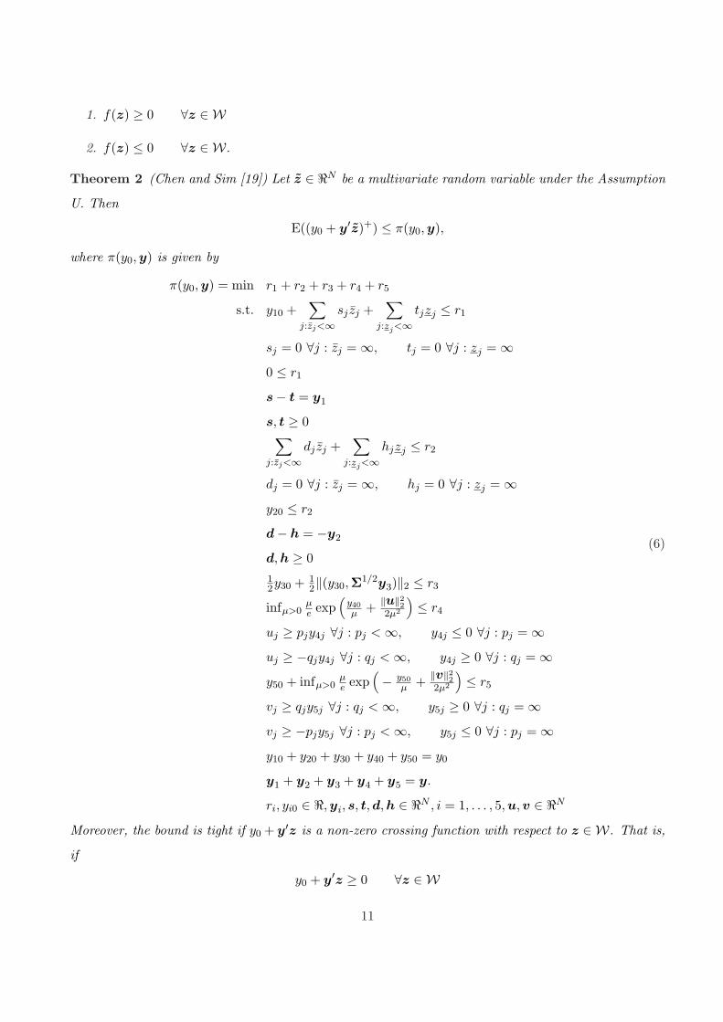
Theorem 2 (Chen and Sim [19]) Let z ∈ <N be a multivariate random variable under the Assumption

U. Then

E((y0 + y′z)+) ≤ π(y0, y),

where π(y0, y) is given by

π(y0, y) = min r1 + r2 + r3 + r4 + r5

s.t. y10 +∑

j:zj<∞sj zj +

∑

j:zj<∞tjzj ≤ r1

sj = 0 ∀j : zj = ∞, tj = 0 ∀j : zj = ∞0 ≤ r1

s− t = y1

s, t ≥ 0∑

j:zj<∞dj zj +

∑

j:zj<∞hjzj ≤ r2

dj = 0 ∀j : zj = ∞, hj = 0 ∀j : zj = ∞y20 ≤ r2

d− h = −y2

d, h ≥ 012y30 + 1

2‖(y30,Σ1/2y3)‖2 ≤ r3

infµ>0µe exp

(y40

µ + ‖u‖222µ2

)≤ r4

uj ≥ pjy4j ∀j : pj < ∞, y4j ≤ 0 ∀j : pj = ∞uj ≥ −qjy4j ∀j : qj < ∞, y4j ≥ 0 ∀j : qj = ∞y50 + infµ>0

µe exp

(− y50

µ + ‖v‖222µ2

)≤ r5

vj ≥ qjy5j ∀j : qj < ∞, y5j ≥ 0 ∀j : qj = ∞vj ≥ −pjy5j ∀j : pj < ∞, y5j ≤ 0 ∀j : pj = ∞y10 + y20 + y30 + y40 + y50 = y0

y1 + y2 + y3 + y4 + y5 = y.

ri, yi0 ∈ <,yi, s, t, d, h ∈ <N , i = 1, . . . , 5,u, v ∈ <N

(6)

Moreover, the bound is tight if y0 + y′z is a non-zero crossing function with respect to z ∈ W. That is,

if

y0 + y′z ≥ 0 ∀z ∈ W

11

we have E(( y0 + y′z )+

)= π(y0,y) = y0. Likewise, if

y0 + y′z ≤ 0 ∀z ∈ W,

we have E(( y0 + y′z )+

)= π(y0,y) = 0.

Remark 1: Due to the presence of the constraints, infµ>0 µ exp(

aµ + b2

µ2

)≤ c, the set of constraints

in Problem (6) is not exactly second order cone representable (see Ben-Tal and Nemirovski [8]). Fortu-

nately, using a few second order cones, we can accurately approximate such constraints to good a level

of numerical precision. The interested readers can refer to Chen and Sim [19].

Remark 2: Note that under the Assumption U, it is not necessary to provide all the information such

as forward and backward deviations and supports. So, whenever such information is unavailable, we

can assign an infinite value to the corresponding parameter. For instance, suppose the factor zj has

support in [−µ,∞), standard deviation, σ and unknown forward and backward deviations, we would

set zj = µ, zj = ∞, pj = qj = ∞. With more information on the factors, the bound of Problem (6) is

never worse off.

Remark 3: In the absence of uncertainty, the non-zero crossing condition ensures that the bound is

tight. That is, y+ = E(y+) = π(y,0).

We next show for a univariate random variable with one-sided support, the bound of Theorem 2 is

as tight as Proposition 2.

Proposition 3 Let z be a random variable in [−µ,∞) with mean µ and standard deviation σ, then for

all a ≥ −µ,

E((z − a)+) ≤ π(−a, 1) =

12

(−a +

√σ2 + a2

)if a ≥ σ2−µ2

2µ

−aµ2

µ2 + σ2+ µ

σ2

µ2 + σ2if a < σ2−µ2

2µ

Proof : See Appendix A.

We can further improve the bound if the distribution of the random variable z is sufficiently light

tailed such that the forward and backward deviations are close to its standard deviations, such as those

of normal and uniform distribution. Figure 1 compares the bounds of E((z − a)+) in which µ = 1 and

σ = σf (z) = σb(z) = 2. Bound 1 corresponds to the bound of Proposition 2, while Bound 2 corresponds

to the bound Theorem 2. Clearly, despite the lack of tightness results, incorporating the forward and

backward deviations can potentially improve the bound on E((z − a)+).

12

−1 0 1 2 3 4 5 6 7 8 90

0.1

0.2

0.3

0.4

0.5

0.6

0.7

0.8

0.9

1

a

Bound 1Bound 2

Figure 1: Comparing bounds of E((z − a)+)

3.1 Tractable Replenishment Policies

Having introduced the demand uncertainty model, a suitable approximation of the replenishment policy

xt(dt−1) is needed to obtain a tractable formulation. That is, we seek a formulation in which the policy

can be obtained by solving a optimization problem that runs in polynomial time and scalable across

time period. We review two tractable replenishment policies, static as well as linear with respect to

the random factors of demand, which have recently been proposed in robust optimization literatures.

We introduced a new replenishment policy, known as the truncated linear replenishment policy, which

improves over these policies.

Static replenishment policy

The static replenishment policy proposed by Bertsimas and Thiele [13], is a tractable one where the

order decisions are not influenced by the random factors of demand. A tractable model under such

replenishment policy is as follows:

ZSRP = minT∑

t=1

(ctx

0t + htπ

(y0

t+1, yt+1

)+ btπ

(−y0

t+1,−yt+1

))

s.t. y0t+1 = y0

t + x0t−L − d0

t t = 1, . . . , T

ykt+1 = yk

t − dkt k = 1, . . . , N, t = 1, . . . , T

0 ≤ x0t ≤ St t = 1, . . . , T − L,

(7)

13

with y01 being the initial inventory position and yk

1 = 0 for all k = 1, . . . , N . For L ≥ 1, x0t are the

known committed orders made at time periods t = 1− L, . . . , 0.

Theorem 3 The expected cost of the stochastic inventory problem under the static replenishment policy,

xSRPt (dt−1) = x0∗

t t = 1, . . . , T − L

in which x0∗t , t = 1, . . . , T − L are the optimal solution of Problem (7), is at most ZSRP .

Proof : See Appendix B.

Linear replenishment policy

A more refined replenishment policy introduced in Ben Tal et. al [4], and Chen, Sim and Sun [17] is

the linear replenishment policy where the order decisions are affinely dependent on the random factors

of demand. That is

xLRPt (dt−1) = x0

t + x′tz,

in which the vector xt = (x1t , . . . , x

Nt ) satisfies the following non-anticipative constraints,

xkt = 0 ∀k ≥ Nt.

Since the order decision is made at the beginning of the tth period, the non-anticipative constraints

ensure that the linear replenishment policy is not influenced by demand factors that are unavailable up

to the beginning of the tth period. The model for the linear replenishment policy is as follows:

ZLRP = minT∑

t=1

(ctx

0t + htπ

(y0

t+1, yt+1

)+ btπ

(−y0

t+1,−yt+1

))

s.t. ykt+1 = yk

t + xkt−L − dk

t k = 0, . . . , N, t = 1, . . . , T

xkt = 0 ∀k ≥ Nt, t = 1, . . . , T − L

0 ≤ x0t + x′tz ≤ St ∀z ∈ W t = 1, . . . , T − L,

(8)

with y01 being the initial inventory position and yk

1 = 0 for all k = 1, . . . , N . For L ≥ 1, x0t are the

known committed orders made at time periods t = 1− L, . . . , 0.

Note that under the box uncertainty set W, it is well known that the robust counterpart

0 ≤ x0t + x′tz ≤ St ∀z ∈ W

can be represented concisely as linear constraints. See for instance Ben-Tal et. al. [4] and Chen, Sim

and Sun [17]. Therefore, Problem (8) is essentially a second order cone optimization problem.

14

Theorem 4 The expected cost of the stochastic inventory problem under the linear replenishment policy,

xLRPt (dt−1) = x0∗

t + x∗t′z t = 1, . . . , T − L

in which xk∗t , k = 0, . . . , N, t = 1, . . . , T − L are the optimal solution of Problem (8), is at most ZLRP .

Moreover, ZLRP ≤ ZSRP .

Proof : See Appendix C.

Truncated linear decision policy

More recently, Chen, Sim, Sun and Zhang [18] developed a deflected linear decision rule that improves

upon linear decision rule in the approximation of multi-period stochastic optimization problems. Specific

to inventory control, we introduce the truncated linear replenishment policy as follows:

xTLRPt (dt−1) = min

{max

{x0

t + x′tz, 0}

, St

},

in which the vector xt = (x1t , . . . , x

Nt ) satisfies the following non-anticipative constraints,

xkt = 0 ∀k ≥ Nt.

Note that the truncated linear replenishment policy has an embedded linear replenishment policy and

that

0 ≤ xTLRPt (dt−1) ≤ St.

We first introduce the following result.

Theorem 5 Let z ∈ <N be a multivariate random variable under Assumption U. Then

E

(y0 + y′z +

p∑

i=1

(x0

i + xi′z

)+)+

≤ η((y0, y), (x0

1, x1), . . . , (x0p, xp)) (9)

where

η((y0, y), (x01, x1), . . . , (x0

p,xp))

= minw0

i ,wi,i=1,...,p

{π

(y0 +

p∑

i=1

w0i ,y +

p∑

i=1

wi

)+

p∑

i=1

(π(−w0

i ,−wi) + π(x0i − w0

i , xi −wi))}

.

Moreover, the bound is tight if y0 + y′z +∑p

i=1

(x0

i + xi′z

)+ and x0i + xi

′z, i = 1, . . . , p are non-zero

crossing functions with respect to z ∈ W.

15

Proof : See Appendix D.

Remark: In the absence of uncertainty, the non-zero crossing condition ensures that the bound is tight.

That is,

(y0 +

p∑

i=1

(x0

i

)+)+

= E

(y0 +

p∑

i=1

(x0

i

)+)+

= η((y0,0), (x0

1,0), . . . , (x0p,0)).

The model for the truncated linear replenishment policy is as follows:

ZTLRP = minT∑

t=1

ctπ(x0t , xt) +

L∑

t=1

(htπ(y0

t+1, yt+1) + btπ(−y0t+1,−yt+1)

)+

T∑

t=L+1

(htη

((y0

t+1, yt+1), (−x01,−x1), . . . , (−x0

t−L,−xt−L))

+

btη((−y0

t+1,−yt+1), (x01 − St,x1), . . . , (x0

t−L − St, xt−L)) )

s.t. ykt+1 = yk

t + xkt−L − dk

t k = 0, . . . , N, t = 1, . . . , T

xkt = 0 ∀k ≥ Nt, t = 1, . . . , T − L

(10)

with y01 being the initial inventory position and yk

1 = 0 for all k = 1, . . . , N . For L ≥ 1, x0t are the

known committed orders made at time periods t = 1− L, . . . , 0.

Theorem 6 The expected cost of the stochastic inventory problem under the truncated linear replen-

ishment policy,

xTLRPt (dt−1) = min

{max

{x0∗

t + x∗t′z, 0

}, St

}t = 1, . . . , T − L

in which xk∗t , k = 0, . . . , N , t = 1, . . . , T−L are the optimal solution of Problem (10), is at most ZTLRP .

Moreover, ZTLRP ≤ ZLDR.

Proof : See Appendix E.

Remark : For the case of unbounded ordering quantity, that is, St = ∞, the truncated linear replen-

ishment policy becomes,

xTLRPt (dt−1) = max

{x0

t + x′tz, 0}

,

16

and we can simplify Problem (10) as follows

ZTLRP = minT∑

t=1

ctπ(x0t ,xt) +

L∑

t=1

(htπ(y0

t+1, yt+1) + btπ(−y0t+1,−yt+1)

)+

T∑

t=L+1

(htη

((y0

t+1, yt+1), (−x01,−x1), . . . , (−x0

t−L,−xt−L))

+

btπ(−y0

t+1,−yt+1

) )

s.t. ykt+1 = yk

t + xkt−L − dk

t k = 0, . . . , N, t = 1, . . . , T

xkt = 0 ∀k ≥ Nt, t = 1, . . . , T − L.

(11)

Rolling horizon implementation

In practice, the replenishment policies may be implemented in a rolling horizon manner. That is, the

model is solved repeatedly with updated data. See Zipkin [40] and Ben-Tal et. al. [4]. In the rolling

horizon implementation, new order decisions are generated whenever demand realizations are observed.

The inventory manager re-solves in each period t Problem (10) for the remaining periods t, t + 1, . . . T ,

starting from initial inventory that are the actual ones, that is, those resulting from the earlier decisions

and the demand realized in periods 1, 2, . . . , t−1. The implementation requires only minor adjustments

to the model. The first run of any rolling horizon model is identical to the corresponding run of a fixed

horizon model. Then, to execute the second run we reduce the horizon by one period, set the order

decisions according to their optimal values in the first run, and fix the starting inventory according to

the realization of demand and replenishment decision from the previous period. Since more accurate

information are used each time the model is solved, the results will only improve.

4 Other extensions

In this section, we discuss some extension to the basic model.

4.1 Fixed ordering cost

Unfortunately, with fixed ordering cost, the inventory replenishment problem becomes nonconvex and

is much harder to address. Using the idea of Bertsimas and Thiele [13], we can formulate a restricted

problem where the time period in which the orders that can be placed is determined at the start of the

17

planning horizon as follows:

ZSTOCF = minT∑

t=1

(E

(ctxt(dt−1) + Ktrt + ht(yt+1(dt))+

)+ E

(bt(yt+1(dt))−

)).

s.t. yt+1(dt) = yt(dt−1) + xt−L(dt−L−1)− dt t = 1, . . . , T

0 ≤ xt(dt−1) ≤ Strt t = 1, . . . , T − L

rt ∈ {0, 1} t = 1, . . . , T − L.

(12)

In Problem (12), inventory can only be replenished at period where the corresponding binary variable

rt takes the value of one. We can then incorporate the tractable replenishment policies developed in

the previous section. The resulting optimization model is a conic integer program, which is already

addressed in commercial solvers such as CPLEX 10.1. Admittedly, algorithms for solving conic integer

program are still at their infancy. On the theoretical front, Atamturk and Narayanan [1] recently

described general-purpose conic mixed-integer rounding cuts based on polyhedral conic substructures

of second-order conic sets, which can be readily incorporated in branch-and-bound algorithms that

solve continuous conic programming relaxations at the nodes of the search tree. Their preliminary

computational experiments shows that the new cuts are quite effective in reducing the integrality gap

of continuous relaxations of conic mixed-integer programs.

4.2 Supply chain networks

The models we have presented in the preceding section can also be extended to more complex supply

chain networks such as the series system, or more generally the tree network. These are multi-stage

system where goods transit from one stage to the next stage, each time moving closer to their final

destination. In many supply chains, the main storage hubs, or the sources of the network, receive

their supplies from outside manufacturing plants in a tree-like hierarchical structure and send items

throughout the network until they finally reach the stores, or the sinks of the network. The extension

to tree structure uses the concept of echelon inventory and closely follows Bertsimas and Thiele [13].

We refer interested readers to their paper.

5 Computation Studies

In our computation studies, we compared the policy obtained from deterministic approximation of

robust optimization model to policies obtained from stochastic dynamic programming. We consider a

18

multi-period inventory control problem evaluated under the truncated linear decision policy framework.

The demand process we considered is motivated by Graves [27] as follows:

dt(z) = zt + αzt−1 + αzt−2 + . . . + αz1 + µ, (13)

where the mean µ = 100 and shocks factors zt being independently uniform distributed random variables

in [−20, 20], which has standard, forward and backward deviations of approximately 11.55. To reduce

the search effort needed for obtaining solutions from the dynamic programming algorithm, we have used

the uniform distributions which has bounded support. Observe that the demand process of Equation

(13) for t ≥ 2 can be expressed recursively as

dt(z) = dt−1(z)− (1− α)zt−1 + zt. (14)

Hence, this demand process is an integrated moving average (IMA) process of order (0, 1, 1). See also

Box et al. [16]. Note that given µ = dt−1(z)− (1− α)zt−1 at time period t, the distribution of dt(z) is

uniform in [−20 + µ, 20 + µ]. A range of demand process can be modeled by varying α. With α = 0,

the demand process follows an i.i.d process of uniformly distributed random variables in [80, 120]. As

α grows, the demand process becomes non-stationary and less stable with increasing variance. When

α = 1, the demand process is random walk on a continuous state space.

We consider problem with T = 5 so that the demand, dT (z) is nonnegative for all α ∈ [0, 1]. The

lead-time, L is zero, unit ordering cost ct = 2, and unit holding cost ht = 7 at all periods t = 1, . . . , T .

The backlog costs at periods t = 1, . . . , T − 1, are bt = 10. Since unfulfilled demands are lost at the end

of T , we set a relatively high backlog cost, bT = 500, to penalize unfulfilled demand at the last period.

The maximum order quantities, St, are set to 140 and we vary α from 0 to 1 in steps of 0.2.

We obtained the truncated linear replenishment policy (TLRP) by formulating Problem (10) using

an in-house developed software, PROF (Platform for Robust Optimization Formulation). The Matlab

based software is essentially a modeling platform for robust optimization that contains reusable functions

for modeling multi-period robust optimization using decision rules. After formulating the model, it

calls upon CPLEX 10.1 for solution. We have implemented bounds for π(·) of Equation (6) and η(·) of

Theorem 5. For T = 5, the size of the problem we consider is presented in Table 1. Our computation

was carried out on a 2.8GHz desktop with 2Mb memory. Computational time depends on the number

of period. For T = 5, it typically took less than 1 seconds to solve for the TLRP model. For T = 15, it

typically took about 4 seconds.

19

Number of affine constraints 5911

Number of free variables 3366

Number of non-negative variables 1700

Number of L2 cones 12

Number of L3 cones 1226

Number of L4 cones 38

Number of L5 cones 50

Number of L6 cones 72

Number of L7 cones 27

Table 1: Size of the TLRP model, where Ln = {(x0,x) ∈ < × <n−1 : ‖x‖2 ≤ x0}.

t zt dt xTRLPt yt+1

1 18.0 118.0 102.5 -15.5

2 19.3 126.5 136.3 -5.7

3 19.8 134.7 138.5 -1.9

4 -14.2 108.6 140.0 29.5

5 -2.0 115.2 105.2 19.5

Table 2: A sample path of the truncated linear replenishment policy.

The below example, solved for α = 0.4, serves as an illustration of the truncated linear replenishment

policy.

x01

x02

x03

x04

x05

=

102.5

103.0

101.4

107.5

105.6

x′1

x′2

x′3

x′4

x′5

=

0 0 0 0

1.85 0 0 0

0.24 1.70 0 0

0.19 0.18 1.42 0

0.32 0.32 0.38 1.40

In Table (2), we show a sample path of the truncated linear replenishment policy,

xTLRPi (z) = min{(x0

i + x′iz)+, 140}.

We benchmark our solutions against heuristics based on dynamic programming, where the optimal

20

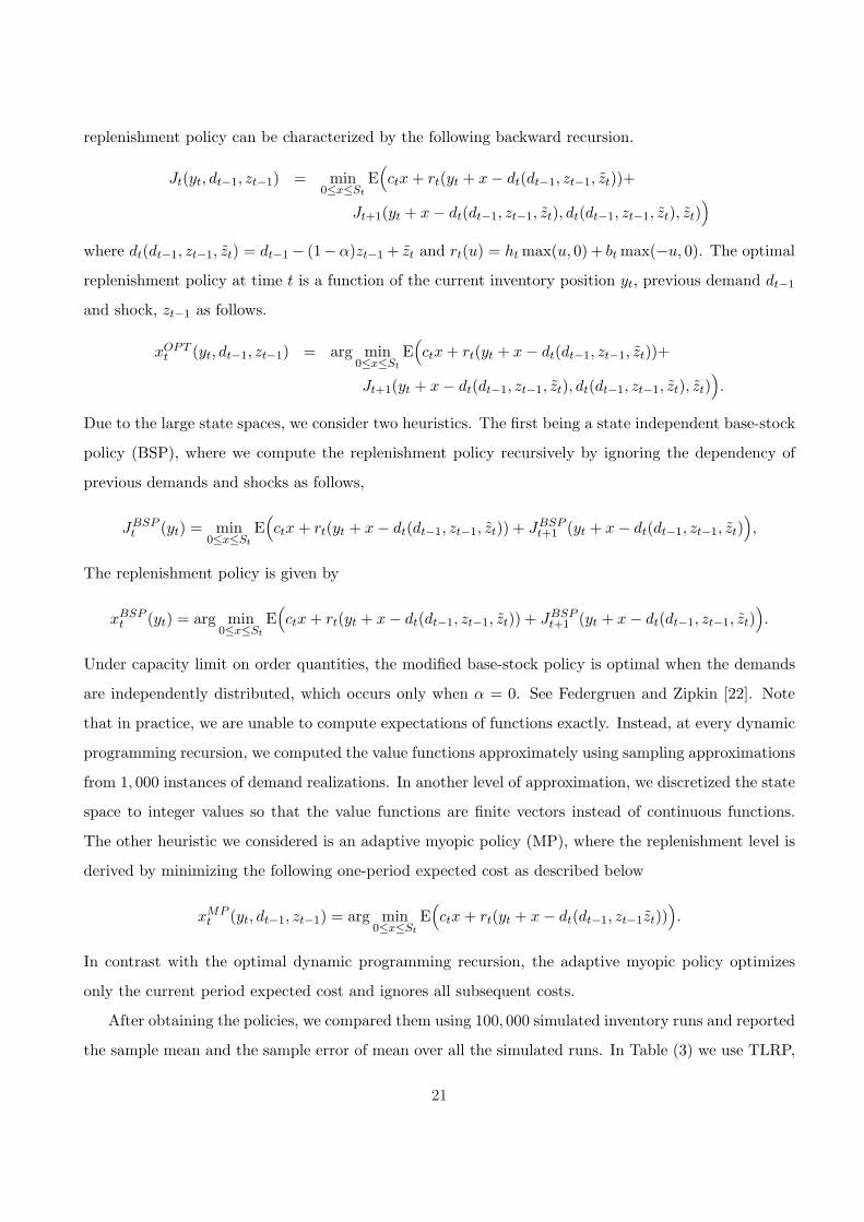
replenishment policy can be characterized by the following backward recursion.

Jt(yt, dt−1, zt−1) = min0≤x≤St

E(ctx + rt(yt + x− dt(dt−1, zt−1, zt))+

Jt+1(yt + x− dt(dt−1, zt−1, zt), dt(dt−1, zt−1, zt), zt))

where dt(dt−1, zt−1, zt) = dt−1− (1−α)zt−1 + zt and rt(u) = ht max(u, 0) + bt max(−u, 0). The optimal

replenishment policy at time t is a function of the current inventory position yt, previous demand dt−1

and shock, zt−1 as follows.

xOPTt (yt, dt−1, zt−1) = arg min

0≤x≤St

E(ctx + rt(yt + x− dt(dt−1, zt−1, zt))+

Jt+1(yt + x− dt(dt−1, zt−1, zt), dt(dt−1, zt−1, zt), zt)).

Due to the large state spaces, we consider two heuristics. The first being a state independent base-stock

policy (BSP), where we compute the replenishment policy recursively by ignoring the dependency of

previous demands and shocks as follows,

JBSPt (yt) = min

0≤x≤St

E(ctx + rt(yt + x− dt(dt−1, zt−1, zt)) + JBSP

t+1 (yt + x− dt(dt−1, zt−1, zt)),

The replenishment policy is given by

xBSPt (yt) = arg min

0≤x≤St

E(ctx + rt(yt + x− dt(dt−1, zt−1, zt)) + JBSP

t+1 (yt + x− dt(dt−1, zt−1, zt)).

Under capacity limit on order quantities, the modified base-stock policy is optimal when the demands

are independently distributed, which occurs only when α = 0. See Federgruen and Zipkin [22]. Note

that in practice, we are unable to compute expectations of functions exactly. Instead, at every dynamic

programming recursion, we computed the value functions approximately using sampling approximations

from 1, 000 instances of demand realizations. In another level of approximation, we discretized the state

space to integer values so that the value functions are finite vectors instead of continuous functions.

The other heuristic we considered is an adaptive myopic policy (MP), where the replenishment level is

derived by minimizing the following one-period expected cost as described below

xMPt (yt, dt−1, zt−1) = arg min

0≤x≤St

E(ctx + rt(yt + x− dt(dt−1, zt−1zt))

).

In contrast with the optimal dynamic programming recursion, the adaptive myopic policy optimizes

only the current period expected cost and ignores all subsequent costs.

After obtaining the policies, we compared them using 100, 000 simulated inventory runs and reported

the sample mean and the sample error of mean over all the simulated runs. In Table (3) we use TLRP,

21

α TLPR BSP MP σ(TLRP) σ(BSP) σ(MP) BSP/TLPR MP/TLPR

1 2416 3290 2760 5.5 17.1 14.5 1.36 1.14

0.8 2048 2573 2138 2.3 11.2 8.7 1.26 1.04

0.6 1716 2056 1784 1.0 6.1 4.7 1.20 1.04

0.4 1550 1769 1611 0.5 3.4 2.3 1.14 1.04

0.2 1515 1576 1539 0.5 1.2 0.9 1.04 1.02

0 1512 1513 1526 0.4 0.5 0.5 1.00 1.01

Table 3: Performance of truncated linear replenishment policy

BSP and MP to denote the sample mean of the expected cost under the simulated runs when the

replenishment policies are the truncated linear replenishment policy, state-independent base-stock policy

and adaptive myopic policy respectively. We denote the sample error of their mean by σ(·). The last

two columns, BSP/TLRP and MP/TLRP show the performance of the truncated linear replenishment

policy against the state-independent base-stock policy and adaptive myopic policy respectively.

In our test cases, we solved the dynamic program using samples from the the exact distribution.

Interestingly, for independent demands where state independent modified base-stock policy is optimal,

the truncated linear replenishment policy solved using partial distribution information gives objective

values comparable to the sample average approximation to stochastic dynamic programming. For

highly correlated demands (α ≥ 0.6), TLPR outperforms BSP by more than 20%. It is never worst off

against MP, and when α = 1 TLRP outperforms by 14%. This is not surprising, as truncated linear

replenishment policy is a non-myopic policy that adapts the order quantity to all past realizations

of demand, whereas state independent base-stock policy uses only information from the most recent

period to adjust the order quantity. While the state independent base-stock policy obtained from

dynamic programming uses one control parameter, truncated linear decision policy has more control

parameters.

6 Conclusions

In this paper we have proposed a tractable robust optimization methodology that uses past demand

realization to adaptively control multi-period inventory that are subjected to demand uncertainty. Our

formulation is developed using a factor-based demand model, which has the ability to incorporate

22

business factors as well as forecast effects of trend, seasonality and cyclic variation. Our computational

results clearly demonstrate that our robust optimization model can be used to analyze multi-period

problems efficiently.

References

[1] Atamturk, A., Narayanan, V. (2007): Cuts for conic mixed-integer programming, BCOL Research

Report BCOL.06.03. Forthcoming in Proceedings of IPCO 2007.

[2] Azoury, K. S., (1985): Bayes solution to dynamic inventory models under unknown demand distri-

bution. Management Sci., 31 (9) 1150-1160.

[3] Baldenius, T. and Reichelstein S. (2005): Incentives for Efficient Inventory Management: The Role

of Historical Cost, Management Sci., 51(7).

[4] Ben-Tal, A., B. Golany, A Nemirovski., J. Vial. (2005): Supplier-Retailer Flexible Commitments

Contracts: A Robust Optimization Approach. Manufacturing & Service Operations Management,

7(3), 248-273.

[5] Ben-Tal, A., Nemirovski, A. (1998): Robust convex optimization, Math. Oper. Res., 23, 769-805.

[6] Ben-Tal, A., Nemirovski, A. (1999): Robust solutions to uncertain programs, Oper. Res. Let., 25,

1-13.

[7] Ben-Tal, A., Nemirovski, A. (2000): Robust solutions of Linear Programming problems contami-

nated with uncertain data, Math. Progr., 88, 411-424.

[8] Ben-Tal, A., Nemirovski, A. (2001): Lectures on modern convex optimization: analysis, algorithms,

and engineering applications, MPR-SIAM Series on Optimization, SIAM, Philadelphia.

[9] Bertsekas, D. (1995): Dynamic programming and optimal control, Volume 1. Athena Scientific.

[10] Bertsimas, D., D. Pachamanova, and M. Sim. (2004): Robust Linear Optimization Under General

Norms. Operations Research Letters, 32:510-516.

[11] Bertsimas, D., Sim, M. (2003): Robust Discrete Optimization and Network Flows, Math. Progr.,

98, 49-71.

23

[12] Bertsimas, D., Sim, M. (2004): Price of Robustness. Oper. Res., 52(1), 35-53.

[13] Bertsimas, D., Thiele, A. (2003): A Robust Optimization Approach to Supply Chain Management.

to apper in Oper. Res..

[14] Bertsimas, D., Popescu, I. (2002): On the relation between option and stock prices a convex

optimization approach, Oper. Res., 50, 358-374.

[15] Bienstock, D. and and Ozbay, N. (2006): Computing robust base-stock levels, Working Paper,

Columbia University.

[16] Box, G. E. P., Jenkins, G. M., Reinsel, G. C. (1994): Time Series Analysis Forecasting and Control,

3rd Ed. Holden-Day, San Francisco, CA. 110-114.

[17] Chen, X. Sim, M., Sun, P. (2006): A Robust Optimization Perspective of Stochastic Programming,

Working Paper, forthcoming Operations Research.

[18] Chen, X., Sim, M., Sun, P, Zhang, J. (2007): A linear-decision based approximation approach to

stochastic programming, forthcoming Operations Research.

[19] Chen, W. Q., Sim, M. (2006): Goal Driven Optimization, Submitted to Operations Research.

[20] El-Ghaoui, L., Lebret, H. (1997): Robust solutions to least-square problems to uncertain data

matrices, SIAM J. Matrix Anal. Appl., 18, 1035-1064.

[21] El-Ghaoui, L., Oustry, F., Lebret, H. (1998): Robust solutions to uncertain semidefinite programs,

SIAM J. Optim., 9, 33-52.

[22] Federgruen, A., P. Zipkin. (1986): An inventory model with limited production capacity and un-

certain demands II. The discounted-cost criterion. Math. Oper. Res. 11 208-215.

[23] Gallego, G., Moon I., (1993): The A min-max distribution newsboy problem: Review and exten-

sions, Journal of Operations Research Society, 44, 825-834.

[24] Gallego, G., Ryan, J., Simchi-Levi, D. (2001): Minimax analysis for finite horizon inventory models,

IIE Transactions, 33, 861-874.

[25] Glasserman, P., Tayur, S. (1995): Sensitivity analysis for base-stock levels in multiechelon

production-inventory systems. Management Sci., 41, 263-282.

24

[26] Godfrey, G. A., Powell, W. B. (2001): An adaptive, distribution-free algorithm for the newsvendor

problem with censored demands, with applications to inventory and distribution. Management Sci.

47, 1101-1112.

[27] Graves, S., (1999): A Single-Item Inventory Model for a Nonstationary Demand Process. Manu-

facturing & Service Operations Management, 1(1), 50-61.

[28] Johnson, G. D., Thompson, H. E., (1975): Optimality of myopic inventory policies for certain

dependent demand processes. Management Sci., 21(11), 1303-1307.

[29] Lo, A., (1987): Semiparametric upper bounds for option prices and expected payoffs. Journal of

Financial Economics, 19, 373-388.

[30] Lovejoy, W. S., (1990): Myopic policies for some inventory models with uncertain demand distri-

butions. Management Sci., 36(6), 724-738.

[31] Levi, R., Roundy, R. O., Shmoys, D. B. (2006): Provably Near-Optimal Sampling-Based Policies for

Stochastic Inventory Control Models, Annual ACM Symposium on Theory of Computing, 739-748.

[32] Miller, B. (1986): Scarfs state reduction method, flexibility and a dependent demand inventory

model. Oper. Res., 34(1) 83-90.

[33] Natarajan, K., Pachamanova, D. and Sim, M. (2006): A Tractable Parametric Approach to Value-

at-Risk Optimization, Working Paper, NUS Business School.

[34] Powell, W., Ruszczynski, A., Topaloglu, H. (2004): Learning algorithms for separable approxi-

mations of discrete stochastic optimization problems. Mathematics of Operations Research. 29(4),

814-836.

[35] Scarf, H. (1958): A min-max solution of an inventory problem. Studies in The Mathematical Theory

of Inventory and Production, Stanford University Press, California.

[36] Scarf, H. (1959): Bayes solutions of the statistical inventory problem. Ann. Math. Statist., 30,

490-508.

[37] Scarf, H. (1960): Some remarks on Bayes solution to the inventory problem. Naval Res. Logist., 7,

591-596.

25

[38] Song, J., Zipkin, P., (1993): Inventory control in a fluctuating demand environment. Oper. Res.,

41, 351-370.

[39] Veinott, A. (1965): Optimal policy for a multi-product, dynamic, nonstationary inventory problem.

Management Sci., 12, 206-222.

[40] Zipkin, P. (2000): Foundations of inventory management, McGraw-Hill Higher Education

A Proof of Proposition 3

Proof : The bound E((z − a)+) ≤ π(−a, 1) follows directly from Theorem 2. Since the bound of

Proposition 2 is tight, it suffices to show

π(−a, 1) ≤

12

(−a +

√σ2 + a2

)if a ≥ σ2−µ2

2µ

−aµ2

µ2 + σ2+ µ

σ2

µ2 + σ2if a < σ2−µ2

2µ

With z = µ and p = q = z = ∞, we first simplify the bound as follows:

π(y0, y) = min r1 + r2 + r3

s.t. y10 + t1µ ≤ r1

0 ≤ r1

−t1 = y11

t1 ≥ 0

h1µ ≤ r2

y20 ≤ r2

h1 = y21

h1 ≥ 012y30 + 1

2

√y230 + σ2y2

31 ≤ r3

y10 + y20 + y30 = −a

y11 + y21 + y31 = 1

= min (y10 − y11µ)+ + max{y21µ, y20}+ 12y30 + 1

2

√y230 + σ2y2

31

s.t. y11 ≤ 0

y21 ≥ 0

y10 + y20 + y30 = −a

y11 + y21 + y31 = 1.

(15)

26

Clearly, with y10 = y20 = 0, y30 = −a, y11 = y21 = 0 and y31 = 1, we see that π(y0,y) ≤ −12a +

12

√a2 + σ2. Now for a < σ2−µ2

2µ , we let y10 = y11 = 0,

y20 = µσ2−µ2−2µaµ2+σ2 ,

y21 = σ2−µ2−2µaµ2+σ2 ≥ 0,

y30 = (µ + a)µ2−σ2

µ2+σ2 ,

y31 = 2µ µ+aµ2+σ2 .

which are feasible in Problem (15). Hence,

π(−a, 1) ≤ (y10 − y11µ)+ + max{y21µ, y20}+ 12y30 + 1

2

√y230 + σ2y2

31

= −a− 12(µ + a)

µ2 − σ2

µ2 + σ2+

12

√(a + µ)2

︸ ︷︷ ︸=a+µ

= −aµ2

µ2 + σ2+ µ

σ2

µ2 + σ2.

B Proof of Theorem 3

Proof : Under the static replenishment policy and using the factor-based demand model, the inventory

position at the end of period t is given by

ySRPt+1 (dt) = y0

1 +min{L,t}∑

τ=1

x0τ−L +

t∑

τ=L+1

xSRPτ−L (dτ−L−1)−

t∑

τ=1

dτ (z)

= y01 +

min{L,t}∑

τ=1

x0τ−L +

t∑

τ=L+1

x0∗τ−L −

t∑

τ=1

d0τ −

t∑

τ=1

N∑

k=1

dkτ zk

= y01 +

min{L,t}∑

τ=1

x0τ−L +

t∑

τ=L+1

x0∗τ−L −

t∑

τ=1

d0τ

︸ ︷︷ ︸=y0∗

t+1

+N∑

k=1

(t∑

τ=1

(−dkτ )

)

︸ ︷︷ ︸=yk∗

t+1

zk

= y0∗t+1 +

N∑

τ=1

yk∗t+1zk

where yk∗t+1 k = 0, . . . , N , t = 1, . . . , T are the optimum solutions of Problem (7). Clearly, the static

replenishment policy, xSRPt (dt−1) is feasible in Problem (3). Moreover, by Theorem 2, we have

E(

ctxSRPt (dt−1) + ht

(ySRP

t+1 (dt))+

+ bt

(ySRP

t+1 (dt))−)

= E

ctx

0∗t + ht

(y0∗

t+1 +N∑

k=1

yk∗t+1zk

)+

+ bt

(−y0∗

t+1 −N∑

k=1

yk∗t+1zk

)+

≤ ctx0∗t + htπ

(y0∗

t+1,y∗t+1

)+ btπ

(−y0∗

t+1,−y∗t+1

).

(16)

Hence, ZSTOC ≤ ZSRP .

27

C Proof of Theorem 4

Proof : Observe that Problem (8) with additional constraints xkt = 0, k = 1, . . . , N , t = 1 . . . , T − L

gives the same feasible constraint set as Problem (7). Moreover, the objective functions of both problems

are the same. Hence, ZLRP ≤ ZSRP . Under the linear replenishment policy, the inventory position at

the end of period t is given by

yLRPt+1 (dt) = y0

1 +min{L,t}∑

τ=1

x0τ−L +

t∑

τ=L+1

xLRPτ−L (dτ−L−1)−

t∑

τ=1

dτ (z)

= y01 +

min{L,t}∑

τ=1

x0τ−L +

t∑

τ=L+1

(x0∗

τ−L +N∑

k=1

xk∗τ−Lzk

)−

t∑

τ=1

d0τ −

t∑

τ=1

N∑

k=1

dkτ zk

= y01 +

min{L,t}∑

τ=1

x0τ−L +

t∑

τ=L+1

x0∗τ−L −

t∑

τ=1

d0τ

︸ ︷︷ ︸=y0∗

t+1

+N∑

k=1

(t∑

τ=1

(xk∗τ−L − dk

τ )

)

︸ ︷︷ ︸=yk∗

t+1

zk

= y0∗t+1 +

N∑

τ=1

yk∗t+1zk

where yk∗t+1 k = 0, . . . , N , t = 1, . . . , T are the optimum solutions of Problem (8). Clearly, the linear

replenishment policy, xLRPt (dt−1) is feasible in Problem (3). Moreover, by Theorem 2 and that z being

zero mean random variables, we have

E(

ctxLRPt (dt−1) + ht

(yLRP

t+1 (dt))+

+ bt

(yLRP

t+1 (dt))−)

= E

ct

(x0∗

t + x∗t′z

)+ ht

(y0∗

t+1 +N∑

k=1

yk∗t+1zk

)+

+ bt

(−y0∗

t+1 −N∑

k=1

yk∗t+1zk

)+

≤ ctx0∗t + htπ

(y0∗

t+1, y∗t+1

)+ btπ

(−y0∗

t+1,−y∗t+1

).

(17)

Hence, ZSTOC ≤ ZLRP .

D Proof of Theorem 5

Proof : We first show the following bound(

y +p∑

i=1

x+i

)+

≤(

y +p∑

i=1

wi

)+

+p∑

i=1

((−wi)

+ + (xi − wi)+

)(18)

for all wi, i = 1, . . . , p. Note that for any scalars a, b

a+ + b+ ≥ (a + b)+ (19)

a+ + b+ = a+ + (b+)+ ≥ (a + b+)+. (20)

28

Therefore, we have(

y +p∑

i=1

wi

)+

+p∑

i=1

((−wi)

+ + (xi − wi)+

)

≥(

y +p∑

i=1

(wi + (−wi)+ + (xi − wi)+

))+

from Inequality (20)

=

(y +

p∑

i=1

(w+

i + (xi − wi)+))+

≥(

y +p∑

i=1

x+i

)+

from Inequality (19).

For notational convenience, we denote y(z) = y0 + y′z, xi(z) = x0i + xi

′z and wi(z) = w0i + wi

′z.

To prove Inequality (9), it suffices to show that for any w0i , wi, i = 1, . . . , p, we have

π

(y0 +

p∑

i=1

w0i , y +

p∑

i=1

wi

)+

p∑

i=1

(π(−w0

i ,−wi) + π(x0i − w0

i , xi −wi))

≥ E

(y(z) +

p∑

i=1

wi(z)

)+ +

p∑

i=1

(E

((−wi(z))+

)+ E

((xi(z)− wi(z))+

))

≥ E

(y(z) +

p∑

i=1

xi(z)+)+

,

where the first inequality follows from Theorem 2 and the last inequality follows from Inequality (18).

To prove the tightness of the bound, we consider the case when x0i + xi

′z, i = 1, . . . , p are non-zero

crossing functions with respect to z ∈ W. Let

K = {k : x0k + xk

′z ≥ 0 ∀z ∈ W}.

Hence,

y0 + y′z +p∑

i=1

(x0

i + xi′z

)+= y0 + y′z +

∑

i∈K

(x0

i + xi′z

)∀z ∈ W.

Therefore, if

y0 + y′z +p∑

i=1

(x0

i + xi′z

)+ ≥ 0 ∀z ∈ W

or equivalently,

y0 + y′z +∑

i∈K

(x0

i + xi′z

)≥ 0 ∀z ∈ W,

we have

E

(y0 + y′z +

p∑

i=1

(x0

i + xi′z

)+)+

= E

(y0 + y′z +

∑

i∈K

(x0

i + xi′z

) )+

= y0 +∑

i∈Kx0

i .

29

Likewise, if

y0 + y′z +p∑

i=1

(x0

i + xi′z

)+ ≤ 0 ∀z ∈ W

or equivalently,

y0 + y′z +∑

i∈K

(x0

i + xi′z

)≤ 0 ∀z ∈ W,

we have

E

(y0 + y′z +

p∑

i=1

(x0

i + xi′z

)+)+

= E

(y0 + y′z +

∑

i∈K

(x0

i + xi′z

) )+ = 0.

Indeed, for all k ∈ K, let (w0i ,wi) = (x0

i , xi) and for all k /∈ K, (w0i , wi) = (0,0). Therefore, using the

tightness result of Theorem 2, we have

E

(y0 + y′z +

p∑

i=1

(x0

i + xi′z

)+)+

≤ η((y0, y), (x01, x1), . . . , (x0

p, xp))

= minw0

i ,wi,i=1,...,p

{π

(y0 +

p∑

i=1

w0i , y +

p∑

i=1

wi

)+

p∑

i=1

(π(−w0

i ,−wi) + π(x0i − w0

i , xi −wi))}

≤ π

(y0 +

∑

i∈Kx0

i , y +∑

i∈Kxi

)+

∑

i∈K

π(−x0

i ,−xi)︸ ︷︷ ︸=0

+π(0,0)

+

∑

i/∈K

π(−0,−0) + π(x0

i , xi)︸ ︷︷ ︸=0

= π

(y0 +

∑

i∈Kx0

i , y +∑

i∈Kxi

)

=

y0 +∑

i∈Kx0

i if y0 + y′z +∑

i∈K

(x0

i + xi′z

)≥ 0 ∀z ∈ W

0 if y0 + y′z +∑

i∈K

(x0

i + xi′z

)≤ 0 ∀z ∈ W

= E

(y0 + y′z +

p∑

i=1

(x0

i + xi′z

)+)+

.

E Proof of Theorem 6

Proof : We first show that ZTLRP ≤ ZLDR. Let xk†t , k = 0, . . . , N , t = 1, . . . , T − L and yk†

t+1,

k = 0, . . . , N , t = 1, . . . , T be the optimal solution to Problem (8), which is also feasible in Problem

30

(10). Based on the following inequality,

η((y0,y), (x01, x1), . . . , (x0

p,xp))

= minw0

i ,wi,i=1,...,p

{π

(y0 +

p∑

i=1

w0i ,y +

p∑

i=1

wi

)+

p∑

i=1

(π(−w0

i ,−wi) + π(x0i − w0

i , xi −wi))}

≤ π(y0, y

)+

p∑

i=1

π(x0i ,xi),

(21)

we have

ZTLRP ≤T∑

t=1

ctπ(x0†t ,x†t) +

L∑

t=1

(htπ(y0†

t+1, y†t+1) + btπ(−y0†

t+1,−y†t+1))

+

T∑

t=L+1

(htη

((y0†

t+1, y†t+1), (−x0†

1 ,−x1), . . . , (−x0†t−L,−x†t−L)

)+

btη((−y0†

t+1,−y†t+1), (x0†1 − St, x

†1), . . . , (x

0†t−L − St,x

†t−L)

) )

≤T∑

t=1

ctπ(x0†t ,x†t) +

L∑

t=1

(htπ(y0†

t+1, y†t+1) + btπ(−y0†

t+1,−y†t+1))

+

T∑

t=L+1

(htπ

(y0†

t+1,y†)

+ ht

t−L∑

i=1

π(−x0†i ,−x†i ) +

btπ(−y0†

t+1,−y†t+1

)+ bt

t−L∑

i=1

π(−x0†i − St, x

†i )

).

Observe that since x0†t +x†t

′z ≥ 0, −x0†

t −x†t′z ≤ 0 and x0†

t −St +x†t′z ≤ 0 for all z ∈ W, we have from

Theorem 2, π(x0†i ,x†i ) = x0†

i ,π(−x0†i ,−x†i ) = 0 and π(x0†

i − St, x†i ) = 0 for all i = 1, . . . , T − L. Hence,

ZTLRP ≤T∑

t=1

(ctx

0†t + htπ

(y0†

t+1, y†)

+ btπ(−y0†

t+1,−y†t+1

))= ZLRP .

We next show that ZSTOC ≤ ZTLRP . Under the truncated linear replenishment policy, the inventory

position at the end of period t is given by

yTLRPt+1 (dt) = y0

1 +min{L,t}∑

τ=1

x0τ−L +

t∑

τ=L+1

xTLRPτ−L (dτ−L−1)−

t∑

τ=1

dτ (z).

Let xk∗t , k = 0, . . . , N , t = 1, . . . , T −L and yk∗

t+1, k = 0, . . . , N , t = 1, . . . , T be the optimal solution

to Problem (10). It suffices to show that the following bounds

(a)

E(xTLRP

t (dt−1))≤ π(x0∗

t , x∗t ).

31

(b) For t = 1, . . . , L,

E((

yTLRPt+1 (dt)

)+)≤ π

(y0∗

t+1,y∗t+1

)

and

E((

yTLRPt+1 (dt)

)−)≤ π

(−y0∗

t+1,−y∗t+1

)

(c) For t = L + 1, . . . , T ,

E((

yTLRPt+1 (dt)

)+)≤ η

((y0∗

t+1, y∗t+1), (−x0∗

1 ,−x∗1), . . . , (−x0∗t−L,−x∗t−L)

)

and

E((

yTLRPt+1 (dt)

)−)≤ η

((−y0∗

t+1,−y∗t+1), (x0∗1 − St,x

∗1), . . . , (x

0∗t−L − St, x

∗t−L)

).

For Bound (a), we note that

E(xTLRP

t (dt−1))

= E(min

{max

{x0∗

t + x∗t′z, 0

}, St

})

≤ E(max

{x0∗

t + x∗t′z, 0

})

= E((

x0∗t + x∗t

′z)+

)

≤ π(x0∗t ,x∗t ).

We focus on deriving Bound (c), as the exposition of Bounds (b) is similar. Indeed, using the bound of

32

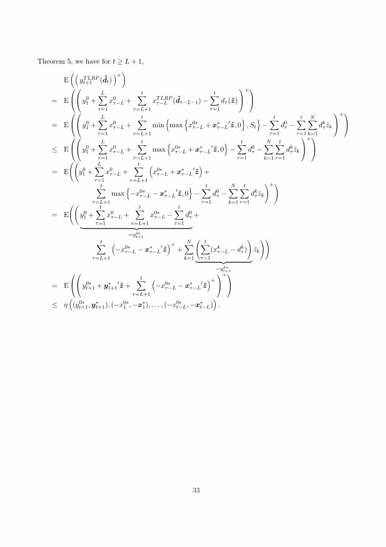
Theorem 5, we have for t ≥ L + 1,

E((

yTLRPt+1 (dt)

)+)

= E

y0

1 +L∑

τ=1

x0τ−L +

t∑

τ=L+1

xTLRPτ−L (dτ−L−1)−

t∑

τ=1

dτ (z)

+

= E

y0

1 +L∑

τ=1

x0τ−L +

t∑

τ=L+1

min{max

{x0∗

τ−L + x∗τ−L′z, 0

}, St

}−

t∑

τ=1

d0τ −

t∑

τ=1

N∑

k=1

dkτ zk

+

≤ E

y0

1 +L∑

τ=1

x0τ−L +

t∑

τ=L+1

max{x0∗

τ−L + x∗τ−L′z, 0

}−

t∑

τ=1

d0τ −

N∑

k=1

t∑

τ=1

dkτ zk

+

= E

((y01 +

L∑

τ=1

x0τ−L +

t∑

τ=L+1

(x0∗

τ−L + x∗τ−L′z

)+

t∑

τ=L+1

max{−x0∗

τ−L − x∗τ−L′z, 0

}−

t∑

τ=1

d0τ −

N∑

k=1

t∑

τ=1

dkτ zk

)+)

= E

((y01 +

t∑

τ=1

x0τ−L +

t∑

τ=L+1

x0∗τ−L −

t∑

τ=1

d0τ

︸ ︷︷ ︸=y0∗

t+1

+

t∑

τ=L+1

(−x0∗

τ−L − x∗τ−L′z

)++

N∑

k=1

(t∑

τ=1

(xkτ−L − dk

τ )

)

︸ ︷︷ ︸=yk∗

t+1

zk

))

= E

y0∗

t+1 + y∗t+1′z +

t∑

τ=L+1

(−x0∗

τ−L − x∗τ−L′z

)+

+

≤ η((y0∗

t+1,y∗t+1), (−x0∗

1 ,−x∗1), . . . , (−x0∗t−L,−x∗t−L)

).

33

Similarly

E((

yTLRPt+1 (dt)

)−)

= E((−yTLRP

t+1 (dt))+

)

= E

−y0

1 −L∑

τ=1

x0τ−L −

t∑

τ=L+1

xTLRPτ−L (dτ−L−1) +

t∑

τ=1

dτ (z)

+

= E

−y0

1 −L∑

τ=1

x0τ−L −

t∑

τ=L+1

min{max

{x0∗

τ−L + x∗τ−L′z, 0

}, St

}−

t∑

τ=1

d0τ +

t∑

τ=1

N∑

k=1

dkτ zk

+

≤ E

−y0

1 −L∑

τ=1

x0τ−L −

t∑

τ=L+1

min{x0∗

τ−L + x∗τ−L′z, St

}+

t∑

τ=1

d0τ −

N∑

k=1

t∑

τ=1

dkτ zk

+

= E

((− y0

1 −L∑

τ=1

x0τ−L −

t∑

τ=L+1

(x0∗

τ−L − x∗τ−L′z

)+

t∑

τ=L+1

(−min

{St − x0∗

τ−L − x∗τ−L′z, 0

})+

t∑

τ=1

d0τ +

N∑

k=1

t∑

τ=1

dkτ zk

)+)

= E

((−y0

1 −L∑

τ=1

x0τ−L −

t∑

τ=L+1

x0∗τ−L +

t∑

τ=1

d0τ

︸ ︷︷ ︸=−y0∗

t+1

+

t∑

τ=L+1

(x0∗

τ−L − St + x∗τ−L′z

)++

N∑

k=1

(t∑

τ=1

(−xk∗τ−L + dk

τ )

)

︸ ︷︷ ︸=−yk∗

t+1

zk

))

= E

−y0∗

t+1 − y∗t+1′z +

t∑

τ=L+1

(x0∗

τ−L − St + x∗τ−L′z

)+

+

≤ η((−y0∗

t+1,−y∗t+1), (x0∗1 − St, x

∗1), . . . , (x

0∗t−L − St,x

∗t−L)

).

34