
Pathways of Early Fatherhood, Marriage, and Employment:...
45
Men’s Early Fatherhood Pathways 1 Running Head: MEN’S EARLY FATHERHOOD PATHWAYS Pathways of Early Fatherhood, Marriage, and Employment: A Latent Class Growth Analysis DO NOT CITE OR QUOTE WITHOUT AUTHOR PERMISSION
Transcript of Pathways of Early Fatherhood, Marriage, and Employment:...

Men’s Early Fatherhood Pathways 1
Running Head: MEN’S EARLY FATHERHOOD PATHWAYS
Pathways of Early Fatherhood, Marriage, and Employment: A Latent Class Growth Analysis
DO NOT CITE OR QUOTE WITHOUT AUTHOR PERMISSION

Men’s Early Fatherhood Pathways 2
Abstract
In NLSY79, young fathers (those with first births earlier than the cohort average) include heterogeneous subgroups with varying early life pathways in terms of fatherhood timing in relation to the timing of first marriage and to holding fulltime employment. Using Latent Class Growth Analysis (LCGA) with 10 observations between age 18 and 37, we empirically derived four latent classes representing different early fatherhood pathways (EFPs): (A) Married Fully-Employed Young Fathers, (B) Married Fully-Employed Teen Fathers,(C) Married Partially-Employed Teen/Young Fathers, and (D) Unmarried Partially-Employed Teen/Young Fathers. Men who become fathers around age 24 (cohort average), following fulltime employment and marriage, a fifth latent class termed On-Time fathers, are the comparison group. About 90% of all early fathers are married, nearly 75% are age 20 or older, and 74.3% hold fulltime employment at the time of the first birth. Even so, with sociodemographic background controlled, all or most early fatherhood groups show subsequent disadvantage in life outcomes (income, educational attainment, incarceration, and number of marriages and children). Nonetheless, as hypothesized, the extent of disadvantage on some outcomes is also greater when early fatherhood occurs at relatively younger age (before age 20), occurs outside marriage, or occurs outside full-time employment.

Men’s Early Fatherhood Pathways 3
BACKGROUND
Many young men today are only loosely attached to their children, their children’s
mothers, and the workforce, coinciding with rising rates of non-marital childbearing, increases in
divorce, increases in the share of children being raised in impoverished female-headed families,
and the failure of some biological fathers to provide economic support to their children.
These trends are a cause for concern because accumulating evidence suggests that
children living in a single parent household, especially one headed by a never-married mother,
can experience substantial negative consequences (including poverty, problems with school,
delinquency, dropping out, failure to go to college, teen parenthood, and employment difficulties
(Cherlin and Furstenberg 1994; Fomby and Cherlin 2007; McLanahan and Sandefur 1994).
Some link these shifts in family life to shifts in the labor force participation of men and women
(Lundberg 2005). For example, several analysts have suggested that changes in marriage can be
partially explained by declines in young men’s ability to establish and maintain stable career
trajectories (Anderson 1990; Oppenheimer et al. 1997).
There are significant gaps in our knowledge about men's roles in childbearing and
marriage decisions, and the links between family and work for men (Oppenheimer, 2003).
Sorting out the interconnections between employment and family patterns is complex because
individuals typically make a number of interrelated transitions as they move out of their teen
years into their twenties. These transitions are often packaged or occur together or in close
proximity and including school completion and entry into the labor market, entry into romantic
unions of various kinds, and the occurrence of pregnancies and births. Surprisingly little
descriptive work has been conducted since Rindfuss (1991) documented both the density and
complexity of the transitions that occur as teenagers grow up in the U.S.

Men’s Early Fatherhood Pathways 4
Early Parenthood
Early motherhood. An extensive body of research has focused on mothers who are
young (Astone and Upchurch 1994; Furstenberg 1991; Geronimus 1994; Jaffee 2002), unmarried
(Wu and Wolfe 2003; Bronars and Grogger 1994), or both (Beutel 2000; Furstenberg et al. 1990;
Moore, Manlove, Glei, and Morrison 1998). These two indicators—early motherhood and
unmarried motherhood—are highly correlated but the nature of the correlation has changed over
time.
There is little research on how women’s work lives are associated with early
childbearing. This is probably because motherhood at any age is known to reduce women’s
labor force attachment and theory does not lead to any obvious a-priori hypothesis about how
this association differs by the age at motherhood. Rather, researchers interested in how early
motherhood affects women’s attainment have focused on educational outcomes (Jones et al.
1999).
Early fatherhood. A much smaller but growing set of studies has also investigated
young fatherhood. This literature has particularly addressed factors associated with teen
fatherhood, and the service needs of teen and young married fatherhood (Lamb and Elster 1986;
Lerman and Ooms 1993; Marsiglio and Cohan 1997; McLanahan and Carlson 2004). Research
usually hypothesizes that young and/or unmarried fatherhood has negative consequences for men
in later life (Garfinkel et al. 2009). This assumption provides part of the rationale for programs
designed to delay young men’s transition to fatherhood, and for interventions fostering marriage
among young unmarried men whose partners become pregnant. As discussed below, several
studies have empirically examined the consequences of teen and/or unmarried fatherhood
(Marsiglio 1987; Nock 1998; Sigle-Rushton 2003. There are a number of “lessons learned” from

Men’s Early Fatherhood Pathways 5
research on young motherhood that researchers could apply, and in many cases have applied, to
research on young fatherhood.
The marital and employment context of first birth. First, research on the association
of young fatherhood with outcomes needs to take into consideration the marital context of the
birth and the timing and sequencing of marriage and parenthood more generally. There is some
evidence that the sequelae of young fatherhood vary by whether the birth is marital or not and
the sequelae of non-marital births depend on age at fatherhood (Marsiglio 1987; Sigle-Rushton
2003). For example, men who were not in a union with their female partners at the time of the
birth had worse outcomes, especially pertaining to employment, than men in unions (Sigle-
Rushton 2003). Further, based on NLSY79 data, only 31 percent men who marry as teenagers
and become fathers within marriage and 63 percent of men who became nonmarital teenage
fathers completed high school (Marsiglio 1987). This is in comparison to 86 percent of peers
who postponed fatherhood past their teenage years. In turn, low school completion leads to
employment and earning disadvantages. Marsiglio (1987) posed the question of how the
relationship context with the child’s mother – marital, cohabiting, non-residential - related to
men’s outcomes (education specifically).
Another important context for early parenthood is employment status, which may be
particularly salient for men given their traditional role as breadwinner with resident children as
well as their concern about financially supporting children with whom they do not live. Some
research examines how fathers’ employment is affected in the years following the birth. But,
studies examining how this varies by fathers’ marital status are recent and rare (Astone et al.,
forthcoming; Garfinkel et al. 2009; Percheski and Wildeman 2008). There is little study about
how a father’s employment status before, at and after the transition to fatherhood moderates the

Men’s Early Fatherhood Pathways 6
association of young fatherhood with later outcomes.
Modeling strategies. One approach to understanding the linkages between marriage,
parenthood and work is to apply various statistical modeling strategies in an effort to simulate
experimental designs. This is the approach taken by econometricians (Upchurch et al. 2001,
2002) and it is essential if the goal is to inform policy makers on how intervening in one area
(e.g. promoting marriage) may impact another (e.g. employment). An alternative is to recognize
that people make decisions about work, family and marriage jointly to some extent, to model
them as simultaneous decisions, and to look at the antecedents and consequences of these joint
decisions. Recent advances in statistical methods make such complex models of the timing and
sequencing of life events possible
For example, recent work explores how marital context relates to employment (Percheski
and Wildeman 2008). Using growth curve models with Fragile Families baseline and five-year
follow-up (after becoming a father) data from 1,084 fathers, Percheski and Wildeman (2008)
report that in the year before becoming a father, married men work more weeks per year and
many more hours per week compared to either cohabiting or non-residential men soon to be
fathers. But, five years later these differences no longer hold as unmarried men increase their
work while married fathers maintain their work levels. When selection variables are controlled,
differences at baseline and five years later no longer exist for the number of weeks worked per
year; yet, married men still maintain a significant lead in hours worked even though their values
diminished. Other research supports the finding the increased work effort (in hours worked) is
associated with becoming a first-time father for unmarried (but not married) men (Astone et al.
forthcoming).
Selection. Another lesson learned from research on young motherhood is that young

Men’s Early Fatherhood Pathways 7
mothers are highly selected. Many studies have established that the associations of young
motherhood with later outcomes for the woman are diminished substantially when selection into
young motherhood is taken into account (Lawlor and Shaw 2002). Second, selection effects
need to be taken into account. Men who become fathers early and/or outside of marriage may
differ markedly from those who do not in their sociodemographic background characteristics.
Prior studies suggest that selection factors account for much of the poorer later life outcomes
experienced by men who become fathers when young and/or unmarried compared to those who
do not, although some differences remain. For example, Sigle-Rushton (2003), using a U.K.
sample of men who become fathers prior to age 22 and a matched sample of older men who had
children or did not become fathers, found that by age 30 early fathers only differed on three
outcomes: public housing subsidies, welfare receipt, and malaise. Men did not differ on
unemployment/ low occupational status. According to Sigle-Rushton childhood disadvantages
contribute to both early fatherhood and its associated negative outcomes. In Nock’s analysis of
later life outcomes associated with unmarried fatherhood in the NLSY 1979, the deficit in
earnings of decreased yearly employment, and increased poverty status of men becoming fathers
under age 20 and between 20 and 25 relative to men over age 26, decreases in magnitude after
controlling for race, family background, and individual characteristics. When men’s relationship
history (ever-married or ever-cohabited) is further added to the models, most of the relationships
between early fatherhood and earnings, employment, and poverty are no longer significant. The
one outcome variable that is robust against these selection variables is educational attainment,
however.
Short versus long term outcomes. The final lesson learned from studies of young
motherhood is that short term consequences and long term consequences of early parenthood

Men’s Early Fatherhood Pathways 8
may be different. For women, it appears that in the years immediately following the birth young
mothers are quite disadvantaged compared to their peers who delay childbearing, but many
resilient young mothers recoup and the differences between them and their peers who delayed
motherhood are not so profound in mid-adulthood (Furstenberg, Brooks-Gunn and Morgan
1987). These findings call attention to the importance, when comparing young fathers to men
who make the transition later in life, making these comparison at more than one stage of the life
course.
Research Questions and Hypotheses
Past research on early parenthood has established that the experience of becoming a
father at a young age varies by whether or not it occurs in marriage, and by the work status of the
father (Astone et al., forthcoming). Focusing on men who become fathers at a relatively young
age, the overall objective of this study is to identify and explore the pathways men take into early
parent, spouse, and worker roles; the sociodemographic background correlates of these
pathways; and their sequelae in later life. Two more specific research questions guide this study.
First, do all young fathers have similar early life pathways? If not, how do their pathways vary
in terms of the timing of first marriage and of their full-time employment status across time, and
how are these varying pathways related to sociodemographic background characteristics?
Second, how are early fatherhood pathways associated with life outcomes in later life
(young adulthood - age 26, and later adulthood - age 37), with sociodemographic background
characteristics controlled? We hypothesize that:
1. Early fatherhood pathways are associated with more disadvantaged later life
outcomes than in pathways in which men transition into fatherhood “on-time ,” in an

Men’s Early Fatherhood Pathways 9
the normative sequence following marriage and fulltime employment (hereafter
termed simply “on-time”).
Among early fatherhood pathways, more disadvantaged later life outcomes are associated with:
2. Pathways characterized by younger median ages of first fatherhood (i.e., before age
20) than in pathways characterized by older median ages at first fatherhood (age 20
or later), as well as on-time pathways.
3. Pathways in which the first birth occurs outside marriage (concurrent or soon
thereafter) than in pathways in which the first birth occurs inside marriage, as well as
on-time pathways.
4. Pathways in which the first birth occurs when the father does not have fulltime
employment (concurrent or soon thereafter) than when he does have fulltime
employment, as well as on-time pathways.
Finally, we also hypothesize that:
5. The later life disadvantages associated with young fatherhood decrease over the life
span as they do for women.
We assess these hypotheses using two types of outcomes. Our primary outcomes of
interest include income, educational attainment, and incarceration, all of which are commonly
agreed upon indicators of disadvantage. Additional outcomes include the number of marriages
and number of children. More marriages and children confer greater financial responsibilities to
support others. If a man experiences lower attachment to the job market, having multiple
children and a divorce may compound his already disadvantaged situation.

Men’s Early Fatherhood Pathways 10
DATA AND METHODS
Sample
The 1979 Cohort of the National Longitudinal Survey of Youth (NLSY79), a nationally
representative sample of youth aged 14 to 21 in 1979, is the data source for this study. These
youth were interviewed annually until 1992 and biennially since then. These analyses are
limited to the “cross-sectional1
The analytic sample differs on some demographic variables relative to the sample of
respondents with missing data for at least one observation from the 10 used in these analyses
(Table 1). The analytic sample is more advantaged in terms of youth poverty, highest
educational attainment, living with both parents at age 14 and less likely to live with step parents,
and less likely to have mothers with less than a high school education. Although the two
samples do not differ with respect to proportion of Black men, they do differ on the proportion of
white and Hispanic men with the analytic sample having more white men and fewer Hispanic
” sample representative of the non-institutionalized civilian
population of young people born from 1957 to 1964. We excluded female respondents and over-
samples of poor respondents resulting in a sample size of 2800 men who were either African
American, European American, or Latino. We examine men’s role trajectories from age 18
through 37, spanning nearly 20 years of development. Given the computational complexity of
analyzing 19 times of measurement, data from ten approximately evenly spaced ages (18, 20, 22,
24, 26, 28, 30, 32, 34, 35, and 37) were used. We restricted the sample to men who provided
data at all 10 ages; the final study sample size is 1,992 men. The demographic characteristics of
the study sample with the full sample are reported in Table 1.
1 This term is used by NLSY79 even though the sample is longitudinal. It is used to distinguish
these respondents from the military and poor subsamples.

Men’s Early Fatherhood Pathways 11
men. Although not addressing selection into the analytic sample, these variables are controlled
in our analyses.
--------------------------------
Insert Table 1 about here
--------------------------------
Variables for Latent Class Analysis
Three binary variables were created for each of the ten ages: ever fatherhood, ever
married, and full-time work status. The distributions reported below pertain to the analytic
sample (N=1992) and are unweighted unless so specified.
Ever fatherhood status. We used birth date information from the respondent’s oldest
child and his own birth date to calculate the respondent’s age at first biological fatherhood. We
coded whether or not each respondent was a father at each age observation used in the analysis.
Respondents who never transitioned into fatherhood by age 37 were coded 0 on this variable for
all observed ages up to 37. Men who became fathers were coded 1 for the age at first fatherhood
and for each subsequent year of age observed up to age 37. For example, if we calculated that a
respondent became a father for the first time at age 19, he was also coded as being a father for
observed ages 20 through 37 (ever a father by age 37: N= 1429; 71.7% of the analytic sample).
We did not take into account infant mortality, so any man whose only child died retained a code
of 1 after the death.
Ever married status. We use a similar strategy for marriage. We pooled data across all
survey years to calculate the date of first marriage for each respondent and used his birth date to
generate his age at first marriage. Respondents who never married were coded 0 for marital
status at all observed ages up to age 37. Respondents who ever married were coded 1 for ever

Men’s Early Fatherhood Pathways 12
married marital status beginning at the observed age of first marriage and beyond up to age 37
(ever married by age 37: N= 1581; 79.4%). Given the construct was ever married, men who
separated or divorced were still coded as 1.
Fulltime work status. We aggregated the weekly labor force activity data to calculate
each man’s median yearly work hours. Men who worked 1,440 hours or more a year (consistent
with working 30 hours per week for 52 weeks) were classified as working fulltime for that year.
For each age, we coded 0 for men who did not meet this criterion for hours worked in the past
year and coded 1 for men who met or exceeded this criterion. Unlike the marital and fatherhood
status variables, fulltime work status is allowed to vary (0 to 1 or 1 to 0) over time from age 18 to
37.
Background Demographic Variables and Covariates
Race/ Ethnicity. Our analyses include men of three racial/ ethnic backgrounds: Whites/
other (non-Hispanic whites, Asian Americans, missing ethnicity), Blacks (non-Hispanic blacks),
and Latinos. The sample consisted of approximately 81.1 percent white, 12.4 percent black, and
6.5 percent Latino male youth.
Highest educational attainment. During each survey year respondents were asked their
highest year of education completed to date. The sample average is 13.3 years of education
(some college).
Youth poverty. We used youth poverty status variables from 1978 and 1979 (1= in
poverty; 0 = not in poverty). These variables were created based on measures of family income
at the time each youth entered the study (ages 14-21). Approximately 10.4 percent of the sample
experienced youth poverty.
Family structure at age 14. In 1979 respondents reported with whom they lived at age

Men’s Early Fatherhood Pathways 13
14. We recoded living arrangements at age 14 into four categories: with both biological parents,
one biological parent only, one biological parent and a stepparent, and no biological parents.
Both biological parents households were the predominant living arrangement at age 14 (77.6%)
followed by biological and stepparent (8.4%), single biological parent (11.9%), and no biological
parents (2.1%).
Mother’s characteristics. Mother’s highest level of educational attainment, a
continuous variable, was collected in 1979. We also use mother’s age at the time of the
respondent’s birth.
Limited work. Beginning in 1979, men reported whether their health limits the kind of
work they can do. If a man reported his work was limited by his health by age 26 and by age 37,
he was coded as being limited in work at that age. If he was disabled or completely unable to
work during any wave, he was coded as ever being disabled (N=332; 16.7% by age 26; N=488;
24.5% by age 37).
Outcomes – Age 26, Age 37, and Lifetime
Respondents’ income at ages 26 and 37. Annual incomes for each survey year were
calculated based on wage data for each respondent. The sample average income was $17,210 at
age 26 and nearly $39,781 at age 37.
Respondents’ highest educational attainment at age 37. Respondents reported their
highest grade of educational attainment at each observation. The sample average was 13.5 years
of education (1.5 years beyond high school).
Number of marriages at age 26 and 37. Men reported the total number of marriages
they experienced at ages 26 and 37. By age 26, nearly half (46.8%) of the sample had never
married, 47 percent were married once, and 5.9 percent were married two times or more. More

Men’s Early Fatherhood Pathways 14
than one-fifth of the sample did not report ever being married by age 37 (20.6%). Over half of
the men reported being married once (56.5%) and 22.9 percent of the sample reported higher-
order marriages.
Number of biological children at ages 26 and 37. Men reported the number of
biological children they had at each observation. By age 26 about two-thirds (62.7%) of the
sample did not have any children, 20.9 percent had one child, 12 percent had two children and
4.4 percent had three or more children. By age 37 over one-fourth had no children (28.3%), 18.9
percent reported one child, 30.6 percent reported having two children, and 22.2 percent reported
having three or more children.
Incarceration: By age 26. Given that the NLSY79 does not contain an item that
directly asks men if they have ever spent time in prison or jail, incarceration by age 26 was
created using residence items from age 18 to 262
Overview of latent class approaches. In principle, Latent Class Analysis (LCA) is akin
. If a man ever reported he was currently
residing in jail or prison, he was coded as having a history of incarceration (N=121; 6.1%). This
by necessity is an underestimate given it is likely that some inmates attrited, and other
respondents who had been imprisoned were not residing in prison when they were interviewed.
Analytic Strategy – Latent Class Analysis
Given the dichotomous nature of status variables and the need to assess trajectories
overtime, we chose a longitudinal categorical data analysis strategy to address our primary
research question.
2 Very few men reported being incarcerated for the first time after age 26 and the number of men
incarcerated between ages 27 and 37 was too small for statistical analyses. Hence, we limit our
analyses to incarceration prior to and including age 26.

Men’s Early Fatherhood Pathways 15
to factor analysis with categorical variables (Lanza & Collins, 2006); how classes of individuals
respond to various items can be thought of as equivalent to factors of items. Traditionally, LCA
has been limited to single points in time and Latent Transition Analysis (LTA) is used to model
the transitions among classes across adjacent time points. One limitation of LTA is that the class
structure at one time point may not be the same as at latter time points even if the same number
of classes is specified. This is also true of factor analysis; three factors may emerge at time 1 and
time 2, but the loadings of specific items may be different for the two time points, resulting in
different definitions and meanings over time. Although LTA has the added advantage of
modeling transitions across time, one may be comparing apples to oranges over time even
though the same overall number of classes is generated for each time point. To avoid both
limitations – so we can model as many time points as possible in the same model to ensure
equivalent meaning – we ran latent class analysis for repeated measures, also known as latent
class growth analysis (LCGA) (Lanza & Collins, 2006; Muthén, 2004).
Latent Class Growth Analysis (LCGA). As applied here, this method empirically
derives varying patterns of the acquisition of roles over the life course, marriage and fulltime
employment, taking into account their sequencing and timing. We initially identify early life
pathways in an LCGA analysis of a full cohort of men rather than just within the subsample of
men who are early fathers for three reasons. First, pathways are defined relative to each other, so
by deriving latent classes in the full sample, early father pathways are defined relative to non-
early-father pathways. Second, rather than setting an arbitrary age cutoff for early fatherhood a
priori (a controversial issue, even more so in light of the “emerging adulthood” concept; Arnett,
2000), we used LCGA to inform how early fatherhood should be defined. Third, empirically
derived (rather than a priori) non-early-father classes can serve as comparisons for the early

Men’s Early Fatherhood Pathways 16
father classes/pathways.
In LCGA, each class represents a pattern of behaviors across the times of measurement
specified in the model (ten times of measurement for this study). In these analyses, we use data
on fatherhood transitions, marital transitions, and fulltime employment status (30 indicators)
over time to derive distinct classes (or subgroups) of men who are homogeneous with respect to
patterns of these indicators over time. In other words, men in the same class have, at each age,
equal probabilities of fatherhood, marriage, and employment in the way defined by the class.
Each LCGA class represents a configuration of both the ordering of the three transitions and the
age at which each transition occurs. For example, two classes might emerge characterized by the
same transition sequencing (e.g., fulltime work followed by marriage and then fatherhood) but
different timing and/or different spacing (one during the mid-20s that spans 10 years and the
other during the mid-30s that spans five years).
At each time point, with three variables,, there are eight possible combinations of statuses
(no transitions, fulltime work only, marriage only, fatherhood only, work and marriage, work and
fatherhood, marriage and fatherhood, and all three statuses). The total number of possible
combinations across all ten time points is 810. Backward transitions (e.g., scored 1 for having
made the transition to fatherhood at age 20 but scored 0 at later ages) are excluded. Even with
these exclusions, the number of theoretically possible combinations is unmanageably large.
LCGA reduces these combinations into a smaller number of latent classes representing common
patterns of the ordering of first fatherhood, first marriage, and fulltime employment over the
period from age 18 to age 37, taking into account timing and spacing as well.
Model estimation. The current analyses were conducted using Proc LCA for SAS 9.1.
Given the difficulty of handling missing data in LCGA models, listwise deletion was used based

Men’s Early Fatherhood Pathways 17
on the three variables of interest over time (marital, fatherhood, and fulltime work status).
Analytic Strategy – Linear and Logistic Regression
For continuous outcome measures, we use linear regression to determine whether latent
class (interpreted here as pathways) predict outcomes after controlling for covariates. For the
dichotomous outcome (incarceration) we use logistic regression.
RESULTS
Are There Distinct Pathways of Early Fatherhood?
The Akaike Information Criterion (AIC) and Bayesian Information Criterion (BIC) for
LCGA models with different numbers of classes were used to determine the best fitting model.
The model with 12 classes3
Serving as a comparison group for many of the analyses is the large latent class termed
here On-Time On-Sequence Fathers (hereafter, On-Time Fathers; 17.0% of the sample). In this
had the best fit (AIC = 10518.7, BIC = 12595.1, compared to values
of 10713.7 and 12616.6 for the 11 class model, and of 10719.3 and 12969.3 for the 13 class
model), and was also the most interpretable.
The median age at first fatherhood for four classes was lower than the median age of first
fatherhood (26.4) in the National Survey of Family Growth (NSFG) 2002 for men of this same
cohort. These four groups thus constitute four empirically derived pathways of early fatherhood
in relation to the timing of marriage and full-time employment. These four classes constitute
37.9% of the sample.
3 This paper does not discuss the seven other latent classes in the LCGA . Four additional
classes represent men who postpone fatherhood, two classes define men who forego fatherhood,
and one class characterizes on-time single fathers. For ease of presentation, we only show the
four classes for early fatherhood and the on-time on-sequence reference class.

Men’s Early Fatherhood Pathways 18
class, men’s transitions occurred in the normative sequence (work, marriage, fatherhood) and at
almost exactly the median ages observed for this cohort in the NSFG2002.
For each early life pathway as well as the On-Time fathers, proportions are reported in
Table 2 and graphically depicted in Figure 1 with values for first fatherhood, first marriage, and
fulltime employment at each age observation.
--------------------------------------------------
Insert Table 2 & Figure 1 about here
--------------------------------------------------
Class A. Married Fully-Employed Young Fathers (19.1% of full sample; 50.4% of
early fathers). Nearly one in five men in the entire sample take the Married Fully-Employed
Young Fathers pathway. Half of the men who take this pathway are fathers by age 23.5; this is
about 4.5 years younger than On-Time fathers. Half of these men work fulltime from age 19.6
onward; so men are typically working when they become dads and they have been working for
four years on average. Few of these men have children prior to age 20. Marriage and fatherhood
are sequenced in that order. These men differ from the On-Time men is that they 1) start these
role transitions (beginning with fulltime employment) early relative to the average, and 2)
proceed through the role transitions relatively quickly, that is, have shorter intervals between role
transitions.
Class B. Married Fully-Employed Teen Fathers (9.2% of full sample; 24.3% of
early fathers). Men in this second most frequent early life pathway have their first children at
the earliest of any of the four early fatherhood classes. Seventy percent have a birth prior to their
20th birthday. These men typically marry prior to the first birth, but the interval between
marriage and birth is quite short (ages differing by 0.6). In addition, these fathers engage in

Men’s Early Fatherhood Pathways 19
fulltime employment coincident with first birth, rather than prior to it as in class A.
Class C. Married Partially-Employed Teen/Young Fathers (5.2% of full sample;
14.0% of early fathers). Half of men in this early life pathway have their first child by age
21.2. Thirty percent have their child before age 20 and 70% do so after. Pathway C men marry
nearly simultaneously with their first birth which suggests that for many, marriage might be
triggered by the pregnancy. The distinctive feature of this pathway is the low rates of fulltime
employment; this rate does not rise above 20 percent through their early 20s, and peaks at only
50 percent from age 29 to age 37.
Class D. Unmarried Partially-Employed Teen/Young Fathers (4.4% of full sample;
11.6% of early fathers). This final pathway straddles 20 as the age at which half report a first
birth; about 45% report first birth prior to age 20. The first distinctive feature of this early life
pathway is that members show higher rates of fulltime employment at earlier ages, reaching 50
percent by age 23 and remaining stable at nearly 60 percent though their 30s. Second, this
pathway has the lowest rate of marriage, with no members reporting a marriage until after age
28, with less than 30 percent marrying by age 37. It is possible that many of these marriages are
to a woman other than the mother of their oldest child.
On-Time Fathers (17.0% of full sample). The On-Time father pathway evinces
median ages of first fatherhood, first marriage, and rates of fulltime work close to the medians
observed in the NSFG2002 for men aged 38 to 42 (same cohort as NLSY79 men; author
calculations). These men are “normative” in two respects: the timing and the sequencing of role
transitions. Focusing specifically on On-Time fathers, the age by which half of men have
entered fatherhood is approximately 28; similarly the age by which half of men have married for
the first time is nearly 25 and the age by which half are currently employed fulltime is slightly

Men’s Early Fatherhood Pathways 20
older than age 21. Furthermore, these men follow the normative sequence of working prior to
marriage and marrying prior to becoming fathers. On-Time men serve as our comparison group
rather than all men or all fathers. This strategy protects us from mistaking high levels of
attainment by men who delay fatherhood for disadvantage among young fathers.
Do Men Who Take These Different Pathways Differ on Background Characteristics?
We assessed bivariate associations between early life pathway and four
sociodemographic background characteristics (race-ethnicity, youth poverty status, living
arrangements at age 14, mother’s education). The results are reported in Table 3.
--------------------------------
Insert Table 3 about here
--------------------------------
All Early Fatherhood Pathways versus On-Time Fathers. Table 3 shows that when
the men in all Pathways are pooled (top panel, row 3), and contrasted with the reference group
(row 2), they are more likely to be ethnic minorities (although the percent Hispanic does not
reach statistical significance) and more likely to be disadvantaged (in terms of youth poverty,
family constellation at age 14, maternal education)4
Individual Early Fatherhood Pathways and On-Time Fathers. Turning to specific
pathways and their association with these demographic characteristics, we find heterogeneity
among pathways. With respect to race-ethnicity, pathways C and D have high proportions of
. These differences are apparent whether the
comparison is with all men or with the On-Time men.
4 Multiple group comparisons with Tukey adjustments were used for these bivariate analyses.
Classes that do not share any common superscripts are statistically significantly different from
each other.

Men’s Early Fatherhood Pathways 21
racial-ethnic minorities (i.e., significantly different from On-Time fathers, and from pathways A
and B). Pathways C consists of 22.1 percent black men and over half of pathway D are black
men.
In terms of youth poverty, the same two pathways also have high rates (over one-third of
pathway D and one-sixth of pathway C). Similar to the findings for youth poverty, the lowest
percent of men who lived with both parents at age 14 are reported by pathways D (58%) and C
(60%). Mother’s education is the only sociodemographic variable reported in Table 3 for which
all four pathways report significantly lower values relative to On-Time fathers, with pathway A
men reporting nearly one year less and other pathway men reporting 1.5 years less of maternal
education. On average, men from all four pathways report their mothers earned less than a high
school education with three reporting less than eleventh grade attainment for their mothers.
In contrast to the findings for combined pathways, the differences among pathways are
notable with men on pathways C and D coming from more disadvantaged backgrounds than On-
Time fathers. Pathway D also differs significantly from pathways A, B, and C with respect to
race and youth poverty, and differ from pathways A and B in terms of living arrangements at age
14.
How Are Early Fatherhood Pathways Associated with Later Life Outcomes?
We test hypotheses concerning the later life disadvantages associated with young
fatherhood in general (H1)5
5 H1, H2, H3, H4, H5 refer to hypotheses 1-5 described earlier. This shorthand will be used
from this point forward.
, concerning the role of age (H2), marital (H3), and employment (H4)
contexts in these disadvantages, and concerning decreasing disadvantage over the life span (H5).
As observed above, men in all early father pathways pooled together are more likely to be ethnic

Men’s Early Fatherhood Pathways 22
minorities and to have disadvantaged backgrounds (youth poverty, family constellation at age 14,
and maternal education). In addition, pathways C and D also include significantly higher
proportions of racial-ethnic minorities, and more often report youth poverty, not living with both
parents at age 14, and lower levels of maternal education attainment than do pathways A and B.
Thus, it is evident that there are important processes of selection into the different pathways that
need to be controlled for in all analyses.6
Tables 4-6 analyze how the four early fatherhood pathways compare to On-Time fathers
(H1), and Table 7 provides additional comparisons of the four early fatherhood pathways with
each other, in all cases with sociodemographic background controlled . We review the results in
light of the hypotheses, making several different comparisons. First, we compare each early
fatherhood pathway to On-Time fathers to test whether men with early transitions differ from the
latter (H1). Next we compare pathway B to A given these pathways differ primarily in terms of
the timing of fatherhood, not its work and marital context (H2). We then compare pathways C
and D since their timing of fatherhood is the same, but the marital context differs (H3). Next, we
compare pathways A and B to pathways C and D, since the two sets of pathways differ in the
Although we control for typical selection variables, we
recognize that unmeasured selection effects may still exist.
6 For each outcome in Tables 4-6 we report three regression models. Model 1 depicts the rela-
tionship between each pathway and the outcome of interest with no other variables. Only soci-
odemographic variables are used to predict the outcome in Model 2. Both pathways and soci-
odemographic variables predict the outcome in Model 3, thereby representing the unique contri-
bution of each variable above and beyond the other variables in the model. Differences in R-
squares from Model 2 and Model 3 for continuous variables denote whether the addition of
pathways to the model significantly improves the model.

Men’s Early Fatherhood Pathways 23
employment context of first fatherhood (H4; though varying in age and marital context). For
H2-4, detailed pairwise comparisons of pathways with each other and with On-Time Fathers are
presented. Finally, we assess whether disadvantages associated with early fatherhood decrease
from age 26 to 37 by comparing results for age 26 outcomes with those for age 37 outcomes
(H5).
How Early Fatherhood Pathways Compare to On-Time Fathers (H1)
According to Hypothesis 1, early fatherhood pathways will report disadvantages in later
life outcomes relative to On-Time fathers; recall that in this latter pathway, fatherhood occurs in
the mid-twenties followed fulltime employment and marriage. Results for income7
In terms of educational attainment by age 37, all four pathways also show lower levels of
and
education are reported in Table 4. By age 37 men on all four pathways report significantly lower
incomes ($6,000-$28,000 lower) relative to On-Time men. Compared to On-Time fathers, two of
the four pathways report lower earnings at age 26. Men on pathways C and D reported
significantly lower incomes ($9,000-$13,700 lower) than On-Time men (Table 4). In monetary
terms, after controlling for sociodemographic variables including work limitations and region,
pathway C men earn nearly $14,000 less a year and pathway D men earn over $9,000 less a year
relative to On-Time fathers.
-----------------------------------------
Insert Tables 4, 5, 6 about here
-----------------------------------------
7 Both log-income and income were modeled. Analyses determined that log-income models did
not fit the data any better than income in dollars models. For ease of interpretation, only in-
comes in dollars for both ages 26 and 37 are presented in Table 4.

Men’s Early Fatherhood Pathways 24
education relative to On-Time men, by 1.1 - 1.8 years (Table 4). Three of the four early father
pathways (A, B, C) report more marriages at age 26, though only two do so at age 37 (B and C;
Table 5). All early father pathways report more children at age 26 (1.2-1.8; p<0.001) with men
having children at the youngest ages (B) reporting the largest difference (almost two more
children by age 26 than On-Time men), and three do so at age 37 (A, B, C; 0.35-0.53; p < 0.05).
There is least support for H1 for incarceration at age 26 with less than 1.5% of men on
pathways A and B and On-Time men report incarceration by age 26. Two pathways (C and D;
Tables 6), however, are characterized by significantly higher histories of being incarcerated
relative to On-Time men (2.0-3.2 odds ratios, p < 0.05). In sum, men who transition early into
fatherhood report lower incomes, less educational attainment, more marriages and children, and
more incarceration (for two groups) relative to their On-Time peers, controlling for background
factors.
It is important to note that selection differences explain some, but not all, of the observed
disadvantage of young age at first fatherhood. For each outcome, models including demographic
variables only (Models 2 in Tables 4 and 5) are improved with the addition of pathways (Models
3 in Tables 4 and 5) as evinced by significant changes in R-squares. Hence, early fatherhood
pathways independently and uniquely influence outcomes of interest above and beyond
sociodemographic variables.
How Relatively Younger Age at First Birth Relates to Disadvantaged Outcomes (H2).
We hypothesize- that among early fathers, becoming a father at a relatively younger age,
e.g., before age 20, is associated with greater disadvantage. Among early fathers, pathway A
(Married Fully-Employed Young Fathers) and pathway B (Married Fully-Employed Teen
Fathers) differ on how early the transition into fatherhood occurs (as teens, or in early 20’s),

Men’s Early Fatherhood Pathways 25
while being similar in the marital and employment context of first births. Differences among
these two pathways hold after controlling for confounders (Table 7). Those men with first births
at relatively younger ages report lower income at both age 26 (ns) and age 37 ($8,000 lower, p <
0.05). In addition, men on pathway B report three-quarters of a year less educational attainment
relative to men on pathway A.
--------------------------------
Insert Table 7 about here
--------------------------------
Men who transition earlier (B) report significantly higher numbers of marriage at both
age 26 (p < 0.05) and age 37 (p < 0.05). Men who transition earlier (B) report significantly
higher number of children relative to men who transition later (A) at age 26 (1.9 versus 1.3,
respectively; p < 0.05) and age 37 (2.7 versus 2.5; p < 0.05). In short, among men who are both
married and fully employed at the time of a first birth, men who transition into fatherhood earlier
(B) report more disadvantage in terms of income, education, number of marriages, and number
of children relative to their postponing peers (A).
How the Marital Context of First Births Relates to Disadvantaged Outcomes (H3)
We hypothesize that pathways characterized by nonmarital early births will be associated
with more disadvantaged outcomes. All men of pathway D become fathers before marrying. By
definition, these men report significantly lower number of marriages than the three other
pathways and On-Time men. Hence, we will focus on the other outcomes of interest.
Unmarried fathers (D) report less income at age 26 and 37 compared to On-Time men ($9,000
compared to $28,000; Table 4). Men of pathway D also report significantly lower incomes
relative to pathways A and B – both characterized by marital first births - at ages 26 and 37

Men’s Early Fatherhood Pathways 26
($8,000-9,000 and $14,467-22,457 lower, respectively, Table 7). Compared to their married
partially-employed father counterparts, pathway C men, the income of pathway D is significantly
higher at age 26 but not significantly different at age 37 (although it is lower at age 37).
By age 37 men of pathway D report 1.8 fewer years of educational attainment relative to
On-Time men (p < 0.001). Furthermore, of all early fatherhood pathways, men in pathway D
report the lowest level of education but only differ significantly from pathway A (Table 7).
By age 26, men reporting nonmarital first births (D) report higher numbers of children
compared to On-Time men (1.2, p < 0.01). By age 37, however, the difference reverses whereby
men of pathway D report marginally fewer children than On-Time men (ns) and the three
remaining early fatherhood pathways (Table 7).
One potential explanation for the lack of marriages and fewer numbers of children for
pathway D men at age 37 is high incarceration by age 26. Relative to On-Time men, pathway D
men are 3.2 times more likely to have been incarcerated by age 26 (p < 0.001). Nearly one-in-
four pathway D men (23.9%) report being incarcerated by age 26, making this group
significantly higher than all three remaining pathways (the next closest is C with 8.7%).
In sum, men who transition into nonmarital first fatherhood report lower incomes at ages
26 and 37 relative to On-Time men and all three pathways defined by marital fatherhood at age
26 and two of these pathways (A and B) at age 37. Furthermore, pathway D men are
significantly more likely to experience incarceration by age 26 relative to On-Time men and men
of the three marital-birth early fatherhood pathways. Results for educational attainment and
number of children are mixed although pathway D men report the lowest education levels of all
pathways and On-Time men.
How the Employment Context of First Births Relates to Disadvantaged Outcomes (H4)

Men’s Early Fatherhood Pathways 27
We hypothesize men who work less than fulltime (concurrently or soon after the birth)
report greater lifetime disadvantage relative to men who work fulltime before and during the
time of the birth. In other words, we expect men on pathways C and D (both partially-employed
Teen/ Young Fathers) will fare worse than On-Time men and pathways A and B (fully-employed
men at first births) in terms of income, educational attainment, incarceration, number of
marriages, and number of children. We expect these patterns given pathway C and D men are
underemployed.
As shown in Table 4, at ages 26 and 37, men of pathways C and D (both partially
employed fathers) earn significantly less income relative to On-Time men. The gap widens
substantially by age 378
At both ages 26 and 37, pathway C men report significantly greater number of marriages
(0.37 and 0.26 respectively, p < 0.001) and pathway D men report significantly lower number of
marriages (-0.7 and -0.9 respectively, p < 0.001) relative to On-Time men (Table 5). Married
fully-employed young fathers (A) report significantly fewer marriages than pathways B and C by
age 37 (Table 7). These patterns may be partially attributable to the attractiveness of stable and
high employment of men to women. Money concerns are most often cited as the impetus for
. Pathway D men earn nearly twice as much as pathway C men at age
26. By age 37, however, men of these two pathways (C and D) do not significantly differ from
each other in income. These partially employed fathers do significantly differ from their fully
employed peers – pathways A and B – at ages 26 and 37 (Table 7).
In terms of highest educational attainment by age 37, both pathways C and D report
lower education levels by at least one year relative to On-Time men (Table 4) but they do not
significantly differ from each other or pathway B men (Table 7).
8 We acrecognize that inflation may partially explain the increase in the difference.

Men’s Early Fatherhood Pathways 28
divorce (Amato & Previti, 2003) and earnings are considered a valuable characteristic when
seeking a martial partner (Edin & Reed, 2005; Sprecher, Sullivan, & Hatfield, 1994).
At age 26, men of both partially-employed pathways reported significantly higher
numbers of children compared to On-Time men (1.2-1.6; p<0.001). At age 37, only pathway C
men maintained this lead (0.5 children, p < 0.001). Relative to the other early fatherhood
pathways, at age 26 pathway C and D men had moderate numbers of children. By age 37,
pathway D men reported the fewest children and pathways B and C men reported the highest
number of children.
As noted earlier, pathway C and D men report significantly higher levels of incarceration
by age 26 relative to On-Time men (2.0 and 3.2 times higher, p < 0.001). Furthermore, given 24
percent of pathway D men and 9% of pathway C men experienced incarceration (Table 7), they
are substantially more disadvantaged on this outcome relative to pathways A (1.3%) and B
(1.2%).
In sum, partially-employed first-time fathers earn less income and report greater
likelihoods of incarceration relative to their On-Time and pathway A and B peers. Furthermore,
partially-employed men report less educational attainment than On-Time men. This confirms
that partially-employed early fathers experience greater disadvantage than fully-employed peers
on two important variables.
Decreasing Disadvantage Associated with Early Fatherhood Over the Life Span (H5)
Age 26 outcomes. By age 26 our multivariate regression analyses reveal that pathway A
appears more advantaged, earning income comparable to On-Time fathers, supporting fewer
children, and experiencing less marital dissolution. Pathways B, however, reports the highest
number of marriages and children by age 26 of all pathways. Turning to the more disadvantaged

Men’s Early Fatherhood Pathways 29
men at age 26, pathway C and D men significantly differ from On-Time fathers by earning far
less income, fathering more children, completing less schooling, and experiencing jail. Pathway
C men fare worst in terms of earning the least amount of money on which to support a relatively
high number of children in the context of experiencing moderate marital dissolution. Pathway D
men are not far behind in their lower earnings and a higher incarceration history.
Age 37 outcomes. By age 37 men on all pathways earn less income than On-Time
fathers. Pathway A men earn $6,000 less and pathway B men earn $13,300 less. Pathway C and
D men report at least $25,000 less than On-Time fathers. Similar to findings for age 26, pathway
A men appear most advantaged of the pathways. Of the remaining three pathways, pathway B
and C men experience similarly high numbers of children, but pathway B men report a greater
deficiency in educational attainment and greater marital dissolution relative to On-Time fathers
than pathway C men. But, pathway C men have other problems with less income and
employment and just as many children to support (in addition to an incarceration history).
Although pathway D men have the fewest number of children by age 37, they also make the least
amount of money, have the lowest level of educational attainment, and tend to marry less than
other men (perhaps attributable, in part, to incarceration history and employment difficulties). In
sum, the outcomes experienced by early fathers are worse at age 37 than at age 26 when
compared to On-Time fathers.
DISCUSSION
This study documents and describes how young fathers sequence and interconnect work,
marriage, and fatherhood roles, how these patterns vary across sociodemographic subgroups ,
and the later life sequelae of these patterns. Specifically, we employ a latent variable analysis
technique – Latent Class Growth Analysis (LCGA) – to jointly model these processes. A

Men’s Early Fatherhood Pathways 30
methodological limitation of the study is that the use of 10 observations per case led to
considerable attrition in the analysis sample, with important sociodemographic background
differences between the retained and attrited subgroups. Although not addressing this selectivity,
these socioeconomic characteristics are controlled in the analysis. A compensating strength of
the study is its use of NLSY data.
In this study we used LCGA to identify distinct pathways to fatherhood, marriage and
work for men. We identified 12 pathways, of which four constitute pathways to early fatherhood
(37.9% of the sample), that is, first fatherhood earlier than the median age of first fatherhood in
the National Survey of Family Growth (NSFG) 2002 for men of this same cohort. About a
quarter of early fathers were teens at first birth (pathway B, 24.3% of young fathers), with three-
quarters age 20 or older, but still younger than the median age of first fatherhood. Most early
fathers are married when the oldest child is born (A, B, and C, comprising together 88.7% of
early fathers). About three-quarters of early fathers hold full-time employment at the time of
first birth (A and B, 74.3%).
While we partially confirm prior research that with sociodemographic background
controlled, early fatherhood results in subsequent disadvantage, we also find that the extent of
disadvantage on some outcomes varies according to the marital and employment context of the
early birth. Partially confirming our first hypothesis, all or most early fatherhood pathways are
disadvantaged compared to On-Time fathers on the majority of outcomes. Confirming our
second hypothesis that early fatherhood at a relatively younger age (before age 20) is associated
with greater disadvantage, we found that even among young fathers who follow the normative
sequence of work, marriage, and fatherhood, a teenage birth (pathway B) is associated with more
disadvantage than a birth in the early 20s (pathway A).

Men’s Early Fatherhood Pathways 31
Our results also confirm our hypotheses that men who become fathers at relatively
younger ages, outside of marriage, and without fulltime employment report greater disadvantage
relative to their married and fully employed peers, respectively. Those becoming fathers at
relatively younger ages report lower income at both age 26 and 37, and less education at age 37.
Unmarried fathers (pathway D) report lower income at both age 26 and 37 and less educational
attainment. Pathways C and D include attenuated attachment to the labor force which in turn is
related to lower income. There is some evidence that this low labor force attachment is due to
involvement in criminal activity.
In contrast to early motherhood, the disadvantage associated with young fatherhood
increases with age. It appears that compared to On-Time fathers, the outcomes experienced at
age 37 are worse than those outcomes at age 26. The effects of early fatherhood are cumulative
and men do not recover over time. There are important differences in the way that parenthood
affects labor force attachment for men compared to women that may help explain why men show
less recovery from early parenthood than do women. Women of all ages are likely to reduce
their work effort at first birth and while their children are very young and then gradually increase
their work effort as their children grow older (Glauber 2007). If women in their thirties are
compared to each other, for example, it is possible that differences in economic outcomes (labor
supply, wages, work effort) between young mothers and on-time/late mothers will be quite small.
This is because the children of young mothers are, on average, older than the children of on-
time/late mothers and are causing less of a conflict between work and family roles.9
9 It is possible that in mid-life and the older years, when all women’s children are grown, eco-
nomic differences between young mothers and on-time older mothers will re-emerge as a result
of lower levels of education among young mothers.
For men,

Men’s Early Fatherhood Pathways 32
however, parenthood typically intensifies work effort (Glauber 2008). It is possible that early
fatherhood limits the acquisition of human capital either by interrupting education, or preventing
fathers from putting in the extra efforts (overtime, residential moves) to acquire human capital at
work, and that young fathers do not recoup these losses.
In conclusion, the study finds that, with sociodemographic background factors controlled,
all early fatherhood pathways are associated with later life disadvantages on some outcomes. At
the same time, the research also establishes that early fathers are a heterogeneous group, only
minorities of whom at the time of first birth are teens, or are unmarried, or are not fully
employed. As hypothesized, later life disadvantage on many outcomes occurs primarily when
early fatherhood occurs in non-marital context, and when it occurs outside the context of fathers’
full-time employed. These findings apply to a cohort of men who were teenagers in 1979. It is
unclear whether these patterns would emerge in younger cohorts. The findings, however,
suggest that intervention strategies addressing the needs of early fathers need to take into account
both the commonalities and the differences among their heterogeneous subgroups.

Men’s Early Fatherhood Pathways 33
REFERENCES Alan Guttmacher Institute. 2002. “Teen pregnancy: trends and lessons learned.” Available
online at: http://www.guttmacher.org/pubs/tgr/05/1/gr050107.html. Retrieved 19
August 2008.
Amato, P.R. and D. Previti. 2003. “People's reasons for divorcing: Gender, social class, the life
course, and adjustment.” Journal of Family Issues 24: 602-626.
Arnett, J.J. 2000. “Emerging adulthood. A theory of development from the late teens through the
twenties.” American Psychologist 55:469-80.
Astone, N.M. and D. Upchurch. 1994. “Forming a Family, Leaving School Early and Earning a
GED: A Racial and Cohort Comparison.” Journal of Marriage and the Family 56:759-
771.
Bachrach, C. and F.L. Sonenstein. 1998. "Male Fertility and Family Formation: Research and
Data Needs on the Pathways to Fatherhood." Pp. 45-98 in Nurturing Fatherhood:
Improving Data and Research on Male Fertility, Family Formation and Fatherhood,
edited by Federal Interagency Forum on Child and Family Statistics. Washington D.C.:
U.S. Department of Health and Human Services.
Beutel, A.M. 2000. “The Relationship between Adolescent Nonmarital Childbearing and
Educational Expectations: A Cohort and Period Comparison.” The Sociological
Quarterly 41:297-314.
Bronars, S.G. and J. Grogger. 1994. The Economic Consequences of Unwed Motherhood:
Using Twin Births as a Natural Experiment. The American Economic Review 84:1141-
1156.
Hamilton, B.E., J.A. Martin, and S.J. Ventura, S.J. 2007. “Births: Preliminary data for 2006.”

Men’s Early Fatherhood Pathways 34
National Vital Statistics Reports 65. Hyattsville, MD: National Center for Health
Statistics.
Cooney, T.M., F.A. Pedersen, S. Indelicato, and R. Palkovitz. 1993. “Timing of fatherhood: Is
“on-time” optimal?” Journal of Marriage and Family 55:205-215.
Edin, K. and J.M. Reed. 2005. “Why Don't They Just Get Married? Barriers to Marriage among
the Disadvantaged.” The Future of Children 15(2):117-137.
Eggebeen, D. and D. Litcher. 1991. “Race, family structure, and changing poverty among
American Children.” American Sociological Review 56:801-817.
Furstenberg, F.F. 1991. “As the pendulum swings: Teenage childbearing and social
concern.” Family Relations 40: 127-138.
Furstenberg, F.F., L.A. Levine, and J. Brooks-Gunn, J. 1990. “The children of teenage
mothers: Patterns of early childbearing in two generations.” Family Planning
Perspectives 22: 54-61.
Furstenberg, F.F. 1976. Unplanned Parenthood: The Social Consequences of Teenage
Childbearing. New York: Free Press.
Geronimus, A. and S. Korenman. 1992. “The socioeconomic consequences of teen childbearing
reconsidered.” Quarterly Journal of Economics 107:1187-1214
Glauber, R. 2007. "Marriage and the Motherhood Wage Penalty Among African Americans,
Hispanics, and Whites." Journal of Marriage and Family 69:951-961.
Glauber, R. 2008. "Race and Gender in Families and at Work: The Fatherhood Wage Premium."
Gender & Society 22:8-30.
Hamilton, B.E., P.D. Sutton and S.J. Ventura. 2003. “Revised birth and fertility rates for the
1990s: United States, and new rates for Hispanic populations, 2000 and 2001.” National

Men’s Early Fatherhood Pathways 35
Vital Statistics Reports 51(12). Hyattsville, MD: National Center for Health Statistics.
Hardy, J.B. and A.K. Duggan. 1988. “Teenage fathers and the fathers of infants of urban,
teenage mothers.” Am J Public Health 78:919–922.
Meyer VF. 1991. “A critique of adolescent pregnancy prevention research: the invisible white
male.” Adolescence 26:217–222.
Jaffee, S. R. 2002. “Pathways to adversity in young adulthood among early childbearers.”
Journal of Family Psychology 16:38-49.
Lamb, M.E. and A. Elster. 1986. Adolescent fathers. Mahwah, NJ: Erlbaum Associates
Lanza, S.T. and L.M. Collins 2006. “A mixture model of discontinuous development in heavy
drinking from ages 18 to 30: The role of college enrollment.” Journal of Studies on
Alcohol 67: 552-561.
Lerman, R.I. and T.J. Ooms (Eds.). 1993. Young unwed fathers: Changing roles and emerging
policies. Philadelphia: Temple University Press.
Mariglio, W. 1987. “Adolescent fathers in the United States: Their initial living arrangements,
marital experience, and educational outcomes.” Family Planning Perspectives 19:240-
251.
Marsiglio W. and M. Cohan 1997. “Young fathers and child development.” M. E. Lamb (Ed.),
The role of the father in child development, 3rd ed. (pp. 227-244). New York: Wiley.
McLanahan, S. and G. Sandefur. 1994. Growing Up with a Single Parent: What Hurts, What
Helps. Cambridge, MA: Harvard Univ. Press
McLanahan, S. and M.S. Carlson. 2004. “Fathers in fragile families.” In M. E. Lamb (Ed.), The
role of the father in child development, 4th ed. (pp. 222-271). New York: Wiley.
Moore, K.A., J. Manlove, D.A. Glei, and D.R. Morrison. 1998. “Nonmarital school-age

Men’s Early Fatherhood Pathways 36
motherhood: Family, individual, and school characteristics.” Journal of Adolescent
Research 13:433-457.
Muthén, B. 2004. “Latent variable analysis: Growth mixture modeling and related techniques for
longitudinal data.” In D. Kaplan (ed.), Handbook of Quantitative Methodology for the
Social Sciences. Newbury Park, CA: Sage Publications.
Nock, S. 1998. “The consequences of premarital fatherhood.” American Sociological Review
63:250-263.
Oppenheimer, V.K. 2003. “Cohabiting and Marriage during Young Men's Career-Development
Process.” Demography 40:127-149.
Percheski, C. and C. Wildeman. 2008. “Becoming a dad: Employment trajectories of married,
cohabiting, and nonresident fathers.” Social Science Quarterly 89:482-501.
Sigle-Rushton, W. (2003). “Youth fatherhood and subsequent disadvantage in the United
Kingdom.” Journal of Marriage and the Family, 67:735-753.
U.S. Census Bureau. 2005. “Current Population Survey, March and Annual Social and Economic
Supplements, 2005 and earlier”.
Ventura, S.J. and C.A. Bachrach.2000. “Nonmarital childbearing in the United States, 1940–99.”
National Vital Statistics Reports 48(16). Hyattsville, MD: National Center for Health
Statistics.
Woodward, L., D.M. Fergusson, and L.J. Horwood. 2001. “Risk factors and life processes
associated with teenage pregnancy: Results of a prospective study from birth to 20
years.” Journal of Marriage and Family 63:1170-1184.
Wu, L.L. and B.B. Wolfe (Eds.) 2001. Out of wedlock: Causes and consequences of nonmarital
fertility. New York: Russell Sage.

Men’s Early Fatherhood Pathways 37
Table 1. Demographic Characteristics for Analytic and Attrited Samples Analytic Sample Attrited Sample p Demographic Characteristics (N=1992) (N=808) Respondent Characteristics Youth poverty (% yes) 10.4 14.2 0.006 Age at Study Start (mean years) 17.5 17.4 ns Highest Education (mean years) 13.5 13 0.0001 Respondent's Race/ Ethnicity Black (%) 12.4 12.3 ns White (%) 81.1 76.7 0.009 Hispanic (%) 6.5 11 0.0001 Family Structure at age 14 Live with Both Parents (%) 77.5 72.3 0.004 Live with Only One Parent (%) 8.4 7.7 ns Live with Parent and Step Parent (%) 11.9 17.2 0.0002 Live on Own/ Other (%) 2.1 2.6 ns Mother's Characteristics Mother age at birth of respondent (mean years) 44.1 43.9 ns Mother education less than HS (%) 32.2 36.6 0.02 Mother education HS (%) 47.4 44.4 ns Mother education more than HS (%) 20.4 18.9 ns Mother's highest educational attainment (mean years) 11.8 11.5 ns

Men’s Early Life Pathways 38
Table 2. Proportions with first fatherhood, first marriage, and fulltime work at each age, for four Early Fatherhood Pathways , and for On-Time On-Sequence Fathers
Proportion in Each Role Sample Percent (N)
Early Fatherhood Pathway age 18 20 22 24 26 28 30 32 35 37 A. Married fully-employed young fathers
father 0.00 0.02 0.19 0.61 0.93 1.00 1.00 1.00 1.00 1.00 marriage 0.01 0.16 0.62 0.91 0.97 1.00 1.00 1.00 1.00 1.00 19.1 (380) work 0.22 0.59 0.79 0.92 0.93 0.94 0.95 0.94 0.95 0.94
B. Married fully-employed teen fathers
father 0.23 0.70 1.00 1.00 1.00 1.00 1.00 1.00 1.00 1.00 marriage 0.35 0.95 0.98 0.99 1.00 1.00 1.00 1.00 1.00 1.00 9.2 (184) work 0.26 0.67 0.86 0.85 0.92 0.90 0.88 0.91 0.88 0.88
C. Married partially-employed teen/young fathers
father 0.12 0.30 0.63 0.86 1.00 1.00 1.00 1.00 1.00 1.00 marriage 0.09 0.33 0.69 0.90 0.97 1.00 1.00 1.00 1.00 1.00 5.2 (104) work 0.13 0.18 0.20 0.18 0.27 0.23 0.37 0.45 0.53 0.51
D. Unmarried partially-employed teen/young fathers
father 0.22 0.44 0.78 1.00 1.00 1.00 1.00 1.00 1.00 1.00 marriage 0.00 0.00 0.00 0.00 0.00 0.00 0.08 0.14 0.22 0.27 4.4 (88) work 0.22 0.34 0.48 0.52 0.57 0.56 0.59 0.59 0.59 0.58
On-time on-sequence fathers
father 0.00 0.00 0.00 0.00 0.01 0.54 0.89 1.00 1.00 1.00 marriage 0.00 0.01 0.08 0.36 0.76 0.98 1.00 1.00 1.00 1.00 17.0 (339) work 0.14 0.34 0.56 0.75 0.89 0.89 0.94 0.90 0.92 0.92

Men’s Early Life Pathways 39
Table 3. Demographic Background Characteristics by Early Fatherhood Pathway
Sample White Black Hispanic Youth
Poverty Live with Both Parents Age 14 Mother's
Education
N % % % % % Mean
All males (including non-fathers)
1992 81.1 12.4 6.5 10.4 77.6 11.7
On-time On-sequence fathers
331 89.4 a 4.7 a 5.9 6.8 a 83.8 a 12.3 a
All ELPs Combined 756 73.9 b 17.6 b 8.5 12.8 b 74.9 b 11.2 b
Early Fatherhood Pathway
White Black Hispanic Youth Poverty Live with Both
Parents Age 14 Mother's Education
N % % % % % Mean A. Married fully-employed young fathers
380 84.5 a 10 ad 5.5 7.9 ac 82.4 a 11.5 a
B. Married fully-employed teen fathers
184 77.2 ac 12.5 cd 10.3 7.9 ac 76.1 a 10.9 a
C. Married partially-employed teen/young fathers
104 66.4 c 22.1 c 11.5 18 a 59.6 b 10.8 a
D. Unmarried partially-employed teen/young fathers
88 30.7 b 55.7 b 13.6 37.4 b 58 b 10.7 a
On-time On-sequence fathers
339 89.4 a 4.7 d 5.9 6.8 c 83.8 a 12.3 b
* Note: Cells with different superscripts within each column are statistically significantly different from each other after Tukey adjustments.

Men’s Early Life Pathways 40
Table 4. Linear Regression Models of Early Fatherhood Pathways and Income and Educational Attainment with and without Covariates R's Income at age 26 R's Income at age 37 Highest Education age 37
Model 1
(ELP Only) Model 2
(demog only) Model 3 Model 1
(ELP Only) Model 2
(demog only) Model 3 Model 1
(ELP Only) Model 2
(demog only) Model 3 Beta p Beta p Beta p Beta p Beta p Beta p Beta p Beta p Beta p Early Fatherhood Pathways
A. Married fully-employed young fathers -236.1 0.76 141.2 0.86 -7670.0 0.00 -6048.0 0.03 -1.3
<.001 -1.1
<.001
B. Married fully-employed teen fathers -1970.7 0.04 -1228.6 0.23 -17461.0 <.001 -13355.0
<.001 -2.3
<.001 -1.8
<.001
C. Married partially-employed teen/young fathers -15268.0 <.001 -13738.0
<.001 -33840.0 <.001 -25290.0
<.001 -1.9
<.001 -1.2
<.001
D. Unmarried partially-employed teen/young fathers -11937.0 <.001 -9167.2
<.001 -37649.0 <.001 -28064.0
<.001 -2.7
<.001 -1.8
<.001
Demographics Black -3329.6 0.01 -665.8 0.57 -8844.0 0.02 -1517.2 0.70 -0.3 0.17 0.1 0.64 Hispanic -1579.9 0.31 -1199.1 0.40 1265.1 0.80 2072.9 0.67 0.0 0.98 0.0 0.91
Youth Poverty -5306.4 <.001 -4754.5 0.00 -9460.9 0.03 -9099.8 0.03 -0.1 0.57 -0.2 0.44
Live with Both Parents 1207.5 0.20 -101.4 0.91 2498.0 0.40 113.8 0.97 0.5 0.01 0.4 0.01
Mom's Education 397.4 0.01 214.2 0.13 3003.9
<.001 2479.6
<.001 0.3 <.001 0.3
<.001
Mom's Age when R was born -25.0 0.63 -41.9 0.39 -159.9 0.33 -209.8 0.19 0.0 0.43 0.0 0.73
Work Limitation* -1084.0 0.26 123.7 0.89 -11678.0
<.001 -9194.1 0.00 -0.4 0.00 -0.4 0.01
Northeast* 3630.5 0.00 3616.8 0.00 8099.8 0.02 8022.9 0.02 0.2 0.36 0.1 0.46 Northcentral* 1350.3 0.14 1339.5 0.11 3142.1 0.27 3307.6 0.23 0.2 0.15 0.3 0.11 West* -16.8 0.99 787.0 0.44 -7218.0 0.05 -5751.1 0.10 0.1 0.75 0.1 0.58 R-sq - adj 0.19 0.08 0.21 0.11 0.11 0.16 0.16 0.20 0.27
* Variable value at age of the outcome variable for income and value in 1979 for educational attainment.

Men’s Early Life Pathways 41
Table 5. Linear Regression Models of Early Fatherhood Pathways and Number of Marriages and Biological Children with and without Covariates Number of Marriage at age 26 Number of Marriage at age 37 Number of Children at age 26 Number of Children at age 37
Model 1
(ELP Only) Model 2
(demog only) Model 3 Model 1
(ELP Only)
Model 2 (demog only) Model 3
Model 1 (ELP Only)
Model 2 (demog only) Model 3
Model 1 (ELP Only)
Model 2 (demog only) Model 3
Beta p Beta p Beta p Beta p Beta p Beta p Beta p Beta p Beta p Beta p Beta p Beta p Early Fatherhood Pathways
A. Married fully-employed young fathers
0.33 <.001 0.32 <.001 0.10 0.07 0.09 0.12 1.17 <.001 1.16 <.001 0.30 <.001 0.35 <.001
B. Married fully-employed teen fathers
0.45 <.001 0.45 <.001 0.41 <.001 0.40 <.001 1.79 <.001 1.76 <.001 0.53 <.001 0.53 <.001
C. Married partially-employed teen/young fathers
0.38 <.001 0.37 <.001 0.36 <.001 0.26 0.00 1.59 <.001 1.58 <.001 0.51 <.001 0.50 <.001
D. Unmarried partially-employed teen/young fathers
-0.75
<.001 -0.69 <.001 -0.86
<.001 -0.90 <.001 1.37 <.001 1.18 <.001 0.16 0.20 -0.04 0.81
Demographics Black -0.37 <.001 -0.18 <.001 -0.23 0.00 -0.01 0.89 0.67 <.001 0.42 <.001 0.64 <.001 0.66 <.001 Hispanic -0.17 0.02 -0.12 0.06 -0.14 0.19 -0.10 0.30 0.24 0.07 0.24 0.01 0.67 <.001 0.69 <.001
Youth Poverty
-0.08 0.22 0.02 0.71 -0.06 0.52 0.04 0.61 -0.30 0.01 -0.21 0.01 -0.15 0.23 -0.09 0.45
Live with Both Parents
-0.01 0.87 -0.02 0.58 -0.11 0.09 -0.12 0.04 -0.09 0.27 -0.02 0.68 0.11 0.20 0.12 0.16
Mom's Education
-0.01 0.19 0.00 0.93 -0.02 0.13 -0.01 0.31 -0.07 <.0001 -0.02 0.04 0.01 0.53 0.02 0.11
Mom's Age when R was born
0.00 0.23 0.00 0.19 0.00 0.98 0.00 0.98 -0.01 0.00 -0.01 0.00 0.01 0.27 0.01 0.19
Work Limitation*
0.07 0.11 0.10 0.01 0.12 0.04 0.13 0.02 0.05 0.52 0.01 0.88 0.05 0.52 0.04 0.63
Northeast* -0.07 0.16 0.03 0.53 -0.14 0.06 -0.04 0.60 -0.04 0.65 0.08 0.26 0.00 0.97 0.06 0.55
Northcentral* -0.10 0.03 -0.05 0.15 -0.12 0.05 -0.08 0.16 0.06 0.40 0.09 0.11 0.24 0.01 0.26 0.00
West* -0.02 0.65 0.02 0.63 0.12 0.11 0.17 0.01 0.09 0.34 0.08 0.23 0.20 0.06 0.21 0.04
R-sq - adj 0.34 0.05 0.32 0.16 0.02 0.16 0.50 0.09 0.54 0.03 0.05 0.07
* Variable value at age of the outcome variable.

Men’s Early Life Pathways 42
Table 6. Logistic Regression Models of Early Fatherhood Pathways and Incarceration with and without Covariates Incarcerated by age 26 Model 1(ELP only) Model 2 (Demog only) Model 3 Estimate Odds ratio p-value Estimate Odds ratio p-value Estimate Odds ratio p-value
Early Fatherhood Pathways
A. Married fully-employed young Fathers
-0.06 0.94 0.86 -0.17 0.84 0.61
B. Married fully-employed teen fathers
-0.15 0.86 0.71 -0.27 0.76 0.53
C. Married partially-employed teen/young fathers
0.92 2.52 0.00 0.69 1.98 0.02
D. Unmarried partially-employed teen/young fathers
1.52 4.58 <.001 1.17 3.23 0.00
Demographics Black 0.63 1.88 0.01 0.19 1.21 0.48 Hispanic 0.11 1.12 0.74 -0.03 0.97 0.92 Youth Poverty 0.43 1.54 0.06 0.34 1.40 0.17 Live with Both Parents 0.01 1.01 0.96 0.12 1.13 0.59 Mother's Education -0.07 0.94 0.39 -0.05 0.96 0.57 Mother's Age at R's birth -0.09 0.92 0.00 -0.10 0.91 0.00 Work Limitation by age 26 0.58 1.78 0.00 0.46 1.59 0.03 Northeast* 0.01 1.01 0.97 -0.14 0.87 0.65 Northcentral* -0.12 0.89 0.65 -0.27 0.77 0.32 West* 0.15 1.16 0.60 -0.05 0.95 0.87 * Variable value at age of the outcome variable.

Men’s Early Life Pathways 43
Table 7. Adjusted Mean Differences across Pathways
Age 26 Covariates Age 37
Covariate Lifetime Covariates
Respondent’s
Income at Age 26
Biological Children
by Age 26
Marriages by Age
26 Incarceration
by Age 26
Respondent’s Income at
Age 37 Highest
Education
Biological Children by age 37
Marriages by Age
37 Early
Fatherhood Pathway N Mean $ Mean N Mean N Mean % Mean $
Mean Years Mean N Mean N
A. Married employed young Fathers
380 20667.45 b 1.29 a 1.07 b 1.32 b 45077.49 b 12.93 b 2.48 b 1.35 b B. Married employed teen fathers
184 19297.60 b 1.90 c 1.20 c 1.09 b 37087.52 d 12.20 a 2.68 b 1.67 c C. Married low-employed teen/young fathers 104 6787.84 c 1.71 d 1.12 bc 8.65 a 24490.53 a 12.79 ab 2.66 b 1.53 c D. Unmarried low-employed teen/young fathers 88 11359.04 a 1.31 ac 0.06 a 23.86 a 22620.29 a 12.18 a 2.11 a 0.37 a
On-Time On-Sequence Fathers 339 20526.23 b 0.13 b 0.75 d 1.47 b 50949.10 c 14.00 c 2.14 a 1.27 b
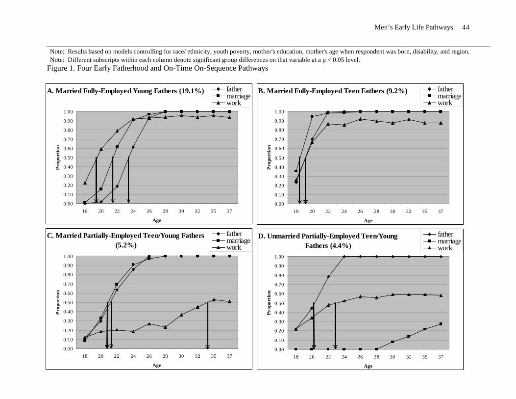
Men’s Early Life Pathways 44
Note: Results based on models controlling for race/ ethnicity, youth poverty, mother's education, mother's age when respondent was born, disability, and region. Note: Different subscripts within each column denote significant group differences on that variable at a p < 0.05 level.
Figure 1. Four Early Fatherhood and On-Time On-Sequence Pathways
A. Married Fully-Employed Young Fathers (19.1%)
0.00
0.10
0.20
0.30
0.40
0.50
0.60
0.70
0.80
0.90
1.00
18 20 22 24 26 28 30 32 35 37
Age
Prop
ortio
n
fathermarriagework
B. Married Fully-Employed Teen Fathers (9.2%)
0.00
0.10
0.20
0.30
0.40
0.50
0.60
0.70
0.80
0.90
1.00
18 20 22 24 26 28 30 32 35 37
Age
Prop
ortio
n
fathermarriagework
C. Married Partially-Employed Teen/Young Fathers (5.2%)
0.00
0.10
0.20
0.30
0.40
0.50
0.60
0.70
0.80
0.90
1.00
18 20 22 24 26 28 30 32 35 37
Age
Prop
ortio
n
fathermarriagework
D. Unmarried Partially-Employed Teen/Young Fathers (4.4%)
0.00
0.10
0.20
0.30
0.40
0.50
0.60
0.70
0.80
0.90
1.00
18 20 22 24 26 28 30 32 35 37
Age
Prop
ortio
n
fathermarriagework
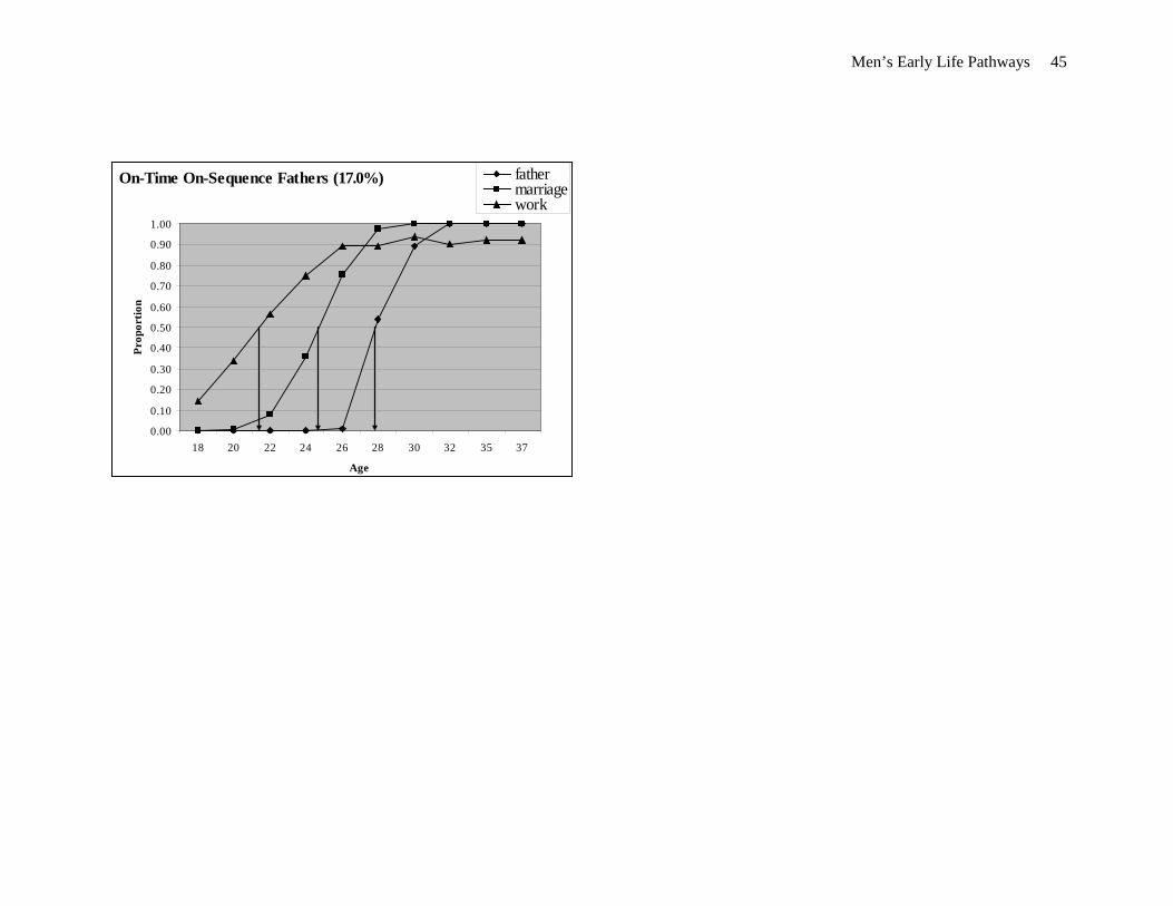
Men’s Early Life Pathways 45
On-Time On-Sequence Fathers (17.0%)
0.00
0.10
0.20
0.30
0.40
0.50
0.60
0.70
0.80
0.90
1.00
18 20 22 24 26 28 30 32 35 37
Age
Prop
ortio
n
fathermarriagework