Passive and Active Currency Portfolio Optimisation

1

Passive and Active Currency Portfolio

Optimisation

by

Fei Zuo

Submitted by Fei Zuo, to the University of Exeter as a thesis for the

degree of Doctor of Philosophy in Finance, February 2016.

This thesis is available for Library use on the understanding that it is

copyright material and that no quotation from this thesis may be

published without proper acknowledgement.

I certify that all material in this thesis which is not my own work has

been identified and that no material has previously been submitted and

approved for the award of a degree by this or any other University

Signature: …………………………………………………………..

3

To my parents and my wife

5

Acknowledgement

I would like to give my deepest gratitude first and foremost to Professor Richard Harris,

my first supervisor, for his constant encouragement and guidance. He has guided me

through all stages of the writing of this thesis. Without his consistent and illuminating

instruction, this thesis could not have reached its present form.

I would also like to acknowledge Dr Jian Shen, my second supervisor, for her help with

instructions and data collection. She instructed me for all fours years of my PhD study,

and provided a lot of suggestions. She also facilitated access to DataStream. Without

her help, this thesis could not have been successfully completed.

This thesis is dedicated to my parents and my wife. I would like to take this opportunity

to say thank you to my beloved parents for their consideration and great confidence in

me throughout all these years. I also would like to say thank you to my loving wife for

taking care of my daughter and doing household duties. Without your support and

encouragement, it would have been difficult to come to the UK and finish my Masters

and PhD degrees at The University of Exeter.

Special thanks go to Professor Pengguo Wang for giving me an opportunity to work

with him about exam materials on ELE. I really enjoyed this work.

I gratefully acknowledge the graduate teaching assistantship opportunity availed to me

by the University Of Exeter School Of Business. This gave me sufficient funding and

valuable teaching experience.

7

Abstract

This thesis examines the performance of currency-only portfolios with different

strategies, in out-of-sample analysis.

I first examine a number of passive portfolio strategies into currency market in out-of-

sample analysis. The strategies I applied in this chapter include sample-based mean-

variance portfolio and its extension, minimum variance portfolio, and equally-weighted

risk contribution model. Moreover, I consider GDP portfolio and Trade portfolio as

market value portfolio for currency market. With naïve portfolio, there are 12 different

asset allocation models. In my out-of-sample analysis, naïve portfolio performs

reasonably well among all 12 portfolios, and transaction cost does not seriously affect

the results prior to transaction cost analysis. The results are robust across different

estimation windows and perspectives of investors from different countries.

Next, more portfolio strategies are examined to compare with naïve portfolio in

currency market. The first portfolio strategy called ‘optimal constrained portfolio’ in

this chapter is derived from the idea of maximising the quadratic utility function. In

addition, the timing strategies, a set of simple active portfolio strategies, are also

considered. In my out-of-sample analysis with rolling sample approach, naïve portfolio

can be beaten by all the strategies discussed in this chapter.

In chapter six, the characteristics of currency are exploited to construct a currency only

portfolio. Firstly, the pre-sample test proves that the characteristics, both fundamental

and financial, are relevant to the portfolio construction. I then examine the performance

of parametric portfolio policies. The results show that while fundamental characteristics

can bring investor benefits of active portfolio management, financial characteristics

8

cannot. Moreover, I find the relationship between characteristics of currency and

weights of optimal portfolio.

The overall results show that currencies can be thought of as an asset in their own right

to construct optimal portfolios, which have better performance than naïve portfolio, if

suitable strategies are used. In addition, ‘lesser’ currencies, indeed, bring significant

benefits to the investors.

9

Table of Contents

List of Tables and Figures ........................................................................................................ 13

Abbreviation .............................................................................................................................. 15

Chapter One .............................................................................................................................. 17

Introduction ............................................................................................................................... 17

1.1 Background ................................................................................................................ 17

1.2 Motivation .................................................................................................................. 19

1.3 Contribution and Empirical Results........................................................................ 21

1.4 Organisation of This Thesis ...................................................................................... 24

Chapter Two .............................................................................................................................. 27

Literature Review ...................................................................................................................... 27

2.1 Portfolio Strategies .................................................................................................... 29

2.1.1 Markowitz Model and Sample-based Mean-Variance Portfolio .................. 29

2.1.2 Error in Estimation and Extension Models .................................................... 32

2.1.3 Combination Portfolio ...................................................................................... 35

2.1.4 Equally-weighted Risk Contribution Portfolio ............................................... 36

2.1.5 Optimal Constrained Portfolio......................................................................... 37

2.1.6 Timing Strategies ............................................................................................... 38

2.1.7 Parametric Portfolio Policy .............................................................................. 39

2.2 Characteristics of Currency ..................................................................................... 41

2.2.1 Financial Characteristics .................................................................................. 42

2.2.2 Fundamental Characteristics ........................................................................... 43

2.3 Performance Evaluation Methods ........................................................................... 45

2.3.1 Traditional Performance Measures ................................................................. 45

2.3.2 Comparison of Sharpe Ratios .......................................................................... 47

2.3.3 Risk Measure based on Drawdown ................................................................. 48

2.3.4 Risk Measure based on Quantiles .................................................................... 49

2.4 Conclusion .................................................................................................................. 51

Chapter Three ........................................................................................................................... 53

Data............................................................................................................................................. 53

3.1 Currency Return ....................................................................................................... 54

3.1.1 Method of Calculation ...................................................................................... 54

3.1.2 Spot Rate ............................................................................................................ 55

3.1.3 Forward Rate ..................................................................................................... 55

3.1.4 Risk Free Rate ................................................................................................... 60

10

3.1.5 GDP and Trade .................................................................................................. 62

3.2 Summary Statistics .................................................................................................... 62

3.2.1 Currency Return ............................................................................................... 63

3.2.2 Risk Free Rate ................................................................................................... 65

3.2.3 GDP and Trade .................................................................................................. 65

3.3 Turnover and Adjustments for Transaction Cost .................................................. 67

3.4 Conclusion .................................................................................................................. 68

Chapter Four ............................................................................................................................. 69

Currency Portfolio Management: Passive Portfolios vs Naïve Portfolio ............................. 69

4.1 Introduction ............................................................................................................... 69

4.2 Empirical Framework ............................................................................................... 74

4.2.1 Portfolio Construction Models ......................................................................... 75

4.2.2 Performance Evaluation Method ..................................................................... 79

4.2.3 Estimation Method ............................................................................................ 81

4.3 Empirical Results ...................................................................................................... 82

4.3.1 Main Results ...................................................................................................... 82

4.3.2 Results after Transaction Cost ......................................................................... 86

4.3.3 Robustness for Different Lengths of Estimation Windows ........................... 89

4.3.4 Robustness for Investor Perspectives from Different Countries................... 96

4.4 Conclusions .............................................................................................................. 105

Chapter Five ............................................................................................................................ 107

Currency Portfolio Management: Timing Strategies .......................................................... 107

5.1 Introduction ............................................................................................................. 107

5.2 Portfolio Strategies .................................................................................................. 112

5.2.1 Optimal Constrained Portfolio....................................................................... 112

5.2.2 Timing Strategies ............................................................................................. 114

5.3 Monte Carlo Experiment ........................................................................................ 116

5.3.1 The Experiment ............................................................................................... 117

5.3.2 Results of the Experiment ............................................................................... 118

5.4 Empirical Results .................................................................................................... 121

5.4.1 Preparation before Analysis ........................................................................... 121

5.4.2 Main Results .................................................................................................... 124

5.4.3 Robustness Check for Different Lengths of Estimation Windows ............. 131

5.4.4 Robustness Check for Investor Perspectives from Different Countries ..... 140

5.5 Conclusion ................................................................................................................ 149

Chapter Six .............................................................................................................................. 153

Currency Portfolio Management: Exploiting Characteristics ............................................ 153

11

6.1 Introduction ............................................................................................................. 153

6.2 Portfolio Strategy .................................................................................................... 159

6.2.1 Basic Approach ................................................................................................ 159

6.2.2 Method of Estimating ................................................................................. 161

6.2.3 Transaction Cost ............................................................................................. 162

6.3 Data ........................................................................................................................... 163

6.3.1 Financial Characteristics ................................................................................ 163

6.3.2 Fundamental Characteristics ......................................................................... 164

6.4 Empirical Analysis .................................................................................................. 167

6.4.1 Pre-sample Test ............................................................................................... 167

6.4.2 Out-of-sample Analysis ................................................................................... 172

6.4.3 Robustness Check ............................................................................................ 183

6.4.4 Investigation of Coefficients for Out-of-sample Analysis ............................ 193

6.5 Conclusion ................................................................................................................ 196

Chapter Seven .......................................................................................................................... 199

Conclusion and Future Research ........................................................................................... 199

7.1 Conclusion ................................................................................................................ 199

7.2 Limitation ................................................................................................................. 202

7.3 Future Research ...................................................................................................... 203

References ................................................................................................................................ 207

13

List of Tables and Figures

Chapter two

Figure 2.1 Mean-Variance Analysis

Chapter three

Table 3.1 List of currencies with absent forward rate

Table 3.2 Weights and names of risk free rate of six euro countries

Table 3.3 Statistics of 29 currencies returns

Figure 3.1 Statistics of percentage of difference between calculated FWD and quoted

FWD over quoted FWD

Figure 3.2 Comparison of calculated FWD with quoted FWD

Figure 3.3 Average weight of each currency for GDP and Trade portfolios

Chapter four

Table 4.1 The evaluation results for portfolios with G10 currencies

Table 4.2 The evaluation results for portfolios with all currencies

Table 4.3 Comparison of results from before and after transaction cost for G10

currencies

Table 4. 4 Comparison of results from before and after transaction cost for ALL

currencies Table 4.5 Robustness results for 1 year estimation window

Table 4.6 Robustness results for 3 year estimation window


Table 4.8 Comparing Sharpe ratio for same evaluation period with different lengths of

estimation windows

Table 4.9 Robustness results for perspective of UK investors

Table 4. 10 Robustness results for perspective of Japanese investors

Table 4.11 Robustness results for perspective of Euro zone investors

Chapter five

Table 5.1 Evidence from Monte Carlo Simulation

Table 5.2 Performance of the portfolios for G10 currencies

Table 5.3 Performance of the portfolios for all currencies


Table 5.5 Robustness results for 3 years estimation window



Table 5.8 Robustness results for perspective of JP investors

Table 5.9 Robustness results for perspective of EZ investors

14

Chapter six

Table 6.1 performance of each strategy for in sample analysis

Table 6.2 coefficients of variables and their p-value from a bootstrap process

Table 6.3 Performance of portfolios related to naïve portfolio

Table 6.4 Performance of portfolios related to volatility timing portfolio

Table 6.5 Performance of portfolios related to minimum variance



Table 6.8 Robustness results for perspective of Euro investors

Table 6.9 The average of coefficients for all out-of-sample analyses

15

Abbreviation

Forex Foreign Exchange Market

OC Optimal Constrained portfolio

PPP Parametric Portfolio Policy

CRRA Constant Relative Risk Aversion

BEER Behavioural Equilibrium Exchange Rate model

VaR Value at Risk

CVaR Conditional Value at Risk

MDD Maximum Drawdown

GDP Gross Domestic Product

CEQ Certainty-Equivalent

ERC Equally-weighted Risk Contribution portfolio

VT Volatility Timing portfolio

RR Reward-to-Risk portfolio

EWMA Exponentially Weighted Moving Average

SMA Simple Moving Average

GMVP Global Minimum Variance Portfolio

CML Capital Market Line

HICP Harmonised Index of Consumer Prices

RIR Real Interest rates

TNT Traded to Non-Traded Goods (Productivity)

TOT Term of Trade

GC Government Consumption

CPI Consumer Price Index

17

Chapter One

Introduction

1.1 Background

Markowitz portfolio theory, widely considered as a cornerstone of modern portfolio

theory, was derived by Markowitz in 1952. He assumes that investors are only

concerned with the mean and variance of a portfolio’s return. Due to preference of

higher returns with the same risk, investors will choose tangency portfolio. The idea of

this strategy seems right. However, due to moments estimated by sample analogues, the

implementation of this model performs poorly out of the sample (Michaud, 1989). A

number of studies have focused on this topic leading to the development of this model

with some adjustments. Other studies also tried to create alternative methods for

constructing portfolios that could beat the market. All these models have been

empirically applied to stock and/or bond markets for efficiency testing.

Investors were starting to realise that investment diversification cannot only be done in

their own country, but also around the world, with the latter resulting in additional

benefits. Grubel (1968) describes and quantifies the benefits derived from international

diversification, and concludes this diversification as a new source of gains. In their

deliberations, Levy and Sarnat (1970) not only further support the Grubel’s findings,

but also suggest investing in both developed and developing countries, because less

correlated returns can reduce overall portfolio variance as well as risk. In the two

decades prior to 1970, due to relatively stable exchange rates, international investments

did not need to consider foreign currency holdings for the international diversification.

18

However, due to collapse of the Bretton Woods system, the currency exchange rates are

able to float freely, which can be considered as a source of financial risk. Eun and

Resnick (1988) argue that the studies from Grubel (1968) and Levy and Sarnat (1970)

are overstating the actual gains made from international diversification, because of the

factor that parameter uncertainty is not accounted. The risks inherent to foreign

exchange rates can eliminate or substantially reduce the profit made on an international

portfolio.

International investment in bonds and equities, therefore, introduces an additional

source of risk, which is due to floating-free exchange rates. A number of studies have

addressed this risk by hedging strategies that sell the expected foreign currency returns

at forward rate. For example, Black (1989) introduced the concept of ‘universal hedging’

which suggests that investors should always hedge their foreign assets equally for all

countries but never 100%. The effectiveness of hedging strategy is dependent upon an

investor’s ability to estimate future returns. Glen and Jorion (1993), Larsen Jr and

Resnick (2000) and Topaloglou et al. (2008) had similar findings supporting the fact

that hedged portfolios dominate non-hedged portfolios. More research on hedging

strategy include Schmittmann (2010), who studied the impact of hedging the currency

risk from the perspectives of different national investors over period including the last

financial crisis period, and Fonseca et al. (2011), who extend the robust model to

include currency option as a hedging instrument.

However, currencies are increasingly thought of as an asset in their own right. Levy and

Sarnat (1978) report achievement of significant gains from holding foreign currencies

from a US investor perspective. They firstly calculate mean and standard deviations of

monthly return on the holding of foreign currencies from 1959 to 1973. In the periods

prior to 1970, the mean returns were either negligible or negative. However, after 1970,

19

the mean returns for most of the currencies are significantly positive, and fluctuations

were enlarged. And then, they optimised that most currencies provide a higher rate of

return than the Standard and Poor’s Common Stock Index did. They also analysed and

confirmed the gains from diversification for only currencies portfolios and portfolios of

foreign currency and country’s stock index. The basic concept of their report is to treat

foreign currencies as an investment asset not a hedge tool. According to BIS Triennial

Survey (2007), there are $3.2 trillion being exchanged on a daily basis ($4 trillion in

2010), which indicates that the Foreign Exchange Market (Forex) could be considered

as the biggest single market in the world. So, more and more currencies could be

considered as another type of asset, which I could invest in and find speculating

opportunity like I have done in the stock or bond market.

1.2 Motivation

The existing research on portfolio optimisation for currencies is not extensive. Some

studies try to use active portfolio management to find out the speculating opportunity in

Forex. Dunis et al. (2011) uses cointegration introduced by Engle and Granger (1987) to

diversify a currency trading portfolio, in order to find the benefit, if any. In general,

cointegration-based optimization strategies add value, but, as all optimization

techniques, they should be used cautiously. Schmittmann (2010) applies currency carry

trading strategy with MGARCH-based carry-to-risk portfolio optimization to construct

a portfolio containing Brazilian real and Mexican peso. They found that this dynamic

approach leads to a significant surplus profit in times of either very low or very high

volatility. Cao et al. (2009) introduce a novel portfolio optimization method for foreign

currency investment. They use support vector machines and neural network and moving

average to predict exchange rates and build a portfolio by adopting multi-objective

portfolio optimization technique by maximising the return and minimizing the risk. The

20

results show superior return performance of optimal portfolio compared with single

currency investment. However, the studies mentioned above regarding currency

portfolio optimisation are not systematic, and include only a small number of currencies.

Moreover, very few studies have considered passive portfolio investment among

currencies. A most relevant research about passive currency-only portfolios is written

by Levy and Sarnat (1978). They simply applied basic idea of modern portfolio theory

by sample mean and standard deviation to construct a set of efficient portfolios. They

analysed Tobin’s separation theorem and illustrated the statistics and composition of

tangency portfolio. Furthermore, they conclude that an investor will not hold domestic

cash in his portfolio, but blend the optimal portfolio with riskless bonds. However, they

did not compare results to other portfolios constructed using different methodologies.

Recently, a number of robust models and alternative methods were created to develop

the performance of Markowitz model. But, few researches applied these methods into

construction of currency-only portfolio.

Based on the considerations above, my thesis provides a comprehensive analysis of both

passive and active portfolio management models in currency portfolio optimization. As

I have already indicated, researchers always study currencies as a hedge tool to reduce

the risk, at cost, on international investments, but are limited to find out optimal

solutions for the gain from exchange rate fluctuations by portfolio optimization strategy.

So, the gap in the literature is to analyse the performance of optimal portfolios for

currency only portfolio. This study aims at filling this gap. Filling this gap is important

to investors who desire to take a position on foreign currencies, due to the nature and

magnitude of their economic activities, such as central bank, international investment

trusts, and large multinational corporations.

21

1.3 Contribution and Empirical Results

The first contribution of the thesis is the systematic examination of the out-of-sample

performance of currency only portfolios. As discussed before, the literature about the

performance of currency only portfolio is limited, and methods for evaluating are

simple, and the number of currencies is small. So, in my thesis, the evaluation methods I

use are comprehensive, including not only trade-off between return and risk but also

downside risks. A total of 29 currencies are included in this thesis, which almost include

all free-floating currencies without high correlation. So, I call portfolio including 29

currencies as all currencies portfolio. I consider naïve portfolio as benchmark to

compare other optimal portfolios. Moreover, I use three chapters to investigate the

performance of currency portfolios with various strategies from passive to active. In the

next several paragraphs, I will show what strategies I use and results of their

performance.

In Chapter four, I examine a number of passive portfolio strategies into currency market

in an out-of-sample analysis. The strategies I applied in this chapter include sample-

based mean-variance portfolio, its extension, minimum variance portfolio, and equally-

weighted risk contribution model. Moreover, I consider GDP portfolio and Trade

portfolio as market value portfolio for the currency market. With naïve portfolio, there

are 12 different asset allocation models. In the out-of-sample analysis, the results show

that the sample-based mean-variance portfolio works very badly with low Sharpe ratio

and horrible downside risk, because of an estimation error. Moreover, the minimum

variance portfolios, with and without short-sale constraint, has the best performance and

exposure to the lowest downside risk. The naïve portfolio and equally-weighted risk

contribution portfolio also perform reasonable well. I also take account of transaction

22

cost, and compare the results before and after transaction cost. But, transaction cost does

not seriously affect the rankings from before transaction cost analysis.

In Chapter five, more portfolio strategies are examined to compare with naïve portfolio

in currency market. The first portfolio strategy is called as optimal constrained (OC)

portfolio, which is based on the mean-variance portfolio and target portfolio return to be

the conditional mean of naïve portfolio. In addition, the timing strategies, a set of simple

active portfolio strategies, are also considered. For my analysis about currency only

portfolio, optimal constrained and volatility timing portfolio consistently outperform

naïve portfolio in all terms of evaluation I used. The transaction cost does not change

the conclusion, although it reduces the performance of portfolios. In addition, I find that

exponentially weighted moving average is more efficient to estimate conditional

expected moments than simple moving average to reduce estimation error.

In chapter six, I examine an alternative active portfolio strategy, called parametric

portfolio policy (PPP). Its weights are calculated as linear function of characteristics of

currency plus benchmark weights. The results of my out-of-sample analysis about

currency only portfolio display that fundamental characteristics can give CRRA

investor benefits of active portfolio management, but financial characteristics cannot.

But, considering both classes of characteristics together worsens the performance of

PPP portfolio. If the investors are safety-first rather than CRRA investor, the PPP

portfolio still is their choice in a way. Although a high level of turnover of PPP

portfolios, the transaction cost does not change my conclusions.

The second contribution of the thesis is the examination of international diversification

benefit from investing in currencies of developing countries. The fact about more gains

from investing globally has been proved again and again by the literature, since the

studies by Grubel (1968) and Levy and Sarnat (1970). After free-floating, some studies

23

(e.g. Black, 1989; Larsen Jr and Resnick, 2000; Fonseca et al., 2011) provide empirical

evidence that international investment benefit can still be gained by hedging floating

risk using currency derivatives. But, there are few studies (only Dunis et al., 2011) that

focus on the benefit of global investment for currency. Once I invest in Forex, the

currencies bought are already from different countries. Therefore, globally investing or

international investment, in this thesis, means that investors invest in both developed

and developing countries’ currencies. Due to the fact that currencies of developing

countries are less traded compared to currencies of developed countries; the developing

countries’ currencies are often referred to as ‘lesser’ currency in the rest of this thesis. I

firstly examine the performance of portfolios which only contains G10 currencies. And

then, I compare it with the performance of portfolios, which use same strategies but

contain G10 currencies and ‘lesser’ currencies. This is the first study to examine benefit

from investing in ‘lesser’ currencies, using vast portfolio strategies. This method is

different from the study by Dunis et al. (2011), which added ‘lesser’ currencies one by

one. The results from chapter four and chapter five show that the performance of all

currencies portfolio is significantly better than that of G10 currencies portfolio. So, I

can conclude that adding ‘lesser’ currencies can help investors gain the huge benefit

from diversification.

The third contribution of the thesis is to provide a guide to construct currencies portfolio

by using their fundamental characteristics, and examine the performance of this strategy

in out-of-sample. The basic idea I used in this thesis is from a study by Brandt et al.

(2009). In equity market, they adjust portfolio weights from market weights by

characteristic of stocks, and name this strategy as parametric portfolio strategy. But,

there are challenges when this strategy is applied into currency market. Firstly, currency

has its own characteristics, which are not the same as stocks. Although Barroso and

Santa-Clara (2011) examine the performance of currency only portfolio constructed by

24

parametric portfolio policy, the characteristics they only focus on are financial variables,

which are calculated by the historical performance of currency. But, fundamental

variables, the factors that determine currency exchange rate, can also be considered to

construct portfolio weights. Therefore, in chapter six, the fundamental characteristics of

currency also are investigated to construct currency only portfolio. The results from the

pre-sample test prove that the characteristics, both fundamental and financial, are

relevant to the portfolio construction. Secondly, unlike equity market, there is no market

portfolio with value-weighted average. So, I consider two portfolio weights as

benchmark weights. One is naïve weights, and another one is volatility timing portfolio

weights. The results from out-of-sample analysis of chapter six confirm that the choice

of benchmark weights is not important to the investor. In addition, I find that the PPP

portfolios allocate considerably more wealth to currencies with small interest rate

spread, large real interest rates differential, strong productivity differential, and small

term of trade differential.

1.4 Organisation of This Thesis

The remainder of this thesis is organised as follows. In Chapter two, a critical analysis

of existing literature on portfolio management is undertaken. This is help in justifying

the research objectives and questions. In order to give readers a complete picture, the

evaluation methods are also mentioned.

In chapter three, I describe the data used in this thesis. The description includes data

collection and the method of currency return calculation. Moreover, I discuss the

statistics of currency return and relevant data. In addition, the method of taking account

of transaction cost is introduced.

25

In Chapter four, I test 12 different optimal passive portfolios in currency market. The

out-of-sample analysis confirms that the naïve portfolio performs very well, which is

consistent with existing literature for equity market. But, minimum variance portfolio

has the best performance. The results indicate a support of good performance of naïve

portfolio.

In Chapter five, I analyse several active portfolio strategies, which have been proved to

have better performance than naïve portfolio for equity market by existing literature.

The main results show the same conclusion. But, for the robustness check, the results

are inconclusive. Both chapters have two datasets---only G10 currencies and G10

currencies with ‘lesser’ currencies. The comparison shows significant international

diversification benefit.

In Chapter six, I investigate characteristics of currency to construct optimal portfolio,

and test the performance of this portfolio. The results of pre-sample test show that both

financial and fundamental characteristics are relevant to the portfolio construction. And,

the results of out-of-sample analysis show that PPP portfolio with fundamental

characteristics has the best performance, which can beat naïve portfolio.

The last chapter concludes the results of the thesis and gives directions for future

research. This chapter brings together the work of the dissertation by showing how the

initial research plan has been addressed in such a way that conclusions may be formed

from the evidence of the dissertation. This will also outline the extent to which each of

the aims and objectives has been met. Research questions are also reintroduced in order

to give a clear understanding to the reader.

27

Chapter Two

Literature Review

In this chapter, I firstly review the literature related to portfolio management, which has

been considerably advanced since seminal works of Markowitz (1952). Because of the

factor that the moments of return are estimated with significant errors, an extensive

literature review makes significant effort to handle this estimation error in the purpose

of improving performance of portfolio. The popular approach applied in a vast literature

is Bayesian approach to estimation error, including purely statistical approach relying

on diffuse-priors (Barry, 1974; Brown, 1979), idea of shrinkage estimation (James and

Stein, 1961; Jorion, 1986), and recent model depend on the asset-pricing model (Pástor

and Stambaugh, 2000; Wang, 2005). Another equally rich set of approach is related to

non-Bayesian approach to estimation errors. This includes rules about robust portfolio

with uncertainty of parameters and model (Garlappi et al., 2007), Three-fund

combination portfolio (Kan and Zhou, 2007; DeMiguel et al., 2007), Optimal constrain

portfolio to target conditional expected portfolio return to naïve portfolio return (Kirby

and Ostdiek, 2010), and the simplest way to put short-sale constrains into portfolios

construction (Frost and Savarino, 1988; Chopra, 1993; Jagannathan and Ma, 2003). In

addition, there are alternative strategies, beyond to Markowitz‘s model (1952), also

developed and tested in recent literature, such as a strategy to weight risk contribution

equally (Neukirch, 2008b; Maillard et al., 2008), a rule focusing on changes in volatility

through time (Fleming et al., 2003; Kirby and Ostdiek, 2010), a novel approach to

directly construct portfolio based on only characteristics of assets (Brandt et al., 2009),

and the simple non-optimised naïve portfolio (DeMiguel et al., 2007).

28

In the second part of this section, a critical analysis of literature pertaining to the

characteristics of currency is undertaken. The frequent trading strategy in currency

market is carry trade, which buys currency with high interest rate and sells currency

with low interest rate (Bilson, 1981; Fama, 1984; Burnside et al., 2008). Besides carry

trade, other two currency trading strategies, currency moment and value, are also

profitable (Menkhoff et al., 2012b; Okunev and White, 2003; Burnside et al., 2011;

Asness et al., 2013). Barroso and Santa-Clara (2011) conclude this three currency

trading strategies as financial characteristics of currency. In addition to financial

characteristics, the approach of behavioural equilibrium exchange rate (BEER), which

extended from relative purchasing power parity, determine exchange rate by some

economic factors (Clark and MacDonald, 1999). These economic factors can be

considered as fundamental characteristics of currency, and are employed in the literature

by different sets (Komárek et al., 2005; Lane and Milesi-Ferretti, 2001, MacDonald and

Dias, 2007; Cheung et al., 2005).

The final part of this section is to review the method of evaluating performance of

portfolio in the literature. Sharpe (1994) defines a famous and standard performance

measure as Sharpe ratio, which trade-off between return and standard deviation of

return. There are also other measures considered in the literature to trade-off return and

risk. But, Caporin and Lisi (2009) conclude that the results from others are similar to it

from Sharpe ratio. Recently, there alternative approaches to measure risk have been

developed. One is related to the Drawdown, which represent the maximum loss at time t

from time 0 (Biglova et al., 2004; Ortobelli et al., 2005; Rachev et al., 2008). Another

risk measure is based on the quantiles of series of returns. The simple version is always

called as value at risk (Beder, 1995). Due to significant loss in global financial crisis by

use of VaR (Kidd, 2012), investors have adopted a conditional value at risk, which was

first proposed by Embrechts et al. (1999) and measure tail risk.

29

2.1 Portfolio Strategies

2.1.1 Markowitz Model and Sample-based Mean-Variance Portfolio

In financial markets, the risk has been dealt with a long history. When shares of the East

India Company began trading in Amsterdam in 1602, the first stock market was built

(Perold, 2004). But, the trade-off between risk and return is formally stated by

Morgenstern and Von Neumann (1944), who also develop the utility function of this

trade-off.

Markowitz (1952, 1959) firstly considers variance as a measure of risk formally, and

then tries to construct portfolios by the risk-return trade-off. He assumes that investors

are risk averse and the only matter they care about is the mean and variance of return of

portfolios for the holding period. According to these assumptions, investors will choose

the portfolios which have minimum variance for a given expected return or maximum

expected return for a given variance. Figure 2.1 demonstrates all possible portfolios the

investors faced for mean and variance analysis. When there are only risky assets taken

into account, the efficient frontier is curve above point b, which represents global

minimum variance portfolio (GMVP). But, if considering about risk free asset, the

efficient frontier is now a straight line throughfR and M, which is the tangency

portfolio. This straight line is also referred to as Capital market line by Sharpe (1964)

and Lintner (1965), and the tangent point M is called market portfolio as well.

30

Figure 2.1 Mean-Variance Analysis

The figure plots the flexible and efficient set of mean and variance analysis of Markowitz, and Capital market line of

Sharpe (1964) and Linter (1965). E(R) is the expected return and σ(R) is the standard deviation of returns. When

there are only risky assets, point b represents the global minimum variance portfolio (GMVP). The curve abc and the

area within belong to flexible set. But, the only curve above point b is efficient, called efficient frontier. When there

is a risk free asset, M represents risk free rate and Market portfolio, which is the tangent point from risk free ratefR .

the straight line from fR and M is the new efficient frontier.

CML

M

σ(R)

c

a

b

E(R)

31

A vast amount of literature, e.g. DeMiguel et al. (2007), Kolusheva (2008), Brandt

(2009) Kirby and Ostdiek (2010), derives a formula of tangency portfolios weights from

mean-variance utility function. According to Markowitz model above, investors choose

the optimal combination lies on CML. This combination has a vector of risky asset

weights x and )1( ' xN of risk free asset, where N is an N-dimensional vector of ones

and N is number of risky assets. The exact position of investor is determined by his

tolerance for risk. Therefore, they use to denote relative risk aversion of investor, and

select x , N*1 vector, by maximise expected utility function:

max𝑥 𝑥′ 𝜇 −𝛾

2𝑥′Σ𝑥 (2.1)

In which is an N-dimensional vector of the expected excess returns over risk free rate,

Σ is N*N matrix of variance and covariance of expected excess returns. The solution of

the problem is:

𝑥∗ =1

𝛾Σ−1𝜇 (2.2)

The vector of relative weights in risky only asset portfolio (tangency portfolio) is:

𝑤𝑇𝑃 =𝑥∗

|𝟏𝑁′ 𝑥∗|

(2.3)

After taking equation 2.2 into equation 2.3, they have tangency portfolio weights:

𝑤𝑇𝑃 =Σ−1𝜇

𝟏𝑁′ Σ−1𝜇

(2.4)

In order to construct portfolio, investor has to estimate the expected excess return and

variance-covarianceΣ . The simplest way used by Markowitz (1952, 1959) is ‘plug-in’

approach, which is to estimate and by using their historical sample analogues

(sample mean ,N*1 vector, and sample variance-covariance matrix Σ , N*N matrix).

32

This strategy is referred as ‘sample-based mean-variance portfolio’ or ‘Plug-in estimates’

mean-variance portfolio, and the vector of its weights is calculated as follow:

𝑤𝑆𝐵 =Σ−1��

𝟏𝑁′ Σ−1��

(2.5)

The problem of this sample based strategy is ignorance of estimation error. In the next

section, the literature related to this error will be reviewed.

2.1.2 Error in Estimation and Extension Models

The fact that error in estimation is reason of poor performance of sample-based mean-

variance portfolio in out-of-sample is well documented in the literature. As noted in a

number of studies, Kolusheva (2008) concludes that the sensitivity to small change in

inputs data is the root of failure of sample-based mean-variance portfolio in out-of-

sample analysis. Chopra (1993) finds that mean-variance portfolios can be vastly

different, even estimates are slightly changed. This analysis has also been done by Best

and Grauer (1991). Dickinson (1974) recognizes the impact of parameter uncertainty

on optimal portfolio selection, and point out that this approach is seriously hampered by

estimation error, according to practical application of portfolio analysis. Jobson and

Korkie (1980) clearly illustrate the reason of imprecision of plug-in estimates, according

to a simple example, which only considers one risky asset in the universe. They use a

typical stock with =8% and =20% to calculate the standard error of the plug-in

estimator, which is large relative to the magnitude of true value. Michaud (1989) points

out that the estimation error in sample-based parameters leads to extreme weights that

fluctuate substantially over time and perform poorly out of sample. This has motivated

that sample-based mean-variance optimizers are ‘error maximisers’, which is

widespread view in academic literature.

33

Therefore, the vast literature made efforts to reduce estimation errors. A prominent role

to solve estimation error is acted by the Bayesian approach. Under this approach, and

Σ are estimated by using predictive distribution of asset returns. In order to obtain this

distribution, the conditional likelihood is integrated over and Σ with respect to a

certain subjective prior. The studies implement this approach in different ways. Firstly,

Stein (1956) and James and Stein (1961) firstly pioneer an application of the idea of

shrinkage estimation. In order to mitigate the error for estimating expected returns, they

shrink the sample mean of individual asset returns toward ‘grand’ mean across all assets.

Jorion (1986) not only shrink the estimate of mean by taking grand mean to be mean of

minimum-variance portfolio, but also use traditional Bayesian-estimation methods to

account for estimation error in the covariance matrix. Because of combining both a

shrinkage approach and a traditional Bayesian estimation, the portfolio constructed

under this approach is called as ‘Bayes-stein’ portfolio, which was applied into practice

by DeMiguel et al. (2007). Secondly, Barry (1974) and Brown (1979) provide a

correction based on a diffuse prior. In their approach, the estimation risk is reduced by

inflating the covariance matrix. But, because the estimator of expected returns is still a

sample mean, the effect of this correction is negligible. Finally, Pástor (2000) and

Pástor and Stambaugh (2000) recently proposed the Bayesian ‘Data-and Model’

approach, which depends on a particular asset-pricing model the investor believes in.

Under this approach, the shrinkage target and factor are determined by the investor’s

belief related to an asset-pricing model and its validity. Then, according to Bayesian

‘Data-and Model’ approach, Wang (2005) provides a method to obtain estimators for

the mean and variance-covariance matrix of asset return. DeMiguel et al. (2007)

implements it using three different asset-pricing models: the CAPM, the three-factor

model (Fama and French, 1993) and four-factor model (Carhart, 1997).

34

In addition to Bayesian approach, the set of non-Bayesian approaches are also equally

rich in the literature for reducing estimation error. Merton (1980) points out that the

expected returns are very hard to estimate from historical returns. He concludes that

errors in the estimates of expected returns are larger than those in the estimate of

variance-covariance matrix. For this reason, the global minimum variance portfolio,

which does not incorporate information on the expected return, is influenced by the

recent vast literature (Best and Grauer, 1992; Chan et al., 1999; Ledoit and Wolf,

2003a). This minimum variance portfolio can be thought of as a special case of mean-

variance portfolio, when all risky assets in the universe have the same expected return.

In this special case, if the variance-covariance matrix is a scale of the identity matrix as

well, the weights of mean-variance portfolio will be the same for all risky assets. This

equalled weighted portfolio, referred to as naïve portfolio, completely ignores the data

without any optimization and estimation. But, DeMiguel et al. (2007) provide strong

empirical evidence that many optimal portfolios cannot beat the naïve portfolio. They

analyse the out-of-sample performance of naïve portfolio against numerous other

optimization strategies. In the real world, Benartzi and Thaler (2001) investigate many

participants in defined contribution plan, and show naïve portfolio is a popular strategy.

Windcliff and Boyle (2004) argue that naïve portfolio is not naïve as it appears, and

shows that it can provide protection against very bad outcomes. In order to help reduce

estimation error, there is another simple method, which only allows non-negative

weights (short-sale constraints) in optimizing process (Frost and Savarino, 1988;

Chopra, 1993). They also explain that the short-sale constraints are similar to shrinkage

of expected return towards zero. In addition, a wide range of literature has made an

effort to develop new approaches to deal with estimation risk remains with respect to

variance-covariance matrix, such as, imposing a strong structure by using constant

correlation (Elton and Gruber, 1976), applying single index approach which determines

35

a covariance based on the level of relationship (Sharpe, 1963). An approach to estimate

covariance matrix by using means of shrinkage estimators (Ledoit and Wolf, 2003a;

Kempf and Memmel, 2003), and a new one-step approach which directly estimates

optimal portfolio weights rather than estimate return distribution parameters first and

then optimise portfolio weights (Kempf and Memmel, 2003). However, Jagannathan

and Ma (2003) prove that for the minimum-variance portfolio, a short-sale constraint

imposing have the same effect as shrinking the element of the covariance matrix.

2.1.3 Combination Portfolio

In recent years, there has emerged an alternative idea to construct portfolio by

combining other portfolios. This idea tries to apply shrinkage to portfolio weights of

N*1 vector directly as the form of:

𝑋 = 𝑐𝑥𝑐 + 𝑑𝑥𝑑 𝑠𝑡. 𝟏𝑁′ 𝑋 = 1 (2.6)

in which cx and

dx , N*1 vectors, are two reference portfolios chosen by the investor.

Instead of first estimating expected returns and variance and then building portfolios

with these estimators, the mixture portfolio is constructed directly. There are two

mixture portfolios accepted in the literature.

The first mixture portfolio is proposed by Kan and Zhou (2007) who combine sample-

based mean-variance portfolio and the minimum-variance portfolio. Theoretically, if the

parameters are known, a mean-variance investor should invest their wealth in two funds:

the risk-free asset and the tangency portfolio (Markowitz, 1952). But, in practice, the

parameters are unknown and the standard theory uses sample-based tangency portfolio

instead. There are a number of studies, which use Bayesian predictive approach to deal

with parameter uncertainty (estimation error) (see, e.g., Kandel and Stambaugh, 1995;

Barberis, 2000; Pástor, 2000; Pástor and Stambaugh, 2000; Xia, 2002; Tu and Zhou,

36

2004). Alternatively, Garlappi et al. (2007) study robust portfolio rules that maximises

the worst case performance when model parameters fall within a particular confidence

interval. However, Kan and Zhou (2007) argue that combining with another risky

portfolio can help an investor to diversify estimation risk caused by sample-based

tangency portfolio. The reason of their argument is that the estimation errors of both

portfolios are not perfectly correlated. The choice of c and d in equation 2.6 is

dependent upon the estimation errors of two portfolios, their correlation, and their risk-

return trade-offs, or alternatively to the expected utility of a mean-variance investor. In

addition to sample-based tangency portfolio, Kan and Zhou (2007) use global

minimum-variance portfolio as the third fund, due to only variance-covariance matrix

concerned, which can be estimated in higher accuracy than expected return. This

combination portfolio is known as ‘three fund’ portfolio strategy. As mentioned in

preceding paragraphs that the expected returns are more difficult to estimate and have

more estimation errors than variance-covariance matrix, one may wish to avoid

expected return but accept variance-covariance matrix. So, DeMiguel et al. (2007) are

motivated to consider a portfolio which combines naïve portfolio with global minimum

variance portfolio.

2.1.4 Equally-weighted Risk Contribution Portfolio

The concepts of risk contribution are widely mentioned in areas of risk management,

asset allocation and active portfolio management (Litterman, 1997; Lee and Lam, 2001;

Clarke et al., 2002; Winkelmann, 2004). They all define two terms of the risk – standard

deviation and VaR. However, Sharpe (2002) rejects the concept of risk contribution,

because it is just defined through a mathematical calculation, but with litter economic

justification. Chow and Kritzman (2001) emphasize that because of clear financial

interpretation, the marginal contribution to VaR is useful. The reason of it is probably

37

that financial industry places more focus on its financial interpretation rather than the

initial mathematical definition (Qian, 2005). Qian (2005) answers the question about

whether risk contribution has an independent, intuitive financial interpretation. Using

theoretical proof and empirical evidence, he concludes that risk contribution has sound

economic interpretation. In addition, he also expresses that in terms of standard

deviation, risk contribution is easy to calculate and enough to depict the loss

contribution. On the other hand, in terms of VaR, risk contribution although it’s more

precise in theory, it is difficult to compute in practice. Neukirch (2008a) supports the

equally-weighted risk contribution portfolio (ERC). The idea is to equalize risk

contribution of components of the portfolio. The risk contribution can be calculated by

product of weight with its marginal risk contribution. Maillard et al. (2008)

Implemented ERC into practice (equity US sectors portfolio, agricultural commodity

portfolio and global diversified portfolio).

2.1.5 Optimal Constrained Portfolio

Kirby and Ostdiek (2010) propose a new kind of shrinkage strategies, which set

conditional expected portfolio return for constructing mean-variance model as return of

naïve portfolio rather than an original aggressive portfolio return. When close to sight

into the models used in DeMiguel et al. (2007) research, part of the reason for poor

performance of mean-variance portfolios is conditional expected excess returns they set

their target on. They tend to be very aggressive. Specifically, when calculating the

weights for optimal portfolio, they target a return, which always exceeds 100% per year.

This unusual return can magnify the effect of estimation errors and turnover, and then

leads to poor out-of-sample performance. Lehmann and Casella (1998) state that the

weights of naïve portfolio are the common choice for a good shrinkage point, when

investors try to improve the estimation of the mean of a multivariate distribution. After

38

that, Tu and Zhou (2008) demonstrate that the naïve portfolio constitutes a reasonable

shrinkage target, and propose a new strategy which shrinkage three-fund portfolio

towards the naïve portfolio, and degree of shrinkage is determined by the level of

estimation risk. Inspired by this idea, Kirby and Ostdiek (2010) consider the return from

naïve portfolio instead of previous unusual return as target conditional expected

portfolio return for constructing mean-variance models. This strategy is referred to as

optimal constrained portfolio.

2.1.6 Timing Strategies

There is a new class of active portfolio strategies proposed to exploit sample

information related to volatility dynamics. Fleming et al. (2003) advises that rebalanced

portfolio weights depend on changes in the estimated conditional variance-covariance

matrix of asset returns. After using futures contracts for an analysis, they name this

strategy as ‘volatility timing’, and find that it has superior performance. Based on this

idea, Kirby and Ostdiek (2010) are motivated to study the potential for this strategy to

outperform naïve portfolio. Because of features of naïve portfolio, they implement

volatility timing strategy in the setting of avoiding short sales and keeping turnover as

low as possible:

𝑤𝑖,𝑡𝑉𝑇 =

(1 ��𝑖,𝑡2⁄ )

𝜂

∑ (1 ��𝑖,𝑡2⁄ )

𝜂𝑁𝑖=1

(2.7)

Where 2

,ˆ

ti the estimated conditional volatility of the excess is return on the i the risky

asset, and 0 , is a measure of timing aggressiveness. According to the above

equation, there are four notable features of this new strategy: 1, not require optimization

2, not require covariance 3, not generate negative weights 4, and allow the sensitivity of

the weights to volatility changes.

39

Ledoit and Wolf (2003a, 2003b) propose an aggressive shrinkage method, which set the

off-diagonal elements of variance-covariance matrix to be zero. On the one hand,

estimating 2/)1( NN fewer parameters can significantly reduce the estimation risk.

On the other hand, diagonal variance-covariance can strictly keep the non-negative

weights of portfolio. Moreover, the tuning parameter gives investor the flexibility to

adjust the portfolio weights in response to volatility changes. If =0, the investor will

not have adjustment to weights, which means naïve portfolio thought time. If >1, the

information loss as a result of setting off-diagonal elements to be zero will be

compensated to some extent. To sum up, Kirby and Ostdiek (2010) finally provide

weights to reflect a general class of volatility-timing strategy as equation 2.7.

Because of ignoring information of conditional expected return in volatility-timing

strategies, Kirby and Ostdiek (2010) also propose a reward-to-risk timing strategies

which takes account of conditional expected return or its determinants (beta). After

empirical analysis, they conclude that their timing strategies (volatility-timing and

reward-to-risk timing) can outperform naïve portfolio, even after taking account of a

high transaction cost.

2.1.7 Parametric Portfolio Policy

Brandt et al. (2009) propose a novel approach to optimizing portfolios with large

numbers of assets, which model portfolio weights directly based on the characteristics

in the cross-section of equity return. Beyond using traditional modelling which first

model the return distribution and subsequently characterize the portfolio choice, Ait-

Sahalia and Brandt (2001) firstly determine directly the dependence of the optimal

portfolio weights on the predictive variables. They think that the single index helps

investor determine which economic variables they should track. So, they combine the

predictor into this index. They also set that the expected utility is CRRA preference.

40

Nigmatullin (2003) extends his nonparametric approach to incorporate parameter and

model uncertainty in a Bayesian setting. Brandt and SANTA‐CLARA (2006) further

research his previous study about optimal portfolio weights as a function of the

predictors. They model the weight in each asset class (stocks, bonds, and cash) as a

separate function of a common set of macroeconomic variables. In their approach, the

assets have fundamentally different characteristics. In contrast, based on these

literatures, Brandt et al. (2009) continue their study which is related to each asset with

the same function of asset-specific variables. They produce parametric portfolio policies

which obtain the weights by a simple linear function:

𝑤𝑖,𝑡𝑃𝑃𝑃 = ��𝑖,𝑡 +

1

𝑁𝜃′��𝑖,𝑡 (2.8)

where tiw , is the weight of stock i at date t in a benchmark portfolio, is a S*1 vector

of coefficients to be estimated by maximising CRRA utility, and tix ,

ˆ are a S*1 vector of

the characteristics of stock i , S is the number of characteristics and is considered in the

policy. The equation 2.8 can be interpreted as the idea of active portfolio management,

which deviate weights from passive benchmark portfolio based on the information (here,

e.g. the characteristics of assets) gathered by the investor.

The characteristics need to be standardized cross-sectional with zero mean and standard

deviation of one. The cross-sectional distribution of raw itx (unstandardized

characteristics) may be nonstationary. Due to unreliable analysis with nonstationary

time series, the standardization can transform the distribution to become stationary

through time. This is the first reason of standardizing characteristics. The second reason

is that average of x' is zero, which means to keep the sum of portfolio weights to be

one. In addition to standardization, the term of N1 allows changes in number of assets

at any point of time. Finally, the coefficients are constant across asset and through

41

time, which implies that the portfolio weight for each asset depends only on the

characteristics but not historic return.

There are a number of conceptual advantages which the parametric portfolio policy has.

Firstly, the strategy focuses directly on the portfolio weights to avoid an annoying and

difficult step of estimating the joint distribution of returns. Secondly, the dimensionality

of variable need to be estimated is tremendously reduced. If there is a case of N assets,

traditional mean-variance strategy requires estimating N first and 2)( 2 NN second

moments of return. But, Brandt et al’s strategy ignores the joint distribution of returns,

and models only the N portfolio weights. So, this reduction helps investor to mitigate

the estimation errors. Finally, this strategy captures the relationship between

characteristics and moments of returns. Brandt et al. (2009) implement their strategy to

the stock market, and consider market weights as a benchmark. The characteristics of

stock taken account by them are the size of firm, book-to-market ratio and one year

lagged return. They also provide several extension of this strategy to cooperate

modification, mainly including short-sale constraints and transaction cost.

2.2 Characteristics of Currency

From now on, the literature pertaining to currency characteristics is reviewed. This

section is divided into two parts. The first part will review the financial (technical)

characteristics, which are based on change in price of currency. The second part is

concerned with the fundamental characteristics, which is related to economic factors of

a pair of countries in currency.

42

2.2.1 Financial Characteristics

Carry Trade

Bilson (1981) and Fama (1984) document a strategy, which is motivated by the failure

of uncovered interest parity. This strategy, normally called carry trade, is constructed

by borrowing currency with low interest rate and investing currency with high interest

rate. With support from Burnside et al. (2008), carry trade been proven that it has a

very good performance. The reason of return from carry trade is discussed with

considerable effort in existing literature. Lustig et al. (2011) explain that carry premium

is a result of the compensation for the risk an investor bears. In their paper, the risk

factor is constructed by return of currency with high-interest rate minus currency with

low-interest rate. There are also other risk factors constructed by literature, such as

liquidity squeezes by Brunnermeier et al. (2008) and foreign exchange volatility by

Menkhoff et al. (2012a), and these systematic risks are timing-varying, as proven by

Christiansen et al. (2011). ‘Peso problem’, proposed by Jurek (2014) and Farhi and

Gabaix (2008), could be another explanation of carry premium.

Currency Momentum and Value (Long-term Reversal)

In addition to carry trade, studies also focus on alternative investment styles. Menkhoff

et al. (2012b) build a currency only portfolio with momentum strategy, and document

its properties. This strategy is simply to buy assets with high short-term return and to

sell assets with low short-term return. Okunev and White (2003) illustrate that this

currency momentum still works in FX markets. Burnside et al. (2011) combine carry

trade with momentum to improve the performance. Besides only momentum strategy,

Asness et al. (2013) examine a combination portfolio, which include equally weighted

currency value and momentum portfolios. They measure currency value as the negative

of the long-term return, which then is adjusted by the change in CPIs of pair of

43

currencies. Due to the implicit idea of reversed return in a long term, this strategy is also

noted as ‘long-term reversal’ by Barroso and Santa-Clara (2011), and they are

essentially the same. Jordà and Taylor (2012) study a simple combination, which

includes three portfolios of carry, momentum and the real exchange rate. Finally,

Barroso and Santa-Clara (2011) investigate a more complex combination portfolio with

application of parametric portfolio policies derived by Brandt et al. (2009). The

characteristics they try to use are not only related to the strategies of carry trade,

momentum and long-term reversal (value), but also include real exchange rate and

current account of corresponding countries. However, their pre-sample analysis shows

that real exchange rate and current account are not relevant, and their coefficients are

not significant. So, they drop these two variables in an out-of-sample analysis. In

addition, Kroencke et al. (2013) conduct an extensive out-of-sample experiment about

performance of foreign exchange investment strategies. After carefully hedging a

portfolio with the stock and bond, they combine this portfolio with the above three

currency trading strategies; they find out that these three strategies generate significant

improvements.

2.2.2 Fundamental Characteristics

Characteristics related to fundamentals are not the real exchange rate itself, but factors

that determine real exchange rates. Next, the literature related to determinants of

exchange rates is reviewed.

Purchasing Power Parity

Cassel (1921) proposes the traditional purchasing power parity, which posits that the

exchange rate between two countries will be identical to the ratio of price levels of those

two countries. Or, in the relative version of purchasing power parity, the change in two

countries’ expected inflation rates will be equal to the change in their exchange rates.

44

Flood (1981) and Mussa (1982) prove that the purchasing power parity cannot be

expected to hold in presence of real shocks. Manzur (1990) tests purchasing power

parity with two parts-short run and long run. For the short-run, the results are consistent

with the evidence of Frenkel (1980) and Lothian (1985), who prove that purchasing

power parity does not hold up well at all in the short run. For the long run, the finding

supports purchasing power parity, which also are proved by Hakkio (1984). The

deviation from purchasing power parity could be explained by Dornbusch (1976), who

argues that the purchasing power parity deviations arise simply due to sticky prices of

goods. Dornbusch (1976) and Frenkel (1978) express the sticky-price monetary model,

which shows the determinations of exchange rates are related to money, GDP, interest

rate and inflation rate.

Behavioural Equilibrium Exchange Rate Model (BEER)

Furthermore, Balassa (1964) argues that the relative price of non-traded goods tend to

be higher in richer countries. This is the productivity bias hypothesis which is

considerably supported by Bhagwati (1984), Isard (1977), and Kravis and Lipsey (1978),

and for broad price indices, the models drops the assumption in purchasing power parity.

So, the productivity based model includes characteristics in sticky-price monetary

model incorporating productivity, and relate real exchange rates to economic

fundamentals. Lots of effort has been devoted to this field (Faruqee, 1994; Stein, 1995;

Bayoumi and Symansky, 1994; MacDonald, 1999; Kramer, 1995; Hinkle and Montiel,

1997). Finally, Clark and MacDonald (1999) propose the behavioural equilibrium

exchange rate (BEER) model, which models real exchange rates. In their paper, the

variables include term of trade, relative price of non-traded to traded goods

(productivity differential), net foreign assets, relative stock of government debt, and real

interest rate. For empirical studies, authors often use different sets of fundamentals

45

variables when they apply BEERs model. Komárek et al. (2005) chose a set of

determinants additionally consisting of degree of openness, foreign direct investment,

government consumption, but drop relative stock of government debt. MacDonald and

Dias (2007) keeps two variables in the original model--terms of trade and real interest

rate, and add other variables of net exports and GDP per capita.

2.3 Performance Evaluation Methods

2.3.1 Traditional Performance Measures

Sharpe (1966) proposes a ratio known as reward-to-variability ratio to measure the

performance of mutual funds. Then, this method is very popularly used, but named

differently, such as Sharpe Index (Radcliffe, 1997) and Sharpe measure (Elton and

Gruber, 1991). But, in a revision of Sharpe (1994), he redefines this ratio as Sharpe ratio.

Moreover, there are two versions of Sharpe ratio. The ex-ant Sharpe ratio focuses on the

use of the ratio for making decisions, which is defined as follows:

BP RRd~~~

(2.9)

Let PR

~ represent the return on fund in the next period and

BR~

the return on a

benchmark portfolio or risk free rate.

d

dS

~ (2.10)

In which d be the expected value of d~

, and d~ is the predicted standard deviation of

d~

.

However, the elements from this Sharpe ratio are expected value which is difficult to be

determined. So, there is another version, called the ex-post Sharpe ratio, which indicates

46

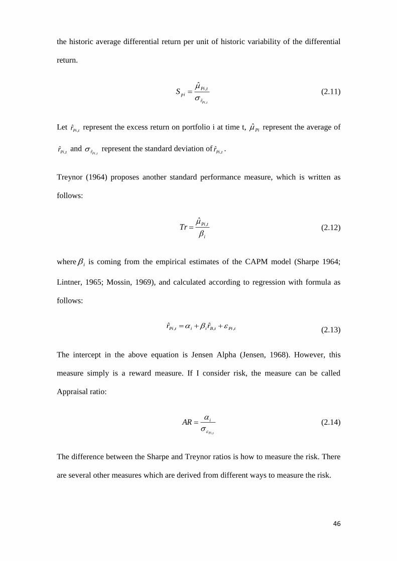
the historic average differential return per unit of historic variability of the differential

return.

tPir

tPi

piS

,ˆ

,ˆ

(2.11)

Let tPir ,

ˆ represent the excess return on portfolio i at time t, Pi represent the average of

tPir ,ˆ and

tPir ,ˆ represent the standard deviation oftPir ,

ˆ .

Treynor (1964) proposes another standard performance measure, which is written as

follows:

i

tPiTr

,ˆ

(2.12)

where i is coming from the empirical estimates of the CAPM model (Sharpe 1964;

Lintner, 1965; Mossin, 1969), and calculated according to regression with formula as

follows:

tPitBiitPi rr ,,,ˆˆ

(2.13)

The intercept in the above equation is Jensen Alpha (Jensen, 1968). However, this

measure simply is a reward measure. If I consider risk, the measure can be called

Appraisal ratio:

tPi

iAR

,

(2.14)

The difference between the Sharpe and Treynor ratios is how to measure the risk. There

are several other measures which are derived from different ways to measure the risk.

47

Konno and Yamazaki (1991) propose a ratio called expected return over mean absolute

deviation ratio:

𝐸𝑅𝑀𝐴𝐷 = 𝐸[��𝑃𝑖,𝑡] 𝐸[|��𝑃𝑖,𝑡 − 𝐸[��𝑃𝑖,𝑡]|]⁄ (2.15)

In addition, Young (1998) suggests that the expected return over Minimax ratio

𝐸𝑅𝑀𝑀 = 𝐸[��𝑃𝑖,𝑡] max(max ��𝑡=1𝑇 − min ��𝑡=1

𝑇 )⁄ (2.16)

Caporin and Lisi (2009) contribute a ratio called the expected return over the range ratio

𝐸𝐸𝑅 = 𝐸[��𝑃𝑖,𝑡] (max ��𝑡=1𝑇 − min ��𝑡=1

𝑇⁄ ) (2.17)

Modigliani and Modigliani (1997) propose a rather different measure, the Risk Adjusted

Performance, which is defined as:

𝑅𝐴𝑃 = (𝐸[��𝑃𝑖,𝑡] − 𝐸[��𝐵,𝑖])𝜎[��𝐵,𝑡]

𝜎[��𝑃𝑖,𝑡]− 𝐸[��𝐵,𝑡] (2.18)

After comparing these performance measures over a dataset that contains the stocks

included in the S&P 1500 index, Caporin and Lisi (2009) summarize that all 6 measures

provided almost similar results to the Sharpe ratio in terms of asset ranking. They

analyse rank correlation of performance measures with the Sharpe ratio over different

sample lengths. Consequently, all correlations are bigger than 0.9 excepting 3 out of 42.

2.3.2 Comparison of Sharpe Ratios

It is also important to test whether the Sharpe ratio of strategies between two portfolios

are statistically different. I calculate the p-values of these differences. The method is

suggested firstly by Jobson and Korkie (1981), and then Memmel (2003) makes the

correction simplify the test statistics without loss of its statistical properties.

48

Especially, given two portfolios, one is referred as ‘i’, and the other is portfolio k, with

Pi , Pk , Pi , Pk , PkPi , as their mean, standard deviation and covariance which are

estimated over a sample of size T-M. The null hypothesis is 0ˆ

ˆ

ˆ

ˆ

Pk

Pk

Pi

Pi

, and the test

statistic, which is asymptotically distributed as a standard normal, is:

ˆ

ˆˆˆˆˆ PiPkPkPiz

(2.19)

)ˆˆˆ

ˆˆˆˆ

2

1ˆˆ

2

1ˆˆˆ2ˆˆ2(

1ˆ 2

,

2222

,

22

PkPi

PkPi

PkPiPiPkPkPiPkPiPkPiPkPi

MT

(2.20)

In addition to p-value, the return-loss can be considered as the additional return, which

strategy k needs to perform as well as the portfolio i in terms of the Sharpe ratio. The

formula of return-loss for portfolio k is:

PkPk

Pi

PiPklossre

ˆˆ

ˆ

ˆ (2.21)

2.3.3 Risk Measure based on Drawdown

In addition to the standard deviation, there are alternative approaches to measure risk

(Biglova et al., 2004; Ortobelli et al., 2005; Rachev et al., 2008). One of possible

measures is based on Drawdowns. The Drawdown represent, at time t, the maximum

loss an investor may have suffered from 0 to t. According to order drawdown and

compute quantities, the risk measure could be such as maximum drawdown or second

largest drawdown. The relative formula is showed as follows:

Drawdown: 00,ˆmin 0,1 DrDD tPitt (2.22)

49

Maximum drawdown: T

tDD 11 min (2.23)

The Second largest drawdown: 112 min DDD T

t (2.24)

Young (1991) suggests Calmar ratio, which is the ratio between the expected return and

the maximum drawdown. Kestner (1996) introduces a Sterling ratio, which is the ratio

between the expected returns and the N largest drawdown. Burke (1994) proposes the

Burke ratio, which is the ratio between the expected return and the second order non-

central moment of the N largest drawdown. The relative formula is showed as follows:

Calmar ratio: 1

ˆ

DCR Pi

(2.25)

Sterling ratio:

w

j j

Pi

Dw

SR

1

1

(2.26)

Burke ratio:

2

1

1

21

ˆ

w

j j

Pi

Dw

BR

(2.27)

Where w is the number of value used in the computation of the risk measure. Eling and

Schuhmacher (2007) fix this w is 5. However, Caporin and Lisi (2009) conclude that

‘there is no need to consider the Sterling and Burke indices computed over different

numbers of drawdowns.

2.3.4 Risk Measure based on Quantiles

Beder (1995) concludes approaches to calculating value at risk (VaR). The VaR is

defined as the maximum loss on an asset/portfolio that can be expected over a certain

time interval with a certain degree of confidence. There are two approaches to calculate

VaR. One is related to historical data, or nonparametric approach, which uses historical

50

distribution of the returns in order to compute the appropriate loss. The other one is to

simulated data, or parametric approach, which assumes the returns follow a normal

distribution with mean and standard deviation calculated by historical data. However, a

major criticism of VaR is about subadditivity, which is described by Jorion (2007) as

‘merging two portfolios cannot increase risk’. And, he uses an example to prove that

VaR violates the principle of subadditivity. Moreover, Albanese (1997) argues that due

to a lack of subadditivity in VaR, the measure can lead to a higher concentration of

credit risk, while managing credit portfolio risk. Kidd (2012) concludes that the reason

for significant loss in a global financial crisis is to improperly understand and use VaR,

and ignore tail risk. So, a number of investors try to adopt conditional value at risk

(CVaR), which is designed to measure the risk of extreme losses.

Embrechts et al. (1999) firstly propose expected shortfall, which also is called

conditional value at risk (CVaR). This measure, an extension of VaR, represents the

expected loss of portfolio value given that a loss is occurring at or below the q-quartile.

Kidd (2012) states ‘CVaR quantifies tail risk and has been shown to be subadditive’.

Rockafellar and Uryasev (2000) show another advantage of CVaR, which is that the

optimization in portfolio risk by CVaR is easier than VaR. But, CVaR is not perfectly

and not absolutely superior to VaR, because it has defects as well. Yamai and Yoshiba

(2002) argued that in order to generate a reliable estimate, a large number of

observations are required for CVaR. Compared to VaR, CVaR is more sensitive to

estimation errors. So, Lim et al. (2010) conclude that both VaR and CVaR are used

frequently and therefore complement each other.

51

2.4 Conclusion

Since Markowitz (1952) proposes a seminal work to make the rule for constructing

portfolio, the modern portfolio management has been developed vastly in the academic

literature and in practice. Empirical studies show very poor performance of this model

with sample-based mean and variance-covariance in out-of-sample analysis. The key

problem of the failure can be attributed to errors in estimation. So, considerable effort

from literature is focused on how to handle this estimation error, and then finally to

improve the performance of portfolios.

On the one hand, a lot of literature tries to mitigate estimation errors by using the

Bayesian approach. On the other hand, equally, non-Bayesian approaches also are used

to reduce the estimation errors in a number of literatures. However, recent studies tend

to propose alternative ways to construct portfolio, beyond to Markowitz’s model and its

robust extension. I reviewed literature related to these three classes of portfolio

strategies. One of strategies, called parametric portfolio policy, needs characteristics of

currency. So, next, I reviewed literature about characteristics to determine the price of

currency.

The characteristics of currencies can be divided into two parts: financial (technical) and

fundamental (economic). The financial characteristics are from profitable currency

trading strategies, and related to change in currency price. There are three main trading

strategies in currency market. The most popular strategy in literature is referred to as

carry trade, which is to invest in currency with high interest rates and sell currency with

low interest rate. The other two are referred to as currency monument and value. The

currency monument is based on the idea of price rising after rising in the last short time.

Conversely, the currency value strategy holds that price will decrease after it increases

for a long time. So, this strategy is called long-term reverse. The fundamental

52

characteristics are the economic factors, which can determine the price of currency. The

theory of behavioural equilibrium exchange rate (BEER) has modelled how to analyse

these factors. But, literature implements this model slightly different in practice.

Lastly, the performance of portfolios needs to be evaluated by a reasonable method. The

Sharpe ratio is the most common evaluation method, because it takes account of both

return and risk. In spite of the fact that there are other alternative methods, literature has

summarised that the results from these alternatives is not different to the results from

Sharpe ratio. In addition to the standard deviation, there are other risk measures

mentioned more frequently. Drawdown is one of these risk measures. It measures the

maximum loss during the certain time periods. Another risk measure is to capture the

loss of portfolio at specific quantile. Both of the value at risk and conditional value at

risk belong to this class. Because they have their own advantages and disadvantages,

researchers would like to use both of them complementarily.

53

Chapter Three

Data

Before analysing the performance of currency only portfolio constructed using various

strategies, the methods of calculating the currency return, taking account transaction

cost are firstly introduced, followed by summarising the statistics of currency return.

The methodology of currency return calculation introduced in this chapter will be

implemented in the next three chapters, as well as the transaction cost method, but the

sample and its period might not be the same. The G10 currencies are considered as the

first dataset (9 currencies in total and another one, US dollar, as based currencies), as

they are the most 10 heavily traded currencies in the world. The corresponding countries

and area include Australia, Canada, Japan, New Zealand, Norway, Sweden, Switzerland,

UK and Euro Zone. For the second datasets, I add ‘lesser’ currencies, which are mostly

from developing countries, to bring a diversification benefit to the portfolio. The

corresponding countries include Brazil, Chile, Colombia, Czech, Egypt, Hungary,

Iceland, India, Indonesia, Israel, Mexico, Peru, Philippines, Poland, Russia, Singapore,

South Africa, Taiwan, Thailand and Turkey. So, the second data set has 29 currencies in

total.

54

3.1 Currency Return

3.1.1 Method of Calculation

To calculate currency returns, it is assumed that an investor at time t to buy currency i

for i

tS , and hold it until time t+1, and sell it at t+1 for i

tS 1, where i

tS and i

tS 1are the

price of one foreign currency unit expressed in home currency. The Investor also earns

interest at foreign countries risk free rate during t and t+1. So, the return for the investor

should be

i

t

i

t

foreign

tf

i

ti

tS

SRSR

)1( ,1

1 (3.1)

In the analysis, the plan is to include 29 currencies, which required the gathering of risk

free rates of 29 countries. However, there is difficulty in choosing an appropriate risk

free rate. In order to avoid having to make an arbitrary decision on the most appropriate

risk free rate for each country, an alternative way to calculate selected returns is

available. In the forward exchange market, the forward rate of currency is calculated as

follows (CIP, covered interest parity).

)1(

)1(

,

,

1, foreign

tf

US

tfi

t

i

ttR

RSF

(3.2)

Combining formula 1 and 2, I obtain the formula as follow.

i

tt

i

tt

us

tf

i

ti

tF

FRSR

1,

1,,1

1

)1(

(3.3)

This formula also can be explained as an investor buying currency at t for i

ttF 1, and

selling it at t+1 for i

tS 1; meanwhile the investor can earn US risk free rate, this interest

also is taken into account for forward buying and spot selling. Comparing to gather the

55

risk free rate for each country, the forward rate is easier to obtain from the database. The

advantage of using the last formula is only US risk free rate concerned. For now, the

return calculated is called ‘raw return’, but in this thesis uses excess return, which is

return over risk free rate. Therefore, risk free rate is subtracted from raw return. The

formula of excess return is as follows.

)1)(( ,

1,

1,1

1,

us

tfi

tt

i

tt

i

t

ti RF

FSr

(3.4)

In the next sub-section, the source and data description for spot rate, forward rate, risk

free rate and GDP and trade data is described.

3.1.2 Spot Rate

The spot rate data are collected from WM/Reuters FX Indexes in DataStream from 28th

October 1997 till 13th

March 2012 with weekly frequency. We, then, convert them to

USD/ foreign currency, if they are not. For the robustness check, I convert them again

to UK/foreign currency, EU/foreign currency and Japanese Yen/foreign currency. For

each currency pair, I have 751 observations in almost 15 years. According to graphic

checking, it can be confirmed that that all 29 currencies are floated to each other, with

no fixed rate over the period Selected.

3.1.3 Forward Rate

The same period forward rate data is collected from DataStream. However, in the case

of some currencies, there are no forward rates available from 28th

October 1997. So, I

simulate the forward rate for these currencies and period of absence by using formula

3.2 in the last subsection. The question now is that not all countries have 3-month T-bill

from DataStream. So, pairs of following interest rate shown in Table 3.1 are used

instead of 3-month T-bill.

56

Forward rates for the period after 23th

March 2004 are simulated, and compared to

actual forward rates. The difference between the calculated forward rates and the actual

forward rates is calculated. The percentages are computed by these differences over the

actual forward rates. The average and standard deviation of these percentages are

demonstrated in Figure 3.1. From the figure, all averages and standard deviations of

percentages, which are no more 0.7%, can be considered to be very small. In addition to

statistical analysis, the calculated forward rates along with the actual forward rates are

graphed. As per Figure 3.2, for each currency, the line which represents the forward rate

from DataStream coincides with the line which represents the calculated forward rate.

So, I can confirm that there is no significant difference between the two rates and the

two rates are almost the same. It can be assumed that the simulated forward rates are

reliable, 751 observations of forward rates covering a 15 year period were reviewed.

57

Table 3.1 List of currencies with absent forward rate

The first column of table lists currencies that do not have forward rate in DataStream. The next column provides the

date of forward rate is available. The last two columns lists the names of risk free rates used for local countries and

corresponding name of risk free rates for the US. All risk free rates are collected from DataStream with weekly

frequency, and then divided by 52 to obtain weekly rate.

Currencies Absence until Interest rate Corresponding US interest rate

Iceland Krona 23/03/2004 Treasure bond yield 10 years Treasure bond yield 10 years

Israeli Shekel 23/03/2004 T-bill secondary 3 month T-bill secondary 3 month

Brazilian Real 23/03/2004 Saving account CD second market 6 month

Colombian Peso 23/03/2004 Fixed term deposit Conventional fixed mortgages

Egyptian Pound 23/03/2004 91 Day T-Bill Treasury constant MAT 3 month

Peru New Sol 23/03/2004 Interbank interest rate Average of interbank interest rate

Russian Rouble 23/03/2004 Interbank 8 to 30 day Interbank 1 MTH

Chilean Peso 23/03/2004 CD 30 Days CD 1 month

58

Figure 3.1 Statistics of percentage of difference between calculated FWD and quoted FWD

over quoted FWD

The purpose of this figure is to compare the calculated forward rates with the quoted forward rates for the eight

currencies, which do not have forward rate for the part of sample period. The method used is to firstly take the

difference between two values, and then calculate the percentage of this difference over quoted forward rates. Finally,

this figure demonstrates the average and standard deviation of this percentage.

0.00%

0.10%

0.20%

0.30%

0.40%

0.50%

0.60%

0.70%

Average

Standard Deviation

59

Figure 3.2 Comparison of calculated FWD with quoted FWD

This figure compares the forward rate from source with the calculated forward rate. The currencies reported here are

that their forward rates are not available for the whole sample period. And, the period is from 2014 to 2012, which

the forward rates of these currencies are available for. For each currency, the blue line (referred as WMD) is the

forward rate from WM/Reuters FX Indexes in DataStream, and the red line (referred as calculated) represents the

forward rate I calculated by

)1(

)1(

,

,

1, foreign

tf

US

tfi

t

i

ttR

RSF

.000

35.0

004

.000

45.0

005

.000

55.0

006

01jan2004 01jan2006 01jan2008 01jan2010 01jan2012

WMR Calculated

Colombian Peso

.16

.17

.18

.19


WMR Calculated

Egyptian Pound

.25

.3.3

5.4


WMR Calculated

Peru New Sol.0

25.0

3.0

35.0

4.0

45


WMR Calculated

Russian Rouble

.005

.01

.015

.02


WMR Calculated

Icelandic Krona

.2.2

2.2

4.2

6.2

8.3


WMR Calculated

Isreal Shekel

.3.4

.5.6

.7


WMR Calculated

Brazilian Real

.001

4.0

016

.001

8.0

02.0

022

.002

4


WMR Calculated

Chilean Peso

60

3.1.4 Risk Free Rate

In this thesis, risk free rates are required in order to calculate currency return and sharp

ratio. There are risk free rates of three countries and one zone collected from

DataStream for the same period with weekly frequency. US risk free rates are used for

base samples. For robustness checking, Japanese, UK, and Euro zone risk free rates are

necessary. US 3 month T-bill interest rate is used for analysis of US investors’

perspective, UK 3 month gilt for analysis of perspective of UK investors, and Japanese

commercial paper 1 month for analysis of perspective of Japanese investors. As far as

Euro zone investors are concerned, it is a more complicated process. There is a need to

obtain weights of the countries within the Eurozone. Fortunately, the European Central

Bank (ECB) provides this kind of weights, and updates them yearly on its website. The

ECB calculates these weights based on GDPs, and use them to calculate Harmonised

Index of Consumer Prices (HICP) for Eurozone by a weighted average of countries’

price index. After reweighting, the six largest weights add up to 1. This is then

followed by collecting these six countries’ risk free rates from DataStream. The home-

made euro risk free rate is calculated by using the weighted-average method. Table 3.2

demonstrates the re-weighted weights and the names of risk free rate used for these six

countries.

61

Table 3.2 Weights and names of risk free rate of six euro countries

This table lists two components of euro risk free rate in my calculation. One is weights, which obtained from the

European Central Bank’s website. I reweight six largest weights of countries adds to one. Other one is the name of

risk free rate for each country.

France Germany Italy Spain Netherland Belgium

1997 23.7% 37.3% 19.6% 9.6% 5.7% 4.1%

1998 23.7% 37.3% 19.7% 9.6% 5.7% 4.1%

1999 22.8% 37.3% 20.3% 9.8% 5.5% 4.3%

2000 22.5% 37.4% 19.7% 9.8% 6.1% 4.3%

2001 23.0% 34.7% 21.0% 11.7% 5.9% 3.7%

2002 22.9% 34.3% 21.6% 11.5% 5.8% 3.8%

2003 23.0% 33.5% 21.5% 12.2% 6.1% 3.7%

2004 23.3% 32.8% 21.7% 12.5% 6.0% 3.7%

2005 23.3% 32.7% 21.6% 12.8% 5.9% 3.7%

2006 22.9% 32.4% 21.5% 13.5% 5.9% 3.8%

2007 23.5% 32.0% 20.7% 13.9% 6.0% 3.9%

2008 23.5% 31.0% 21.3% 14.6% 5.7% 3.9%

2009 23.8% 30.2% 21.4% 14.8% 5.9% 3.9%

2010 24.2% 30.4% 21.1% 14.6% 5.9% 3.7%

2011 24.1% 30.2% 21.5% 14.8% 5.6% 3.8%

2012 23.9% 30.8% 21.1% 14.4% 5.7% 4.1%

Name France T-Bill 3

Month

Money market 3

month

Italy T-Bill AUCT.

GROSS 3 MONTH

SPAIN T-Bill 1-

3 MONTH

NTHRLAND EU-

GLDR 3M

BELGIUM

TREASURY BILL 3

MONTH

62

3.1.5 GDP and Trade

In the CAPM world, for the equity, the optimal strategy is the value-weighted market

portfolio. So, in this thesis, I attempt to identify market portfolio. But, due to no direct

value for the currencies, indirect methods are used to determine the currency value. For

the currency market, the total value of currency can be considered as the value of this

country, which can be represented by GDPs. Alternatively, the currency rate is closely

related to trade. The change in currency rate affects bilateral trade, and the sum of

import and export may be considered as value of currency. So, GDPs and the sum of

bilateral trade is used to construct two benchmark market portfolios. As a result of a

delay in releasing GDP data and trade from national statistics authorities, the previous

year’s GDPs and trade data obtained from DataStream, is used to calculate weights for a

whole currency year returns. GDPs collected are under expenditure approach at current

market price, but is dominated by local currencies. I therefore firstly, convert them to

US dollars using year end spot rate. In the robustness checking, the trades of most

members of the Eurozone with developing countries are not available, so I do not

construct trade portfolio of 29 currencies for euro investor.

3.2 Summary Statistics

In this section, the statistics of currency returns, risk free rate and GDP and trade

weights all related to the perspective of US investors are summarised. From other

investors’ perspectives, the conclusions of statistics are almost similar to what I

conclude from US investors.

63

3.2.1 Currency Return

The statistics of returns on 29 currencies are well documented in Table 3.3. From this

table, the Polish zloty has the highest average weekly return, while the new Turkish lira

has lowest return of -2.41% (annualized return of -125%). Because of a chronic

inflation experienced in Turkey from the 1970s through to the 1990s, the lira

depreciated in value. This also led to the highest standard deviation of returns of the lira.

According to the maximum and minimum return during sample period, the Russian

rouble can be considered as very volatile with maximum return of 99% and minimum

return of -45%. This can be partly attributed to the 1998 Russian financial crisis

resulting in a 70% drop in value against the US dollar. In addition to the new Turkish

lira and Russian rouble, there are several other currencies with the anomalously kurtosis

and skewness, which indicate that the distribution of returns of these currencies

significantly deviate from the norm. These currencies, which include Icelandic krona,

Brazilian real, Egyptian pound, Peru new sol and Philippine peso, went through the

same challenges as the Russia and Turkey, experiencing a huge drop in value due to

rapid economic decline. In sharp contrast, the G10 currencies do not have an anomaly

as evidenced by the available statistics. A critical analysis of available data from year to

year shows the anomalies of emerging currencies vanishing with no immediate financial

impact. Ccorrelations are also analysed for each full calendar year. All correlations are

less than 0.85 I can therefore conclude that there are no clearly defined correlations

between any two currency returns.

64

Table 3.3 Statistics of 29 currencies returns

This table shows the results of statistics of 29 currencies returns for the time period from 4/11/1997 to 13/3/2012.

‘Mean’ represents the average return, and ‘SD’ represent standard deviation of currencies returns. The high moments

of returns are reported in column 7 and 8, which use ‘SK.’ and ‘KU.’ to represent skewness and kurtosis respectively.

The last two columns give maximum and minimum returns in the period for each currency. Because the weekly

return is calculated before, the results are also based on weekly frequency. But, for the convenience to compare with

other data, I also report the annualized mean and standard deviation, which is referred to as ‘Annualized Mean’ and

‘Annualized SD’ respectively in the table. The process of annualizing used is simple transformation. For example,

the mean is multiplied by 52 to get annualized mean, and standard deviation is multiplied by square root of 52 to get

annualized standard deviation.

Name NO.of Ob Mean Annualized

Mean SD

Annualized

SD SK. KU. MAX MIN

AUSTRALIAN $ 750 0.16% 8.47% 1.85% 13.37% -0.16 4.26 7.14% -9.36%

CANADIAN $ 750 0.11% 5.62% 1.35% 9.75% 0.55 9.32 2.08% -6.35%

ICELANDIC KRONA 750 0.06% 3.25% 2.12% 15.27% 2.97 48.72 1.61% -10.56%

ISRAELI SHEKEL 750 0.10% 5.34% 1.11% 8.01% -0.50 2.32 3.55% -5.19%

JAPANESE YEN 750 0.05% 2.77% 1.47% 10.61% 0.69 3.86 10.25% -5.88%

NEW ZEALAND 750 0.16% 8.18% 1.99% 14.33% -0.14 2.76 9.79% -10.56%

NORWEGIAN

KRONE 750 0.12% 6.05% 1.67% 12.07% -0.28 1.49 3.29% -7.44%

SINGAPORE 750 0.06% 3.19% 0.85% 6.11% -0.01 6.11 5.67% -4.54%

SWEDISH KRONA 750 0.07% 3.87% 1.68% 12.11% -0.26 1.12 4.06% -7.81%

SWISS FRANC 750 0.08% 4.22% 1.50% 10.85% 0.03 1.12 4.48% -6.52%

UK £ 750 0.07% 3.56% 1.30% 9.37% -0.24 2.32 2.54% -7.99%

EURO 750 0.07% 3.80% 1.44% 10.38% 0.20 1.93 2.67% -4.15%

BRAZILIAN REAL 750 0.10% 5.01% 2.38% 17.18% -1.90 17.95 13.03% -23.34%

CHILEAN PESO 750 0.03% 1.38% 1.48% 10.69% -0.12 1.90 2.10% -6.81%

COLOMBIAN PESO 750 0.13% 6.68% 1.70% 12.28% -0.26 5.56 5.30% -8.78%

CZECH KORUNA 750 0.16% 8.28% 1.81% 13.08% -0.38 1.32 4.40% -8.33%

EGYPTIAN POUND 750 0.09% 4.59% 0.78% 5.62% -13.75 276.95 1.08% -16.39%

HUNGARIAN

FORINT 750 0.18% 9.38% 2.03% 14.66% -0.57 2.72 2.17% -12.13%

INDIAN RUPEE 750 0.09% 4.45% 0.83% 6.00% -0.43 6.40 2.83% -4.36%

INDONESIAN

RUPIAH 750 0.11% 5.60% 3.63% 26.20% 0.04 23.50 31.97% -26.61%

MEXICAN PESO 750 0.16% 8.08% 1.42% 10.26% -0.05 6.38 3.30% -8.93%

PERU NEW SOL 750 0.15% 8.00% 0.81% 5.84% 2.25 23.22 1.85% -4.48%

PHILIPPINE PESO 750 0.12% 6.35% 1.28% 9.25% -1.20 22.52 6.66% -12.58%

POLISH ZLOTY 750 0.20% 10.37% 2.03% 14.61% -0.79 3.38 3.22% -10.67%

RUSSIAN ROUBLE 750 0.11% 5.73% 4.53% 32.65% 11.68 320.07 98.86% -44.92%

SOUTH AFRICA

RAND 750 0.16% 8.19% 2.31% 16.64% -0.55 3.29 4.16% -14.76%

TAIWAN NEW $ 750 0.04% 1.90% 0.66% 4.77% -0.10 4.22 3.16% -3.40%

THAI BAHT 750 0.13% 6.76% 1.35% 9.75% 0.63 29.84 13.73% -11.54%

NEW TURKISH LIRA 750 -2.41% -125.26% 11.48% 82.78% -3.81 13.31 2.23% -57.96%

65

3.2.2 Risk Free Rate

US 3 month T-bills have a weekly return with mean of 0.05%, standard deviation of

0.04%, skewness of 0.13, kurtosis of -1.51, maximum return of 0.12% and minimum

return of almost 0. A tiny standard deviation indicates that the risk is very small, so,

which can be considered as risk free rate. As minimum return and positive skewness

show that all return are above 0, this is rational for the risk free rate. A negative kurtosis

indicates a relatively flat distribution.

3.2.3 GDP and Trade

The first chart of Figure 3.3 documents average weights of each currency in G10

currencies for GDP and trade portfolios, and the second chart shows this in 29

currencies. Because of no significant difference between the weights of each year, the

average weights are representative. Due to being members of the North America Free

Trade Association, Canada and Mexico have the largest weights in trade portfolio, but

small weights in GDP portfolio, while the euro zone has the largest weights in GDP

portfolio for both G10 and 29 currencies. According to the above factors, the GDP and

trade portfolios have significantly different weights in some countries, which may lead

to significantly different returns for these two portfolios. One disadvantage of these two

portfolios is transaction cost of rebalancing, compared to value-weighted portfolio in

equity with no rebalancing cost.

66

Figure 3.3 Average weight of each currency for GDP and Trade portfolios

This bar chart reports average percentages of each country/area’s GDP and trade volume to/from US over sum of all

currencies/area’s GDP and trade volume to/from US. I firstly compute these percentages for every year from 1997 to

2012, then reports only average of them. The percentages reported can be considered as average weights of each

currency for GDP and Trade portfolios. There are two datasets used in this thesis. So, the first chart reports the results

for the portfolios containing only G10 currencies. The second consider portfolios containing all 29 currencies.

0.00%

10.00%

20.00%

30.00%

40.00%

50.00%

60.00%

G10 Currencyies

GDP

Trade

0.00%5.00%

10.00%15.00%20.00%25.00%30.00%35.00%40.00%

Euro

Jap

anes

e Y

EN

UK

£

Can

adia

n $

Bra

zilia

n r

eal

Me

xica

n p

eso

Ind

ian

ru

pee

Au

stra

lia $

Ru

ssia

n R

ou

ble

Swis

s Fr

ance

New

Tu

rkis

h li

ra

Taiw

an N

ew $

Swed

ish

kro

na

Ind

on

esi

an r

up

iah

Po

lish

zlo

ty

No

rwe

gian

kro

ne

Sou

th

Afr

ica

Ran

d

Thai

bah

t

Isra

eli s

he

kel

Co

lom

bia

pes

o

Sin

gap

ore

Cze

ch k

oru

na

Ch

ilean

pe

so

Egyp

tian

po

un

d

Ph

ilip

pin

e p

eso

New

Zea

lan

d $

Hu

nga

rian

fo

rin

t

Pe

ru n

ew s

ol

Ice

lan

dic

kro

na

29 Currencies

GDP

Trade

67

3.3 Turnover and Adjustments for Transaction Cost

Considering transaction cost bigger than zero, any changes in portfolio weights will

result in reduced returns. The portfolio turnover is computed, defined as the fraction of

invested wealth traded at rebalance date. The formula is shown as follows:

𝜏 =1

𝑇−𝑀∑ ∑ (|��𝑘,𝑗,𝑡+1 − ��𝑙,𝑗,𝑡+|)𝑁

𝑗=1𝑇−𝑀𝑡=1 (3.5)

1,,ˆ

tjkw is the weights of portfolio k in asset j at time t+1, and tjkw

,,ˆ is weights of the

portfolio k before rebalancing at t+1 in asset j. Note that if one dollar is invested in

portfolio at time t, the investment in asset j will be 1,,, 1ˆ tjtjk rw dollar at time t+1

before rebalancing. Hence, before the portfolio k is rebalanced, the weight in asset j at

time t+1 is:

N

j tjtjk

tjtjk

tjkrw

rww

1 1,,,

1,,,

,,1ˆ

1ˆˆ (3.6)

Increases in portfolio turnover can lead to portfolio performance after transaction cost to

deteriorate. According to equation 3.4 and 3.5, turnover increases with the variance of

the portfolio weights across time, and these are dependent on the sampling variation in

t and t , which may change with length of estimation window.

As far as transaction costs are concerned, Lesmond et al. (2004) argue that they are

relevant to assess the performance of an investment strategy. So, one valid concern is

about performance after taking account of these costs. To calculate transaction cost, one

half of the bid-ask spread is used as a percentage of the min-quote, applied by Barroso

and Santa-Clara (2011), although this method may overstate transaction costs (Mancini

et al., 2013). Transaction cost of currency I at time t is calculated as:

68

bid

tti

ask

tti

bid

tti

ask

tti

tiFF

FFc

1,,1,,

1,,1,,

,

(3.7)

Portfolio returns are then adjusted for these costs as:

1)1)(ˆ1(~,,,1,, tjPitj

N

jtPitPi crr (3.8)

In which tjPi ,, are turnover for asset j in portfolio I at time t.

3.4 Conclusion

In this section, two common methods are introduced, which will then be applied into of

the rest of the chapters. The first one is a method of calculating the return of currency.

To enable calculation and data collection to be easy, the forward rate is used to replace

the spot rate at time t+1. So, the calculation for each currency successfully avoids

gathering all risk free rates from different countries, but, only concerns US risk free rate.

The second method introduced is how to take account of transaction cost into a

portfolios return. The turnover is calculated at the end of each time point as sum of

changes in weights for rebalancing. Transaction cost of currency is not fixed, but is

dependent on bid and ask forward rate. The return of portfolio after transaction cost is

obtained followed by computation of, turnover and transaction.

The data is collected weekly, mainly from DataStream. But, some forward rates are not

available for the sample period. Covered interest parity is used to calculate the

unavailable forward rates. Moreover, after statistics and graphing check, the calculated

forward rate can be considered as a reliable source. According to the statistics of

currency return, the G10 currencies have a more stable performance than ‘lesser’

currencies and the correlations confirm that all 29 currencies are not highly correlated to

each other.

69

Chapter Four

Currency Portfolio Management: Passive Portfolios vs

Naïve Portfolio

4.1 Introduction

International investment has become increasingly important since the advent of free

floating exchange rates and the removal of capital controls. The risk inherent to foreign

exchange rates can eliminate or substantially reduce the profit made on an international

investment. Therefore, instruments, such as forwards and options, were used to hedge

this risk (Black, 1989); (Glen and Jorion, 1993); (Larsen Jr and Resnick, 2000);

(Topaloglou et al., 2008); (Fonseca et al., 2011). However, increasingly currencies are

thought of as an asset in their own right. Levy and Sarnat (1978) report the achievement

of significant gains from holding foreign currencies from investor US investor

perspective. They also analyse and confirm the gains from diversification for only

currencies portfolios and portfolios of foreign currency and country’s stock index.

In contrast, the studies which consider passive portfolio investment among currencies

are not many. A most relevant research about passive currency-only portfolios is written

by Levy and Sarnat (1978). They simply apply basic idea of modern portfolio theory by

sample mean and standard deviation to construct set of efficient portfolios. A number of

robust models and alternative methods have been created to improve and enhance the

performance of Markowitz model. But, few researches apply these methods into

construction of currency-only portfolio.

70

This chapter adds to this literature by considering a number of portfolio optimization

methods applied to currency-only portfolio. As mentioned in preceding paragraphs, the

gap in literature is passive optimization for portfolio with currency only. This study fills

this gap, which is important to investors who desire to take a position in foreign

currencies, due to nature and magnitude of their economic activities, such as central

banks, international investment trusts, and large multinational corporations.

Portfolio optimization has been extensively studied in equity and bond markets, both

analytically and empirically. Since Markowitz (1952) derived the optimal rules for

allocating wealth with risky assets, a number of studies focused on this topic resulting in

the development of this model with some adjustments. Other studies tried to create

alternative methods for constructing portfolio to beat the market. All these models have

been empirically applied to the stock market or bond market for testing efficiency.

Problem with estimation error attracted considerable effort to solve it with purpose of

improving the performance of the Markowitz model. James and Stein (1961) and Jorion

(1986) design a shrinkage form to handle the error in estimating expected returns

Pástor (2000) and Black and Litterman (1992) improve an asset pricing model to

estimate the expected return. Goldfarb and Iyengar (2003) introduce the ‘robust’

portfolio rules. Kan and Zhou (2007) design their rules to optimally diversify portfolio

across market and estimation risk. Some approaches are to constrain the portfolio

weights, e.g. Frost and Savarino (1988) impose the short selling constraints for the

portfolio optimization. The purpose of these methods is to improve the properties of the

portfolio weights, and they did.

However, DeMiguel et al. (2007) show that in the equity market, it is very difficult to

beat the naïve portfolio. In their analysis, they use various US indices and international

indices, and consider various asset-allocation models all derived from Markowitz’s

71

model. And then, they compared the performances of the optimal portfolios against

naïve portfolio, and summarised that no single model consistently outperforms the naïve

portfolio.

Alternative methods are developed based on other thoughts with same goal of

improving the out of sample performance of portfolio. Maillard et al. (2008) introduce a

new optimal strategy called equally-weighted risk contribution, which considers the

amount of risk an individual contributed to portfolio. From their empirical evidence

regarding two asset classes, equity US sectors portfolios and agricultural commodity

portfolios, naïve portfolio is inferior in terms of performance and for any measure of

risk, and minimum variance portfolio achieves higher Sharpe ratio but expose to higher

drawdown as well. However, in the class of global diversified portfolio dataset, the

ERC strategy has the best performance in terms of Sharpe ratio.

The conclusions made from other asset classes may not be consistent with that from

currency market. Jylhä and Suominen (2011) prove that profit-seeking capital in

currencies has a relatively minor role during most of the floating exchange rate area.

Taylor (1982) also states that the most important actors in the currency market, central

banks; do not seek profits at all. This characteristic of currency market is not for other

asset classes. Therefore, the conclusions may be different.

In this chapter, as already indicated, a number of passive portfolio strategies are applied

into the currency market. In this chapter, the main objective is to analyse the

performance of various optimal portfolio models for the class of currency exchange

market, and find out the most efficient strategy for investors. To do this, an evaluation

of the out-of-sample performance of various portfolio construction policies is done. The

policies include sample-based mean-variance portfolio policy and its extension, which

are applied in DeMigual’s research (2007), equally-weighted risk contribution model,

72

which was introduced by Maillard et al. (2008), equally-weighted portfolio (1/n or

naïve portfolio), GDP portfolio, and trade portfolio. Similar to DeMigual’s (2007)

research, this analysis relies on a ‘rolling sample’ approach, but with an estimation

window of 5 years. I also take account of transaction cost, and compare the results

before and after transaction cost. In robustness check, the estimation window is changed

to 1, 3 and 10 years, and results analysed from foreign investors’ perspective (UK,

Japan and euro zone).

In contrast to DeMigual’s (2007) research, methodologies related to the risk

management are applied in order to evaluate the performance of different portfolio

models. The reason of focusing more on risk is that investors regardless of speculator or

hedger in Forex do not like high risk exposure. Considering investor systemic risk, the

Treynor ratio and Jansen alpha are also accepted in performance evaluation. Because

Dunis et al. (2011) concludes good performance of lesser currencies in most case of

portfolios, both cases also need to be considered with and without lesser currencies. In

contrast to their method of adding lesser currencies one by one, two datasets are used.

One consists of G10 currencies, which are considered to be the 10 most liquid

currencies in the world. Another one consists of 29 currencies around the world. This

setting of datasets is more practical in the real world.

The first finding of this chapter is that, out of 12 different portfolio models, the sample-

based mean-variance portfolio perform badly for out-of-sample analysis in all terms

including Sharpe ratio, VaR, maximum drawdown (expose to extreme risk). Although

this finding was shown in the literature with regard to other asset classes, such as equity

in DeMigual’s (2007) research, this is proven to be also true using evaluation methods

related to risk across datasets of currency market with and without lesser currency.

73

The second finding is that the short sale constraints help but not a lot. Although,

imposing constraints on most of strategies lead to a modest improvement, these

improvements do not change portfolio rankings. As far as turnover is concerned, the

constraints substantially reduce it, but the benchmark portfolios still have the lowest

turnover among the 12 portfolios. This is almost consistent with DeMigual’s (2007)

findings. They state that unconstrained policies perform much worse than any of the

strategies that constrain short sales. But, in this chapter, one constrained policy appears

to be lower Sharpe ratio than unconstrained one.

The third finding is that 1/N portfolio (naïve) performs reasonably well. Despite the fact

that the 1/N portfolio does not have the best performance in sharp ratio, CEQ and risk

measures, it has a very low turnover, which would help the portfolio exceed others

perhaps if I take account of transaction costs. Furthermore, in three benchmark

portfolios (naïve, GDP and trade), the 1/N portfolio has the highest Sharpe ratio. In

addition, 1/N portfolio’s return-loss and p-value of Sharpe ratio against others prove

that the performance of 1/N portfolio is not far behind others. This indicates that the

main conclusion of DeMigual et al (2007) could be accepted by an asset class of

currency exchange market.

The next finding is that the minimum variance portfolio works best. In general, this

portfolio has the best performance among portfolios in terms of all measures except

turnover, although, regarding the dataset with 29 currencies, the minimum variance

portfolio have slight low CEQ than ERC portfolio. Comparing to the analysis of

Mailard et al (2008), the same conclusions are reached, which are the worst

performance for naïve portfolio and the best for minimum variance portfolio for ERC

strategy. In addition, it can be said that ERC portfolio has much lower turnover than

minimum variance portfolio. Although DeMigual et al (2007) do not form an opinion

74

on the performance of minimum variance portfolio, the tables in their research show

that minimum variance portfolio performs best for most of the datasets in Sharpe ratio

and CEQ. This is consistent with the conclusion reached in this thesis.

The final finding is that Transaction cost does not seriously affect the results from

before transaction cost analysis. The main evaluation indexes have no significant

change after taking account of transaction costs for all portfolio models except three

models. The exceptions include sample mean-variance (mv) portfolio, Bayes-stein

shrinkage (bs) portfolio and combination portfolio with mean-variance and minimum

variance (mv-min). The relative large change of these three portfolios is due to large

turnovers. However, the change does not have impact on my results, because of poor

performance of these three portfolios from before transaction cost analysis. The large

turnovers make performance even poor after transaction cost analysis. According to six

main evaluation indexes, the results from before and after transaction cost are almost the

same. The minimum variance (min) portfolio can be considered as the best performance

portfolio. The naïve portfolio has relative good performance, and the sample mean-

variance portfolio performs badly. Although there are inconsistent results for several

samples, they are very small, and it can be concluded that there is no effect to results

after taking account of transaction cost.

The rest of the chapter is organised as follows. In section 4.2a description of passive

portfolio strategies is made as well as the evaluation methods used in this chapter.

Section 4.3 presents the results from empirical work while section 4.4 concludes.

4.2 Empirical Framework

In this section, a brief description of each portfolio optimisation model and performance

measure is provided. The detail is introduced in Chapter Two; Literature review.

75

4.2.1 Portfolio Construction Models

4.2.1.1 Naïve Portfolio (‘1/n’), GDP Portfolio (‘GDP’) and Trade Portfolio

(‘trade’)

Naïve portfolio involves holding a portfolio weight N

wew

t

1 in each of the N risky assets.

GDP and trade portfolios are applied by using weights of GDP and sum of export and

import of corresponding countries, respectively. Due to a delay in releasing data of

GDPs and trade from national statistics authorities, last year’s data is used to calculate

weights for a whole current year returns. These strategies completely ignore the data,

and are considered as one of the benchmarks in evaluation performance.

4.1.3 Sample-based Mean-variance Portfolio (‘mv’)

Markowitz (1952) derives the mean-variance portfolio, which suggests that investors

optimise the trade-off between the mean and variance of portfolio return. To implement

his model, sample mean and sample covariance matrix of historic excess return are

plugged into the original formula provided by Benninga (2000). Note that this approach

completely ignores the possibility of estimation error.

tt

ttmv

tw

ˆˆ

ˆˆ

1

1

Ω

Ω (4.1)

In which Ω is N*N variance-covariance matrix of historical excess returns, is N*1

vector of mean of historical excess returns, and N is number of currencies.

4.2.1.3 Bayes-Stein Shrinkage Portfolio (‘bs’)

In order to solve estimation error, this portfolio combines both a shrinkage approach

and a traditional Bayesian estimation, and hence, it is known as the ‘Bayes-Stein’

76

portfolio (James and Stein, 1961). In this analysis, this model is implemented by using

the estimator proposed by Jorion (1986). He takes the ’grand mean’ to be the mean of

minimum-variance portfolio, and solve out the shrinkage estimator. The formula used in

this chapter is shown below.

minˆˆ)ˆ1(ˆ bs

(4.2)

In which min is the mean of the minimum-variance portfolio and shrinkage estimator

can be re-formed as follows.

)ˆ(ˆ)'ˆ()2(

2ˆmin1min

ΩMN

N (4.3)

NN

NNbs

MMM 1ˆ'1

'11

)ˆ1(

ˆ

ˆ

11ˆˆ

1

ΩΩΩ

(4.4)

In which is defined as

ˆ1

ˆ

M . M is number of observations, N is number of assets,

𝟏𝑵 is vector of ones, bs and bs

Ω are estimators of N*1 vector of expected return and

N*N covariance matrix. The portfolio weight obtained by bs and bs

Ω is:

bs

t

bs

tN

bs

t

bs

tbs

tw

ˆˆ1

ˆˆ

1'

1

Ω

Ω (4.5)

4.2.1.4 Optimal Three Fund Portfolio (‘mv-min’)

Kan and Zhou (2007) propose to invest in another risky portfolio to diversify the

estimation risk which sample tangency portfolio has. They choose the minimum-

variance portfolio as another risky portfolio, because the weights of minimum-variance

portfolio are just relative to covariance matrix but not sample means. The weights will

be estimated with higher accuracy. The form of a portfolio rule is as follows:

77

Nttt

mv

t dcx 1ˆˆˆ1ˆ 11min ΩΩ

(4.6)

In which c and d maximise utility of a mean-variance investor. So, Kan and Zhou (2007)

derive the following formula to decide the weights.

Ntt

a

tt

a

amv

t

MNM

N

MNMM

NMNMx 1ˆˆ

ˆˆˆ

ˆ

ˆ

)2(

)4)(1(ˆ 1min

2

1

2

2min

ΩΩ

(4.7)

Defining the Incomplete Beta function:

dyyybaBbx

a

x

1

0

1 )1(),(

(4.8)

2

1,

2

1

)ˆ1()ˆ(2)1(ˆ)1(ˆ

)ˆ1/(ˆ

2

2

22

1

222

22

NMNMB

M

NNM

MN

a

(4.9)

min1'min2 ˆˆˆˆˆˆttttt

Ω (4.10)

The weights of this three fund portfolio are:

min'

minmin

ˆ1

ˆ

mv

tN

mv

tmv

tx

xw (4.11)

4.2.1.5 Mixture of Equally Weighted and Minimum-variance Portfolio (‘1/n-min’)

Because expected returns are more difficult to estimate than covariance, DeMiguel et al.

(2007) is motivated to consider a portfolio which combines 1/n portfolio with

minimum-variance portfolio. The portfolio is considered as follows.

1ˆ1..ˆ11 min/1'1min/1 n

tNtN

n

t wtsdN

cw Ω (4.12)

78

Again, c and d are chosen to maximise the expected utility of a mean-variance investor,

and is derived as follows:

NtNdc 1ˆ11 1' (4.13)

NtNNtNNtNNtN

NtNNtN

NMMNkNMN

MNNMd

1ˆ1)1ˆ1(21ˆ121ˆ12

)1ˆ1(1ˆ111''1'21'2

2'1'

ΩΩΩΩ

ΩΩ (4.14)

421

22

NMNMNM

MMk (4.15)

4.2.1.6 Short-sale-constrained Portfolio (‘ss’)

We also consider the above strategies with constraints of short selling, which impose an

additional non-negativity constraint on the portfolio weights in the corresponding

optimization problems.

Jagannathan and Ma (2003) find that, with a constraint on short sales, ‘the sample

covariance matrix performs almost as well as those constructed using factor models,

shrinkage estimators or daily return.’ As a result of this finding, the performance of the

models which have been developed to deal with estimation errors on covariance matrix,

such as Best and Grauer (1992), are not evaluated.

4.2.1.7 Equally-weighted Risk Contribution Portfolio (‘erc’)

Neukirch (2008a) supports the equally-weighted risk contribution portfolio (ERC). The

idea is to equalise risk contribution of components of the portfolio. The risk

contribution can be calculated by product of weight with its marginal risk contribution.

Maillard et al. (2008) implement ERC into practice (equity US sectors portfolio,

agricultural commodity portfolio and global diversified portfolio).

Starting to set an original vector of weights tw , the risk of the portfolio is

79

tttt ww Ω' (4.16)

In which t is N*N variance and covariance matrix. The marginal contribution is

ti

ji tijtjtiti

ti

tw

w

ww

wti

,

,,

2

,,

,,

(4.17)

Where tiw ,is weight of asset i, 2

,ti is variance of asset i, tij , is covariance of asset i and

asset j. In vector for,

ttt

ttt

ww

w

Ω

Ω

ˆ

ˆ

' (4.18)

So, the risk contribution of the asset i is:

tiwtiti w

,,, (4.19)

The ERC problem can be written as follows:

𝑤𝑡𝑒𝑟𝑐 = {𝑤𝑡

𝑒𝑟𝑐 ∈ [0,1]; 𝑤𝑡𝑒𝑟𝑐′

𝟏𝑁 = 1; 𝜎𝑖,𝑡 = 𝜎𝑗,𝑡} 𝑓𝑜𝑟 𝑎𝑙𝑙 𝑖 𝑎𝑛𝑑 𝑗 (4.20)

4.2.2 Performance Evaluation Method

4.2.2.1 Traditional Performance Measures

In this chapter, in order to assess the portfolio performance, the ex-post Sharpe ratio

(Sharpe, 1966, 1994), is used first; which indicates the historic average differential

return per unit of historic variability of the differential return. I let tPir ,ˆ represent the

excess return on portfolio i at time t, Pi represent the average of tPir ,ˆ and

tPir ,ˆ

represent the standard deviation of tPir ,ˆ . So, the ex-post Sharpe ratio can be written as

follows.

80

tPir

tPi

piS

,ˆ

,ˆ

(4.21)

We use Memmel’s method to test the statistical difference of Sharpe ratios between

each strategy and naïve portfolio1. In addition to Sharpe ratio, I also apply Treynor

measure and Jansen Alpha to evaluate the performance. The benchmark for calculating

i is GDP portfolio, which is more like market portfolio.

The return-loss also is computed as follows:

PiPi

ew

ewPilossre

ˆˆ

ˆ

ˆ (4.22)

4.2.2.2 Certainty-Equivalent (CEQ)

We define CEQ return as the riskless rate that an investor is willing to accept rather than

adopting a risky portfolio i. The formula is given as:

2ˆ2

ˆPiPiiCEQ

(4.23)

The results reported are for the case of =5, which is the risk aversion of an investor.

However, I also calculate CEQ in the case of 1 and 10 (without reporting),

4.2.2.3 Maximum Drawdown

The maximum drawdown is the maximum loss an investor may have suffered during

whole period. The relative formula is shown as follows:

Drawdown: 00,ˆmin 0,1 DrDD tPitt

1 Specially, given two portfolios, one is 1/n portfolio referred as ‘ew’, another one is portfolio i, with

ew ,Pi ,

ew , Pi ,

ewPi , as their mean, standard deviation and covariance which are estimated over a sample of size T-M. The null

hypothesis is 0ˆ/ˆˆ/ˆ PiPiewew , and the test statistic, which is asymptotically distributed as a standard normal, is:

ˆ

ˆˆˆˆˆ ewPiPiewz

, with )ˆˆˆ

ˆˆˆˆ

2

1ˆˆ

2

1ˆˆ2ˆˆ2(

1ˆ 2

,

2222

,

22

iew

Piew

Piew

ewPiPiewPiewPiewPiewMT

81

Maximum drawdown: T

tDD 11 min (4.24)

Young (1991) suggests a measurement, called Calmar ratio, to compute the ratio

between the expected return and the maximum drawdown:

Calmar ratio 1

ˆ

DCR Pi

(4.25)

4.2.2.4 Risk Measure based on Quantiles

In this chapter, value at risk (VaR), will be used; which expects the maximum loss at

certain degree of possibility during a certain time period, to evaluate the downside risk

of portfolios. This certain degree of possibility is set at 95%, and the certain time period

is one week because of weekly return. Moreover, both methods, variance-covariance

approach and historical simulation, are applied in calculation of VaR. In addition to

VaR, I also use conditional value at risk (CVaR), which focuses more on the tail risk of

distribution.

4.2.3 Estimation Method

In the out-of-sample analysis, a method named ‘rolling-sample’ approach is

implemented. Specifically, given total number of T weekly returns for each asset, I use

an estimation window of length M. I start from t=M+1 and use the data in the previous

M weeks to estimate the parameters needed for a particular strategy. And then, these

parameters are used to construct corresponding optimal portfolio at time t. This process

continued by adding the return for the next period and dropping the earliest return, until

the end of dataset. The outcome of ‘rolling window’ approach is a series of T-M weekly

out-of-sample returns. In this chapter, the main analysis is based on T=750, M=260 (5

years). But, robustness checking is with M=520 (10 years), M=52 (1 year), M=156 (3

years).

82

4.3 Empirical Results

4.3.1 Main Results

Table 4.1 contains the results of the various performances for 12 passive portfolios

related to G10 currencies from investor US investor perspective. From table 4.1,

according to p-value, I find that Sharpe ratios of half of optimal portfolios are

statistically significantly different from Sharpe ratio of naïve portfolio. Although, there

are 4 portfolios performing better than naïve portfolio based on return-loss, in general,

the naïve portfolio still performs well. The combination of naive portfolio and minimum

variance slightly improve the Sharpe ratio of minimum variance, but constrains in

minimum variance portfolio have more improvement, which results in the highest

Sharpe ratio among all portfolios.

According to Treynor and Jensen alpha, because of the negative value of beta, mean

variance portfolio and Bayes-Stein shrinkage portfolio looks like having good

performance as outlined by Treynor, but, actually, negative Jensen alpha indicates that it

does not work well. From these two evaluation indexes, there is a consistent conclusion

regarding the best performance of minimum variance portfolio. With total risk of

standard deviation, the minimum variance portfolios (both with and without constrains)

work best. The comparison of CEQ returns in table 4.1 confirms the conclusions from

the previous analysis. In fact, especially for the risk aversion of 5 and 10, there are only

three cases that the CEQ returns from optimizing models are superior to the CEQ return

83

Table 4.1 The evaluation results for portfolios with G10 currencies

This table documents the evaluation of performance of each optimal portfolio strategy for G10 currencies and US investor perspective. The US dollar is treated as the based currency. The

estimation window is 5 years. In the first column of the table, the ‘1/n’ refers to naïve portfolio, which is equally-weighted , ‘ mv‘ refers to the mean-variance portfolio, ‘min’ refers to

minimum variance portfolio, ‘SS’ refers to the portfolios with short-sale constrains, ‘GDP’ refers to GDP portfolio, ‘TRADE’ refers to trade portfolio, ‘ERC’ refers to equally-weighted

risk contribution portfolio, ‘‘MV AND MIN’ refers to combination of mean-variance portfolio and minimum variance portfolio, ‘1/N AND MIN’ refers to combination of naïve portfolio

and minimum variance portfolio, ‘bs’ refers to bayes-Stain shrinkage portfolio. For the evaluation methods, in the first two rows of the table, ‘μ’ means sample average return. ‘σ’ means

sample standard deviation, ‘SR’ means Sharpe ration, which uses returns over risk free rate. ‘vs 1/n’ means that optimal portfolio compare with naïve portfolio. in this category, there are

two comparisons, one is called ‘p-val’, which is the p-value of difference between the Sharpe ratio of each strategy from that of the 1/n, another one is called‘re-loss’ refer to return-loss,

‘traditional’ means other traditional performance measure-Treynor and Jensen Alpha (referred as ‘α’ in table), the benchmark I used for this method is GDP portfolio. ‘CEQ’ means

certainty-equivalent return, I use three value of risk aversion, 1, 5 and 10. ‘VaR’ means Value at risk and ‘VCV’ refer to computing value at risk at possibility of 95% with variance –

covariance approach, ‘Historical’ refer to compute value at risk at possibility of 95% with historical simulation, ‘CVaR’ means conditional value at risk, or called expected shortfall.

‘’VCV’ and ‘historical’ have same meanings as what refer to VaR. ‘τ’ means turnover. The last two columns are related to the DrawDown. There are extreme weights at some time points

for some portfolios, which lead to extreme returns. This return seriously impact evaluation methods for DrawDown. So, I use ‘n/a’ to represent that it cannot be calculated due to extreme

returns. For drawdown, this means more than 100% will loss. For other evaluation indexes, this means extreme value, which cannot be easily reported in the table.

µ σ SR vs1/n traditional CEQ VaR CVaR

turnover Drawdown

p-val re-loss Treynor α 1 5 10 VCV Historical VCV Historical maximum CR

1/n 5.45% 9.38% 0.58 1.00 0.00% 5.42% 1.95% 5.01% 3.25% 1.05% 2.03% 1.98% 2.58% 2.71% 0.01 23.94% 0.23

mv -180.21% 1038.17% -0.17 0.00 782.99% 44.47% -166.12% n/a n/a n/a 240.27% 6.28% 300.43% 143.92% 37.45 n/a n/a

mv-ss 2.45% 10.60% 0.23 0.00 3.70% 2.63% -0.79% 1.89% -0.36% -3.17% 2.37% 2.53% 2.99% 3.44% 0.14 39.21% 0.06

min 4.69% 7.24% 0.65 0.50 -0.49% 6.95% 2.34% 4.43% 3.38% 2.07% 1.56% 1.53% 1.98% 1.99% 0.05 13.16% 0.36

min-ss 4.68% 7.02% 0.67 0.39 -0.60% 6.84% 2.30% 4.43% 3.44% 2.21% 1.51% 1.53% 1.92% 1.91% 0.02 14.99% 0.31

GDP 3.48% 8.51% 0.41 0.01 1.46% 3.48% 0.00% 3.12% 1.67% -0.14% 1.87% 1.86% 2.37% 2.34% 0.01 18.25% 0.19

Trade 4.34% 8.25% 0.53 0.48 0.45% 4.90% 1.26% 4.00% 2.64% 0.93% 1.80% 1.76% 2.28% 2.33% 0.01 18.89% 0.23

erc 5.13% 8.45% 0.61 0.77 -0.22% 5.54% 1.91% 4.77% 3.34% 1.56% 1.83% 1.76% 2.32% 2.42% 0.01 21.64% 0.24

bs -55.61% 292.07% -0.19 0.00 225.19% 110.01% -53.86% n/a n/a n/a 67.69% 2.77% 84.62% 42.12% 12.07 n/a n/a

mv-min -160.21% 757.43% -0.21 0.00 599.98% -112.81% -312.55% n/a n/a n/a 178.60% 3.51% 222.49% 142.93% 29.93 n/a n/a

1/n-min 4.74% 7.25% 0.65 0.46 -0.53% 6.67% 2.27% 4.47% 3.42% 2.11% 1.56% 1.57% 1.98% 2.01% 0.04 13.97% 0.34

bs-ss 3.91% 9.01% 0.43 0.03 1.32% 4.67% 1.00% 3.50% 1.88% -0.15% 1.98% 2.09% 2.50% 2.91% 0.11 29.44% 0.13

84

from the naïve portfolio, and one is minimum variance portfolio. As far as downside

risk is concerned, the results from value at risk, expected shortfall and maximum

drawdown tell me that the minimum variance portfolio has the lowest risk, while mean-

variance portfolio has the highest risk. Market portfolios and naïve portfolio is in the

middle rankings. However, these portfolios have the lowest turnover, which may help

improve performance of market portfolios and naïve portfolio if I consider transaction

costs. The large turnover leads to worse performance of mean-variance portfolio. The

equally-weighted risk contribution portfolio (erc) also performs well, and has all

performance measures slightly superior to those from naïve portfolio, but not superior to

these from minimum variance portfolio.

Table 4.2 shows that adding ‘lesser’ currencies can help to diversify and improve the

performance, in general. Specifically, Sharpe ratios of most portfolios with all

currencies are bigger than 0.6, while those of the most portfolios with g10 currencies are

less than 0.6, and the same situation occurs for risk measures. Generally, all models

have better performance with all currencies dataset than they have with g10 currencies

dataset. The focus is now on the comparison of performance of portfolios only for all

currencies. According to p-value, it can be observed that Sharpe ratios of the most of

optimal portfolios are statistically significant different from Sharpe ratio of naïve

portfolio. But, based on return-loss, there are more than 4 portfolios performing better

than naïve portfolio. The portfolio with the highest Sharpe ratio is also minimum

variance portfolio with constrains, but, there is no improvement for combination

portfolio. The results from Treynor and Jensen alpha are different from those in g10

currencies cases. Because of less systematic risk in mean-variance portfolio and Bayes-

Stein shrinkage portfolio, they have the superior performance, but it also has the largest

total risk based on standard deviation. However, differently, CEQ return is not consistent

with results of Sharpe ratio anymore. In fact, naïve portfolio and erc portfolio and erc

85

Table 4.2 The evaluation results for portfolios with all currencies

This table documents the evaluation of performance of each optimal portfolio strategy for 29 currencies and US investor perspective. This means that the US dollar is treated as the based

currency. The estimation window is 5 years. In the first column of table, the ‘1/n’ refers to naïve portfolio, which is equally-weighted , ‘ mv‘ refers to mean-variance portfolio, ‘min’

refers to minimum variance portfolio, ‘SS’ refer to the portfolios with short-sale constrains, ‘GDP’ refers to GDP portfolio, ‘TRADE’ refers to trade portfolio, ‘ERC’ refers to equally-

weighted risk contribution portfolio, ‘‘MV AND MIN’ refers to combination of mean-variance portfolio and minimum variance portfolio, ‘1/N AND MIN’ refers to combination of naïve

portfolio and minimum variance portfolio, ‘bs’ refers to bayes-Stain shrinkage portfolio. For the evaluation methods, in the first two rows of the table, ‘μ’ means sample average return.

‘Σ’ means sample standard deviation, ‘SR’ means Sharpe ration, which use returns over risk free rate. ‘vs 1/n’ means that optimal portfolio compare with naïve portfolio. in this category,

there are two comparisons, one is called ‘p-val’, which is the p-value of difference between the Sharpe ratio of each strategy from that of the 1/n, another one is called‘re-loss’ refer to

return-loss, ‘traditional’ means other traditional performance measure-Treynor and Jensen Alpha (referred as ‘α’ in table), the benchmark I used for this method is GDP portfolio. ‘CEQ’

means certainty-equivalent return, I use three value of risk aversion, 1, 5 and 10. ‘VaR’ means Value at risk and ‘VCV’ refer to computing value at risk at possibility of 95% with

variance –covariance approach, ‘Historical’ refer to compute value at risk at possibility of 95% with historical simulation, ‘CVaR’ means conditional value at risk, or called expected

shortfall. ‘’VCV’ and ‘historical’ have same meanings as what refer to VaR. ‘τ’ means turnover. The last four columns are related to the DrawDown. There are extreme weights at some

time points for some portfolios, which lead to extreme returns. This return seriously impact evaluation methods for DrawDown. So, I use ‘n/a’ to represent that it cannot be calculated due

to extreme returns. For drawdown, this means more than 100% will loss. For other evaluation indexes, this means extreme value, which cannot be easily reported in the table.

µ σ SR vs 1/n traditional

CEQ VaR CVaR

turnover DrawDown

p-val re-loss Treynor α 1 5 10 VCV Historical VCV Historical maximum CR

1/n 6.06% 7.39% 0.82 1.00 0.00% 6.96% 2.30% 5.79% 4.70% 3.33% 1.57% 1.67% 2.00% 2.30% 0.01 21.74% 0.28

mv 13.36% 36.72% 0.36 0.00 16.78% 78.33% 12.62% 6.62% -20.35% -54.06% 8.12% 1.03% 10.25% 4.01% 1.60 n/a n/a

mv-ss 3.57% 3.22% 1.11 0.13 -0.92% 15.45% 2.57% 3.51% 3.31% 3.05% 0.67% 0.60% 0.85% 0.97% 0.04 7.11% 0.50

min 2.49% 2.53% 0.98 0.34 -0.41% 17.10% 1.86% 2.46% 2.33% 2.17% 0.53% 0.55% 0.68% 0.75% 0.05 6.82% 0.37

min-ss 3.39% 2.66% 1.27 0.03 -1.20% 17.36% 2.54% 3.35% 3.21% 3.03% 0.54% 0.51% 0.70% 0.79% 0.02 6.68% 0.51

GDP 4.33% 7.77% 0.56 0.00 2.05% 4.33% 0.00% 4.02% 2.81% 1.30% 1.69% 1.69% 2.14% 2.20% 0.01 19.47% 0.22

Trade 4.41% 7.26% 0.61 0.03 1.55% 5.16% 0.71% 4.15% 3.09% 1.78% 1.57% 1.45% 1.99% 2.15% 0.01 20.12% 0.22

erc 5.04% 4.77% 1.06 0.17 -1.13% 9.25% 2.68% 4.93% 4.47% 3.90% 0.99% 1.04% 1.27% 1.43% 0.01 14.47% 0.35

bs 10.81% 27.89% 0.39 0.00 12.08% 67.57% 10.11% 6.92% -8.64% -28.09% 6.15% 0.79% 7.77% 3.03% 1.18 29.23% 0.37

mv-min 10.34% 26.00% 0.40 0.00 10.99% 16.62% -3.38% 6.96% -6.56% -23.46% 5.98% 1.00% 7.49% 5.14% 2.73 77.34% 0.13

1/n-min 2.54% 2.57% 0.99 0.32 -0.43% 15.70% 1.84% 2.51% 2.38% 2.21% 0.54% 0.56% 0.69% 0.77% 0.05 7.23% 0.35

bs-c 3.46% 3.10% 1.12 0.11 -0.92% 16.48% 2.56% 3.42% 3.23% 2.99% 0.64% 0.60% 0.82% 0.92% 0.04 6.96% 0.50

86

portfolio the highest CEQ return, while minimum variance portfolio with constraint is

the second highest. Minimum variance portfolio has the lowest risk as well, regarding

the various risk measures. As discussed in g10 currencies cases, due to lower turnover,

the market and naïve portfolio may perform better when transaction costs are taken into

account. Equally-weighted risk contribution (erc) portfolio performs better than naïve

portfolio, and performs worse than minimum variance portfolio in all terms of measures

except CEQ return.

4.3.2 Results after Transaction Cost

In order to investigate how the turnover impacts portfolio ^performances, portfolio

returns are calculated after taking account of transaction costs. All performance

measures in before transaction cost analysis have been calculated in this section, but, for

comparison, the 8 main evaluation indexes of before and after transaction analysis are

exhibited in same table. From Table 4.3 and Table 4. 4, I can find that there is no

significant change after taking account of transaction costs for all portfolio models

except three models. The exceptions include sample mean-variance (mv) portfolio,

Bayes-stein shrinkage (bs) portfolio and combination portfolio with mean-variance and

minimum variance (mv-min). The relative large change of these three portfolios is due

to large turnover. However, the change does not have an impact on the conclusion of

this thesis, because of poor performance of these three portfolios from before

transaction cost analysis. The large turnovers make performance even worse in after

transaction cost analysis. The lowest turnover of GDP portfolio (trade portfolio for all

currencies sample base) is not enough to move the portfolio to top rankings. Account to

six main evaluation indexes, the results from before and after transaction cost are almost

similar. The minimum variance (min) portfolio can be considered as the best

performance portfolio. The naïve portfolio has relative good performance and the

87

Table 4.3 Comparison of results from before and after transaction cost for G10 currencies

This table compares the evaluation of performance of each optimal portfolio strategy before transaction cost to that after transaction cost. The estimation window is 5 years. The database

is related to G10 currencies. The left side reports the result of before transaction cost analysis. The right side reports the result of after transaction cost analysis. I only report selected

evaluation indexes. In the first column of table, the ‘1/n’ refers to naïve portfolio, ‘ mv‘ refers to mean-variance portfolio, ‘min’ refers to minimum variance portfolio, ‘SS’ refers to the

portfolios with short-sale constrains, ‘GDP’ refers to GDP portfolio, ‘TRADE’ refer to trade portfolio, ‘ERC’ refers to equally-weighted risk contribution portfolio, ‘‘MV AND MIN’

refers to combination of mean-variance portfolio and minimum variance portfolio, ‘1/N AND MIN’ refer to combination of naïve portfolio and minimum variance portfolio, ‘bs’ refers to

bayes-Stain shrinkage portfolio. For the evaluation methods, in the first two rows of the table, ‘SR’ means Sharpe ration, which use returns over risk free rate. There are two comparisons

to naïve portfolio, one is called ‘p-val’, which is the p-value of difference between the Sharpe ratio of each strategy from that of the 1/n, another one is called ‘re-loss’ refer to return-loss,

‘CEQ’ means certainty-equivalent return with risk reversion of 5. ‘VaR’ means Value at risk, ‘CVaR’ means conditional value at risk, or called expected shortfall. I compute these two at

possibility of 95% with historical simulation approach. The last columns are related to the maximum DrawDown and Calmar ratio. There are extreme weights at some time points for

some portfolios, which lead to extreme returns. This return seriously impact evaluation methods for DrawDown. So, I use ‘n/a’ to represent that it cannot be calculated due to extreme

returns. For drawdown, this means that more than 100% will loss. For other evaluation indexes, this means extreme value, which cannot be easily reported in the table.

Results before transaction cost Results after transaction cost

SR

vs 1/n

CEQ VaR CVaR

DrawDown

Turnover SR

vs 1/n

CEQ VaR CVaR

DrawDown

p-val re-loss Max DD CR p-val re-loss

Max

DD CR

1/n 0.58 1.00 0.00% 3.25% 1.98% 2.71% 23.94% 0.23 0.01 0.58 1.00 0.00% 3.23% 1.99% 2.71% 23.95% 0.23

mv -0.17 0.00 782.99% n/a 6.28% 143.92% n/a n/a 37.45 -0.22 0.00 753.60% n/a 6.51% 151.15% n/a n/a

mv-ss 0.23 0.00 3.70% -0.36% 2.53% 3.44% 39.21% 0.06 0.14 0.23 0.00 3.74% -0.41% 2.54% 3.46% 39.61% 0.06

min 0.65 0.50 -0.49% 3.38% 1.53% 1.99% 13.16% 0.36 0.05 0.66 0.45 -0.55% 3.43% 1.53% 2.00% 13.34% 0.36

min-ss 0.67 0.39 -0.60% 3.44% 1.53% 1.91% 14.99% 0.31 0.02 0.68 0.33 -0.70% 3.54% 1.53% 1.92% 15.02% 0.32

GDP 0.41 0.01 1.46% 1.67% 1.86% 2.34% 18.25% 0.19 0.01 0.42 0.01 1.39% 1.73% 1.86% 2.35% 18.26% 0.19

Trade 0.53 0.48 0.45% 2.64% 1.76% 2.33% 18.89% 0.23 0.01 0.52 0.48 0.45% 2.62% 1.77% 2.33% 18.90% 0.23

erc 0.61 0.77 -0.22% 3.34% 1.76% 2.42% 21.64% 0.24 0.01 0.61 0.71 -0.27% 3.38% 1.76% 2.42% 21.65% 0.24

bs -0.19 0.00 225.19% n/a 2.77% 42.12% n/a n/a 12.07 -0.24 0.00 212.28% n/a 2.84% 43.66% n/a n/a

bs-c 0.43 0.03 1.32% 1.88% 2.09% 2.91% 29.44% 0.13 0.11 0.44 0.03 1.29% 1.90% 2.09% 2.93% 29.72% 0.13

mv-min -0.21 0.00 599.98% n/a 3.51% 142.93% n/a n/a 29.93 -0.27 0.00 573.30% n/a 3.78% 142.65% n/a n/a

1/n-min 0.65 0.46 -0.53% 3.42% 1.57% 2.01% 13.97% 0.34 0.04 0.66 0.41 -0.59% 3.48% 1.57% 2.02% 14.10% 0.34

88

Table 4. 4 Comparison of results from before and after transaction cost for ALL currencies

This table compare the evaluation of performance of each optimal portfolio strategy before transaction cost to that after transaction cost. The estimation window is 5 years. The database

is related to 29 currencies. The left side reports the result of before transaction cost analysis. The right side reports the result of after transaction cost analysis. I only report selected

evaluation indexes. In the first column of table, the ‘1/n’ refer to naïve portfolio, ‘ mv‘ refer to mean-variance portfolio, ‘min’ refer to minimum variance portfolio, ‘SS’ refer to the

portfolios with short-sale constrains, ‘GDP’ refer to GDP portfolio, ‘TRADE’ refer to trade portfolio, ‘ERC’ refer to equally-weighted risk contribution portfolio, ‘‘MV AND MIN’ refer

to combination of mean-variance portfolio and minimum variance portfolio, ‘1/N AND MIN’ refer to combination of naïve portfolio and minimum variance portfolio, ‘bs’ refer to bayes-

Stain shrinkage portfolio. For the evaluation methods, in the first two rows of the table, ‘SR’ means Sharpe ration, which use returns over risk free rate. There are two comparisons to

naïve portfolio, one is called ‘p-val’, which is the p-value of difference between the Sharpe ratio of each strategy from that of the 1/n, another one is called ‘re-loss’ refer to return-loss,

‘CEQ’ means certainty-equivalent return with risk reversion of 5. ‘VaR’ means Value at risk, ‘CVaR’ means conditional value at risk, or called expected shortfall. I compute these two at

possibility of 95% with historical simulation approach. The last columns are related to the maximum DrawDown and Calmar ratio. There are extreme weights at some time points for

some portfolios, which lead to extreme returns. This return seriously impact evaluation methods for DrawDown. So, I use ‘n/a’ to represent that it cannot be calculated due to extreme

returns. For drawdown, this means that more than 100% will loss. For other evaluation indexes, this means extreme value, which cannot be easily reported in the table.


SR vs 1/n

CEQ VaR CVaR DrawDown

Turnover SR vs 1/n


p-val re-loss Max DD CR p-val re-loss Max DD CR

1/n 0.82 1.00 0.00% 4.70% 1.67% 2.30% 21.74% 0.28 0.01 0.81 1.00 0.00% 4.62% 1.67% 2.30% 21.78% 0.27

mv 0.36 0.00 16.78% -20.35% 1.03% 4.01% n/a n/a 1.60 0.23 0.00 21.17% -24.27% 1.27% 5.11% 51.13% 0.16

mv-ss 1.11 0.13 -0.92% 3.31% 0.60% 0.97% 7.11% 0.50 0.04 1.06 0.16 -0.82% 3.18% 0.60% 0.98% 7.20% 0.48

min 0.98 0.34 -0.41% 2.33% 0.55% 0.75% 6.82% 0.37 0.05 0.91 0.52 -0.26% 2.14% 0.56% 0.76% 6.98% 0.33

min-ss 1.27 0.03 -1.20% 3.21% 0.51% 0.79% 6.68% 0.51 0.02 1.25 0.04 -1.15% 3.12% 0.51% 0.79% 6.65% 0.50

GDP 0.56 0.00 2.05% 2.81% 1.69% 2.20% 19.47% 0.22 0.01 0.56 0.01 1.96% 2.83% 1.69% 2.20% 19.50% 0.22

Trade 0.61 0.03 1.55% 3.09% 1.45% 2.15% 20.12% 0.22 0.01 0.60 0.03 1.55% 3.02% 1.45% 2.16% 20.14% 0.22

erc 1.06 0.17 -1.13% 4.47% 1.04% 1.43% 14.47% 0.35 0.01 1.05 0.17 -1.12% 4.42% 1.05% 1.43% 14.52% 0.34

bs 0.39 0.00 12.08% -8.64% 0.79% 3.03% 29.23% 0.37 1.18 0.26 0.00 15.37% -11.74% 0.95% 3.87% 40.55% 0.17

bs-c 1.12 0.11 -0.92% 3.23% 0.60% 0.92% 6.96% 0.50 0.04 1.07 0.15 -0.81% 3.08% 0.61% 0.94% 6.82% 0.49

mv-min 0.40 0.00 10.99% -6.56% 1.00% 5.14% 77.34% 0.13 2.73 0.24 0.00 14.78% -10.66% 1.43% 6.94% 86.38% 0.07

1/n-min 0.99 0.32 -0.43% 2.38% 0.56% 0.77% 7.23% 0.35 0.05 0.92 0.48 -0.29% 2.20% 0.56% 0.78% 7.38% 0.32

89

sample mean-variance portfolio performs badly. So far, it can be concluded that there is

no effect to the conclusion after taking account of transaction costs.

4.3.3 Robustness for Different Lengths of Estimation Windows

Table 4.5 contains the results from robustness with a 1 year estimation window including

both g10 currencies and all currencies. For g10 currencies, constraint on mean-variance

portfolio has the highest Sharpe ratio, but this portfolio has large downside risk. Based

on the term of return-loss and CEQ return, naïve portfolio performs well because of

only two portfolios which perform better than naïve portfolio. In terms of Sharpe ratio,

compared to analysis of a 5 year estimation window, the minimum variance portfolio is

no longer superior to naïve portfolio and equally-weighted risk contribution (erc)

portfolio, and the latter two portfolios have similar performance. But, there is a

consistent conclusion to analysis of 5 year estimation window from risk measures:

minimum variance portfolio (both without and with short-sale constraint) has the lowest

downside risk. Moreover, Calmar ratio indicates that minimum variance portfolio

performs better than naïve portfolio. Comparison of the left and right sides of table 4.5,

n improvement can be seen by adding ‘lesser’ currencies in all cases except naïve

portfolio. In the analysis of all currencies, Bayes-Stein shrinkage (bs) portfolio with

constraint has the highest Sharpe ratio, and with the lowest maximum drawdown. So,

this portfolio can be considered as the best performance. Although some evaluation

indexes cannot confirm the best performance of minimum variance portfolio, the

downside risks show the lowest value at risk and conditional value at risk of this

portfolio. Unfortunately, the naïve portfolio has negative Sharp ratio because of much

lower average return. The larger maximum drawdown indicates that naïve portfolio also

faces a large downside risk. The reason for lower return and large loss may be partly

due to significant depreciation in some ‘lesser’ currencies over a long period, such as

90


This table documents the evaluation of performance of each optimal portfolio strategy for US investor perspective. The estimation window is 1 years. The first panel report the result of

before transaction cost analysis. The second panel report the result of after transaction cost analysis. I only report selected portfolios in the second panel. In the first column of table, the

‘1/n’ refer to naïve portfolio, ‘ mv‘ refer to mean-variance portfolio, ‘min’ refer to minimum variance portfolio, ‘SS’ refer to the portfolios with short-sale constrains, ‘GDP’ refer to GDP

portfolio, ‘TRADE’ refer to trade portfolio, ‘ERC’ refer to equally-weighted risk contribution portfolio, ‘‘MV AND MIN’ refer to combination of mean-variance portfolio and minimum

variance portfolio, ‘1/N AND MIN’ refer to combination of naïve portfolio and minimum variance portfolio, ‘bs’ refer to bayes-Stain shrinkage portfolio. For the evaluation methods, in

the first two rows of the table, ‘SR’ means Sharpe ration, which use returns over risk free rate. There are two comparisons to naïve portfolio, one is called ‘p-val’, which is the p-value of

difference between the Sharpe ratio of each strategy from that of the 1/n, another one is called ‘re-loss’ refer to return-loss, ‘CEQ’ means certainty-equivalent return with risk reversion of

5. ‘VaR’ means Value at risk, ‘CVaR’ means conditional value at risk, or called expected shortfall. I compute these two at possibility of 95% with historical simulation approach. The last

columns are related to the maximum DrawDown and Calmar ratio. There are extreme weights at some time points for some portfolios, which lead to extreme returns. This return

seriously impact evaluation methods for DrawDown. So, I use ‘n/a’ to represent that it cannot be calculated due to extreme returns. For drawdown, this means that more than 100% will

loss. For other evaluation indexes, this means extreme value, which cannot be easily reported in the table.

Panel A: Results before transaction cost

G10 Currencies All Currencies

SR p-val re-loss CEQ VaR CVaR Max DD CR Turno

ver SR p-val re-loss CEQ VaR CVaR Max DD CR Turnover

1/n 0.36 1.00 0.00% 1.28% 1.88% 2.50% 23.94% 0.13 0.01 -0.21 1.00 0.00% -2.83% 1.86% 2.32% 57.33% -0.03 0.01

mv 0.05 0.00 94.90% n/a 11.66% 66.43% n/a n/a 53.45 0.31 0.00 -88.10% n/a 2.94% 12.83% n/a n/a 13.52

mv-ss 0.38 0.80 -0.14% 1.35% 2.13% 2.98% 20.43% 0.18 0.26 1.44 0.00 -5.62% 4.62% 0.54% 1.11% 8.69% 0.57 0.19

min 0.32 0.46 0.28% 1.05% 1.44% 2.02% 16.33% 0.14 0.24 0.39 0.00 -2.85% 1.31% 0.45% 1.27% 16.16% 0.12 0.35

min-ss 0.33 0.44 0.24% 1.06% 1.46% 1.87% 17.40% 0.12 0.07 0.49 0.00 -2.82% 1.58% 0.39% 1.02% 15.00% 0.13 0.08

GDP 0.14 0.00 1.84% -0.53% 1.83% 2.24% 26.09% 0.04 0.01 -0.05 0.00 -1.12% -1.76% 1.66% 2.10% 42.20% -0.01 0.01

Trade 0.29 0.08 0.52% 0.80% 1.55% 2.15% 18.89% 0.12 0.01 0.34 0.00 -3.54% 1.15% 1.35% 1.92% 20.12% 0.11 0.01

erc 0.37 0.98 -0.01% 1.33% 1.72% 2.25% 20.65% 0.14 0.02 0.42 0.00 -2.96% 1.44% 0.93% 1.53% 20.16% 0.10 0.11

bs 0.05 0.00 41.33% n/a 4.67% 27.19% n/a n/a 26.89 0.36 0.00 -35.46% n/a 1.61% 7.72% n/a n/a 7.34

bs-ss 0.27 0.05 0.92% 0.25% 1.98% 3.15% 27.18% 0.10 0.31 1.45 0.00 -5.45% 4.49% 0.50% 1.05% 8.38% 0.57 0.14

mv-min 0.27 0.00 48.42% n/a 6.79% 20.39% n/a n/a 33.76 0.44 0.00 -74.56% n/a 1.50% 5.66% n/a n/a 8.04

1/n-min 0.35 0.76 0.10% 1.22% 1.45% 2.01% 18.18% 0.13 0.15 0.08 0.00 -1.30% -0.13% 0.62% 1.35% 27.97% 0.01 0.28

Panel B: Results after transaction cost


SR p-val re-loss CEQ VaR CVaR Max DD CR SR p-val re-loss CEQ VaR CVaR Max DD CR

1/n 0.36 1.00 0.00% 1.27% 1.88% 2.51% 23.95% 0.13 -0.22 1.00 0.00% -2.91% 1.86% 2.33% 57.42% -0.03

mv -0.12 0.00 126.75% n/a 14.97% 69.82% n/a n/a 0.02 0.00 -32.79% -491.18% 4.38% 22.25% n/a n/a

min 0.28 0.08 0.60% 0.71% 1.45% 2.03% 17.09% 0.11 0.32 0.00 -1.67% 0.07% 0.48% 1.34% 18.83% 0.03

GDP 0.14 0.00 1.79% -0.50% 1.83% 2.24% 26.12% 0.04 -0.06 0.00 -1.20% -1.77% 1.67% 2.10% 42.26% -0.01

erc 0.37 0.96 -0.02% 1.33% 1.72% 2.25% 20.75% 0.14 0.32 0.00 -2.51% 0.94% 0.93% 1.54% 21.42% 0.07

bs-ss 0.21 0.00 1.49% -0.34% 2.01% 3.18% 29.18% 0.07 1.28 0.00 -4.92% 3.93% 0.51% 1.08% 8.82% 0.48

1/n-min 0.32 0.34 0.30% 1.01% 1.46% 2.03% 18.81% 0.12 -0.14 0.08 -0.35% -1.13% 0.64% 1.39% 30.20% -0.02

91

the new Turkish lira. ‘erc’ portfolio also is ranked in the middle of naïve portfolio and

minimum variance portfolio, based on all terms of measure. According to panel B of

table 4.5, it can be deduced that there is no significant effect on the conclusion

transaction costs are taken into account.

When the length of estimation window is extended to 3 years, from Table 4.6, it similar

results to analysis of 5 years estimation window are found: best performance of

minimum variance portfolio, good performance of naïve portfolio and ‘erc’ portfolio,

improvement by adding ‘lesser’ currencies, no significant effect of transaction costs on

performance rankings, and the fact that short-sale constraint helps to enhance the

performance. Unlike analysis of 5 years estimation window, adding ‘lesser’ currencies

reduce the rankings of performance of naïve portfolio.

From the previous tables, in terms of Sharpe ratio, longer estimation window has better

performance of optimal portfolios for the most of cases. In terms of other measures,

trend also likely exists. As discussed in preceding paragraphs, estimation error leads to

poor portfolio performance. In this thesis, longer estimation window means more

accuracy to estimate, which leads to better performance. I continue to extend length of

estimation window to 10 years. Unfortunately, the results of Table 4.7 indicate that the

portfolios with 10 years estimation window are not superior to the portfolios with other

lengths. The reason of violation of the previous trend may be partly because of much

longer window and much more irrelevant information contained, again more errors in

estimation. In terms of risk measure, minimum variance portfolio has the lowest

downside risk in either g10 currencies or all currencies datasets, consistent with the

previous analysis. However, regarding Sharpe ratio, naïve portfolio has the best

performance with g10 currencies dataset, while ERC portfolio is the best with all

currencies dataset. For the g10 currencies dataset, minimum variance portfolio

92




‘1/n’ refers to naïve portfolio, ‘ mv‘ refer to mean-variance portfolio, ‘min’ refers to minimum variance portfolio, ‘SS’ refers to the portfolios with short-sale constrains, ‘GDP’ refers to

GDP portfolio, ‘TRADE’ refers to trade portfolio, ‘ERC’ refer to equally-weighted risk contribution portfolio, ‘‘MV AND MIN’ refer to combination of mean-variance portfolio and

minimum variance portfolio, ‘1/N AND MIN’ refer to combination of naïve portfolio and minimum variance portfolio, ‘bs’ refers to bayes-Stain shrinkage portfolio. For the evaluation

methods, in the first two rows of the table, ‘SR’ means Sharpe ration, which uses returns over risk free rate. There are two comparisons to naïve portfolio, one is called ‘p-val’, which is

the p-value of difference between the Sharpe ratio of each strategy from that of the 1/n, another one is called ‘re-loss’ refer to return-loss, ‘CEQ’ means certainty-equivalent return with

risk reversion of 5. ‘VaR’ means Value at risk, ‘CVaR’ means conditional value at risk, or called expected shortfall. I compute these two at possibility of 95% with historical simulation

approach. The last columns are related to the maximum DrawDown and Calmar ratio. There are extreme weights at some time points for some portfolios, which lead to extreme returns.

This return seriously impact evaluation methods for DrawDown. So, I use ‘n/a’ to represent that it cannot be calculated due to extreme returns. For drawdown, this means that more than

100% will loss. For other evaluation indexes, this means extreme value, which cannot be easily reported in the table.



SR p-val re-loss CEQ VaR CVaR Max DD CR Turnover SR p-val re-loss CEQ VaR CVaR Max DD CR Turnover

1/n 0.61 1.00 0.00% 3.42% 1.94% 2.59% 23.94% 0.23 0.01 -0.11 1.00 0.00% -2.34% 1.92% 2.41% 53.42% -0.02 0.01

mv -0.35 0.00 93.26% n/a 6.91% 29.08% n/a n/a 6.88 0.08 0.00 -12.97% n/a 2.20% 21.46% 98.71% 0.05 10.07

mv-ss 0.38 0.00 2.11% 1.38% 2.14% 2.96% 29.84% 0.12 0.16 0.61 0.00 -3.86% 2.54% 0.53% 1.30% 17.23% 0.19 0.08

min 0.63 0.78 -0.18% 3.18% 1.48% 1.96% 12.60% 0.35 0.07 0.99 0.00 -2.85% 2.39% 0.45% 0.76% 7.62% 0.34 0.08

min-ss 0.58 0.79 0.14% 2.80% 1.49% 1.87% 14.87% 0.26 0.03 1.36 0.00 -3.43% 3.03% 0.42% 0.68% 6.06% 0.52 0.03

GDP 0.39 0.00 1.80% 1.49% 1.81% 2.26% 18.25% 0.17 0.01 0.16 0.00 -2.04% -0.25% 1.67% 2.15% 31.67% 0.04 0.01

Trade 0.47 0.04 1.03% 2.18% 1.61% 2.23% 18.89% 0.20 0.01 0.44 0.00 -3.76% 1.84% 1.41% 2.02% 20.12% 0.15 0.01

erc 0.62 0.84 -0.13% 3.37% 1.74% 2.27% 20.91% 0.24 0.01 0.68 0.00 -3.66% 2.60% 1.00% 1.41% 15.19% 0.21 0.03

bs -0.18 0.00 22.27% -25.02% 2.96% 8.87% 88.30% -0.06 2.33 0.05 0.00 -8.20% -58.62% 1.57% 15.56% 93.83% 0.03 6.12

bs-ss 0.45 0.02 1.38% 2.01% 2.08% 2.66% 24.49% 0.16 0.13 0.63 0.00 -3.79% 2.58% 0.50% 1.21% 15.97% 0.20 0.06

mv-min 0.49 0.16 9.85% n/a 2.99% 9.84% n/a n/a 7.14 0.74 0.00 -37.43% -15.21% 1.17% 7.64% 56.91% 0.57 6.38

1/n-min 0.64 0.68 -0.26% 3.27% 1.48% 1.97% 14.25% 0.31 0.06 0.93 0.00 -2.69% 2.23% 0.45% 0.78% 9.69% 0.25 0.08




1/n 0.41 1.00 0.00% 3.41% 1.94% 2.59% 23.95% 0.23 -0.12 1.00 0.00% -2.43% 1.93% 2.42% 53.48% -0.02

mv -0.28 0.00 95.77% n/a 7.20% 29.29% n/a n/a -0.29 0.01 12.49% -145.20% 4.50% 26.38% 99.93% -0.20

min 0.42 0.80 -0.16% 3.16% 1.49% 1.96% 12.81% 0.34 0.88 0.00 -2.57% 2.09% 0.46% 0.78% 7.99% 0.28

GDP 0.26 0.00 1.75% 1.54% 1.81% 2.26% 18.26% 0.18 0.16 0.00 -2.14% -0.24% 1.67% 2.15% 31.70% 0.04

erc 0.42 0.80 -0.17% 3.39% 1.74% 2.28% 20.93% 0.24 0.65 0.00 -3.58% 2.47% 1.00% 1.42% 15.33% 0.20

bs-ss 0.30 0.02 1.42% 1.96% 2.09% 2.67% 24.75% 0.16 0.59 0.00 -3.62% 2.34% 0.52% 1.23% 16.08% 0.19

1/n-min 0.43 0.69 -0.25% 3.25% 1.49% 1.98% 14.42% 0.31 0.82 0.00 -2.42% 1.94% 0.46% 0.79% 10.04% 0.21

93




‘1/n’ refer to naïve portfolio, ‘ mv‘ refer to mean-variance portfolio, ‘min’ refer to minimum variance portfolio, ‘SS’ refer to the portfolios with short-sale constrains, ‘GDP’ refer to GDP

portfolio, ‘TRADE’ refer to trade portfolio, ‘ERC’ refer to equally-weighted risk contribution portfolio, ‘‘MV AND MIN’ refer to combination of mean-variance portfolio and minimum

variance portfolio, ‘1/N AND MIN’ refer to combination of naïve portfolio and minimum variance portfolio, ‘bs’ refer to bayes-Stain shrinkage portfolio. For the evaluation methods, in

the first two rows of the table, ‘SR’ means Sharpe ration, which use returns over risk free rate. There are two comparisons to naïve portfolio, one is called ‘p-val’, which is the p-value of









1/n 0.29 1.00 0.00% 0.17% 2.52% 3.16% 23.94% 0.14 0.01 0.34 1.00 0.00% 1.02% 2.06% 2.80% 21.74% 0.15 0.01

mv -0.37 0.00 23.94

% -45.86% 8.06%

13.30

% 66.73% -0.20 1.26 0.00 0.00 4.33% -3.96% 2.27% 4.47% 31.38% 0.00 0.45

mv-ss 0.04 0.00 3.69% -4.84% 3.39% 4.47% 33.09% 0.02 0.13 0.15 0.00 1.11% 0.03% 1.24% 2.00% 20.79% 0.04 0.06

min 0.02 0.00 2.24% -1.50% 1.68% 2.25% 18.90% 0.01 0.03 0.17 0.01 0.68% 0.27% 1.03% 1.30% 12.49% 0.05 0.04

min-ss 0.12 0.00 1.40% -0.67% 1.83% 2.31% 19.23% 0.05 0.01 0.27 0.33 0.28% 0.71% 1.10% 1.34% 14.37% 0.08 0.02

GDP 0.12 0.00 1.69% -1.19% 2.15% 2.52% 18.25% 0.06 0.01 0.21 0.02 1.16% -0.12% 2.04% 2.47% 19.47% 0.10 0.01

Trade 0.14 0.00 1.51% -1.04% 2.13% 2.70% 18.89% 0.07 0.01 0.23 0.04 0.99% 0.05% 2.05% 2.66% 20.12% 0.10 0.01

erc 0.29 0.92 0.05% 0.38% 2.17% 2.86% 22.00% 0.13 0.01 0.41 0.46 -0.43% 1.60% 1.43% 2.01% 17.21% 0.16 0.01

bs -0.34 0.00 9.41% -10.56% 3.19% 5.07% 34.54% -0.15 0.41 0.00 0.00 3.22% -2.22% 1.81% 3.34% 25.13% 0.00 0.31

bs-ss -0.06 0.00 4.31% -4.46% 2.83% 3.78% 31.25% -0.02 0.11 0.16 0.00 1.00% 0.13% 1.16% 1.87% 19.85% 0.04 0.05

mv-min 0.12 0.07 3.59% -8.07% 2.69% 6.75% 29.71% 0.08 0.90 -0.01 0.00 2.96% -1.86% 1.71% 3.02% 23.61% 0.00 0.27

1/n-min 0.04 0.00 2.09% -1.36% 1.75% 2.29% 18.89% 0.02 0.03 0.18 0.01 0.66% 0.31% 1.04% 1.31% 12.66% 0.06 0.04




1/n 0.29 1.00 0.00% 0.14% 2.52% 3.17% 23.95% 0.14 0.33 1.00 0.00% 0.89% 2.07% 2.82% 21.78% 0.14

mv -0.42 0.00 25.62% -47.91% 8.09% 13.51

% 69.17% -0.22 -0.09 0.00 5.26% -5.09% 2.30% 4.55% 32.38% -0.04

min 0.03 0.00 2.09% -1.38% 1.69% 2.26% 18.98% 0.01 0.13 0.00 0.79% 0.12% 1.04% 1.31% 12.66% 0.04

GDP 0.13 0.00 1.55% -1.07% 2.15% 2.53% 18.26% 0.07 0.22 0.04 0.98% -0.07% 2.04% 2.48% 19.50% 0.10

erc 0.29 0.98 -0.02% 0.42% 2.18% 2.87% 22.01% 0.13 0.39 0.44 -0.44% 1.51% 1.43% 2.02% 17.26% 0.15

bs-ss -0.06 0.00 4.27% -4.45% 2.83% 3.80% 31.42% -0.02 0.13 0.00 1.11% -0.06% 1.18% 1.89% 20.08% 0.04

1/n-min 0.05 0.00 1.95% -1.24% 1.76% 2.30% 18.97% 0.02 0.14 0.00 0.76% 0.15% 1.04% 1.32% 12.83% 0.04

94

performs very poorly in terms of Sharpe ratio, but constraint significantly improves this

performance. According to the measure of return-loss, no portfolio performs better than

naïve portfolio. The performance of ‘ERC’ portfolio is followed by the naïve portfolio

without a statistically significant difference. As far as all currencies analysis is

concerned, firstly, adding ‘lesser’ currencies results in diversification benefits. The

constraint of short-sale improves moderately the performance of minimum variance

portfolio. However, there is only one portfolio which outperforms the naïve portfolio

based on the negative return-loss. As I concluded before, panel B indicates that

transaction cost does not change the rankings of performance of portfolios.

Although I apply different estimation window lengths to analyse performance, the

comparison discussed before is based on different evaluation period. This may lead to a

flawed performance evaluation. Sharpe ratios are analyses for comparability of various

portfolios with different lengths of estimation window but the same evaluation period.

In Table 4.8, panel A, panel B and panel C show Sharpe ratio results with different

estimation windows in evaluation period of the last 5 years, the last 10 years and the last

12 years respectively. Comparison between left and right side of table 4.8 indicates that

adding ‘lesser’ currencies help portfolios gain more benefits of diversification except

the cases of market portfolios with the longest evaluation period. With the most recent

period, the performance of the mean variance portfolio with short-sale constraint

appears to be better, but while the performance of the minimum variance portfolio is

improved by longer evaluation periods. However, the conclusion for evaluating the

most recent period is contradictory results regarding my previous analysis and theory of

estimation error. So, I do not state the conclusion just based on the Sharpe ratio. In

addition to considering Sharpe ratio, the focus is also on the maximum drawdown for

analysis. Because of consistent results with the precious analysis: 1) the lowest risk for

minimum variance portfolio for all estimation windows and all evaluation periods;

95

Table 4.8 Comparing Sharpe ratio for same evaluation period with different lengths of estimation windows

This table show Sharpe ratios of different portfolios of different estimation window, but evaluated in same period. Each row is Sharpe ratio with same length of estimation window, but

different portfolio. So, each column represent Sharpe ratio of one portfolio, but different estimation window. The results, in panel A, are evaluated in same period (the last 5 years). The

results, in panel B, are evaluated in same period (the last 10 years). The results, in panel C, are evaluated in same period (the last 12 years). There are only selected portfolios reported in

table. the ‘1/n’ refer to naïve portfolio, ‘ mv‘ refer to mean-variance portfolio, ‘min’ refer to minimum variance portfolio, ‘SS’ refer to the portfolios with short-sale constrains, ‘GDP’

refer to GDP portfolio, ‘ERC’ refer to equally-weighted risk contribution portfolio, ‘1/n - min’ refer to combination of naïve portfolio and minimum variance portfolio, ‘bs’ refer to

bayes-Stain shrinkage portfolio.

G10 Currencies All currencies

1/n mv min GDP erc bs-ss 1/n-min 1/n mv min GDP erc bs-ss 1/n-min

Panel A: Evaluation in the last 5 years

1 year 0.29 0.40 0.14 0.13 0.32 -0.15 0.16 0.33 -0.01 0.05 0.22 0.40 0.10 0.79

3 years 0.29 -0.80 0.40 0.13 0.33 0.65 0.22 0.33 -0.25 0.40 0.22 0.37 -0.59 0.86

5 years 0.29 0.43 0.26 0.13 0.31 -0.41 -0.05 0.33 -0.23 -0.01 0.22 0.46 0.09 0.41

10 years 0.29 -0.42 0.03 0.13 0.29 0.05 -0.06 0.33 -0.09 0.13 0.22 0.39 -0.09 0.13

Panel B: Evaluation in the last 10 years

1 year 0.58 0.03 0.54 0.42 0.63 -0.20 0.42 0.81 0.01 1.05 0.56 0.88 0.09 1.74

3 years 0.58 -0.44 0.74 0.42 0.63 0.44 0.64 0.81 -0.01 1.47 0.56 0.96 0.02 1.87

5 years 0.58 -0.22 0.66 0.42 0.61 -0.46 0.44 0.81 0.23 0.91 0.56 1.05 -0.43 1.07

Panel C: Evaluation in the last 12 years

1 year 0.61 -0.01 0.39 0.39 0.60 -0.20 0.39 -0.12 0.04 0.51 0.16 0.59 0.14 1.25

3 years 0.61 -0.41 0.63 0.39 0.63 0.36 0.44 -0.12 -0.29 0.88 0.16 0.65 0.29 0.59

96

2) ‘lesser’ currencies reduce the risk of most portfolios except naïve portfolios, not

report here. Another point noted from table 4.8 is that ‘erc’ portfolio is consistently

superior to naïve portfolio in both terms of Sharpe ratio.

According to analysis in this subsection, it can be stated that, in general, the conclusions

of performance measure results with different length of estimation windows are

consistent with conclusions made from 5 year estimation window analysis. Although, in

terms of Sharpe ratio, there are some inconsistent conclusions, most of them are

consistent. Moreover, measures related to downside risk consistently all support

minimum variance portfolio either with or without short-sale constraint. In addition, I

conclude that, before extending estimation window to 10 years, the performance

roughly is enhanced with increasing estimation window.

4.3.4 Robustness for Investor Perspectives from Different Countries

For the more comprehensive robustness, I also build analysis related to perspectives of

other countries investor, including investors from the UK, investors from euro zone and

investors from Japan. The estimation window considered here is 5 years.

4.3.4.1 UK Investor

Table 4.9 documents the results for the UK investor and based on both G10 currencies

and all currencies dataset. I can find some inconsistencies with conclusions from US

investor perspective. Firstly, in all terms of evaluation measures, naïve portfolio has the

best performance, and equally-weighted risk contribution (erc) portfolio is ranked only

second. According to p-value, these two portfolios have no significant different sharp

ratio, but others appear differently at any reasonable significance level. Minimum

variance portfolios both with and without constraint are in the middle of the pack.

Mean-variance portfolio has the largest downside risk. Along with low sharp ratio, it

97

can be concluded this is the worst performance of mean-variance portfolio. This is

consistent with analysis from a US investor perspective.

Regarding to all currencies sample base, right side of table 4.9 shows that naïve

portfolio also has the largest Sharpe ratio, there is no portfolio which can be superior to

naïve portfolio according to return-loss. CEQ returns also support the naive portfolio

has the best performance. According to risk measure of maximum drawdown, the

results indicate that the portfolio with the lowest downside risk is erc or naïve portfolio

rather than minimum variance portfolio or GDP portfolio. The ranking of three

portfolios is similar in ranking to the previous analysis of G10 currencies, with the best

performance of naïve portfolio and the worst performance of mean variance portfolio.

Similar conclusions are reached for both G10 currencies and all currencies cases. In

addition, in both cases, the minimum variance portfolio still performs well, though not

the best.

An analysis of UK results shows inconsistencies with findings and conclusions reached

for US investors. Generally speaking, there are many inconsistences: 1) the best

performance no longer belongs to minimum variance portfolio. 2) Naïve portfolio

performs best in the case of G10 currencies. 3) It can be stated that the findings on the

benefits of adding lesser currencies in terms of downward risk are generally

inconclusive. However, mean-variance portfolio usually performs poorly as outlined in

the preceding paragraphs.

A comparison of the difference between before and after taking transaction cost is made,

the results of which are shown in panel B of table 4.9. According to these results, it can

be deduced that there is no impact on rankings of portfolio performance for all terms of

evaluation measures in both cases of g10 and all currencies sample bases, although

some portfolios, show a relatively significant change for evaluation measures.

98


This table documents the evaluation of performance of each optimal portfolio strategy from a UK investor perspective. The estimation window is 5 years. The first panel report the result

of before transaction cost analysis. The second panel report the result of after transaction cost analysis. I only report selected portfolios in the second panel. In the first column of table,

the ‘1/n’ refers to naïve portfolio, ‘ mv‘ refer to mean-variance portfolio, ‘min’ refers to minimum variance portfolio, ‘SS’ refers to the portfolios with short-sale constrains, ‘GDP’ refers

to GDP portfolio, ‘TRADE’ refers to trade portfolio, ‘ERC’ refer to equally-weighted risk contribution portfolio, ‘mv-min’ refer to combination of mean-variance portfolio and minimum

variance portfolio, ‘1/n-min’ refer to combination of naïve portfolio and minimum variance portfolio, ‘bs’ refer to bayes-Stain shrinkage portfolio. For the evaluation methods, in the first

two rows of the table, ‘SR’ means Sharpe ration, which use returns over risk free rate. There are two comparisons to naïve portfolio, one is called ‘p-val’, which is the p-value of








SR p-val re-loss CEQ VaR CVaR Max DD CR Turnover SR p-val re-loss CEQ VaR CVaR Max

DD CR Turnover

1/n 0.58 1.00 0.00% 2.80% 1.31% 1.70% 14.95% 0.26 0.01 0.67 1.00 0.00% 3.55% 1.47% 1.88% 10.21% 0.47 0.01

mv 0.29 0.00 106.82% n/a 10.00% 35.68% n/a n/a 30.08 0.42 0.01 350.40% n/a 78.99% 199.51% n/a n/a 830.47

mv-ss 0.30 0.00 2.50% 0.70% 2.09% 2.68% 18.14% 0.15 0.12 0.46 0.01 1.98% 2.10% 1.84% 2.76% 17.06% 0.25 0.13

min 0.25 0.00 2.36% 0.52% 1.35% 1.87% 23.28% 0.08 0.04 0.26 0.00 3.08% 0.57% 1.34% 2.08% 18.06% 0.11 0.16

min-ss 0.29 0.00 2.08% 0.77% 1.36% 1.85% 21.93% 0.09 0.03 0.42 0.00 1.80% 1.73% 1.33% 1.87% 14.32% 0.21 0.07

GDP 0.14 0.00 3.37% -0.37% 1.57% 2.22% 22.77% 0.05 0.01 0.25 0.00 3.12% 0.51% 1.49% 2.09% 18.78% 0.10 0.01

Trade 0.28 0.00 2.25% 0.69% 1.50% 2.05% 17.10% 0.12 0.01 0.36 0.00 2.28% 1.27% 1.43% 1.98% 15.19% 0.17 0.01

erc 0.55 0.72 0.23% 2.58% 1.31% 1.71% 16.37% 0.23 0.01 0.64 0.74 0.24% 3.24% 1.43% 1.80% 10.56% 0.42 0.01

bs 0.29 0.00 30.61% n/a 3.87% 11.86% n/a n/a 5.95 0.42 0.01 269.00% n/a 60.24% 151.66% n/a n/a 351.38

bs-ss 0.35 0.00 2.11% 1.13% 2.23% 2.83% 19.08% 0.17 0.11 0.45 0.00 2.08% 2.00% 1.91% 2.78% 17.70% 0.23 0.13

mv-min 0.49 0.38 23.41% n/a 4.55% 13.63% n/a n/a 15.85 0.59 0.47 83.75% n/a 31.84% 148.48% n/a n/a 317.44

1/n-min 0.39 0.01 1.31% 1.52% 1.35% 1.77% 19.91% 0.14 0.03 0.40 0.00 1.92% 1.60% 1.36% 1.88% 15.50% 0.18 0.10




1/n 0.58 1.00 0.00% 2.79% 1.31% 1.70% 14.97% 0.26 0.66 1.00 0.00% 3.47% 1.47% 1.88% 10.23% 0.47

mv 0.25 0.00 119.52% n/a 10.54% 36.48% n/a n/a 0.16 0.00 739.51% n/a 83.15% 272.24% n/a n/a

min 0.24 0.00 2.43% 0.44% 1.35% 1.88% 23.40% 0.07 0.21 0.00 3.43% 0.14% 1.35% 2.10% 19.19% 0.08

GDP 0.15 0.00 3.32% -0.34% 1.57% 2.22% 22.78% 0.05 0.26 0.00 3.04% 0.52% 1.49% 2.09% 18.81% 0.10

erc 0.55 0.72 0.23% 2.57% 1.31% 1.71% 16.39% 0.23 0.63 0.73 0.25% 3.16% 1.43% 1.80% 10.59% 0.41

bs-ss 0.35 0.00 2.15% 1.08% 2.23% 2.84% 19.14% 0.17 0.41 0.00 2.36% 1.63% 1.92% 2.80% 17.83% 0.21

1/n-min 0.39 0.00 1.34% 1.47% 1.35% 1.78% 19.99% 0.13 0.36 0.00 2.15% 1.29% 1.38% 1.89% 16.42% 0.16

99

4.3.4.2 Japanese Investor

Table 4. 10 contains the results of performance measures for all portfolios based on the

Japanese investor perspective with an estimation window of 5 years, and for both G10

currencies and all currencies datasets. From the left side of this table, it shows that there

are entirely smaller Sharpe ratios than other previous cases, which indicates that G10

currencies portfolios have a poor performance; bs portfolio with constraint has the

largest Sharpe ratio, while bs portfolio without constraint has the lower Sharpe ratio.

This means that the constraint on this portfolio improves its performance significantly.

Moreover, the evidence from downside risk measures and CEQ return also supports this

conclusion. However, results from downside risk measures indicate that the best one is

the minimum variance portfolio, and constraint on minimum variance portfolio does not

help much. According to the return-loss, there are just two portfolios superior to the

naïve portfolio, while it has moderate downside risk. This indicates that naïve portfolio

performs well. When I focus on erc portfolio, although the Sharpe ratio of this portfolio

is lower than Sharpe ratio of naïve portfolio, p-value indicates that there is not much

statistical significant difference between the two ratios. The results from value at risk,

expected shortfall and maximum drawdown all indicate that ‘erc’ portfolio has lower

downside risk relative to naïve portfolio. In general, all of naïve portfolio, minimum

variance portfolio and erc portfolio have good performance in different aspects.

With regards to all currencies datasets, the one with the highest Sharpe ratio is mean-

variance portfolio, but it takes a huge total risk. This large total risk leads to significant

reduction of CEQ return with increasing level of risk aversion. Moreover, its downside

risk is very high as well. So, mean-variance portfolio cannot be generally considered as

the best performance.. From measure of return loss, naïve portfolio is superior to more

than half of portfolios, and naïve portfolio has a low downside risk according to its

100

Table 4. 10 Robustness results for perspective of Japanese investors

This table documents the evaluation of performance of each optimal portfolio strategy from a Japanese investor perspective. The estimation window is 5 years. The first panel report the

result of before transaction cost analysis. The second panel report the results of after transaction cost analysis. Only selected portfolios in the second panel are reported. In the first

column of table, the ‘1/n’ refer to naïve portfolio, ‘ mv‘ refers to mean-variance portfolio, ‘min’ refers to minimum variance portfolio, ‘SS’ refers to the portfolios with short-sale

constrains, ‘GDP’ refers to GDP portfolio, ‘TRADE’ refer to trade portfolio, ‘ERC’ refer to equally-weighted risk contribution portfolio, ‘mv-min’ refers to a combination of mean-

variance portfolio and minimum variance portfolio, ‘1/n-min’ refers to combination of naïve portfolio and minimum variance portfolio, ‘bs’ refer to bayes-Stain shrinkage portfolio. For

the evaluation methods, in the first two rows of the table, ‘SR’ means Sharpe ration, which use returns over risk free rate. There are two comparisons to naïve portfolio, one is called ‘p-

val’, which is the p-value of the difference between the Sharpe ratio of each strategy from that of the 1/n, another one is called ‘re-loss’ refers to return-loss, ‘CEQ’ means certainty-

equivalent return with risk reversion of 5. ‘VaR’ means Value at risk, ‘CVaR’ means conditional value at risk, or called expected shortfall. These two are computed at possibility of 95%

with historical simulation approach. The last columns are related to the maximum DrawDown and Calmar ratio. There are extreme weights at some time points for some portfolios,

which lead to extreme returns. This return seriously impact evaluation methods for DrawDown. So, I use ‘n/a’ to represent that it cannot be calculated due to extreme returns. For

drawdown, this means that more than 100% will loss. For other evaluation indexes, this means extreme value, which cannot be easily reported in the table.




1/n 0.25 1.00 0.00% -0.71% 2.96% 4.24% 34.99% 0.09 0.01 0.35 1.00 0.00% 0.62% 2.70% 4.01% 32.77% 0.12 0.01

mv 0.24 0.87 9.50% n/a 13.39% 42.18% n/a n/a 18.79 0.63 0.01 -94.22% n/a 24.23% 61.00% n/a n/a 107.14

mv-ss 0.13 0.00 1.84% -3.73% 3.62% 5.42% 46.68% 0.04 0.15 0.37 0.67 -0.32% 0.09% 3.29% 4.94% 38.30% 0.14 0.09

min 0.02 0.00 2.08% -1.81% 1.94% 2.61% 30.85% 0.01 0.07 0.09 0.00 2.30% -1.21% 1.86% 2.64% 30.31% 0.03 0.21

min-ss 0.12 0.00 1.19% -0.91% 2.03% 2.91% 27.08% 0.04 0.02 0.13 0.00 1.92% -0.82% 1.97% 2.94% 27.51% 0.04 0.03

GDP 0.00 0.00 2.53% -2.52% 2.27% 3.44% 35.03% 0.00 0.01 0.10 0.00 2.61% -1.73% 2.32% 3.58% 32.94% 0.03 0.01

Trade 0.07 0.00 1.87% -1.93% 2.35% 3.52% 31.44% 0.02 0.01 0.13 0.00 2.24% -1.34% 2.33% 3.51% 29.27% 0.05 0.01

erc 0.23 0.46 0.25% -0.71% 2.77% 4.00% 33.64% 0.08 0.01 0.32 0.49 0.31% 0.40% 2.55% 3.85% 31.83% 0.11 0.01

bs 0.26 0.95 -0.88% n/a 5.28% 12.19% n/a n/a 6.79 0.62 0.01 -67.45% n/a 19.10% 47.35% n/a n/a 458.17

bs-c 0.32 0.13 -0.93% -0.24% 3.18% 4.60% 37.60% 0.12 0.15 0.39 0.44 -0.60% 0.34% 3.29% 4.93% 38.01% 0.15 0.10

mv-min 0.19 0.33 47.48% n/a 5.37% 50.04% n/a n/a 20.43 0.26 0.23 19.93% n/a 20.08% 55.75% n/a n/a 80.71

n/1-min 0.11 0.00 1.26% -1.00% 1.94% 2.66% 31.38% 0.03 0.05 0.20 0.00 1.33% -0.23% 1.90% 2.70% 30.04% 0.06 0.16




1/n 0.23 1.00 0.00% -0.99% 2.96% 4.24% 35.00% 0.08 0.32 1.00 0.00% 0.30% 2.70% 4.02% 32.79% 0.11

mv 0.23 0.99 0.72% n/a 13.63% 43.83% n/a n/a 0.30 0.86 3.62% n/a 29.20% 63.51% n/a n/a

min -0.01 0.00 2.15% -2.09% 1.94% 2.62% 30.99% 0.00 0.01 0.00 2.76% -1.91% 1.87% 2.67% 31.62% 0.00

GDP -0.02 0.00 2.55% -2.77% 2.27% 3.45% 35.05% -0.01 0.07 0.00 2.59% -2.00% 2.32% 3.58% 32.97% 0.02

erc 0.21 0.39 0.26% -0.98% 2.77% 4.01% 33.64% 0.07 0.29 0.44 0.32% 0.09% 2.55% 3.86% 31.85% 0.10

bs-ss 0.30 0.12 -0.91% -0.57% 3.19% 4.61% 37.80% 0.11 0.36 0.44 -0.57% -0.10% 3.29% 4.95% 38.29% 0.14

1/n-min 0.08 0.00 1.32% -1.27% 1.94% 2.67% 31.52% 0.02 0.13 0.00 1.68% -0.83% 1.91% 2.73% 31.11% 0.04

101

value at risk, expected shortfall and maximum drawdown. Although minimum variance

portfolio has the lowest downside risk, its Sharpe ratio is also very small. For minimum

variance, the constraints do not help much, because overall they improve their Sharpe

ratio, but also increase their downside risk in term of VaR and CVaR. The p-value of

Sharpe ratio for erc portfolio against naïve portfolio is 0.89, which means two ratios do

not show a statistically significant difference at confident level of 85%. Furthermore,

the downside risks of these two portfolios are almost the same.

To sum up analysis of results from Japanese investors, the conclusions are not

consistent with the conclusions reached before in the analysis of US investors. The

performance of minimum variance portfolio is not the best among all portfolios, but it

still works well together with naïve portfolio and erc portfolio. But, the one consistent

conclusion reached is to do with the benefit of adding ‘lesser’ currencies.

Panel B of table 4.10 exhibits the results after taking account of transaction cost.

According to this table, five out of six evaluation indexes indicate that there is no effect

on the performance ranking due to taking account of transaction cost. ‘bs’ with short-

sale constraint perform best in terms of sharp ratio and CEQ, while minimum variance

with constraint portfolio has the lowest downside risk. However, when I eliminate

transaction cost effect for Japanese investor for all currencies sample base, the

significant changes of rankings occur. Regarding Sharpe ratio and return-loss, the mean

variance portfolio performs better than naïve portfolio and has top ranking before

transaction cost. After taking transaction costs, the mean variance portfolio performs

worse than naïve portfolio and bs with constraint portfolio fall in top 1. As far as

downside risk is concerned, it cannot be concluded which portfolio has the lowest

downside risk in the first place. But, after taking account of transaction cost, minimum

variance portfolio with constraint can be considered as the one with the lowest

102

downside risk among all portfolios. The results of after transaction cost, shows that

there are similar conclusions could be summarised between two sample bases (g10 and

all currencies), which cannot be done before taking account of transaction cost.

4.3.4.3 Investor from Euro Zone Countries

In this subsection, the results of performance measures from portfolios based on the

perspective of euro zone investor are analysed, which is shown in Table 4.11. In the left

side of table 4.11, results of Sharpe ratio indicate that naïve portfolio performs best,

while return-loss measure shows that non-portfolio can be superior to naïve portfolio,

and this conclusion is also supported by CEQ return. Moreover, maximum drawdown

shows the lowest downside risk for naïve portfolio. It can therefore be concluded that

that naïve portfolio has the best performance in general, even though minimum variance

portfolio with constraint has the lowest value at risk and expected shortfall. According

to p-value, the Sharpe ratios of bs portfolio with constraint are not statistically different

from those of naïve portfolio, but it has higher downside risk. This indicates that bs

portfolio performs no better than naïve portfolio. Due to lower Sharpe ratio, minimum

variance portfolio does not work better than native and erc portfolio. The rankings of

these three portfolios are also true, according to CR, SR and BR, which are ratios

derived from using drawdown factor instead of standard deviation as risk.

For all currencies dataset, the conclusion is slightly inconsistent with analysis for G10

currencies. From the right side of the table 4.11, combination of mean-variance

portfolio and minimum variance portfolio has substantially large Sharp ratio, but the

downside risks of it are also very high. Minimum variance portfolio with lower

downside risk, however, has exposure to negative Sharpe ratio, while mean-variance

portfolio faces a terrible downside risk. So, the portfolios with good performance,

overall, are naïve portfolio and erc portfolio, which have above average Sharpe ratio

103

Table 4.11 Robustness results for perspective of Euro zone investors

This table documents the evaluation of performance of each optimal portfolio strategy for Euro zone investor perspective. The estimation window is 5 years. The first panel report the

result of before transaction cost analysis. The second panel report the result of after transaction cost analysis. Selected portfolios in the second panel are the only ones reported. In the first

column of table, the ‘1/n’ refer to naïve portfolio, ‘ mv‘ refers to mean-variance portfolio, ‘min’ refers to minimum variance portfolio, ‘SS’ refers to the portfolios with short-sale

constrains, ‘GDP’ refer to GDP portfolio, ‘TRADE’ refer to trade portfolio, ‘ERC’ refer to equally-weighted risk contribution portfolio, ‘mv-min’ refer to combination of mean-variance

portfolio and minimum variance portfolio, ‘1/n-min’ refers to combination of naïve portfolio and minimum variance portfolio, ‘bs’ refers to bayes-Stain shrinkage portfolio. For the

evaluation methods, in the first two rows of the table, ‘SR’ means Sharpe ration, which use returns over risk free rate. There are two comparisons to naïve portfolio, one is called ‘p-val’,

which is the p-value of difference between the Sharpe ratio of each strategy from that of the 1/n, another one is called ‘re-loss’ refer to return-loss, ‘CEQ’ means certainty-equivalent

return with risk reversion of 5. ‘VaR’ means Value at risk, ‘CVaR’ means conditional value at risk, or called expected shortfall. I compute these two at possibility of 95% with historical

simulation approach. The last columns are related to the maximum DrawDown and Calmar ratio. There are extreme weights at some time points for some portfolios, which lead to

extreme returns. This return seriously impact evaluation methods for DrawDown. So, I use ‘n/a’ to represent that it cannot be calculated due to extreme returns. For drawdown, this

means that more than 100% will loss. For other evaluation indexes, this means extreme value, which cannot be easily reported in the table.




1/n 0.29 1.00 0.00% 0.79% 1.26% 2.05% 15.36% 0.12 0.01 0.41 1.00 0.00% 1.65% 1.53% 2.20% 11.48% 0.25 0.01

mv -0.10 0.00 106.82% n/a 13.65% 49.78% n/a n/a 24.29 -0.57 0.00 711.46% n/a 57.87% 247.64% n/a n/a 237.01

mv-ss 0.08 0.00 2.50% -1.89% 2.07% 3.24% 33.94% 0.02 0.14 0.43 0.85 -0.12% 1.81% 1.70% 2.48% 17.70% 0.19 0.11

min 0.01 0.00 2.36% -0.76% 1.07% 1.75% 24.28% 0.00 0.03 0.00 0.00 2.11% -0.66% 0.97% 1.64% 14.73% 0.00 0.11

min-ss 0.03 0.00 2.08% -0.61% 1.05% 1.74% 23.32% 0.01 0.02 0.10 0.00 1.52% -0.10% 0.92% 1.55% 16.02% 0.03 0.03

GDP -0.14 0.00 3.37% -3.16% 1.78% 2.46% 30.85% -0.04 0.01 -0.02 0.00 3.53% -1.84% 1.72% 2.42% 24.18% -0.01 0.01

erc 0.22 0.72 0.23% 0.44% 1.17% 1.90% 16.84% 0.08 0.01 0.37 0.50 0.25% 1.31% 1.17% 1.87% 10.57% 0.21 0.01

bs -0.10 0.00 30.61% n/a 5.76% 17.63% n/a n/a 9.74 -0.55 0.00 537.38% n/a 42.79% 185.12% n/a n/a 729.07

bs-c 0.24 0.00 2.11% -0.44% 2.29% 3.46% 29.84% 0.09 0.14 0.43 0.83 -0.14% 1.82% 1.70% 2.45% 17.74% 0.19 0.11

mv-min -0.23 0.38 23.41% n/a 6.53% 20.20% n/a n/a 15.62 0.42 0.90 -6.11% n/a 25.94% 116.97% n/a n/a 239.62

n/1-min 0.04 0.01 1.31% -0.55% 1.04% 1.77% 23.60% 0.01 0.03 0.09 0.00 1.66% -0.21% 0.97% 1.60% 13.69% 0.03 0.09




1/n 0.28 1.00 0.00% 0.75% 1.27% 2.05% 15.38% 0.12 0.40 1.00 0.00% 1.55% 1.53% 2.21% 11.55% 0.24

mv -0.17 0.00 86.96% n/a 14.20% 49.65% n/a n/a -1.05 0.00 n/a n/a 79.92% 244.19% n/a n/a

min 0.00 0.00 1.59% -0.81% 1.07% 1.76% 24.39% 0.00 -0.06 0.00 2.35% -0.97% 0.98% 1.66% 16.10% -0.02

GDP -0.14 0.00 3.67% -3.15% 1.78% 2.47% 30.87% -0.04 -0.02 0.00 3.43% -1.86% 1.72% 2.43% 24.24% -0.01

erc 0.22 0.11 0.37% 0.40% 1.17% 1.90% 16.88% 0.08 0.35 0.46 0.26% 1.21% 1.17% 1.87% 10.66% 0.20

bs-ss 0.23 0.32 0.57% -0.55% 2.30% 3.48% 30.10% 0.08 0.39 0.93 0.05% 1.52% 1.71% 2.47% 18.01% 0.17

1/n-min 0.03 0.00 1.38% -0.60% 1.04% 1.77% 23.70% 0.01 0.03 0.00 1.87% -0.49% 0.97% 1.61% 14.96% 0.01

104

(according to return-loss) and much lower downside risk.

For the euro zone investor, the naïve and erc portfolio have very good performances in

general. However, minimum variance portfolio has various performances in G10 dataset

and all dataset. Constraints on the portfolios do not help too much. Adding ‘lesser’

currencies can help most portfolios gain from benefit of diversification, when the two

tables are compared.

We also investigated the effect of transaction cost for euro zone investors. According to

panel B of table 4.11, there is no transaction cost impact on performance rankings of

portfolio for G10 currencies sample base. However, for the all currencies sample base,

there is a different ranking after taking account of transaction cost compared to that

before transaction cost. When transaction cost is not taken into account, the best

performance portfolio is bs portfolio with constraint (based on Sharpe ratio and CEQ).

Due to a large turnover, which leads to transaction fee and offset benefits, this portfolio

performs worse than naïve portfolio after taking into account transaction costs, and

naïve portfolio is ranked to top 1. Although the rankings based on Sharpe ratio have

been changed, the conclusion of all currencies sample base related to good performance

of naïve and erc portfolio is not changed.

Although the conclusions related to the rank of portfolios are inconsistent for different

countries’ investors, there are still some common features to all investors. In addition to

the benefit of adding ‘lesser’ currencies, all market portfolios have lower turnover and

all mean-variance portfolios work badly, especially in exposure to downside risk. In

addition, the transaction cost has no significant impact on conclusions made before

transaction cost.

105

4.4 Conclusions

In this chapter, 12 portfolio strategies are applied, including sample-based mean-

variance portfolio, its extensions, minimum variance portfolio, market portfolios and

equally-weighted risk contribution portfolio, into currency market. The main motivation

for this research was to find how the performances of these portfolios are in a currencies

trading portfolio, and which one, if any, is the most optimal. For the US dollar

portfolios using US dollar as the base currency, the minimum variance portfolios, with

and without short-sale constraint, has the best performance and exposure to the lowest

downside risk. The constraint help, indeed, improves the performance but not too much.

The naïve portfolio and equally-weighted risk contribution portfolio also performs

reasonably well, in general, while the mean variance portfolio works very badly. This

portfolio has horrible downside risk, even though it sometimes has moderate Sharp ratio,

which is also offset by its significant high downside risk. Although there is a small

variation in results from analysis of different lengths of estimation window, overall, this

robustness check also supports the conclusions. Two datasets are set to test the benefit

of diversification from currencies pairs from developing countries. Comparing both

results, it can be concluded that adding ‘lesser’ currencies can help investors gain the

benefit from diversification, which can be proved by all cases in robustness check.

However, the UK pound portfolio, Japanese yen portfolio and euro portfolio cannot

give consistent conclusion with the US dollar portfolio. The issue of which portfolio

optimization method works best to determine the portfolio weights yields mixed

conclusions here. For the UK pound portfolios, the best performance no longer belongs

to minimum variance portfolio, which works badly. Moreover, Naïve portfolio no

longer performs well in the case of G10 currencies, but GDP portfolio does. As far as

Japanese yen portfolios are concerned, the performance of minimum variance portfolio

106

is not the best among all portfolios, but it still works well together with naïve portfolio

and erc portfolio. Furthermore, the short sale constraint on bs portfolio does help too

much for the performance. Regarding the euro portfolios, the naïve and erc portfolios

have very good performance in general. However, minimum variance portfolio has

various performances in G10 dataset and all datasets. Although there are these

inconsistences, the conclusions related to performance of sample-based mean-variance

portfolio and benefit of adding ‘lesser’ currencies are consistent with all cases analysed

in this chapter.

In addition, from results of turnover in all cases, it shows that turnovers for market

portfolios are very low. This means that benefits can be derived from this, and the

conclusion may be different. So, we, then, take account of transaction to test the effect

of turnover for each model, the results show that transaction cost has no significant

impact on the conclusion reached before, although performance of three out of 12

portfolios has a significant change.

We have summarised that the mean-variance optimization does not have

outperformance relative to other optimizations. But, some literature argues that mean-

variance portfolio used in Demiguel’s research tends to be very aggressive, while Kirby

and Ostdiek (2010) introduce an idea with details of the process. The results from this

new idea show that the mean-variance portfolio outperforms naïve portfolios for most

of the equity dataset. In the next chapter I will apply this new idea into currency market,

and test whether it works or not for only currency portfolio.

107

Chapter Five

Currency Portfolio Management: Timing Strategies

5.1 Introduction

In Chapter four, I compared the performance of passive optimal portfolios to that of

benchmark portfolio (naïve portfolio) for the foreign currency market. As discussed in

previous chapters, while many efforts are devoted to overcome the estimation errors of

Markowitz model by Bayesian process, some literature try to use alternative ways to

construct a portfolio which can beat the market. Besides estimating errors to expected

returns and standard deviation of returns, another reason for poor performance of mean-

variance portfolio is that the targeting of expected excess return is very aggressive.

Specifically, when calculating the weights for mean-variance portfolio in DeMiguel et

al. (2007) research, an expected excess return, which is targeted, always exceeds 100%

per year. This unusual return can magnify the effects of both estimation risk and

turnover. As I have reviewed in chapter two, Kan and Zhou (2007) use an innovative

approach to develop a three fund asset allocation strategy that optimally diversifies

across both factor and estimation risk. Tu and Zhou (2008) further demonstrate that the

naïve portfolio constitutes a reasonable shrinkage target, and propose a new strategy

which shrinkage three-fund portfolio towards the naïve portfolio. And, the degree of

shrinkage is determined by the level of estimation risk. Inspired by this idea, Kirby and

Ostdiek (2010) consider the return from naïve portfolio instead of previous unusual

return as the target of conditional expected excess return for constructing mean-variance

models. They use the DeMiguel et al. (2007) datasets to confirm that the new strategy

108

outperforms naïve portfolio. But, after taking account of transaction costs, the

conclusion is not clear.

The conclusion from DeMiguel et al. (2007) paper gives researchers a challenge, on

how to use sample information related to mean and variance to construct a more

efficient portfolio. According to Fleming et al. (2003) study, they propose a guideline

about volatility-timing portfolio to outperform naïve portfolio. These volatility-timing

portfolios are constructed by a class of active portfolio strategies in which rebalance of

portfolio weights is based on changes in the estimated conditional covariance matrix of

returns. Based on this idea, Kirby and Ostdiek (2010) implement volatility timing in the

setting of avoiding short sales and keeping turnover as low as possible. This class of

portfolio strategies try to mitigate effect of estimation error by exploit volatility

dynamic in sample information. There are four notable features of these strategies: 1, no

requirement to optimise 2, no requirement to obtain the covariance matrix inversion 3,

no negative weights 4, and allowance for the sensitivity of the weights to volatility

changes. Because of ignoring information of conditional expected returns in the

volatility-timing strategies, they also propose a reward-to-risk timing strategies, which

takes account of the conditional expected return. After empirical analysis, they conclude

that their portfolio strategies can outperform naïve portfolio, even after taking account

of a high transaction cost.

This chapter continues to investigate the strategies by Kirby and Ostdiek (2010) with

currency market, which is used in the last chapter. I evaluate the performance of only

currencies portfolio across the strategies stated in Kirby and Ostdiek (2010) to find out

if the same conclusion can be reached similar to the one made in the stock market.

As performance evaluation in chapter four, besides Sharpe ratio, I also use other

evaluation methods related to downside risk, which was not considered in Kirby and

109

Ostdiek (2010)’s research. Because risk management is more and more important

nowadays, I consider downside risk as a main part of the evaluation analysis. As in

chapter four, I have two datasets, G10 currencies and all currencies, rather than add

other currencies one by one (Dunis et al., 2011).

In contrast to Kirby and Ostdiek (2010)’s research, I calculate conditional moments

using not only simple moving average, but also exponentially weighted moving average

(EWMA), which weights the current information more heavily than past information.

EWMA is widely applied by researchers in a number of literature, such as the

calculation of VaR (Bredin and Hyde, 2004; Billio and Pelizzon, 2000; Brooks and

Persand, 2003), forecasting correlation (Campa, 1998), estimating volatility (JP

Morgan’s RiskMetrics; Balaban et al., 2006), accounting problem (Kodde and

Schreuder, 1984; McLeay et al., 1997) and trading rules (Pavlov and Hurn, 2012). The

advantage of EWMA is quicker to respond to current fluctuations than a simple moving

average, and solve a classic trade-off: more data I have and less relevant information I

get. I therefore apply EWMA into the calculation of conditional moments for optimal

constrained portfolio and timing strategies.

The first finding of this chapter is that, again, the performance is improved by adding

‘lesser’ currencies, because these ‘lesser’ currencies can bring investor diversification

benefit. This finding, actually, has been proven in the last chapter. But, in the robustness

check about estimation window of 1 and 3 years, the performance of naïve portfolio

cannot agree this improvement. As discussed in chapter four, the reason for this

disagreement is that some countries of ‘lesser’ currencies suffered currency crisis in

early years. This reason is also considered as a serious disadvantage if investors only

apply naïve portfolio passively. In this chapter, I use the same period as the main results

analysis to evaluate the performance in the analyses of 1 year and 3 years estimation

110

window. Results from all analysis, including main results and robustness checks, further

confirm the benefit of adding currencies of developing countries to the portfolio.

The second finding is that the portfolios, optimal constrained (OC) portfolio and

volatility timing (VT) portfolio, which are investigated in this chapter, have better

performance than naïve portfolio has. Indeed, in the case of all currencies dataset, RR

portfolio outperforms minimum variance (Min) portfolio. In this dataset, the

performance of VT portfolio is better than that of OC portfolio, and the former portfolio

has very low turnover. Moreover, robustness check of different lengths of estimation

window also affirms this finding. However, when I consider the perspective of

investors from different countries other than the US, the results show the best

performance of naïve portfolio. Even so, some evaluations, such as Var and CVaR,

confirm that OC and VT portfolios have less downside risk than naïve portfolio has.

Furthermore, this robustness check confirms that VT portfolio outperforms OC portfolio.

The third finding is that, in construction of timing strategy portfolio, taking into account

the information of conditional expected returns can improve the performance of all

currencies analysis, but cannot for G10 currencies analysis. Due to low variation in

expected returns across G10 currencies, this will only deliver bits of useful information,

but more estimation errors lead to bad performance. Because of the fact that currencies

dataset includes 29 currencies, expected returns of currencies have relatively high

variation. My robustness checks also make sure this finding, except 10 years estimation

window, which has different evaluation periods than others.

The next finding is that, after comparison using two different estimation methods-

simple moving average (SMA) and exponential weighted moving average (EWMA), it

can be concluded that EWMA is more efficient, and leads to better performance. By

using EWMA instead of SMA to estimate conditional expected moments, the

111

performance of all portfolios is boosted in all terms of evaluation indices. My

robustness checks of 1 and 3 years estimation windows totally confirm this finding.

However, 10 years estimation window analysis does not absolutely support EWMA.

Under the circumstance of considering only downside risk, the performance of the

portfolios is improved by EWMA. Furthermore, the results from the robustness check

about UK investors give a very ambiguous conclusion about whether the portfolios with

EWMA have better performance than these portfolios with SMA. After investigating

the performance of the portfolio considering Japanese investors, I can roughly support

EWMA. Finally, robustness check related to euro zone investor contradicts this finding.

Therefore, except euro zone investor, all robustness checks further prove this finding to

a certain extent.

The final finding is that, transaction cost has insignificant effect for G10 currencies

analysis, but it displays a noticeable impact on the performance of some portfolios for

all currencies analysis. Due to small transaction cost in G10 currencies, the performance

cannot be hugely changed by taking transaction cost. But, relatively large transaction

cost exists in ‘lesser’ currencies. Therefore, in all currencies analysis, the portfolios,

with high level of turnover, suffer declining performance by taking transaction cost.

And, the results from all robustness checks are consistent with this finding.

The rest of the chapter is organised as follows. In section 5.2, a detailed description of

the optimal constrained portfolio and timing strategy portfolios. Section 55.3 conducts

Monte Carlo experiment to investigate issues of estimation risk on OC and sample-

based mean-variance portfolios, and observe the turnover of out-of-sample. In section

5.4, I present the results from empirical work. Finally, section 5.5 gives a conclusion of

this chapter.

112

5.2 Portfolio Strategies

In this chapter, some portfolios already discussed in the last chapter will be used again.

In order to investigate the relative performance of other portfolios, I again consider

naïve portfolio as benchmark portfolio, which weights risky assets equally. Because of

good performance, the minimum variance (Min) portfolio, which tries to minimise the

portfolio’s standard deviation, and equally-weighted risk contribution (erc) portfolio,

which equalises risk contribution for each risky asset in portfolio, will also be analysed

in this chapter. In the Monte Carlo experiment, I will also report the sample-based

mean-variance (mv) portfolio, which completely ignores the estimation errors, to show

the improvement from optimal constraints (OC) portfolio. The details of these portfolios

are given in the last chapter. In addition to these old portfolios, other active portfolio

strategies proposed by Kirby and Ostdiek (2010) will be introduced in this section.

5.2.1 Optimal Constrained Portfolio

In order to understand this portfolio, I start with presenting the fundamental portfolio

management knowledge, which is maximising the quadratic utility function to get

optimal weights. The quadratic utility function is shown as follows:

tpttpttptPQ ,

''

,

'

,, 2)( Ω (5.1)

Where tp, is N*1 vector of the weights of portfolio at time t, t is the N*1 conditional

mean vector of the excess risky-asset return, tΩ is the N*N conditional covariance

matrix of excess risky-asset return, and denotes the investor’s coefficient of relative

risk aversion.

113

There is no constraint on the sum of risky assets weights. But, the portfolios in this

chapter should constrain their weights to sum of one to confirm that different

performance is not a result of different allocations between risk free and risky assets. So,

in order to exclude the risk-free asset, I impose a constraint 11'

, Ntp ; and, the first-

order condition for the constrained problem is

01 oc

ttNtt Ω (5.2)

In which t is the Lagrange multiplier associated with the constraint.

From equation 5.2, I can get optimal weights of constrained portfolio is

Ntt

tt

oc

t 11 11 ΩΩ

(5.3)

From equation 5.3, I can note that the first term on the right side is proportional to

sample-based mean-variance (mv) portfolio,ttN

ttmv

t

1'

1

1

Ω

Ω and the second is

proportional to minimum variance (min) portfolio,NNN

NtMin

t11

11'

1

Ω

Ω . After solving for 𝛿𝑡

and substitute the resulting expression into equation 5.3, I obtain

NtN

Ntmv

t

ttN

ttmv

t

oc

t XX11

11

1 1'

1

1'

1

Ω

Ω

Ω

Ω

(5.4)

In which

ttNmv

tX1'1

Ω

, is the fraction of wealth allocated to tangency portfolio in

version of no constraint. After multiplying both sides of equation 5.4 by vectors of

conditional expected excess return of assets, conditional expected excess return on the

portfolio is given by

Min

t

mv

t

mv

t

mv

ttp XX 1, (5.5)

114

Solving 𝑋𝑇𝑃,𝑡 will give new expression of equation 5.4 as:

NtN

Nt

Min

t

mv

t

Min

ttp

ttN

tt

Min

t

mv

t

Min

ttpoc

t11

11

1 1

1,

1

1,

Ω

Ω

Ω

Ω

(5.6)

We refer to the portfolio in equation 5.6 as the optimal constrained (OC) portfolio. This

OC portfolio can be considered as a constrained version of ‘three fund strategy’ by Kan

and Zhou (2007). However, the final weights of portfolio is decided by the target return,

tp, , rather than maximising utility function. Also, the min and mv portfolio do not play

important role, because any two portfolios on efficient frontier can construct the whole

frontier.

5.2.2 Timing Strategies

According to the results from simulation to be introduced in section 5.3, OC portfolio

has a large turnover. This turnover may reverse the performance of OC portfolio if

plausible assumptions about transaction costs are applied. The turnover of OC portfolio

can be reduced perhaps by using some techniques proposed in the literature to show the

improvement on the performance of mean-variance portfolio2. But, besides improving

performance, it would be beneficial to have a simple strategy, which also has

outstanding features similar to naïve portfolio, such as easy and wide applicability, low

turnover, nonnegative weights and no optimization. The reason for this requirement is

that investors likely prefer a simple strategy to a complicated portfolio (Maillard et al.,

2008). Fortunately, Kirby and Ostdiek (2010) propose a class of simple active strategies

to exploit the historical information about mean and variance of returns.

2 I have already given the detail of their works in the previous chapters, including Pastor and Stambaugh

(2000), Wang (2005), Garlappi, Uppal and Wang (2007), Kan and Zhou (2007), DeMiguel, Garlappi and

Uppal (2007), Jagannathan and Ma (2003), MacKinlay and Pastor (2000), and Ledoit and Wolf (2004).

115

In chapter two, an aggressive method of shrinkage by Ledoit and Wolf (2003a), (2003b)

has already been reviewed and this entails the use of a diagonal covariance matrix.

Without this setting, weights in one or more assets will be negative. A strategy will be

characterized by extreme weights, while it has negative weights3. If all of the estimated

correlations are set to zero, the N (N-1)/2 fewer parameters need to be estimated from

the data. This means less estimation risk. Although this setting will result in the loss of

information, Kirby and Ostdiek (2010) prove the reduction in estimation risk could

outweigh the loss of information.

So, firstly, assuming all of the estimated pair-wise correlations between the excess

risky-asset returns are zero, the weights for the sample minimum variance portfolio are

given by

N

i it

itVT

it

1

2

2

ˆ1

ˆ1ˆ

(5.7)

Due to no flexibility in determining how portfolio weights respond to volatility changes,

a general class of volatility-timing strategies is given by

N

i it

itVT

it

1

2

2

ˆ1

ˆ1ˆ

where 0 (5.8)

is the tuning parameter which measure timing aggressiveness. Moreover, setting

𝜂 > 1 should compensate to some extent for the information loss.

When there is a need to take into account information of conditional expected returns,

the formula is given by:

3 This conclusion has been proved in the chapter three. The performance of portfolio with short sale

constrain is better than the performance of same portfolio without short sale constrain. Moreover, turnover of former portfolio is less than that of latter

116

N

i itit

ititRR

it

1

2

2

ˆˆ

ˆˆˆ

(5.9)

Because of the nonnegative weights needed, the conditional expected return which is

less than zero should be set as zero, e.t., ��𝑖𝑡+=max(��𝑖𝑡, 0). The equation 5.9 is considered

as a reward to risk timing strategy. In this strategy, the investors are assumed to have

strong opinion about positive conditional expected return, and drop any asset from

consideration, when it is estimated to have negative conditional expected return.

5.3 Monte Carlo Experiment

We apply a simple Monte Carlo experiment to investigate the issues of estimation risk

in empirical relevance. I use two datasets examined in the last chapter, and each of them

consists of weekly returns on foreign currencies from a US investor perspective. The

first dataset is constructed by G10 currencies, while the second one contains both G10

currencies and currencies from developing countries. The sample size is 750

observations.

For highlighting an effect of the estimation risk on the OC and sample based mean-

variance portfolio, I are going to compare performance of in-sample and out-of-sample

analysis. The in-sample scenario reflects the time invariant mean and variance whole

population, which are true moments I assume I do know. However, out-of-sample

scenario investigates the case with unknown moments, which means the mean and

variance are time variant and I need to estimate them. There are three evaluation indices

considered in this section, Sharpe ratio, value at risk and condition value at risk, which

have already been viewed in the last chapter. In addition, for the out-of-sample analysis,

I will investigate turnover as well. The calculation method of turnover is discussed in

117

chapter three. To provide additional points of reference, naïve portfolio and minimum

variance portfolio are also reported here.

5.3.1 The Experiment

There are 750 observations in the original sample, which are then divided into two parts.

The first part, including the first 260 observations (5 years), is used to estimate

parameters. So, I call this part an estimation window (h=260). The second part,

including the rest of observations, is for out-of-sample performance evaluation. I

consider it as evaluation window (T=490). For the experiment, we, firstly, would like to

generate a new sequence by resampling data. The first part of new sequence is obtained

by randomly drawing h times with replacement from the first part of the original

sequence. The second part of new sequence is obtained by randomly drawing T* times

with replacement from the second part of original sequence. So, now, I have new

sequence with h+T* observations. In in-sample analysis, I calculate the sample mean

vector and covariance matrix for the second part of the new sequence. And then, I

construct each portfolio for time T* by the weights implied by sample mean vector and

covariance matrix I calculated before. In order to approximate expected portfolio return

and variance, I use the sample moments, because the error in approximating goes to

zero as T*trend to be unlimited and I set T*=1000000.

In out-of-sample analysis, I use rolling sample approach to construct the portfolio. I use

the first part of new sequence as initial estimates of portfolio weights, and multiply this

weight by return of next period to get return of portfolio. Then, I roll forward to the next

period until I reach period h+T*.

Finally, to construct OC portfolio, I have to specify a target estimated conditional

expected return, e.g. tp, . Firstly, naïve portfolio can be considered as reasonable

118

shrinkage target (Tu and Zhou, 2008). And, this simple strategy also is used by

DeMiguel et al. (2007) to replace sample-based mean-variance portfolio in ‘three-fund’

strategy proposed by Kan and Zhou (2007). Secondly, the weights of OC portfolio are

sensitive to the target return chosen, and it is expected that naïve portfolio has very low

turnover. So, in practice, I set the target return to be equal to conditional expected

excess return of naïve portfolio. i.e., N

Nttp

1ˆ '

,

. However, occasionally, if a

conditionally inefficient portfolio exists, I replace Min

ttp , with Min

ttp ,for equation

5.6.

5.3.2 Results of the Experiment

I document results for the simulation experiment. For both datasets-G10 currencies and

all currencies, the Sharpe ratio of mean-variance portfolio is the largest in in-sample

analysis, and downside risk lie within an acceptable range, which indicates that once I

know the true population moments, the mean-variance portfolio will have the best

performance. But, for out-of-sample analysis, the Sharpe ratio of mean-variance

portfolio is extremely low, and downside risk is extremely high. This striking change

can be explained by estimation error. In out-of-sample analysis, unknown moments

have to be estimated according to historical returns. This error from estimating lead to

that weights are not true and time-invariant, finally bad performance of sample-based

mean-variance portfolio. This conclusion can be proved by other portfolios, which also

yield additional insights.

There is no difference between in-sample and out-of-sample analysis for naïve portfolio.

Construction of naïve portfolio does not need to estimate moments, so there is no

estimation error. As far as minimum variance portfolio is concerned, the performance

gets worse from in-sample to out-of-sample analysis in both terms of Sharpe ratio and

119

Table 5.1 Evidence from Monte Carlo Simulation

This table documents the impact of estimation window and turnover of rebalance. A sequence with length of h+T* is

generated by randomly drawing from original empirical distribution for each dataset including G10 currencies and all

29 currencies. Specifically, this sequence is generated by drawing h=260 times with replacement from the first 260

observation of dataset to obtain the sample used to initialize the rolling estimates, and T*=1000000 times with

replacement from the rest observation of dataset to obtain the sample used for the Monte Carlo integration. These two

analyses are done to reflect the impact of estimation window. One is in-sample analysis, which calculates return of

each portfolio by true, time-invariant weights calculated by moments of T* observations. The other is out-of-sample

analysis, which calculated return of each portfolio by rolling estimation window and rebalance weekly, so weights are

time-variant. The strategies include naïve portfolio (Naïve), optimal constrained portfolio (OC), mean-variance

portfolio (TP) and minimum variance portfolio (min), while OC portfolio target the estimated conditional expected

excess return of naïve portfolio. In each case, Sharpe ratio, value at risk and conditional value at risk is reported, as

well as turnover for out-of-sample analysis.

In-sample Out-of-sample

Panel A: G10 currencies

SR VaR CVaR SR VaR CVaR τ

Naïve 0.081 2.03% 2.58% 0.081 2.03% 2.58% 0.008

OC 0.105 1.54% 1.96% 0.078 1.59% 2.02% 0.099

TP 0.141 3.13% 4.00% 0.002 3549.70% 4452.34% 126.922

min 0.063 1.48% 1.87% 0.062 1.51% 1.91% 0.042

Panel B: ALL currencies

SR VaR CVaR SR VaR CVaR τ

Naïve 0.113 1.57% 2.00% 0.113 1.57% 2.00% 0.009

OC 0.270 0.59% 0.77% 0.146 0.79% 1.01% 0.108

TP 0.339 1.38% 1.82% 0.001 4282.35% 5371.06% 486.812

min 0.116 0.55% 0.71% 0.087 0.74% 0.94% 0.052

120

downside risk, but this change is not significant. Due to only second moments needed to

construct minimum variance portfolio, the estimation error will be smaller than

constructing mean-variance portfolio. This factor also indicates that the estimation error

mostly belongs to the first moment, and error from estimating the second moment is not

a big problem. Although OC portfolio also is constructed by estimating the first and

second moments, it is implemented by targeting the conditional expected return of the

naïve portfolio. According to equation 5.6, OC portfolio is some kind of combination of

mean-variance portfolio and minimum variance portfolio. So, in in-sample analysis, it

performs between these two portfolios in both terms of evaluation. Although, with

presence of estimation error (out-of-sample analysis), OC portfolio also has depressed

performance, this changes is not too much. Moreover, Sharpe ratio of OC portfolio in

out-of-sample analysis is higher than both of mean-variance portfolio and minimum

variance portfolio, because I target conditional expected return of naïve portfolio, which

do not have estimation error. In the case of all currencies dataset, OC portfolio even has

larger Sharper ratio and lower downside risk than naïve portfolio has. This indicates that

the OC portfolio can outperform naïve portfolio, sometimes.

The results of turnover also further prove that mean-variance portfolio has the worst

out-of-sample performance. The significant large turnover will distort the performance

more when I take accounts transaction cost for out-of-sample analysis. In addition,

compared to naïve portfolio, OC portfolio has a turnover which over 10 times than what

the naïve portfolio has in both cases of G10 currencies and all currencies. This may

indicate that the outperformance of OC portfolio might be vanished when I take account

of transaction cost in my out-of-sample analysis.

121

5.4 Empirical Results

5.4.1 Preparation before Analysis

As outlined in chapter three, I use the rolling-sample approach to conduct out-of-sample

analysis with two datasets (G10 currencies and all currencies). The sample includes 750

observations from 1997 to 2012 for each currency’s return. The methods used to

evaluate the performance of portfolios include Sharpe ratio, p-value, return-loss,

certainty equivalent return (CEQ), value at risk, conditional value at risk, maximum

drawdown and Calmar ratio. The setting of these evaluation methods is the same as the

robustness check section in chapter four, details of which have been given.

Most of the setting related to constructing and evaluating timing strategies has been

discussed previously. But, there are other two parameters which will be specified in this

section. The first one is tuning parameter, , in equation 5.8 and 5.9, which shows the

extent to which investors are responding to volatility changes. I consider the same

setting similar to the one used by Kirby and Ostdiek (2010), who set this tuning

parameter to be equal 1, 2 and 4 respectively. But, in this thesis robustness check

analysis, I will consider only one of the settings. The setting of 1 is just a choice of

the baseline analysis, because it does not give any compensation for information loss.

But, the setting of 4 is too aggressive in response to the changes of volatility, and

the weights will be allocated to the asset with lowest conditional standard deviation

more heavily. So, I choose value of 2 as tuning parameter in robustness analysis.

In order to be consistent with the analysis in chapter four, I apply simple moving

average (SMA) in rolling sample analysis. But, Akgiray (1989) uses different decay

factor to prove that using EWMA (exponentially weighted moving average) techniques

are more powerful than the equally weighted scheme. Moreover, J.P Morgan (1996), in

122

their introduction document for Risk metrics software, applies EWMA technique in

order to calculating Value at Risk. Then this model is widely used for estimating

conditional VCV matrices. So, I also try to use EWMA technique to estimate volatility.

There are other evidences shows that EWMA is good technique for calculating time

variant volatility. For example, Tse (1991) found a slower reaction to the changes in

volatility in GARCH forecasts compared to EWMA techniques. Then, Guermat and

Harris (2002) forecast value at risk with allowing time variating in variance and kurtosis

of portfolio returns by using EWMA and GARCH model. Finally, Horasanlı and Fidan

(2007) use equally weighted, exponentially wiehgted and GARCH model in portfolio

selection problem derived from Markowitz mean-variance portfolio theory. They

conclude that exponentially weighted technique is superior to the equally weighted and

GARCH (1,1). In addition to volatility, Conrad and Kaul (1988) use weekly evidence to

reveal the time-variance in expected return. And, they model conditional expected

return by an exponentially weighted sum of past returns. So, I will apply EWMA

technique to estimate both conditional expected returns and volatility for timing strategy.

Recently, Pavlov and Hurn (2012) apply EWMA technique to generate buy and sell

signals for trading rules based on moving-average. In their paper, EWMA is expressed

as:

ttt VEWMAEWMA )1(1 (5.10)

From equation 5.10, I can see that the EWMA in the current period is decided by

weighing between EWMA in the last period and value in the current period. The

question about how to weight is answered upon choosing the value of . Therefore, the

second parameter I would like to specify is lambda, , called smoothing factor or decay

factor in literature. A famous investment management company, JP Morgan, chooses

lambda to be 0.94 in their RiskMetricsTM

. And, this setting is also applied in some

123

literature. But, the decay factor of 0.94 is usually used only for daily return. Moreover, a

certain value for lambda seems quite arbitrary in the cases used in this thesis, and does

not take account of the number of observations included in the estimation window.

Because of different lengths of estimation window analysed, using the same value of

lambda will not be fair for each case. With certain value of lambda, for the cases with

different lengths of estimation window, the weights allocated to the nearest period are

the same, but the weights allocated to the oldest period are not the same. Even, the

weights for the oldest period are close to zero. In this thesis, the value of lambda is

based on the number of observations. The weights for the current period should be

relatively the same for all cases. And, for the oldest period, the weights will also be

relatively the same for all cases. Therefore the method used by Pavlov and Hurn (2012)

is replicated, in which they set lambda to be related to the number of periods in the

estimation window, N as follows

1

21

N (5.11)

This setting ensures that weight for the current period in EWMA is almost twice as in

simple moving average regardless of the length of estimation window, if N is large

enough e.g. 10N . Term of 1N in equation 5.11 makes sure that there is not too

heavy weight allocated to the value of the current period if N is small. For example, if

2N , according to equation 5.10 and 5.11, the weight for the current period is 2/3. But,

when 1N is replaced with N , the weight for the current period is 1, which does not

make sense. In addition to lambda, the initial value of EWMA, 0EWMA , be calculated to

be simply moving average.

So, I give the weight of most recent period asNNN *)/1()1/(2 , and the weight

of the earliest period isNN NN *)/1(*))1/(2( 1

. Specifically, when a 5 year

124

estimation window is used ( 260N ), the lambda is 0.992. The weight for the last

period is 0.00818, and for the first period is 0.00156. When I use 1 year estimation

window ( 52N ), the lambda is 0.962. The weight for the last period is 0.04000, and

for the first period is 0.00790. When I use 3 years estimation window ( 156N ), the

lambda is 0.987. The weight for the last period is 0.01360, and for the first period is

0.00261. If I multiply the weights with N , in the case of 5 years estimation window, this

value is 2.1 for the last period and 0.4 for the first period. In the case of 1 year and 3

year estimation window, this value is also 2.1 for the last period and 0.4 for the first

period. So, comparing weights from EWMA and weights from SMA, I confirm that the

ratios are the same for all cases. This is means that they have relatively the same

weights.

In order to investigate the efficiency of timing strategies, I also report results for the

portfolios that have good performance in chapter four. The portfolios include minimum

variance portfolio, naïve portfolio and equally weighted risk contribution portfolio. In

addition, I also consider OC portfolio, and apply EWMA into OC portfolio.

5.4.2 Main Results

5.4.2.1 Results for G10 Currencies

From Table 5.2, which documents the results of portfolios including G10 currencies only,

I can see that the optimal constrained (OC) portfolio has larger Sharpe ratio than naïve

portfolio has. This is also confirmed by the negative return-loss, but p-value statistically

proves that two Sharpe ratio have no significant difference. According to the downside

risk, OC portfolio has less risk than naïve portfolio. Moreover, Calmar ratio, which

takes maximum drawdown to consider as risk in the calculation of Sharpe ratio, also

confirms that OC portfolio has better performance than naïve portfolio. Although

125

Sharpe ratio shows that minimum variance portfolio does not work better than OC

portfolio, the Calmar ratio and downside risk do not agree with this. The conclusion

reached with regards to OC portfolio is that it is not completely consistent with what I

got from simulation analysis. However, due to the fact that there is no statistically

significant difference between Sharpe ratios, based on the downside risk, both analysis

can prove that OC portfolio outperforms naïve portfolio but not minimum variance

portfolio. Incidentally, the performance of OC portfolio is better than equally weighted

risk contribution (ERC) portfolio in all terms of evaluation for G10 currencies analysis.

As far as timing strategies are concerned, OC portfolio consistently has better

performance than all timing strategies. But, it is still useful to discuss the detail of the

performance of these strategies, and compare them to the benchmark, naïve portfolio. P-

values of three volatility timing (VT) portfolios indicate that their Sharpe ratios are not

statistically different from the Sharpe ratio of naïve portfolio. Moreover, small return-

loss and difference of certainty-equivalent returns (CEQ) can confirm that volatility

timing portfolios and naïve portfolio have similar performance according to Sharp ratio.

Therefore, downside risk can be considered as a determinant to judge the performance

of portfolios. The low VaR, CVaR and maximum drawdown indicates that volatility

timing strategies outperform naïve portfolios. Although Calmar ratio does not totally

agree with this conclusion, due to tiny differences and more attention on risk, the

conclusion about outperformance of volatility timing portfolio is approved in this thesis

analysis.

126

Table 5.2 Performance of the portfolios for G10 currencies

This table documents the evaluation of performance of each optimal portfolio strategy for US investor’s perspective. This means that I treated US dollar as the based currency. The

estimation window is 5 years. The database includes g10 currencies. In the first three columns of table, the ‘1/N’ refers to naïve portfolio, which is equally-weighted. The ‘Min’ refers to

minimum-variance portfolio, and the ‘ERC’ refers to equally weighted risk contribution portfolio. I also report the performance of optimal constrained portfolio referred as ‘OC’, and

volatility timing portfolio referred as ‘VT’ and reward-to-risk portfolio referred as ‘RR’ in panel A and panel B. The number in the bracket followed by ‘VT’ and ‘RR’ is tuning

parameter applied in those strategies; I choose this parameter as 1, 2 and 4. In panel A, the conditional expected moments are estimated by simple moving average (sma). In panel B, I use

exponentially weighted moving average to estimate conditional expected moments. The first part shows results from before transaction cost analysis, so I tagged them with ‘results before

transaction cost’. The second part shows results from after transaction cost analysis, so I tagged them with ‘results after transaction cost’. In both parts, I apply same evaluation methods.

For these methods, ‘SR’ refers to Sharpe ratio, ‘vs 1/N’ means that optimal portfolio compare with naïve portfolio. In this category, there are two comparisons; one is called ‘p-val’,

which is the p-value of difference between the Sharpe ratio of each strategy from that of the 1/N, another one is called ‘re-loss’ refer to return-loss. ‘CEQ’ means certainty-equivalent

return with risk aversion of 5. ‘VaR’ and ‘CVaR’ mean Value at risk and conditional value at risk, which both are computed at possibility of 95% with historical sample approach. I

report two evaluation indices relevant to drawdown. One is maximum drawdown referred as ‘Maximum’, another one is Calmar ratio referred as ‘CR’. Except VaR, CVaR and maximum

drawdown, the results of all other indices are annualised. In addition, I report turnover only in the part of no transaction cost.


SR vs 1/n


Turnover SR vs 1/n


p-val Re-loss Maximum CR p-val re-loss Maximum CR

1/N 0.58 1.00 0.00% 3.25% 1.98% 2.71% 23.94% 0.23 0.01 0.58 1.00 0.00% 3.23% 1.99% 2.71% 23.95% 0.23

Min 0.65 0.50 -0.49% 3.38% 1.53% 1.99% 13.16% 0.36 0.05 0.66 0.45 -0.55% 3.43% 1.53% 2.00% 13.34% 0.36

ERC 0.61 0.77 -0.22% 3.34% 1.76% 2.42% 21.64% 0.24 0.01 0.61 0.71 -0.27% 3.38% 1.76% 2.42% 21.65% 0.24

Panel A: Simple moving average (SMA)

OC 0.69 0.32 -0.81% 3.80% 1.54% 2.07% 16.13% 0.33 0.10 0.68 0.32 -0.81% 3.79% 1.55% 2.08% 16.30% 0.32

VT(1) 0.57 0.88 0.11% 3.06% 1.89% 2.48% 22.23% 0.22 0.01 0.57 0.91 0.08% 3.07% 1.89% 2.49% 22.25% 0.22

VT(2) 0.56 0.85 0.13% 2.96% 1.78% 2.33% 20.84% 0.22 0.01 0.57 0.90 0.08% 3.00% 1.78% 2.34% 20.87% 0.23

VT(4) 0.58 1.00 0.00% 3.05% 1.74% 2.23% 19.23% 0.24 0.02 0.59 0.90 -0.09% 3.13% 1.75% 2.24% 19.28% 0.25

RR(1) 0.43 0.01 1.58% 1.74% 2.10% 3.22% 31.80% 0.14 0.07 0.42 0.01 1.64% 1.68% 2.10% 3.23% 32.00% 0.14

RR(2) 0.34 0.00 2.50% 0.83% 2.24% 3.27% 33.49% 0.10 0.10 0.33 0.00 2.54% 0.77% 2.25% 3.29% 33.76% 0.10

RR(4) 0.20 0.00 3.97% -0.63% 2.46% 3.43% 36.53% 0.06 0.14 0.20 0.00 3.97% -0.65% 2.46% 3.45% 36.89% 0.06

Panel B: Exponentially Weighted Moving Average (EWMA)

OC 0.69 0.30 -0.87% 3.88% 1.51% 2.04% 13.24% 0.41 0.15 0.68 0.33 -0.80% 3.80% 1.52% 2.05% 13.68% 0.39

VT(1) 0.57 0.90 0.09% 3.07% 1.87% 2.47% 22.08% 0.22 0.01 0.57 0.93 0.06% 3.08% 1.87% 2.48% 22.10% 0.23

VT(2) 0.56 0.85 0.13% 2.96% 1.81% 2.33% 20.61% 0.23 0.02 0.57 0.90 0.08% 2.99% 1.81% 2.33% 20.65% 0.23

VT(4) 0.57 0.92 0.07% 2.97% 1.69% 2.26% 19.10% 0.24 0.03 0.58 0.97 -0.03% 3.05% 1.69% 2.26% 19.16% 0.24

RR(1) 0.47 0.14 1.03% 2.21% 1.99% 2.85% 22.77% 0.19 0.08 0.46 0.11 1.10% 2.13% 1.99% 2.86% 23.02% 0.19

RR(2) 0.37 0.00 1.98% 1.27% 2.15% 2.92% 22.30% 0.16 0.11 0.36 0.00 2.05% 1.18% 2.16% 2.94% 22.75% 0.15

RR(4) 0.22 0.00 3.45% -0.18% 2.19% 3.14% 27.07% 0.08 0.16 0.22 0.00 3.50% -0.24% 2.20% 3.16% 27.68% 0.07

127

When I try to take account of rewards into timing strategies, all indices of evaluation

show no improvement. P-values decreasing to approach zero means that the differences

of Sharpe ratios between rewards-to-risk (RR) portfolios and naïve portfolio are

statistically significant. Moreover, RR portfolios have more downside risk than naïve

portfolio. According to these results, I conclude that when considering rewards, the

timing strategies deteriorate to underperform naïve portfolio. So, based on the G10

currencies dataset, I find no support for RR portfolio. This may be because of low

variation in expected returns across 9 currencies, which perhaps then deliver little useful

information but relatively more estimation errors. This reason may also explain that

performance gets worse while tuning parameter, , goes large.

As discussed before, I also apply exponentially weighted moving average (EWMA)

instead of simple moving average (SMA) to estimate the conditional expected moments

for constructing timing portfolios, as well as OC portfolio. Generally speaking, the

performance of portfolios is improved by using EWMA rather than SMA. Although

most of Sharpe ratios do not change, the lower return-loss and larger CEQ can prove

this improvement. Furthermore, the downside risk of portfolios related to EWMA is less

than those of portfolios related to SMA. This finding is consistent with the fact that

EWMA can more efficiently estimate conditional expected moments than SMA.

As far as turnover and transaction costs are concerned, comparing results before

transaction cost to those after transaction, I find that taking transaction cost in this

analysis only has a slight effect on the performance of the portfolios. The portfolios,

which consider both return and volatility, have much larger turnover than the portfolios,

which only consider the volatility. Therefore, the transaction cost will have more harm

on the performance of former portfolios than the latter. But, according to my results, the

changes for all portfolios are very small. Due to the most frequently traded currencies

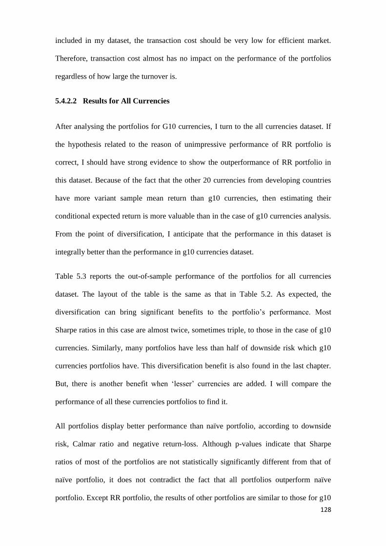
128

included in my dataset, the transaction cost should be very low for efficient market.

Therefore, transaction cost almost has no impact on the performance of the portfolios

regardless of how large the turnover is.

5.4.2.2 Results for All Currencies

After analysing the portfolios for G10 currencies, I turn to the all currencies dataset. If

the hypothesis related to the reason of unimpressive performance of RR portfolio is

correct, I should have strong evidence to show the outperformance of RR portfolio in

this dataset. Because of the fact that the other 20 currencies from developing countries

have more variant sample mean return than g10 currencies, then estimating their

conditional expected return is more valuable than in the case of g10 currencies analysis.

From the point of diversification, I anticipate that the performance in this dataset is

integrally better than the performance in g10 currencies dataset.

Table 5.3 reports the out-of-sample performance of the portfolios for all currencies

dataset. The layout of the table is the same as that in Table 5.2. As expected, the

diversification can bring significant benefits to the portfolio’s performance. Most

Sharpe ratios in this case are almost twice, sometimes triple, to those in the case of g10

currencies. Similarly, many portfolios have less than half of downside risk which g10

currencies portfolios have. This diversification benefit is also found in the last chapter.

But, there is another benefit when ‘lesser’ currencies are added. I will compare the

performance of all these currencies portfolios to find it.

All portfolios display better performance than naïve portfolio, according to downside

risk, Calmar ratio and negative return-loss. Although p-values indicate that Sharpe

ratios of most of the portfolios are not statistically significantly different from that of

naïve portfolio, it does not contradict the fact that all portfolios outperform naïve

portfolio. Except RR portfolio, the results of other portfolios are similar to those for g10

129

Table 5.3 Performance of the portfolios for all currencies


estimation window is 5 years. The database includes 29 currencies induced in chapter three. In the first three columns of table, the ‘1/N’ refers to naïve portfolio, which is equally-

weighted. The ‘Min’ refers to minimum-variance portfolio, and the ‘ERC’ refers to equally weighted risk contribution portfolio. I also report the performance of optimal constrained

portfolio referred as ‘OC’, and volatility timing portfolio referred as ‘VT’ and reward-to-risk portfolio referred as ‘RR’ in panel A and panel B. The number in the bracket followed by

‘VT’ and ‘RR’ is tuning parameter applied in those strategies; I choose this parameter as 1, 2 and 4. In panel A, the conditional expected moments are estimated by simple moving

average (sma). In panel B, I use exponentially weighted moving average to estimate conditional expected moments. The first part shows results from before transaction cost analysis, so I

tagged them with ‘results before transaction cost’. The second part shows results from after transaction cost analysis, so I tagged them with ‘results after transaction cost’. In both parts, I

apply same evaluation methods. For these methods, ‘SR’ refers to Sharpe ratio, ‘vs 1/N’ means that optimal portfolio compare with naïve portfolio. In this category, there are two

comparisons; one is called ‘p-val’, which is the p-value of difference between the Sharpe ratio of each strategy from that of the 1/N, another one is called ‘re-loss’ refer to return-loss.

‘CEQ’ means certainty-equivalent return with risk aversion of 5. ‘VaR’ and ‘CVaR’ mean Value at risk and conditional value at risk, which both are computed at possibility of 95% with

historical sample approach. I report two evaluation indices relevant to drawdown. One is maximum drawdown referred as ‘Maximum’, another one is Calmar ratio referred as ‘CR’.

Except VaR, CVaR and maximum drawdown, the results of all other indices are annualised. In addition, I report turnover only in the part of no transaction cost.


SR vs 1/n


Turnover SR vs 1/n


p-val re-loss Maximum CR p-val re-loss Maximum CR

1/N 0.82 1.00 0.00% 4.70% 1.67% 2.30% 21.74% 0.28 0.01 0.81 1.00 0.00% 4.62% 1.67% 2.30% 21.78% 0.27

Min 0.98 0.34 -0.41% 2.33% 0.55% 0.75% 6.82% 0.37 0.05 0.91 0.52 -0.26% 2.14% 0.56% 0.76% 6.98% 0.33

ERC 1.06 0.17 -1.13% 4.47% 1.04% 1.43% 14.47% 0.35 0.01 1.05 0.17 -1.12% 4.42% 1.05% 1.43% 14.52% 0.34

Panel A: Simple moving average (SMA)

OC 0.81 0.97 0.02% 2.45% 0.70% 1.00% 8.12% 0.34 0.14 0.70 0.36 0.38% 2.05% 0.72% 1.02% 8.26% 0.28

VT(1) 0.91 0.56 -0.37% 3.44% 0.96% 1.30% 13.84% 0.28 0.01 0.89 0.59 -0.34% 3.36% 0.96% 1.30% 13.89% 0.28

VT(2) 0.94 0.45 -0.36% 2.58% 0.67% 0.88% 8.46% 0.33 0.02 0.91 0.50 -0.31% 2.49% 0.67% 0.88% 8.47% 0.32

VT(4) 1.06 0.18 -0.71% 2.88% 0.65% 0.88% 10.21% 0.30 0.02 1.04 0.20 -0.67% 2.81% 0.65% 0.88% 10.21% 0.30

RR(1) 0.90 0.61 -0.35% 3.65% 1.05% 1.44% 13.58% 0.31 0.04 0.86 0.73 -0.23% 3.48% 1.06% 1.45% 13.77% 0.29

RR(2) 1.15 0.09 -1.02% 3.32% 0.70% 0.91% 8.75% 0.41 0.04 1.11 0.11 -0.92% 3.18% 0.70% 0.92% 8.82% 0.39

RR(4) 0.97 0.38 -0.45% 2.72% 0.70% 0.93% 10.22% 0.29 0.03 0.94 0.44 -0.38% 2.62% 0.70% 0.94% 10.23% 0.28

Panel B: Exponentially Weighted Moving Average (EWMA)

OC 0.83 0.96 -0.02% 2.31% 0.58% 0.89% 8.22% 0.31 0.25 0.55 0.02 0.79% 1.47% 0.60% 0.93% 11.40% 0.15

VT(1) 0.95 0.41 -0.52% 3.49% 0.90% 1.25% 13.03% 0.30 0.01 0.93 0.44 -0.48% 3.40% 0.90% 1.25% 13.10% 0.29

VT(2) 1.09 0.15 -0.75% 2.88% 0.64% 0.82% 8.07% 0.38 0.02 1.05 0.17 -0.68% 2.76% 0.64% 0.83% 8.09% 0.37

VT(4) 1.12 0.12 -0.86% 3.00% 0.63% 0.84% 10.18% 0.32 0.02 1.09 0.13 -0.80% 2.89% 0.63% 0.85% 10.18% 0.30

RR(1) 1.03 0.23 -0.94% 4.16% 1.03% 1.44% 12.33% 0.38 0.05 0.98 0.30 -0.77% 3.95% 1.03% 1.45% 12.49% 0.36

RR(2) 1.38 0.02 -1.76% 4.12% 0.69% 0.92% 6.56% 0.67 0.05 1.32 0.02 -1.61% 3.93% 0.69% 0.93% 6.76% 0.62

RR(4) 1.33 0.02 -1.54% 3.80% 0.69% 0.90% 8.93% 0.45 0.05 1.27 0.03 -1.40% 3.63% 0.69% 0.91% 9.19% 0.42

130

currencies dataset. OC and volatility timing portfolio can beat naïve portfolio but

minimum variance portfolio. But, OC portfolio consistently outperforms all volatility

timing (VT) portfolios. If 2 and 4 , the Value at risk and conditional Value at

risk of VT portfolio are less than those of OC portfolio, while their Sharpe ratios are

also higher than OC portfolios. Comparing Panel B to Panel A of Table 5.3, the benefit

of using EWMA rather than SMA also can be found as in the case of g10 currencies.

It is worth noting that the performance of RR portfolios change completely when I

consider all currencies dataset, and it is compelling. With 2 , RR portfolio has the

biggest Sharpe ratio and Calmar ratio. Furthermore, if estimation method of EWMA is

used, the Sharpe ratio of this RR portfolio can be considered to be statistically

significantly different from Sharpe ratio of naïve portfolio according to p-value, and its

maximum drawdown is less than the minimum variance portfolio’s. Although other

downside risks of RR portfolios is not less than the minimum variance portfolio and

some VT portfolios, this slight difference cannot reject its outstanding Sharpe ratio and

Calmar ratio. Similarly, mentioned in preceding paragraphs, impressive performance of

RR portfolios can support that the hypothesis for this thesis is correct.

The conclusion regarding turnover and transaction cost partly differs from the results

obtained for G10 currencies analysis. Firstly, unlike the results based on G10

currencies dataset, turnover of RR portfolios remain a low level. This can be explained

by more efficient RR portfolio in this case than in the case of G10 currencies. The only

portfolio with relatively high level of turnover is OC portfolio. For example, turnover of

OC portfolio with EWMA is 0.25 while the highest turnover during all other portfolios

is 0.5. Secondly, transaction cost, indeed, affects performance of OC portfolio. After

taking transaction cost, positive return-loss indicates that Sharpe ratio of OC portfolio

with EWMA is lower than that of naïve portfolio, and p-value shows that this difference

131

is no longer statistically insignificant. Moreover, its Calmar ratio is reduced to half of

what I get before taking transaction cost. The market of currencies from developing

countries is not as efficient as the market of g10 currencies. This inefficient market

leads to a large gap between bid and ask price, and then large transaction cost. Due to

low level of turnover, the performance of other portfolios seems to be not affected by

transaction cost. So, the high level of turnover and large transaction cost of some

currencies lead to this dramatic drop of performance of OC portfolio.

5.4.3 Robustness Check for Different Lengths of Estimation

Windows

As in chapter four, I conduct robustness analysis by changing the lengths of estimation

windows. However, unlike what was done in chapter four, it is important to evaluate the

performance of the portfolios in the same period for all cases. It seems to be more

reasonable and comparable when I compare the performance across different lengths of

estimation windows. So, the period used to evaluate the performance of the portfolios

here is the same as the period used to evaluate them in the main analysis with 5 years

estimation window. This is more convincing to support validate the conclusions reached

from the main results.

5.4.3.1 Results for 1 year Estimation Window

The results of analysis related to estimating conditional expected moments in 1 year

window are documented in Table 5.4. Generally speaking, this robustness analysis can

almost support the conclusions reached in the main findings. In particular, with respect

to the G10 currencies dataset, there are four consistent conclusions reached. The first

one is that naïve portfolio cannot outperform other portfolios based on the downside

risk. When rewards are considered to construct timing strategy portfolios, the Sharpe

132



estimation window is 1 year. In the first three columns of table, the ‘1/N’ refers to naïve portfolio, which is equally-weighted. The ‘Min’ refers to minimum-variance portfolio, and the

‘ERC’ refers to equally weighted risk contribution portfolio. I also report the performance of optimal constrained portfolio referred as ‘OC’, and volatility timing portfolio referred as ‘VT’

and reward-to-risk portfolio referred as ‘RR’. The tuning parameter applied in those strategies is 2, e.t 2 . The abbreviation after these portfolios presents the estimation method I used.

‘SMA’ refers to simple moving average, and ‘EWMA’ refers to exponentially weighted moving average. The first part shows results from the case of G10 currencies dataset, so I tagged

them with ‘G10 currencies’. The second part shows results from the case of all currencies dataset, so I tagged them with ‘all currencies’. The results before taking transaction cost are

showed in panel A, while the results after taking transaction cost are showed in panel B. For the evaluation methods, ‘SR’ refers to Sharpe ratio, ‘VS 1/N’ means that optimal portfolio

compare with naïve portfolio. In this category, there are two comparisons; one is called ‘p-val’, which is the p-value of difference between the Sharpe ratio of each strategy from that of

the 1/N, another one is called ‘re-loss’ refer to return-loss. ‘CEQ’ means certainty-equivalent return with risk aversion of 5. ‘VaR’ and ‘CVaR’ means Value at risk and conditional value

at risk, which both are computed at possibility of 95% with historical sample approach. I report two evaluation indices relevant to drawdown. One is maximum drawdown referred as

‘Maximum’, another one is Calmar ratio referred as ‘CR’. Except VaR, CVaR and maximum drawdown, the results of all other indices are annualised. In addition, I report turnover only

in panel A. Although estimation window I used is 1 year, the period I used to evaluate the performance is same as in main results analysis.




1/N 0.58 1.00 0.00% 3.25% 1.98% 2.71% 23.94% 0.23 0.01 0.82 1.00 0.00% 4.70% 1.67% 2.30% 21.74% 0.28 0.01

Min 0.58 0.98 -0.02% 3.00% 1.60% 2.22% 14.06% 0.32 0.27 1.49 0.01 -1.81% 3.86% 0.47% 0.81% 4.71% 0.86 0.36

ERC 0.62 0.64 -0.36% 3.50% 1.85% 2.41% 20.59% 0.26 0.02 0.98 0.32 -0.77% 4.15% 1.04% 1.54% 15.40% 0.31 0.10

OC-SMA 0.46 0.14 0.98% 2.11% 1.77% 2.38% 17.47% 0.22 0.42 1.03 0.24 -0.85% 3.73% 0.82% 1.38% 12.64% 0.33 0.63

VT-SMA 0.53 0.55 0.38% 2.71% 1.84% 2.40% 21.53% 0.21 0.05 1.39 0.01 -1.64% 3.79% 0.44% 0.74% 7.46% 0.54 0.06

RR-SMA 0.47 0.15 1.08% 2.17% 2.17% 2.86% 14.28% 0.31 0.19 1.98 0.00 -3.24% 5.33% 0.51% 0.91% 7.72% 0.72 0.09

OC-

EWMA 0.51 0.45 0.56% 2.55% 1.78% 2.40% 16.54% 0.26 0.54 1.14 0.10 -4.60% 11.24% 3.23% 4.54% 25.01% 0.66 0.04

VT-

EWMA 0.57 0.92 0.07% 3.00% 1.82% 2.30% 19.08% 0.24 0.06 1.52 0.01 -1.89% 3.92% 0.41% 0.73% 6.63% 0.62 0.07

RR-

EWMA 0.48 0.22 0.94% 2.30% 2.15% 2.90% 16.09% 0.28 0.25 1.89 0.00 -3.67% 6.20% 0.55% 0.98% 5.36% 1.21 0.12




1/N 0.58 1.00 0.00% 3.23% 1.99% 2.71% 23.95% 0.23 0.81 1.00 0.00% 4.62% 1.67% 2.30% 21.78% 0.27

Min 0.54 0.67 0.29% 2.68% 1.61% 2.24% 14.20% 0.29 1.05 0.19 -0.63% 2.61% 0.51% 0.86% 5.80% 0.48

ERC 0.62 0.61 -0.39% 3.51% 1.86% 2.41% 20.62% 0.26 0.88 0.65 -0.32% 3.65% 1.04% 1.55% 15.55% 0.27

OC-SMA 0.41 0.02 1.44% 1.65% 1.78% 2.40% 17.74% 0.19 0.48 0.00 1.32% 1.56% 0.89% 1.50% 16.35% 0.12

VT-SMA 0.53 0.57 0.37% 2.71% 1.84% 2.41% 21.59% 0.20 1.36 0.02 -1.46% 3.44% 0.46% 0.76% 7.62% 0.47

RR-SMA 0.44 0.07 1.31% 1.93% 2.18% 2.87% 14.50% 0.29 1.84 0.00 -2.83% 4.87% 0.53% 0.94% 7.98% 0.63

OC-

EWMA 0.43 0.05 1.25% 1.85% 1.87% 2.44% 16.88% 0.21 1.13 0.10 -4.57% 11.05% 3.23% 4.56% 25.07% 0.65

VT-

EWMA 0.57 0.90 0.08% 2.97% 1.82% 2.30% 19.17% 0.24 1.47 0.01 -1.65% 3.52% 0.42% 0.75% 6.88% 0.53

RR-

EWMA 0.44 0.07 1.31% 1.92% 2.16% 2.92% 16.68% 0.25 1.70 0.00 -3.09% 5.60% 0.57% 1.04% 5.98% 0.99

133

ratio is decreased, and VaR and CVaR are increased. The second one shows that the

results do not support RR portfolios. Moreover, according to the changes of most

evaluation indices from estimation method of SMA to EWMA, the third one is that

EWMA can improve the performance of portfolios. After comparing results before

taking transaction cost to those after taking transaction cost, the last one supports the

fact that transaction cost does not affect the performance significantly regardless of

turnover value. In addition, there are some inconsistent points when I make these

consistent conclusions. For example, the question about whether OC portfolio

outperforms timing strategies portfolio is ambiguous, and maximum drawdown is

decreased after taking account of rewards in timing strategy. VaR and CVaR of RR

portfolio is higher than those of naïve portfolios. But, because these inconsistent points

are inconspicuous, the conclusions reached cannot be totally rejected.

In response to the all currencies dataset, the results are robust to the conclusions from

main results analysis. Firstly, comparing to results of G10 currencies analysis, adding

‘lesser’ currencies delivers huge diversification benefits, except that downside risk of

OC portfolio with estimation method of EWMA (referred as OC-EWMA portfolio) is

increased, but its Sharpe ratio and Calmar ratio is raised significantly as well. Secondly,

in addition to that downside risk of OC-EWMA portfolio is higher than that of naïve

portfolio, all other portfolios consistently outperform naïve portfolio in all terms of

evaluation. Moreover, timing strategy portfolios have better performance than OC

portfolio. Thirdly, although the advantage of using EWMA is not expressed consistently,

most of the terms of evaluation index can also display improvement from application of

estimation method of EWMA. Finally, unlike analysis related to G10 currencies dataset,

RR portfolio has outstanding performance, which can be considered to be better than

the performance of minimum variance portfolio. In addition, turnover of RR portfolio

remains at low level, which is just half of the original to G10 currencies analysis. With

134

high level of turnover, e.g. OC portfolio, the transaction cost has obvious impact on the

performance. For example, after taking transaction cost, I find that the drop of Sharpe

ratio and Calmar ratio of OC portfolio with turnover of 0.63 is significant. These

conclusions are totally consistent with analysis for the main results using 5 years

estimation window.

5.4.3.2 Results for 3 years Estimation Window

According to Table 5.5, which documents the results related to 3 years estimation

window, I find that the conclusions made in the main results analysis are also tenable in

this case. Firstly, making comparison between the left and the right side of table, I can

easily find that ‘lesser’ currencies can bring the portfolio lots of diversification benefits.

This has already been proven in chapter four, and confirmed in the previous discussion

in this chapter. I will not mention this conclusion again in the following robustness

check analysis, which also can show this benefit.

Next, OC portfolio displays a better performance than naïve portfolio and other timing

strategies portfolio in the case of G10 currencies dataset, however, this portfolio can

only beat naïve portfolio but not timing strategy portfolios in the case of all currencies

dataset. Based on the case of G10 currencies dataset, OC portfolio has higher Sharp

ratio, as well as Calmar ratio, and less downside risk than volatility timing and reward-

to-risk portfolios. But, as far as all currencies dataset is concerned, I cannot generally

say that all evaluation indices indicate outperformance of OC portfolio against timing

strategy portfolios, because some indices do not agree to that.

For example VaR and CVaR of volatility timing portfolio is less than OC portfolio.

Even, RR portfolio with an estimation method of EWMA (referred as RR-EWMA

portfolio) has outstanding Sharpe ratio and Calmar ratio, while its downside risk also

135



estimation window is 3 years. In the first three columns of table, the ‘1/N’ refers to naïve portfolio, which is equally-weighted. The ‘Min’ refers to minimum-variance portfolio, and the





showed in panel A, while the results after taking transaction cost are showed in panel B. For the evaluation methods, ‘SR’ refers to Sharpe ratio. There are two comparisons; one is called

‘p-val’, which is the p-value of difference between the Sharpe ratio of each strategy from that of the 1/N, another one is called ‘re-loss’ refer to return-loss. ‘CEQ’ means certainty-

equivalent return with risk aversion of 5. ‘VaR’ and ‘CVaR’ means Value at risk and conditional value at risk, which both are computed at possibility of 95% with historical sample

approach. I report two evaluation indices relevant to drawdown. One is maximum drawdown referred as ‘Maximum’, another one is Calmar ratio referred as ‘CR’. Except VaR, CVaR

and maximum drawdown, the results of all other indices are annualised. In addition, I report turnover only in panel A. Although estimation window I used is 3 year, the period I used to

evaluate the performance is same as in main results analysis.




1/N 0.58 1.00 0.00% 3.25% 1.98% 2.71% 23.94% 0.23 0.01 0.82 1.00 0.00% 4.70% 1.67% 2.30% 21.74% 0.28 0.01

Min 0.74 0.16 -1.15% 4.05% 1.55% 2.05% 12.60% 0.43 0.08 1.59 0.00 -1.72% 3.42% 0.43% 0.60% 5.23% 0.68 0.08

ERC 0.63 0.62 -0.37% 3.47% 1.80% 2.36% 20.91% 0.25 0.01 0.99 0.30 -0.83% 4.25% 1.06% 1.49% 15.19% 0.32 0.03

OC-SMA 0.65 0.47 -0.57% 3.58% 1.60% 2.15% 14.07% 0.36 0.15 1.53 0.01 -2.00% 4.10% 0.55% 0.75% 5.65% 0.76 0.21

VT-SMA 0.54 0.63 0.32% 2.78% 1.80% 2.36% 21.16% 0.21 0.02 1.48 0.01 -1.63% 3.52% 0.54% 0.72% 6.91% 0.53 0.02

RR-SMA 0.46 0.09 1.13% 2.08% 1.97% 2.78% 28.70% 0.14 0.11 1.56 0.00 -2.05% 4.13% 0.58% 0.79% 7.30% 0.59 0.05

OC-EWMA 0.72 0.21 -1.10% 4.12% 1.55% 2.13% 14.15% 0.40 0.21 1.26 0.04 -1.27% 3.44% 0.54% 0.86% 7.41% 0.49 0.26

VT-EWMA 0.57 0.85 0.13% 2.96% 1.80% 2.33% 20.51% 0.23 0.02 1.48 0.01 -1.64% 3.52% 0.53% 0.72% 6.94% 0.53 0.03

RR-EWMA 0.54 0.65 0.37% 2.85% 2.11% 2.82% 16.34% 0.30 0.13 1.84 0.00 -2.82% 4.89% 0.58% 0.83% 5.18% 0.98 0.06




1/N 0.58 1.00 0.00% 3.23% 1.99% 2.71% 23.95% 0.23 0.81 1.00 0.00% 4.62% 1.67% 2.30% 21.78% 0.27

Min 0.74 0.16 -1.15% 4.05% 1.55% 2.06% 12.81% 0.42 1.46 0.01 -1.45% 3.12% 0.44% 0.61% 5.54% 0.59

ERC 0.63 0.58 -0.42% 3.51% 1.80% 2.36% 20.93% 0.25 0.96 0.33 -0.75% 4.12% 1.07% 1.50% 15.33% 0.31

OC-SMA 0.65 0.51 -0.51% 3.51% 1.61% 2.16% 14.38% 0.35 1.29 0.03 -1.35% 3.44% 0.59% 0.78% 6.19% 0.59

VT-SMA 0.55 0.70 0.25% 2.83% 1.80% 2.37% 21.19% 0.22 1.43 0.01 -1.55% 3.41% 0.55% 0.72% 6.95% 0.51

RR-SMA 0.44 0.05 1.27% 1.93% 1.97% 2.79% 28.91% 0.14 1.49 0.01 -1.88% 3.94% 0.59% 0.80% 7.60% 0.54

OC-EWMA 0.70 0.27 -0.95% 3.96% 1.55% 2.15% 14.33% 0.38 0.96 0.38 -0.44% 2.60% 0.55% 0.91% 10.45% 0.27

VT-EWMA 0.57 0.91 0.08% 2.99% 1.80% 2.34% 20.56% 0.23 1.44 0.01 -1.53% 3.36% 0.53% 0.73% 6.98% 0.50

RR-EWMA 0.52 0.50 0.53% 2.67% 2.12% 2.83% 16.46% 0.29 1.75 0.00 -2.59% 4.64% 0.59% 0.85% 5.32% 0.91

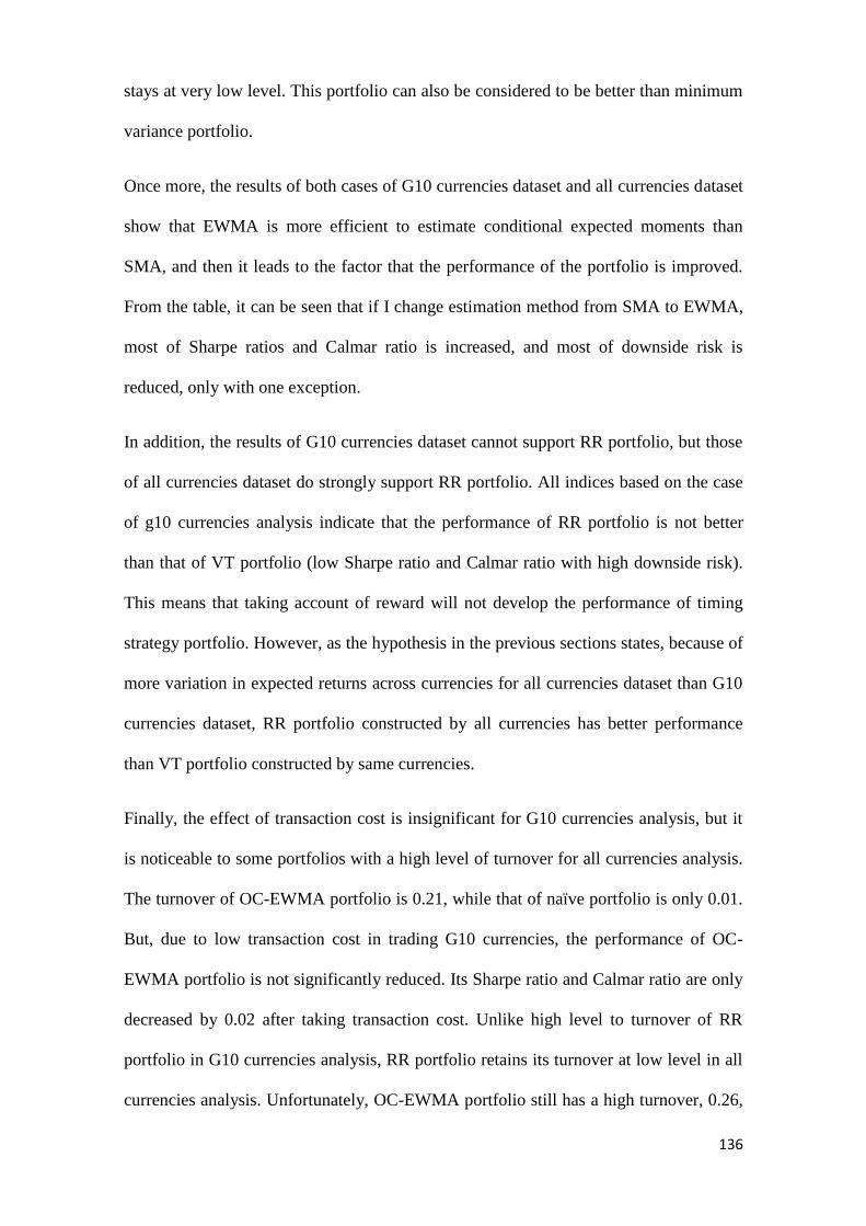
136

stays at very low level. This portfolio can also be considered to be better than minimum

variance portfolio.

Once more, the results of both cases of G10 currencies dataset and all currencies dataset

show that EWMA is more efficient to estimate conditional expected moments than

SMA, and then it leads to the factor that the performance of the portfolio is improved.

From the table, it can be seen that if I change estimation method from SMA to EWMA,

most of Sharpe ratios and Calmar ratio is increased, and most of downside risk is

reduced, only with one exception.

In addition, the results of G10 currencies dataset cannot support RR portfolio, but those

of all currencies dataset do strongly support RR portfolio. All indices based on the case

of g10 currencies analysis indicate that the performance of RR portfolio is not better

than that of VT portfolio (low Sharpe ratio and Calmar ratio with high downside risk).

This means that taking account of reward will not develop the performance of timing

strategy portfolio. However, as the hypothesis in the previous sections states, because of

more variation in expected returns across currencies for all currencies dataset than G10

currencies dataset, RR portfolio constructed by all currencies has better performance

than VT portfolio constructed by same currencies.

Finally, the effect of transaction cost is insignificant for G10 currencies analysis, but it

is noticeable to some portfolios with a high level of turnover for all currencies analysis.

The turnover of OC-EWMA portfolio is 0.21, while that of naïve portfolio is only 0.01.

But, due to low transaction cost in trading G10 currencies, the performance of OC-

EWMA portfolio is not significantly reduced. Its Sharpe ratio and Calmar ratio are only

decreased by 0.02 after taking transaction cost. Unlike high level to turnover of RR

portfolio in G10 currencies analysis, RR portfolio retains its turnover at low level in all

currencies analysis. Unfortunately, OC-EWMA portfolio still has a high turnover, 0.26,

137

in an analysis related to all currencies dataset. Moreover, due to subtraction of

transaction cost from portfolio return, the Sharpe ratio is reduced by 0.3, from 1.26 to

0.96. So, the effect of transaction cost is considered to be significant to all currencies

analysis, while it is insignificant to G10 currencies analysis.

5.4.3.3 Results for 10 years Estimation Window

In this subsection, I turn to focus on 10 years estimation window, which is longer than

what I use in the main results analysis. However, due to longer estimation window, the

evaluation period will be shortened. Consequently, I cannot use the same evaluation

period as in the main results analysis. I therefore, can only report the evaluation results

for the period of the last 5 years. Although evaluating the performance with different

period lengths is not very fair and suitable to the comparison, it is still valuable in some

ways to analyse the results of this case.

The evaluation results related to 10 years estimation window are documented in Table

5.6, which shows some inconsistences with the main results analysis. According to p-

value of zero and positive return-loss, naïve portfolio has better Sharpe ratio than OC

and timing strategy portfolios have with statistically significant differences for both

cases of G10 and all currencies datasets. In contrast, downside risks of those portfolios,

except RR portfolio in the case of G10 currencies dataset, are less than naïve portfolios.

However, Calmar ratios support the performance of Sharpe ratio. So, if the risk is the

only major concern of an investor, investor, the naïve portfolio does not outperform

others, but if an investor also has an interest about return, naïve portfolio should be the

best choice, because the difference of downside risk is not large. The same situation

happens when I compare the performances of OC portfolio and timing strategy

portfolios.

138












and maximum drawdown, the results of all other indices are annualised. In addition, I report turnover only in panel A. because the estimation window I used is 10 year, I can only report

the evaluation results for the period of the last 5 years.




1/N 0.29 1.00 0.00% 0.17% 2.52% 3.16% 23.94% 0.14 0.01 0.34 1.00 0.00% 1.02% 2.06% 2.80% 21.74% 0.15 0.01

Min 0.02 0.00 2.24% -1.50% 1.68% 2.25% 18.90% 0.01 0.03 0.17 0.01 0.68% 0.27% 1.03% 1.30% 12.49% 0.05 0.04

ERC 0.29 0.92 0.05% 0.38% 2.17% 2.86% 22.00% 0.13 0.01 0.41 0.46 -0.43% 1.60% 1.43% 2.01% 17.21% 0.16 0.01

OC-SMA 0.04 0.00 2.35% -1.77% 2.00% 2.55% 20.27% 0.02 0.09 0.04 0.00 1.41% -0.37% 1.10% 1.54% 15.60% 0.01 0.08

VT-SMA 0.14 0.00 1.53% -1.11% 2.19% 2.92% 22.70% 0.06 0.01 0.21 0.01 0.72% 0.40% 1.40% 1.63% 16.74% 0.07 0.01

RR-SMA 0.10 0.00 2.71% -3.38% 2.96% 4.18% 29.67% 0.04 0.05 0.13 0.00 1.52% -0.36% 1.65% 2.29% 23.61% 0.04 0.05

OC-EWMA 0.08 0.00 1.75% -1.05% 1.81% 2.33% 20.50% 0.03 0.11 -0.10 0.00 1.56% -0.67% 0.85% 1.17% 12.55% -0.03 0.12

VT-EWMA 0.17 0.00 1.19% -0.71% 2.16% 2.80% 21.72% 0.08 0.01 0.21 0.01 0.63% 0.43% 1.15% 1.45% 15.28% 0.07 0.01

RR-EWMA -0.20 0.00 6.20% -6.43% 3.04% 4.03% 36.89% -0.07 0.11 0.03 0.00 1.75% -0.63% 1.25% 1.89% 19.93% 0.01 0.06




1/N 0.29 1.00 0.00% 0.14% 2.52% 3.17% 23.95% 0.14 0.33 1.00 0.00% 0.89% 2.07% 2.82% 21.78% 0.14

Min 0.02 0.00 2.09% -1.38% 1.69% 2.26% 18.98% 0.01 0.13 0.00 0.79% 0.12% 1.04% 1.31% 12.66% 0.04

ERC 0.29 0.98 -0.02% 0.42% 2.18% 2.87% 22.01% 0.13 0.39 0.44 -0.44% 1.51% 1.43% 2.02% 17.26% 0.15

OC-rolling 0.04 0.00 2.27% -1.71% 2.01% 2.57% 20.42% 0.02 -0.02 0.00 1.59% -0.61% 1.11% 1.55% 15.93% 0.00

VT-rolling 0.14 0.00 1.46% -1.07% 2.20% 2.94% 22.71% 0.06 0.19 0.01 0.75% 0.30% 1.41% 1.63% 16.79% 0.06

RR-rolling 0.09 0.00 2.81% -3.52% 2.97% 4.21% 29.76% 0.04 0.10 0.00 1.67% -0.61% 1.66% 2.31% 23.81% 0.03

OC-EWMA 0.08 0.00 1.66% -0.98% 1.83% 2.34% 20.78% 0.03 -0.18 0.00 1.82% -0.97% 0.86% 1.19% 13.03% -0.05

VT-EWMA 0.17 0.00 1.10% -0.64% 2.17% 2.81% 21.75% 0.08 0.19 0.01 0.65% 0.35% 1.15% 1.46% 15.35% 0.06

RR-EWMA -0.22 0.00 6.37% -6.63% 3.06% 4.06% 37.14% -0.07 -0.03 0.00 1.98% -0.93% 1.27% 1.91% 20.33% -0.01

139

Again, taking return into timing strategy portfolio cannot improve its performance in the

case of G10 currencies dataset. However, in the case of all currencies dataset, this is still

useless in terms of making the performance better. For both cases, the Sharpe and

Calmar ratios of VT portfolios are better than those of RR portfolio, while former

downsides are consistently higher than the latter. In addition, only OC and VT

portfolios for G10 currencies analysis have improved performance when EWMA is

applied instead of SMA to estimate moments. But, RR portfolio has worse performance

than before. Moreover, for all currencies analysis, only decreasing downside risk can

confirm this improvement, but not Sharpe and Calmar ratio. So, unlike previous

analyses, the advantage of EWMA is ambiguous, here. If risk is considered as the only

evaluation to the performance, EWMA can be concluded roughly to improve the

performance of portfolios.

As far as results after taking transaction cost are concerned, the reduction of the

performance is not significant due to transaction cost for both cases of G10 and all

currencies datasets. After comparing Panel B to Panel A of Table 5.6, I find that there is

almost unchanged to all evaluation indices for G10 currencies analysis. As explained,

the reasons for this tiny effect of transaction cost are small transaction costs and low

turnover. Although transaction cost is relatively large for the case of all currencies

dataset, low turnover also leads to the factor that the performance of the portfolios is not

affected significantly.

In summary, the results related to 1 year and 3 years estimation windows can confirm

the conclusions obtained from the main results analysis (5 years estimation window).

Although conclusions from results of 10 years estimation window are not consistent

mostly, this analysis just evaluates the performance of the portfolios in the last 5 year

period, which is different to the evaluation period of the main results analysis. Moreover,

140

in some ways, analysis of 10 years estimation window also has robustness to my main

results analysis.

5.4.4 Robustness Check for Investor Perspectives from Different

Countries

As in chapter four, I also conduct robustness check analysis in a different direction,

which considers perspectives of investors from other countries. I will still use 5 years

estimation window, and the countries include the United Kingdom, Japan, and euro

zone as whole.

5.4.4.1 United Kingdom (UK) Investor

Results related to the perspective of investors from United Kingdom (UK) are

documented in Table 5.7, and these results only partly support the conclusions of the

main results analysis. According to this table, all positive return-loss means that Sharpe

ratio of naïve portfolio is higher than that of other portfolios for both cases of G10 and

all currencies datasets, and p-value indicates that most of the differences between

Sharpe ratios are statistically significantly different. And, other evaluation indices also

confirm the best performance of naïve portfolio. Furthermore, all evaluation indices

display that volatility timing portfolio has better performance than OC portfolio. Based

on Sharpe ratio and Calmar ratio, timing strategy portfolios and OC portfolio

outperform minimum variance portfolio.

141


This table documents the evaluation of performance of each optimal portfolio strategy for UK investor’s perspective. This means that I treated British pound as the based currency. The










and maximum drawdown, the results of all other indices are annualised. In addition, I report turnover only in panel A.




1/N 0.58 1.00 0.00% 2.80% 1.31% 1.70% 14.95% 0.26 0.01 0.67 1.00 0.00% 3.55% 1.47% 1.88% 10.21% 0.47 0.01

Min 0.25 0.00 2.36% 0.52% 1.35% 1.87% 23.28% 0.08 0.04 0.26 0.00 3.08% 0.57% 1.34% 2.08% 18.06% 0.11 0.16

ERC 0.55 0.72 0.23% 2.58% 1.31% 1.71% 16.37% 0.23 0.01 0.64 0.74 0.24% 3.24% 1.43% 1.80% 10.56% 0.42 0.01

OC-SMA 0.30 0.00 2.03% 0.85% 1.41% 1.91% 21.49% 0.10 0.07 0.35 0.00 2.52% 1.22% 1.46% 2.26% 15.14% 0.18 0.21

VT-SMA 0.44 0.05 1.02% 1.83% 1.31% 1.79% 18.08% 0.17 0.01 0.51 0.06 1.11% 2.34% 1.39% 1.80% 12.23% 0.29 0.01

RR-SMA 0.26 0.00 2.65% 0.46% 1.86% 2.51% 16.80% 0.13 0.10 0.56 0.24 0.91% 2.86% 1.55% 2.28% 14.01% 0.32 0.08

OC-EWMA 0.25 0.00 2.31% 0.55% 1.40% 1.89% 22.70% 0.08 0.09 0.33 0.00 2.72% 1.03% 1.47% 2.34% 16.60% 0.16 0.27

VT-EWMA 0.44 0.07 0.98% 1.86% 1.27% 1.79% 18.50% 0.17 0.02 0.50 0.04 1.20% 2.24% 1.40% 1.81% 12.89% 0.26 0.02

RR-EWMA 0.40 0.02 1.57% 1.60% 1.98% 2.55% 15.16% 0.23 0.12 0.57 0.27 0.85% 2.89% 1.67% 2.16% 11.80% 0.37 0.11




1/N 0.58 1.00 0.00% 2.79% 1.31% 1.70% 14.97% 0.26 0.66 1.00 0.00% 3.47% 1.47% 1.88% 10.23% 0.47

Min 0.24 0.00 2.43% 0.44% 1.35% 1.88% 23.40% 0.07 0.21 0.00 3.43% 0.14% 1.35% 2.10% 19.19% 0.08

ERC 0.55 0.72 0.23% 2.57% 1.31% 1.71% 16.39% 0.23 0.63 0.73 0.25% 3.16% 1.43% 1.80% 10.59% 0.41

OC-SMA 0.29 0.00 2.08% 0.79% 1.42% 1.92% 21.69% 0.10 0.29 0.00 2.93% 0.73% 1.49% 2.29% 16.00% 0.14

VT-SMA 0.43 0.05 1.04% 1.80% 1.31% 1.79% 18.10% 0.17 0.50 0.05 1.12% 2.26% 1.39% 1.81% 12.35% 0.28

RR-SMA 0.25 0.00 2.76% 0.33% 1.86% 2.52% 17.18% 0.12 0.53 0.13 1.09% 2.60% 1.56% 2.30% 14.33% 0.29

OC-EWMA 0.24 0.00 2.37% 0.48% 1.41% 1.90% 22.95% 0.07 0.24 0.00 3.30% 0.37% 1.48% 2.37% 17.01% 0.11

VT-EWMA 0.44 0.06 1.00% 1.83% 1.28% 1.80% 18.53% 0.16 0.49 0.03 1.21% 2.16% 1.40% 1.81% 13.02% 0.26

RR-EWMA 0.38 0.01 1.70% 1.46% 1.98% 2.56% 15.29% 0.22 0.52 0.12 1.10% 2.56% 1.68% 2.17% 11.93% 0.34

142

Similar to the main results analysis, taking returns cannot improve the timing strategy

portfolio for G10 currencies analysis, but it helps investors to have better performance

than VT portfolio has if all currencies dataset is considered. In the case of G10

currencies dataset, Sharpe ratio of RR portfolio is smaller than that of VT portfolio,

while RR portfolio has more downside risks, except maximum drawdown, than VT

portfolio has. Although maximum drawdown is less to RR portfolio than VT portfolio,

Calmar ratio indicates that VT portfolio outperforms RR portfolio. However, in the case

of all currencies dataset, Sharpe ratio shows a better performance of RR portfolio than

VT portfolio. Admitting that RR portfolio is riskier than VT portfolio, the difference

between two portfolios’ downside risk is very small. Moreover, RR portfolio has higher

Calmar ratio than VT portfolio has.

The role of using EWMA instead of SMA to estimate conditional expected moments is

not clear here for both G10 and all currencies analysis. In the G10 currencies analysis,

VaR and CVaR of OC and VT portfolios have slight decrease after using EWMA. But,

maximum drawdown of these two portfolios is increased. Moreover, these two

portfolios have lower Sharpe ratio/CEQ and Calmar ratio for estimation method of

EWMA than SMA. Correspondingly, the estimation method of EWMA increases

Sharpe ratio/CEQ and Calmar ratio of RR portfolio. And, maximum drawdown of this

portfolio is lower with EWMA than SMA. But, this portfolio has VaR and CVaR,

which are larger in EWMA than SMA. According to results from all currencies analysis,

a similar situation happens, other than the fact that all downside risks of three portfolios

are raised because of using EWMA.

With respect to transaction costs, the performance of the portfolio with G10 currencies

dataset is not affected significantly. By comparison, in the case of all currencies dataset,

transaction cost, indeed, has impact on the performance of some portfolios. All

143

portfolios in G10 currencies analysis have low level of turnover. Therefore, comparing

the results before to after taking transaction cost, I find that the changes of all evaluation

indices are very slight. However, the turnover of OC portfolio in all currencies analysis

remains at relatively high level. So, after taking transaction cost, this portfolio has a big

drop in Sharpe ratio and Calmar ratio. The reason for this change also includes high

transaction cost for developing countries’ currencies. Although the impact is not

ignorable, the ranking of the performance is unchanged.

5.4.4.2 Japanese (JP) Investor

According to Table 5.8, which reports the results of analysis related to perspective of

investors from Japan, I find that, like the UK investor analysis, some conclusions are

not consistent with the conclusion of the main results analysis. Firstly, based on Sharpe

ratio and Calmar ratio in both cases of G10 and all currencies datasets, I can conclude

that other portfolios cannot beat naïve portfolio, although some downside risk of other

portfolios is less than that of naïve portfolio. Furthermore, these two ratios of OC

portfolio are lower than those of VT portfolios. With lower maximum drawdown, I

roughly conclude that VT portfolio has better performance than OC portfolio.

Secondly, unlike results related to main results analysis, I find evidence not only in all

currencies analysis to support RR portfolio, but also in G10 currencies analysis. For

both cases, Sharpe ratio and Calmar ratio are increased due to taking account of returns

in timing strategy. However, the downside risk in the case of G10 currencies dataset is

also raised to a large extent. It can therefore be said that I find evidence to prove the

advantage of use of return in the case of G10 currencies dataset. But, I cannot conclude

that RR portfolio has better performance than VT portfolio.

144


This table documents the evaluation of performance of each optimal portfolio strategy for Japanese investor’s perspective. This means that I treated Japanese yen as the based currency.

The estimation window is 5 years. In the first three columns of table, the ‘1/N’ refers to naïve portfolio, which is equally-weighted. The ‘Min’ refers to minimum-variance portfolio, and

the ‘ERC’ refers to equally weighted risk contribution portfolio. I also report the performance of optimal constrained portfolio referred as ‘OC’, and volatility timing portfolio referred as

‘VT’ and reward-to-risk portfolio referred as ‘RR’. The tuning parameter applied in those strategies is 2, e.t 2 . The abbreviation after these portfolios presents the estimation method I

used. ‘SMA’ refers to simple moving average, and ‘EWMA’ refers to exponentially weighted moving average. The first part shows results from the case of G10 currencies dataset, so I

tagged them with ‘G10 currencies’. The second part shows results from the case of all currencies dataset, so I tagged them with ‘all currencies’. The results before taking transaction cost

are showed in panel A, while the results after taking transaction cost are showed in panel B. For the evaluation methods, ‘SR’ refers to Sharpe ratio. There are two comparisons; one is

called ‘p-val’, which is the p-value of difference between the Sharpe ratio of each strategy from that of the 1/N, another one is called ‘re-loss’ refer to return-loss. ‘CEQ’ means certainty-







1/N 0.25 1.00 0.00% -0.71% 2.96% 4.24% 34.99% 0.09 0.01 0.35 1.00 0.00% 0.62% 2.70% 4.01% 32.77% 0.12 0.01

Min 0.02 0.00 2.08% -1.81% 1.94% 2.61% 30.85% 0.01 0.07 0.09 0.00 2.30% -1.21% 1.86% 2.64% 30.31% 0.03 0.21

ERC 0.23 0.46 0.25% -0.71% 2.77% 4.00% 33.64% 0.08 0.01 0.32 0.49 0.31% 0.40% 2.55% 3.85% 31.83% 0.11 0.01

OC-SMA 0.06 0.00 2.02% -2.03% 2.12% 3.34% 35.20% 0.02 0.16 0.18 0.00 1.53% -0.49% 2.16% 2.79% 33.43% 0.05 0.27

VT-SMA 0.18 0.00 0.77% -0.84% 2.40% 3.57% 32.05% 0.06 0.01 0.21 0.00 1.33% -0.40% 2.28% 3.42% 29.68% 0.07 0.01

RR-SMA 0.24 0.66 0.19% -1.14% 3.15% 4.63% 38.57% 0.08 0.10 0.24 0.00 1.25% -0.60% 2.58% 3.92% 35.88% 0.08 0.08

OC-EWMA 0.16 0.07 0.89% -0.84% 2.06% 3.02% 28.15% 0.06 0.22 0.24 0.04 0.97% 0.10% 1.97% 2.64% 31.08% 0.07 0.33

VT-EWMA 0.18 0.00 0.75% -0.75% 2.40% 3.43% 31.32% 0.06 0.01 0.20 0.00 1.42% -0.46% 2.24% 3.37% 29.28% 0.07 0.01

RR-EWMA 0.20 0.11 0.73% -1.47% 3.03% 4.52% 40.49% 0.06 0.13 0.30 0.27 0.54% 0.11% 2.61% 3.99% 34.13% 0.10 0.12




1/N 0.23 1.00 0.00% -0.99% 2.96% 4.24% 35.00% 0.08 0.32 1.00 0.00% 0.30% 2.70% 4.02% 32.79% 0.11

Min -0.01 0.00 2.15% -2.09% 1.94% 2.62% 30.99% 0.00 0.01 0.00 2.76% -1.91% 1.87% 2.67% 31.62% 0.00

ERC 0.21 0.39 0.26% -0.98% 2.77% 4.01% 33.64% 0.07 0.29 0.44 0.32% 0.09% 2.55% 3.86% 31.85% 0.10

OC-SMA 0.02 0.00 2.12% -2.36% 2.13% 3.36% 35.57% 0.01 0.10 0.00 2.06% -1.28% 2.18% 2.82% 34.72% 0.03

VT-SMA 0.16 0.00 0.79% -1.10% 2.41% 3.57% 32.07% 0.05 0.18 0.00 1.36% -0.70% 2.28% 3.43% 29.75% 0.06

RR-SMA 0.21 0.57 0.22% -1.47% 3.15% 4.64% 38.66% 0.07 0.21 0.00 1.28% -0.96% 2.59% 3.94% 36.29% 0.07

OC-EWMA 0.13 0.03 1.02% -1.20% 2.07% 3.03% 28.74% 0.04 0.14 0.00 1.63% -0.82% 1.99% 2.69% 33.14% 0.04

VT-EWMA 0.15 0.00 0.78% -1.01% 2.40% 3.44% 31.36% 0.05 0.17 0.00 1.46% -0.77% 2.24% 3.38% 29.37% 0.06

RR-EWMA 0.17 0.06 0.81% -1.84% 3.04% 4.54% 40.71% 0.05 0.26 0.10 0.71% -0.39% 2.63% 4.02% 35.09% 0.08

145

Finally, estimation method of EWMA can help some portfolios to improve their

performance, but not all of them. For both G10 and all currencies analysis, because all

terms of evaluation have development, using EWMA to replace SMA can improve the

performance of OC and VT portfolios. Moreover, this improvement for OC portfolio is

obvious, while VT portfolio does not have obvious improvement. In contrast, RR

portfolio with SMA has less downside risk than what EWMA has. Furthermore, Sharpe

ratio and Calmar ratio are higher to RR portfolio with SMA than EWMA for G10

currencies analysis. However, as with all currencies analysis, EWMA increases Sharpe

ratio and Calmar ratio of RR portfolio. In addition to previous inconsistent points, the

conclusion about the effect of transaction cost is consistent with the main results

analysis. By comparison with the results before taking transaction cost, results after

transaction cost for the case of G10 currencies dataset display almost unchanged

evaluation indices. This indicates insignificant effect of transaction cost, even if

turnover is high. However, in the case of all currencies dataset, transaction cost is

meaningful to the portfolio with high level of turnover. For example, due to the fact that

OC-EWMA portfolio has high turnover of 0.33, its Sharpe ratio is decreased from 0.24

to 0.14 when I take account of transaction cost.

5.4.4.3 Euro zone (EZ) Investor

The results about analysis related to perspectives of investors who comes from euro

zone countries are documented in Table 5.9. From this table, I can only find evidence to

support some of the conclusions made in the main results analysis. The first evidence is

about adding returns into building of timing strategy portfolio. In the case of G10

currencies dataset, VT portfolio has higher Sharpe ratio and Calmar ratio than RR

portfolio has, while downside risk of VT portfolio is less than that of RR portfolio. This

means that taking account of returns cannot boost the performance of timing strategy

146

portfolio. However, when I consider the case of all currencies dataset, the advantage of

constructing timing strategy portfolio with both volatility and return can be found. As to

all currencies analysis, Sharpe ratio and Calmar ratio of RR portfolio is higher than that

of VT portfolio. Although more downside risk is attributed to RR portfolio than VT

portfolio, the huge improvement on Sharp ratio and Calmar ratio confirms better

performance of RR portfolio than VT portfolio.

The second evidence is related to turnover and effect of transaction cost. As far as G10

currencies dataset is concerned, most portfolios remain with low turnover, and only RR

portfolio has high turnover, 0.14 for SMA and 0.19 for EWMA. With this high level of

turnover, RR portfolio still has almost unchanged performance after taking transaction

cost. So, this means that transaction cost has insignificant effect to the performance

regardless of the level of turnover for the case of G10 currencies dataset. But, as in the

main results analysis, the situation for the case of all currencies dataset is different.

Sharpe ratio and Calmar ratio is dropped hugely for OC portfolio, whose turnover stays

at high level. Therefore, transaction cost can impact on the portfolio with high turnover,

when I consider all currencies analysis.

In addition to supporting evidence, from the results of Table 5.9, I also can find some

inconsistent conclusions with the main results analysis. In the first place, naïve portfolio

can be considered as having the best performance. In G10 currencies analysis, return-

loss indicates that naïve portfolio has higher Sharpe ratio than others have, and p-value

confirms this difference is statistically significant. The highest Calmar ratio of naïve

portfolio also agrees the best portfolio of naïve portfolio. VaR and CVaR of some

portfolios are lower than those of naïve portfolio. But, naïve portfolio has the lowest

maximum drawdown. In all currencies analysis, although p-value indicates no

statistically significant difference between Sharpe ratios of naïve portfolio

147

Table 5.9 Robustness results for perspective of EZ investors

This table documents the evaluation of performance of each optimal portfolio strategy for euro zone investor’s perspective. This means that I treated euro as the based currency. The














1/N 0.29 1.00 0.00% 0.79% 1.26% 2.05% 15.36% 0.12 0.01 0.41 1.00 0.00% 1.65% 1.53% 2.20% 11.48% 0.25 0.01

Min 0.01 0.00 2.36% -0.76% 1.07% 1.75% 24.28% 0.00 0.03 0.00 0.00 2.11% -0.66% 0.97% 1.64% 14.73% 0.00 0.11

ERC 0.22 0.72 0.23% 0.44% 1.17% 1.90% 16.84% 0.08 0.01 0.37 0.50 0.25% 1.31% 1.17% 1.87% 10.57% 0.21 0.01

OC-rolling 0.05 0.00 1.41% -0.60% 1.03% 1.85% 25.85% 0.01 0.07 0.15 0.00 1.46% 0.05% 1.01% 1.84% 15.63% 0.05 0.16

VT-rolling 0.09 0.00 1.07% -0.26% 1.04% 1.78% 22.24% 0.02 0.01 0.19 0.00 1.20% 0.31% 1.06% 1.73% 14.31% 0.08 0.01

RR-rolling 0.03 0.00 2.53% -2.14% 1.93% 3.14% 32.86% 0.01 0.14 0.40 0.93 0.05% 1.62% 1.58% 2.42% 16.76% 0.18 0.09

OC-EWMA 0.06 0.00 1.31% -0.50% 1.01% 1.79% 23.84% 0.02 0.09 0.13 0.00 1.56% -0.05% 1.02% 1.86% 11.06% 0.06 0.20

VT-EWMA 0.07 0.00 1.22% -0.40% 1.06% 1.83% 23.42% 0.02 0.02 0.16 0.00 1.41% 0.10% 1.02% 1.75% 15.00% 0.06 0.02

RR-EWMA 0.01 0.00 2.59% -2.11% 1.94% 3.01% 31.62% 0.00 0.19 0.32 0.14 0.67% 1.00% 1.58% 2.51% 17.76% 0.13 0.13




1/N 0.28 1.00 0.00% 0.75% 1.27% 2.05% 15.38% 0.12 0.40 1.00 0.00% 1.55% 1.53% 2.21% 11.55% 0.24

Min 0.00 0.00 1.59% -0.81% 1.07% 1.76% 24.39% 0.00 -0.06 0.00 2.35% -0.97% 0.98% 1.66% 16.10% -0.02

ERC 0.22 0.11 0.37% 0.40% 1.17% 1.90% 16.88% 0.08 0.35 0.46 0.26% 1.21% 1.17% 1.87% 10.66% 0.20

OC-rolling 0.04 0.00 1.43% -0.65% 1.03% 1.86% 26.14% 0.01 0.08 0.00 1.78% -0.34% 1.01% 1.87% 16.19% 0.03

VT-rolling 0.08 0.00 1.09% -0.31% 1.05% 1.79% 22.28% 0.02 0.18 0.00 1.22% 0.21% 1.06% 1.74% 14.44% 0.07

RR-rolling 0.01 0.00 2.64% -2.33% 1.94% 3.16% 33.26% 0.00 0.37 0.69 0.21% 1.36% 1.59% 2.43% 17.08% 0.16

OC-EWMA 0.05 0.00 1.33% -0.56% 1.01% 1.79% 24.21% 0.01 0.05 0.00 1.96% -0.52% 1.03% 1.90% 11.77% 0.02

VT-EWMA 0.06 0.00 1.24% -0.46% 1.06% 1.83% 23.48% 0.01 0.14 0.00 1.45% -0.01% 1.02% 1.75% 15.17% 0.05

RR-EWMA -0.01 0.00 2.74% -2.32% 1.94% 3.02% 32.16% 0.00 0.27 0.02 0.95% 0.61% 1.60% 2.53% 18.05% 0.11

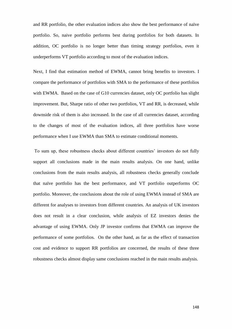
148

and RR portfolio, the other evaluation indices also show the best performance of naïve

portfolio. So, naive portfolio performs best during portfolios for both datasets. In

addition, OC portfolio is no longer better than timing strategy portfolios, even it

underperforms VT portfolio according to most of the evaluation indices.

Next, I find that estimation method of EWMA, cannot bring benefits to investors. I

compare the performance of portfolios with SMA to the performance of these portfolios

with EWMA. Based on the case of G10 currencies dataset, only OC portfolio has slight

improvement. But, Sharpe ratio of other two portfolios, VT and RR, is decreased, while

downside risk of them is also increased. In the case of all currencies dataset, according

to the changes of most of the evaluation indices, all three portfolios have worse

performance when I use EWMA than SMA to estimate conditional moments.

To sum up, these robustness checks about different countries’ investors do not fully

support all conclusions made in the main results analysis. On one hand, unlike

conclusions from the main results analysis, all robustness checks generally conclude

that naïve portfolio has the best performance, and VT portfolio outperforms OC

portfolio. Moreover, the conclusions about the role of using EWMA instead of SMA are

different for analyses to investors from different countries. An analysis of UK investors

does not result in a clear conclusion, while analysis of EZ investors denies the

advantage of using EWMA. Only JP investor confirms that EWMA can improve the

performance of some portfolios. On the other hand, as far as the effect of transaction

cost and evidence to support RR portfolios are concerned, the results of these three

robustness checks almost display same conclusions reached in the main results analysis.

149

5.5 Conclusion

In this chapter, I investigate the performance of optimal constrained (OC) portfolio and

two timing strategy portfolios, volatility timing (VT) portfolio and reward-to-risk (RR)

portfolio for currency market, and compare them to three passive portfolios, which have

good performance in chapter four. The main motivation for this research was to know,

in currencies trading portfolio, whether these portfolios can consistently outperform

naïve portfolio. In addition, in order to reduce estimation error, I also use exponentially

weighted moving average (EWMA) instead of simply moving average (SMA) to

estimate conditional expected moments for the portfolios investigated in this chapter.

Before I started to do the main research, I conducted a Monte Carlo experiment to

understand estimation error, and find improvement on OC portfolio. Due to this error,

the Sharpe ratios of all portfolios except naïve portfolio are lower for out-of-sample

analysis than in sample analysis, while downside risk is raised. But, change for OC

portfolio is not too much. In out-of-sample, I roughly consider that OC portfolio has the

best performance. Only one disadvantage of OC portfolio is that it has high level of

turnover. Hence, the motivation is to use timing strategy to reduce portfolio turnover.

For the US investor using US dollar as the base currency with 5 years estimation

window, there are five main conclusions made. Firstly, again, ‘lesser’ currencies can

give investors an obvious diversification benefit, and then improve the performance.

Secondly, OC and VT portfolio consistently outperforms naïve portfolio in all terms of

evaluation. Thirdly, taking account of return into timing strategy portfolio improved its

performance for all currencies analysis, but did not for G10 currencies analysis.

Therefore, in the case of all currencies dataset, RR portfolio had better performance

than OC and VT portfolios had, and it can also beat minimum variance portfolio. Next,

I found that EWMA is more efficient to estimate conditional expected moments than

150

SMA to reduce estimation error. Finally, transaction cost did not affect the performance

of portfolio significantly regardless of the level of turnover in the case of G10

currencies dataset. But, in the case of all currencies dataset, this effect was very obvious

for the portfolios which have a high turnover. In addition to this main results analysis, I

also conducted a robustness check to investigate whether the conclusions reached are

supported by different lengths of estimation window or other countries’ investors.

Overall, robustness check about different lengths of estimation window confirmed

conclusions reached.

However, robustness checks related to the perspectives of investors from other countries

cannot give consistent conclusions with the main results analysis. There are two main

inconsistent conclusions. The first one was related to comparison of the performance to

naïve portfolio. The results from robustness checks for investors from three

countries/areas, UK, Japan and euro zone, all showed that naïve portfolio has the best

performance in general. But, some portfolios have less downside risk than naïve

portfolio has. The second one was about the role of using EWMA. According to the

results of the analysis for UK investor, it is not clear whether portfolios with EWMA

are better than the ones with SMA. With respect to the analysis for euro zone investors,

the results displayed that using EWMA to replace SMA is useless for improving the

performance of the portfolios. As far as other conclusions are concerned, my robustness

checks had results almost consistent with the main results analysis.

We investigated the performance of OC and timing strategy portfolios for only currency

market. These portfolios are derived from mean-variance model in order to beat naïve

portfolio. However, these strategies also depend on estimation of expected return and

standard deviation of return of currencies. But, once estimating, the error exists. Is there

a possibility of extending to avoid this estimation error? Brandt et al. (2009) give out a

151

strategy named as parametric portfolio policy. This strategy decides weights based on

the characteristics of assets. So, in the next chapter, this strategy will be applied into the

currency market and test if it works or not.

153

Chapter Six

Currency Portfolio Management: Exploiting

Characteristics

6.1 Introduction

All discussion and analysis in preceding chapters are related to the estimation of

expected returns and its covariance matrix. The conclusion shows that the estimation

error impacts performance of portfolio significantly. Although a number of researcher

and literature put lots effort on it to improve the performance, the previous analysis,

DeMiguel et al. (2007) have proved that all extension of Markowitz’s mean-variance

model cannot beat the naïve portfolio. Kirby and Ostdiek (2010) provide simple active

portfolio strategies, called timing strategies, which can outperform naïve portfolio.

Furthermore, chapter five of this thesis shows that these strategies can beat naïve

portfolio in some cases of currencies only portfolio. Unlike extensions of mean-variance

portfolio, the timing strategies rather exploit sample information about the means and

variance of return than focus on optimization method. But, the point is that these

strategies still need to require investors to estimate the first and second moments of

returns of foreign exchange. The main purpose of this chapter is to apply strategies,

which do not require estimating the moments of return, into currency only portfolio. It

is a fact that the return is calculated by exchange rate, and the rate is determined by

some economic factors. I am therefore motivated by following two questions in the first

place to find an alternative approach. Can the factors that determine exchange rate be

154

used to construct a portfolio? Can I build an optimised portfolio by exploiting the

characteristics of currency?

Fortunately, Brandt et al. (2009) provide a guide to answer these questions. They

recommend parametric portfolio policies (PPP) to exploit the characteristics in the

cross-section of equity returns. Specifically, they propose policy weights as a linear

function of characteristics of firm plus benchmark weights. Then, by maximising

average utility of investors, they estimate coefficients of policy. I consider this

alternative strategy as semi-active portfolio, because it seems adjusting benchmark

weights by characteristics. The first term is benchmark weights, which represents

passive element. The second term is adjustment according to the characteristics of asset,

which represents active element. In this chapter, I would like to apply these PPP

strategies into currency only portfolio. But, to implement this, there are two challenges.

One is to select a benchmark portfolio for currency market. Another one is the choice of

the relevant characteristics for this policy.

In response to the first challenge, in the paper of Brandt et al. (2009), they consider

market portfolio weights as benchmark for empirical application. For the FX market,

unlike equity market, there is no market portfolio with value-weighted average. Instead,

I can use GDP or trade weights to construct a market portfolio. However, chapter four

of this thesis has already proved that these two portfolios perform worse than naïve

portfolio. Parametric portfolio policy will be used to adjust a benchmark weight which

has a good performance itself. Therefore, the naïve portfolio could be one of the choices

for the benchmark. In addition, in chapter five, it was concluded that volatility timing

(VT) portfolio has better performance than naïve portfolio in some ways. Moreover, the

features of VT portfolio are similar to the features of naïve portfolio. Although VT

portfolio requires estimating moments, only variance of return needs to be estimated.

155

Therefore, in our empirical application, I consider these two portfolios, naïve portfolio

and VT portfolio, as my benchmark.

With respect to the second challenge, characteristics of currency return are classified,

which are then exploited to construct portfolio, into two parts. The first class is the

financial characteristics, which are derived from three most widely applied currency

trading strategies in practice. One of them is carry trade constructed by borrowing

currency with low interest rate and investing currency with high interest rate (Fama,

1984). This strategy is based on a failure in uncovered interest rate parity, and performs

very well (Burnside et al., 2008). However, it is also well known that the carry trade

faces a substantial crash risk (Brunnermeier et al., 2008; Menkhoff et al., 2012a;

Christiansen et al., 2011). Luckily, since 2008, the other famous currency trading

strategies, the momentum and value, has major development (Menkhoff et al., 2012b;

Burnside et al., 2011; Asness et al., 2013; Jordà and Taylor, 2012). But, these studies

establish one of the strategies or combine them by a simple portfolio (equal weights),

and none of them tries to have optimal portfolio. So, Barroso and Santa-Clara (2011)

explore this undeveloped area by applying parametric portfolio policy. However, in

their approach, the portfolio they build consists of zero sum long-short portfolio and

100% investing in risk free asset, but not benchmark portfolio. This thesis original idea

is to consider characteristics as an opinion of investors to adjust benchmark weights.

Therefore, as discussed before, the naïve portfolio and VT portfolio are used as a

benchmark, and no investment in risk free assets. I consider carry trade (forward

discounts), currency momentum (short term return) and currency value (long term

return) as financial characteristics in my empirical analysis.

The second class is fundamental characteristic. Unlike equity which has characteristics

related to fundamentals of a firm, the fundamental characteristics of currency mostly are

156

related to economic factors of pair countries, and these factors can determine real

exchange rate. The Approach of modelling exchange rate I considered is Behavioural

Equilibrium Exchange Rate (BEER), which extends the relative purchasing power

parity by recognising that the exchange rate is determined by a wide range of

macroeconomic factors. Since Clark and MacDonald (1999) propose BEER model, a

different set of macroeconomic variables are employed in the literature (Komárek et al.,

2005; Lane and Milesi-Ferretti, 2001; MacDonald and Dias, 2007; Cheung et al., 2005).

These models generally offer superior performance in terms of both medium run

valuation and short run dynamics. Hence, the most relevant variables are chosen and,

importantly, they also have to comply with the constraint of data availability. The final

set chosen includes (1) the real interest rate differential, (2) the productivity differential,

(3) the term of trade differential, and (4) the fiscal differential. Adding three

characteristics related to trading strategies, produces seven characteristics. Moreover, I

ran a pre-sample test to determine which characteristics were relevant. This is followed

by a comprehensive out-of-sample analysis with 22 years of weekly returns of G10

currencies to see how PPP portfolio performs.

Moreover, in contrast to researches by Brandt et al. (2009) and Barroso and Santa-Clara

(2011), besides the standard constant relative risk aversion (CRRA) utility function, I

also apply PPP strategy to practitioner-oriented objective function. Concretely, variance

of the portfolio to estimate the coefficients of policy is minimised. As shown in the last

two chapters, minimum variance portfolio has very good performance, even the best

performance sometimes. I also found that it always has the lowest downside risk. In

chapter five, I stated that the investors focus more on risk management; I therefore

estimate the coefficients by minimizing variance of portfolio’s return instead of

maximising utility of investor.

157

The first finding of this chapter is that the fundamental characteristics are efficient out

of the sample for CRRA investors to apply PPP portfolio, but financial characteristics

are not. All terms of evaluation, except CEQ return, do not support PPP portfolio with

financial predictors. Differently, the PPP portfolio with fundamental predictors

performs best in terms of Sharp ratio, CEQ return and Calmar ratio. But, in robustness

check related to Japanese investors, the results do not agree with this outperformance

completely. For Japanese investors, Sharpe ratio of PPP portfolio is not statistically

significantly higher than that of naïve portfolio. Except this disagreement, all other

robustness checks also confirm outperformance of PPP portfolio with fundamental

predictors.

The second finding is that considering all seven characteristics together worsens the

performance of PPP portfolios. Sharpe ratio, Calmar ratio and CEQ return of PPP

portfolio decrease significantly when I combine all predictors into one strategy; and

downside risks increase. This drop leads to the conclusion that PPP portfolio with all

predictors cannot beat naïve portfolio. However, when I consider the perspective of

investors from the UK, PPP portfolio with all predictors has better performance than

naïve portfolio has in terms of evaluation. Even so, the performance of PPP portfolio is

still getting worse after considering all predictors together. For Japanese investors, in

terms of CEQ return and Calmar ratio, PPP portfolio is slightly improved. However,

these inconsistences cannot fully reject these findings. So, it can be said that the

robustness checks generally affirm this finding.

The next finding in this chapter is that the choice of which portfolio weights should be

used as benchmark weights in PPP portfolio is not important to the investor. There is no

significant change in the values of all evaluation indices when I use VT portfolio

weights, instead of naïve weights, as benchmark weights. Therefore, the conclusions

158

remain the same. Furthermore, the results from all robustness checks also consistently

support this finding.

The final finding is that investors may still prefer PPP portfolio to naïve portfolio, if

they firstly think about safety before making an investment. Based on this consideration,

as mentioned before, I estimate coefficients by minimizing a portfolio’s variance rather

than maximising CRRA utility. The results display that PPP portfolio has lower

downside risk than naïve portfolio has. So, given satisfied CEQ returns, the investor

may choose PPP portfolio, although its other evaluation indices are not better than naïve

portfolio’s. This finding is confirmed by robustness check analysis. For UK investor,

Sharpe ratio, CEQ return and Calmar ratio of PPP portfolio are higher than those of

naïve portfolio. This outperformance does not disagree with the findings of this thesis,

but further confirms the finding.

In addition, in this chapter, I document the importance of the currency characteristics

for explaining deviation of PPP portfolio weights from naïve weights. Relative to naïve

weights, the PPP portfolios allocate considerably more wealth to currencies with small

interest rate spread, large real interest rates differential, large productivity differential,

and small term of trade differential.

The rest of the chapter is organised as follows. In section 6.2, a description of

parametric portfolio policy is given. Section 6.3 focuses on the description of currency

characteristics. And, the calculation of predictors is also given in this section. In section

5.4, the results from empirical work are presented. Before out-of-sample analysis, an in-

sample test is done. Finally, section 5.5 gives a conclusion of this chapter.

159

6.2 Portfolio Strategy

In this section, parametric portfolio policy (PPP) will be introduced in detail using

different benchmark portfolio; followed by a description of methods to estimate the

coefficients of the policy.

6.2.1 Basic Approach

Brandt et al. (2009) introduce a simple linear specification for the portfolio weights

function, and his formula showed as follows:

titi

ppp

ti xN

ww ,

'

,,ˆ

1 6.1

where tiw , is the weights of asset i at date t in a benchmark portfolio, is an S*1

vector of coefficient that need to be estimate. tix ,

ˆ is S*1 vector of the characteristics of

asset i , and S is the number of characteristics. This strategy uses a single function of

characteristics to estimate weights for all assets over time, rather than one weight for

each asset at each point in. This is referred to as a portfolio policy.

Again, the strategy captures the idea of active portfolio management. The first term of

the function is benchmark portfolio weights, and the second term, tix ,

' ˆ , is active

element represents opinion of investor to adjust weights from benchmark according to

asset characteristics. These characteristics with zero mean and unit standard deviation

are also standardized. The first reason of standardization is that raw characteristics may

be nonstationary, but standardized characteristics are surely stationary through time.

Secondly, standardization makes sure that sum of deviations from benchmark weights

equal to zero, then the weights of the strategy always sum to one. The term of 1/N can

help investor apply this strategy to an arbitrary and time-varying number of assets.

160

Without this term, when the investment opportunities are not changed fundamentally,

doubling number of asset will result in twice as aggressive allocation. Importantly, the

coefficients, , are constant for all assets and time points. Due to constant coefficients

across assets, the adjustment of weight for each asset is decided by only the

characteristics but not historic performance. This means two assets with similar

characteristics will have similar adjustments even if they have significantly different

historic returns. Coefficients’ being constant through time means that the coefficients

estimated by maximising conditional expected utility of investor at given period are the

same for all periods. So, they also are assumed to maximise the unconditional expected

utility of an investor.

In this chapter, with respect to the benchmark portfolio, I firstly use naïve portfolio,

which equally weight all assets in the portfolio. The equation 6.1 is re-written

corresponding to naïve portfolio as follows:

ti

naiveppp

ti xN

ww ,

'

,ˆ

1 6.2

Secondly, as discussed in section 6.1, I consider VT portfolio instead of naïve portfolio

as benchmark. So, the equation 6.1 is re-written as follows to present that VT portfolio

is concerned.

ti

VT

ti

ppp

ti xN

ww ,

'

,,ˆ

1 6.3

In empirical analysis, I will conduct an out-of-sample analysis to investigate

performance of PPP strategy. Details of the method used about estimating coefficients

are given in the next subsection 6.2.2. In addition, the detail of VT portfolio is given in

the last chapter.

161

6.2.2 Method of Estimating

We have introduced the idea about PPP portfolio. Now, the problem is how to estimate

coefficients of characteristic. Firstly, for the choice of the portfolio weights, investors

would like to maximise the conditional expected utility of investor related to the

portfolio return.

)]([max 1, tpt ruE 6.4

Due to N

i tititp rwr1 1,,1,

the equation 6.4 can be expressed as

)]([max1 !,,

1,

N

i tititwrwuEn

iti

6.5

In the linear policy case 6.1, the optimization problem is

)])ˆ1

(([max1 !,,

'

, N

i tititit rxN

wuE 6.6

Secondly, the important ingredient of the portfolio choice problem is the investor’s

objective function. There are many choices of objective function that can be applied to

this approach, for example, HARA preference, behaviourally motivated utility functions

and practitioner-oriented objective functions. But, in this chapter, I will use standard

CRRA preference to this thesis approach, and the equation is shown below followed

with the expansion form of portfolio return:

1

))ˆ1

(1(

1

)1()(

1

1,1 ,

'

,,1

1,

1,

ti

N

i titititp

tp

rxN

wwrru 6.7

where is a relative risk aversion, and it is set as being equal to 5 as indicated in a

number of literature. The main advantage of CRRA utility is that it penalizes higher-

order moments, unlike mean-variance utility which cares about first and second

162

moments. As far as expected utility is concerned, Brandt et al. (2009) and Barroso and

Santa-Clara (2011) calculate expected utility based on simple average by using the

sample counterparts. However, I will apply exponentially weighted moving average

(EWMA) instead of simple moving average (SMA) to estimate expected utility of

investors. The details of how to apply EWMA has been provided in Chapter 5.

Alternatively, as mentioned before, I also consider a practitioner-oriented objective

function in optimal portfolio policy. Due to good performance of minimum variance

portfolio with the lowest downside risk, I estimate the coefficients of PPP strategy by

minimizing the variance of returns of portfolio for estimation period.

6.2.3 Transaction Cost

In this chapter is concerned with the performance of optimal portfolios after taking into

consideration transaction cost. To do this, in previous chapters, I subtract the effect of

transaction cost from return of portfolio for evaluation period. This means that I take

account of transaction cost only when I evaluate the performance of the portfolio.

However, in this chapter, the coefficients, , are constant in estimation period, but

weights are not. This may lead to unneglectable effect of transaction cost to the return of

portfolio in estimation period. So, I also take account of transaction cost when

estimating coefficients of characteristics of currency. Specifically, the utility function

related to case of taking transaction cost is, now, expressed as follows:

1

))1)()ˆ'1

(1(()~(

1 1

1

,,,,,

1,

N

i

N

i tititititi

tp

crxN

wru 6.8

where tic , the transaction is cost of currency i at time t , and ti , is turnover for

currencies i in optimal portfolio at time t . The methods used to calculate transaction

cost and turnover have been introduced in chapter three. I then maximise expected

163

conditional utility relative to the above equation 6.8 to estimate coefficients of

characteristics. The same process is also applied into estimation about practitioner-

oriented objective function.

6.3 Data

We have already described the calculation of return for currency portfolio in chapter

three. I still use the same approach for calculation, but extend the period to the end of

2014. In this section, I focus on description of characteristics of currency used. The

following economic data is from DataStream.

6.3.1 Financial Characteristics

The first three characteristics considered in this chapter are related to three famous

currency trading strategies. These variables are determined by historical or present

performance of currency. So, I call them financial characteristics. The calculation to

build these three variables in my optimization exercise is:

Carry Trade:

We use the log of forward discount, also referred to as interest rate spread, on currency,

and denote them as )ln(,

1,,

,

ti

tti

tiS

FCT

. I also denote the cross-sectional mean and

standard deviation across all countries available at time t astCT and

tCT respectively. I

standardize the forward discount as:

t

t

CT

CTti

ti

CTct

,

,.

164

Currency Momentum:

We use the log of cumulative currency appreciation in the last four week. So, I calculate

them as )ln(4

,

t

tti

S

SCM . I also apply cross-sectional standardizations according to

t

t

CM

CMti

ti

CMcm

,

,, where

tCM and tCM is mean and standard deviation of

cumulative appreciation cross all countries.

Currency Value:

We use the log of the cumulative real currency change in two years. The formula used

to calculate this variable is )ln(4104,104,

1044,4,

, US

ttiti

US

ttiti

tiCPICPIS

CPICPISCV

. I use two month lag to ensure

the CPI is known. This means that the CPI used in the formula is actually CPI of the

country two months ago, but published currently. To avoid overlap with currency

momentum, I only explore the real currency change between 104t to 4t . Again, I

standardize this variable cross-sectionally, and denote asticv ,.

6.3.2 Fundamental Characteristics

Another class of characteristics in this chapter is related to economic factors of pair

countries. These economic factors chosen are determiners to model currency exchange

rate based on BEER model. I calculate the variables in the empirical analysis as follows.

In addition to calculation, I also give the reason about why these economic factors

should be concerned.

Real Interest Rates Differential:

According to uncover interest parity (UIP), in order to equalise the yields in domestic

and foreign currency, a currency with a positive interest rate is expected to depreciate.

165

Similarly, if interest rate differential increases, the demand for the currency with

relatively higher interest rate will be higher, due to portfolio reallocation. So, I are

suggesting that a positive interest rate differential with respect to foreign currency

should result in contemporaneous appreciation of domestic currency.

We define real interest rates as long term interest rates (usually 10-year government

bond yield) adjusted by a change in CPI from the last year. Specifically, the formula

used to calculate the real interest rates is52,

,

,1

1

tt

ti

tiCPI

bondRIR , where

52, ttCPI present

the rate change from year to year. I obtain the variable by log of quotient of two

countries’ real interest rates, expressed as )ln(,

,

ti

US

tti

RIR

RIRRIRD . And then, I denote the

cross-sectional standardization form of this variable astirird ,.

Relative Price of Non-traded to Traded Goods (Productivity):

If domestic average productivity is higher than foreign economy, the domestic inflation

will be higher, and then typically lead to results in an appreciation of the domestic

currency. This is associated with the Balassa-Samuelson effect. This effect states that

when growth of productivity is relatively higher in domestic tradable sector than in non-

tradable sector, the wages in the tradable sector tend to increase. Under perfect labour

mobility, due to equalization of wages in two sectors, the price of non-tradable goods

will increase. This leads to an increase in overall price level in the domestic economy

with respect to the foreign economy and higher demand for domestic currency relative

to the foreign currency. Finally, appreciation of the real exchange is induced by an

increase in productivity.

166

We define this one as the ratio of CPI to domestic wholesale or producer price index

(PPI), and denote it as )(,

,

,

ti

ti

tiPPI

CPITNT . And then, I calculate variables in log as formula

of )ln(,

,

ti

US

tti

TNT

TNTTNTD . Finally, the cross-sectional standardization form of

tiTNTD ,is

denoted as titntd ,

Term of Trade:

The term of trade is a ratio of export price to import price, which is related to current

accounts and the balance of payments. In a phenomenon of positive shock to term of

trade (a greater rise of export price than risk of import price), rising exports revenues

provide increased demand for the country’s currency, which leads to appreciation.

We denote export and import price index as tiEXPRIN ,and

tiIMPRIN ,, respectively. So,

I define terms of trade asti

ti

tiIMPRIN

EXPRINTOT

,

,

, , and the variable is calculated in logs by

)ln(,

,

ti

US

tti

TOT

TOTTOTD . Again, I need cross-sectional standardization form of this

variable, which denote as titotd , .

Government Consumption:

In the short run, the greater government consumption will induce greater demand of

non-tradable goods, which then increases the overall domestic price level. Consequently,

an appreciation occurs. But, in the long run, growing consumption means more budget

deficit, which could be considered as an unstable economy leading to depreciation.

We consider this variable as log of the ratio of the US government expense, US

tEXPEN ,

to foreign government expense, tiEXPEN , , and the government expense is defined as a

167

ratio of government consumption, tiGOV ,, to nominal GDP,

tiGDP,. The formula is as

follows:

)ln(,

,

ti

US

tti

EXPEN

EXPENGC , where

ti

ti

tiGDP

GOVEXPEN

,

,

, .

After conducting cross-sectional standardization, the variable istigc ,.

6.4 Empirical Analysis

6.4.1 Pre-sample Test

Before conducting out-of-sample analysis, I would like to test the relevance between

variables and weights. To do this, I divide this subsection into two parts. In the first part,

I conduct an in-sample analysis for the period from November 1992 to October 1997. I

apply PPP portfolios with different variable classes to compare their performance.

These classes include seven classes, which only contain single variable respectively,

and one class contains three variables responding to financial characteristics, and one

class contains four variables responding to fundamental characteristics, and the final

class contains all seven variables. So, I have ten PPP portfolios in total. In the second

part, I perform a bootstrap to obtain the p-value of coefficients to make sure that the

coefficients are different from zero. Specifically, I re-sample 1000 random samples of

the same size as the original, drawn with replacement from original sample. Then, I re-

estimate coefficient of variables for each sample. After this, the distribution of

coefficient is constructed, and the p-value is based on student t-statistics with null

hypothesis of zero mean.

6.4.1.1 In sample Analysis

The results of the performance of ten PPP portfolios are shown in

168

Table 6.1. According to the Sharpe ratio, the carry trade delivers the best performance in

all single variable strategies related to financial predictors, with Sharpe ratio of 0.074.

But, carry trade strategy has more crash risk than others, because of higher Kurtosis and

left-skewness, as well as the lowest minimum return. When I consider combining three

financial predictors (including carry trade, currency momentum and currency value) in a

strategy, the improvement of Sharp ratio with an increase of almost 30%, compared to

carry trade strategy, is significant.

As far as fundamental predictors are concerned, the strategy with productivity predictor

(tntd) has the largest Sharpe ratio of 0.177. Moreover, these four strategies have similar

crash risk, except productivity strategy with minimum return of -8.65%. To combine

four fundamental predictors together, I construct a portfolio which improves Sharpe

ratio by 23% compare to productivity strategy. However, it has significant potential risk

to crash, based on extremely large kurtosis. Then, the risk is reduced by adding three

financial predictors. Compared to the strategy with three financial predictors, the

strategy including all variables increases the Sharpe ratio by only 5%. Although, in

terms of Sharpe ratio, financial predictors do not improve this strategy too much, the

crash risk is reduced. Especially, kurtosis indicated 21% crash risk reduced. After

analysing performance of all strategies, I may suggest that there is evidence to support

relevance of variables. The more evidence needed is related to statistical significance of

coefficients of variables.

169

Table 6.1 performance of each strategy for in sample analysis

This table shows the in sample performance of investment strategies for the period of pre-sample (1992-1997). The

aversion coefficient used in CRRA utility is five. The ‘max’ and ‘min’ represent the maximum and minimum of one

week return in the sample. The ‘mean’ is the average return of sample weekly return. The standard deviation, kurtosis

and skewness have abbreviation as ‘Std’, ‘Kurt’ and ‘Skew’ in this table respectively. The ‘SR’ stands for Sharpe

ratio. The first 7 rows show the results of a strategy based on using only one characteristic as variable at a time. The

next 2 rows show the results of a strategy combining different variables. The last row shows the results of a strategy

combining all variable simultaneously. See description of the characteristics variables in the text.

Variable Max Min Mean Std Kurt Skew SR

ct 7.91% -14.57% 0.20% 2.71% 6.499 -0.880 0.074

cm 6.93% -6.34% 0.04% 1.43% 7.542 -0.186 0.031

cv 6.02% -4.83% 0.09% 1.55% 4.259 0.388 0.055

rird 2.62% -6.78% 0.03% 1.20% 6.687 -1.067 0.025

tntd 12.88% -8.65% 0.54% 3.05% 4.156 -0.047 0.177

totd 2.42% -2.44% 0.01% 0.76% 4.110 -0.044 0.017

gc 1.89% -2.59% 0.01% 0.57% 4.233 -0.209 0.018

ct,cm,cv 12.74% -11.20% 0.31% 3.41% 4.156 -0.013 0.091

rird,tntd,totd,gc 37.52% -9.99% 1.06% 4.89% 14.600 1.675 0.218

all 44.81% -14.92% 1.44% 6.29% 11.487 1.518 0.229

170

6.4.1.2 P-value of Bootstrap

Table 6.2 summarises the statistical significance of coefficients of variables for both

single variable and combination strategies. For single variable strategies, coefficients of

all variables are significant at 2% level. Moreover, considering combined strategies for

financial predictors, I conclude that the coefficients are statistically significantly

different from zero, according to p-value of zero. I have known that Burnside et al.

(2011) give explanations of profitability of carry trade and momentum strategies.

Comprehensive evidence on the return premium to value and momentum strategies is

provided by Asness et al. (2013). Barroso and Santa-Clara (2011) also prove that the

carry trade, momentum and value are strong relevant to optimal portfolio. Furthermore,

for a strategy with fundamental predictors, p-values of coefficients of these variables are

zero. The economic factors determine the exchange rate, and therefore have connection

to the return of currency. These factors can be used to construct optimal portfolio.

Moreover, the zero p-values confirm that the variables responding to these economic

factors are relevant to PPP portfolio. After considering all predictors in a strategy, the

p-value of zero displays all coefficients are different from zero in statistically significant

level.

The statistical significance of coefficients of variables confirms the conclusion made

previously. All variables are relevant for the optimization. I will apply all characteristics

(including both financial predictors and fundamentals) in my parametric portfolio policy

for out-of-sample practice.

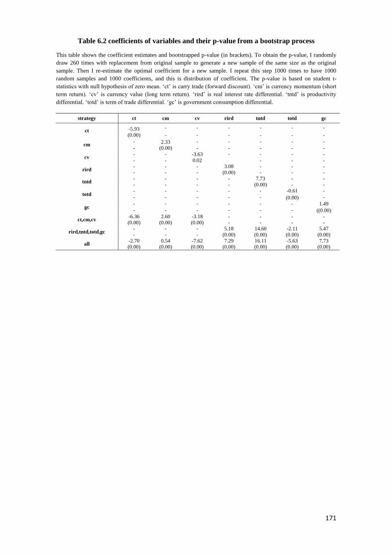
171

Table 6.2 coefficients of variables and their p-value from a bootstrap process

This table shows the coefficient estimates and bootstrapped p-value (in brackets). To obtain the p-value, I randomly

draw 260 times with replacement from original sample to generate a new sample of the same size as the original

sample. Then I re-estimate the optimal coefficient for a new sample. I repeat this step 1000 times to have 1000

random samples and 1000 coefficients, and this is distribution of coefficient. The p-value is based on student t-

statistics with null hypothesis of zero mean. ‘ct’ is carry trade (forward discount). ‘cm’ is currency momentum (short

term return). ‘cv’ is currency value (long term return). ‘rird’ is real interest rate differential. ‘tntd’ is productivity

differential. ‘totd’ is term of trade differential. ‘gc’ is government consumption differential.

strategy ct cm cv rird tntd totd gc

ct -5.93 - - - - - -

(0.00) - - - - - -

cm - 2.33 - - - - -

- (0.00) - - - - -

cv - - -3.63 - - - -

- - 0.02

- - -

rird - - - 3.08 - - -

- - - (0.00) - - -

tntd - - - - 7.73 - -

- - - - (0.00) - -

totd - - - - - -0.61 -

- - - - - (0.00) -

gc - - - - - - 1.49

- - - - - - ((0.00)

ct,cm,cv -6.36 2.60 -3.18 - - - -

(0.00) (0.00) (0.00) - - - -

rird,tntd,totd,gc - - - 5.18 14.60 -2.11 5.47

- - - (0.00) (0.00) (0.00) (0.00)

all -2.70 0.54 -7.62 7.29 16.11 -5.63 7.73 (0.00) (0.00) (0.00) (0.00) (0.00) (0.00) (0.00)

172

6.4.2 Out-of-sample Analysis

In this section, an out-of-sample analysis is performed to check robustness of the

selected strategies. Parameters for parametric portfolio policy are estimated by initial

260 weeks of the sample, which is 5 years from 11.1992-11.1997. The first portfolio is

constructed using these parameters. I then re-estimate parameters every week, using an

expanding estimation window until the end of the sample, 30/12/2014. Expending

estimation window, unlike rolling window I have done in the last two chapters, adds

new week data into window, but not drop the oldest data. The reason I use expending

window rather than rolling window is to minimise the problem of look-ahead bias,

which led by delaying availability of fundamental predictors.

As discussed in the section of pre-sample analysis, all seven variables are incorporated

into optimization strategy. But, taking in isolation, there are two additional optimization

strategies considered as well. One only includes three financial predictors, and the other

one only includes four fundamental predictors. Thus, I can find out which kind of

predictors has contribution for the portfolios. Besides three PPP strategies, I also

perform other optimization strategies for comparing, as well as benchmark naïve

portfolio. Mean-variance strategy is considered as it is a cornerstone of modern

portfolio theory. I also perform minimum-variance portfolio, because it has good

performance in chapter one analysis. Optimal constraints portfolio discussed in chapter

two beats most other portfolios. In addition to simple application, again, there is another

reason that naïve portfolio is treated as the benchmark portfolio. This is from the

conclusion of chapter one, which states that no optimal strategies can beat naïve

portfolio consistently for all terms of evaluation. So, the first part of this section

analyses the PPP strategy, which uses naïve weights as benchmark weights and apply

CRRA utility function to estimate coefficients. Because the motivation of this research

173

is to find out optimal weights derived from naïve weights by active components

(financial and fundamental predictors), in order to test if the active components work, I

compare performance of naïve portfolio to PPP strategies. As already introduced, I also

try to use VT portfolio weights as benchmark weights in PPP strategy. This analysis is

done in the second part of this section. In addition, I minimise variance of portfolio

return to estimate coefficients in the third part of this section.

Due to the fact that economic factors of most developing countries are not available for

the whole period from 1992 to 2014, I only investigate the PPP portfolio for G10

currencies for this period. Then, I conduct robustness check analysis based on the

perspectives of investors from different countries.

6.4.2.1 Basic Case

Table 6.3 shows the results of PPP portfolio with my first scenario, which adjusts

portfolio weights from naïve weights and estimate coefficients by maximising constant

relative risk aversion (CRRA) utility function. In addition to performance of this

portfolio, the table also gives the results of naïve portfolio and other optimal portfolios

to make comparison. As far as PPP portfolio with financial predictors is concerned,

although the Sharpe ratio of it is higher than that of naïve portfolio, the p-value of 0.49

indicates that there is not statistically significantly different between two ratios. CEQ of

1.11% for naïve portfolio means that investors would like to choose naïve portfolio

when certain return is lower than 1.11%. But, CEQ for PPP portfolio with financial

predictors indicates that this certain return is 2.04%. So, when there is a certain return

between 1.11% and 2.04% in the universe of investment, the investor will choose this

PPP portfolio rather than naïve portfolio. Downside risks are higher for PPP portfolio

with financial predictors than naïve portfolio. Moreover, they have the same Calmar

ratios. Therefore, only CEQ supports PPP portfolio with financial predictors, but other

174

evaluations display that naïve portfolio performs better than PPP portfolio with financial

predictors.

To consider only four fundamental predictors, I find that the performance of this PPP

portfolio is better than that of naïve portfolio, as well as PPP portfolio with financial

predictors. According to p-value and return-loss, I can see that Sharpe ratio of PPP

portfolio with fundamental predictors is statistically significantly higher than Sharpe

ratio of naïve portfolio. CEQ of 5.20% indicates that investors more prefer this

portfolio than naïve portfolio and PPP portfolio with financial predictors, when universe

of investment has certain return less than 5.20%. PPP portfolio with fundamental

predictors, indeed, has higher downside risks than naïve portfolio has. But, this portfolio

has Calmar ratio of 0.13 which is higher than 0.06 for naïve portfolio. So, considering

both of return and risk, PPP portfolio with fundamental predictors performs better than

naïve portfolio and PPP portfolio with financial predictors.

For the strategy I combine all predictors, the performance is not improved and even gets

worse. The PPP portfolio’s Sharpe ratio decreases from 0.33 for fundamental predictors,

to 0.20 for financial predictors, and finally to 0.18 for all predictors (For comparison,

Sharpe ratio of naïve portfolio is 0.18). CEQ return of the portfolio, with all predictors,

drops to 1.27% from 5.20% for fundamental predictors. This means that the investor

only chooses PPP portfolio with all predictors when the highest certain return in the

universe of investment is less than 1.27%. Moreover, the downside risks increase, and

Calmar ratio decreases. Compared to naïve portfolio, most of evaluation indices show

that PPP portfolio with all predictors cannot beat naïve portfolio.

175

Table 6.3 Performance of portfolios related to naïve portfolio

This table documents the evaluation of performance of PPP portfolios for US investor’s. This means that the US

dollar is used as the as the base currency. I maximise the CRRA utility to estimate the coefficients, and treated naïve

weights as benchmark weights. The first column, referred as ‘SR’, reports the annualised Sharpe ratio of portfolios. In

the next two columns, ‘vs 1/N’ means that optimal portfolio compare with naïve portfolio. In this category, there are

two comparisons; one is called ‘p-val’, which is the p-value of difference between the Sharpe ratio of each strategy

from that of the 1/N, another one is called ‘re-loss’ refer to return-loss. ‘CEQ’ means annualised certainty-equivalent

return with risk aversion of 5. ‘VaR’ and ‘CVaR’ mean weekly Value at risk and weekly conditional value at risk,

which both are computed at possibility of 95% with historical sample approach. I report two evaluation indices

relevant to drawdown. One is maximum drawdown referred as ‘MDD’, another one is Calmar ratio referred as ‘CR’.

Except VaR, CVaR and maximum drawdown, the results of all other indices are annualised. In addition, I report

turnover only in the part of no transaction cost. I divided this table into two parts. The first part documents the

performance of portfolios without transaction cost. The second part documents the performance after taking account

of transaction cost. For each part, I report seven portfolios. The ‘1/N’ refers to naïve portfolio, which is equally-

weighted. ‘PPP’ represents three PPP portfolios. The first one is PPP portfolio with only three financial predictors,

tagged as ‘Financial’. The second one is PPP portfolio with only four fundamental predictors, tagged as

‘Fundamental’. The third one is PPP portfolio with all predictors, tagged as ‘All’. ‘Other’ represents other optimal

portfolios, including sample based mean-variance portfolio as ‘Mean-var’, minimum-variance portfolio as ‘Min-var’

and optimal constrained portfolio as ’OC’.

SR vs 1/N

CEQ VaR CVaR DD

Turnover

p-value re-loss MDD CR

No transaction cost

1/N 0.18 1.00 0.00% 1.11% 1.81% 2.41% 25.16% 0.06 0.01

PPP

Financial 0.20 0.49 -0.48% 2.04% 4.19% 6.32% 56.75% 0.06 0.53

Fundamental 0.33 0.00 -3.89% 5.20% 5.32% 8.11% 62.68% 0.13 0.75

All 0.18 0.95 -0.07% 1.27% 5.83% 8.64% 68.69% 0.07 1.03

Other

Mean-var -0.01 0.00 46.62% -304.41% 9.74% 47.01% N/A -0.02 382.02

Min-var 0.08 0.00 0.65% 0.31% 1.42% 1.98% 21.76% 0.03 0.02

OC 0.10 0.00 0.51% 0.48% 1.44% 2.03% 22.86% 0.03 0.03

with transaction cost

Naïve 0.17 1.00 0.00% 1.10% 1.81% 2.41% 25.23% 0.06 -

PPP

Financial 0.19 0.70 -0.24% 1.77% 3.85% 5.91% 54.56% 0.06 -

Fundamental 0.29 0.01 -2.72% 4.08% 5.05% 7.76% 60.11% 0.11 -

All 0.14 0.39 0.81% 0.45% 5.42% 8.23% 67.61% 0.05 -

Other

Mean-var -0.25 0.00 1232.88% -42679.14% 10.05% 313.37% N/A -6.88 -

Min-var 0.08 0.00 0.67% 0.29% 1.42% 1.98% 21.81% 0.02 -

OC 0.10 0.00 0.55% 0.42% 1.44% 2.04% 22.95% 0.03 -

176

With respect to other optimal portfolios, they cannot outperform naïve portfolio in terms

of considering both return and risk. Because of negative Sharpe ratio and Calmar ratio

and ridiculous downside risk, sample based mean-variance portfolio performs the worst

among all portfolio strategies. Moreover, its CEQ return indicates that investor will

never choose this portfolio, due to the fact that certain returns will always be higher than

-304.41%. Another two optimal portfolios reported here do not have better performance

than naïve portfolio for some terms of evaluation. So, if I take account of both return

and risk to evaluate the performance, these two optimal portfolios cannot outperform all

PPP portfolios.

The transaction cost impact on the performance of some portfolios in a way. In addition

to high level turnover of sample-based mean-variance portfolio, the PPP portfolios also

have a large turnover. Although transaction cost leads to the fact that Sharpe ratio of

PPP portfolio, with fundamental predictors decreasing from 0.33 to 0.29 and its Calmar

ratio decreases from 0.13 to 0.11, these two ratios are still higher than those of naïve

portfolio. Furthermore, p-value of 0.01 indicates that Sharpe ratios of naïve portfolio

and PPP portfolio with fundamental predictors have statistically significant difference.

However, transaction cost makes PPP portfolio with all predictors have a lower Sharpe

ratio and Calmar ratio than naïve portfolio has. There is no significant effect on three

portfolios, including naïve portfolio, minimum variance portfolio and OC portfolio.

From the table, I can find that downside risks of three PPP portfolios decrease slightly

after taking account of transaction costs. This is an unusual situation when I investigate

the effect of transaction cost in the last two chapters. For other optimal portfolios, I

remove the trading cost for the returns of portfolio when I evaluate them, then the

downside risks should increase. In previous cases and after taking transaction cost, the

portfolios are the same, and the only difference is whether or not I should remove the

trading cost. But, for the PPP portfolios, I also take account of transaction cost when

177

estimating the coefficients to construct portfolios. So, there are two different portfolios

in the cases before and after taking transaction cost. The new portfolio may have lower

downside risks than the original one. After taking transaction cost in evaluation process,

the downside risks of new portfolio can still be lower than those of original portfolio.

6.4.2.2 Benchmark as Volatility Timing Portfolio

In this section, I consider weights of volatility timing (VT) portfolio as benchmark in

PPP strategy, and keep constant relative risk aversion (CRRA) utility function in

estimation process. In addition, I also investigate the performance of VT portfolio for

comparison. The results, shown in Table 6.4, are similar to the last section. Therefore,

the conclusions also are similar to the last section.

Although negative CEQ return means that the investor will never choose VT portfolio,

other evaluation indices support VT portfolio rather than PPP portfolio with financial

predictors. Sharpe ratio of PPP portfolio with financial predictors is 0.19, higher than

0.16 for Sharpe ratio of VT portfolio. But, p-value indicates that there is no statistically

significant difference between two Sharpe ratios. PPP portfolio with financial predictors

has much more downside risk than VT portfolio has, and both portfolios have almost

similar Calmar ratio.

As far as four fundamental predictors are concerned, PPP portfolio has better

performance than VT portfolio has, if the investor cares about trade-off between return

and risk. Comparing to VT portfolio, which Sharpe and Calmar ratios of 0.16 and 0.05

respectively, Sharpe ratio of 0.33 and Calmar ratio of 0.13 for PPP portfolio with

fundamental predictors are very high. P-value also confirms that Sharp ratios for two

portfolios have statistically significant difference. However, if only downside risks are

concerned, they are higher for this PPP portfolio than VT portfolio.

178

Table 6.4 Performance of portfolios related to volatility timing portfolio

This table documents the evaluation of performance of PPP portfolios for US investor’s perspective. This means that

I treated US dollar as the based currency. I maximise the CRRA utility to estimate the coefficients, and treated VT

portfolio weights as benchmark weights. The first column, referred as ‘SR’, reports the annualised Sharpe ratio of

portfolios. In the next two columns, ‘vs VT’ means that optimal portfolio compare with VT portfolio. In this category,

there are two comparisons; one is called ‘p-val’, which is the p-value of difference between the Sharpe ratio of each

strategy from that of the VT portfolio, another one is called ‘re-loss’ refer to return-loss. ‘CEQ’ means annualised

certainty-equivalent return with risk aversion of 5. ‘VaR’ and ‘CVaR’ mean weekly Value at risk and weekly

conditional value at risk, which both are computed at possibility of 95% with historical sample approach. I report two

evaluation indices relevant to drawdown. One is maximum drawdown referred as ‘MDD’, another one is Calmar ratio

referred as ‘CR’. Except VaR, CVaR and maximum drawdown, the results of all other indices are annualised. In

addition, I report turnover only in the part of no transaction cost. I divided this table into two parts. The first part

documents the performance of portfolios without transaction cost. The second part documents the performance after

taking account of transaction cost. For each part, I report four portfolios. The ‘VT’ refers to volatility timing portfolio,

which is introduced in the last chapter. ‘PPP’ represents three PPP portfolios. The first one is PPP portfolio with only

three financial predictors, tagged as ‘Financial’. The second one is PPP portfolio with only four fundamental

predictors, tagged as ‘Fundamental’. The third one is PPP portfolio with all predictors, tagged as ‘All’.

SR vs VT

CEQ VaR CVaR DD

turnover

p-value re-loss MDD CR

No transaction cost

VT 0.16 1.00 0.00% -0.21% 1.61% 2.21% 23.17% 0.05 0.01

PPP

Financial 0.19 0.45 -0.51% 1.73% 3.90% 6.24% 57.13% 0.06 0.52

Fundamental 0.33 0.00 -4.14% 5.00% 5.29% 8.05% 62.73% 0.13 0.74

All 0.17 0.72 -0.37% 1.09% 5.75% 8.57% 68.77% 0.06 1.03


VT 0.16 1.00 0.00% -0.23% 1.61% 2.21% 23.19% 0.05 -

PPP

Financial 0.17 0.60 -0.31% 1.51% 3.68% 5.82% 54.96% 0.05 -

Fundamental 0.29 0.01 -3.13% 4.03% 4.99% 7.76% 60.66% 0.11 -

All 0.13 0.58 0.50% 0.30% 5.41% 8.15% 68.03% 0.05 -

179

If all predictors are considered in one strategy, the performance for this portfolio is

getting worse in all terms of evaluation indices. The Sharpe ratio and Calmar ratio of

PPP portfolio drop from 0.33 and 0.13 for financial predictors to 0.17 and 0.06 for all

predictors, respectively. Change of CEQ indicates that the certain return investor is

expecting decreases from 5% to 1.09%. Moreover, all downside risks of PPP portfolio

increase, when the strategy considers both financial and fundamental predictors together.

With a high level of turnover for all three PPP portfolios, the transaction cost has impact

on their performances, especially Sharpe ratios, but the conclusions remain the same.

Due to low level of turnover, all evaluation indices for VT portfolio are almost

unchanged. For PPP portfolios, these evaluation indices are not unchanged. For

example, turnover of 1.03 makes Sharpe ratio of PPP portfolio with all predictors to

decrease from 0.17 to 0.13, and CEQ drops from 1.09% to 0.3%. However, these

impacts are not enough to change the conclusion made about rankings of performance.

According to the discussion in this and the last sections, I find that Fundamental

characteristics can help investors to improve benchmark portfolio by applying PPP

strategy. Financial characteristics cannot give investor benefits of active portfolio

management in out-of-sample analysis. Moreover, considering both two classes of

characteristics together do not boost the performance of the portfolio, even lead to

worse performance than considering two classes of characteristics separately. In

addition, I realise that the choice of benchmark portfolio is not very important to the

performance of PPP portfolio, as long as they have similar features.

180

6.4.2.3 Minimizing Variance of Return of Portfolio

In this subsection, I estimate coefficients for PPP strategy by minimizing variance of

return of portfolio instead of maximising CRRA utility function. I consider both of two

cases about benchmark portfolio weights. One is to assume that benchmark weights

equal to naïve weights. For another one, VT portfolio is considered as benchmark

portfolio. As illustrated in previous sections, I also report the performance of

benchmark portfolios (naïve and VT portfolios) for comparison. The results are shown

in Table 6.5. It should be noted that I do not report the results of return-loss in this table,

but, instead, I give out two kinds of p-value. The first p-value represents the difference

between relative optimal portfolios and naïve portfolio. And, the second p-value is

about VT portfolio.

With respect to treating naïve portfolio as benchmark, although the PPP portfolios

cannot beat naïve portfolio based on the Sharpe ratio and Calmar ratio, these portfolios

are less risky than naïve portfolio. Sharpe ratios indicate that the performance of PPP

portfolios is not better than that of naïve portfolio, except PPP portfolio with financial

predictors. Especially, zero p-values point out that the difference between their Sharp

ratios is statistically significant. Moreover, Calmar ratios also confirm outperformance

of naïve portfolio when the investor wants to find trade-off between reward and risk.

Nevertheless, because of the fact that the estimation method for coefficients is to

minimise variance of return of portfolios, I assume that investors are more concerned

about downside risk than return. According to VaR, CVaR and maximum drawdown, I

can conclude that three PPP portfolios have lower downside risk than naïve portfolio

has. Furthermore, the lowest CEQ return during these three PPP portfolios is 0.48%.

This means that the investor will choose these portfolios if certain return is lower than

0.48% annually. In practice, this certain return can be considered as risk free rate. For

181

Table 6.5 Performance of portfolios related to minimum variance

This table documents the evaluation of performance of PPP portfolios for US investor’s perspective. This means that I treated US

dollar as the based currency. I minimise variance of return of portfolio to estimate the coefficients. Two cases are reported here. One

is that I treat naïve weights as benchmark weights. Another one is treat VT portfolio as benchmark weights. The first column, referred as ‘SR’, reports the annualised Sharpe ratio of portfolios. In the next two columns, ‘p-value’ means that p-value of

difference between the Sharpe ratio of each strategy from that of relative benchmark portfolio. As I mentioned, there are two

benchmark portfolios. ‘vs 1/N’ ‘reports the p-value against naïve portfolio, and ‘vs VT’ reports the p-value against VT portfolio. I do not report return loss in this table. ‘CEQ’ means annualised certainty-equivalent return with risk aversion of 5. ‘VaR’ and ‘CVaR’

mean weekly Value at risk and weekly conditional value at risk, which both are computed at possibility of 95% with historical

sample approach. I report two evaluation indices relevant to drawdown. One is maximum drawdown referred as ‘MDD’, another one is Calmar ratio referred as ‘CR’. Except VaR, CVaR and maximum drawdown, the results of all other indices are annualised. In

addition, I report turnover only in the part of no transaction cost. I divided this table into two parts. The first part documents the

performance of portfolios without transaction cost. The second part documents the performance after taking account of transaction cost. For each part, I report eight portfolios. The ‘1/N’ refers to naïve portfolio, which is equally-weighted, and ‘VT’ refers to

volatility timing portfolio, which introduced in the last chapter. The rest of portfolios are divided into two categories. The category of ‘Naïve portfolio’ includes PPP portfolios which consider naïve weights as benchmark weights. The category of ‘VT portfolio’

includes PPP portfolios which consider VT portfolio weights as benchmark weights. There are three PPP portfolios included in each

category. The first one is PPP portfolio with only three financial predictors, tagged as ‘Financial’. The second one is PPP portfolio with only four fundamental predictors, tagged as ‘Fundamental’. The third one is PPP portfolio with all predictors, tagged as ‘All’.

SR p-value

CEQ VaR CVaR DD

turnover

vs 1/N vs VT MDD CR

No transaction cost

1/N 0.18 1.00 - 1.11% 1.81% 2.41% 25.16% 0.06 0.01

VT 0.16 - 1.00 -0.21% 1.61% 2.21% 23.17% 0.05 0.01

Naïve

portfolio

Financial 0.18 0.76 - 1.13% 1.77% 2.30% 26.08% 0.06 0.05

Fundamental 0.11 0.00 - 0.53% 1.57% 2.15% 22.78% 0.03 0.05

All 0.10 0.00 - 0.48% 1.52% 2.11% 22.18% 0.03 0.07

VT

portfolio

Financial 0.14 - 0.35 0.76% 1.63% 2.14% 21.93% 0.05 0.04

Fundamental 0.06 - 0.00 0.18% 1.50% 2.06% 24.56% 0.02 0.03

All 0.06 - 0.00 0.20% 1.46% 2.03% 23.43% 0.02 0.05


Naïve 0.17 1.00 - 1.10% 1.81% 2.41% 25.23% 0.06 -

VT 0.16 - 1.00 -0.23% 1.61% 2.21% 23.19% 0.05

Naïve

portfolio

Financial 0.17 0.95 - 1.06% 1.77% 2.31% 26.37% 0.05 -

Fundamental 0.10 0.00 - 0.13% 1.52% 2.07% 23.49% 0.02 -

All 0.09 0.00 - 0.37% 1.52% 2.11% 22.41% 0.03 -

VT

portfolio

Financial 0.13 - 0.16 0.69% 1.63% 2.14% 21.98% 0.04 -

Fundamental 0.04 - 0.00 0.02% 1.46% 2.02% 24.46% 0.01 -

All 0.05 - 0.00 0.12% 1.46% 2.04% 23.90% 0.01 -

182

comparison, I find that annual risk free rates for 1 month and 3 months at the end of

2014 are 0.03% and 0.04% respectively4. So, CEQ returns of portfolios can satisfy the

investor. It is assumed, the investor may prefer PPP portfolio to naïve portfolio because

of low level of downside risk. Therefore, in some ways, this analysis supports PPP

portfolios.

In the case of letting benchmark weights equal to VT portfolio weights, the results are

not changed much, and the conclusions are almost similar to those of naïve portfolio.

P-value indicates that the Sharpe ratios of two PPP portfolios are statistically

significantly different from Sharpe ratio of VT portfolio. Based on the Sharpe ratio and

Calmar ratio, PPP portfolios do not outperform VT portfolio. But, their downside risks

consistently are less than VT portfolio’s. And, PPP portfolio with all predictors has the

lowest downside risk. Moreover, evaluation about CEQ return supports PPP portfolios.

The lowest CEQ return of these PPP portfolios is 0.18%, which is higher than 0.04%

risk free rate for 3 month from US T-bill, but CEQ return of VT portfolio is negative.

Therefore, like conclusions reached in is more analysis of the first case, with enough

CEQ return, the investor, who more concerned with risk than return, may choose PPP

portfolio rather than VT portfolio.

Due to lower level of turnover, the transaction cost effect on the performance of PPP

portfolios is not significant. The largest turnover for PPP portfolios is 0.07, which is

very small, comparing to 1.03 in table 6.3 and table 6.4 which display the performance

of PPP portfolios estimated by maximising CRRA utility function. Sharpe ratio after

taking account of transaction cost only decreases by 0.01 for all PPP portfolios in both

cases. The change of downside risks is also tiny, even some of downside risks is

unchanged. Therefore, I can conclude that transaction cost has an impact on the

performance of PPP portfolios for the cases in this subsection. Then, the conclusions

4 These sources are from official website of U.S. Department of the Treasury.

183

made before taking account of transaction cost are not changed after taking account of

transaction cost.

6.4.3 Robustness Check

As done in previous chapters, I also conduct robustness check to test whether my

conclusions are consistent with different situations. But, unlike the previous chapter, in

this chapter, I only consider perspectives of investors from other countries than US.

Because of the fact that I use extending sample rather than rolling sample to estimate

coefficients, the robustness check for using different lengths of estimation window will

not be very meaningful. If I apply 1 year and 5 years estimation window, for example,

the estimation windows will be mainly different in early period. With extending the

estimation windows, in later years, the difference will be shrinking. So, the 1 year or 5

years only represents initial length of estimation windows, not length for whole period.

Moreover, I use EWMA to weight the historical information. Therefore, the length of

initial estimation windows is not very important to this thesis analysis.

6.4.3.1 UK Investors

In this subsection, in order to perform a robustness check, I investigate the performance

of PPP portfolio related to the perspectives of investor from the United Kingdom. So,

the base currency is Great British pound (GBP) rather than the US dollar. The results

are shown in Table 6.6. I report the performance of naïve and VT portfolio in the first

two rows for comparison with PPP portfolios. I firstly consider naïve portfolio as

benchmark weights, and use CRRA utility function to estimate coefficients. The results

of PPP portfolios related to this case (case one) are given out in Panel A. Secondly, I

keep estimation method as CRRA, but to use VT portfolios weights to represent

benchmark weights. This case is referred as case two, and the results are reported in

184


This table documents the evaluation of performance of PPP portfolios for UK investor’s perspective. This means that I treated British pound as the base currency. The performance of

naïve portfolio and VT portfolio is reported in the first two rows, and referred as ‘1/N’ and ‘VT’ respectively. I firstly consider naïve weights as benchmark weights, and use CRRA

utility function to estimate coefficients. The results of PPP portfolios related to this case are given in Panel A. In Panel B, I keep estimation method as CRRA, but use VT portfolios

weights to represent benchmark weights. In Panel C, I report the results of the case, which estimate coefficients by minimizing variance of return of portfolio and treat naïve weights as

benchmark weights. For each panel, there are three PPP portfolios. The first one is PPP portfolio with only three financial predictors, tagged as ‘Financial’. The second one is PPP

portfolio with only four fundamental predictors, tagged as ‘Fundamental’. The third one is PPP portfolio with all predictors, tagged as ‘All’. In the last panel, Panel D, I report the

performance of two optimal portfolios, including minimum-variance portfolio as ‘Min-var’ and optimal constrained portfolio as ’OC’. The right side of table shows the results before

taking account of transaction cost. The left side of table shows the results after taking account of transaction cost. The first column, referred as ‘SR’, reports the annualised Sharpe ratio

of portfolios. In the next two columns, ‘p-value’ means that p-value of difference between the Sharpe ratio of each strategy from that of relative benchmark portfolio. As I mentioned,

there are two benchmark portfolios. ‘vs Naive’ ‘reports the p-value against naïve portfolio, and ‘vs VT’ reports the p-value against VT portfolio. I do not report return loss in this table.

‘CEQ’ means annualised certainty-equivalent return with risk aversion of 5. ‘VaR’ and ‘CVaR’ mean weekly Value at risk and weekly conditional value at risk, which both are computed

at possibility of 95% with historical sample approach. I report two evaluation indices relevant to drawdown. One is maximum drawdown referred as ‘MDD’, another one is Calmar ratio

referred as ‘CR’. Except VaR, CVaR and maximum drawdown, the results of all other indices are annualised. In addition, I report turnover only in the part of no transaction cost. I

divided this table into two parts. The first part documents the performance of portfolios without transaction cost.

No transaction cost With transaction cost

SR P-value vs

CEQ VaR CVaR DD

turnover SR P-value vs

CEQ VaR CVaR DD

Naive VT MDD CR Naïve VT MDD CR

1/N 0.14 1.00 - 0.69% 1.38% 1.74% 17.85% 0.05 0.01 0.13 1.00 - 0.67% 1.38% 1.74% 18.04% 0.05

VT 0.10 - 1.00 0.43% 1.28% 1.73% 18.91% 0.03 0.01 0.10 - 1.00 0.41% 1.29% 1.73% 19.11% 0.03

Panel A: Naïve portfolio and CRRA utility function

Financial 0.27 0.01 - 3.35% 4.20% 6.33% 42.79% 0.12 0.65 0.22 0.05 - 2.30% 3.83% 5.71% 42.74% 0.09

Fundamental 0.30 0.00 - 4.19% 4.65% 7.28% 46.84% 0.14 0.77 0.23 0.05 - 2.55% 4.48% 6.75% 45.00% 0.10

All 0.25 0.02 - 3.19% 5.83% 8.69% 57.73% 0.11 1.15 0.16 0.58 - 0.95% 5.28% 7.97% 59.43% 0.06

Panel B: VT portfolio and CRRA utility function

Financial 0.26 - 0.00 3.05% 4.20% 6.29% 42.65% 0.11 0.64 0.21 - 0.02 2.02% 3.81% 5.67% 42.60% 0.08

Fundamental 0.28 - 0.00 3.66% 4.55% 7.26% 46.33% 0.13 0.77 0.20 - 0.02 2.09% 4.29% 6.73% 43.76% 0.10

All 0.23 - 0.01 2.66% 5.81% 8.63% 57.64% 0.10 1.15 0.14 - 0.36 0.45% 5.31% 7.92% 59.14% 0.05

Panel C: naïve portfolio and minimum variance of return of portfolio

Financial 0.20 0.02 - 1.10% 1.40% 1.79% 15.11% 0.09 0.04 0.19 0.03 - 1.01% 1.40% 1.79% 15.17% 0.08

Fundamental 0.18 0.05 - 1.00% 1.39% 1.75% 16.10% 0.08 0.02 0.18 0.06 - 0.96% 1.39% 1.75% 16.36% 0.07

All 0.27 0.00 - 1.60% 1.42% 1.81% 14.75% 0.12 0.05 0.25 0.00 - 1.48% 1.43% 1.82% 14.84% 0.11

Panel D: other optimal strategies

Min-var 0.04 0.00 0.00 0.04% 1.31% 1.73% 23.38% 0.01 0.02 0.03 0.00 0.00 0.00% 1.31% 1.73% 23.74% 0.01

OC 0.05 0.00 0.00 0.14% 1.32% 1.74% 22.37% 0.02 0.03 0.04 0.00 0.00 0.07% 1.32% 1.74% 23.04% 0.01

185

Panel B. Thirdly, In panel C, I report the results of case three, which estimates

coefficients by minimizing variance of return of portfolio and treat naïve portfolio as

benchmark weights. As discussed before in the analysis of US investors, the choice of

benchmark weights is not important to the performance of PPP portfolios. Moreover,

from panel A and Panel B of Table 6.6, I also can find that the results for different

benchmark weights are similar. So, here, I do not report the results of the case, which

consider VT portfolio weights as benchmark weights and use minimum variance to

estimate coefficients. Finally, I give the performance of other optimal portfolios,

minimum variance and optimal constrained portfolios, in Panel D.

As far as case one is concerned, the results mainly support the conclusions made before

from US investor analysis. The PPP portfolio with fundamental predictors has the

highest Sharpe ratio, and zero p-value indicates that its Sharpe ratio is statistically

higher than naive portfolio’s. Moreover, the highest Calmar ratio of 0.14 proves the best

performance of this PPP portfolio. CEQ return of PPP portfolio with fundamental

predictors indicates that the investor will prefer this portfolio to a certain return if the

certain return in universe is less than 4.19%. So, like the analysis based on US investor,

if both of return and risk are considered in performance evaluation, the PPP portfolio

with fundamental predictors has the best performance. But, downside risks for PPP

portfolios are higher than those of naïve portfolio very much. Combining both

fundamental and financial predictors in one PPP portfolio cannot improve the

performance. Its Sharpe ratio, Calmar ratio and CEQ return decrease, and downside

risks are increased. In addition to these consistent conclusions, there is one conclusion,

which is not consistent to the analysis based on US investor. Although the performance

of PPP portfolio is getting worse after considering all predictors together, it still has

better performance than naïve portfolio based on the evaluation related to trade-off of

return and risk. Due to high level of turnover for PPP portfolios, the performance of

186

these portfolios has obvious drop. For example, Sharpe ratio of the PPP portfolio with

all predictors decreases from 0.25 to 0.16. And, P-value of 0.58 indicates that its Sharpe

ratio is no longer statistically significantly different from naïve portfolio’s Sharpe ratio.

With respect to case two, the conclusion is also consistent to the analysis based on the

perspective of US investor, which is that the choice of benchmark is not important to

the performance of PPP portfolios. On the other hand, the values of various evaluation

indices are not changed too much. The largest differences of Sharpe ratio and Calmar

ratio between case one and two are 0.02 out of 0.25 and 0.01 out of 0.11 respectively.

Especially, for downside risk, VaR of PPP portfolio with financial predictors stay at

4.20% in both cases, and the biggest change, 0.5% out of 46.84%, happens on

maximum drawdown of PPP portfolio with fundamental predictors. On the other hand,

the main conclusions are the same for case one and case two. Combining both classes of

predictors together cannot improve the performance of PPP portfolio in any term of

evaluation. Moreover, all PPP portfolios also have better performance than benchmark

portfolio (here, referred to VT portfolio) if both risk and return are considered in

evaluation, but downside risk is higher for PPP portfolios than VT portfolios.

Transaction cost leads to a significant decrease in Sharpe ratio, then p-value of 0.36

indicates that the difference of Sharpe ratio between PPP portfolio with all predictors

and VT portfolio is not statistically significant. So, the choice of benchmark weights is

not relevant to efficiency of characteristics of currency in PPP portfolio strategy as long

as the benchmark portfolios have similar features.

In response to case three, I find some inconsistent conclusions to the analysis based on

the perspective of US investor. Firstly, Sharpe ratios of PPP portfolios are all higher

than naïve portfolio, and these differences are statistically significant at confidence level

of 95% according to p-values. The lowest Calmar ratio of PPP portfolios is 0.09, which

187

is higher than that of naïve portfolio. CEQ returns indicate that the investor will choose

PPP portfolios if certain return is between 0.69% and 1.00%. Secondly, although VaR

and CVaR do not support PPP portfolios, downside risk related to maximum drawdown

prefer PPP portfolio to naïve portfolio. Finally, according to Sharpe ratios, Calmar

ratios and CEQ returns, the performance of PPP portfolio is improved by considering all

characteristics of currency together. In addition to these inconsistent conclusions, there

is a consistent conclusion. Due to low turnover, the transaction cost has little effect on

the performance of PPP portfolios. There are tiny decreases/increases after taking

account of transaction cost for all evaluation indices.

Like results from the perspective of US investor, the two optimal portfolios, minimum-

variance portfolio and constrained optimal portfolio, cannot beat two benchmark

portfolios. Their Sharp ratios are lower than naïve and VT portfolios’ very much.

Moreover, the CEQ return and Calmar ratio also prove this underperformance.

Although they have very similar value at risk and conditional value at risk, the

maximum drawdowns of benchmark portfolios are higher than these two optimal

portfolios.

6.4.3.2 Japanese Investors

Here, I focus on the perspectives of Japanese investor to conduct an analysis of PPP

portfolios. So, now, the Japanese yen is a based currency. And, the results are shown in

Table 6.7. The format of this table is similar to the format of Table 6.6. Besides naïve

portfolio and VT portfolio, in four panels, I report the performances related to three

cases of PPP portfolios and two other optimal portfolios.

188


This table documents the evaluation of performance of PPP portfolios for Japanese investor’s perspective. This means that I treated Japanese yen as the base currency. The performance

of naïve portfolio and VT portfolio is reported in the first two rows, and referred as ‘1/N’ and ‘VT’ respectively. I firstly consider naïve weights as benchmark weights, and use CRRA

utility function to estimate coefficients. The results of PPP portfolios related to this case are given in Panel A. In Panel B, I keep estimation method as CRRA, but use VT portfolios

weights to represent benchmark weights. In Panel C, I report the results of the case, which estimate coefficients by minimizing variance of return of portfolio and treat naïve weights as

benchmark weights. For each panel, there are three PPP portfolios. The first one is PPP portfolio with only three financial predictors, tagged as ‘Financial’. The second one is PPP

portfolio with only four fundamental predictors, tagged as ‘Fundamental’. The third one is PPP portfolio with all predictors, tagged as ‘All’. In the last panel, Panel D, I report the

performance of two optimal portfolios, including minimum-variance portfolio as ‘Min-var’ and optimal constrained portfolio as ’OC’. The right side of table shows the results before

taking account of transaction cost. The left side of table shows the results after taking account of transaction cost. The first column, referred as ‘SR’, reports the annualised Sharpe ratio

of portfolios. In the next two columns, ‘p-value’ means that p-value of difference between the Sharpe ratio of each strategy from that of relative benchmark portfolio. As I mentioned,

there are two benchmark portfolios. ‘vs 1/N’ ‘reports the p-value against naïve portfolio, and ‘vs VT’ reports the p-value against VT portfolio. I do not report return loss in this table.

‘CEQ’ means annualised certainty-equivalent return with risk aversion of 5. ‘VaR’ and ‘CVaR’ mean weekly Value at risk and weekly conditional value at risk, which both are computed

at possibility of 95% with historical sample approach. I report two evaluation indices relevant to drawdown. One is maximum drawdown referred as ‘MDD’, another one is Calmar ratio

referred as ‘CR’. Except VaR, CVaR and maximum drawdown, the results of all other indices are annualised. In addition, I report turnover only in the part of no transaction cost. I

divided this table into two parts. The first part documents the performance of portfolios without transaction cost.


SR p-value

CEQ VaR CVaR DD

turnover SR p-value

CEQ VaR CVaR DD

Naïve VT MDD CR Naïve VT MDD CR

Navie 0.39 1.00 - 3.87% 2.66% 3.82% 35.04% 0.13 0.01 0.38 1.00 - 3.84% 2.66% 3.82% 35.07% 0.13

VT 0.37 - 1.00 3.40% 2.42% 3.50% 32.26% 0.12 0.01 0.36 - 1.00 3.38% 2.42% 3.50% 32.32% 0.12


Financial 0.38 0.84 - 5.55% 4.52% 6.90% 60.79% 0.12 0.50 0.31 0.18 - 3.21% 4.16% 6.17% 56.67% 0.09

Fundamental 0.47 0.13 - 9.05% 5.82% 8.99% 66.40% 0.19 0.86 0.38 0.85 - 6.20% 5.24% 8.15% 64.81% 0.14

All 0.47 0.14 - 9.76% 6.68% 10.54% 73.84% 0.20 1.18 0.39 0.98 - 6.87% 6.00% 9.46% 71.52% 0.15


Financial 0.38 - 0.76 5.55% 4.47% 6.80% 60.26% 0.12 0.51 0.30 - 0.29 3.11% 3.96% 6.07% 56.23% 0.09

Fundamental 0.46 - 0.10 8.77% 5.69% 8.94% 65.68% 0.19 0.85 0.37 - 0.96 5.94% 5.19% 8.08% 63.91% 0.14

All 0.46 - 0.09 9.58% 6.77% 10.48% 73.51% 0.20 1.18 0.38 - 0.74 6.70% 5.97% 9.38% 71.10% 0.15


Financial 0.28 0.00 - 2.41% 2.43% 3.48% 39.10% 0.08 0.10 0.25 0.00 - 2.15% 2.44% 3.49% 39.98% 0.07

Fundamental 0.30 0.01 - 2.58% 2.38% 3.22% 38.57% 0.08 0.05 0.29 0.00 - 2.48% 2.38% 3.23% 39.07% 0.08

All 0.23 0.00 - 1.84% 2.34% 3.21% 41.59% 0.06 0.11 0.20 0.00 - 1.59% 2.34% 3.22% 42.37% 0.05


Min-var 0.39 0.96 0.59 3.34% 2.17% 3.07% 33.98% 0.11 0.03 0.38 0.92 0.69 3.26% 2.17% 3.07% 34.25% 0.11

OC 0.36 0.44 0.81 3.16% 2.31% 3.36% 33.61% 0.11 0.05 0.34 0.28 0.59 3.03% 2.31% 3.36% 33.95% 0.11

189

The results for the case one give out some conclusions, which are partly inconsistent

with the analysis based on US investor. According to p-value, I find that all Sharpe

ratios of PPP portfolios cannot be considered to be statistically significantly higher than

that of naïve portfolio anymore. Therefore, after trading off between return and risk, I

cannot conclude that PPP portfolio with fundamental predictors completely beat naïve

portfolio, although CEQ return and Calmar ratio support PPP portfolios. PPP portfolio

with all predictors has slightly higher CEQ return and Calmar ratio than PPP portfolio

with fundamental predictors has. This proves that considering all characteristics

together in the policy somehow improves the performance of PPP portfolio. In addition

to two inconsistent conclusions above, the conclusions related to other aspects are

consistent with the analysis based on US investor. For example, PPP portfolios have

more downside risk than naïve portfolio has.

Comparing results in panel A to Panel B, I find that conclusion about the choice of

benchmark portfolio is similar to that in the analysis based on US investor. The

changes of values of all evaluation indices are not significant. Then, the conclusions

made in case one are also confirmed in case two. Therefore, the choice among different

portfolios for benchmark weights is not important for this thesis conclusion. Because of

a high level of turnover in both cases, transaction cost has obvious effect on the

performance of PPP portfolios. Especially, Sharpe ratios and Calmar ratios drop by

around 20% to 25%, and CEQ returns decrease by almost 50%. But, same as the

analysis based on US investor, these drops cannot change the conclusions made before

taking account of transaction cost.

After I move on to case three, I find that the results from Panel C display similar

conclusions to the analysis based on US investor. PPP portfolios can only be supported

by evaluations related to value at risk and conditional value at risk. Other terms of

190

evaluation show underperformance of PPP portfolios. According to all terms of

evaluation, PPP portfolio with fundamental predictors has the best performance during

all three PPP portfolios. CEQ return of this portfolio is 2.58%, which is lower than that

of naïve portfolio but higher than risk free rate of Japan. For the reference, I use 3

month ‘Gensaki’ repo rate as Japanese risk free rate, and at the end of 2014, this rate is

around 0.1%. Therefore, based on the CEQ return, the PPP portfolios cannot be

rejected by the investor immediately. If the risk of investment is prime consideration to

the investor, he may choose PPP portfolio with fundamental predictors rather than naïve

portfolio because this portfolio has low downside risk. Moreover, low level of turnover

leads to very small effect of transaction cost on the performance of PPP portfolios, thus

the conclusions remain unchanged..

6.4.3.3 Euro Zone Investors

In this subsection, I conduct a robustness check based on the perspectives of euro zone

investors. So, euro will be treated as the base currency. I use same format as used in the

previous two subsections to report the results of this robustness check in Table 6.8.

Overall, the conclusions from these results are mostly consistent with the conclusions

from analysis based on US investor. In the following paragraphs, I give these consistent

conclusions in detail for the three cases.

For case one, the PPP portfolio with fundamental predictors displays an outstanding

performance in terms of evaluation related to both risk and return. Firstly, p-value of

0.02 indicates that Sharpe ratio of PPP portfolio with fundamental predictors is

statistically significantly higher than Sharpe ratio of naïve portfolio. Although this PPP

portfolio has more downside risk than naïve portfolio has, the Calmar ratio of this PPP

portfolio is over twice as that of naïve portfolio. Secondly, PPP portfolio with financial

predictors has a Sharpe ratio, which is not statistically significantly different from

191

Table 6.8 Robustness results for perspective of Euro investors

This table documents the evaluation of performance of PPP portfolios for euro zone investor’s perspective. This means that I treated euro as the based currency. The performance of naïve

portfolio and VT portfolio is reported in the first two rows, and referred as ‘1/N’ and ‘VT’ respectively. I firstly consider naïve weights as benchmark weights, and use CRRA utility

function to estimate coefficients. The results of PPP portfolios related to this case are given in Panel A. In Panel B, I keep estimation method as CRRA, but use VT portfolios weights to

represent benchmark weights. In Panel C, I report the results of the case, which estimate coefficients by minimizing variance of return of portfolio and treat naïve weights as benchmark

weights. For each panel, there are three PPP portfolios. The first one is PPP portfolio with only three financial predictors, tagged as ‘Financial’. The second one is PPP portfolio with

only four fundamental predictors, tagged as ‘Fundamental’. The third one is PPP portfolio with all predictors, tagged as ‘All’. In the last panel, Panel D, I report the performance of two

optimal portfolios, including minimum-variance portfolio as ‘Min-var’ and optimal constrained portfolio as ’OC’. The right side of table shows the results before taking account of

transaction cost. The left side of table shows the results after taking account of transaction cost. The first column, referred as ‘SR’, reports the annualised Sharpe ratio of portfolios. In the

next two columns, ‘p-value’ means that p-value of difference between the Sharpe ratio of each strategy from that of relative benchmark portfolio. As I mentioned, there are two

benchmark portfolios. ‘vs 1/N’ ‘reports the p-value against naïve portfolio, and ‘vs VT’ reports the p-value against VT portfolio. I do not report return loss in this table. ‘CEQ’ means

annualised certainty-equivalent return with risk aversion of 5. ‘VaR’ and ‘CVaR’ mean weekly Value at risk and weekly conditional value at risk, which both are computed at possibility

of 95% with historical sample approach. I report two evaluation indices relevant to drawdown. One is maximum drawdown referred as ‘MDD’, another one is Calmar ratio referred as

‘CR’. Except VaR, CVaR and maximum drawdown, the results of all other indices are annualised. In addition, I report turnover only in the part of no transaction cost. I divided this table

into two parts. The first part documents the performance of portfolios without transaction cost.


SR p-value

CEQ VaR CVaR DD

turnover SR p-value

CEQ VaR CVaR DD

Naïve VT MDD CR Naïve VT MDD CR

Navie 0.21 1.00 - 1.03% 1.22% 1.65% 20.61% 0.06 0.01 0.21 1.00 - 1.01% 1.22% 1.65% 20.71% 0.06

VT 0.15 - 1.00 0.51% 0.76% 1.18% 18.96% 0.03 0.01 0.15 - 1.00 0.49% 0.76% 1.18% 19.04% 0.03


Financial 0.30 0.11 - 3.71% 3.89% 6.16% 55.60% 0.09 0.59 0.27 0.20 - 3.09% 3.51% 5.72% 53.28% 0.08

Fundamental 0.37 0.02 - 5.80% 4.74% 7.73% 58.70% 0.14 0.72 0.30 0.11 - 4.13% 4.41% 7.31% 59.27% 0.11

All 0.27 0.28 - 3.64% 5.66% 8.94% 67.39% 0.10 1.08 0.20 0.92 - 1.94% 5.29% 8.27% 66.00% 0.07


Financial 0.30 - 0.03 3.68% 3.81% 6.12% 55.70% 0.09 0.58 0.28 - 0.04 3.09% 3.52% 5.64% 53.41% 0.08

Fundamental 0.34 - 0.01 5.15% 4.90% 7.72% 57.50% 0.13 0.73 0.27 - 0.05 3.49% 4.51% 7.23% 56.59% 0.10

All 0.25 - 0.13 3.01% 5.46% 8.82% 66.79% 0.09 1.07 0.17 - 0.61 1.34% 5.12% 8.11% 65.35% 0.06


Financial 0.13 0.00 - 0.58% 1.23% 1.66% 23.75% 0.03 0.03 0.12 0.00 - 0.50% 1.23% 1.67% 24.11% 0.03

Fundamental 0.35 0.01 - 1.62% 1.01% 1.41% 16.18% 0.11 0.03 0.34 0.00 - 1.64% 1.06% 1.44% 16.19% 0.11

All 0.37 0.00 - 1.75% 0.98% 1.40% 15.98% 0.12 0.06 0.34 0.01 - 1.61% 0.98% 1.41% 16.73% 0.10


Min-var 0.20 0.85 0.16 0.71% 0.71% 1.21% 19.34% 0.04 0.01 0.20 0.79 0.15 0.69% 0.71% 1.21% 19.42% 0.04

OC 0.19 0.63 0.29 0.73% 0.89% 1.34% 20.83% 0.04 0.03 0.17 0.37 0.42 0.66% 0.89% 1.34% 21.07% 0.04

192

Sharpe ratio of naïve portfolio. Thirdly, according to decrease of Sharp ratio and

increase of downside risk, I find that considering all predictors together does not

improve but worsens the performance of PPP portfolio. So, like analysis based on US

investor, only PPP portfolio with fundamental predictors has better performance than

naïve portfolio has, if both of return and risk are considered in evaluation. From results

in panel D, I can find that minimum variance portfolio and optimal constrained portfolio

perform better than naïve portfolio. But, Sharpe ratios and Calmar ratios still confirm

the best performance of PPP portfolio with fundamental predictors. In addition, high

turnover leads to big drop of Sharpe ratio of PPP portfolio with fundamental. The

Sharpe ratio decreases from 0.37 to 0.30, and the value of p-value increases to 0.11. So,

this means that, after taking account of transaction cost, Sharpe ratio of PPP portfolio

with fundamental predictors is no longer higher than that of naïve portfolio in

statistically significant difference.

Comparing results of case two to case one, I conclude that the choice of benchmarks is

not important to investors who want to apply PPP strategy. The changes of all terms of

evaluation can be ignored. From case one to case two, for example, Sharpe ratio of PPP

portfolio with fundamental predictor decreases by 0.03 from 0.37 to 0.34, and this

decrease is largest during all Sharpe ratios. The biggest change for the value of

downside risk is VaR of PPP portfolio with all predictors, which lowers to 5.46% from

5.66%. In addition to these tiny changes of performance evaluation, the changes of

turnover are also small. For three PPP portfolios, the turnovers decrease by only 0.01

relative to the smallest value of 0.58. Therefore, after taking account transaction cost,

the results of case one are also similar to the results of case two. Because of very small

change, the main conclusions in case two are same as the conclusion in case one.

193

The results in panel C about case three display that, except PPP portfolio with financial

predictors, other two PPP portfolios have outperformance over naïve portfolio in all

terms of evaluation, and other two optimal portfolios in most terms of evaluation. As far

as PPP portfolio with financial predictors is concerned, p-value indicates that its Sharpe

ratio is statistically significant lower than Sharpe ratio of naïve portfolio. Other

evaluation indices also confirm that naïve portfolio has better performance than it has.

However, other two PPP portfolios have larger Sharpe ratios than naïve portfolio has.

And, p-value proves that these differences are statistically significantly different.

Moreover, their downside risk is consistently less than naïve portfolio’s. CEQ return

and Calmar ratio also confirm outperformance of PPP portfolio with fundamental

predictors and PPP portfolio with all predictors. Comparing to the performance of other

optimal portfolios, I find that, except VaR and CVaR, all terms of evaluation show

better performance of these two PPP portfolios than minimum-variance portfolio and

OC portfolios. Although above conclusions are not consistent with the conclusions from

analysis based on US investor, overall, the results of this analysis, here, also support

PPP portfolios. In addition, transaction cost does not have significant impact on the

performance of the portfolios.

6.4.4 Investigation of Coefficients for Out-of-sample Analysis

After discussing the performance of PPP portfolios, I investigate the coefficients

corresponding to various predictors for the out-of-sample analysis in this section. Table

6.9 presents the average of estimated coefficients of PPP portfolios related to the basic

case, which treats naïve portfolio weights as benchmark weights and use constant

relative risk aversion (CRRA) utility function to estimate coefficients. Besides US

investors, I also report these estimated coefficients from robustness check analysis.

194

According to this investigation, I can find how the predictors affect weights of PPP

portfolios.

From the signs of coefficients, I can find that the effects of the predictors on weights are

consistent for all portfolios and all perspectives of investors from different countries.

The coefficients corresponding to carry trade (forward discount or interest rate spread),

currency value (long term return) and differential term of trade are negative for all PPP

portfolios related to all four countries/area investors, and the coefficients corresponding

to other predictors are positive. This means that the deviations of the optimal weights

from the benchmark weights decrease with forward discount, long term return and

differential term of trade and increase with short term return (currency momentum),

differential real interest rate, differential productivity and differential government

consumption. Therefore, the investors overweight the currencies have small interest rate

spread, short term winning, long term losing, large real interest rates differential, strong

productivity differential, small term of trade differential, and great fiscal differential and

underweight the currencies have large interest rate spread, short term losing, long term

winning, small real interest rates differential, small productivity differential, large term

of trade differential, and low fiscal differential. This conclusion is also consistent with

the results of Table 6.2 in pre-sample analysis. I can compare the coefficients of each

other, because of the fact that predictors are standardized cross-sectionally.

Quantitatively, a high differential of productivity leads to the largest overweighting of a

currency. However, the short term return, long term return and government

consumption have relatively small effect on the weights, since their coefficients are not

significant.

195

Table 6.9 The average of coefficients for all out-of-sample analyses

This table shows the average coefficients corresponding to their predictors for out-of-sample in main analysis and

robustness analysis. The results related to my main analysis are reported in the first part, referred as ‘US investor’. In

the second part, referred as ‘UK investor’, the results are related to the robustness check based on the perspective of

UK investor. The third part, referred as ‘Japanese investor ’, reports results related to the robustness check based on

the perspective of Japanese investor. The final part, referred as ‘euro zone investor’, reports results related to the

robustness check based on the perspective of euro zone investor. For each part, there are three PPP portfolios. The

first one is PPP portfolio with only three financial predictors, tagged as ‘Financial’. The second one is PPP portfolio

with only four fundamental predictors, tagged as ‘Fundamental’. The third one is PPP portfolio with all predictors,

tagged as ‘All’. For each column, ‘ct’ is predictor of carry trade (forward discount). ‘cm’ is currency momentum

(short term return). ‘cv’ is currency value (long term return). ‘rird’ is real interest rate differential. ‘tntd’ is

productivity differential. ‘totd’ is term of trade differential. ‘gc’ is government consumption differential.

strategy ct cm cv rird tntd totd gc

US investor

Financial -3.41 0.94 -0.45 - - - -

Fundamental - - - 4.81 8.39 -2.68 1.32

All -1.59 0.55 -0.13 5.50 7.94 -2.33 1.07

UK investor

Financial -3.76 1.47 -0.40 - - - -

Fundamental - - - 4.98 7.32 -3.47 1.08

All -4.11 1.00 -0.08 6.03 5.27 -2.23 1.64

Japanese investor

Financial -4.03 0.16 -0.57 - - - -

Fundamental - - - 4.78 9.43 -4.83 1.21

All -4.61 0.55 -1.01 5.88 7.37 -4.79 1.33

euro zone investor

Financial -3.76 1.18 -0.32 - - - -

Fundamental - - - 4.52 7.59 -3.58 2.25

All -3.89 0.75 -0.10 5.74 5.72 -2.60 2.60

196

6.5 Conclusion

In this chapter, the performance of PPP portfolios with different classes of predictors

and different objective functions for currency market is investigated, and compared to

the relevant benchmark portfolios and other optimal portfolios, which have good

performance as outlined in the last chapter. The main motivation of this research was to

find a methodology to construct currency only portfolios based on the characteristics of

currencies, and how these portfolios perform in out-of-sample. I tried to apply

parametric portfolio policy (PPP), proposed by Brandt, Santa-Clara and Valkanov

(2009), to currency only portfolio optimization. I used naïve weights and volatility

timing (VT) portfolio weights as benchmark weights. Two objective functions were

chosen for estimating coefficients. One is constant relative risk aversion (CRRA) utility

function. Another one is practitioner-oriented to minimise variance of return of portfolio.

Moreover, I exploited seven characteristics of currency, divided into two classes. The

first class is financial characteristics, including forward discount, short long return, and

long term return. The second class is fundamental characteristics based on behavioural

equilibrium exchange rate model, including real interest rates, productivity, term of

trade, and government consumption. Before I began the out-of-sample analysis, I

conducted an in-sample analysis to test the relevance of these characteristics to

optimization, and the results are satisfactory. Therefore, in out-of-sample analysis, I had

three portfolios for each case. One included three financial characteristics, and the other

one included four fundamental characteristics, and finally one included all seven

characteristics.

There are four main conclusions made in out-of-sample analysis. Firstly, fundamental

characteristics can give CRRA investor benefits of active portfolio management, but

financial characteristics cannot. Secondly, considering all seven characteristics together

197

worsens the performance of PPP portfolios. Thirdly, the choice of benchmark weights

does not have significant effect on the performance of PPP portfolios. Finally, if the

investors are not CRRA investor, but they would like to minimise portfolio’s variance,

PPP portfolios are still their choice in a way. In addition, the transaction cost does not

change the conclusions reached, although the Sharpe ratios of PPP portfolio, indeed,

decrease distinctly after taking account of transaction cost.

The most conclusions in robustness check analysis are consistent with the above

conclusions, but some of them are inconsistent. For UK investors, the inconsistences are

related to the case, which estimates coefficients by minimizing variance of return of

portfolio. But, these inconsistences cannot reject my conclusion about support of PPP

portfolio. For Japanese investor, CRRA investor will not choose PPP portfolio with

fundamental predictors based on the term of Sharpe ratio. But, it still has the advantage

in terms of Calmar ratio and CEQ return. For euro zone investor, all conclusions are

consistent. Therefore, although inconsistent conclusions exist in robustness check

analysis, the four main conclusions, are robust from the perspectives of investors from

different countries.

The value of coefficients displays a conclusion about how characteristics of currency

make that PPP portfolio weights deviate from benchmark weights, and this conclusion

is consistent with all cases of out-of-sample analysis. Relative to naïve weights, the PPP

portfolios allocate considerably more wealth to currencies with small interest rate

spread, large real interest rates differential, strong productivity, and small positive shock

to term of trade.

199

Chapter Seven

Conclusion and Future Research

7.1 Conclusion

This thesis mainly focuses on the currency only portfolio, and considers investment in

currency market as a speculating opportunity rather than hedge tool. So, I therefore

investigate the out-of-sample performance of various optimal currency only portfolios

(passive and active), and compare them to the performance of naïve portfolio. The

results show that some of passive portfolio strategies cannot beat naïve portfolio, but the

active strategies I investigate in this thesis have better performance than naïve portfolio

has.

We analyse 12 passive portfolio strategies, three non-optimal (benchmark) portfolios

and 9 optimal portfolios, for currency only portfolio in chapter four. Three benchmark

portfolios include naïve portfolio, GDP portfolio and Trade portfolio, and 9 optimal

portfolios include sample-based mean-variance portfolio, its extensions, minimum

variance portfolio and equally-weighted risk contribution portfolio. Like equity

portfolio, the sample-based mean-variance portfolio should have the best Sharpe ratio

in-sample. And, its other evaluation indices also kept at a good level. In the out-of-

sample analysis, however, the results show that the sample-based mean-variance

portfolio works very badly with low Sharpe ratio and horrible downside risk, because of

estimation error. Moreover, the minimum variance portfolios, with and without short-

sale constraint, has the best performance and exposure to the lowest downside risk. The

naïve portfolio and equally-weighted risk contribution portfolio also perform reasonable

well. In addition, adding ‘lesser’ currencies can help investors gain the benefit from

200

diversification. Although transaction cost leads to decreases in the performance of

portfolio with high level of turnover, the rankings do not change after taking account of

transaction cost.

In chapter 5, I analyse optimal constrained portfolio strategy, which derive from mean-

variance optimization with purpose to outperform naïve portfolio, and a class of active

portfolio strategies (called as timing strategy), which include volatility timing strategy

and reward-to-risk timing strategy, for currency only portfolio. In the literature, for the

equity portfolio, the optimal constrained portfolio generally performs better than naïve

portfolio in the absence of transaction costs. And, both types of timing strategies can

outperform naïve portfolio for a range of equity data after high transaction cost is

incorporated. For this thesis analysis about currency only portfolio, optimal constrained

and volatility timing portfolio consistently outperform naïve portfolio in all terms of

evaluation used. However, taking account of return into timing strategy portfolio

improves its performance only for all currencies dataset, but does not for G10 currencies

dataset. Similarly, the transaction cost has obvious effect on the performance of optimal

constrained portfolio for all currencies dataset. But, in the case of G10 currencies

dataset, transaction cost does not affect the performance of optimal constrained portfolio.

In addition, it can be concluded that exponentially weighted moving average is more

efficient to estimate conditional expected moments than simple moving average to

reduce estimation error. Same as chapter 4, ‘lesser’ currencies can give investor an

obvious diversification benefit, and then improve the performance.

In chapter 6, I analyse an alternative active portfolio strategy, which is called PPP

portfolios whose weights deviate from benchmark weights based on the characteristics

of currencies. I used naïve weights and volatility timing portfolio weights as benchmark

weights. And, two objective functions are chosen to estimate coefficients. One is

201

constant relative aversion utility function. Another one is practitioner-oriented to

minimise portfolio’s variance. Besides all seven characteristics together, I also isolate

them with two classes, financial and fundamental characteristics. The results of the out-

of-sample analysis about currency only portfolio show that fundamental characteristics

can give CRRA investor benefits of active portfolio management, but financial

characteristics cannot. The performance of PPP portfolio is worsened if I consider all

seven characteristics together. Moreover, the choice of benchmark weights is not

important to the investor. If the investors are safety-first rather than CRRA investor, the

PPP portfolio still is their choice in a way. Although a high level of turnover of PPP

portfolios, the transaction cost does not change the conclusion. In addition, I find that

the PPP portfolios allocate considerably more wealth to currencies with small interest

rate spread, large real interest rates differential, strong productivity differential, and

small term of trade differential.

The overall results indicate that currencies can be thought of as an asset in their own

right to construct optimal portfolios, which have better performance than naïve portfolio

has, if the suitable strategies are used. Although sample-based mean-variance portfolio

and its extensions do not have very good performance, minimum variance portfolio can

beat naïve portfolio and other market portfolios of currency. A more advanced version

of mean-variance portfolio, optimal constrained portfolio, also has better performance

than naïve portfolio has. For active portfolio management, the two active strategies,

timing strategy and PPP strategy give investors more benefit than naïve strategy Even,

these two active portfolios outperform optimal passive portfolios, e.g. minimum-

variance portfolio and optimal constrained portfolios. Moreover, in the analysis of PPP

portfolios, I find the relationship between characteristics of currency and deviation of

PPP portfolio weights from naïve weights. However, besides what has been researched

202

in this thesis, there are lots things that can be investigated in the future. The next section

will give directions to possible future researches.

7.2 Limitation

There is a potential limitation of the empirical analysis in this thesis. I do not consider

much more about the impact of outliers when I conduct parametric statistics. The

outliers are defined differently, such as Dixon (1950) defines outliers as values that are

‘dubious in the eyes of the researcher’ and Hawkins (1980) describes an outlier as an

observation that ‘deviates so much from other observation as to arouse suspicions that it

was generated by a different mechanism’. But, then, an outlier is generally considered

as a data point which is far away from norm for a variable or population (e.g., Jarrell,

1992; Rasmussen, 1988; Stevens, 1984). Wainer (1976) also introduce fringelier, a

special case of outlier.

Most parametric statistics, like means, standard deviation, and correlations, and every

statistic based on these, are highly sensitive to outliers. Zimmerman (1998) state that the

presence of outlier will lead to inflated error rates and substantial distortions of

parameter and statistics estimates. Schwager and Margolin (1982) also argue that

outliers can seriously bias or influence estimates. However, in this paper, I only checked

the presence of outlier by visual inspection and my experience, but not a certain rule.

Simple rules, such as data point three or more standard deviations from means, are

simple and effective, although some researchers (e.g., Selst and Jolicoeur, 1994)

propose several complex rules. So, the limitation of my empirical analysis is that I do

not use a certain rule to identify the outliers of my data. This may lead to a different

conclusion.

203

There is much debate about how to deal with outliers. When the outliers are

illegitimately, they should be removed from data in common sense (Bamnett and Lewis,

1994). However, when the outliers are legitimately or the cause is unclear, the issue will

be complicated. Judd and McClelland (1989) very support for removal of outliers, and

make several strong points. Osborne and Overbay (2004) empirically demonstrate the

benefits of outlier removal. But, Orr et al. (1991) ague that data are more like to be

representative of the population as a whole if outliers are not removed. In addition to

removal, alternative methods to accommodating outliers include transformation

(Hamilton, 1992; Osborne, 2002) and ‘robust’ procedures (Bamnett and Lewis, 1994).

So, researcher should make decisions on dealing with legitimately by using their

training, intuition, reasoned argument and thoughtful consideration.

7.3 Future Research

Although I have undertaken an analysis in my thesis to investigate the performance of

currency only portfolios related to various optimal strategies, there are still issues that

can be researched in the future.

Firstly, due to the fact that the new strategies will be proposed continuously, it is

interesting to investigate their performance for currency only portfolios. I investigated 9

optimal portfolios (adding 3 market portfolios to have total 12 portfolios) in chapter

four, but there are other optimal portfolio strategies based on improving the estimation

of moments of asset returns can be applied into currency market. Garlappi et al. (2007)

propose a strategy for an investor who has multiple priors and ambiguity aversion. In

their approach, the multiple priors are characterized by a confidence interval around the

estimated expected returns, and a minimization over the priors is used to show

investor’s aversion to ambiguity (uncertainty of estimation). Based on Garlappi’s (2007)

approach, Fonseca et al. (2011) investigate robust optimization for currency only

204

portfolio. They adjust the original idea to comply a feature of currency, which is a

triangular relationship exists among foreign exchange rate. Above is an example about

applying other optimal portfolio strategy into currency only portfolio. Another example

is Bayesian ‘Data-and-Model’ approach proposed by Pástor (2000) and Pástor and

Stambaugh (2000). This approach is Bayesian portfolio based on belief in a particular

asset-pricing model. So, for the future research, I could employ this portfolio strategy to

currency market. Because currency differs from equity, asset-pricing model for the

currency will also differ from asset-pricing model for equity. For example, I may use

currency trading strategies, such as carry trade and momentum trade, to build factors

model as asset-pricing model. However, the research of asset-pricing model on currency

is limited. For the future research in this direction, I could also pay close attention to

more advanced strategies, which may be proposed in the future.

Secondly, rather than weekly data, I could use monthly data to conduct my analysis in

the future. In this thesis, I chose to use weekly frequency for data collection. The

reason is that I would like to obtain enough observations given that the period is limited.

But, for the risk free rate, due to availability of one week and one month T-bills, I only

can use 3 month T-bills with weekly frequency to calculate excess return. Moreover, in

the literature about portfolio strategy, they mostly prefer monthly data. For example, it

includes the papers I mentioned in the thesis, such as DeMiguel et al. (2007), Kan and

Zhou (2007) and Brandt, Brandt et al. (2009). With time permitting in the future, I could

try to collect data on a monthly basis, and use one month T-bills with monthly

frequency to calculate excess return.

Thirdly, more sophisticated estimation techniques could be used to estimate moments of

excess return for timing strategies. In chapter five, I used two estimation techniques,

simple moving average and exponentially weighted moving average, to estimate

205

variance and mean of currency excess return. From the results, I found that

exponentially weighted moving average is more efficient than simple moving average

for my timing strategy. So, it would be interesting to know whether more sophisticated

estimation techniques can bring investors more benefits. For example, I might use

GARCH (1, 1) process to model the daily excess return on each currency. Then, the

forecasts of daily excess return variances are calculated to construct forecasts of

monthly excess return variances. But, this technique requires me to switch to daily data.

So, I could leave this idea to future research.

I also could investigate the reason of inconsistent conclusions in robustness check

analysis. In the conclusion sections of my three main chapters, I have stated some

inconsistences from robustness check related to perspectives of investors from different

countries. Although most of the inconsistences cannot totally reject my main

conclusions, they, at a certain extent, affect investor’s decision for portfolio strategy.

Therefore, it would be interesting to investigate how these inconsistences happen.

Finally, for the PPP portfolio, I could investigate the reason of the fact that financial

characteristics cannot give investor benefit of active portfolio management, and whether

the benefit from fundamental characteristics is likely to continue going forward. In

chapter six, I stated that PPP portfolio with financial predictors cannot beat naïve

portfolio, and they have similar Sharpe ratio and Calmar ratio. One of the explanations

of this phenomenon may be that the currency market is efficient enough to eliminate the

benefit from trading at these financial characteristics. Similarly, the explanation of

outperformance of PPP portfolio with fundamental predictors may that the inefficient

market cannot eliminate the benefit from trading at four fundamental characteristics. To

investigate this, I may test whether the profitability of the PPP portfolios compensate

for the risk they bear. However, according to the adaptive markets hypothesis, Lo

206

(2004) argues that abnormal profitability can persist for some time because the market

needs time to fully arbitrage, but not indefinitely. This also opens a question to

investigate whether the performance of this PPP portfolio is decreasing, and the

outperformance will be eliminated in future. This presents a good opportunity for future

research.

207

References

AIT-SAHALIA, Y. & BRANDT, M. W. 2001. Variable selection for portfolio choice.

National Bureau of Economic Research.

AKGIRAY, V. 1989. Conditional heteroscedasticity in time series of stock returns:

Evidence and forecasts. Journal of business, 55-80.

ALBANESE, C. 1997. Credit exposure, diversification risk and coherent VaR. Preprint,

Department of Mathematics, University of Toronto.

ASNESS, C. S., MOSKOWITZ, T. J. & PEDERSEN, L. H. 2013. Value and

momentum everywhere. The Journal of Finance, 68, 929-985.

BALABAN, E., BAYAR, A. & FAFF, R. W. 2006. Forecasting stock market volatility:

Further international evidence. The European Journal of Finance, 12, 171-188.

BALASSA, B. 1964. The purchasing-power parity doctrine: a reappraisal. The Journal

of Political Economy, 72, 584-596.

BAMNETT, V. & LEWIS, T. 1994. Outliers in statistical data.

BARBERIS, N. 2000. Investing for the long run when returns are predictable. Journal

of finance, 225-264.

BARROSO, P. & SANTA-CLARA, P. 2011. Beyond the carry trade: Optimal currency

portfolios. Available at SSRN.

BARRY, C. B. 1974. Portfolio analysis under uncertain means, variances, and

covariances. The Journal of Finance, 29, 515-522.

BAYOUMI, T. & SYMANSKY, S. 1994. Robustness of equilibrium exchange rate

calculations to alternative assumptions and methodologies.

BEDER, T. S. 1995. VaR: Seductive but dangerous. Financial Analysts Journal, 12-24.

BENARTZI, S. & THALER, R. H. 2001. Naive diversification strategies in defined

contribution saving plans. American economic review, 79-98.

BENNINGA, S. 2000. Financial modeling, MIT press.

208

BEST, M. J. & GRAUER, R. R. 1991. Sensitivity analysis for mean-variance portfolio

problems. Management Science, 37, 980-989.

BEST, M. J. & GRAUER, R. R. 1992. Positively weighted minimum-variance

portfolios and the structure of asset expected returns. Journal of Financial and

Quantitative Analysis, 27, 513-537.

BHAGWATI, J. N. 1984. Why are services cheaper in the poor countries? The

Economic Journal, 94, 279-286.

BIGLOVA, A., ORTOBELLI, S., RACHEV, S. T. & STOYANOV, S. 2004. Different

approaches to risk estimation in portfolio theory. The Journal of Portfolio

Management, 31, 103-112.

BILLIO, M. & PELIZZON, L. 2000. Value-at-risk: a multivariate switching regime

approach. Journal of Empirical Finance, 7, 531-554.

BILSON, J. F. 1981. The" speculative efficiency" hypothesis. National Bureau of

Economic Research Cambridge, Mass., USA.

BLACK, F. 1989. Universal hedging: Optimizing currency risk and reward in

international equity portfolios. Financial Analysts Journal, 16-22.

BLACK, F. & LITTERMAN, R. 1992. Global portfolio optimization. Financial

Analysts Journal, 28-43.

BRANDT, M. 2009. Portfolio choice problems. Handbook of financial econometrics, 1,

269-336.

BRANDT, M. W., SANTA-CLARA, P. & VALKANOV, R. 2009. Parametric portfolio

policies: Exploiting characteristics in the cross-section of equity returns. Review

of Financial Studies, 22, 3411-3447.

BRANDT, M. W. & SANTA‐CLARA, P. 2006. Dynamic portfolio selection by

augmenting the asset space. The Journal of Finance, 61, 2187-2217.

209

BREDIN, D. & HYDE, S. 2004. FOREX Risk: Measurement and evaluation using

value‐at‐risk. Journal of Business Finance & Accounting, 31, 1389-1417.

BROOKS, C. & PERSAND, G. 2003. The effect of asymmetries on stock index return

Value-at-Risk estimates. The Journal of Risk Finance, 4, 29-42.

BROWN, S. 1979. The effect of estimation risk on capital market equilibrium. Journal

of Financial and Quantitative Analysis, 14, 215-220.

BRUNNERMEIER, M. K., NAGEL, S. & PEDERSEN, L. H. 2008. Carry trades and

currency crashes. National Bureau of Economic Research.

BURKE, G. 1994. A sharper Sharpe ratio. Futures, 23, 56.

BURNSIDE, C., EICHENBAUM, M. & REBELO, S. 2008. Carry trade: The gains of

diversification. Journal of the European Economic Association, 6, 581-588.

BURNSIDE, C., EICHENBAUM, M. S. & REBELO, S. 2011. Carry trade and

momentum in currency markets. National Bureau of Economic Research.

CAO, Y., HE, H. & CHANDRAMOULI, R. A novel portfolio optimization method for

foreign currency investment. Neural Networks, 2009. IJCNN 2009.

International Joint Conference on, 2009. IEEE, 439-445.

CAPORIN, M. & LISI, F. 2009. Comparing and selecting performance measures for

ranking assets. Available at SSRN 1393163.

CARHART, M. M. 1997. On persistence in mutual fund performance. The Journal of

finance, 52, 57-82.

CASSEL, G. 1921. Worlds monetary problems.

CHAN, L. K., KARCESKI, J. & LAKONISHOK, J. 1999. On portfolio optimization:

Forecasting covariances and choosing the risk model. Review of Financial

Studies, 12, 937-974.

210

CHEUNG, Y.-W., CHINN, M. D. & PASCUAL, A. G. 2005. Empirical exchange rate

models of the nineties: Are any fit to survive? Journal of International Money

and Finance, 24, 1150-1175.

CHOPRA, V. K. 1993. Improving optimization. The Journal of Investing, 2, 51-59.

CHOW, G. & KRITZMAN, M. 2001. Risk budgets. The Journal of Portfolio


CHRISTIANSEN, C., RANALDO, A. & S DERLIND, P. 2011. The time-varying

systematic risk of carry trade strategies. Journal of Financial and Quantitative

Analysis, 46, 1107-1125.

CLARK, P. B. & MACDONALD, R. 1999. Exchange rates and economic

fundamentals: a methodological comparison of BEERs and FEERs, Springer.

CLARKE, R. G., SILVA, H. & WANDER, B. H. 2002. Risk allocation versus asset

allocation. The Journal of Portfolio Management, 29, 9-30.

CONRAD, J. & KAUL, G. 1988. Time-variation in expected returns. Journal of

business, 409-425.

DEMIGUEL, V., GARLAPPI, L. & UPPAL, R. 2007. Optimal versus naive

diversification: How inefficient is the 1/N portfolio strategy? Review of

Financial Studies, 22, 1915-1953.

DICKINSON, J. P. 1974. The reliability of estimation procedures in portfolio analysis.

Journal of Financial and Quantitative Analysis, 447-462.

DIXON, W. J. 1950. Analysis of extreme values. The Annals of Mathematical Statistics,

21, 488-506.

DORNBUSCH, R. 1976. Expectations and exchange rate dynamics. The Journal of

Political Economy, 1161-1176.

DUNIS, C. L., LAWS, J. & SHONE, A. 2011. Cointegration-based optimisation of

currency portfolios. Journal of Derivatives & Hedge Funds, 17, 86-114.

211

ELING, M. & SCHUHMACHER, F. 2007. Does the choice of performance measure

influence the evaluation of hedge funds? Journal of Banking & Finance, 31,

2632-2647.

ELTON, E. J. & GRUBER, M. J. 1976. Estimating the dependence structure of share

prices—implications for portfolio selection. The Journal of Finance, 28, 1203-

1232.

ELTON, E. J. & GRUBER, M. J. 1991. Modern portfolio theory and investment

analysis, John Wiley & Sons.

EMBRECHTS, P., RESNICK, S. I. & SAMORODNITSKY, G. 1999. Extreme value

theory as a risk management tool. North American Actuarial Journal, 3, 30-41.

ENGLE, R. F. & GRANGER, C. W. 1987. Co-integration and error correction:

representation, estimation, and testing. Econometrica: journal of the

Econometric Society, 251-276.

EUN, C. S. & RESNICK, B. G. 1988. Exchange rate uncertainty, forward contracts, and

international portfolio selection. The Journal of Finance, 43, 197-215.

FAMA, E. F. 1984. Forward and spot exchange rates. Journal of Monetary Economics,

14, 319-338.

FAMA, E. F. & FRENCH, K. R. 1993. Common risk factors in the returns on stocks

and bonds. Journal of financial economics, 33, 3-56.

FARHI, E. & GABAIX, X. 2008. Rare disasters and exchange rates. National Bureau of

Economic Research.

FARUQEE, H. 1994. Long-run determinants of the real exchange rate-a stock-flow

perspective, International Monetary Fund.

FLEMING, J., KIRBY, C. & OSTDIEK, B. 2003. The economic value of volatility

timing using “realized” volatility. Journal of Financial Economics, 67, 473-509.

212

FLOOD, R. 1981. Explanations of exchange rate volatility and other empirical

regularities in some popular models of the foreign exchange market. National

Bureau of Economic Research Cambridge, Mass., USA.

FONSECA, R. J., ZYMLER, S., WIESEMANN, W. & RUSTEM, B. 2011. Robust

optimization of currency portfolios. Journal of Computational Finance, 15, 3.

FRENKEL, J. 1980. The collapse of purchasing power parities during the 1970s.

National Bureau of Economic Research Cambridge, Mass., USA.

FRENKEL, J. A. 1978. Purchasing power parity: doctrinal perspective and evidence

from the 1920s. Journal of International Economics, 8, 169-191.

FROST, P. A. & SAVARINO, J. E. 1988. For better performance. The Journal of

Portfolio Management, 15, 29-34.

GARLAPPI, L., UPPAL, R. & WANG, T. 2007. Portfolio selection with parameter and

model uncertainty: A multi-prior approach. Review of Financial Studies, 20, 41-

81.

GLEN, J. & JORION, P. 1993. Currency hedging for international portfolios. The

Journal of Finance, 48, 1865-1886.

GOLDFARB, D. & IYENGAR, G. 2003. Robust portfolio selection problems.

Mathematics of Operations Research, 28, 1-38.

GRUBEL, H. G. 1968. Internationally diversified portfolios: welfare gains and capital

flows. The American Economic Review, 58, 1299-1314.

GUERMAT, C. & HARRIS, R. D. 2002. Robust conditional variance estimation and

value-at-risk. Journal of Risk, 4, 25-42.

HAKKIO, C. S. 1984. A re-examination of purchasing power parity: A multi-country

and multi-period study. Journal of International Economics, 17, 265-277.

HAMILTON, L. C. 1992. Regression with graphics: A second course in applied

statistics, Duxbury press.

213

HAWKINS, D. M. 1980. Identification of outliers, Springer.

HINKLE, L. & MONTIEL, P. 1997. Estimating Equilibrium Exchange Rates in

Developing Countries. Washington: World Bank), unpublished.

HORASANLı, M. & FIDAN, N. 2007. Portfolio selection by using time varying

covariance matrices. Journal of Economic and Social Research, 9, 1-22.

ISARD, P. 1977. How far can we push the" law of one price"? The American Economic

Review, 67, 942-948.

JAGANNATHAN, R. & MA, T. 2003. Risk reduction in large portfolios: Why

imposing the wrong constraints helps. The Journal of Finance, 58, 1651-1684.

JAMES, W. & STEIN, C. Estimation with quadratic loss. Proceedings of the fourth

Berkeley symposium on mathematical statistics and probability, 1961. 1-379.

JARRELL, M. G. 1992. A comparison of two procedures, the Mahalanobis distance and

the Andrews-Pregibon statistic, for identifying multivariate outliers.

JENSEN, M. C. 1968. The performance of mutual funds in the period 1945–1964. The

Journal of Finance, 23, 389-416.

JOBSON, J. & KORKIE, B. M. 1981. Performance hypothesis testing with the Sharpe

and Treynor measures. The Journal of Finance, 36, 889-908.

JOBSON, J. D. & KORKIE, B. 1980. Estimation for Markowitz efficient portfolios.

Journal of the American Statistical Association, 75, 544-554.

JORD , Ò. & TAYLOR, A. M. 2012. The carry trade and fundamentals: nothing to fear

but FEER itself. Journal of International Economics, 88, 74-90.

JORION, P. 1986. Bayes-Stein estimation for portfolio analysis. Journal of Financial

and Quantitative Analysis, 21, 279-292.

JORION, P. 2007. Value at risk: the new benchmark for managing financial risk,

McGraw-Hill New York.

214

JUDD, C. & MCCLELLAND, C. 1989. Data analysis: A model-comparison approach.

New York: Harcourt Brace Jovanovich.

JUREK, J. W. 2014. Crash-neutral currency carry trades. Journal of Financial

Economics.

JYLH , P. & SUOMINEN, M. 2011. Speculative capital and currency carry trades.

Journal of Financial Economics, 99, 60-75.

KAN, R. & ZHOU, G. 2007. Optimal portfolio choice with parameter uncertainty.

Journal of Financial and Quantitative Analysis, 42, 621.

KANDEL, S. & STAMBAUGH, R. F. 1995. On the predictability of stock returns: An

asset-allocation perspective. National Bureau of Economic Research.

KEMPF, A. & MEMMEL, C. 2003. On the estimation of the global minimum variance

portfolio. Available at SSRN 385760.

KESTNER, L. N. 1996. Getting a handle on true performance: Return on investment

and VAMI are important when choosing a money manager, but risk also is key.

We look at some traditional performance measurements-Sharpe, Sterling and

Calmar ratios-as well as introduce the K-ratio, which looks at consistency of

returns with respect to time. FUTURES-CEDAR FALLS IOWA THEN

CHICAGO-, 25, 44-47.

KIDD, D. 2012. Value at Risk and Conditional Value at Risk: A Comparison.

Investment Risk and Performance Feature Articles, 2012.

KIRBY, C. & OSTDIEK, B. 2010. It’s All in the Timing: Simple Active Portfolio

Strategies that Outperform Naıve Diversification. Journal of Financial and

Quantitative Analysis.

KODDE, D. A. & SCHREUDER, H. 1984. FORECASTING CORPORATE

REVENUE AND PROFIT: TIME‐SERIES MODELS VERSUS

215

MANAGEMENT AND ANALYSTS. Journal of Business Finance &

Accounting, 11, 381-395.

KOLUSHEVA, D. 2008. Out-of-Sample Performance of Asset Allocation Strategies.

Available at SSRN 1802491.

KOM REK, L., MELECK , M. & BANKA, C. N. 2005. The behavioural equilibrium

exchange rate of the Czech koruna, Czech National Bank.

KONNO, H. & YAMAZAKI, H. 1991. Mean-absolute deviation portfolio optimization

model and its applications to Tokyo stock market. Management science, 37,

519-531.

KRAMER, C. 1995. The real effective value of the US Dollar, the fiscal deficit, and

long-run balance of payments equilibrium. United States—Background Papers,

IMF Staff Country Report.

KRAVIS, I. B. & LIPSEY, R. E. 1978. Price behavior in the light of balance of

payments theories. Journal of International Economics, 8, 193-246.

KROENCKE, T. A., SCHINDLER, F. & SCHRIMPF, A. 2013. International

Diversification Benefits with Foreign Exchange Investment Styles*. Review of

Finance, rft047.

LANE, P. R. & MILESI-FERRETTI, G. M. 2001. The external wealth of nations:

measures of foreign assets and liabilities for industrial and developing countries.

Journal of International Economics, 55, 263-294.

LARSEN JR, G. A. & RESNICK, B. G. 2000. The optimal construction of

internationally diversified equity portfolios hedged against exchange rate

uncertainty. European Financial Management, 6, 479-514.

LEDOIT, O. & WOLF, M. 2003a. Honey, I shrunk the sample covariance matrix. UPF

Economics and Business Working Paper.

216

LEDOIT, O. & WOLF, M. 2003b. Improved estimation of the covariance matrix of

stock returns with an application to portfolio selection. Journal of Empirical

Finance, 10, 603-621.

LEE, W. & LAM, D. Y. 2001. Implementing optimal risk budgeting. The Journal of

Portfolio Management, 28, 73-80.

LEHMANN, E. L. & CASELLA, G. 1998. Theory of point estimation, Springer Science

& Business Media.

LESMOND, D. A., SCHILL, M. J. & ZHOU, C. 2004. The illusory nature of

momentum profits. Journal of Financial Economics, 71, 349-380.

LEVY, H. & SARNAT, M. 1970. International diversification of investment portfolios.

The American Economic Review, 60, 668-675.

LEVY, H. & SARNAT, M. 1978. Exchange rate risk and the optimal diversification of

foreign currency holdings. Journal of Money, Credit and Banking, 10, 453-463.

LIM, C., SHERALI, H. D. & URYASEV, S. 2010. Portfolio optimization by

minimizing conditional value-at-risk via nondifferentiable optimization.

Computational Optimization and Applications, 46, 391-415.

LINTNER, J. 1965. The valuation of risk assets and the selection of risky investments

in stock portfolios and capital budgets. The review of economics and statistics,

47, 13-37.

LITTERMAN, R. 1997. Hot spots and hedges (I). RISK-LONDON-RISK MAGAZINE

LIMITED-, 10, 42-46.

LO, A. W. 2004. The adaptive markets hypothesis: Market efficiency from an

evolutionary perspective. Journal of Portfolio Management, Forthcoming.

LOTHIAN, J. R. 1985. Equilibrium relationships between money and other economic

variables. The American Economic Review, 75, 828-835.

217

LUSTIG, H., ROUSSANOV, N. & VERDELHAN, A. 2011. Common risk factors in

currency markets. Review of Financial Studies, hhr068.

MACDONALD, R. 1999. Asset market and balance of payments characteristics: An

eclectic exchange rate model for the dollar, mark and yen. Open Economies

Review, 10, 5-29.

MACDONALD, R. & DIAS, P. 2007. Behavioural equilibrium exchange rate estimates

and implied exchange rate adjustments for ten countries. Peterson Institute of

International Economics Working Paper, February.

MAILLARD, S., RONCALLI, T. & TEILETCHE, J. 2008. On the properties of

equally-weighted risk contributions portfolios. The Journal of Portfolio

Management, 36, 10.

MANCINI, L., RANALDO, A. & WRAMPELMEYER, J. 2013. Liquidity in the

foreign exchange market: Measurement, commonality, and risk premiums. The

Journal of Finance.

MANZUR, M. 1990. An international comparison of prices and exchange rates: a new

test of purchasing power parity. Journal of International Money and Finance, 9,

75-91.

MARKOWITZ, H. 1952. Portfolio Selection. The Journal of Finance, 7, 77-91.

MARKOWITZ, H. 1959. Portfolio selection: efficient diversification of investments.

Cowies Foundation Monograph.

MCLEAY, S., KASSAB, J. & HELAN, M. 1997. The Incremental Information Content

of Accruals: Evidence Based on the Exponential Smoothing of Levels and

Trends in Pre‐Tax Earnings, Funds Flow and Cash Flow. Journal of Business

Finance & Accounting, 24, 1147-1167.

MEMMEL, C. 2003. Performance hypothesis testing with the Sharpe ratio. Finance

Letters, 1.

218

MENKHOFF, L., SARNO, L., SCHMELING, M. & SCHRIMPF, A. 2012a. Carry

trades and global foreign exchange volatility. The Journal of Finance, 67, 681-

718.

MENKHOFF, L., SARNO, L., SCHMELING, M. & SCHRIMPF, A. 2012b. Currency

momentum strategies. Journal of Financial Economics, 106, 660-684.

MERTON, R. C. 1980. On estimating the expected return on the market: An

exploratory investigation. Journal of Financial Economics, 8, 323-361.

MICHAUD, R. O. 1989. The Markowitz optimization enigma: is' optimized'optimal?

Financial Analysts Journal, 31-42.

MODIGLIANI, F. & MODIGLIANI, L. 1997. Risk-adjusted performance. The Journal

of Portfolio Management, 23, 45-54.

MORGAN, J. 1996. Riskmetrics technical document.

MORGENSTERN, O. & VON NEUMANN, J. 1944. Theory of games and economic

behavior.

MOSSIN, J. 1969. Security pricing and investment criteria in competitive markets. The

American Economic Review, 749-756.

MUSSA, M. 1982. A model of exchange rate dynamics. The Journal of Political

Economy, 74-104.

NEUKIRCH, T. 2008a. Alternative indexing with the MSCI World Index. Available at

SSRN 1106109.

NEUKIRCH, T. 2008b. Portfolio optimization with respect to risk diversification.

Available at SSRN 1301430.

NIGMATULLIN, E. A. 2003. Bayesian model averaging for moment conditions

models. working paper, University of Wisconsin-Madison.

OKUNEV, J. & WHITE, D. 2003. Do momentum-based strategies still work in foreign

currency markets? Journal of Financial and Quantitative Analysis, 38, 425-448.

219

ORR, J. M., SACKETT, P. R. & DUBOIS, C. L. 1991. Outlier detection and treatment

in I/O psychology: A survey of researcher beliefs and an empirical illustration.

Personnel Psychology, 44, 473-486.

ORTOBELLI, S., SVETLOZAR, T. R., STOYANOV, S., FRANK, J. F. & BIGLOVA,

A. 2005. The proper use of risk measures in portfolio theory. International

Journal of Theoretical and Applied Finance, 8, 1107-1133.

OSBORNE, J. W. 2002. Notes on the Use of Data Transformation. Practical

Assessment, Research & Evaluation, 8, n6.

OSBORNE, J. W. & OVERBAY, A. 2004. The power of outliers (and why researchers

should always check for them). Practical assessment, research & evaluation, 9,

1-12.

P STOR, Ľ. 2000. Portfolio selection and asset pricing models. The Journal of Finance,

55, 179-223.

P STOR, Ľ. & STAMBAUGH, R. F. 2000. Comparing asset pricing models: an

investment perspective. Journal of Financial Economics, 56, 335-381.

PAVLOV, V. & HURN, S. 2012. Testing the profitability of moving-average rules as a

portfolio selection strategy. Pacific-Basin Finance Journal, 20, 825-842.

PEROLD, A. F. 2004. The capital asset pricing model. The Journal of Economic

Perspectives, 18, 3-24.

QIAN, E. 2005. On the financial interpretation of risk contribution: Risk budgets do add

up. Available at SSRN 684221.

RACHEV, S., ORTOBELLI, S., STOYANOV, S., FRANK, J. F. & BIGLOVA, A.

2008. Desirable properties of an ideal risk measure in portfolio theory.

International Journal of Theoretical and Applied Finance, 11, 19-54.

RADCLIFFE, R. C. 1997. Investment: concepts, analysis, strategy, Addison-Wesley.

220

RASMUSSEN, J. L. 1988. Evaluating outlier identification tests: Mahalanobis D

squared and Comrey Dk. Multivariate Behavioral Research, 23, 189-202.

ROCKAFELLAR, R. T. & URYASEV, S. 2000. Optimization of conditional value-at-

risk. Journal of risk, 2, 21-42.

SCHMITTMANN, J. M. 2010. Currency hedging for international portfolios,

International Monetary Fund.

SCHWAGER, S. J. & MARGOLIN, B. H. 1982. Detection of multivariate normal

outliers. The annals of statistics, 943-954.

SELST, M. V. & JOLICOEUR, P. 1994. A solution to the effect of sample size on

outlier elimination. The quarterly journal of experimental psychology, 47, 631-

650.

SHARPE, W. F. 1963. A simplified model for portfolio analysis. Management science,

9, 277-293.

SHARPE, W. F. 1964. CAPITAL ASSET PRICES: A THEORY OF MARKET

EQUILIBRIUM UNDER CONDITIONS OF RISK*. The Journal of Finance,

19, 425-442.

SHARPE, W. F. 1966. Mutual fund performance. Journal of Business, 119-138.

SHARPE, W. F. 1994. The sharpe ratio.

SHARPE, W. F. 2002. Budgeting and monitoring pension fund risk. Financial Analysts

Journal, 74-86.

STEIN, C. Inadmissibility of the usual estimator for the mean of a multivariate normal

distribution. Proceedings of the Third Berkeley symposium on mathematical

statistics and probability, 1956. 197-206.

STEIN, J. L. 1995. The fundamental determinants of the real exchange rate of the US

dollar relative to other G-7 currencies.

221

STEVENS, J. P. 1984. Outliers and influential data points in regression analysis.

Psychological Bulletin, 95, 334.

TAYLOR, D. 1982. Official intervention in the foreign exchange market, or, bet against

the central bank. The Journal of Political Economy, 356-368.

TOPALOGLOU, N., VLADIMIROU, H. & ZENIOS, S. A. 2008. A dynamic stochastic

programming model for international portfolio management. European Journal

of Operational Research, 185, 1501-1524.

TREYNOR, J. L. 1964. How to rate management of investment funds, Harvard Business

Review.

TSE, Y. K. 1991. Stock returns volatility in the Tokyo stock exchange. Japan and the

World Economy, 3, 285-298.

TU, J. & ZHOU, G. 2004. Data-generating process uncertainty: What difference does it

make in portfolio decisions? Journal of Financial Economics, 72, 385-421.

TU, J. & ZHOU, G. Being naive about naive diversification: can investment theory be

consistently useful. EFA 2008 Athens Meetings Paper, 2008.

WAINER, H. 1976. Robust statistics: A survey and some prescriptions. Journal of

Educational and Behavioral Statistics, 1, 285-312.

WANG, Z. 2005. A shrinkage approach to model uncertainty and asset allocation.

Review of Financial Studies, 18, 673-705.

WINDCLIFF, H. & BOYLE, P. P. 2004. The 1/n pension investment puzzle. North

American Actuarial Journal, 8, 32-45.

WINKELMANN, K. D. 2004. Improving portfolio efficiency. The Journal of Portfolio


XIA, Y. 2002. Learning about predictability: The effects of parameter uncertainty on

dynamic asset allocation. The Journal of Finance, 56, 205-246.

222

YAMAI, Y. & YOSHIBA, T. 2002. On the validity of value-at-risk: comparative

analyses with expected shortfall. Monetary and economic studies, 20, 57-85.

YOUNG, M. R. 1998. A minimax portfolio selection rule with linear programming

solution. Management science, 44, 673-683.

YOUNG, T. W. 1991. Calmar ratio: A smoother tool. Futures, 20, 40.

ZIMMERMAN, D. W. 1998. Invalidation of parametric and nonparametric statistical

tests by concurrent violation of two assumptions. The Journal of experimental

education, 67, 55-68.

Passive and Active Currency Portfolio Optimisation

Documents

Transcript of Passive and Active Currency Portfolio Optimisation