Receiver Site Optimisation for Passive Coherent...

Receiver Site Optimisation for PassiveCoherent Location (PCL) Radar System

Benson Chan

A project report submitted to the Department of Electrical Engineering,

University of Cape Town, in fulfilment of the requirements

for the degree of Bachelor of Science in Electrical Engineering.

Cape Town, October 2008

Declaration

I declare that this project report is my own, unaided work. All sources I have used or quoted havebeen indicated and acknowledged in the references. It is being submitted for the degree of Bachelorof Science in Electrical Engineering in the University of Cape Town. It has not been submittedbefore for any degree or examination in any other university.

Signature of Author . . . . . . . . . . . . . . . . . . . . . . . . . . . . . . . . . . . . . . . . . . . . . . . . . . . . . . . . . . . . . . . . . . . . . . . .

Cape Town

21 October 2008

i

Abstract

The Radar Remote Sensing Group in University of Cape Town has developed accurate modellingmethod that uses 3D maps of the Western Cape to predict the signal path loss between a transmitter,aircraft and a receiver in the Passive Coherent Location (PCL) system. The core objective of thisthesis is to investigate the use of this modelling method to optimise the location of receivers in orderto achieve maximum coverage of aircraft moving around Cape Town International Airport.

This project report investigates to approach the theory of Electro-magnetic (EM) propagation andEM simulations by using the available modelling tools. It has shown the coverage area only dependson the length of the baseline for desired SNR in a particular passive radar system. This report has alsoobtained theoretical formulation of the coverage area and a method to calculate the coverage areaby using Matlab from the EM simulations for an one transmitter and one receiver passive radar.Thiswill be followed by investigating on the problem with several receivers and one transmitter passiveradar system.

ii

Acknowledgements

First and foremost I would like to thank Professor Mike Inggs and Dr Yoann Paichard for their ex-tremely helpful and patient supervision which enabled me to complete this project report. Secondly,I would like to thank Gunther Lange for his guidance and support. I would also like to thank myfamily and friends for their support throughout this period and lastly to the colleagues in the radarlab for their contributions.

iii

Contents

Declaration i

Abstract ii

Acknowledgements iii

List of Symbols ix

Nomenclature xi

1 Introduction 1

1.1 Background . . . . . . . . . . . . . . . . . . . . . . . . . . . . . . . . . . . . . . . 1

1.2 Objectives . . . . . . . . . . . . . . . . . . . . . . . . . . . . . . . . . . . . . . . . 1

1.3 Plan of Development . . . . . . . . . . . . . . . . . . . . . . . . . . . . . . . . . . 2

2 Literature Review 4

2.1 Overview of Bistatic Radar . . . . . . . . . . . . . . . . . . . . . . . . . . . . . . . 4

2.1.1 Advantages and Disadvantages of Bistatic Radar System . . . . . . . . . . . 4

2.1.2 Specific Classes of Bistatic Radar . . . . . . . . . . . . . . . . . . . . . . . 5

2.2 Overview of Passive Radar . . . . . . . . . . . . . . . . . . . . . . . . . . . . . . . 6

2.2.1 Brief History of Passive Radar . . . . . . . . . . . . . . . . . . . . . . . . . 6

2.2.2 Typical Illumination of Passive Radar . . . . . . . . . . . . . . . . . . . . . 7

2.2.3 Advantages and Disadvantages of Passive Radar System . . . . . . . . . . . 7

2.3 Coordinate Systems and Geometry . . . . . . . . . . . . . . . . . . . . . . . . . . . 9

2.4 Range Relationships . . . . . . . . . . . . . . . . . . . . . . . . . . . . . . . . . . 9

2.4.1 Bistatic Radar Range Equations . . . . . . . . . . . . . . . . . . . . . . . . 9

2.4.2 Pattern Propagation Factors . . . . . . . . . . . . . . . . . . . . . . . . . . 11

2.4.3 Ovals of Cassini . . . . . . . . . . . . . . . . . . . . . . . . . . . . . . . . 11

iv

Department ofElectrical Engineering

2.4.4 Operating Regions . . . . . . . . . . . . . . . . . . . . . . . . . . . . . . . 13

2.5 Probabilities of Detection and False Alarm . . . . . . . . . . . . . . . . . . . . . . . 13

2.5.1 Probability of Detection . . . . . . . . . . . . . . . . . . . . . . . . . . . . 14

2.5.2 Probability of False Alarm . . . . . . . . . . . . . . . . . . . . . . . . . . . 14

2.6 Target Coverage . . . . . . . . . . . . . . . . . . . . . . . . . . . . . . . . . . . . . 15

2.7 Advanced Propagation Model and AREPS . . . . . . . . . . . . . . . . . . . . . . . 17

2.8 Multistatic Radar Coverage Prediction Method . . . . . . . . . . . . . . . . . . . . 18

3 Project Criterion Setup 19

3.1 Signal-to-noise ratio setup . . . . . . . . . . . . . . . . . . . . . . . . . . . . . . . 19

3.2 Altitude and Coverage Range Setup . . . . . . . . . . . . . . . . . . . . . . . . . . 21

3.3 Passive Radar System Setup . . . . . . . . . . . . . . . . . . . . . . . . . . . . . . 21

3.4 Bistatic Constant Setup . . . . . . . . . . . . . . . . . . . . . . . . . . . . . . . . . 22

4 Investigation of The Relationship Between SNR, Baseline and Coverage Area 24

4.1 Relationship Between SNR and Baseline . . . . . . . . . . . . . . . . . . . . . . . . 24

4.2 Relationship Between Coverage Area and Baseline . . . . . . . . . . . . . . . . . . 24

5 Coverage Prediction Without Antenna Gain Involved in Free Space 26

5.1 Theoretical Prediction of Oval of Cassini and Coverage Area . . . . . . . . . . . . . 27

5.2 Verification of The Theoretical Prediction . . . . . . . . . . . . . . . . . . . . . . . 28

5.2.1 Oval of Cassini Verification by using AREPS & MRCPM . . . . . . . . . . 28

5.2.2 Coverage Area Verification . . . . . . . . . . . . . . . . . . . . . . . . . . . 29

6 Investigation of the Coverage with Antenna Gain, Terrain and Multipath Effects In-volved 31

6.1 SNR and Area Coverage with Antenna Gain in free space . . . . . . . . . . . . . . . 31

6.2 SNR and Area Coverage with Antenna Gain and Multipath Effects due to The FlatGround . . . . . . . . . . . . . . . . . . . . . . . . . . . . . . . . . . . . . . . . . 32

7 Investigation of Coverage with Different Altitude 35

8 Investigation of Coverage for An One Transmitter & Two Receivers Passive Radar Sys-tem 37

8.1 Problem Discussion . . . . . . . . . . . . . . . . . . . . . . . . . . . . . . . . . . . 37

8.2 Linear Transformation . . . . . . . . . . . . . . . . . . . . . . . . . . . . . . . . . 38

v


8.3 Linear Transformation with Rotation . . . . . . . . . . . . . . . . . . . . . . . . . . 40

8.4 Simulation of Area of Intersection for Two Ovals with Matlab . . . . . . . . . . . . 42

9 Conclusions and Future Work 44

A Matlab Code Description 45

B CD 47

Bibliography 48

vi

List of Figures

2.1 Geometry of a bistatic radar, North-referenced coordinate system in two dimensions.[11] . . . . . . . . . . . . . . . . . . . . . . . . . . . . . . . . . . . . . . . . . . . 8

2.2 Geometry for converting North-referenced coordinates into polar coordinates (r,θ).[11] . . . . . . . . . . . . . . . . . . . . . . . . . . . . . . . . . . . . . . . . . . . 12

2.3 Contours of a constant SNR - ovals of Cassini. [11] . . . . . . . . . . . . . . . . . . 13

2.4 Ratio of bistatic area (oval of Cassini) to monostatic area. [11] . . . . . . . . . . . . 16

2.5 Geometry of a common coverage area, AC. [11] . . . . . . . . . . . . . . . . . . . . 16

3.1 Probability of detection as a function of the signal-to-noise (power) ratio and theprobability of false alarm. [8] . . . . . . . . . . . . . . . . . . . . . . . . . . . . . . 20

4.1 Relationship between coverage area and baseline (L) . . . . . . . . . . . . . . . . . 25

5.1 Plot of Gain vs Phase of the receiver’s antenna . . . . . . . . . . . . . . . . . . . . . 26

5.2 Theoretical oval of Cassini plot in polar coordinate for SNR=15dB . . . . . . . . . . 28

5.3 SNR coverage contours at 5000m altitude in free space without antenna gain involved 29

5.4 Oval of Cassini plot for SNR=15dB at 5000m altitude in free space without antennagain involved . . . . . . . . . . . . . . . . . . . . . . . . . . . . . . . . . . . . . . 30

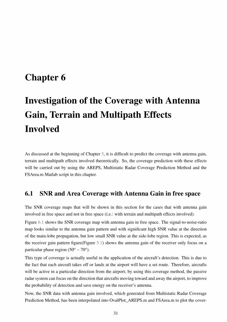
6.1 SNR coverage contours at 5000m altitude in free space with antenna gain involved . 32

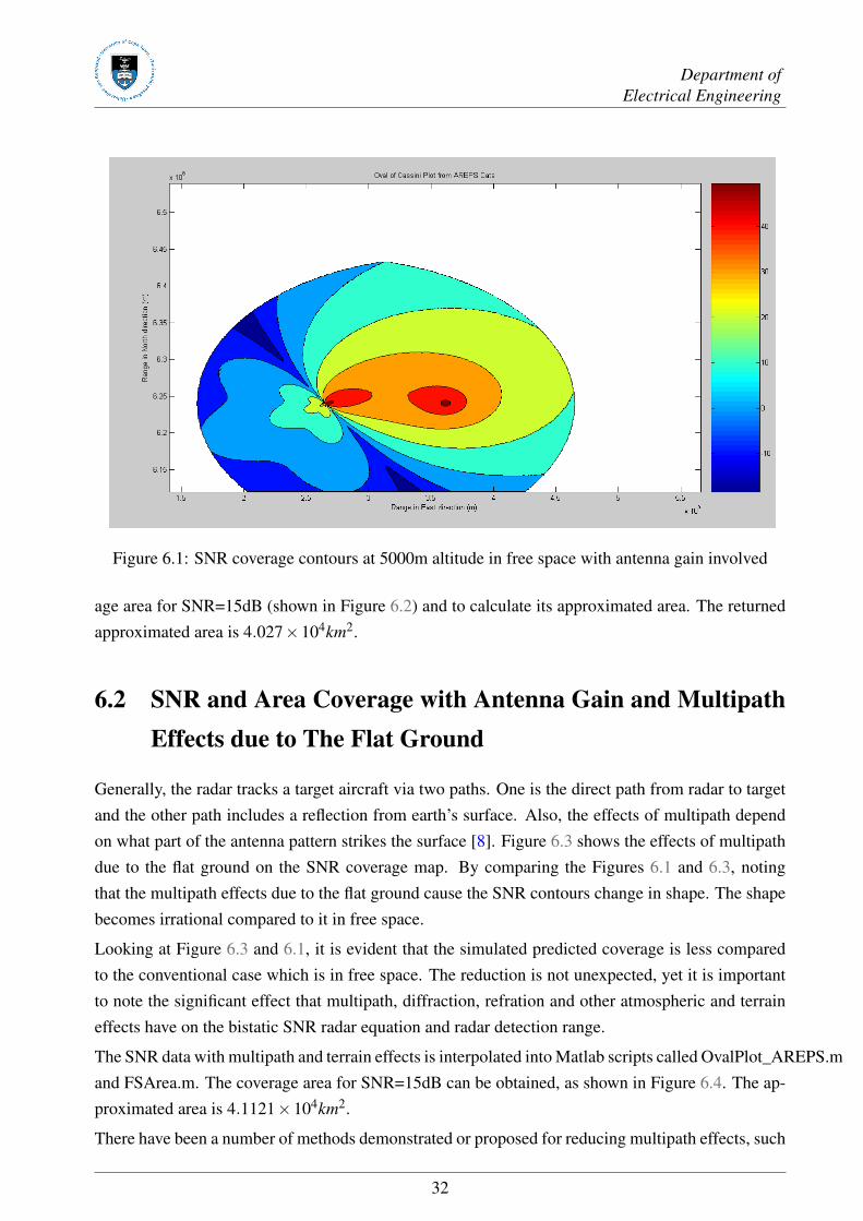
6.2 Oval of Cassini plot for SNR=15dB at 5000m altitude in free space with antennagain involved . . . . . . . . . . . . . . . . . . . . . . . . . . . . . . . . . . . . . . 33

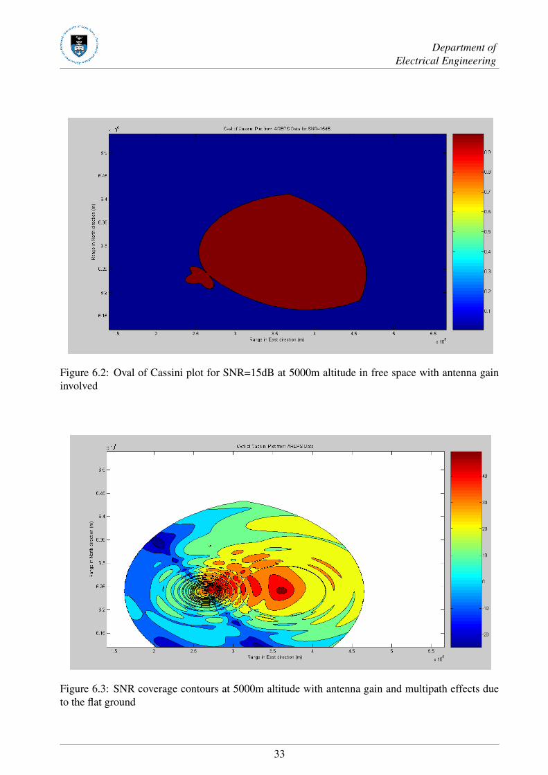
6.3 SNR coverage contours at 5000m altitude with antenna gain and multipath effectsdue to the flat ground . . . . . . . . . . . . . . . . . . . . . . . . . . . . . . . . . . 33

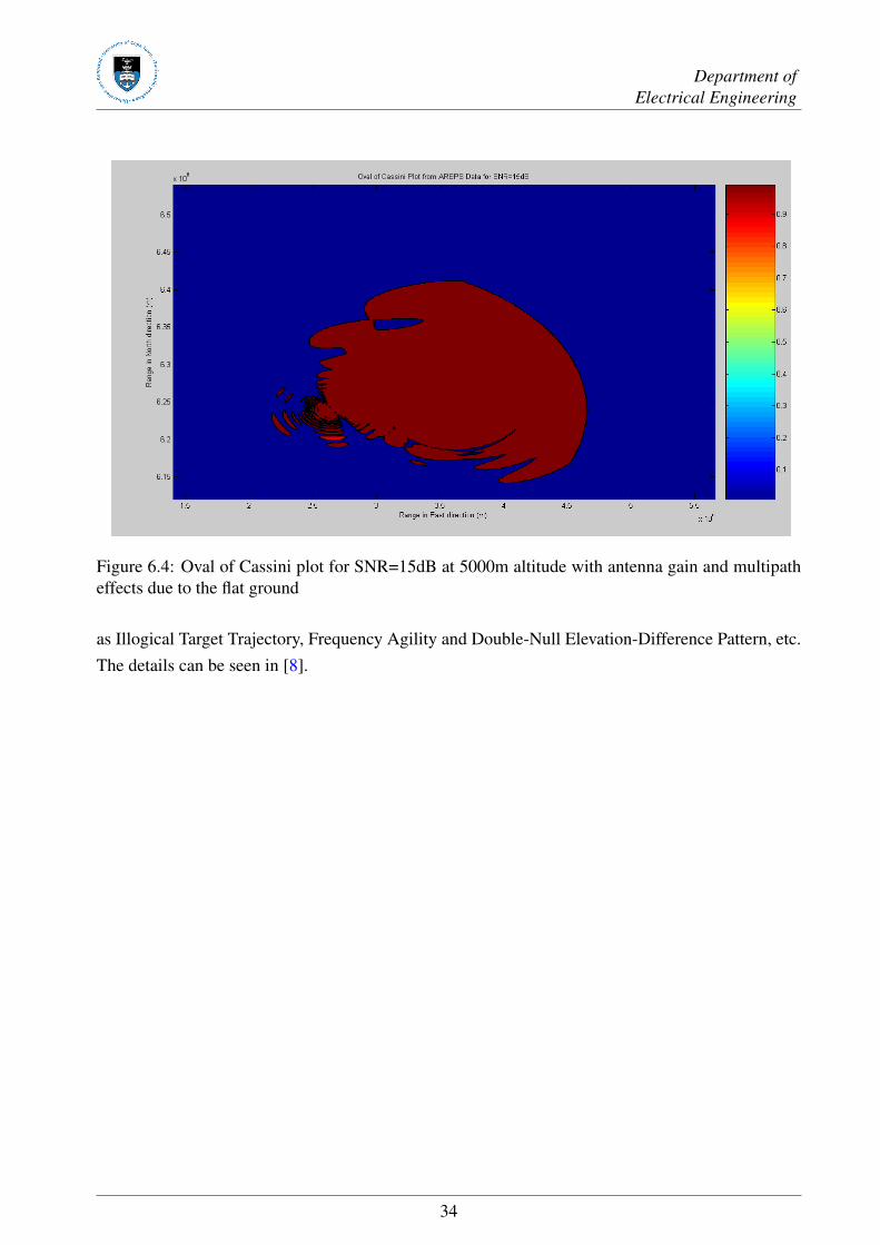
6.4 Oval of Cassini plot for SNR=15dB at 5000m altitude with antenna gain and multi-path effects due to the flat ground . . . . . . . . . . . . . . . . . . . . . . . . . . . . 34

7.1 SNR coverage contours at 1600m altitude with antenna gain and multipath effectsdue to the flat ground . . . . . . . . . . . . . . . . . . . . . . . . . . . . . . . . . . 35

vii


7.2 Oval of Cassini plot for SNR=15dB at 1600m altitude with antenna gain and multi-path effects due to the flat ground . . . . . . . . . . . . . . . . . . . . . . . . . . . . 36

8.1 Diagram for a standard one transmitter & two receivers passive radar system . . . . 38

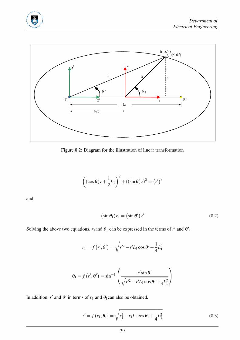
8.2 Diagram for the illustration of linear transformation . . . . . . . . . . . . . . . . . . 39

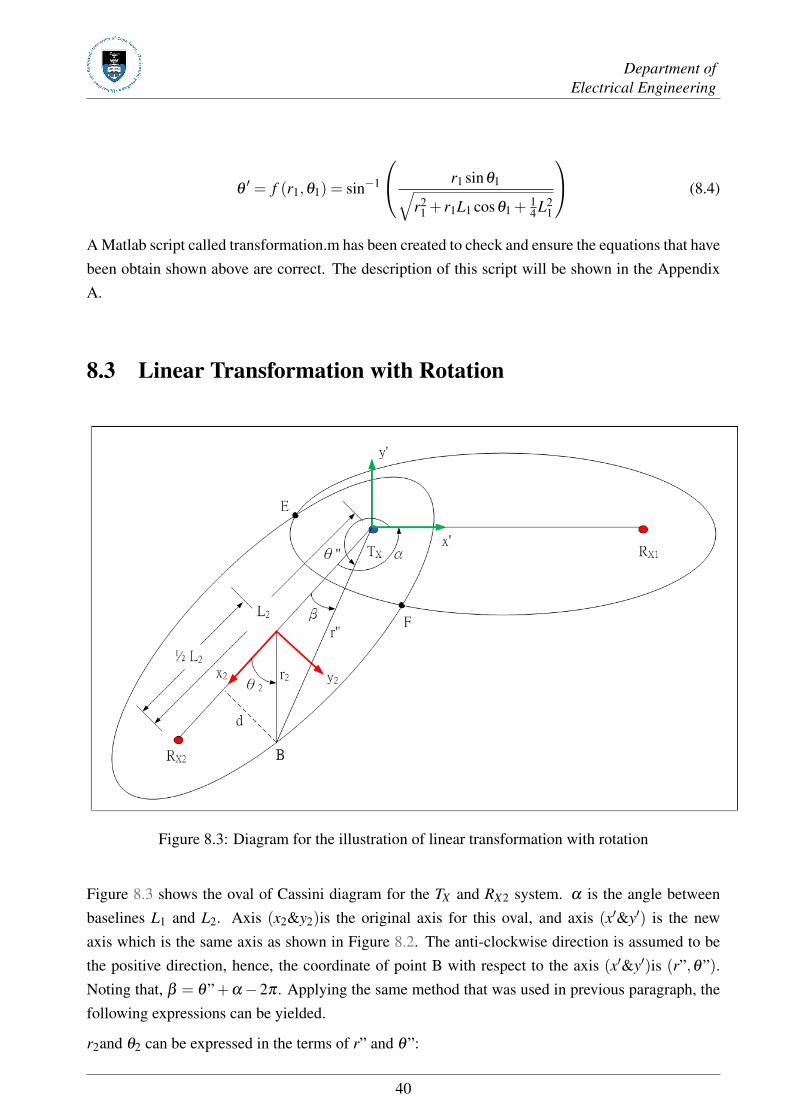
8.3 Diagram for the illustration of linear transformation with rotation . . . . . . . . . . . 40

8.4 Plot of the area of intersection for two ovals of Cassini . . . . . . . . . . . . . . . . 43

viii

List of Symbols

L — Baseline of the passive radar systemT x — TransmitterRx — ReceiverC — Bistatic angleαT — Transmitter look angleαR — Receiver look angleRT — Transmitter-to-target rangeRR — Receiver-to-target rangePT — Transmitted powerGT — Gain of the transmitter’s antennaGR — Gain of the receiver’s antennaλ — WavelengthσB — Bistatic radar target cross section area (target RCS)FT — Transmitter pattern propagation factorFR — Receiver pattern propagation factork — Boltzman’s constantTS — Receiver total noise temperatureBn — Receiver noise bandwidth( S

N

)min — Signal-to-noise ratio (SNR) needed for detection

LT — Losses in transmitterLR — Losses in receiverκ — Bistatic maximum range productσM — Monostatic radar target cross section area (target RCS)LM — Target range for monostatic radar systemF′T — Transmitter propagation factor

F′R — Receiver propagation factor

fT — Transmitter’s antenna pattern factorfR — Receiver’s antenna pattern factorK — Bistatic radar constant

ix


A — Amplitude of the sine waveI0 — Modified Bessel function of zero orderZ — ArgumentVT — ThresholdPd — Probability of detectionPf a — Probability of a false alarmψ0 — Mean square value of the noise voltageTf a — False alarm timeB — IF bandwidthAB1 — Coverage area for cosite regionAB2 — Coverage area for non-cosite regionAC — Common coverage arearT — Radius of the transmitter’s coverage arearR — Radius of the receiver’s coverage areaht — Target altitude (km)hT — Altitude of the transmitter antenna (km)hR — Altitude of the receiver antenna (km)c — Speed of lightf — Frequencyα — The angle between two baselines

x

Nomenclature

PCL—Passive Coherent Location

FM—Frequency modulated

AREPS—Advanced Refractive Effects Prediction System

APM—Advanced Propagation Model

CW—Continuous wave

OTH-B—Over-the-horizon-back-scatter

AOA—Angle of arrival

SNR—Signal-to-noise power ratio

RCS—Target cross section area

LOS—Light-of-sight

Azimuth—Angle in a horizontal plane, relative to a fixed reference, usually north or the longitudinalreference axis of the aircraft or satellite.

Beamwidth—The angular width of a slice through the mainlobe of the radiation pattern of an an-tenna in the horizontal, vertical or other plane.

Doppler frequency—A shift in the radio frequency of the return from a target or other object as aresult of the object’s radial motion relative to the radar.

Range—The radial distance from a radar to a target.

xi

Chapter 1

Introduction

1.1 Background

The defining property of bistatic radar, is the transmitter and receiver are not co-located. This simplymeans the fact that the transmitter and receiver are not located at the same position in bistatic radarsystem. A Passive Coherent Location (PCL) system (also called Passive radar) is a special case ofa bistatic radar and, more generally, multistatic radar, which is the case where the transmitters arenon-cooperative [4].

Passive radars or Passive Coherent Location systems encompass a class of radar systems that detectand track objects by processing reception from non-cooperative sources of illumination in the en-vironment, such as commercial broadcast systems such as television and radio and are commonlyreferred to as transmitters of opportunity.

PCL system does not contain transmitters (thus the term passive) but uses other emitters as trans-mitters [6], thus the achievable coverage depends not only on the transmitted power but also on theposition of the receivers as well. Therefore, the optimisation of the receiver site becomes a veryimportant issue in achieving maximum coverage in the passive radar system. This also emphasisesthe importance of receiver location information.

1.2 Objectives

The objectives of this thesis are:

• To investigate the use of the Advanced Refractive Effects Prediction System (AREPS) whichdeveloped by US Navy.

• To investigate the use of the Multistatic Radar Coverage Prediction Method which developedby Radar Remote Sensing Group in UCT (This method is based on the propagation loss data

1


which generated from AREPS).

• To investigate the relationship between coverage area and baseline (L)

• To validate the Multistatic Radar Coverage Prediction Method in the aspects of Oval of Cassiniand coverage area with theoretical predictions which are based on theoretical equations.

• To minimise the intersection area for a one transmitter and two receivers case in order toachieve maximum area of coverage.

• To investigate the effects of terrain and multipath in the passive radar coverage.

• To optimise the location of passive radar receiver in order to achieve maximum coverage ofaircraft moving around Cape Town International Airport.

These objectives are in essence quite broad, allowing for a variety of methods and techniques to beinvestigated and used. Yet, due to the broad nature of these objectives, the methods of the investiga-tions and analyses in each chapter will be clearly stated.

1.3 Plan of Development

Chapter 1 forms the introduction to this thesis. The background to this topic is discussed and ob-jectives of this project are presented here.

Chapter 2 is the literary review and presents various factors and information necessary and relatedto this thesis topic. The following topics will form the core to the literature review: The overviewof the bistatic radar, including its definition, advantages & disadvantages and classification, is beingdiscussed. This will be followed by a general description of passive radar. Within this descrip-tion, brief history, typical illuminations and advantages & disadvantages of passive radar will bereviewed. Fundamental theories of bistatic radar, such as coordinate system, geometry, range re-lationship, probabilities of detection & false alarm and target coverage, will also be discussed. Abrief description of APM & AREPS will be introduced. Finally, a Multistatic Radar Coverage Pre-diction Method which based on the interpolation of the propagation data from AREPS with Matlabpresented by Gunther Lange will be discussed briefly at the end of this chapter.

Chapter 3 will introduce a detailed criterion of this project. A list of limitations and assumptionshave been set-up before starting the investigation of this topic.

Chapter 4 The investigation of the relationship between SNR, baseline and coverage area, whichbased on the theoretical equations of bistatic radar, will be presented in this chapter. A mathematical

2


calculation for the maximum length of the baseline that will ensure the desired SNR falls within thecosite region in a given passive radar has been shown. Matlab will be used to plot and show therelationship between the baseline and coverage area.

Chapter 5 focuses on the coverage prediction without antenna gain involved in free space. Thereason for limiting the theoretical coverage prediction without antenna gain involved and within thefree space has been illustrated. This will be followed by the theoretical prediction of oval of Cassiniand coverage area based on the theoretical equations. Matlab has been used to plot the theoreticaloval of Cassini for SNR=15dB in our particular passive radar system. Thereafter, a Matlab scriptcalled FSArea.m has been created to calculate the approximated coverage area for a desired oval ofCassini, based on the SNR data generated from Multistatic Radar Coverage Prediction Method. Acomparison between the theoretical prediction and simulated results have been made on the SNRcoverage map and the coverage area.

The purpose of Chapter 6 is to investigate of the effects of the antenna gain, multipath and terrain onthe passive radar coverage. SNR coverage maps have been plotted by using Multistatic Radar Cov-erage Prediction Method. A Matlab script called OvalPlot_AREPS.m is used to plot the coveragearea for the desired SNR (15dB), hence, coverage with these effects involved can be viewed visually.

Chapter 7 has been designed to investigate the coverage with the change in altitude. The altitudethat being investigate is at 1600m. By using the Matlab script called FSArea.m, the approximatedarea can be calculated, and this value will be compared to the approximated area at 5000m. Bycomparing these two values of coverage, it verifies that the coverage will be less at low altitude asthe effects of multipath and terrain will be lessened at high altitude.

Chapter 8 investigates the coverage area in an one transmitter and two receivers passive radarsystem. The method of tackling this problem has been discussed at the beginning of this chap-ter. The mathematical calculation used to achieve linear transformation and linear transformationwith rotation of the axis in the polar coordinate, has also been shown. A Matlab script calledOvalPlot_transfo_coordinate.m has been created to simulate and plot the area of intersection basedon the expressions that have been shown in this chapter. The suggestion of finding the area of inter-section for two ovals has also been provided.

3

Chapter 2

Literature Review

The following review of literature was done on subjects that relate to or affect the subject of theproject undertaken. An overview of passive radar system will be outlined in the following few para-graphs. Bistatic radar fundamentals essential to the topic of the project will be discussed. AREPSand Multistatic Radar Coverage Prediction Method will also be introduced briefly at the end of thischapter.

2.1 Overview of Bistatic Radar

Bistatic radar is defined as a radar that uses antennas at different locations for transmission andreception. This means the fact that the transmitter and receiver are not co-located in the bistaticradar system. Recently, there are different versions of definition of bistatic radar as a conventionalbistatic radar system does not specify how far the transmitting and receiving sites must be sepa-rated. Attempts have been made to quantify this separation by Skolnik and Blake. Both Blake’sdirection-distance and Skolnik’s path separation criteria apply to all bistatic configuration. The pur-pose for establishing these separation criteria is simply to distinguish special types of radar, such ascontinuous wave (CW) and over-the-horizon-back-scatter (OTH-B) radars [11].

2.1.1 Advantages and Disadvantages of Bistatic Radar System

The principal advantages of Bistatic and Multistatic radar include [9]:

• Lower procurement and maintenance costs (if using a third party’s transmitter, such as passiveradar system)

• Operation without a frequency clearance (if using a third party’s transmitter, such as passiveradar system)

4


• Covert operation of the receiver

• Increased resilience to electronic countermeasure as waveform being used and receiver loca-tion are potentially unknown

• Possible enhanced radar cross section of the target due to geometrical effects

The principal disadvantages of bistatic and multistatic radar include:

• System complexity

• Costs of providing communication between sites

• Lack of control over transmitter (if exploiting a third party transmitter)

• Harder to deploy

• Reduced low-level coverage due to the need for line-of-sight from several locations

2.1.2 Specific Classes of Bistatic Radar

Generally, there are four specific classes of bistatic radar. These four specific classes include [9]:

1. Pseudo-monostatic radar has the angle which subtended between transmitter, target and re-ceiver (the bistatic angle) is close to zero.

2. Forward scatter radar is the bistatic radar that be designed to operate in a fence-like con-figuration, detecting targets which pass between the transmitter and receiver, with the bistaticangle near 180 degrees.

3. Multistatic radar is one in which there are at least three components - for example, onereceiver and two transmitter, or two receivers and one transmitter, or multiple receivers andmultiple transmitters. It is a generalisation of the bistatic radar system, with one or morereceivers processing returns from one or more geographically separated transmitters.

4. Passive radar is a bistatic or multistatic radar that exploits non-radar transmitters of oppor-tunity. This radar system is also known as Passive Coherent Location (PCL) system. Passiveradar is the specific type of the bistatic radar that being investigated in this project.

5


2.2 Overview of Passive Radar

A passive radar is a special case of a bistatic radar [4].In a passive radar system, there is no dedicatedtransmitter. Instead, the receiver uses third-party transmitters in the environment, and measures thetime difference of arrival between the signal arriving directly from the transmitter and the signalarriving via reflection from the object. So, the bistatic range of the object can be calculated. Inaddition to bistatic range, a passive radar will typically also measure the bistatic Doppler shift of theecho and also its direction of arrival. Therefore, the location, heading and speed of the object can becalculated. Multiple transmitters and/or receivers will be introduced to make different independentmeasurements in order to improve the final track accuracy and the area of coverage [10].

2.2.1 Brief History of Passive Radar

The concept of passive radar detection - using reflected ambient radio signals emanating from adistant transmitter - is not now. The first radar experiments in the United Kingdom in 1935 byRobert Watson - Watt demonstrated the principle of radar by detecting a Handley Page Heyfordbomber at a distance of 12 km Using the BBC shortwave transmitter at Daventry.

Early radars were all bistatic because the technology to enable an antenna to be switched fromtransmit to receiver mode had not been developed. Thus many countries were using bistatic systemsin air defence network during the early 1930s.

The Germans used a passive bistatic system during World War II. This system, call the KleineHeidelberg device, was located at Ostend and operated as a bistatic receiver, using the British ChainHome radars as non-cooperative illuminators, to detect aircraft over the southern part of North Sea.

Bistatic radar systems gave way to monostatic systems with the development of the synchronizerin 1936 since the monostatic systems were much easier to implement. In the early 1950s, bistaticsystems were considered again when some interesting properties of the scattered radar energy werediscovered, indeed the term “bistatic” was first used by Seigel in 1955 in his report describing theseproperties.

Experiments in the United States led to the deployment of a bistatic system in North AmericanDistant Early Warning Line around 1955.

The rise of cheap computing power and digital receiver technology in the 1980s led to a resurgence ofinterest in passive radar technology. For the first time, these allowed designers to apply digital signalprocessing techniques to exploit a variety of broadcast signals and to use cross-correlation techniquesto achieve sufficient signal processing gain to detect targets and estimated their bistatic range andDoppler shift. Classified programmes existed in several nations, but the first announcement of acommercial system was by Lockheed-Martin Mission Systems in 1998, with the commercial launchof the Silent Sentru system, that exploited FM radio and analogue television transmitters [10].

6


2.2.2 Typical Illumination of Passive Radar

Passive radar systems have been developed the exploit the following sources of illumination [10]:

• Analog television signals

• FM radio signals

• GSM base stations

• Digital audio broadcasting

• Digital video broadcasting

• Terrestrial High-definition television transmitters in North America

Satellite signals have generally been found to be inadequate for passive radar use: either because thepowers are too low, or because the orbits of the satellites are such that illumination is too infrequent.

2.2.3 Advantages and Disadvantages of Passive Radar System

The advantages of passive radar system over conventional bistatic radar system are [10]:

• Physically small and hence easily deployed in places where conventional radars cannot be

• Capabilities against stealth aircraft due to the frequency bands and multistatic geometries em-ployed

• Rapid updated, typically once a second

• Difficulty of jamming

• Resilience to anti-radiation missiles

The disadvantages of passive radar system over conventional bistatic radar system are [10]:

• Immaturity

• Reliance on third-party illuminators

• Complexity of deployment

• 2D operation

7


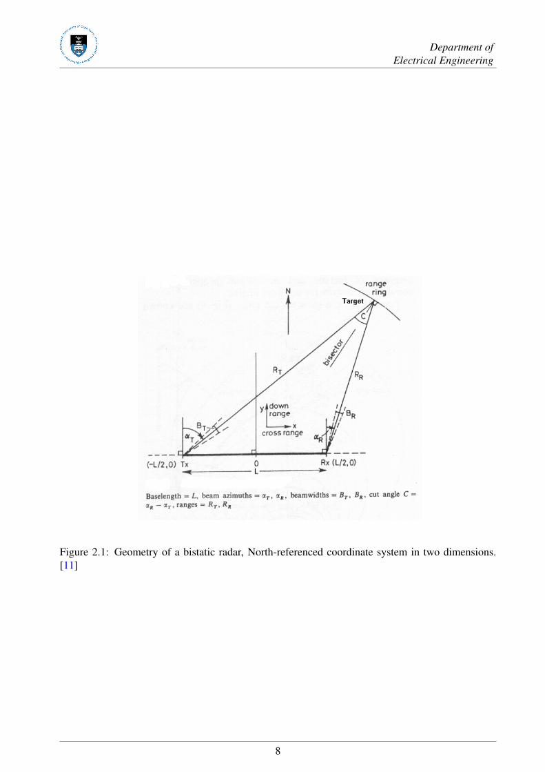
Figure 2.1: Geometry of a bistatic radar, North-referenced coordinate system in two dimensions.[11]

8


2.3 Coordinate Systems and Geometry

Due to the separate positioning locations of the transmitter and the receiver, the coordinate systemand the geometry of a bistatic radar system can be complex in a way.

The coordinate system used to describe the geometry will be in a two dimensional case, a northreferenced coordinate system which shown on Figure 2.1. The bistatic plane, is the plane on whichthe transmitter (Tx), receiver (Rx) and the target (on the edge of the range ring) lie. On this particularplane, the ellipse with its foci at Tx and Rx is also presented (the range ring). This ellipse has itsmidpoint located on the midpoint of the transmitter and receiver stations.

All the ellipses have a common transmitting and receiving site foci, and therefore a common baseline(L). The bistatic system which is shown in Figure 2.1, is known as the bistatic triangle.

As shown on the Figure 2.1, the baseline (L) is the distance between the transmitter (Tx) and receiver(Rx). The distance from the transmitter to the target is defined as RT and from the receiver to thetarget is RR.

The bistatic angle is C, or β , which is also known as the cut angle, which is the angle between thetransmitter and the receiver, with the vertex at the target. The transmitter look angle is αT and thereceiver look angle is αR. Counter clockwise direction will be taken as positive for the look angles.They are also known as the angle of arrival (AOA) [11]. Also, note that:

αT +αR = C = β (2.1)

In a general case, the bistatic system works the same, irrespective of whether the target lies above orbelow the baseline. This is due to its symmetrical nature of their geometry.

2.4 Range Relationships

The bistatic range equation is similar in form to the monostatic range equation and is derived in asimilar process. The effect of the propagation factors on the range will be mentioned briefly and theovals of Cassini (SNR contours) will also be discussed in detail later in this section.

2.4.1 Bistatic Radar Range Equations

The range equations for a bistatic radar are derived in a manner that exactly the same way in themonostatic radar case. The derivation of these equations can be found in [7]. With this analog, thebistatic radar maximum range equation, from Willis [11], is shown below.

(RT RR)max =

[PT GT GRλ 2σBF2

T F2R

(4π)3 kTsBn( S

N

)min LT LR

] 12

(2.2)

9


or

(RT RR)max = κ (2.3)

where

RT = transmitter-to-target range

RR = receiver-to-target range

PT = transmitted power

GT = gain of the transmitter’s antenna

GR = gain of the receiver’s antenna

λ = wavelength

σB = bistatic radar target cross section area (target RCS)

FT = transmitter pattern propagation factor

FR= receiver pattern propagation factor

k = Boltzman’s constant

TS= receiver total noise temperature

Bn= receiver noise bandwidth( SN

)min = signal-to-noise ratio (SNR) needed for detection

LT = losses in transmitter (cables, signal processing, etc.)

LR = losses in receiver (cables, signal processing, etc.)

κ = bistatic maximum range product

The FM radio broadcast antenna is assumed to be omni-directional, and therefore 0dBi gain can beassumed. Also, for calculation purposes, we first assume the pattern propagation factor FR = FT =1. For this bistatic radar maximum range equation to be reduced to monostatic case, the followingvariables needs to be changed [11]:

1. σB = σM

2. LT LR = LM

3. R2T R2

R = (RT RR)2 =(R2

M)2= R4

M

Note that (RM)max=√

κ . The term√

κ is sometimes called the equivalent monostatic range, whichoccurs when the transmitting and receiving sites are located at the same location [5].

10


2.4.2 Pattern Propagation Factors

The transmitting and receiving pattern propagation factors, FT and FR, are the product of the prop-agation factor (F

′T and F

′R) and antenna pattern factor ( fT and fR) respectively. The pattern propa-

gation factors take into account the gains of the transmit and receive antennas as a pointing angle.The losses in the signal (atmospheric, absorption, etc) are also taken into account while propagatingthrough the atmosphere. More about the pattern propagation factors can be found in [11].

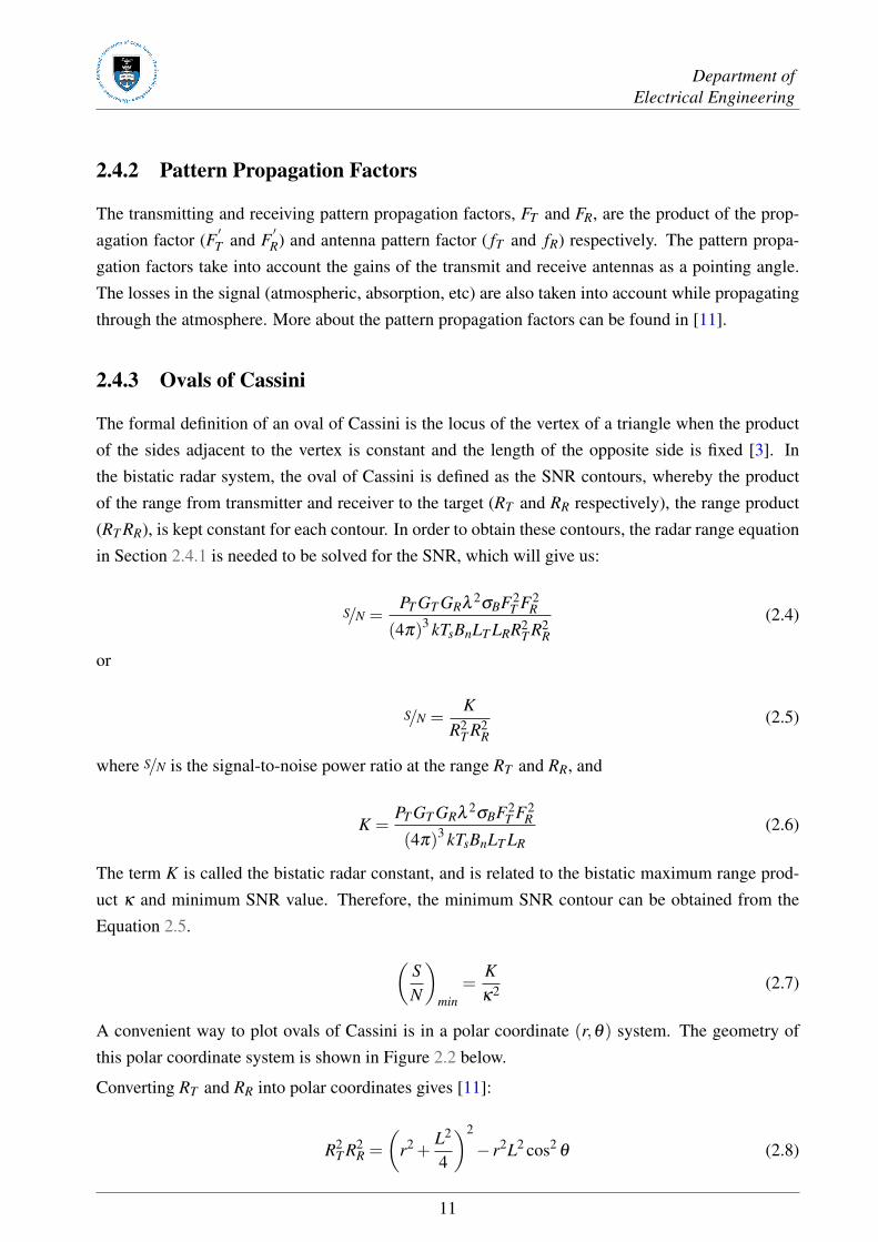
2.4.3 Ovals of Cassini

The formal definition of an oval of Cassini is the locus of the vertex of a triangle when the productof the sides adjacent to the vertex is constant and the length of the opposite side is fixed [3]. Inthe bistatic radar system, the oval of Cassini is defined as the SNR contours, whereby the productof the range from transmitter and receiver to the target (RT and RR respectively), the range product(RT RR), is kept constant for each contour. In order to obtain these contours, the radar range equationin Section 2.4.1 is needed to be solved for the SNR, which will give us:

S/N =PT GT GRλ 2σBF2

T F2R

(4π)3 kTsBnLT LRR2T R2

R

(2.4)

or

S/N =K

R2T R2

R(2.5)

where S/N is the signal-to-noise power ratio at the range RT and RR, and

K =PT GT GRλ 2σBF2

T F2R

(4π)3 kTsBnLT LR(2.6)

The term K is called the bistatic radar constant, and is related to the bistatic maximum range prod-uct κ and minimum SNR value. Therefore, the minimum SNR contour can be obtained from theEquation 2.5. (

SN

)min

=Kκ2 (2.7)

A convenient way to plot ovals of Cassini is in a polar coordinate (r,θ) system. The geometry ofthis polar coordinate system is shown in Figure 2.2 below.

Converting RT and RR into polar coordinates gives [11]:

R2T R2

R =(

r2 +L2

4

)2

− r2L2 cos2θ (2.8)

11


Figure 2.2: Geometry for converting North-referenced coordinates into polar coordinates (r,θ). [11]

Substituting Equation 2.8 into Equation 2.5 gives:

S/N =K(

r2 + L2

4

)2− r2L2 cos2 θ

(2.9)

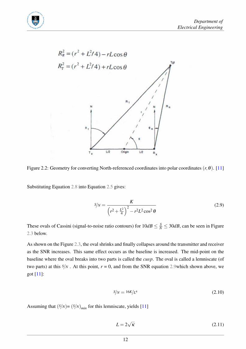
These ovals of Cassini (signal-to-noise ratio contours) for 10dB ≤ SN ≤ 30dB, can be seen in Figure

2.3 below.

As shown on the Figure 2.3, the oval shrinks and finally collapses around the transmitter and receiveras the SNR increases. This same effect occurs as the baseline is increased. The mid-point on thebaseline where the oval breaks into two parts is called the cusp. The oval is called a lemniscate (oftwo parts) at this S/N . At this point, r = 0, and from the SNR equation 2.9which shown above, wegot [11]:

S/N = 16K/L4 (2.10)

Assuming that (S/N)= (S/N)min for this lemniscate, yields [11]

L = 2√

κ (2.11)

12


Figure 2.3: Contours of a constant SNR - ovals of Cassini. [11]

2.4.4 Operating Regions

From the equations in Section 2.4.3, three main operating regions can be defined [11], namely:

1. The receiver centred region - occurs when L> 2√

κ and RT � RR, hence the oval breaks intotwo parts.

2. The transmitter centred region - occurs when L> 2√

κ and RT � RR, hence the oval breaksinto two parts.

3. The cosite region - occurs when L< 2√

κ , therefore the oval remains single (oval does notdevelop a cusp or break into two parts, refer to Figure 2.3).

2.5 Probabilities of Detection and False Alarm

A specific probability of detection and probability of false alarm is required to achieve minimumsignal-to-noise ratio (

( SN

)min, shown in Section 2.4.1 and 2.4.3). From Equation 2.7 above, the

minimum signal-to-noise ratio is needed in order to calculate the bistatic maximum range product (κ)for a given bistatic constant,K [8], i.e.: given basic information of the specific bistatic radar systemsuch as the transmitted power and gain of transmitter’s & receiver’s antenna, etc (see Equation 2.6for details).

13


2.5.1 Probability of Detection

Now, let’s consider an echo signal represented as a sinewave of amplitude A along with Gaussiannoise at the input of the envelope detector. The probability density function of the envelope R at thevideo output is given by Rice probability density function,

ps (R) =Rψ0

exp(−R2 +A2

2ψ0

)I0

(RAψ0

)(2.12)

where I0 is the modified Bessel function of zero order and argument Z. The probability of detectingthe signal is the probability that the envelop R will exceed the threshold VT (set by the need to achievesome specific false-alarm time). Thus the probability of detection is

Pd =∫

∞

VT

ps (R)dR (2.13)

A series approximation method will be used to solve for Pd after substituting the Equation 2.12into Equation 2.13. Numerical and empirical methods can also be used [8]. The expression of theprobability of detection Pdin terms of SNR can be seen in [8]. Hence, the relationship between theprobability of detection and SNR & probability of false alarm can be shown in the Figure 3.1 inChapter 3.1.

2.5.2 Probability of False Alarm

The probability of a false alarm, Pf a, is denoted as

Pf a = exp(−−V 2

T2ψ0

)(2.14)

where VT is the voltage threshold and ψ0 is the mean square value of the noise voltage (mean noisepower).

or

Pf a =1

Tf aB(2.15)

where Tf a is the false alarm time and B is the IF bandwidth.

The detailed derivation of the probability of false alarm equation can be seen in [8]. The false-alarmprobabilities of radars are generally quite small since a decision as to whether a target is present ornot is made every 1/B second. The bandwidth B is usually large, so there are many opportunitiesduring one second for a false alarm to occur. If the threshold is set slightly higher than required andmaintained stable, there is little likelihood of false alarms due to thermal noise. In practice, false

14


alarms are more likely to occur from clutter echoes (ground, sea, weather, birds, and insects) thatenter the radar and are large enough to cross the threshold [8].

2.6 Target Coverage

Coverage is an important factor in bistatic radars, and this can be defined as the area on the bistaticplane whereby the target is visible to both the transmitter and receiver. Bistatic coverage is detectedin two ways [11]:

1. Detection-constrained coverage. This type of coverage is constrained by the maximum rangeproduct of the oval of Cassini (RT RR)max. When the oval of Cassini encapsulates both thetransmitter and the receiver (the cosite region), the coverage area can be approximated by:

AB1 ≈ πκ

{1−(

164

)(L4

κ2

)−(

316384

)(L8

κ4

)}(2.16)

But when the oval of Cassini surrounds the transmitter and receiver with two separate circles,the coverage area is approximated by:

AB2 ≈(

2πκ2

L2

)(1+

2κ2

L4 +12κ4

L8 +100κ6

L12

)(2.17)

In a monostatic case (i.e.: transmitter and receiver locate at the same position), therefore, L =0, and the coverage area for the monostatic radar becomes:

AM = πκ = π (RM)2max (2.18)

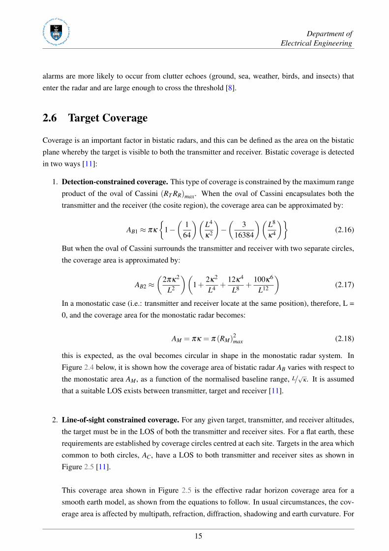
this is expected, as the oval becomes circular in shape in the monostatic radar system. InFigure 2.4 below, it is shown how the coverage area of bistatic radar AB varies with respect tothe monostatic area AM, as a function of the normalised baseline range, L/

√κ. It is assumed

that a suitable LOS exists between transmitter, target and receiver [11].

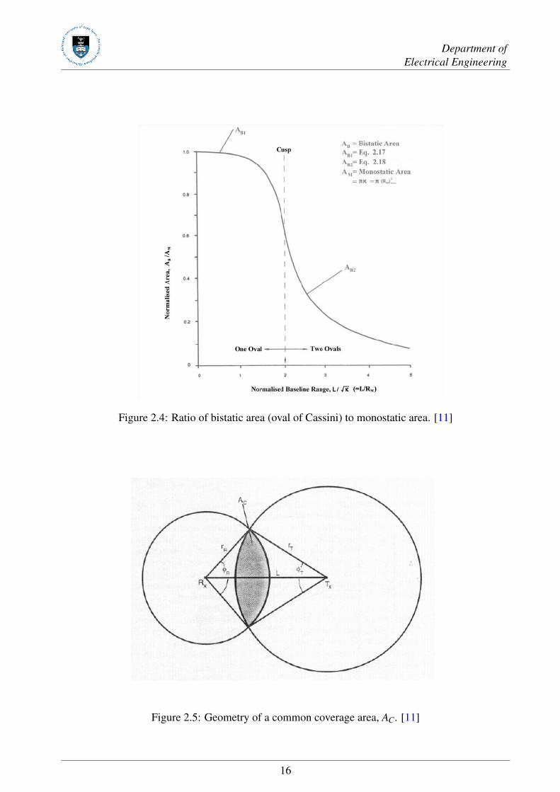
2. Line-of-sight constrained coverage. For any given target, transmitter, and receiver altitudes,the target must be in the LOS of both the transmitter and receiver sites. For a flat earth, theserequirements are established by coverage circles centred at each site. Targets in the area whichcommon to both circles, AC, have a LOS to both transmitter and receiver sites as shown inFigure 2.5 [11].

This coverage area shown in Figure 2.5 is the effective radar horizon coverage area for asmooth earth model, as shown from the equations to follow. In usual circumstances, the cov-erage area is affected by multipath, refraction, diffraction, shadowing and earth curvature. For

15


Figure 2.4: Ratio of bistatic area (oval of Cassini) to monostatic area. [11]

Figure 2.5: Geometry of a common coverage area, AC. [11]

16


a 43 earth model, and ignoring multipath lobing, the radius of the coverage areas can be ap-

proximated in kilometres by the following equations [11].

rT ∝ 130(√√

ht +√

hT

)(2.19)

rR ∝ 130(√√

ht +√

hR

)(2.20)

whererT = radius of the transmitter’s coverage arearR = radius of the receiver’s coverage areaht = target altitude (km)hT = altitude of the transmitter antenna (km)hR = altitude of the receiver antenna (km)These derivation of these equations can be found in Willis [11]. The common area betweenthe transmitter and the receiver is the intersection area between the two circles.

AC =12[r2

R (φR− sinφR)+ r2T (φT − sinφT )

](2.21)

whereφR = 2arccos

(r2

R−r2T +L2

2rRL

)φT = 2arccos

(r2

T−r2R+L2

2rT L

)These equations are valid for L + rR > rT > L− rR or L + rT > rR > L− rT . Whenever theright-hand side of either inequality is not satisfied such that rT + rR ≤ L then AC = 0. Thismeans that the coverage areas of the transmitter and receiver do not intersect. When the left-hand side of the first inequality, AC = πr2

T . This is because the receiver’s coverage includes thetransmitter’s coverage completely, and vice-versa.

For our particular system, the detection-constrainted coverage method will be used to investigate thecoverage of our specific passive radar system. Our coverages area is also mainly dependent on ourantenna system, i.e.: the information of transmitter and receiver, can be seen in Chapter 3.3.

2.7 Advanced Propagation Model and AREPS

Advanced Refractive Effects Prediction System, is also called AREPS, which was developed in2003 by the Space and Naval Warfare Systems centre of US Navy at San Diego [2]. The AdvancedPropagation Model (APM) is the propagation model used within AREPS [1]. APM is a hybrid rayoptics and parabolic equation propagation model, functional for all frequencies between 2MHz and

17


57GHz. The advantageous feature of the APM and AREPS software is the propagation factor, F ,can be computed from them, given relevant regional terrain and atmospheric data.

The goal in the development of APM was to create an all-encompassing propagation model for theincorporation into the U.S. military’s electromagnetic performance assessment systems. In additionto its use by the U.S. military and other U.S. government agencies, APM and AREPS are well-provenand widely used by academic institutions and foreign agencies across the world [4].

2.8 Multistatic Radar Coverage Prediction Method

Multistatic Radar Coverage Prediction Method, also called MRCPM in this report, is an accuratemodelling method that developed by the Radar Remote Sensing Group in University of Cape Town.It uses the propagation loss data generated by APM and captured from AREPS, to predict the signalpath loss among a transmitter, aircraft & a receiver and spatial coverage in the Passive CoherentLocation (PCL) system. The coverage plots which generated from this method, are in the form ofspatial signal-to-noise ratio (SNR) maps. These SNR maps can provide a visual means for determin-ing the radar detection range and coverage feasibility. The details of this prediction method can beseen in [4]. The best advantage of this method is the propagation loss data in a specific passive radarsystem which generated from AREPS, is converted into SNR data by this method. According to therelationship between the SNR, maximum range product (κ) and coverage area shown in previoussections, hence, it provides us a powerful tool to investigate the detection range and the optimisationof coverage in passive radar system.

18

Chapter 3

Project Criterion Setup

As the scope of the topic of this project is very broad, therefore, it is necessary to setup a set ofcriterion throughout the whole project execution. The detailed criterion setup for this project will bediscussed in this chapter.

3.1 Signal-to-noise ratio setup

Albersheim developed a simple empirical formula for the relationship between signal-to-noise ratio( S

N ), probability of detection (Pd) and probability of false alarm (Pf a), which is

S/N = A+0.12AB+1.7B (3.1)

where

A = ln[0.62/Pf a

]and B = ln [Pd/(1−Pd)]

Note that, the signal-to-noise ratio in the above equation is numerical, and not in dB; and ln is thenatural logarithm [8]. From the Equation 3.1 above, it shows the SNR depends on the values of theprobability of detection and false alarm. For the passive radar system that investigated in this project,supposes that the average time between false alarms is required to be 1.5 min, i.e.:Tf a= 1.5min. Andthe bandwidth of the IF is 100kHz, i.e.:B=100kHz. From the Equation 2.15, the probability of falsealarm can be obtained.

Pf a =1

Tf aB=

1(1.5×60)(100×103)

≈ 1.11×10−7

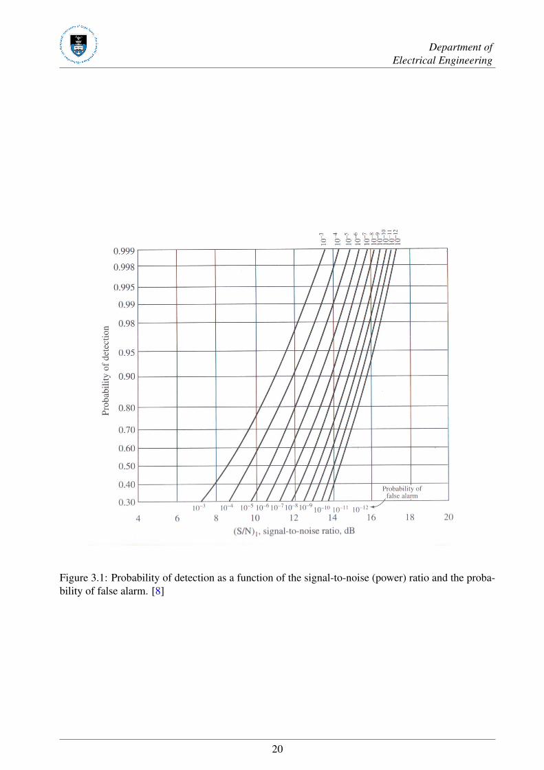
The relationship between SNR, Pf a and Pd can be shown in the Figure 3.1. This relationship figureshows for probability of false alarm equals to 1×10−7, signal-to-noise ratio of 12dB is required fora probability of detection of 0.50, 15dB for Pd = 0.99, and 15.75dB for Pd = 0.998. Thus, a change

19


Figure 3.1: Probability of detection as a function of the signal-to-noise (power) ratio and the proba-bility of false alarm. [8]

20


of 3dB can mean the difference between highly reliable detection (0.99) and marginal detection(0.5). This probability of false alarm curve has a significant change of probability of detectionbetween SNR of 11dB and 15dB. However, as the SNR increased more than 15dB, the probabilityof detection will only change very slightly as the increasing of the SNR, as shown in Figure 3.1.Also, a probability of detection of 0.99 can be considered as a highly reliable detection. Therefore,SNR = 15dB has been set as our desired (interesting) signal-to-noise ratio in our investigated radarsystem.

3.2 Altitude and Coverage Range Setup

The target altitude that is to be investigated is 5000m, as it is the standard height for an airportapproach. For avoiding the complexity, the transmitter and receiver can be assumed to be of thesame altitude. The reason for assuming this case is shown as following: for instance, if the LOSdistance between the transmitter and receiver is 120km, and their height difference is 60m. So,according to the Pythagorean theorem, the actual distance (surface distance) between the transmitter

and receiver will be: B =√

C2−A2 =√

(120×103)2−602 ≈ 119.999km. The surface distance isalmost same as the direct LOS distance, as the length of hypotenuse is much longer than the lengthof leg. Therefore, we can assume Tx and Rx are at the same altitude.

The range of investigation will cover all the area within 150km radius from the airport. The distancebetween transmitter and receiver (baseline length, L) will be limited within 150km in this project.The reason for setting up this criterion will be discussed in next chapter.

3.3 Passive Radar System Setup

In this project, specific transmitter and receiver have been chosen in order to conduct a better investi-gation on the coverage in the passive radar system practically. The chosen transmitter is Villiersdorptransmitter and the chosen receiver is Menzies receiver. The detailed information of the chosentransmitter and receiver is shown below:

[Transmitter information]

1. Tx Name = Villiersdorp

2. Tx Latitude [d,m,s,Hemi] = 33,58,9,S

3. Tx Longitude [d,m,s,Hemi] = 19,30,25,E

4. AREPS Tx Project Folder Name = VilliersdorpTx96.5

5. Frequency [MHz] = 96.5

21


6. Power [W] = 1000

7. Beamwidth start [0-359 deg] = 0

8. Beamwidth end [0-359 deg] = 359

9. Gain within beamwidth [dB] = 10

10. Gain outside beamwidth [dB] = -30

[Receiver Information]

1. Rx Name = Menzies

2. Rx Latitude [d,m,s,Hemi] = 33,57,31.16,S

3. Rx Longitude [d,m,s,Hemi] = 18,27,36.36,E

4. AREPS Rx Project Folder Name = MenziesRx96.5

5. Antenna Pattern [data file] = AntPat.mat

6. Rx Beamwidth start [0-359 deg] = 0

7. Rx Beamwidth end [0-359 deg] = 359

8. Pad receiver beamwidth [y/n] = n

9. Padded beamwidth [deg] = 5

10. Receiver Noise Figure Fn [dB] = 10

In addition, the surface distance between Villiersdorp transmitter and Menzies receiver is L =96.53km. The explanation of specific transmitter and receiver has to be chosen before investiga-tion of passive radar coverage is shown in the Chapter 3.4.

3.4 Bistatic Constant Setup

A bistatic constant, K, must be given in order to investigate the coverage area for a specific SNRin a passive radar system. Equations 2.16 and 2.17 shows the there is significant link between thecoverage area and the maximum range product κ . Also, the Equation 2.7 can be written as

κ2 =

K( SN

)min

(3.2)

22


or

κ =

√K( S

N

)min

(3.3)

For a given SNR, we need to specify the value of bistatic constant, K, to obtain the value for max-imum range product,κ . Therefore, bistatic constant (K) must be specified in order to calculate thecoverage area for a given SNR theoretically. Note that, from the bistatic constant equation shownin Equation 2.6, the bistatic constant depends on the specified information from the transmitter andreceiver. Different passive radar system or different combinations of transmitter and receiver willresult in different values of bistatic constant (K). This is the reason why transmitter and receiverneeds to be specified before starting to investigate passive radar coverage.

From the information shown in Chapter 3.3, the bistatic constant (K) without antenna gain can beobtained.

K =1000×1×1×

(3000965

)2×10×12×12

(4π)3×1.38×10−23×2900×1×1×1≈ 1.217×1021

Note that:

For a bistatic constant without antenna gain involves, GT = GR = 1. Wave length λ= cf = 3×108m/s

96.5×106Hz =3000965 m. The transmitter and receiver pattern propagation factor, FT = FR = 1. The losses in trans-

mitter and receiver, LT = LR = 1. The target cross section area is set to be 10m2. The receivernoise bandwidth in the equation which is the same as the SNR processing bandwidth as shown inthe information above. The total receiver noise temperature can be obtained from Ts = T0 + Te =T0 +(F−1)×T0 = 290+(10−1)×290 = 2900K.

23

Chapter 4

Investigation of The Relationship BetweenSNR, Baseline and Coverage Area

4.1 Relationship Between SNR and Baseline

As mentioned in Chapter 3.1, signal-to-noise ratio of 15dB is the desired SNR in this project. FromEquation 2.10 which shown in Chapter 2.4.3, it shows the SNR equation for the oval of Cassini justbreaks into two parts. This project will only interest the oval of Cassini which does not develop acusp. Therefore, for a given SNR, the maximum range of the baseline (L) which will not result theoval break into two parts, can be found from the Equation 2.10.

L =(

16KS/N

)1/4

≈ 511km

As specified in Chapter 3.2, the baseline for our system is limited to within 150km, which is muchsmaller than the maximum range of the baseline shown above, 511km. Therefore, it will make surethat the oval of Cassini (SNR contour) of SNR = 15dB will never break into two parts in our passiveradar system.

4.2 Relationship Between Coverage Area and Baseline

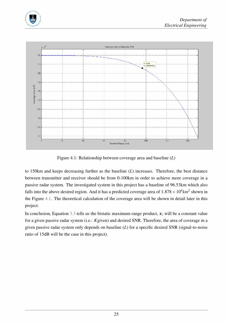
According to the Equation 3.3, bistatic maximum range product, κ , can be obtained from a givenpassive radar system (K given) and SNR. A Matlab script called Area_vs_Baseline_Plot.m has beencreated to plot and show different values of the coverage area for baseline (L) varies from 0 to 150kmbased on the Equation 2.16. This plot is shown in Figure 4.1.

Figure 4.1 shows the value of coverage area decreases as the length of baseline increases. Also,the curve only decreases gently from 0 to 100km, but starts decreasing dramatically from 100km

24


Figure 4.1: Relationship between coverage area and baseline (L)

to 150km and keeps decreasing further as the baseline (L) increases. Therefore, the best distancebetween transmitter and receiver should be from 0-100km in order to achieve more coverage in apassive radar system. The investigated system in this project has a baseline of 96.53km which alsofalls into the above desired region. And it has a predicted coverage area of 1.878×104km2 shown inthe Figure 4.1. The theoretical calculation of the coverage area will be shown in detail later in thisproject.

In conclusion, Equation 3.3 tells us the bistatic maximum range product, κ , will be a constant valuefor a given passive radar system (i.e.: Kgiven) and desired SNR. Therefore, the area of coverage in agiven passive radar system only depends on baseline (L) for a specific desired SNR (signal-to-noiseratio of 15dB will be the case in this project).

25

Chapter 5

Coverage Prediction Without Antenna GainInvolved in Free Space

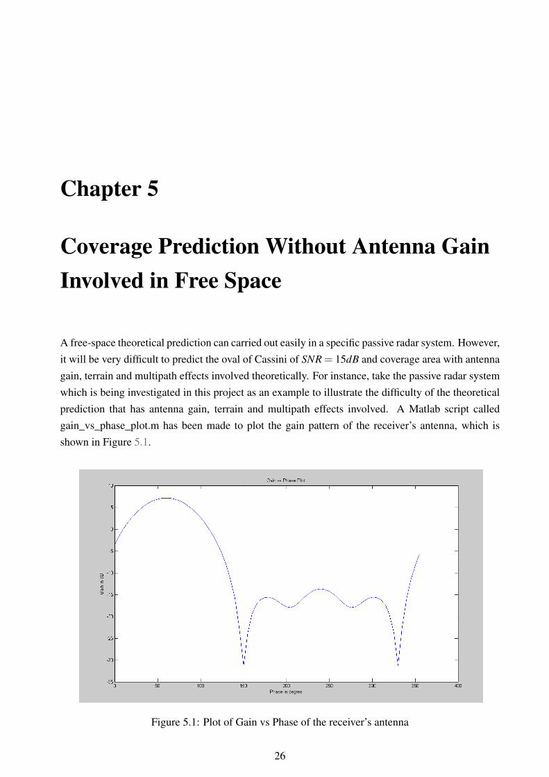
A free-space theoretical prediction can carried out easily in a specific passive radar system. However,it will be very difficult to predict the oval of Cassini of SNR = 15dB and coverage area with antennagain, terrain and multipath effects involved theoretically. For instance, take the passive radar systemwhich is being investigated in this project as an example to illustrate the difficulty of the theoreticalprediction that has antenna gain, terrain and multipath effects involved. A Matlab script calledgain_vs_phase_plot.m has been made to plot the gain pattern of the receiver’s antenna, which isshown in Figure 5.1.

Figure 5.1: Plot of Gain vs Phase of the receiver’s antenna

26


Figure 5.1 shows the gain of receiver’s antenna changes as the phase changes. The gain of receiver(GR) is not a constant value but a function of the phase. Hence, the value of the bistatic constant (K)will also change with the change of receiver gain (GR) according to the bistatic constant equation.Therefore, it is difficult to predict the theoretical coverage area with the antenna gain involved. Theeffects of terrain and multipath will result in change of the value of transmitter & receiver patternpropagation factors (FT & FR) in the bistatic constant equation, hence, results in changes of thebistatic constant value. This is the reason why theoretical prediction is very difficult to be achievedwith terrain and multipath effects involved.

5.1 Theoretical Prediction of Oval of Cassini and Coverage Area

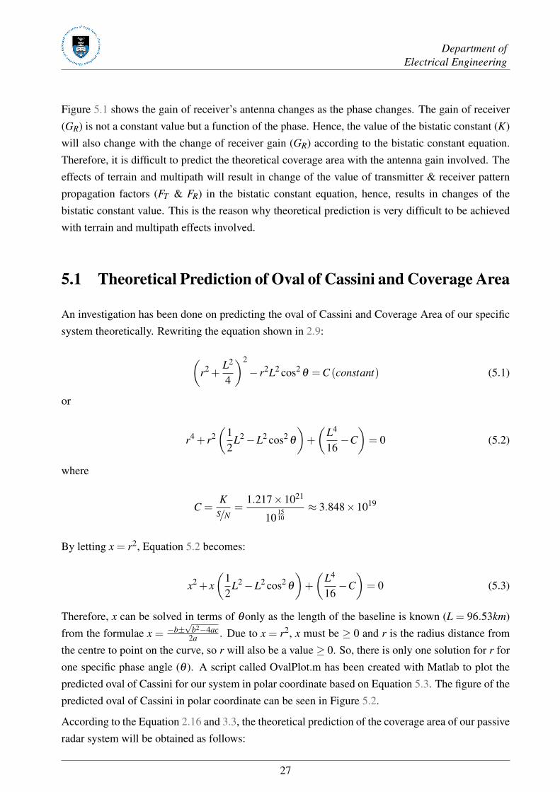
An investigation has been done on predicting the oval of Cassini and Coverage Area of our specificsystem theoretically. Rewriting the equation shown in 2.9:

(r2 +

L2

4

)2

− r2L2 cos2θ = C (constant) (5.1)

or

r4 + r2(

12

L2−L2 cos2θ

)+(

L4

16−C)

= 0 (5.2)

where

C =K

S/N=

1.217×1021

101510

≈ 3.848×1019

By letting x = r2, Equation 5.2 becomes:

x2 + x(

12

L2−L2 cos2θ

)+(

L4

16−C)

= 0 (5.3)

Therefore, x can be solved in terms of θonly as the length of the baseline is known (L = 96.53km)from the formulae x = −b±

√b2−4ac

2a . Due to x = r2, x must be ≥ 0 and r is the radius distance fromthe centre to point on the curve, so r will also be a value ≥ 0. So, there is only one solution for r forone specific phase angle (θ ). A script called OvalPlot.m has been created with Matlab to plot thepredicted oval of Cassini for our system in polar coordinate based on Equation 5.3. The figure of thepredicted oval of Cassini in polar coordinate can be seen in Figure 5.2.

According to the Equation 2.16 and 3.3, the theoretical prediction of the coverage area of our passiveradar system will be obtained as follows:

27


Figure 5.2: Theoretical oval of Cassini plot in polar coordinate for SNR=15dB

A = π×6.204×109

{(1− 1

64

)((9.653×104)4

(6.204×109)2

)−(

316384

)((9.653×104)8

(6.204×109)4

)}≈ 1.8784×104km2

where

L = 9.653×104m and κ =√

KS/N≈ 6.204×109

5.2 Verification of The Theoretical Prediction

In this section, AREPS, MRCPM and a Matlab script called FSArea.m has been used to simulate theSNR coverage map and to integrate the area for desired signal-to-ratio, in order to verify them withthe theoretical prediction that has been done in Chapter 5.1.

5.2.1 Oval of Cassini Verification by using AREPS & MRCPM

As mentioned in Chapter 2.7 and 2.8, the Multistatic Radar Coverage Prediction Method (MRCPM)is a method to plot the SNR coverage maps based on an interpolation of propagation loss data

28


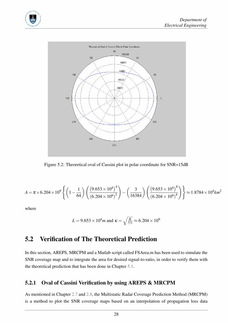
generated by the Advanced Propagation Model (APM) and captured from the Advanced RefractiveEffects Prediction System (AREPS). A SNR coverage map has been created for our system at 5000maltitude in free space by using this method, shown in Figure 5.3.

Figure 5.3: SNR coverage contours at 5000m altitude in free space without antenna gain involved

Figure 5.3 looks very similar to the theoretical SNR coverage map shown in Figure 2.3 in Chapter2.4.3. This is expected, as they both show the SNR coverage contours in free space in a particularbistatic radar system. The colour bar at the right hand side indicates the values of the SNR (in dB) fordifferent ovals of Cassini. The SNR value is getting larger and larger as it gets close to the centre ofthe oval, and at around 25dB, the oval of Cassini breaks into two parts completely. This also verifiesthe simulation from AREPS and MRCPM is consistent with the theoretical equation and prediction.

5.2.2 Coverage Area Verification

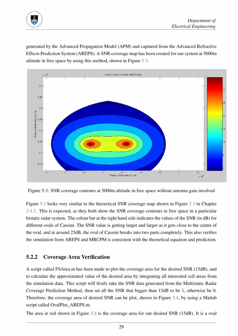
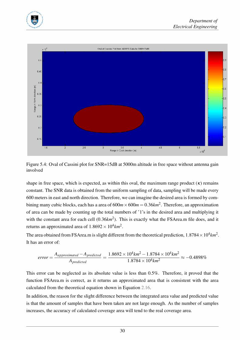
A script called FSArea.m has been made to plot the coverage area for the desired SNR (15dB), andto calculate the approximated value of the desired area by integrating all interested cell areas fromthe simulation data. This script will firstly take the SNR data generated from the Multistatic RadarCoverage Prediction Method, then set all the SNR that bigger than 15dB to be 1, otherwise be 0.Therefore, the coverage area of desired SNR can be plot, shown in Figure 5.4, by using a Matlabscript called OvalPlot_AREPS.m.

The area in red shown in Figure 5.4 is the coverage area for our desired SNR (15dB). It is a oval

29


Figure 5.4: Oval of Cassini plot for SNR=15dB at 5000m altitude in free space without antenna gaininvolved

shape in free space, which is expected, as within this oval, the maximum range product (κ) remainsconstant. The SNR data is obtained from the uniform sampling of data, sampling will be made every600 meters in east and north direction. Therefore, we can imagine the desired area is formed by com-bining many cubic blocks, each has a area of 600m×600m = 0.36km2. Therefore, an approximationof area can be made by counting up the total numbers of ’1’s in the desired area and multiplying itwith the constant area for each cell (0.36km2). This is exactly what the FSArea.m file does, and itreturns an approximated area of 1.8692×104km2.

The area obtained from FSArea.m is slight different from the theoretical prediction, 1.8784×104km2.It has an error of:

error =Aapproximated−Apredicted

Apredicted=

1.8692×104km2−1.8784×104km2

1.8784×104km2 ≈−0.4898%

This error can be neglected as its absolute value is less than 0.5%. Therefore, it proved that thefunction FSArea.m is correct, as it returns an approximated area that is consistent with the areacalculated from the theoretical equation shown in Equation 2.16.

In addition, the reason for the slight difference between the integrated area value and predicted valueis that the amount of samples that have been taken are not large enough. As the number of samplesincreases, the accuracy of calculated coverage area will tend to the real coverage area.

30

Chapter 6

Investigation of the Coverage with AntennaGain, Terrain and Multipath EffectsInvolved

As discussed at the beginning of Chapter 5, it is difficult to predict the coverage with antenna gain,terrain and multipath effects involved theoretically. So, the coverage prediction with these effectswill be carried out by using the AREPS, Multistatic Radar Coverage Prediction Method and theFSArea.m Matlab script in this chapter.

6.1 SNR and Area Coverage with Antenna Gain in free space

The SNR coverage maps that will be shown in this section for the cases that with antenna gaininvolved in free space and not in free space (i.e.: with terrain and multipath effects involved).

Figure 6.1 shows the SNR coverage map with antenna gain in free space. The signal-to-noise-ratiomap looks similar to the antenna gain pattern and with significant high SNR value at the directionof the main-lobe propagation, but low small SNR value at the side-lobe region. This is expected, asthe receiver gain pattern figure(Figure 5.1) shows the antenna gain of the receiver only focus on aparticular phase region (50o−70o).

This type of coverage is actually useful in the application of the aircraft’s detection. This is due tothe fact that each aircraft takes off or lands at the airport will have a set route. Therefore, aircraftswill be active in a particular direction from the airport; by using this coverage method, the passiveradar system can focus on the direction that aircrafts moving toward and away the airport, to improvethe probability of detection and save energy on the receiver’s antenna.

Now, the SNR data with antenna gain involved, which generated from Multistatic Radar CoveragePrediction Method, has been interpolated into OvalPlot_AREPS.m and FSArea.m to plot the cover-

31


Figure 6.1: SNR coverage contours at 5000m altitude in free space with antenna gain involved

age area for SNR=15dB (shown in Figure 6.2) and to calculate its approximated area. The returnedapproximated area is 4.027×104km2.

6.2 SNR and Area Coverage with Antenna Gain and MultipathEffects due to The Flat Ground

Generally, the radar tracks a target aircraft via two paths. One is the direct path from radar to targetand the other path includes a reflection from earth’s surface. Also, the effects of multipath dependon what part of the antenna pattern strikes the surface [8]. Figure 6.3 shows the effects of multipathdue to the flat ground on the SNR coverage map. By comparing the Figures 6.1 and 6.3, notingthat the multipath effects due to the flat ground cause the SNR contours change in shape. The shapebecomes irrational compared to it in free space.

Looking at Figure 6.3 and 6.1, it is evident that the simulated predicted coverage is less comparedto the conventional case which is in free space. The reduction is not unexpected, yet it is importantto note the significant effect that multipath, diffraction, refration and other atmospheric and terraineffects have on the bistatic SNR radar equation and radar detection range.

The SNR data with multipath and terrain effects is interpolated into Matlab scripts called OvalPlot_AREPS.mand FSArea.m. The coverage area for SNR=15dB can be obtained, as shown in Figure 6.4. The ap-proximated area is 4.1121×104km2.

There have been a number of methods demonstrated or proposed for reducing multipath effects, such

32


Figure 6.2: Oval of Cassini plot for SNR=15dB at 5000m altitude in free space with antenna gaininvolved

Figure 6.3: SNR coverage contours at 5000m altitude with antenna gain and multipath effects dueto the flat ground

33


Figure 6.4: Oval of Cassini plot for SNR=15dB at 5000m altitude with antenna gain and multipatheffects due to the flat ground

as Illogical Target Trajectory, Frequency Agility and Double-Null Elevation-Difference Pattern, etc.The details can be seen in [8].

34

Chapter 7

Investigation of Coverage with DifferentAltitude

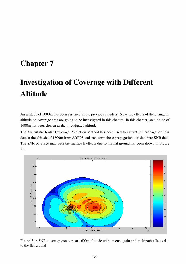
An altitude of 5000m has been assumed in the previous chapters. Now, the effects of the change inaltitude on coverage area are going to be investigated in this chapter. In this chapter, an altitude of1600m has been chosen as the investigated altitude.

The Multistatic Radar Coverage Prediction Method has been used to extract the propagation lossdata at the altitude of 1600m from AREPS and transform these propagation loss data into SNR data.The SNR coverage map with the multipath effects due to the flat ground has been shown in Figure7.1.

Figure 7.1: SNR coverage contours at 1600m altitude with antenna gain and multipath effects dueto the flat ground

35


Figure 7.1 illustrates the simulated prediction coverage for an altitude of 1600m. By comparingthis figure with Figure 6.3 which for an altitude of 5000m, this figure is expected because thereis worse coverage at lower altitudes. At lower altitudes the effects of the multipath and terrain onthe propagation factor have strengthened. Consequently, a close correlation between Figure 7.1 andFigure 6.3 becomes apparent as the AREPS generated propagation loss tends towards free-spacepropagation loss at high altitude.

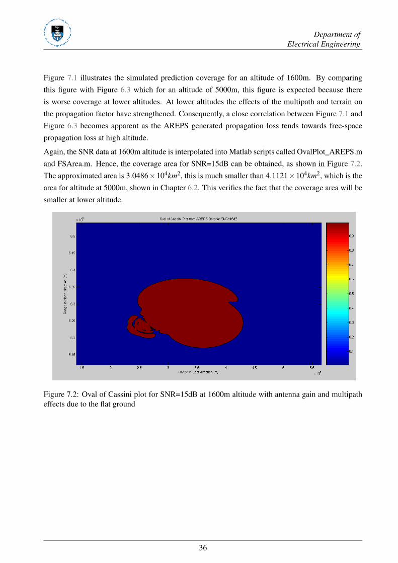
Again, the SNR data at 1600m altitude is interpolated into Matlab scripts called OvalPlot_AREPS.mand FSArea.m. Hence, the coverage area for SNR=15dB can be obtained, as shown in Figure 7.2.The approximated area is 3.0486×104km2, this is much smaller than 4.1121×104km2, which is thearea for altitude at 5000m, shown in Chapter 6.2. This verifies the fact that the coverage area will besmaller at lower altitude.

Figure 7.2: Oval of Cassini plot for SNR=15dB at 1600m altitude with antenna gain and multipatheffects due to the flat ground

36

Chapter 8

Investigation of Coverage for An OneTransmitter & Two Receivers Passive RadarSystem

The coverage for one transmitter and one receiver passive radar system has been analysed in Chapter3 to Chapter 7. A two transmitters and one receiver passive radar system is going to be investigatedin this chapter.

8.1 Problem Discussion

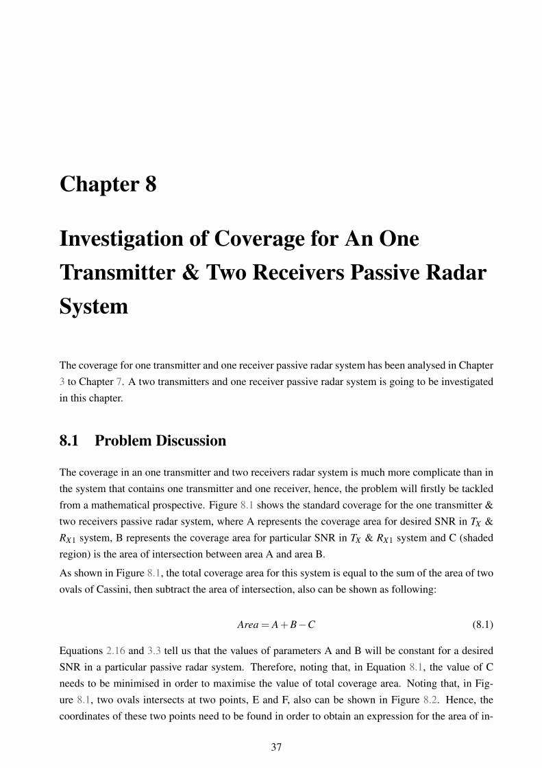
The coverage in an one transmitter and two receivers radar system is much more complicate than inthe system that contains one transmitter and one receiver, hence, the problem will firstly be tackledfrom a mathematical prospective. Figure 8.1 shows the standard coverage for the one transmitter &two receivers passive radar system, where A represents the coverage area for desired SNR in TX &RX1 system, B represents the coverage area for particular SNR in TX & RX1 system and C (shadedregion) is the area of intersection between area A and area B.

As shown in Figure 8.1, the total coverage area for this system is equal to the sum of the area of twoovals of Cassini, then subtract the area of intersection, also can be shown as following:

Area = A+B−C (8.1)

Equations 2.16 and 3.3 tell us that the values of parameters A and B will be constant for a desiredSNR in a particular passive radar system. Therefore, noting that, in Equation 8.1, the value of Cneeds to be minimised in order to maximise the value of total coverage area. Noting that, in Fig-ure 8.1, two ovals intersects at two points, E and F, also can be shown in Figure 8.2. Hence, thecoordinates of these two points need to be found in order to obtain an expression for the area of in-

37


Figure 8.1: Diagram for a standard one transmitter & two receivers passive radar system

tersection. Noting the fact that, both ovals can be expressed in polar coordinates (r,θ) with its originlying on the mid-point of each baseline which is shown in Equation 2.9. For a better investigation, itwill be easier if both origin of axes can be shifted to the point where the transmitter located, as thetransmitter is located within the area of intersection and it is the essential link between two ovals.An investigation has been carried out by mathematical calculation to minimise the intersection areaof two ovals, as shown in the following chapters.

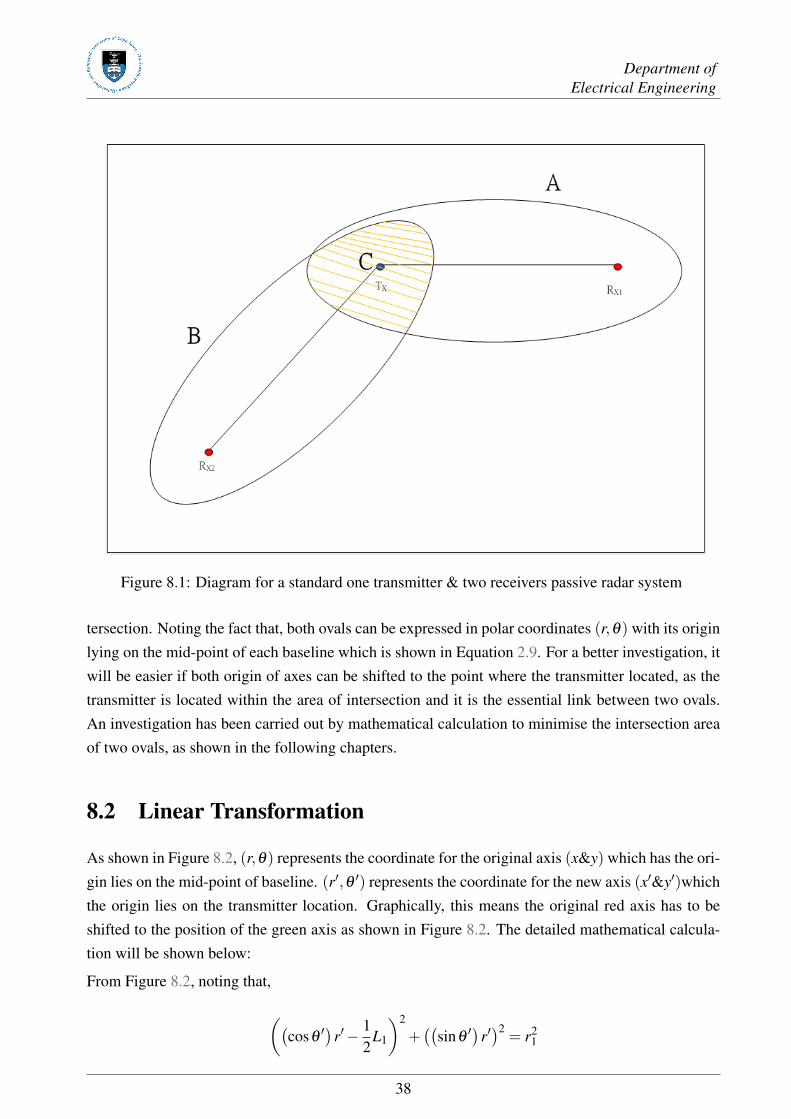
8.2 Linear Transformation

As shown in Figure 8.2, (r,θ) represents the coordinate for the original axis (x&y) which has the ori-gin lies on the mid-point of baseline. (r′,θ ′) represents the coordinate for the new axis (x′&y′)whichthe origin lies on the transmitter location. Graphically, this means the original red axis has to beshifted to the position of the green axis as shown in Figure 8.2. The detailed mathematical calcula-tion will be shown below:

From Figure 8.2, noting that,

((cosθ

′)r′− 12

L1

)2

+((

sinθ′)r′)2 = r2

1

38


Figure 8.2: Diagram for the illustration of linear transformation

((cosθ)r +

12

L1

)2

+((sinθ)r)2 =(r′)2

and

(sinθ1)r1 =(sinθ

′)r′ (8.2)

Solving the above two equations, r1and θ1 can be expressed in the terms of r′ and θ ′.

r1 = f(r′,θ ′

)=

√r′2− r′L1 cosθ ′+

14

L21

θ1 = f(r′,θ ′

)= sin−1

r′ sinθ ′√r′2− r′L1 cosθ ′+ 1

4L21

In addition, r′ and θ ′ in terms of r1 and θ1can also be obtained.

r′ = f (r1,θ1) =

√r2

1 + r1L1 cosθ1 +14

L21 (8.3)

39


θ′ = f (r1,θ1) = sin−1

r1 sinθ1√r2

1 + r1L1 cosθ1 + 14L2

1

(8.4)

A Matlab script called transformation.m has been created to check and ensure the equations that havebeen obtain shown above are correct. The description of this script will be shown in the AppendixA.

8.3 Linear Transformation with Rotation

Figure 8.3: Diagram for the illustration of linear transformation with rotation

Figure 8.3 shows the oval of Cassini diagram for the TX and RX2 system. α is the angle betweenbaselines L1 and L2. Axis (x2&y2)is the original axis for this oval, and axis (x′&y′) is the newaxis which is the same axis as shown in Figure 8.2. The anti-clockwise direction is assumed to bethe positive direction, hence, the coordinate of point B with respect to the axis (x′&y′)is (r”,θ”).Noting that, β = θ”+α−2π . Applying the same method that was used in previous paragraph, thefollowing expressions can be yielded.

r2and θ2 can be expressed in the terms of r” and θ”:

40


r2 = f (r”,θ”) =

√r”2− r”L2 cos(θ”+α−2π)+

14

L22

θ2 = f (r”,θ”) = sin−1

r”sin(θ”+α−2π)√r”2− r”L2 cos(θ”+α−2π)+ 1

4L22

In addition, r” and θ” in terms of r2 and θ2can also be obtained.

r” = f (r2,θ2) =

√r2

2 + r2L2 cosθ2 +14

L22 (8.5)

θ” = 2π +β −α = 2π + sin−1

r2 sinθ2√r2

2 + r2L2 cosθ2 + 14L2

2

−α (8.6)

Also, a Matlab script called Rotation.m has been created to check and ensure the equations that havebeen obtain shown above are correct. The description of this script will be shown in the AppendixA.

As shown in Figure 8.3, intersecting points of two oval, point E and F, their coordinates with respectto the oval contains Rx1will be the same as the coordinates with respect to the oval contains Rx2whichall corresponding to the axis located on the transmitter position. This simply means that at point Eand F, they both has r′ = r”and θ ′ = θ”. Therefore, intersecting points, E and F, can be solved byequating Equation 8.3 and 8.5, and Equation 8.4 and 8.6. The following equations can be obtained:

√r2

1 + r1L1 cosθ1 +14

L21 =

√r2

2 + r2L2 cosθ2 +14

L22

and

sin−1

r1 sinθ1√r2

1 + r1L1 cosθ1 + 14L2

1

= 2π + sin−1

r2 sinθ2√r2

2 + r2L2 cosθ2 + 14L2

2

−α

However, it is very difficult to solve the above equations mathematically due to their non-linearity.The area of intersection will, therefore, be simulated with Matlab based on the expressions shown inabove.

41


8.4 Simulation of Area of Intersection for Two Ovals with Mat-lab

Firstly, for avoiding complexity, the following assumption has been made in this one transmitter andtwo receivers system:

L1 = L2 = L

Recording the polar coordinate Equation 5.2 shown in Chapter 5.1, the radius from the origin to thepoint on the curve (r) can be expressed in terms of the angle (θ ) in a oval of Cassini. The expressionis shown as following:

r =

√√√√√−(12L2−L2 cos2 θ

)+√(1

2L2−L2 cos2 θ)2−4

(L4

16 −K

S/N

)2

(8.7)

By substituting Equation 8.7 into Equation 8.3 and 8.4 separately, the r′and θ ′in terms of θ only,can be obtained. r”and θ” in terms of θ only can also be obtained by substituting Equation 8.7 intoEquation 8.5 and 8.6 separately. θ has been set to be a matrix contains phase from 0 to 2πwith stepof 1 degree. Therefore, r′ and θ ′, r”and θ”, can be plotted in polar coordinate with the transmitterlocated at the origin. α is needed to be specified in order to simulate and plot the area of intersectionfor two ovals. So, α will be set to be 120 degrees (2

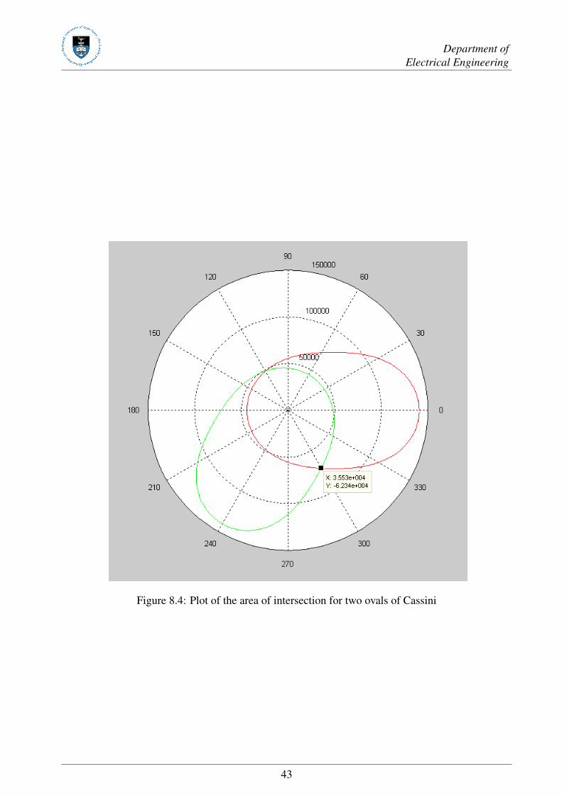
3π in radian). Hence, Figure 8.4 has been createdby using Matlab script called OvalPlot_transfo_coordinate.m.

The position of the point of intersection for two ovals can be measured directly from the simulatedplot in Matlab. After obtaining position of these two intersecting points, the two curves that enclosethe area of intersection have been given. The value of the area of intersection can then be found byintegrating each cell area within the intersected area in the Cartesian grid. However, these tasks havenot been carried out in detail due to the time constrain of this project.

42


Figure 8.4: Plot of the area of intersection for two ovals of Cassini

43

Chapter 9

Conclusions and Future Work

This project report focuses on the optimisation of the location of receiver site by investigating thecoverage for a passive radar system. A method of maximising the coverage for an one transmitter andone receiver case of passive radar system has been obtained during the investigation. A suggestionon achieving maximum coverage for an one transmitter and two receivers case of passive radar hasalso been provided.

The establishment of a firm literary base was believed important. Thus to this end, a great deal ofliterature was studied and reviewed, this review of literature is ultimately presented in Chapter 2 ofthis project report.

The actual analytical work done in this project report began by setting a criterion for the investigatedpassive radar system. Thereafter, the relationship between SNR, baseline and coverage area hasbeen investigate. The fact that, for a specific SNR, coverage area in a given one transmitter and onereceiver passive radar system only depends on the length of baseline (L). The longer the distancebetween the transmitter and receiver, the less coverage area will be.

A comparison between the theoretical prediction and the simulated prediction without antenna gaininvolved in free space has been made. The effects of the antenna gain, multipath, terrain and changein altitude on the coverage area have also been discussed. This is followed by investigating the cover-age area in an one transmitter and two receivers passive radar system mathematically. A suggestionhas been provided to maximise the coverage area for this case.

In terms of future work, much additional analytical work can be done to further the investigationsbegun in this project report. In particular, the investigations done in Chapter 8 can be furthered byintegrating the area of two enclosed curves from two ovals, hence, to minimise the area of inter-section in order to maximise the total coverage area. Due to the limitation of the equipment, allthe work done in this project report was in pure theoretical and simulated nature, therefore, all theinvestigations and analyses carried out here could be verified by practical experiment. In the future,the final goal of this topic is the optimum receiver site can be found automatically in any passiveradar system by doing simulation with the realistic data involved.

44

Appendix A

Matlab Code Description

The Matlab scripts written for this thesis can be found on the CD provided. This appendix lists allthe m.files used in this project and gives brief description for each m.file.

Area_vs_Baseline_Plot.m

This stand alone Matlab script will plot the relationship between the coverage and baseline based onthe theoretical equation of passive radar area coverage.

FSArea.m

This function will take the SNR data that is generated from AREPS and Multistatic Radar CoveragePrediction Method, then it will count the total number of the desired SNR contained in the SNR data.Therefore, approximated area for the desired SNR can be obtain by multiplying this total numberwith the area of each cell in the Cartesian grid.

gain_vs_phase_plot.m

This script will plot the antenna gain pattern of the receiver in our practical radar system.

OvalPlot.m

The theoretical oval of Cassini plot for a desired SNR can be obtained by using this Matlab script.

OvalPlot_AREPS.m

This function will take the SNR data produced from the MRCPM, plot the SNR coverage map forthe particular passive radar system firstly; Secondly, it will make all the SNR values that bigger than15dB to be 1 and 0 otherwise. So, a desired SNR coverage area will also be plotted in this Matlabfunction.

45


OvalPlot_transfo_coordinate.m

This Matlab script is used to simulate and plot the area of intersection of two ovals based on theequations shown in Chapter 8. Therefore, the coordinates of the points of intersection for two ovalscan be obtained. In addition, the plot is plotted with the transmitter sits at the origin of the plot.

Rotation.m

This script is used to verify the equations that obtained from the mathematical prospective shown inChapter 8. As the fact that the position of the transmitter is given, this script will take a point on thecurve of the oval, (r,θ), and use the chosen point to obtain the distance and angle from the transmit-ter to the point, r′ and θ ′, with irrespectively. By substituting r′ and θ ′ value into the equation for r

and θ which are in terms of r′ and θ ′ in order to obtain the theoretical r and θ value. By comparingthe theoretical r and θwith the coordinate of the chosen point. If they are identical, it proves that themathematical prediction is correct.

transformation.m

This script uses the same method shown in Rotation.m to verify the expression for the linear trans-formation with rotation involved.

46

Appendix B

CD

This project report comes with a CD containing:

• All Matlab scripts discussed in this project report.

• A PDF version of this project report.

47

Bibliography

[1] User’s Manual (UM) for Advanced Refractive Effects Prediction System. Atmospheric Prop-agation Branch, Space and Naval Warfare System Centre, San Diego, CA, 3.6 edition edition,December 2006.

[2] Atmospheric Propagation Branch. Software programs - introduction of areps. October 2008.URL http://areps.spawar.navy.mil/.

[3] James and James. Mathematics dictionary. Van Nostrand, New York, 1949.

[4] Gunther Lange. Multistatic radar coverage prediction method. August 2008.

[5] R.J. Lefevre. Bistatic radar: New application for an old technique. In WESCON Conf. Record,

San Francisco, pages 1–20, 1979.

[6] Christopher L. Zoeller; Dr Mervin C. Budge; Jr. Michael J. Moody. Passive coherent locationradar demonstration. 2002.

[7] Hovanessian SA. Radar System Design and Analysis. Artech House, January 1984.

[8] Merrill I. Skolnik. Introduction to Radar Systems 3rd ed. McGraw-Hill, 2001.

[9] Wikipedia. the free encyclopedia - bistatic radar. October 2008. URL http://en.wikipedia.

org/wiki/Bistatic_radar.

[10] Wikipedia. the free encyclopedia - passive radar. October 2008. URL http://en.

wikipedia.org/wiki/Passive_radar.

[11] Nicholas J. Willis. Bistatic Radar. SciTech Publishing, Inc., 2005.

48

http://areps.spawar.navy.mil/

http://en.wikipedia.org/wiki/Bistatic_radar

http://en.wikipedia.org/wiki/Bistatic_radar

http://en.wikipedia.org/wiki/Passive_radar

http://en.wikipedia.org/wiki/Passive_radar

Receiver Site Optimisation for Passive Coherent...

Documents

Transcript of Receiver Site Optimisation for Passive Coherent...